ppl electric utilities corporation exhibit … as used in accounting, is a method of distributing...

PPL ELECTRIC UTILITIES CORPORATION

Exhibit JJS 2

Depreciation Study Related to Electric Plant At December 31, 2012

Witness: John J. Spanos

Docket No. R-2012-2290597


ALLENTOWN, PENNSYLVANIA

DEPRECIATION STUDY

CALCULATED ANNUAL DEPRECIATION ACCRUALS RELATED TO ELECTRIC PLANT AT

DECEMBER 31, 2012

EXHIBIT JJS 2

PPL ELECTRIC UTILITIES CORPORATIONAllentown, Pennsylvania

DEPRECIATION STUDY

CALCULATED ANNUAL DEPRECIATION ACCRUALSRELATED TO ELECTRIC PLANT

AT DECEMBER 31, 2012

EXHIBIT JJS 2

GANNETT FLEMING, INC. - VALUATION AND RATE DIVISION

Harrisburg, Pennsylvania

iii

C O N T E N T S

PART I. EXECUTIVE SUMMARY

Scope . . . . . . . . . . . . . . . . . . . . . . . . . . . . . . . . . . . . . . . . . . . . . . . . . . . . . . . I-2Basis of Study . . . . . . . . . . . . . . . . . . . . . . . . . . . . . . . . . . . . . . . . . . . . . . . . . I-2

Depreciation and Amortization . . . . . . . . . . . . . . . . . . . . . . . . . . . . . . . I-2Service Life Estimates . . . . . . . . . . . . . . . . . . . . . . . . . . . . . . . . . . . . . I-3

Amortization of Net Salvage . . . . . . . . . . . . . . . . . . . . . . . . . . . . . . . . . . . . . . I-4

PART II. METHODS USED IN THE DETERMINATIONOF ANNUAL AND ACCRUED DEPRECIATION

Depreciation . . . . . . . . . . . . . . . . . . . . . . . . . . . . . . . . . . . . . . . . . . . . . . . . . . II-2Life Analysis . . . . . . . . . . . . . . . . . . . . . . . . . . . . . . . . . . . . . . . . . . . . . . . . . . II-3

Average Service Life . . . . . . . . . . . . . . . . . . . . . . . . . . . . . . . . . . . . . . II-3Survivor Curves . . . . . . . . . . . . . . . . . . . . . . . . . . . . . . . . . . . . . . . . . . II-3Iowa Type Curves . . . . . . . . . . . . . . . . . . . . . . . . . . . . . . . . . . . . . . . . II-4Retirement Rate Method of Analysis . . . . . . . . . . . . . . . . . . . . . . . . . . II-11

Schedules of Annual Transactions in Plant Records . . . . . . . . . II-12Schedule of Plant Exposed to Retirement . . . . . . . . . . . . . . . . . II-15Original Life Table . . . . . . . . . . . . . . . . . . . . . . . . . . . . . . . . . . . II-17Smoothing the Original Survivor Curve . . . . . . . . . . . . . . . . . . . II-19

Judgment . . . . . . . . . . . . . . . . . . . . . . . . . . . . . . . . . . . . . . . . . . . . . . . II-24Calculation of Annual and Accrued Depreciation . . . . . . . . . . . . . . . . . . . . . . II-26

Group Depreciation Procedures . . . . . . . . . . . . . . . . . . . . . . . . . . . . . . II-26Remaining Life Annual Accruals . . . . . . . . . . . . . . . . . . . . . . . . . . . . . II-27Average Service Life Procedure . . . . . . . . . . . . . . . . . . . . . . . . . . . . . II-27

Calculation of Annual and Accrued Amortization . . . . . . . . . . . . . . . . . . . . . . II-28

PART III. RESULTS OF STUDY

Qualification of Results . . . . . . . . . . . . . . . . . . . . . . . . . . . . . . . . . . . . . . . . . . III-2Description of Statistical Support . . . . . . . . . . . . . . . . . . . . . . . . . . . . . . . . . . III-2Description of Depreciation Tabulations . . . . . . . . . . . . . . . . . . . . . . . . . . . . . III-3Table 1. Estimated Survivor Curves, Original Cost, Book Reserve and

Calculated Annual Depreciation Accruals Related to Utility Plant at December 31, 2012 . . . . . . . . . . . . . . . . . . . . . . . . . . . . . . . . . . . . . . III-4Table 2. Bringforward of the Book Reserve from December 31, 2011

to December 31, 2012 . . . . . . . . . . . . . . . . . . . . . . . . . . . . . . . . . . . . . . III-6Table 3. Summary of Net Salvage by Function and Amortization

for the Period, 2008-2012 . . . . . . . . . . . . . . . . . . . . . . . . . . . . . . . . . . . . III-8Service Life Statistics . . . . . . . . . . . . . . . . . . . . . . . . . . . . . . . . . . . . . . . . . . . III-9Detailed Depreciation Calculations . . . . . . . . . . . . . . . . . . . . . . . . . . . . . . . . . III-146

I-2


DEPRECIATION STUDYCALCULATED ANNUAL DEPRECIATION ACCRUALS

RELATED TO ELECTRIC PLANT AT DECEMBER 31, 2012


SCOPE

This report presents the results of the depreciation study as applied to electric plant

in service as of December 31, 2012. The Valuation and Rate Division of Gannett Fleming,

Inc., prepared this report on behalf of PPL Electric Utilities Corporation. It relates to the

concepts, methods and basic judgments which underlie recommended annual depreciation

accrual rates related to current electric plant in service.

The annual depreciation accrual rates and amounts presented herein are based on

an updated service life study incorporating data through 2007 prepared pursuant to the

rules of 52 Pa. Code, Chapter 73.6. The prior service life study was based on data through

2002.

BASIS OF STUDY

Depreciation and Amortization. For most plant accounts, depreciation accruals and

accrued depreciation were calculated using the straight line method, the remaining life

basis, and the average service life procedure for all vintages.

The depreciation calculations were based on the attained ages and estimated

service life characteristics for each depreciable group of electric plant. For certain general

plant accounts, the amortization amounts, annual and accrued, were based on the age of

the vintage and the selected amortization period.

Survivor curves were used to reflect the expected dispersion of retirements, thus

providing a consistent method of estimating service lives and depreciation for mass

I-3

property. Iowa type curves were used to depict the estimated survivor curves. For life

span groups, the estimate of life characteristics is consistent, because the calculated lives

of the units within a group are obtained by employing a single probable retirement date for

the entire group.

Service Life Estimates. The method of estimating service life consisted of compiling

the service life history of the plant accounts, subaccounts or depreciable groups, reducing

this history to trends through the use of acceptable actuarial techniques, and forecasting

the trend of survivors for each depreciable group on the basis of interpretations of past

trends and consideration of Company plans for the future. The combination of the historical

trend and the estimated future trend yielded a complete pattern of life characteristics from

which the average service life was derived.

The service life estimates incorporated historical data compiled through 2007 from

the property records of the Company. Such data included plant additions, retirements,

transfers and other activity. Generally, retirement data for the years 1937 through 2007

were used in the actuarial life table computations which were the primary statistical support

of the service life estimates.

A general understanding of the function of the plant and information with respect to

the reasons for past retirements and the expected future causes of retirement was obtained

through field trips conducted during the service life study. Discussions with operating and

management personnel also provided information regarding plans for the future which was

incorporated in the interpretation and extrapolation of the statistical analyses.

Amortization of Net Salvage. Inasmuch as this report relates primarily to

Pennsylvania rate regulation practices, under which experienced costs of negative net

I-4

salvage are amortized after their occurrence, no adjustments for expected salvage were

made to either the annual depreciation accrual or the calculated accrued depreciation for

the individual accounts. The annual provision for recovering negative net salvage is based

on the amortization of experienced net salvage over a five-year period, as established in

the Commission order at Docket No. R-00943271.

II-2


DEPRECIATION

Depreciation, as defined in the Uniform System of Accounts, is the loss in service

value not restored by current maintenance, incurred in connection with the consumption

or prospective retirement of electric plant in the course of service from causes which are

known to be in current operation and against which the utility is not protected by insurance.

Among the causes to be given consideration are wear and tear, decay, action of the

elements, inadequacy, obsolescence, changes in the art, changes in demand, and

requirements of public authorities.

Depreciation, as used in accounting, is a method of distributing fixed capital costs

over a period of time by allocating annual amounts to expense. Each annual amount of

such depreciation expense is part of that year's total cost of providing utility service.

Normally the period of time over which the fixed capital cost is allocated to the cost of

service is equal to the period of time over which an item renders service, that is, the item's

service life. The most prevalent method of allocation is to distribute an equal amount of

cost to each year of service life. This method is known as the straight line method of

depreciation.

The calculation of annual and accrued depreciation based on the straight line

method requires the estimation of survivor curves and the selection of group depreciation

procedures. These subjects are discussed in the sections which follow.

II-3

LIFE ANALYSIS

Average Service Life

The use of an average service life for a property group implies that the various units

in the group have different lives. Thus, the average life may be obtained by determining

the separate lives of each of the units, or by constructing a survivor curve by plotting the

number of units which survive at successive ages. The use of survivor curves, which

reflect experienced and expected dispersion of service lives, is a systematic and rational

means of estimating average service lives to be used to calculate depreciation for utility

property. A discussion of the general concept of survivor curves and the Iowa type survivor

curves is presented.

Survivor Curves

The survivor curve graphically depicts the amount of property existing at each age

throughout the life of an original group. From the survivor curve, the average life of the

group, the remaining life expectancy, the probable life and the frequency curve can be

calculated. In Figure 1, a typical smooth survivor curve and the derived curves are

illustrated. The average life is obtained by calculating the area under the survivor curve,

from age zero to the maximum age, and dividing this area by the ordinate at age zero. The

remaining life expectancy at any age can be calculated by obtaining the area under the

curve, from the observation age to the maximum age, and dividing this area by the percent

surviving at the observation age. For example, in Figure 1 the remaining life at age 30

years is equal to the crosshatched area under the survivor curve divided by 29.5 percent

surviving at age 30. The probable life at any age is developed by adding the age and

II-4

remaining life. If the probable life of the property is calculated for each year of age, the

probable life curve shown in the chart can be developed. The frequency curve presents

the number of units retired in each age interval and is derived by obtaining the differences

between the amount of property surviving at the beginning and at the end of each interval.

Iowa Type Curves. The range of survivor characteristics usually experienced by

utility and industrial properties is encompassed by a system of generalized survivor curves

known as the Iowa type curves. There are four families in the Iowa system, labeled in

accordance with the location of the modes of the retirements in relationship to the average

life and the relative height of the modes. The left moded curves, presented in Figure 2, are

those in which the greatest frequency of retirement occurs to the left of, or prior to, average

service life. The symmetrical moded curves, presented in Figure 3, are those in which the

greatest frequency of retirement occurs at average service life. The right moded curves,

presented in Figure 4, are those in which the greatest frequency occurs to the right of, or

after, average service life. The origin moded curves, presented in Figure 5, are those in

which the greatest frequency of retirement occurs at the origin, or immediately after age

zero. The letter designation of each family of curves (L, S, R or O) represents the location

of the mode of the associated frequency curve with respect to the average service life. The

numerical subscripts represent the relative heights of the modes of the frequency curves

within each family.

The Iowa curves were developed at the Iowa State College Engineering Experiment

Station through an extensive process of observation and classification of the ages at which

industrial property had been retired. A report of the study which resulted in the classifica-

tion of property survivor characteristics into 18 type curves, which constitute three of the

1Winfrey, Robley. Statistical Analyses of Industrial Property Retirements. IowaState College, Engineering Experiment Station, Bulletin 125. 1935.

2Marston, Anson, Robley Winfrey and Jean C. Hempstead. Engineering Valuationand Depreciation, 2nd Edition. New York, McGraw-Hill Book Company. 1953.

3Couch, Frank V. B., Jr. "Classification of Type O Retirement Characteristics ofIndustrial Property." Unpublished M.S. thesis (Engineering Valuation). Library, Iowa StateCollege, Ames, Iowa. 1957.

II-10

four families, was published in 1935 in the form of the Experiment Station's Bulletin 1251.

These type curves have also been presented in subsequent Experiment Station bulletins

and in the text, "Engineering Valuation and Depreciation2." In 1957, Frank V. B. Couch, Jr.,

an Iowa State College graduate student, submitted a thesis3 presenting his development

of the fourth family consisting of the four O type survivor curves.

Survivor curves for groups in which all property is expected to be retired

concurrently, such as power plants, are obtained by truncating smooth survivor curves at

an age before zero percent surviving is reached. Such groups to which truncated survivor

curves are applicable are designated as life span groups. In life span groups of one or

more vintages, future retirements of all property included in the group are anticipated to

occur at a specific date or over a restricted range of future dates which are represented by

an estimated probable retirement date. Survivor curves for life span groups can be

developed using both available historical experience and known or forecasted retirement

dates. The life span of both the original installation and a subsequent addition is the

number of years which elapse between its installation and the final retirement of the group.

During the life of the group as a whole, interim retirements normally occur between age

zero and the maximum age to produce a survivor pattern which is referred to as an "interim

survivor curve".

4Winfrey, Robley, Supra Note 1.

5Marston, Anson, Robley Winfrey, and Jean C. Hempstead, Supra Note 2.

6A Report of the Engineering Subcommittee of the Depreciation AccountingCommittee, Edison Electric Institute. Publication No. 51-23. Published 1952.

II-11

Retirement Rate Method of Analysis

The retirement rate method is an actuarial method of deriving survivor curves using

the average rates at which property of each age group is retired. The method relates to

property groups for which aged accounting experience is available or for which aged

accounting experience is developed by statistically aging unaged amounts and is the

method used to develop the original stub survivor curves in this study. The method (also

known as the annual rate method) is illustrated through the use of an example in the

following text, and is also explained in several publications, including "Statistical Analyses

of Industrial Property Retirements,"4 "Engineering Valuation and Depreciation"5 and

"Methods of Estimating Utility Plant Life".6

The average rate of retirement used in the calculation of the percent surviving for

the survivor curve (life table) requires two sets of data: first, the property retired during a

period of observation, identified by the property's age at retirement; and second, the

property exposed to retirement at the beginnings of the age intervals during the same

period. The period of observation is referred to as the experience band, and the band of

years which represent the installation dates of the property exposed to retirement during

the experience band is referred to as the placement band. An example of the calculations

used in the development of a life table based on the age at retirement in years follows.

II-12

The example includes schedules of annual aged property transactions, a schedule of

plant exposed to retirement, a life table and illustrations of smoothing the stub survivor

curve.

Schedules of Annual Transactions in Plant Records. The property group used to

illustrate the retirement rate method is observed for the experience band 2002-2011 during

which there were placements during the years 1997-2011. In order to illustrate the

summation of the aged data by age interval, the data were compiled in the manner

presented in Schedules 1 and 2 on pages II-13 and II-14. In Schedule 1, the year of

installation (year placed) and the year of retirement are shown. The age interval during

which a retirement occurred is determined from this information. In the example which

allows, $10,000 of the dollars invested in 1997 were retired in 2002. The $10,000

retirement occurred during the age interval between 4½ and 5½ years on the basis that

approximately one-half of the amount of property was installed prior to and subsequent to

July 1 of each year. That is, on the average, property installed during a year is placed in

service at the midpoint of the year for the purpose of the analysis. All retirements also are

stated as occurring at the midpoint of a one-year age interval of time, except the first age

interval which encompasses only one-half year.

The total retirements occurring in each age interval in a band are determined by

summing the amounts for each transaction year-installation year combination for that age

interval. For example, the total of $143,000 retired for age interval 4½-5½ is the sum of the

retirements entered on Schedule 1 immediately above the stairstep line drawn on the table

beginning with the 2002 retirements of 1997 installations and ending with the 2011

retirements of the 2006 installations. Thus, the total amount of 143 for age interval 4½-5½

equals the sum of:

10 + 12 + 13 + 11 + 13 + 13 + 15 + 17 + 19 + 20.

TABLE 1. RETIREMENTS FOR EACH YEAR 2002-2011SUMMARIZED BY AGE INTERVAL

Experience Band 2002-2011 Placement Band 1997-2011 Retirements, Thousands of Dollars

YearPlaced

During Year Total DuringAge Interval

Age Interval 2002 2003 2004 2005 2006 2007 2008 2009 2010 2011

(1) (2) (3) (4) (5) (6) (7) (8) (9) (10) (11) (12) (13)

1997 10 11 12 13 14 16 23 24 25 26 26 13½-14½ 1998 11 12 13 15 16 18 20 21 22 19 44 12½-13½ 1999 11 12 13 14 16 17 19 21 22 18 64 11½-12½ 2000 8 9 10 11 11 13 14 15 16 17 83 10½-11½ 2001 9 10 11 12 13 14 16 17 19 20 93 9½-10½ 2002 4 9 10 11 12 13 14 15 16 20 105 8½-9½ 2003 5 11 12 13 14 15 16 18 20 113 7½-8½ 2004 6 12 13 15 16 17 19 19 124 6½-7½ 2005 6 13 15 16 17 19 19 131 5½-6½ 2006 7 14 16 17 19 20 143 4½-5½ 2007 8 18 20 22 23 146 3½-4½ 2008 9 20 22 25 150 2½-3½ 2009 11 23 25 151 1½-2½ 2010 11 24 153 ½-1½ 2011 13 80 0-½

Total 53 68 86 106 128 157 196 231 273 308 1,606

II-13

TABLE 2. OTHER TRANSACTIONS FOR EACH YEAR 2002-2011SUMMARIZED BY AGE INTERVAL

Experience Band 2002-2011 Placement Band 1997-2011

Acquisitions, Transfers and Sales, Thousands of Dollars Year During Year Total During Age

Placed(1)

2002(2)

2003(3)

2004 (4)

2005(5)

2006(6)

2007(7)

2008(8)

2009(9)

2010(10)

2011(11)

Age Interval(12)

Interval (13)

1997 - - - - - - 60a - - - - 13½-14½1998 - - - - - - - - - - - 12½-13½1999 - - - - - - - - - - - 11½-12½2000 - - - - - - - (5)b - - 60 10½-11½2001 - - - - - - - 6 a - - - 9½-10½2002 - - - - - - - - - (5) 8½-9½2003 - - - - - - - - - 6 7½-8½2004 - - - - - - - - - 6½-7½2005 - - - - (12)b - - - 5½-6½2006 - - - - 22a - - 4½-5½2007 - - (19)b - - 10 3½-4½2008 - - - - - 2½-3½2009 - - (102)c (121) 1½-2½2010 - - - ½-1½2011 - 0-½

Total - - - - - - 60 (30) 22 (102) ( 50)

a Transfer Affecting Exposures at Beginning of Yearb Transfer Affecting Exposures at End of Yearc Sale with Continued UseParentheses denote Credit amount.

II-14

II-15

In Schedule 2, other transactions which affect the group are recorded in a similar

manner. The entries illustrated include transfers and sales. The entries which are credits

to the plant account are shown in parentheses. The items recorded on this schedule are

not totaled with the retirements but are used in developing the exposures at the beginning

of each age interval.

Schedule of Plant Exposed to Retirement. The development of the amount of plant

exposed to retirement at the beginning of each age interval is illustrated in Schedule 3 on

page II-16.

The surviving plant at the beginning of each year from 2002 through 2011 is

recorded by year in the portion of the table headed "Annual Survivors at the Beginning of

the Year". The last amount entered in each column is the amount of new plant added to

the group during the year. The amounts entered in Schedule 3 for each successive year

following the beginning balance or addition are obtained by adding or subtracting the net

entries shown on Schedules 1 and 2. For the purpose of determining the plant exposed

to retirement, transfers-in are considered as being exposed to retirement in this group at

the beginning of the year in which they occurred, and the sales and transfers-out are

considered to be removed from the plant exposed to retirement at the beginning of the

following year. Thus, the amounts of plant shown at the beginning of each year are the

amounts of plant from each placement year considered to be exposed to retirement at

the beginning of each successive transaction year. For example, the exposures for the

installation year 2007 are calculated in the following manner:

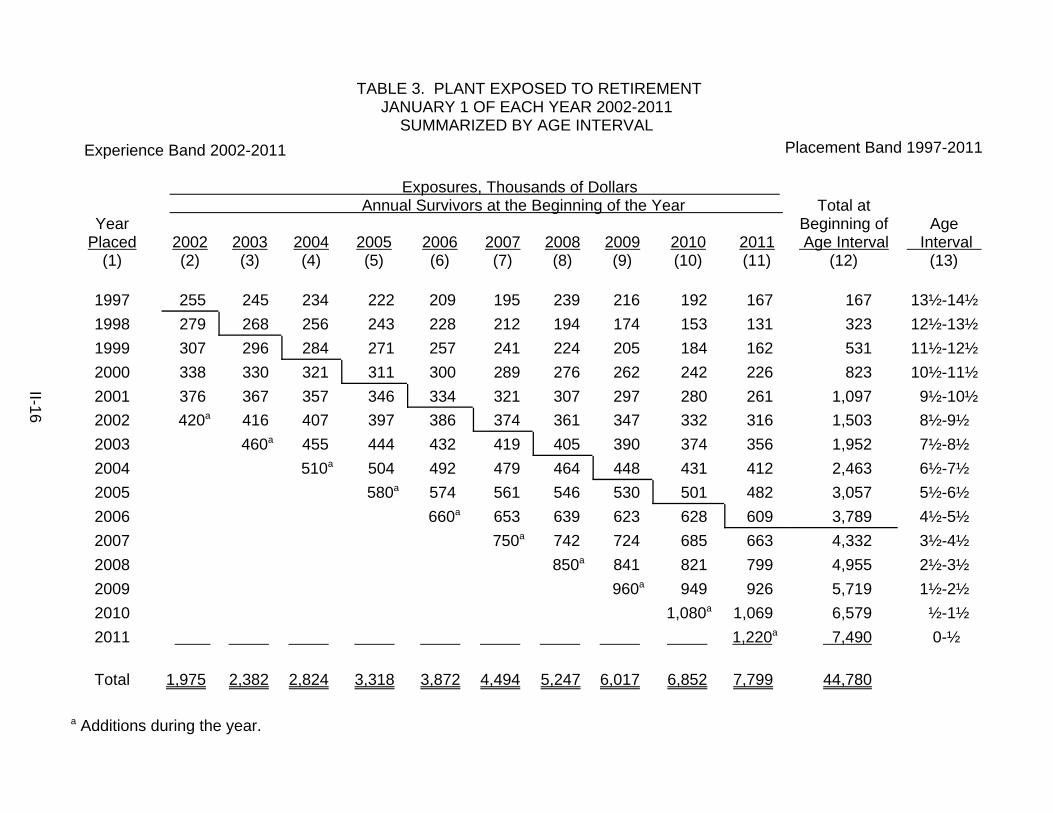
TABLE 3. PLANT EXPOSED TO RETIREMENTJANUARY 1 OF EACH YEAR 2002-2011

SUMMARIZED BY AGE INTERVAL Experience Band 2002-2011 Placement Band 1997-2011

Exposures, Thousands of Dollars Annual Survivors at the Beginning of the Year Total at

YearPlaced

Beginning of Age Interval

Age Interval 2002 2003 2004 2005 2006 2007 2008 2009 2010 2011

(1) (2) (3) (4) (5) (6) (7) (8) (9) (10) (11) (12) (13)

1997 255 245 234 222 209 195 239 216 192 167 167 13½-14½ 1998 279 268 256 243 228 212 194 174 153 131 323 12½-13½ 1999 307 296 284 271 257 241 224 205 184 162 531 11½-12½ 2000 338 330 321 311 300 289 276 262 242 226 823 10½-11½ 2001 376 367 357 346 334 321 307 297 280 261 1,097 9½-10½ 2002 420a 416 407 397 386 374 361 347 332 316 1,503 8½-9½ 2003 460a 455 444 432 419 405 390 374 356 1,952 7½-8½ 2004 510a 504 492 479 464 448 431 412 2,463 6½-7½ 2005 580a 574 561 546 530 501 482 3,057 5½-6½ 2006 660a 653 639 623 628 609 3,789 4½-5½ 2007 750a 742 724 685 663 4,332 3½-4½ 2008 850a 841 821 799 4,955 2½-3½ 2009 960a 949 926 5,719 1½-2½ 2010 1,080a 1,069 6,579 ½-1½ 2011 1,220a 7,490 0-½

Total 1,975 2,382 2,824 3,318 3,872 4,494 5,247 6,017 6,852 7,799 44,780

a Additions during the year.

II-16

II-17

Exposures at age 0 = amount of addition = $750,000 Exposures at age ½ = $750,000 - $ 8,000 = $742,000 Exposures at age 1½ = $742,000 - $18,000 = $724,000 Exposures at age 2½ = $724,000 - $20,000 - $19,000 = $685,000 Exposures at age 3½ = $685,000 - $22,000 = $663,000

For the entire experience band 2002-2011 the total exposures at the beginning of

an age interval are obtained by summing diagonally in a manner similar to the summing of

the retirements during an age interval (Schedule 1). For example, the figure of 3,789,

shown as the total exposures at the beginning of age interval 4½-5½, is obtained by

summing:

255 + 268 + 284 + 311 + 334 + 374 + 405 + 448 + 501 + 609.

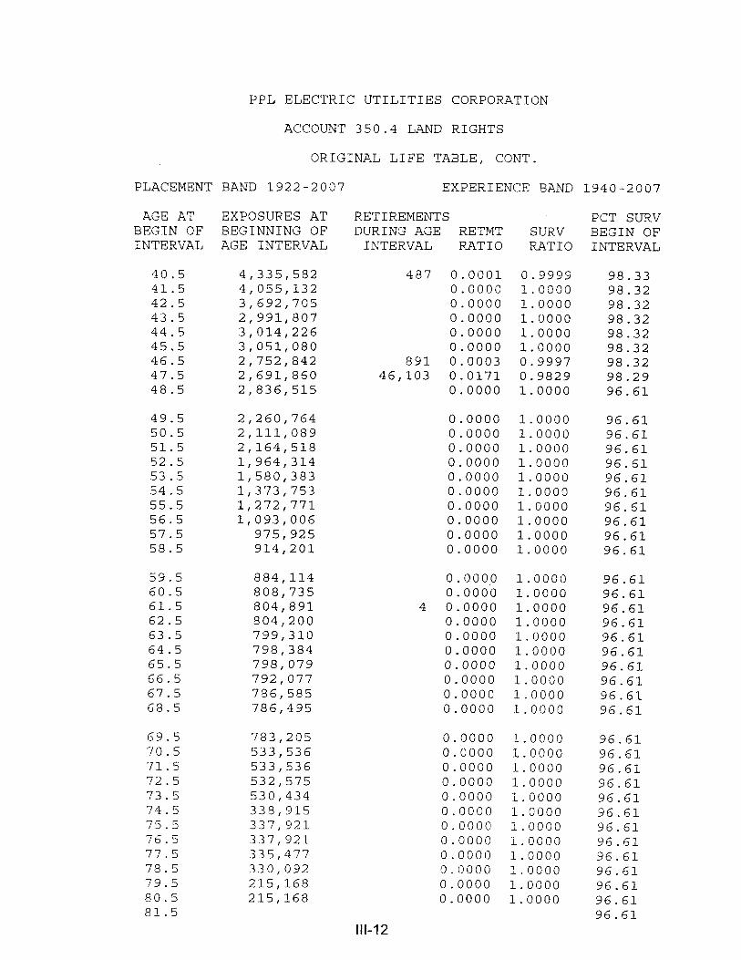
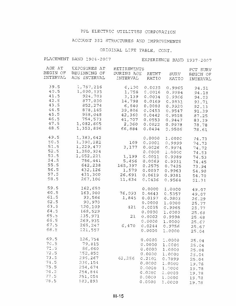
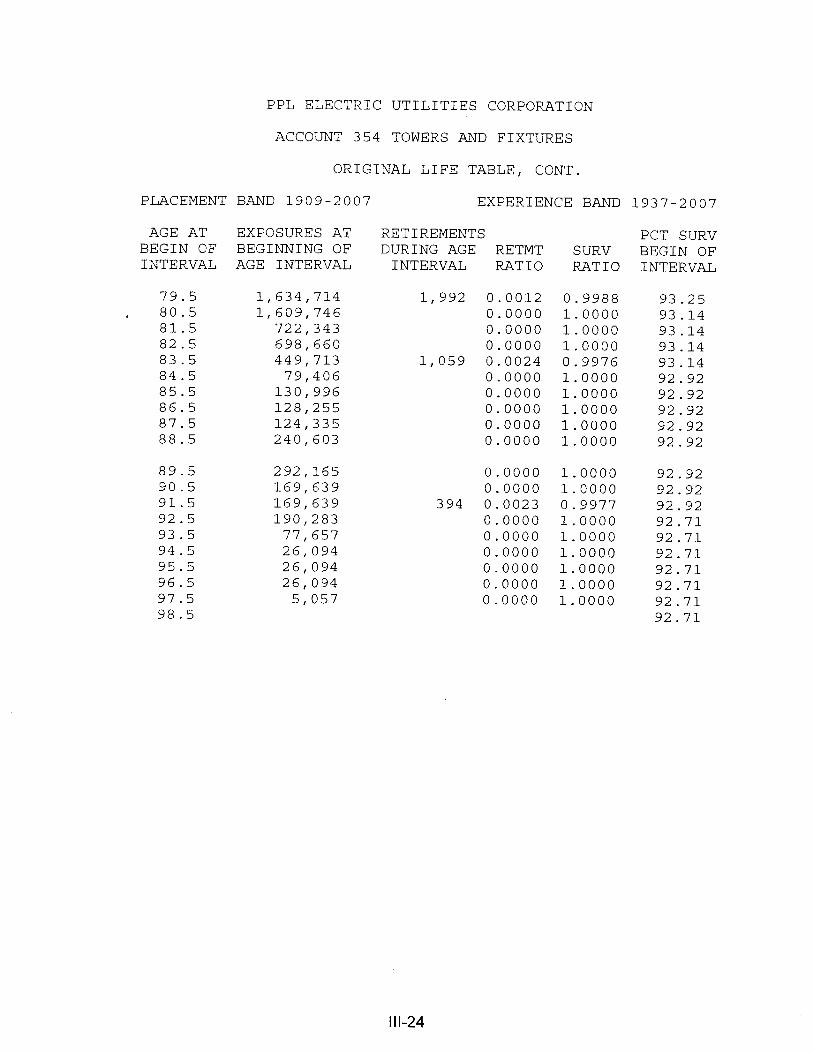
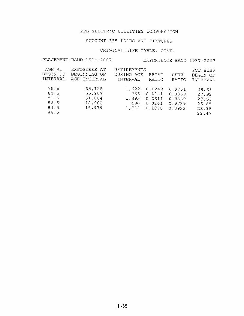
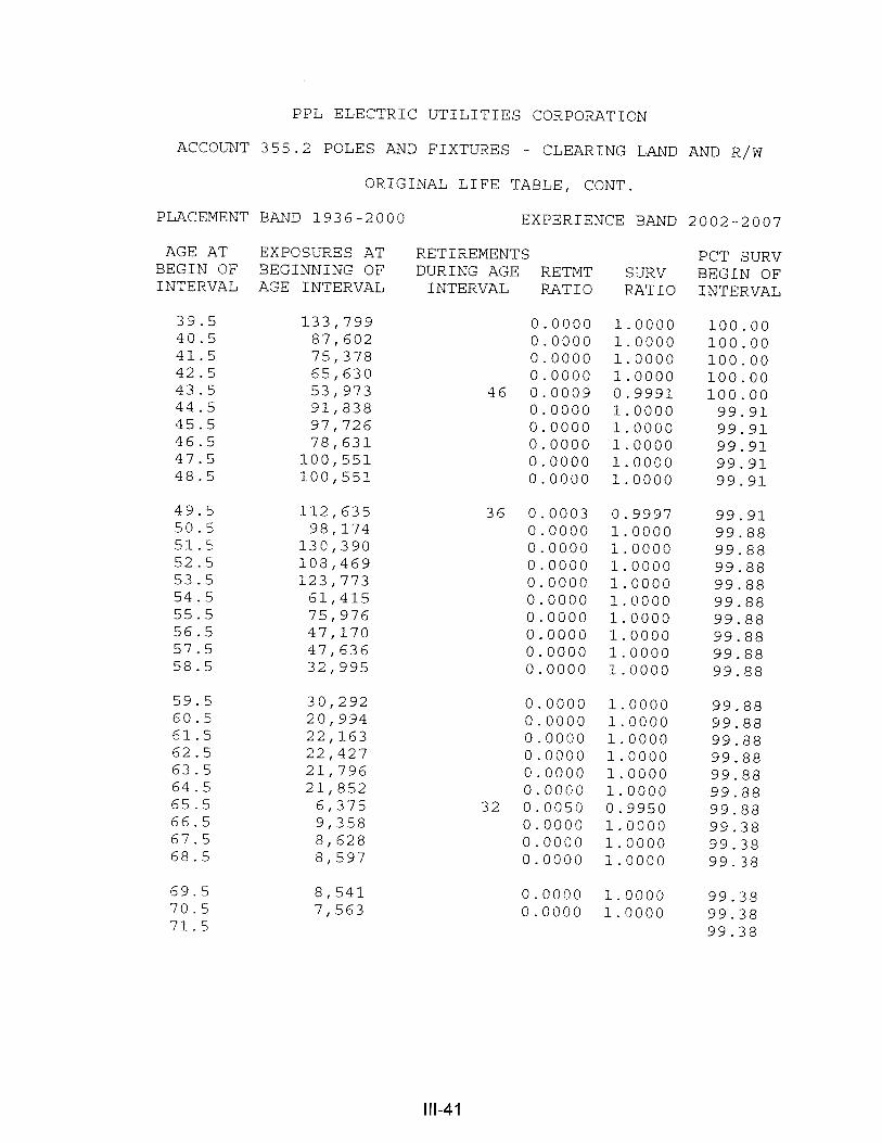
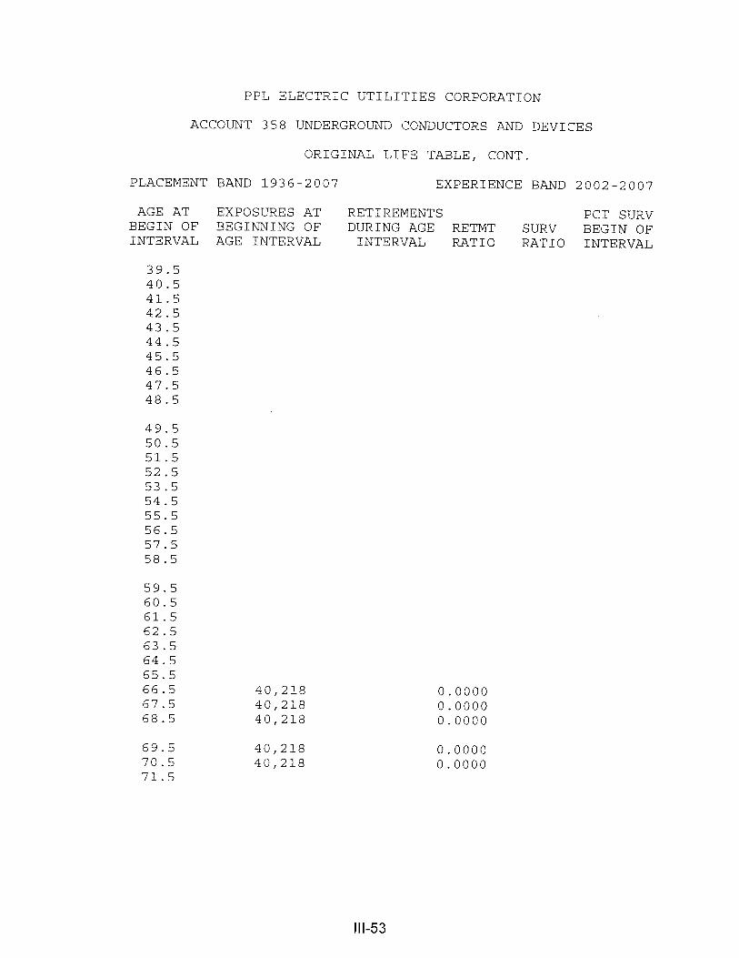
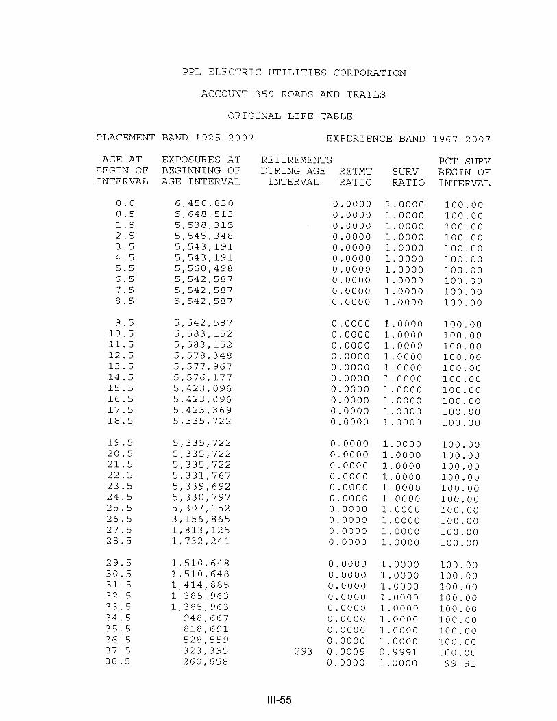
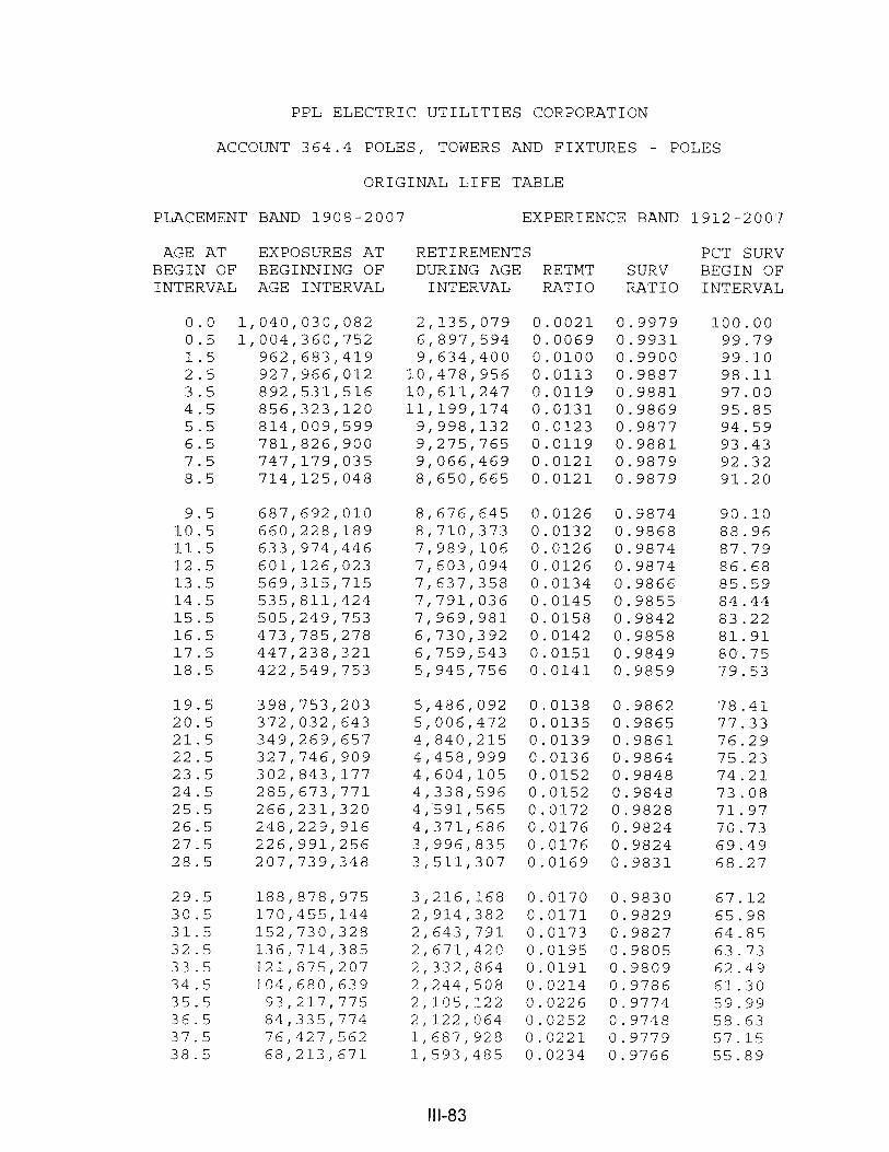
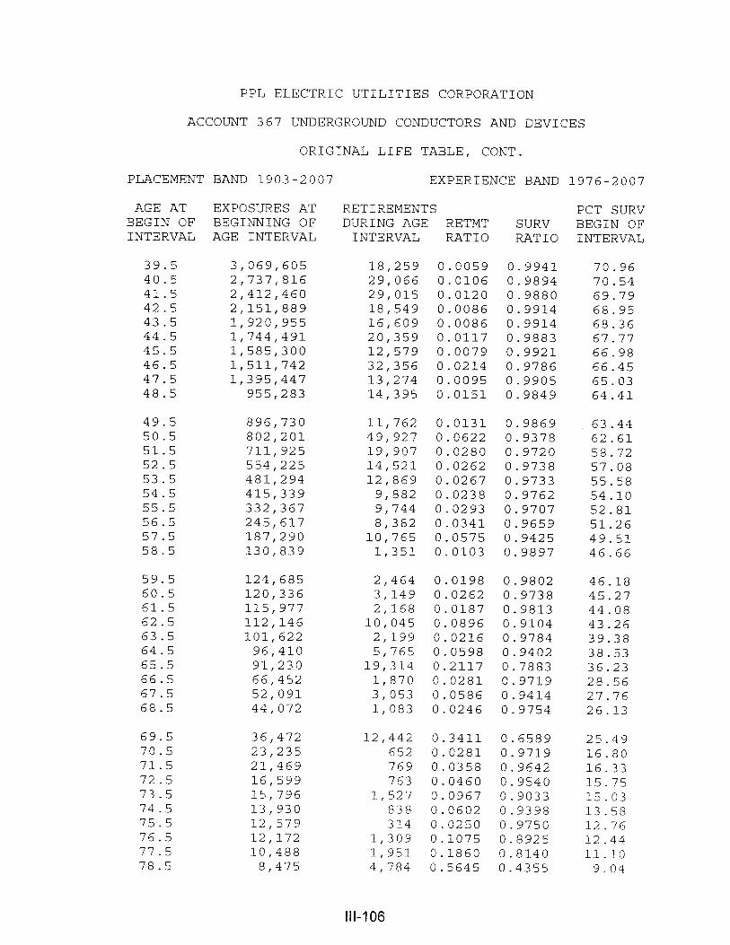
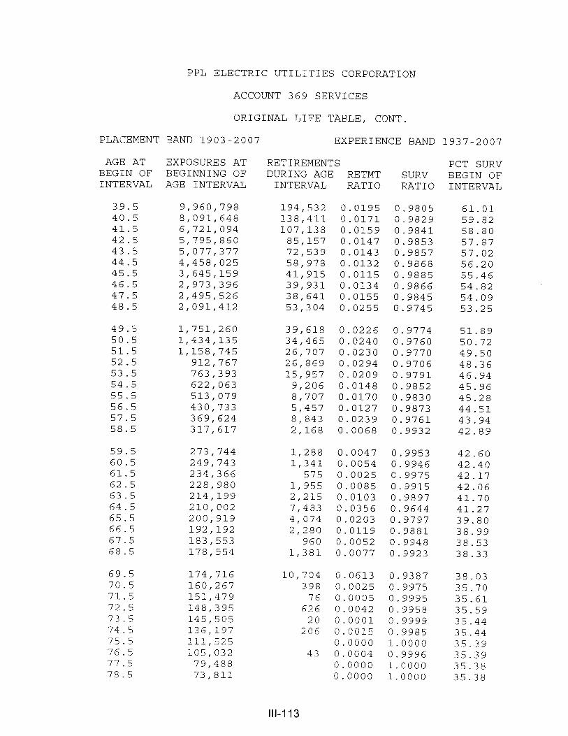
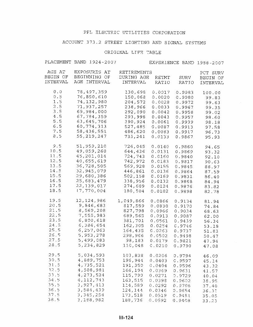
Original Life Table. The original life table, illustrated in Schedule 4 on page II-18,

is developed from the totals shown on the schedules of retirements and exposures,

Schedules 1 and 3, respectively. The exposures at the beginning of the age interval are

obtained from the corresponding age interval of the exposure schedule, and the retirements

during the age interval are obtained from the corresponding age interval of the retirement

schedule. The retirement ratio is the result of dividing the retirement during the age interval

by the exposures at the beginning of the age interval. The percent surviving at the

beginning of each age interval is derived from survivor ratios, each of which equals one

minus the retirement ratio. The percent surviving is developed by starting with 100% at age

zero and successively multiplying the percent surviving at the beginning of each interval

by the survivor ratio, i.e., one minus the retirement ratio for that age interval. The

calculations necessary to determine the percent surviving at age 5½ are as follows:

Percent surviving at age 4½ = 88.15 Exposures at age 4½ = 3,789,000Retirements from age 4½ to 5½ = 143,000 Retirement Ratio = 143,000 ÷ 3,789,000 = 0.0377Survivor Ratio = 1.000 - 0.0377 = 0.9623Percent surviving at age 5½ = (88.15) x (0.9623) = 84.83

II-18

SCHEDULE 4. ORIGINAL LIFE TABLECALCULATED BY THE RETIREMENT RATE METHOD

Experience Band 2002-2011 Placement Band 1997-2011

(Exposure and Retirement Amounts are in Thousands of Dollars)

Age atBeginning of Interval

Exposures atBeginning of

Age Interval

RetirementsDuring Age Interval

Retirement Ratio

Survivor Ratio

PercentSurviving atBeginning ofAge Interval

(1) (2) (3) (4) (5) (6)

0.0 7,490 80 0.0107 0.9893 100.00 0.5 6,579 153 0.0233 0.9767 98.93 1.5 5,719 151 0.0264 0.9736 96.62 2.5 4,955 150 0.0303 0.9697 94.07 3.5 4,332 146 0.0337 0.9663 91.22 4.5 3,789 143 0.0377 0.9623 88.15 5.5 3,057 131 0.0429 0.9571 84.83 6.5 2,463 124 0.0503 0.9497 81.19 7.5 1,952 113 0.0579 0.9421 77.11 8.5 1,503 105 0.0699 0.9301 72.65 9.5 1,097 93 0.0848 0.9152 67.57

10.5 823 83 0.1009 0.8991 61.84 11.5 531 64 0.1205 0.8795 55.60 12.5 323 44 0.1362 0.8638 48.90 13.5 167 26 0.1557 0.8443 42.24

35.66 Total 44,780 1,606

Column 2 from Schedule 3, Column 12, Plant Exposed to Retirement.Column 3 from Schedule 1, Column 12, Retirements for Each Year.Column 4 = Column 3 Divided by Column 2.Column 5 = 1.0000 Minus Column 4.Column 6 = Column 5 Multiplied by Column 6 as of the Preceding Age Interval.

II-19

The totals of the exposures and retirements (columns 2 and 3) are shown for the

purpose of checking with the respective totals in Schedules 1 and 3. The ratio of the total

retirements to the total exposures, other than for each age interval, is meaningless.

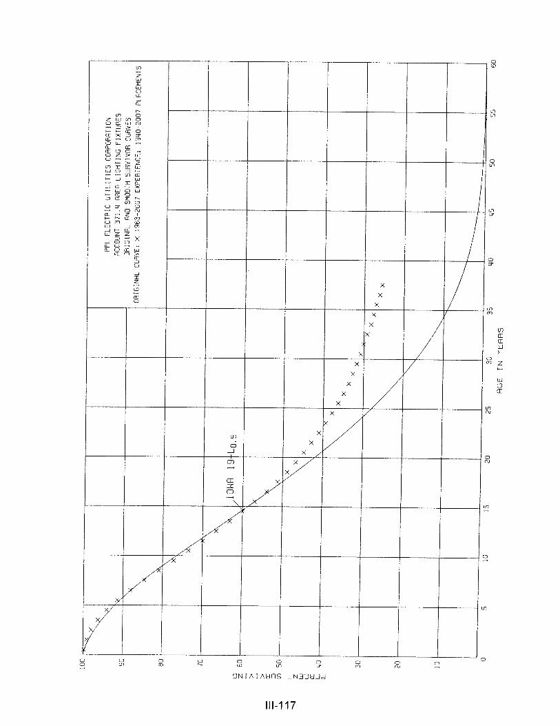
The original survivor curve is plotted from the original life table (column 6, Schedule

4). When the curve terminates at a percent surviving greater than zero, it is called a stub

survivor curve. Survivor curves developed from retirement rate studies generally are stub

curves.

Smoothing the Original Survivor Curve. The smoothing of the original survivor curve

eliminates any irregularities and serves as the basis for the preliminary extrapolation to zero

percent surviving of the original stub curve. Even if the original survivor curve is complete

from 100% to zero percent, it is desirable to eliminate any irregularities as there is still an

extrapolation for the vintages which have not yet lived to the age at which the curve reaches

zero percent. In this study, the smoothing of the original curve with established type curves

was used to eliminate irregularities in the original curve.

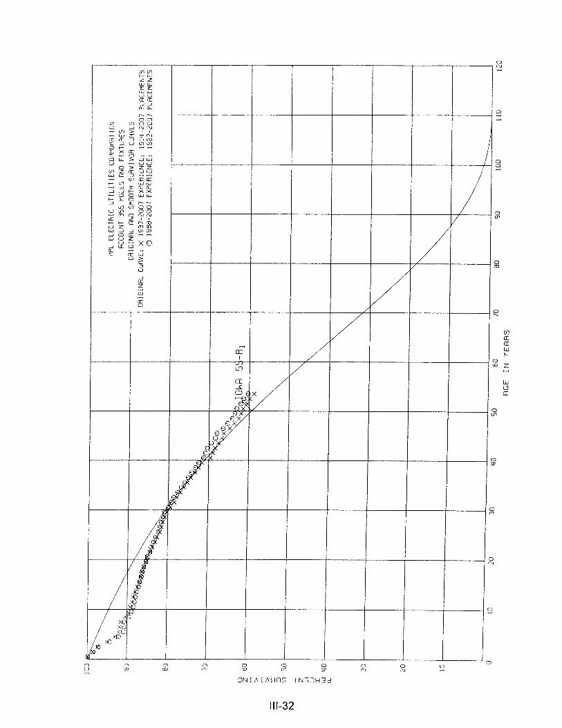
The Iowa type curves are used in this study to smooth those original stub curves

which are expressed as percents surviving at ages in years. Each original survivor curve

was compared to the Iowa curves using visual and mathematical matching in order to

determine the better fitting smooth curves. In Figures 6, 7, and 8, the original curve

developed in Schedule 4 is compared with the L, S, and R Iowa type curves which most

nearly fit the original survivor curve. In Figure 6, the L1 curve with an average life between

12 and 13 years appears to be the best fit. In Figure 7, the S0 type curve with a 12-year

average life appears to be the best fit and appears to be better than the L1 fitting. In Figure

8, the R1 type curve with a 12-year average life appears to be the best fit and appears to

be better than either the L1 or the S0. In Figure 9, the three fittings, 12-L1, 12-S0, and 12-

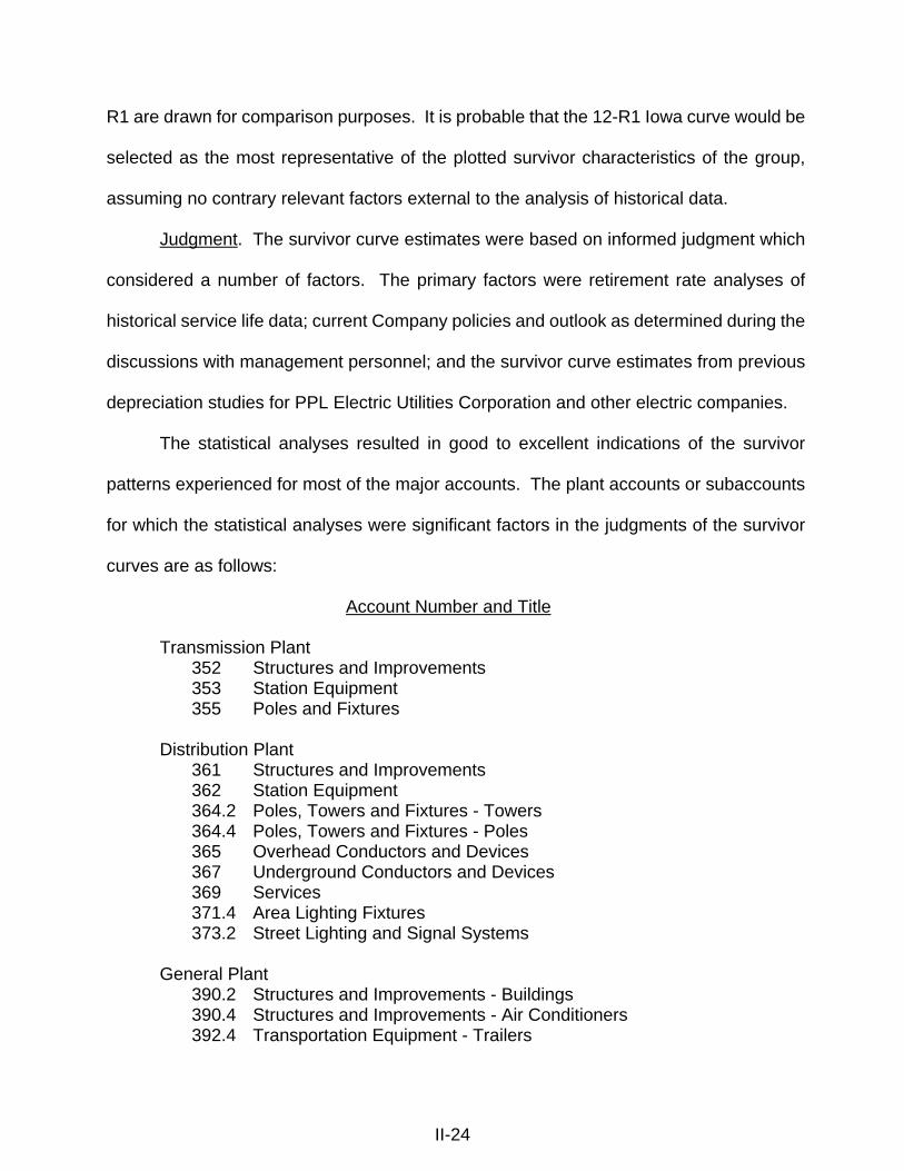
II-24

R1 are drawn for comparison purposes. It is probable that the 12-R1 Iowa curve would be

selected as the most representative of the plotted survivor characteristics of the group,

assuming no contrary relevant factors external to the analysis of historical data.

Judgment. The survivor curve estimates were based on informed judgment which

considered a number of factors. The primary factors were retirement rate analyses of

historical service life data; current Company policies and outlook as determined during the

discussions with management personnel; and the survivor curve estimates from previous

depreciation studies for PPL Electric Utilities Corporation and other electric companies.

The statistical analyses resulted in good to excellent indications of the survivor

patterns experienced for most of the major accounts. The plant accounts or subaccounts

for which the statistical analyses were significant factors in the judgments of the survivor

curves are as follows:

Account Number and Title

Transmission Plant352 Structures and Improvements353 Station Equipment355 Poles and Fixtures

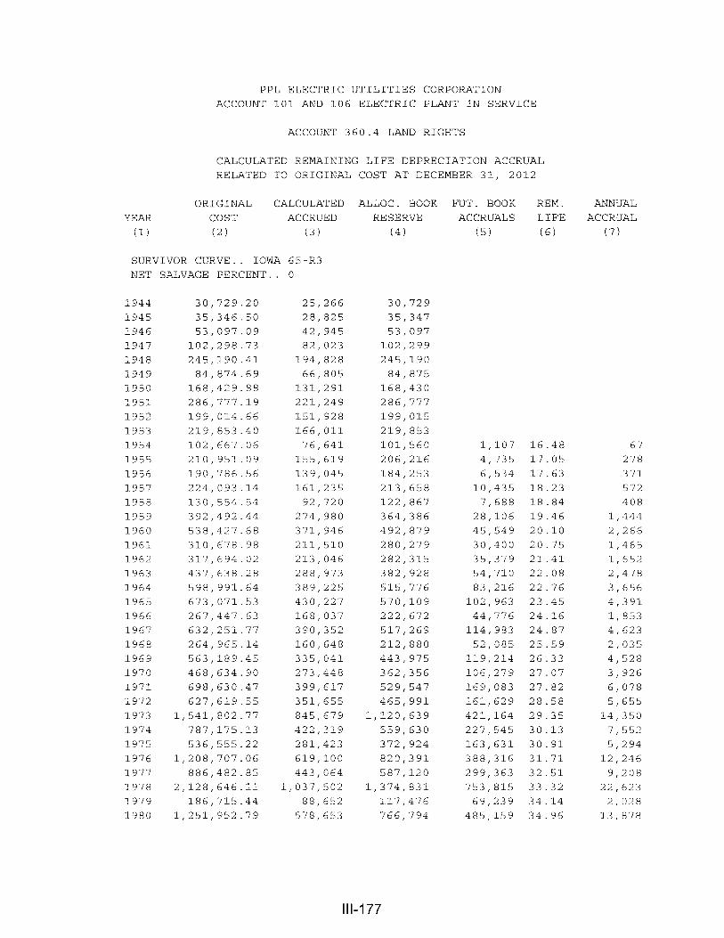
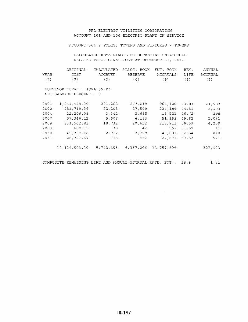
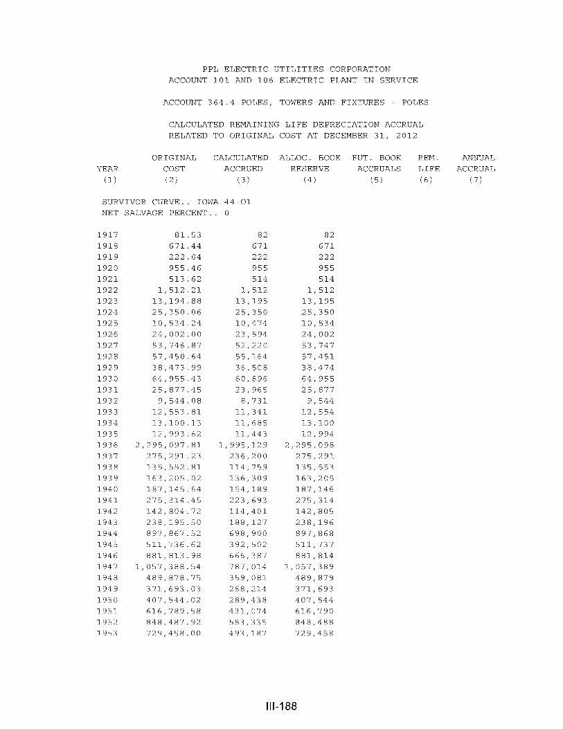
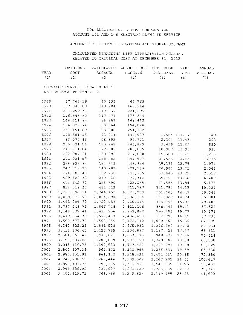
Distribution Plant361 Structures and Improvements362 Station Equipment364.2 Poles, Towers and Fixtures - Towers364.4 Poles, Towers and Fixtures - Poles365 Overhead Conductors and Devices367 Underground Conductors and Devices369 Services 371.4 Area Lighting Fixtures373.2 Street Lighting and Signal Systems

General Plant390.2 Structures and Improvements - Buildings390.4 Structures and Improvements - Air Conditioners392.4 Transportation Equipment - Trailers

II-25

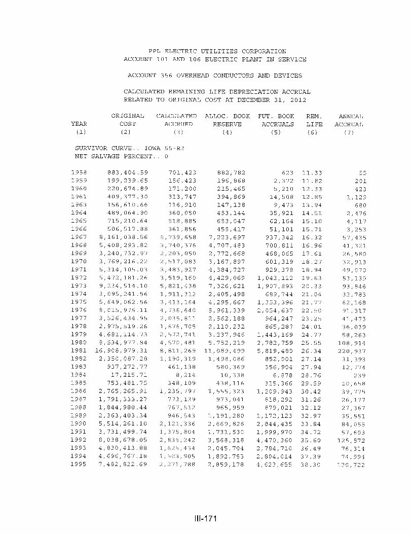
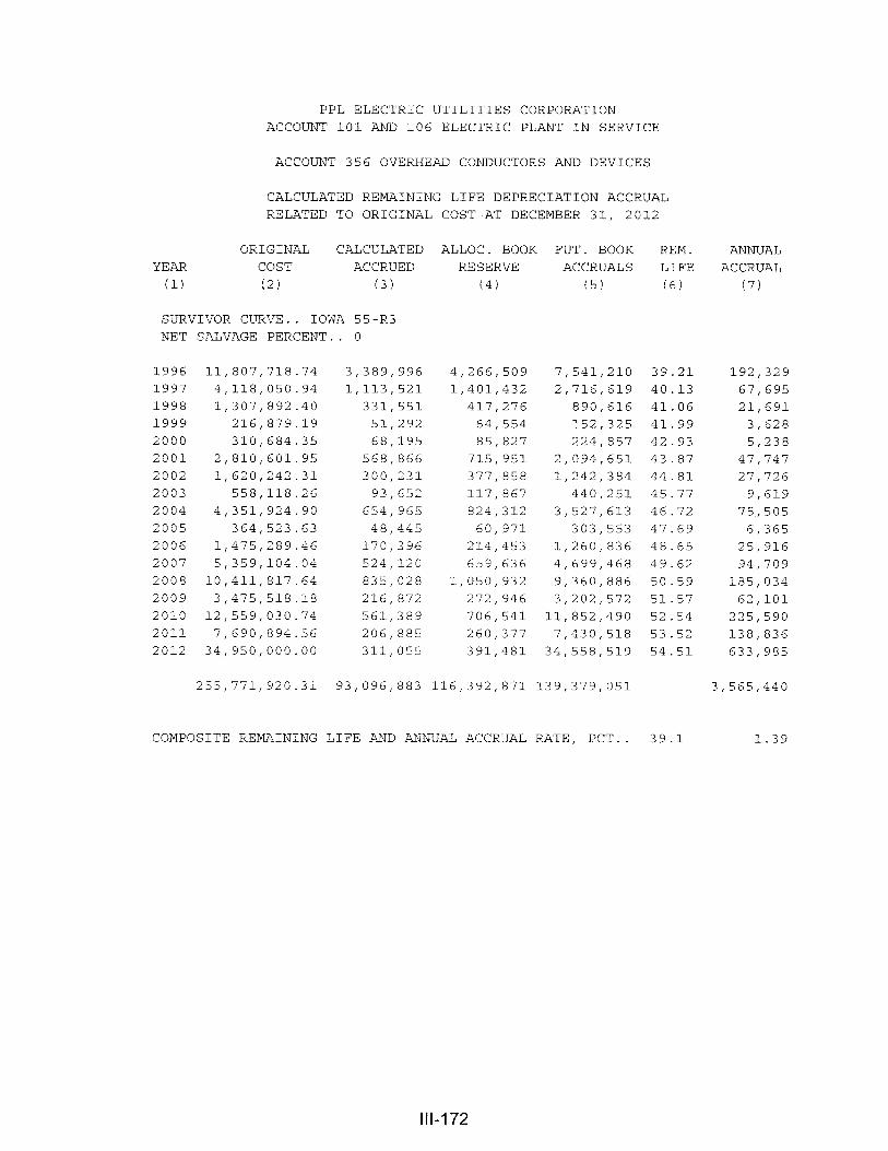
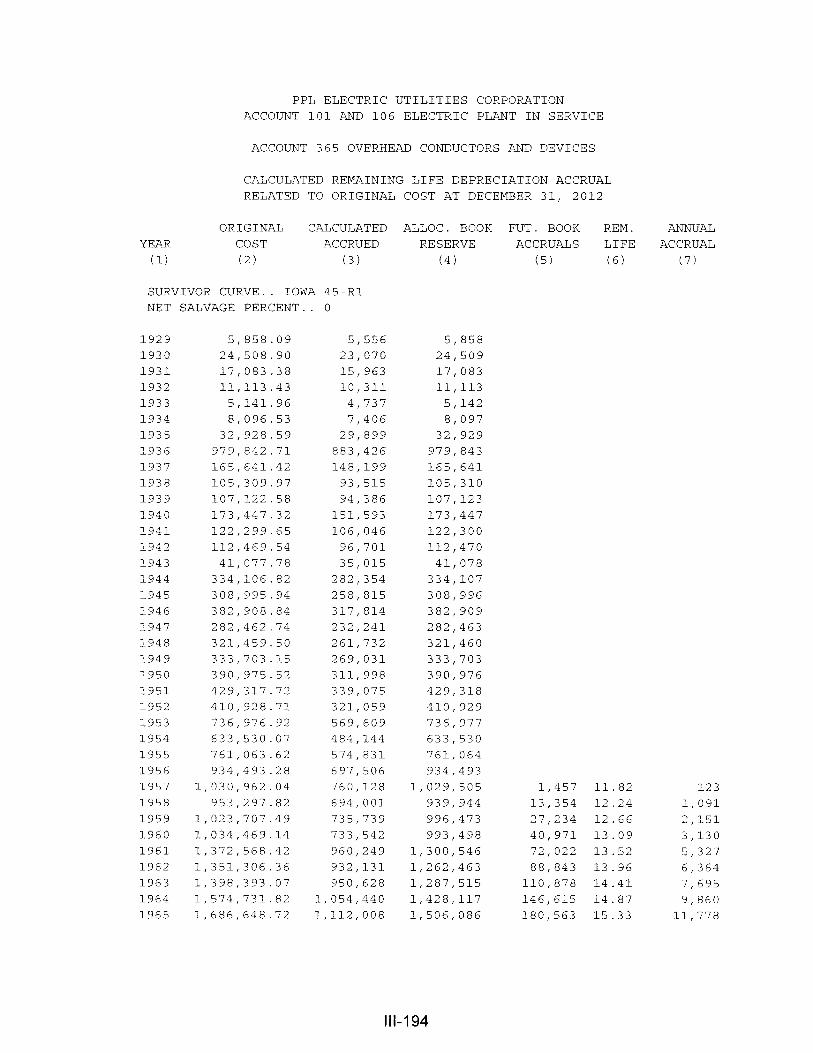
Account 365, Overhead Conductors and Devices, is used to illustrate the manner

in which the study was conducted for the groups in the preceding list. It is a significant

account and serves as a typical illustration. Aged plant accounting data have been

compiled for the years 1912 through 2007. These data were coded by type of transaction,

year in which the transaction took place, and year in which the plant was placed in service.

The data were analyzed by the retirement rate method to obtain an indication of the

experienced service life characteristics.

The estimated Iowa 45-R1 survivor curve is based on the experience band, 1912

through 2007. The estimated survivor curve is an excellent fit of the observed data, is

similar to the previous estimates for this account, and is within the typical range of lives

used by the electric utility industry.

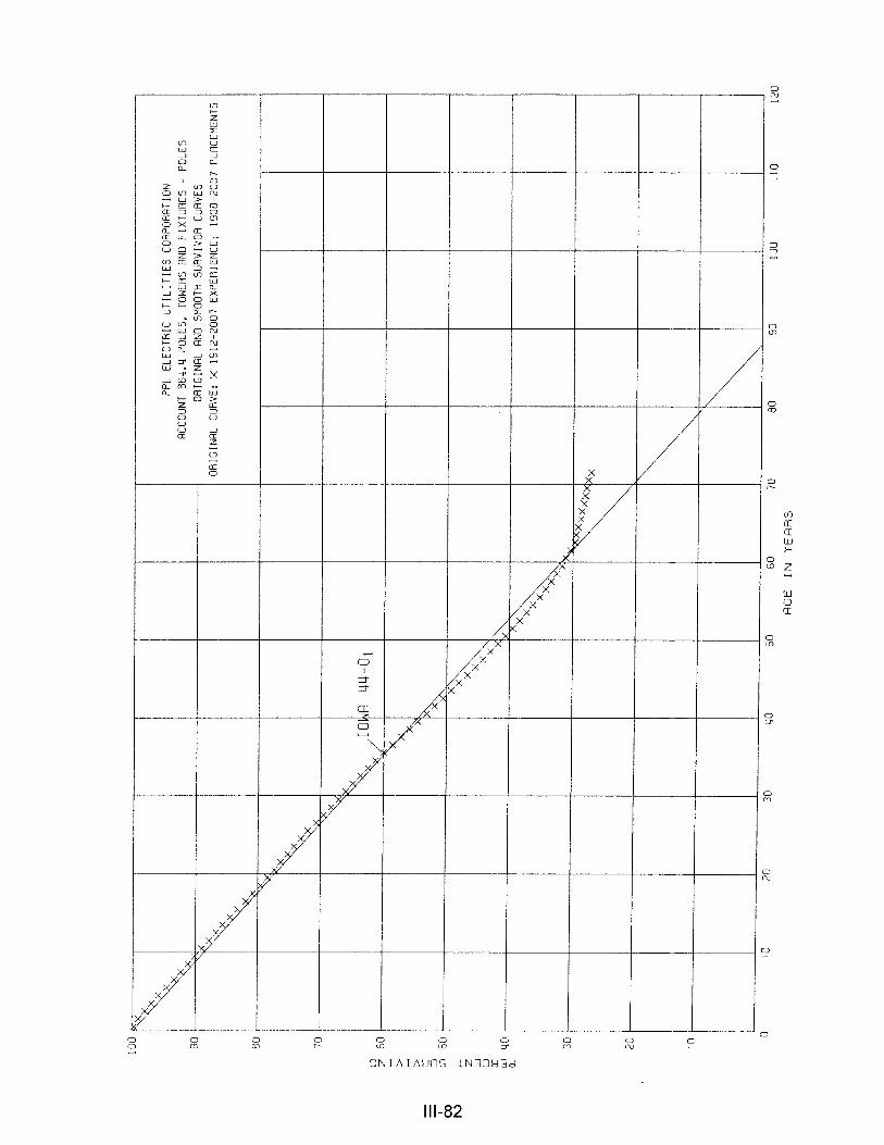
For Account 364.4, Poles, Towers and Fixtures - Poles, the estimate of survivor

characteristics is based on the 1912-2007 experience band. Most retirements have been

due to wear and tear. Typical service lives for poles and fixtures range from 30 to 50 years.

Most of the poles included in this account are wood poles. Wood poles are a natural

product subject to decay and rot. The climate and pole treatment are the predominant

factors regarding the service life of wood poles. This is the reason for the wide range of

lives experienced within the industry. During the past 20 years, PPL Electric Utilities

Corporation has embarked on a change to the pole treatment plan in order to maintain a

reasonable service lives of poles. The Iowa 40-R0.5 survivor curve reflects the outlook of

management, is within the range of estimates used by other utilities and is a reasonable

interpretation of a significant portion of the survivor curve through age 63.

II-26

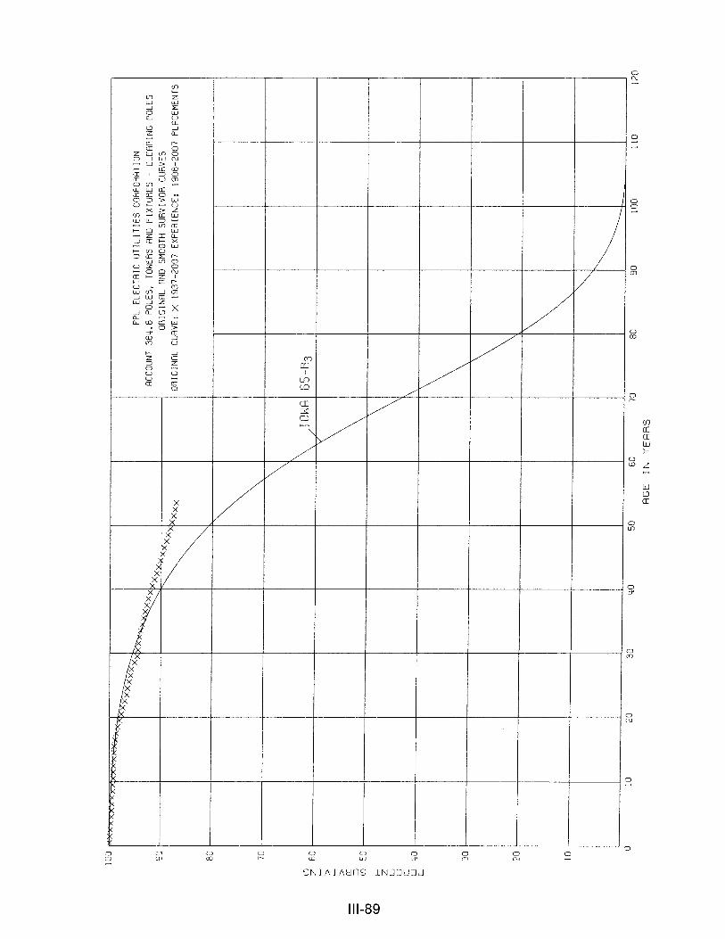
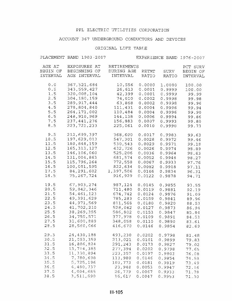
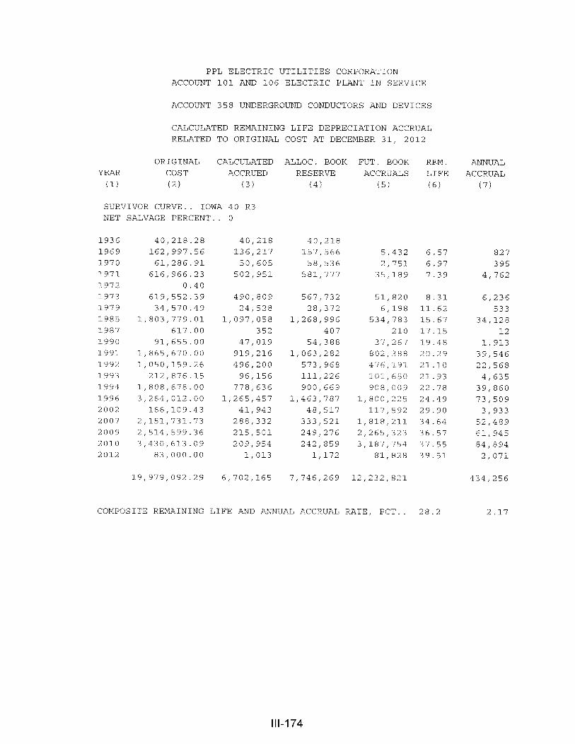
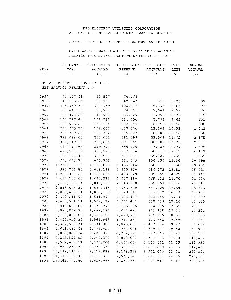
The estimate for Account 367, Underground Conductors and Devices, the 43-S1.5,

is based on management's expectation of a relatively short life for the direct buried

conductor which represents a significant portion of the conductor in this account. Most of

the remaining direct buried conductor included in this account was added between the early

1970's and 1983. The Company has an active program in place to remove the remaining

investment of direct buried conductor. Management’s expectation of retirements to be high

for the next five to ten years is reflected in the 43 year average service life.

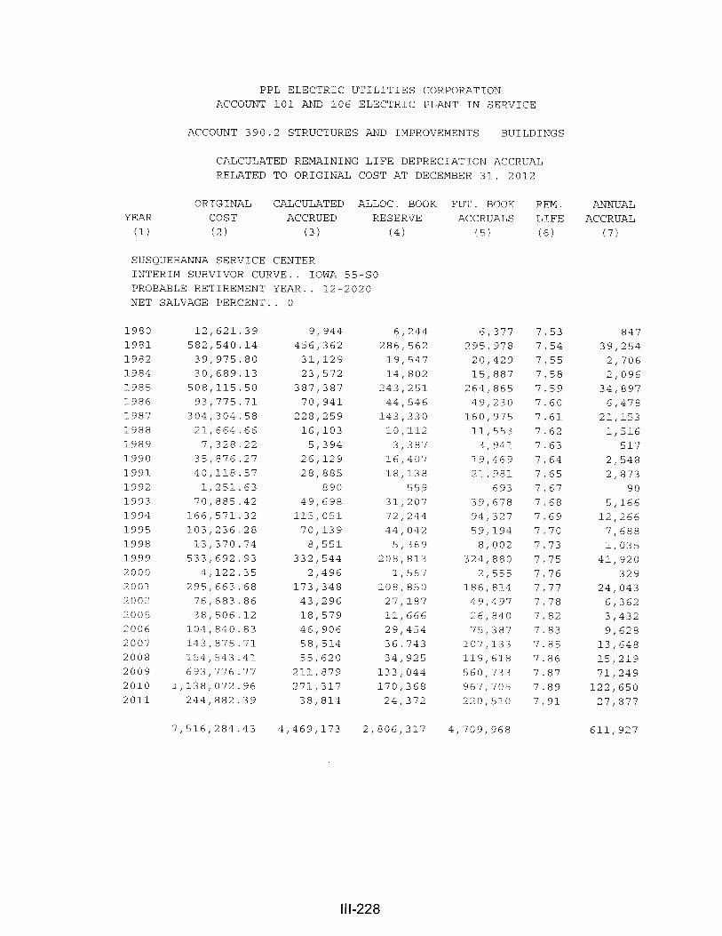
The life span technique also was used for large office buildings and service centers

in Account 390.2, Structures and Improvements - Buildings - Major. For these large

structures in Account 390.2, a life span was estimated for each structure based on its type

of construction, use, age, condition and management's plans within the foreseeable future.

In Account 390.2, Structures and Improvements - Buildings - Major, an interim survivor

curve was estimated for each location, since interim retirements are normal for such

structures and, in fact, have been experienced.

Generally, the survivor curve estimates for the remainder of the accounts were

based on engineering judgment, considering the nature of the plant and equipment, review

of available historical retirement data and a general knowledge of the service lives for

similar equipment in other electric companies.

CALCULATION OF ANNUAL AND ACCRUED DEPRECIATION

Group Depreciation Procedures. A group procedure for depreciation is appropriate

when considering more than a single item of property. Normally, the items within a group

do not have identical service lives, but have lives that are dispersed over a range of time.

In the average service life procedure, the rate of annual depreciation is based on the

average life or average remaining life of the group, and this rate is applied to the surviving

II-27

Ratio = 1 - Average Remaining LifeAverage Service Life

.

balances of the group's cost. A characteristic of this procedure is that the cost of plant

retired prior to average life is not fully recouped at the time of retirement, whereas the cost

of plant retired subsequent to average life is more than fully recouped. Over the entire life

cycle, the portion of cost not recouped prior to average life is balanced by the cost

recouped subsequent to average life.

Remaining Life Annual Accruals. For the purpose of calculating remaining life

accrual rates as of December 31, 2012, the estimated book depreciation reserve for each

plant account is allocated among vintages in proportion to the calculated accrued

depreciation for the account. Explanations of remaining life accruals and accrued

depreciation calculated by the average service life procedure follow. The detailed

calculations are set forth in the Results of Study section of the report.

Average Service Life Procedure. In the average service life procedure, the

remaining life annual accrual for each vintage is determined by dividing future book

accruals (original cost less book reserve) by the average remaining life of the vintage. The

average remaining life is a directly-weighted average derived from the estimated future

survivor curve in accordance with the average service life procedure.

The calculated accrued depreciation for each depreciable property group represents

that portion of the depreciable cost of the group which would not be allocated to expense

through future whole life depreciation accruals if current forecasts of life characteristics are

used as the basis for such accruals. The accrued depreciation calculation consists of

applying an appropriate ratio to the surviving original cost of each vintage of each account,

based upon the attained age and service life. The straight line accrued depreciation ratios

are calculated as follows for the average service life procedure.

II-28

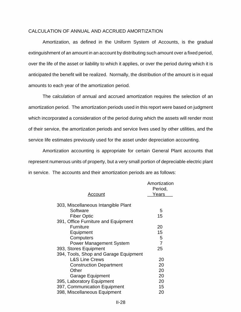
CALCULATION OF ANNUAL AND ACCRUED AMORTIZATION

Amortization, as defined in the Uniform System of Accounts, is the gradual

extinguishment of an amount in an account by distributing such amount over a fixed period,

over the life of the asset or liability to which it applies, or over the period during which it is

anticipated the benefit will be realized. Normally, the distribution of the amount is in equal

amounts to each year of the amortization period.

The calculation of annual and accrued amortization requires the selection of an

amortization period. The amortization periods used in this report were based on judgment

which incorporated a consideration of the period during which the assets will render most

of their service, the amortization periods and service lives used by other utilities, and the

service life estimates previously used for the asset under depreciation accounting.

Amortization accounting is appropriate for certain General Plant accounts that

represent numerous units of property, but a very small portion of depreciable electric plant

in service. The accounts and their amortization periods are as follows:

Amortization Period, Account Years

303, Miscellaneous Intangible Plant Software 5 Fiber Optic 15

391, Office Furniture and Equipment Furniture 20 Equipment 15 Computers 5 Power Management System 7

393, Stores Equipment 25394, Tools, Shop and Garage Equipment

L&S Line Crews 20 Construction Department 20 Other 20 Garage Equipment 20

395, Laboratory Equipment 20397, Communication Equipment 15398, Miscellaneous Equipment 20

II-29

For the purpose of calculating annual amortization amounts as of December 31,

2012, the book depreciation reserve for each plant account or subaccount is assigned or

allocated to vintages. The book reserve assigned to vintages with an age greater than the

amortization period is equal to the vintage's original cost. The remaining book reserve is

allocated among vintages with an age less than the amortization period in proportion to the

calculated accrued amortization. The calculated accrued amortization is equal to the

original cost multiplied by the ratio of the vintage's age to its amortization period. The

annual amortization amount is determined by dividing the future amortizations (original cost

less allocated book reserve) by the remaining period of amortization for the vintage.

III-2


QUALIFICATION OF RESULTS

The calculated annual depreciation accrual rates are the principal results of the

study. Continued surveillance and periodic revisions are normally required to maintain

continued use of appropriate annual depreciation accrual rates. An assumption that

accrual rates can remain unchanged over a long period of time implies a disregard for the

inherent variability in service lives and salvage and for the change of the composition of

property in service. The annual accrual rates were calculated in accordance with the

straight line remaining life method of depreciation using the average service life procedure

based on estimates which reflect considerations of current historical evidence and expected

future conditions.

The annual depreciation accrual rates are applicable specifically to the electric plant

in service as of December 31, 2012. For most plant accounts, the application of such rates

to future balances that reflect additions subsequent to December 31, 2012, is reasonable

for a period of three to five years.

DESCRIPTION OF STATISTICAL SUPPORT

The service life and salvage estimates were based on judgment which incorporated

statistical analyses of retirement data, discussions with management and consideration of

estimates made for other electric utility companies. The results of the statistical analyses

of service life are presented in the section titled, “Service Life Statistics”.

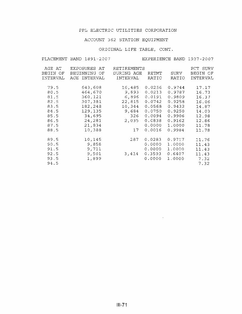
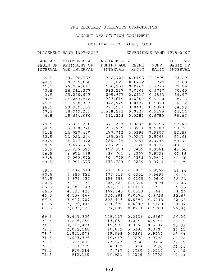
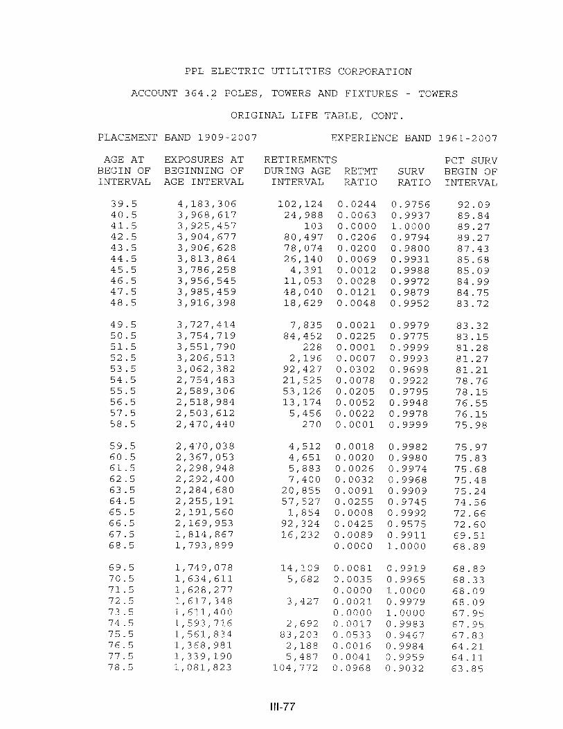
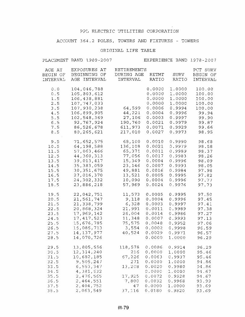
The estimated survivor curves for each account are presented in graphical form.

The charts depict the estimated smooth survivor curve and original survivor curve(s), when

applicable, related to each specific group. For groups where the original survivor curve was

plotted, the calculation of the original life table is also presented.

III-3

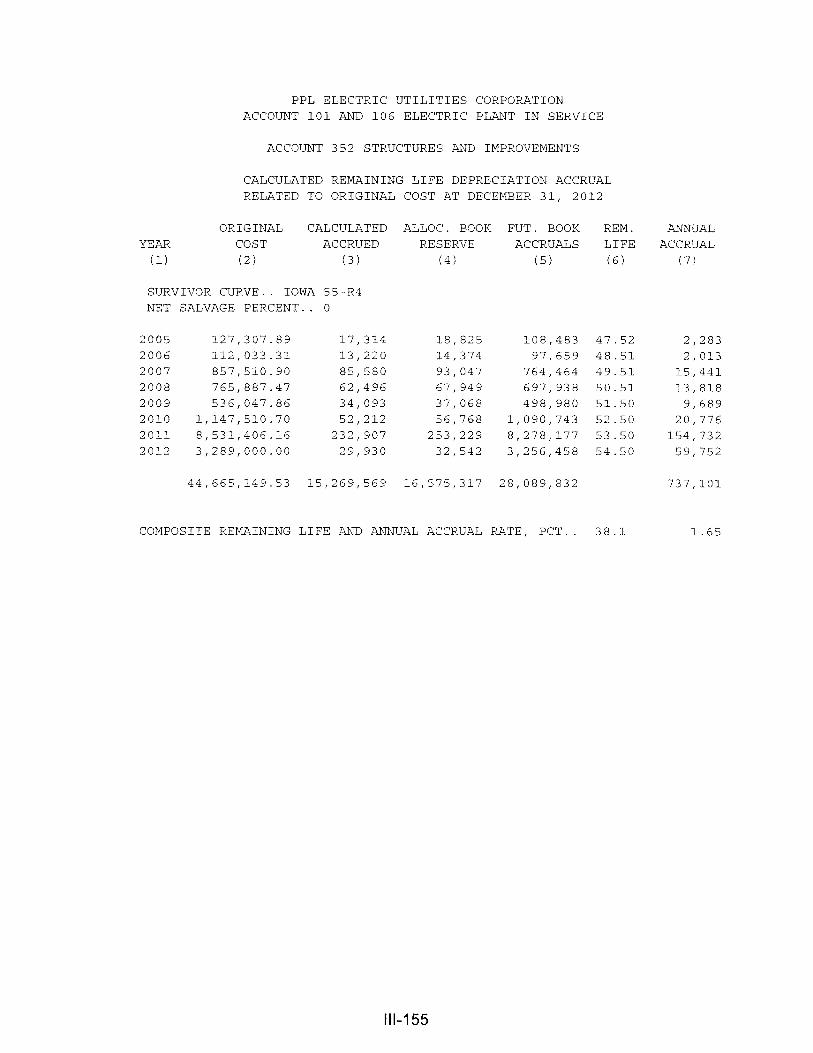
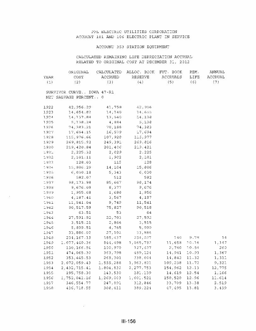
DESCRIPTION OF DEPRECIATION TABULATIONS

The summary tables of the results of the study, as applied to the original cost of

electric plant as of December 31, 2012, are presented on pages III-4 through III-8 of this

report. Table 1 sets forth the original cost, the book reserve, future accruals, the calculated

annual depreciation rate and amount, and the composite remaining life related to electric

plant. Table 2 sets forth the development of the book reserve from December 31, 2011 to

December 31, 2012. Table 3 establishes the amortization of net salvage by function for the

five-year period, 2008-2012.

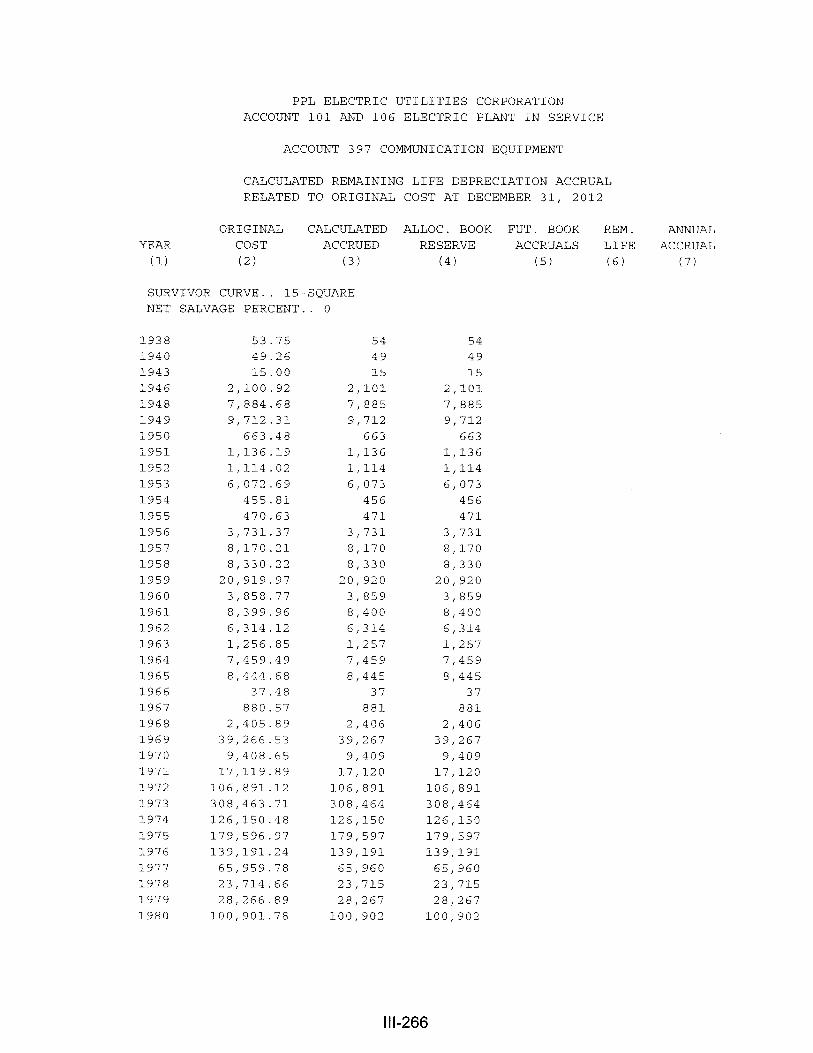
The tables of the calculated annual depreciation accruals are presented in account

sequence in the section titled “Depreciation Calculations.” The tables indicate the

estimated survivor curve and salvage percent for the account and set forth, for each

installation year, the original cost, the calculated accrued depreciation, the allocated book

reserve, future accruals, the remaining life and the calculated annual accrual amount.

ppl electric utilities corporation exhibit … as used in accounting, is a method of distributing...

Documents