Pre-processing in DNA microarray experiments

Sandrine Dudoit

PH 296, Section 33

13/09/2001

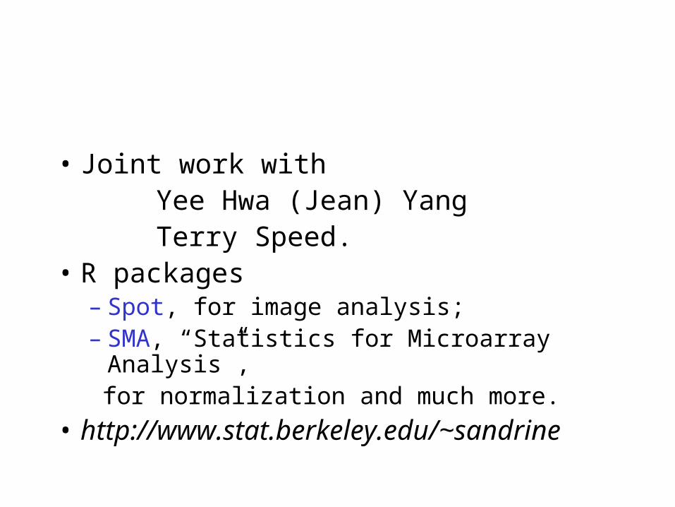
• Joint work with Yee Hwa (Jean) Yang Terry Speed.• R packages

– Spot, for image analysis;– SMA, “Statistics for Microarray Analysis”, for normalization and much more.

• http://www.stat.berkeley.edu/~sandrine

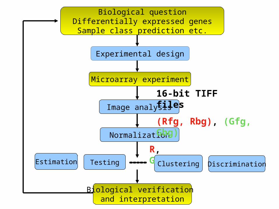
Biological questionDifferentially expressed genesSample class prediction etc.

Testing

Biological verification and interpretation

Microarray experiment

Estimation

Experimental design

Image analysis

Normalization

Clustering Discrimination

R, G

16-bit TIFF files

(Rfg, Rbg), (Gfg, Gbg)

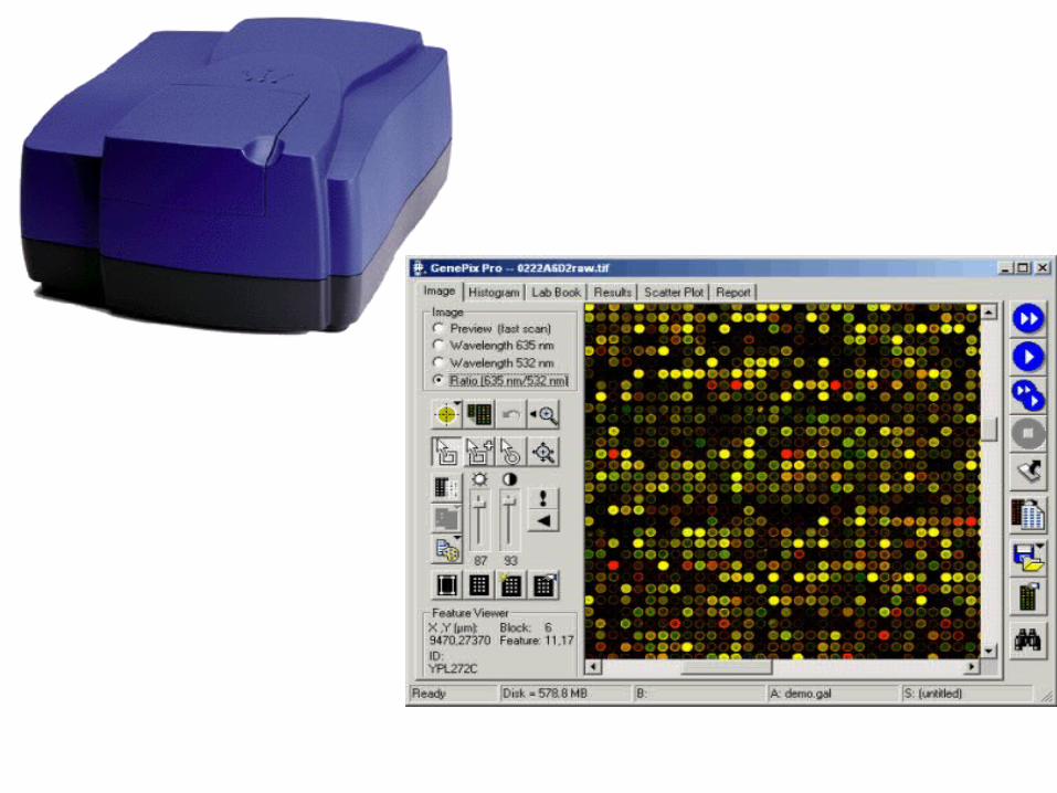
Image analysis

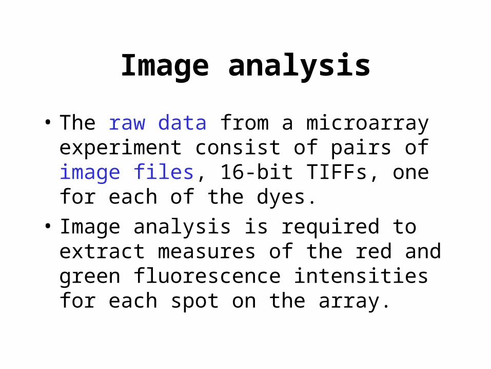
Image analysis

• The raw data from a microarray experiment consist of pairs of image files, 16-bit TIFFs, one for each of the dyes.

• Image analysis is required to extract measures of the red and green fluorescence intensities for each spot on the array.

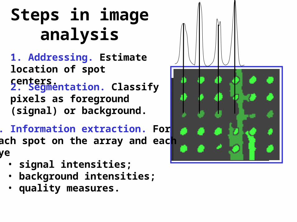
Steps in image analysis

1. Addressing. Estimate location of spot centers.

2. Segmentation. Classify pixels as foreground (signal) or background.

3. Information extraction. For each spot on the array and each dye

• signal intensities;• background intensities; • quality measures.

Spot• Software package. Spot, built on the freely available

software package R.

• Batch automatic addressing.• Segmentation. Seeded region growing (Adams & Bischof

1994): adaptive segmentation method, no restriction on the size or shape of the spots.

• Information extraction– Foreground. Mean of pixel intensities within a spot.– Background. Morphological opening: non-linear filter

which generates an image of the estimated background intensity for the entire slide.

• Spot quality measures.

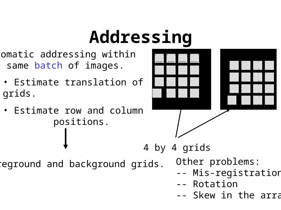
Addressing

4 by 4 grids

Automatic addressing within the same batch of images.

Other problems:-- Mis-registration-- Rotation-- Skew in the array

• Estimate translation of grids.

• Estimate row and column positions.

Foreground and background grids.

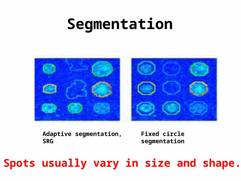
Segmentation

Adaptive segmentation, SRG Fixed circle segmentation

Spots usually vary in size and shape.

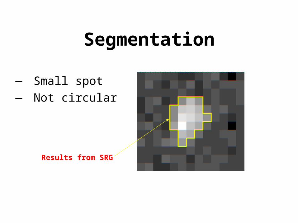
Segmentation

— Small spot— Not circular

Results from SRG

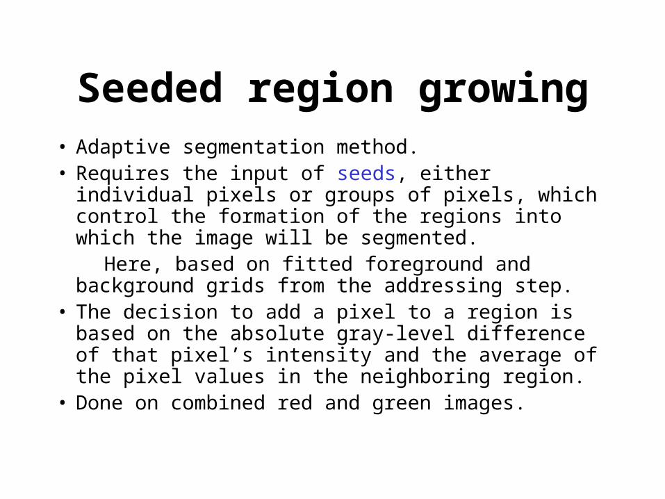
Seeded region growing• Adaptive segmentation method.• Requires the input of seeds, either individual pixels or

groups of pixels, which control the formation of the regions into which the image will be segmented.

Here, based on fitted foreground and background grids from the addressing step.

• The decision to add a pixel to a region is based on the absolute gray-level difference of that pixel’s intensity and the average of the pixel values in the neighboring region.

• Done on combined red and green images.

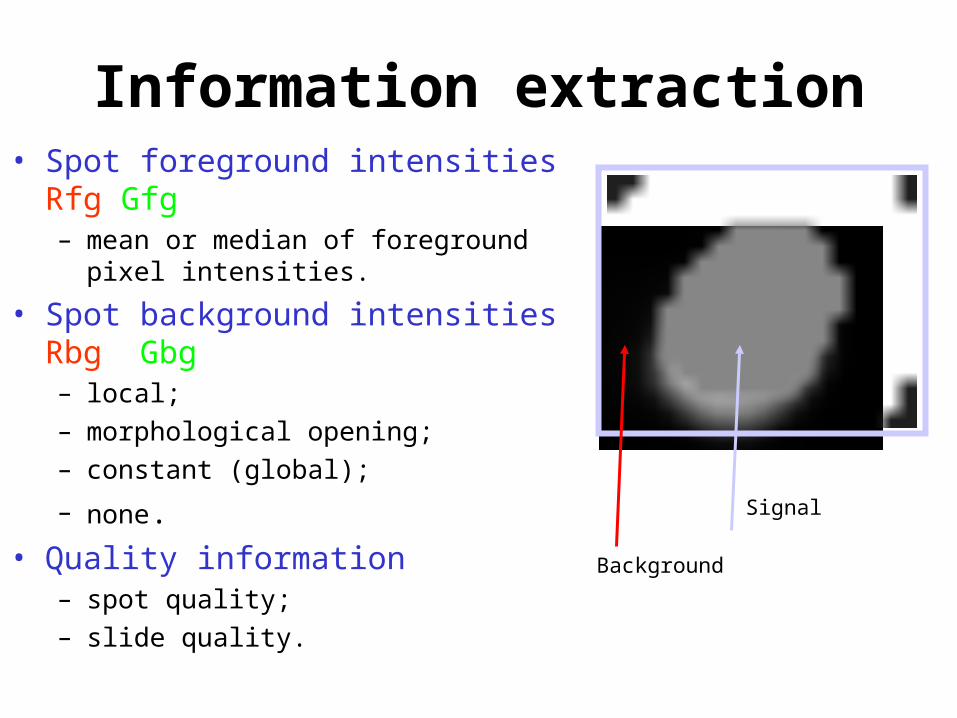
Information extraction• Spot foreground intensities Rfg Gfg

– mean or median of foreground pixel intensities.

• Spot background intensities Rbg Gbg– local;

– morphological opening;

– constant (global);

– none.

• Quality information– spot quality;

– slide quality.

Signal

Background

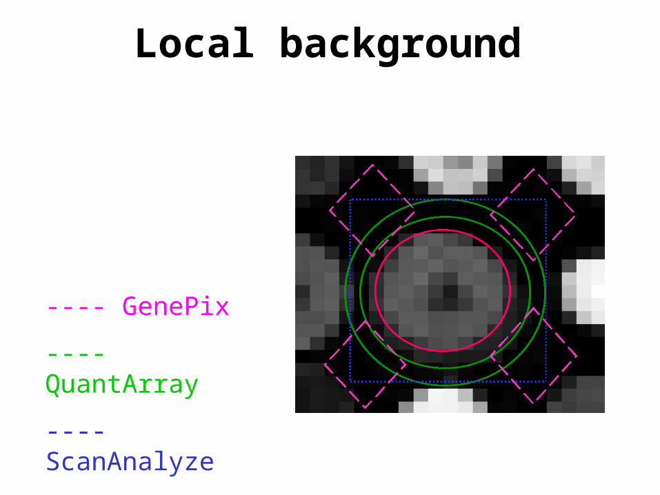
Local background

---- GenePix

---- QuantArray

---- ScanAnalyze

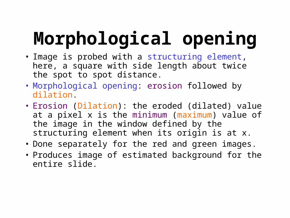
Morphological opening• Image is probed with a structuring element, here, a

square with side length about twice the spot to spot distance.

• Morphological opening: erosion followed by dilation.• Erosion (Dilation): the eroded (dilated) value at a pixel x

is the minimum (maximum) value of the image in the window defined by the structuring element when its origin is at x.

• Done separately for the red and green images.• Produces image of estimated background for the entire

slide.

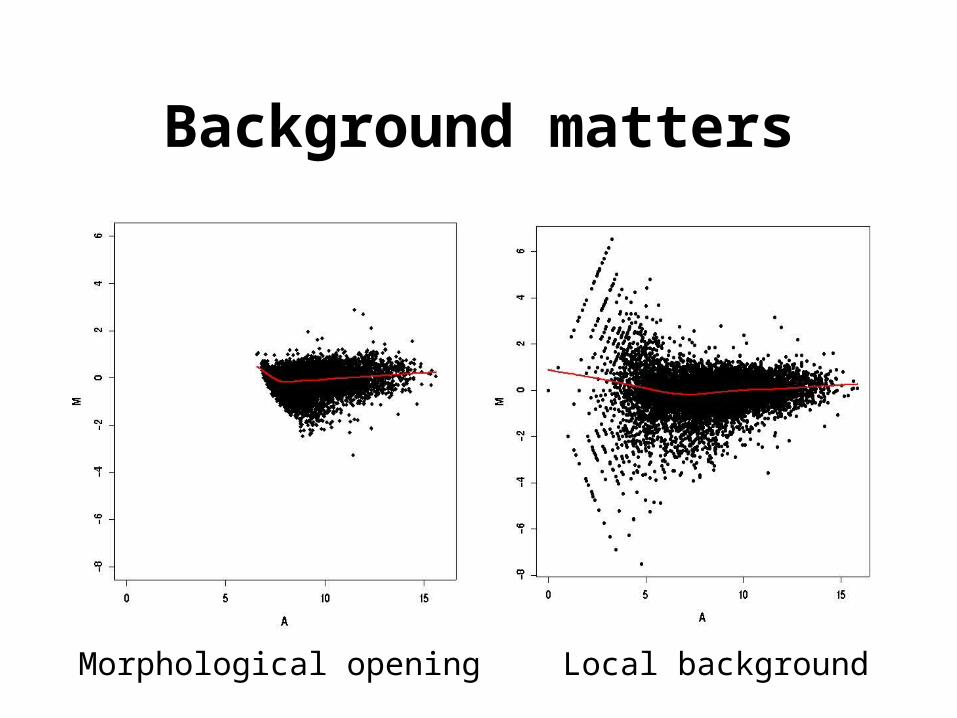
Background matters

Morphological opening Local background

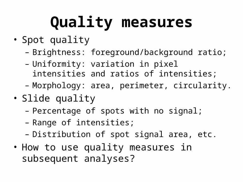
Quality measures• Spot quality

– Brightness: foreground/background ratio;

– Uniformity: variation in pixel intensities and ratios of intensities;

– Morphology: area, perimeter, circularity.

• Slide quality– Percentage of spots with no signal;

– Range of intensities;

– Distribution of spot signal area, etc.

• How to use quality measures in subsequent analyses?

Normalization

Normalization

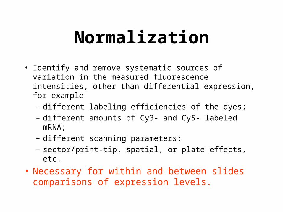
• Identify and remove systematic sources of variation in the measured fluorescence intensities, other than differential expression, for example

– different labeling efficiencies of the dyes;

– different amounts of Cy3- and Cy5- labeled mRNA;

– different scanning parameters;

– sector/print-tip, spatial, or plate effects, etc.

• Necessary for within and between slides comparisons of expression levels.

Normalization

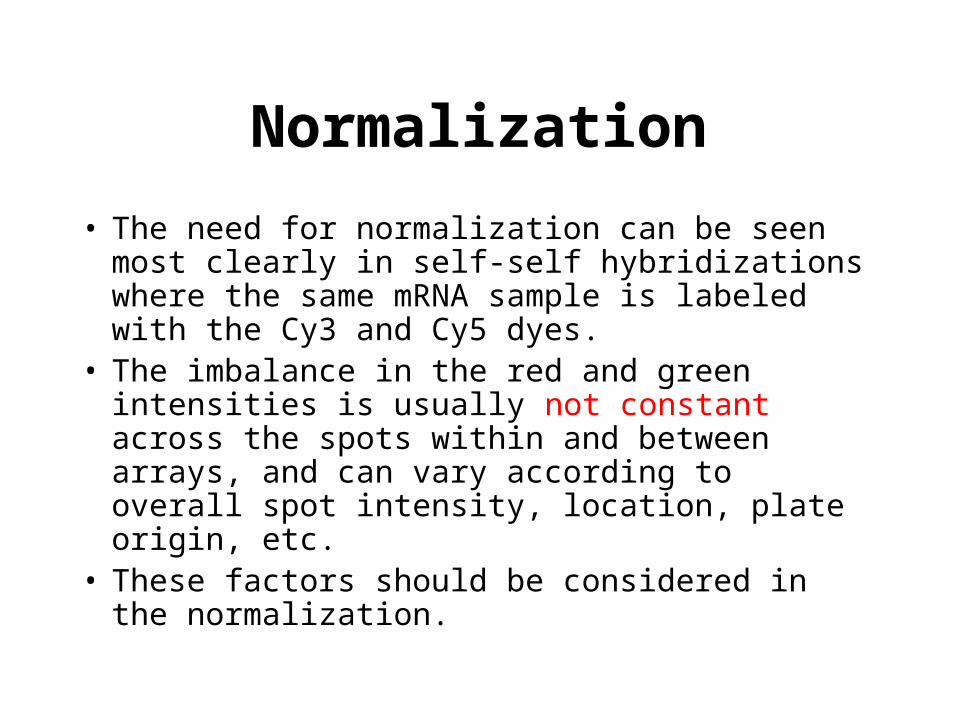
• The need for normalization can be seen most clearly in self-self hybridizations where the same mRNA sample is labeled with the Cy3 and Cy5 dyes.

• The imbalance in the red and green intensities is usually not constant across the spots within and between arrays, and can vary according to overall spot intensity, location, plate origin, etc.

• These factors should be considered in the normalization.

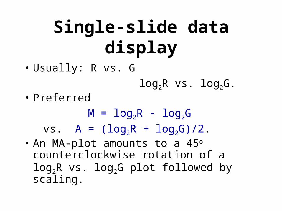
Single-slide data display

• Usually: R vs. G

log2R vs. log2G.• Preferred

M = log2R - log2G

vs. A = (log2R + log2G)/2.• An MA-plot amounts to a 45o

counterclockwise rotation of a log2R vs. log2G plot followed by scaling.

Self-self hybridization

log2 R vs. log2 G M vs. A

Normalization

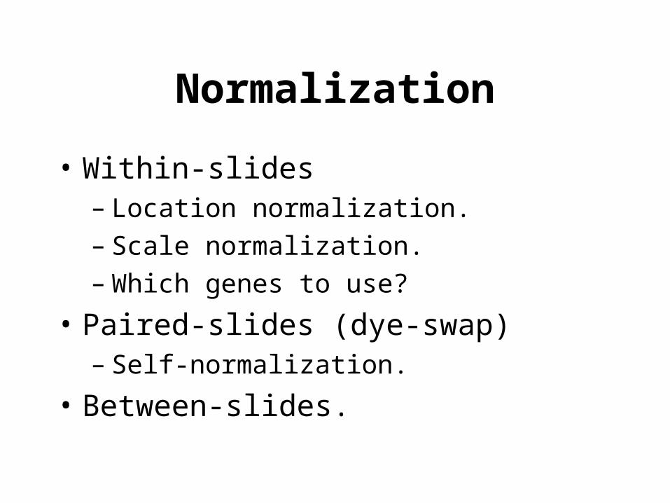
• Within-slides– Location normalization.– Scale normalization.– Which genes to use?

• Paired-slides (dye-swap)– Self-normalization.

• Between-slides.

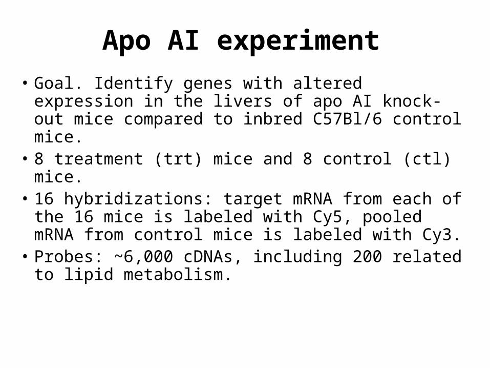
Apo AI experiment

• Goal. Identify genes with altered expression in the livers of apo AI knock-out mice compared to inbred C57Bl/6 control mice.

• 8 treatment (trt) mice and 8 control (ctl) mice.• 16 hybridizations: target mRNA from each of

the 16 mice is labeled with Cy5, pooled mRNA from control mice is labeled with Cy3.

• Probes: ~6,000 cDNAs, including 200 related to lipid metabolism.

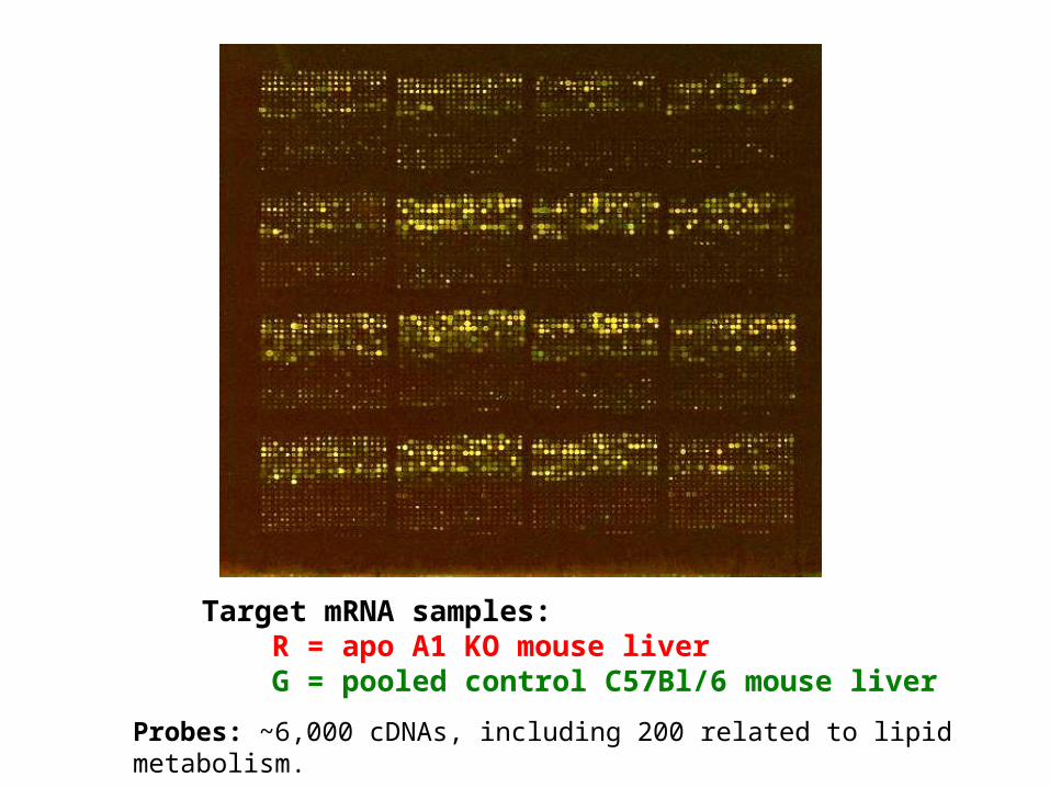
Probes: ~6,000 cDNAs, including 200 related to lipid metabolism.

Target mRNA samples: R = apo A1 KO mouse liver G = pooled control C57Bl/6 mouse liver

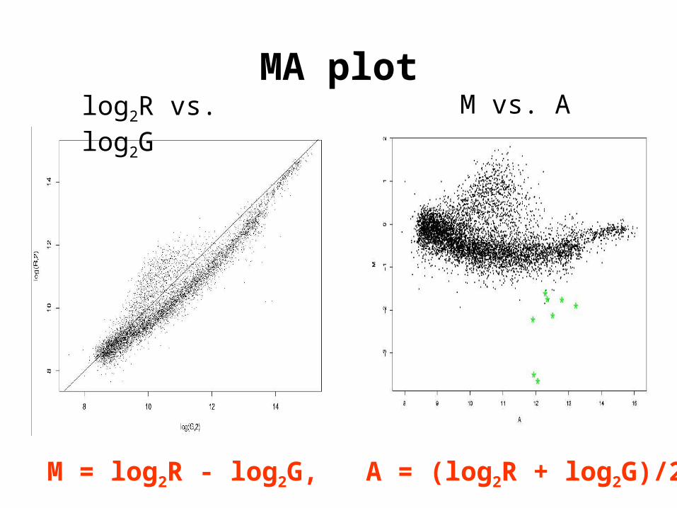
MA plot

M = log2R - log2G, A = (log2R + log2G)/2

log2R vs. log2G M vs. A

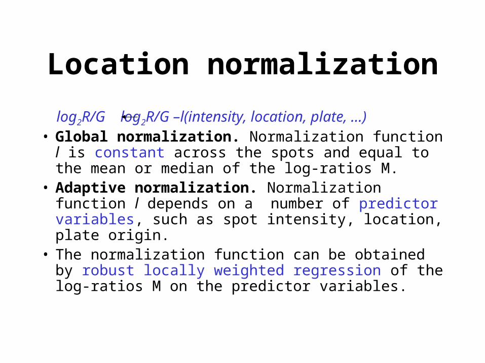
Location normalization

log2R/G log2R/G –l(intensity, location, plate, …)• Global normalization. Normalization function l

is constant across the spots and equal to the mean or median of the log-ratios M.

• Adaptive normalization. Normalization function l depends on a number of predictor variables, such as spot intensity, location, plate origin.

• The normalization function can be obtained by robust locally weighted regression of the log-ratios M on the predictor variables.

Location normalization

• Variable selection.• Many different smoothers are available. E.g. lowess and loess smoothers.• For local regression, choices must be made

regarding: the weight function, the parametric family that is fitted locally, the bandwidth, and the fitting criterion.

• As with any other normalization approach, these choices represent a modeling of the data.

Location normalization

• Intensity dependent normalization. Regression of M on A.

• Intensity and print-tip dependent normalization. Same as above, for each print-tip separately.

• Spatial normalization. Regression of M on 2D-coordinates.

• Other variables: time of printing, plate, etc.

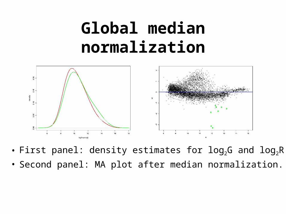
Global median normalization

• First panel: density estimates for log2G and log2R.

• Second panel: MA plot after median normalization.

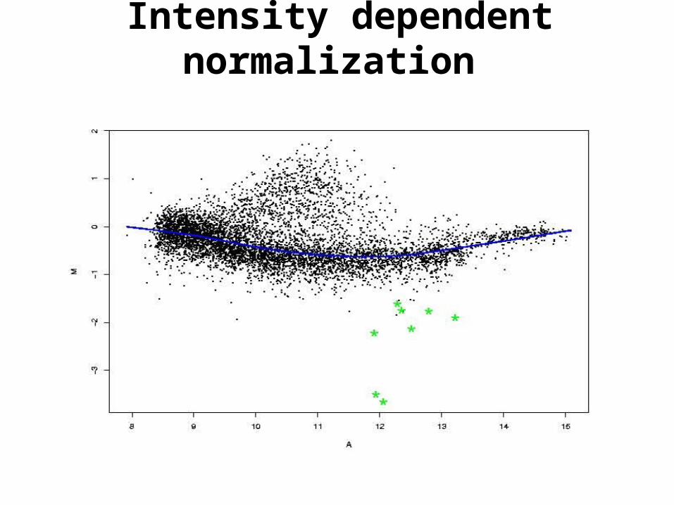
Intensity dependent normalization

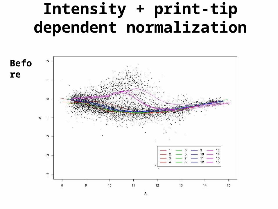
Intensity + print-tip dependent normalization

Before

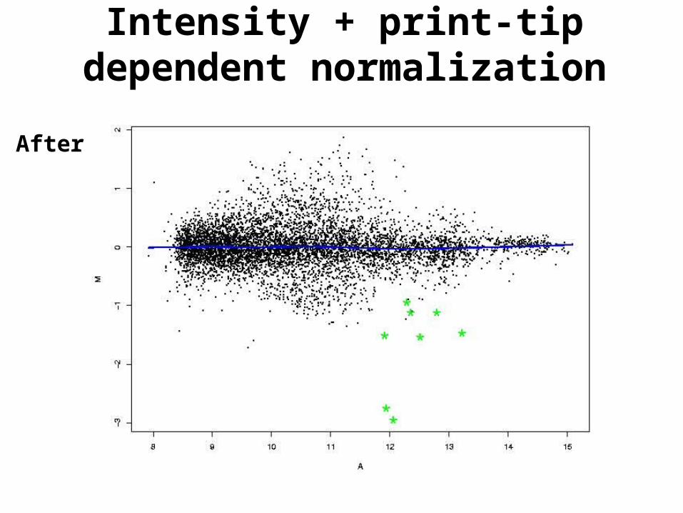
Intensity + print-tip dependent normalization

After

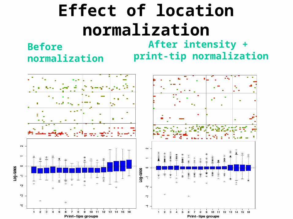
Effect of location normalization

Before normalization After intensity + print-tip normalization

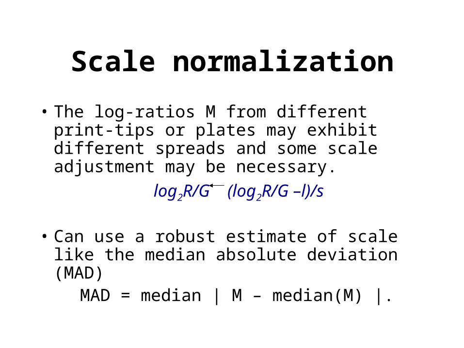
Scale normalization

• The log-ratios M from different print-tips or plates may exhibit different spreads and some scale adjustment may be necessary.

log2R/G (log2R/G –l)/s

• Can use a robust estimate of scale like the median absolute deviation (MAD)

MAD = median | M – median(M) |.

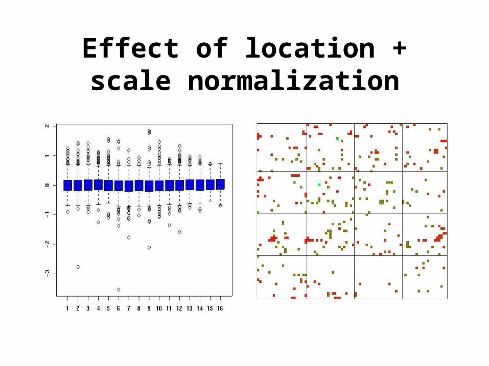
Effect of location + scale normalization

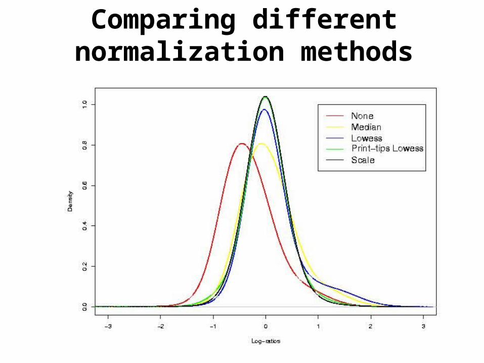
Comparing different normalization methods

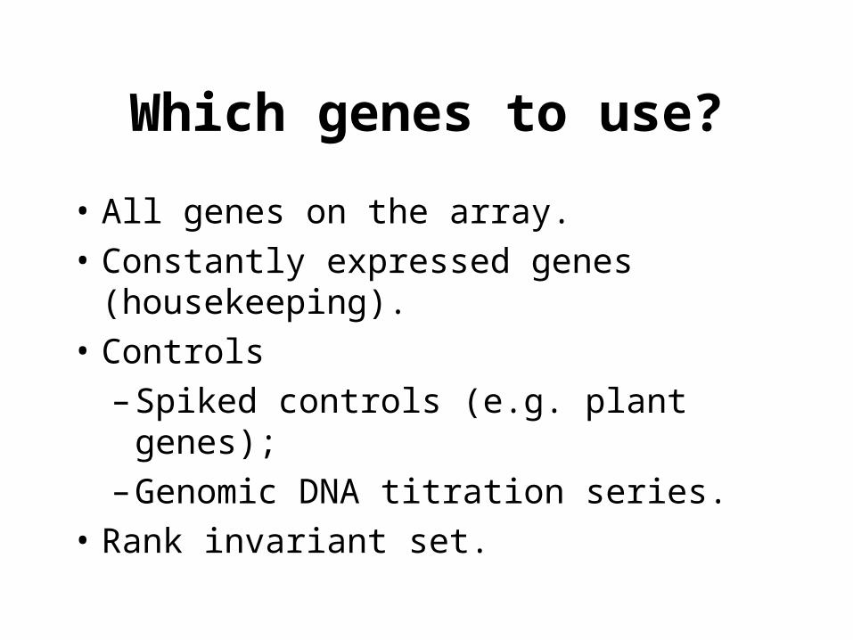
Which genes to use?

• All genes on the array.

• Constantly expressed genes (housekeeping).

• Controls

– Spiked controls (e.g. plant genes);

– Genomic DNA titration series.

• Rank invariant set.

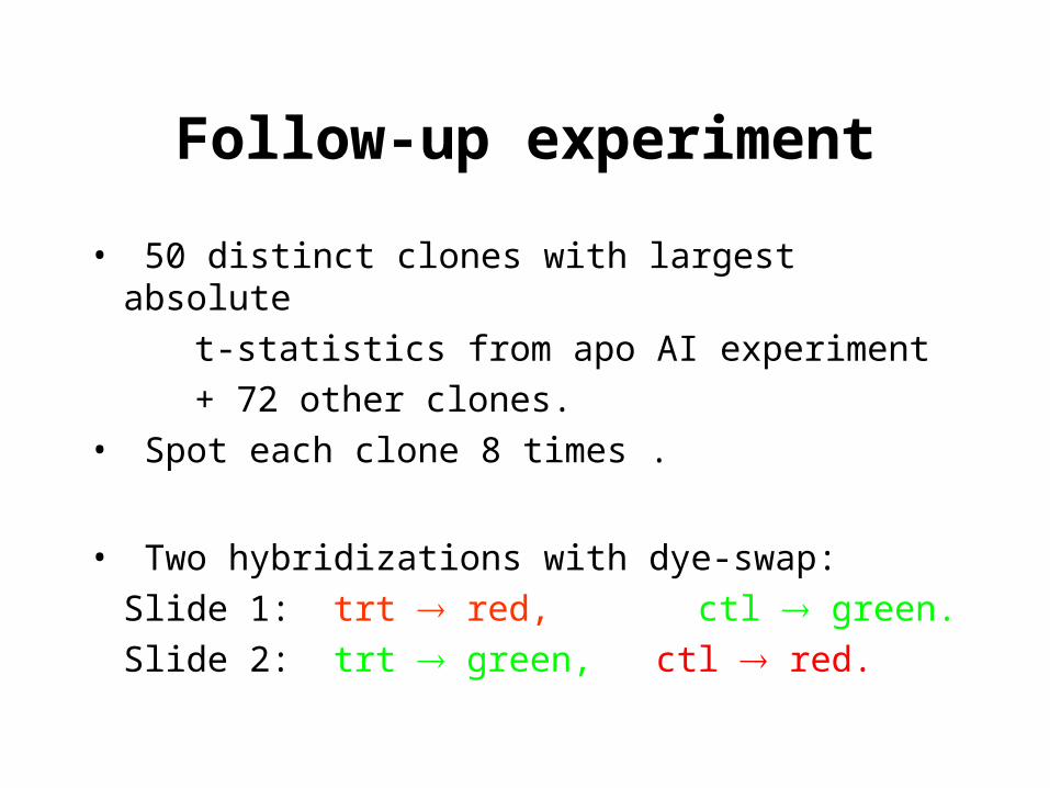
Follow-up experiment

• 50 distinct clones with largest absolute

t-statistics from apo AI experiment

+ 72 other clones.• Spot each clone 8 times .

• Two hybridizations with dye-swap:

Slide 1: trt red, ctl green.

Slide 2: trt green, ctl red.

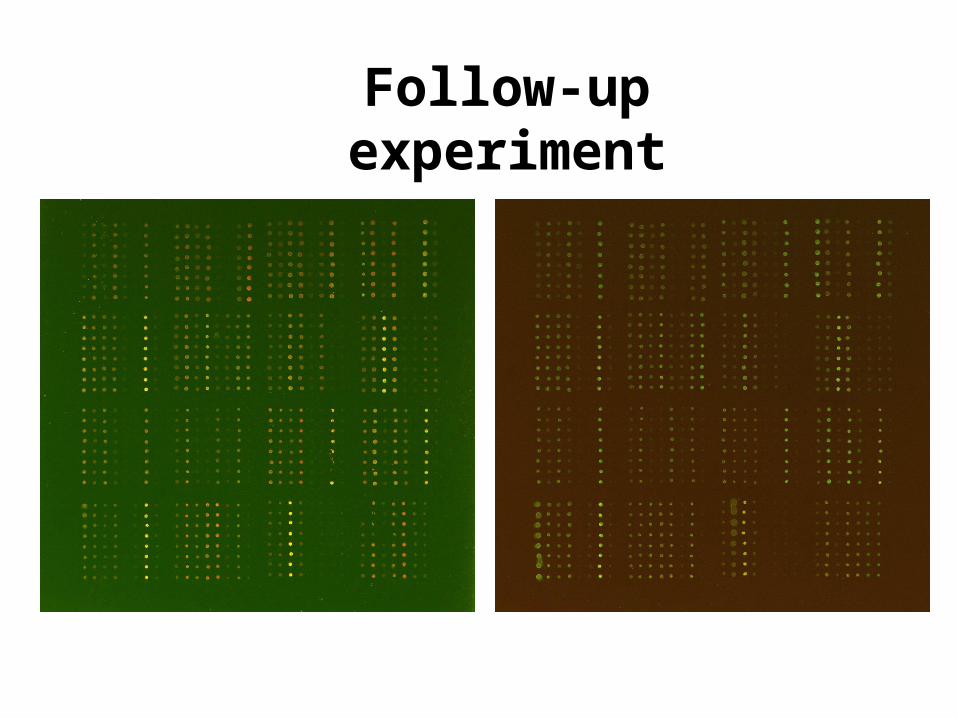
Follow-up experiment

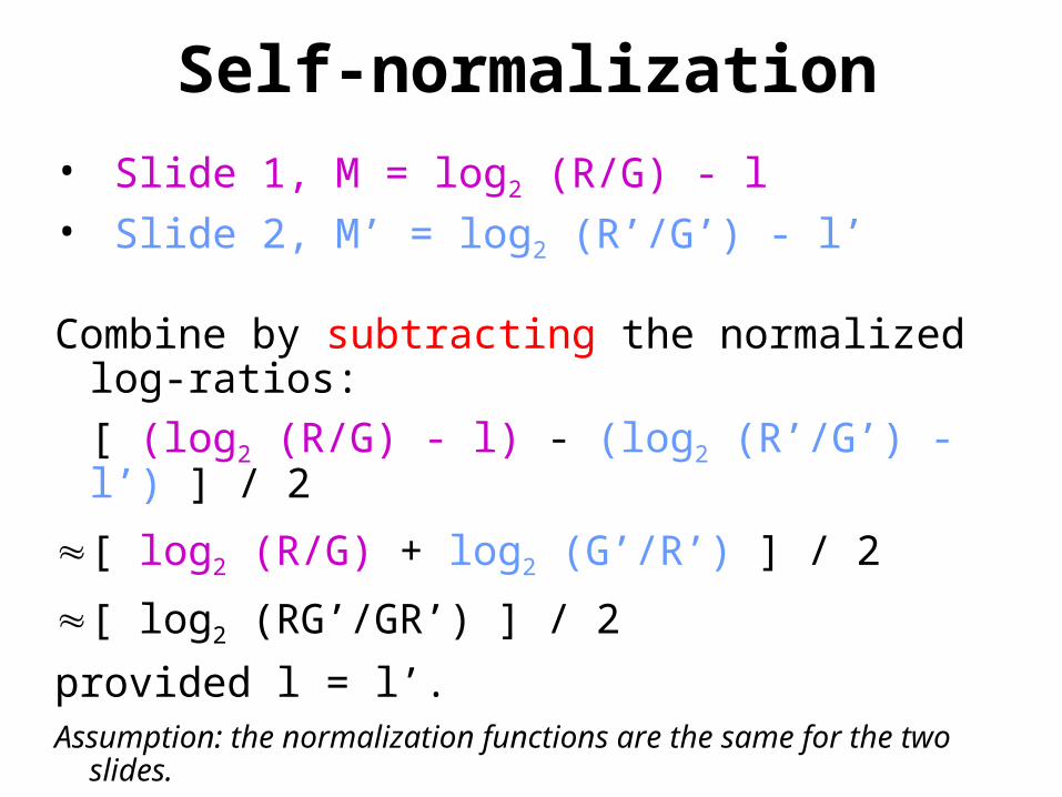
Self-normalization

• Slide 1, M = log2 (R/G) - l• Slide 2, M’ = log2 (R’/G’) - l’

Combine by subtracting the normalized log-ratios:

[ (log2 (R/G) - l) - (log2 (R’/G’) - l’) ] / 2

[ log2 (R/G) + log2 (G’/R’) ] / 2

[ log2 (RG’/GR’) ] / 2

provided l = l’.Assumption: the normalization functions are the same for the two

slides.

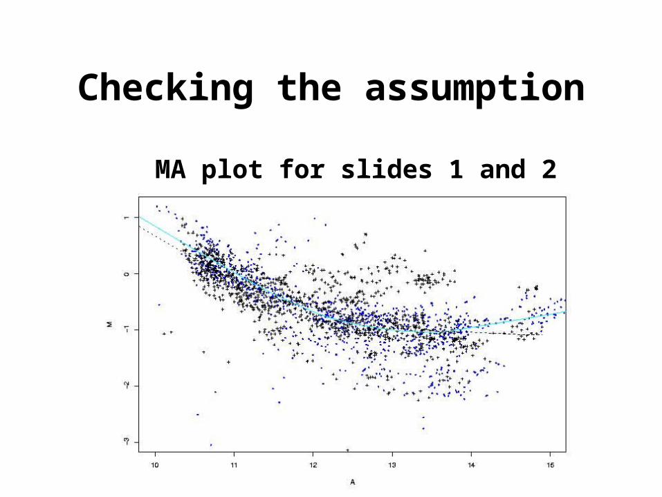
Checking the assumption

MA plot for slides 1 and 2

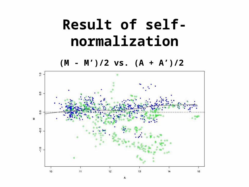
Result of self-normalization

(M - M’)/2 vs. (A + A’)/2

Summary

Case 1. Only a few genes are expected to change.

Within-slides– Location: intensity + print-tip dependent lowess

normalization.– Scale: for each print-tip-group, scale by MAD.

Between-slides– An extension of within-slide scale normalization.

Case 2. Many genes expected to change.– Paired-slides: Self-normalization.– Use of controls or known information.

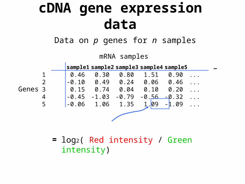
cDNA gene expression data

Genes

mRNA samples

Gene expression level of gene i in mRNA sample j

= log2( Red intensity / Green intensity)

sample1 sample2 sample3 sample4 sample5 …

1 0.46 0.30 0.80 1.51 0.90 ...2 -0.10 0.49 0.24 0.06 0.46 ...3 0.15 0.74 0.04 0.10 0.20 ...4 -0.45 -1.03 -0.79 -0.56 -0.32 ...5 -0.06 1.06 1.35 1.09 -1.09 ...

Data on p genes for n samples

Reading for next Monday

• Robust local regression

W. S. Cleveland. (1979). Robust localy weighted regression and smoothing scatterplots. Journal of the American Statistical Association. 74: 829-836.

• Experimental design

M. K. Kerr & G. A. Churchill. (2001). Experimental Design for Gene Expression Microarrays. Biostatistics. 2: 183-201.