1

Preliminary 2018 Update of the U.S. National Seismic Hazard Model: Overview of Model, Changes, and Implications

M.D. Petersen, A.M. Shumway, P.M. Powers, C.S. Mueller, M.P. Moschetti, A.D. Frankel, S.

Rezaeian, D.E. McNamara, S.M. Hoover, N. Luco, O.S. Boyd, K.S. Rukstales, K.S. Jaiswal, E.M. Thompson, B. Clayton, E.H. Field, and Y. Zeng

We value and seek the feedback of the public and informed technical community on the 2018 Update of the U.S. National Seismic Hazard Model. This draft manuscript is only shared for

purposes of scientific peer review and public feedback. Because the manuscript has not yet been approved for publication by the U.S. Geological Survey (USGS), it does not represent any official

USGS finding or policy and should not be used in any engineering or other application at this time. The draft will be available on our website (https://earthquake.usgs.gov/hazards/) from

November 7, 2018 to December 7, 2018 for public comment.

Abstract During 2017-2018, the National Seismic Hazard Model (NSHM) was updated by incorporating (1) new median ground motion models, new estimates of their epistemic uncertainties and aleatory variabilities, and new soil amplification factors for the central and eastern U.S., (2) amplification of long-period ground motions in deep sedimentary basins in the Los Angeles, San Francisco, Seattle, and Salt Lake City areas, (3) an updated seismicity catalog, which includes new earthquakes that occurred between 2012 and 2017, and (4) an improved computer code and implementation details. Results show increased ground shaking in many (but not all) locations across the central and eastern U.S., as well as near the four aforementioned urban areas in the western U.S. More people live or work in areas of high or moderate seismic hazard than ever before, leading to higher risk of undesirable consequences from future ground shaking.

Introduction Over the past four decades, the U.S. National Seismic Hazard Model (NSHM) Project of the U.S. Geological Survey (USGS; e.g., Algermissen and Perkins, 1976; Frankel et al., 1996, 2002b; Petersen et al., 1996, 2008, 2014, 2015) has provided science-based hazard information for use in seismic provisions of U.S. building codes for buildings, bridges, railways, and defense facilities (e.g., from NEHRP, ASCE, IBC, AASHTO, AREMA, UFC)1, among other structures; risk assessments for insurance and disaster management planning (e.g., Core-logic, AIR, RMS)2; and federal, state, and local governmental policy decisions (e.g., U.S. Army Corps of Engineers, Bureau of Reclamation, FEMA, California Geological Survey, local land use plans)3. These probabilistic seismic hazard models integrate two fundamental inputs (Cornell, 1968): (1) earthquake rupture forecast models, which define a potential range of earthquakes that could strike at any location across the U.S. and (2) ground motion models (GMMs), which provide estimates of the potential range of ground shaking from each event. Seismic hazard forecasts from such models show where

1 National Earthquake Hazard Reduction Program (NEHRP), American Society of Civil Engineers (ASCE), International Building Code (IBC), American Association of State Highway and Transportation Officials (AASHTO), American Railway Engineering and Maintenance-of-Way Association (AREMA), Unified Facilities Criteria (UFC). 2 Core-logic Catastrophe Risk Management (Core-logic), Air Worldwide (AIR), Risk Management Solutions (RMS). 3 Federal Emergency Management Agency (FEMA).

2

and how often future earthquake ground shaking might occur. Probabilistic seismic hazard forecasts can be employed to encourage safer building designs in areas with high shaking potential while saving resources in areas with lower shaking hazard. This information, coupled with various prudent mitigation strategies, can facilitate resilient communities that can function better following an earthquake-related disaster. Figure 1 shows an example 2018 chance of damage map for 100 years (M5+ earthquakes) that includes population density. The population density comes from the Landscan with 1 km x 1 km resolution (Dobson et al., 2000). The 2018 NSHM is based on the best science, data, models, and methods available at the time of this publication, with information obtained through an open request for hazard modeling contributions, a NSHM workshop, and interactions with hundreds of partners and technical experts across the country. Collaborators provide technical advice, review model details, and include: (1) nine members of the NSHM Steering Committee who serve as active participatory experts in the development and review of the model4; (2) other technical experts from USGS and other federal, state, and local government agencies as well as from academia and industry; and (3) those who attended our public 2018 NSHM workshop and submitted comments during our review period5. Many scientists and organizations (e.g., PEER and SCEC)6 contributed to development of the local velocity models, earthquake catalog, seismicity models, GMMs, standard deviation (sigma) models, and soil amplification models. Ground shaking hazard maps, models, and subsidiary products can be incorporated into many practical applications for mitigating earthquake risk. However, their usefulness depends on continuing interactions with end-users, particularly during the product development stages. Engineers are a major end-user of the NSHMs, and they also provide requests to USGS on the types of hazard products needed for building codes. For example, the Building Seismic Safety Council (BSSC) Provisions Update Committee and Project ‘17 are FEMA-sponsored engineering efforts whose objective is to improve building code procedures by meshing the best available science information and sound engineering principles, in collaboration with the USGS. In past and current versions of their provisions, the BSSC enacted design procedures (e.g., Luco et al., 2015) that required hazard estimates for peak horizontal ground acceleration (PGA) as well as 0.2 second (s) and 1s spectral accelerations (SA) with a firm-rock site condition of 760 m/s VS30 (time-averaged shear wave velocity in the upper 30 meters, m, of the crust). These ground motion values parameterize simplified response spectral shapes that can be used in designing earthquake-resistant buildings and other structures. Past versions of the NSHMs focused on the three oscillator periods and the firm-rock site class; although additional periods and site class maps were also developed (e.g., Shumway et al., 2018) which were not used in previous building codes. With the additional ground shaking information that recently became available for the central and eastern U.S. (CEUS) through the release of the Next Generation Attenuation Relationships for the Central and Eastern North America Region (NGA-East) and corresponding site amplification factors (Stewart et al., 2017 and Hashash et al., 2017), BSSC’s Project ‘17 requested that USGS produce a new series of hazard

4 John Anderson (chair), Yousef Bozorgnia, Kenneth Campbell, Martin Chapman, C.B. Crouse, Heather DeShon, Tom Jordan, Nilesh Shome, and Ray Weldon. 5 Open review period began in March 2018 at workshop but extends to the end of November with about a month review of the documentation. 6 Pacific Engineering Research Center (PEER), Southern California Earthquake Center (SCEC).

3

values for directly assessing the design ground motions at additional periods and site classes (i.e., multi-period response spectra, BSSC website: https://www.nibs.org/page/bssc_P17C). These more detailed products serve to improve the building code design procedures. Thus, the 2018 NSHM accounts for many more oscillator periods and site classes across the conterminous U.S. than have been available in previous NSHMs. Ground motion observations (e.g., Field. 1996; Frankel et al., 2002a; Pratt et al., 2003; Graves et al, 2011; Frankel et al., 2009; Chang et al., 2014; Frankel et al., 2018) and 3D simulations (e.g., Aagaard et al., 2008; Graves et al, 2011; Roten et al., 2011; Moschetti et al., 2017; Frankel et al., 2018; Wirth et al., 2018b) indicate that deep sedimentary basins strongly amplify long-period (≥ 1 s) ground motions. The ground-motion models used in the NSHMs to date did not include this deep-basin amplification. While some of the strong-motion recordings used to develop the crustal earthquake GMM’s are located on basins, the average (default) basin depth is only 1-3 km in the Campbell and Bozorgnia (2014) GMM, as measured by Z2.5, the depth to a Vs of 2.5 km/s. Thus, the observed amplification of the Seattle basin, which has a maximum Z2.5 of 7 km (Stephenson et al., 2017) is not accounted for in the current NSHMs. This is also true for the deeper portions of the Los Angeles and Ventura basins in southern California, the Livermore and other basins in the San Francisco Bay area, and a limited portion of the Salt Lake City basin (see below). Other NGA West GMM’s use Z1.0 the depth to a Vs of 1.0 km/s to characterize basin depth. Again, the default basin depths used in the GMMs for a given Vs30 are much smaller than the maximum depths of the aforementioned basins. For this update we are considering for the first time basin depth factors that modify the long-period shaking in four urban areas. In addition to building code developers, there are many other important end-users of the NSHMs, such as insurance industry, risk modelers, and policy makers. The insurance industry typically applies risk models generated by third-party risk modeling corporations who apply information from the NSHMs that are needed for estimating the ground shaking peril and its catastrophic losses. Public policy makers use the models to address disaster mitigation priorities. An example of how these maps are applied in public policy is illustrated through the tools provided by FEMA, which incorporate the USGS hazard models directly in their computer programs to assess earthquake risk to the nation and help communities prepare for earthquake shaking (e.g., FEMA 366 and HAZUS software; Jaiswal et al., 2015, 2017; http://www.fema.gov/hazus/). Other examples of end-users are the U.S. Army Corp of Engineers and Bureau of Reclamation who use the models in assessing earthquake risk for dams and other important facilities. The NSHMs can be useful for prioritizing retrofit schedules, reassessing vulnerable structures, or developing risk mitigation strategies. An updated assessment of the population that is exposed at alternative risk levels is considered in this publication. In this paper, we provide an overview of the 2018 NSHM update for the conterminous U.S., comparisons with the 2014 NSHM, final products, and some implications of the model on seismic risk. When comparing the 2018 NSHM with the 2014 NSHM, we are using the most recent set of maps calculated for the 2014 NSHM (which includes additional periods and site classes, as explained below; Shumway et al., 2018). We also describe the following published information that was submitted before March 2017 and discussed at our 2018 NSHM Update workshop: (1) new earthquake catalogs and forecasts that account for locations of future earthquakes, (2) models for assessing multiple periods and site-amplified ground shaking for sites across the CEUS, (3) basin

4

shaking amplification models for long-periods across urban areas in California, Washington, and Utah, and (4) other computer code and modeling details. In addition to describing inputs and modeling assumptions, we examine the results of the 2018 NSHM and deconstruct the hazard to ascertain which inputs and assumptions contribute most to the changes in hazard. The changes are mostly caused by (1) modifications to the earthquake catalog and smoothed rate grids, (2) new CEUS GMMs, and (3) basin amplification effects caused by new data from seismic velocity models with the factors included in selected WUS GMMs. The USGS NSHMs have been updated every six years to incorporate the new data, models, and methods that improve the hazard forecasts. This 2018 update, however, is being issued just four years following its 2014 predecessor, to provide additional time for the building code community to evaluate the new hazard models and their impacts. The new models will be considered for incorporation in the 2020 NEHRP Provisions, 2022 ASCE7 Standard, and the 2024 IBC, as well as other building code, risk, and policy implementations.

2018 NSHM Workshop On March 7-8, 2018, the National Seismic Hazard Model Project (NSHMP) held a public workshop in Newark, California to discuss new hazard information for updating the NSHM and to build community consensus on the best methods, data, and models to apply in the assessment. This workshop was attended in-person and on-line by about 140 science and engineering experts across the country, and resulted in the following six recommendations:

(1) For the CEUS, workshop participants expressed strong support for considering the new NGA-East for USGS GMMs (Goulet et al., 2017) and the new soil amplification factors for the CEUS (Stewart et al., 2017; Hashash et al., 2017). However, concern was expressed that the 13 interim NGA-East for USGS GMMs were similar to a backbone type model7. Backbone curves do not allow for significant differences in shapes of the median curves, lack the details expressed in some of the underlying physics-based models, and do not encompass alternative ground motion correlations with distance or magnitude (Goulet et al., 2017). One important objective of the NGA-East project was to get away from backbone-type models and allow for a fuller depiction of the epistemic uncertainty. Participants at the workshop suggested that USGS compare the 13 NGA-East for USGS GMMs available during the workshop with an updated set of 17 NGA-East for USGS GMMs. (2) For the CEUS, participants also expressed support for including the original Seed GMMs (PEER, 2015) that were used in the Sammon’s mapping process (Goulet et al., 2017) to develop the NGA-East for USGS GMMs, as well as several updated Seed GMMs (Graizer, 2016; Graizer, 2017; Shahjouei and Pezeshk, 2016) that were developed after publication of the NGA-East for USGS GMMs. We only considered the Seed GMMs that met the selection criteria established for this update. Some of the workshop participants indicated that independent analysis by different modeling groups would allow for broader epistemic uncertainty and more physics-based variability and correlations in the models.

7 Backbone models assume that a median model can be scaled up or down to encompass the center, body, and range of the potential ground motions (Goulet et al., 2017).

5

(3) For the CEUS, participants supported adding additional aleatory variability to account for site-to-site variability (𝝓S2S) in the model. (4) For the CEUS Gulf Coast, participants recommended that USGS not incorporate Gulf Coast regional ground shaking adjustments in the 2018 NSHM update due to time constraints but encouraged their considerations in future updates. (5) For the WUS, participants supported the proposal to include basin amplification terms for long periods across the four urban areas for which published local velocity models are available. However, attendees had mixed opinions on whether or not to allow the basin terms to deamplify the GMMs relative to the default basin depths for a given VS30. Concerns were raised about the accuracy of the local 3D velocity models, the ability of the basin terms in the GMMs to model basin effects, and how to avoid abrupt offsets outside of the urban regions. (6) For the conterminous U.S., participants encouraged preparation of an updated earthquake catalog and improved computer code resources.

We considered the recommendations from participants at the workshop to develop the final 2018 NSHM update.

Update of Earthquake Catalog and Rate Models

For this 2018 NSHM, we developed new seismicity catalogs for the CEUS and WUS that were updated through 2017 to account for earthquakes that occurred since the last model was constructed. Gridded, smoothed seismicity-based models account for potential earthquakes that do not occur on modeled faults. In this section, we describe the earthquake catalog development, the gridded (smoothed) seismicity model, and present the 2018 seismicity-based model along with comparisons to the 2014 NSHM. Earthquake Catalog Development A critical component of the NSHMs is an earthquake catalog that can be used to assess the sizes and locations of past earthquakes and guide us in our assessment of where and how often future earthquakes might take place. The catalog used for the 2014 NSHM ended in 2012. To update the catalogs for both the CEUS and WUS through 2017, we incorporated new data from the USGS, the Geological Survey of Canada, and Saint Louis University. We used the methodology described by Mueller (2018) to develop catalogs that are suitable for seismic hazard analysis: converting original magnitudes to uniform moment magnitudes (Mw), deleting duplicate events, deleting non-tectonic events, and declustering. Mueller (2018, figure 2) shows the polygons that are used to exclude induced earthquakes in the CEUS. For the time spans used to exclude induced earthquakes, see Petersen et al. (2016a, table 1). In several cases, such as Oklahoma-southern Kansas and north-central Arkansas, the polygon boundaries used for the 2018 NSHM have been updated from 2014. As shown by Petersen et al. (2016a), new zones have been added (for example, near Alice, Texas, and Perry, Ohio). The catalog and earthquake sources for California are not updated for the 2018 NSHM. The California earthquake rates are interwoven into the UCERF3 model which will be updated when new source models are available (Field et al., 2014).

6

There are several challenges in developing the NSHM catalogs and seismicity-based statistical models that rely on an independent set of tectonic earthquakes. One important challenge is to consistently and uniformly estimate Mw for small earthquakes and for some older earthquakes. As discussed below, one possible way to lessen the impact of these uncertainties would be to raise the magnitude threshold for the seismicity recurrence analysis, for example, from M2.7 to M3.0. In the future, more refined classifications of the data by source catalog, era, or region might also lead to improved procedures for estimating Mw and for identifying duplicates. Another important challenge lies in developing declustered models that remove the dependent earthquakes such as foreshocks and aftershocks, leaving an independent set of earthquakes that can be used in the hazard assessment. Declustering is a topic of active research since clusters of earthquakes may exhibit regional statistical characteristics. The NSHM catalogs are declustered using the methodology of Gardner and Knopoff (1974), which is based on California data. Analyses of various declustering methods suggest that this method of declustering is reasonable for tectonic earthquakes across the U.S. (e.g., CEUS-SSCn, 2012). However, recent results for induced earthquakes in Oklahoma indicate possible declustering problems there, at least for the largest events (Petersen et al., 2016a, 2016b, 2017, 2018). A third challenge is to identify explosions and mining-related seismic events using the limited available information. Gridded or Smoothed Seismicity-Based Rate Models New gridded, smoothed earthquake rate forecasts were developed for the CEUS and WUS (outside of California) using the updated catalogs, assuming that future earthquakes will occur near the locations of past events. Accounting for catalog completeness, earthquakes are counted and rates (10a values) are computed on a 0.1°-latitude-by-0.1°-longitude grid for each region. Completeness varies by region, reflecting patterns of written history and seismic network coverage. The models assume that earthquakes follow exponential magnitude-frequency distributions. Regional b-values used in the analysis are unchanged from the 2014 NSHM: 1.0 for the CEUS and 0.8 for the WUS. To smooth the gridded rates, we apply fixed-kernel and adaptive-kernel (nearest-neighbor) smoothing methods (Frankel, 1995; Petersen et al., 2014; Moschetti et al., 2015). As in the 2014 logic tree, the fixed-kernel model is assigned 0.6 weight and the adaptive-kernel model 0.4 weight. Parameters such as minimum magnitudes of completeness, b-values, and smoothing distances differ for the fixed- and adaptive-smoothing models. The two models represent an important epistemic uncertainty in the NSHM source model (Moschetti et al., 2015). Both models consider statistical based counts of earthquakes in a particular grid cell (10a values). The 2014 version of the UCERF38 smoothed seismicity model (Field et al., 2014) is used for California, so the seismicity rate forecasts have not changed for the 2018 update. The fixed-kernel smoothing applies a two-dimensional Gaussian operator with 50 km or 75 km correlation length (Frankel, 1995). This model uses a fixed value to assess reasonable distances between future and past earthquakes. The WUS completeness model is unchanged from previous NSHMs: M4+ since 1933, M5+ since 1900, and M6+ since 1850 for a zone encompassing the seismically active parts of coastal and central California, and M4+ since 1963, M5+ since 1930, and M6+ since 1850 for the rest of the WUS. The CEUS completeness zonation is modified in two ways from the 2014 NSHM, which was, in turn, roughly based on (CEUS-SSCn, 2012): (1) The zone

8 UCERF, Uniform California Earthquake Rupture Forecast.

7

encompassing the Washington–New York–Boston corridor is extended southwestward into central Virginia and (2) The westernmost zone is divided at -100° longitude and extended westward to the NSHM CEUS boundary; -100° is used because it corresponds to a change in the MD,ML-to-Mw conversion formulas (CEUS-SSCn, 2012). We determine completeness years for magnitudes 2.7+, 3.7+, and 4.7+ for each of the seven completeness zones by examining numbers of earthquakes in magnitude and time bins; results are similar to the 2014 NSHM. Figure 2 shows the 2018 CEUS earthquake catalog and completeness zonation that we apply for the fixed-kernel smoothing model. The adaptive-kernel smoothing employs smoothing distances, based on a nearest-neighbor parameter (Helmstetter et al., 2007), that have the effect of spatially concentrating seismicity rates in regions of high seismicity and of diffusing seismicity rates in regions of low seismicity, relative to fixed-kernel smoothing. The method uses event-specific smoothing distances that are identified by optimizing a joint log-likelihood parameter (Helmstetter et al., 2007; Werner et al., 2011; Moschetti, 2015). Application of the adaptive smoothed seismicity method to the WUS and CEUS employed separate earthquake catalogs and likelihood testing to identify smoothing parameters. Likelihood-derived smoothing parameters were not updated for the 2018 NSHM from what was applied in the 2014 NSHM. Because extending the duration of the earthquake catalog increases the number of earthquakes, use of a constant neighbor-smoothing-number for increasing catalog durations will have the overall effect of spatially concentrating seismicity rates. To counteract this effect, we hold the neighbor-number and catalog durations constant by shifting the catalog start times by the five years added to the end of the catalog when it was updated. For the adaptive model in the WUS, a neighbor-number of three was identified in previous likelihood testing (Petersen et al., 2014, 2015) while a neighbor-number of four was identified from likelihood testing for the CEUS region (Moschetti, 2015). For the 2018 update of the adaptive-kernel model, we applied the following input parameters and data. The WUS smoothed seismicity model used the updated, declustered WUS earthquake catalog. Minimum magnitude of completeness was M=4, since 1963, with a b-value of 0.8 applied across the entire region. The CEUS adaptive smoothed seismicity model used the updated, declustered CEUS earthquake catalog. The minimum magnitude of completeness was M=3.2 in the adaptive model, with spatially variable completeness times defined using the zones described by Petersen et al. (2014) and completeness values computed by Moschetti (2015). A comparison of final weighted models developed in 2018 and 2014 are shown in Figure 3. The changes in adaptively smoothed earthquake rates result from the smaller smoothing distances in regions of higher seismicity and larger smoothing distances in regions of diffuse seismicity, compared to the fixed smoothing results. In most places, differences in the forecast earthquake rates between the two smoothing models are not large and do not result in significant changes to hazard. As mentioned above, we have tested the sensitivity of the seismic hazard to raising the magnitude threshold (Mmin) in the seismicity recurrence calculation from Mmin=2.7 to Mmin=3.0 in the CEUS. The result was sensitive to single earthquakes in areas of sparse seismicity and not very robust. The largest changes caused by applying the Mmin=3.0 model result in decreased hazard over small areas of the New Madrid and the eastern Tennessee seismic zones. Pending further research, we have not applied this alternative in the 2018 update.

8

Hazard Changes Caused by New Smoothed Seismicity Models Figure 4 shows a comparison of the 2014 and 2018 seismicity-based hazard forecasts for 0.2s SA at 2% probability of exceedance in 50 years. Increases in ground shaking generally occur near new areas of heightened activity: near Delaware, southern Ohio and northern West Virginia, Kansas, Alabama, Nevada, and New Mexico. Increased hazard in Oklahoma, Kansas, Ohio, Texas, Arkansas, and Alabama are most likely associated with remaining induced earthquake activity that was not removed during the declustering process (Petersen et al., 2016a, 2016b, 2017, 2018). Higher hazard also occurred near the New Madrid Seismic Zone (NMSZ) where seismicity has increased over the past few years (Petersen et al., 2016a, 2016b, 2017, 2018). Hazard has decreased in parts of Utah, Wyoming, and Colorado, probably due to a modification in the procedure for computing Mw there. Ratios in these states indicate the new models are generally lower by about 20% with differences less than 0.1g compared to the 2014 models. Seismic hazard changes caused by the updated earthquake catalog are quite minimal because they mostly reflect the incremental changes to the rate of earthquakes. They are more pronounced increases in places where new earthquakes have occurred during the past hundred years.

Update of Ground Motion Models in the Central and Eastern U.S.

The 2018 NSHM incorporates new ground shaking information that was not previously available for the CEUS (Rezaeian et al., 2015). We use new GMMs developed by the NGA-East Project (Goulet et al., 2017), new estimates of aleatory variability (sigma; Appendix A), and new estimates of site amplification factors (Appendix B). These models result in significant changes to ground shaking hazard. CEUS Median Ground Motion Models and Weights The NGA-East Project developed two new sets of GMMs: (1) 19 adjusted Seed GMMs that are developed by independent modelers using a standardized set of data and simulations (PEER, 2015) and (2) 17 updated “NGA-East for USGS” GMMs developed by an integrator team that better account for epistemic uncertainty in the mean ground motions as a function of magnitude, distance, and oscillator period. The adjusted Seed GMMs were developed by independent modelers using their interpretations of the best data and science available. Two of the Seed GMMs were subsequently updated to account for new information and enhanced modeling techniques: Graizer (2016) and an alternative Graizer (2017), and Shahjouei and Pezeshk et al. (2016). Based on recommendations from the NGA-East Project, our GMM selection criteria, and considering updates from modelers to their Seed GMMs, we reduced the number of Seed GMMs from 19 models to 14 models, which we refer to as the Updated Seed GMMs. We originally considered 13 interim NGA-East for USGS GMMs (McNamara et al., 2018) that developers recommended to USGS, but the developers later added an addendum to their report recommending that USGS apply the 17 updated NGA-East for USGS GMMs, which better account for epistemic uncertainty and correlations between models and are more similar to the final NGA-East models (Goulet et al., 2017; with 2018 addendum). The new CEUS GMMs used in the 2018 NSHM are based on the two sets of GMMs (Updated Seed GMMs and NGA-East for USGS GMMs) and on a site condition characterized by 3,000 m/s VS30 and kappa of 0.006 seconds, magnitudes from M4 to 8, distances out to 1,000 km, and median (RotD50) spectral accelerations with 5% damping for periods from 0.01 to 10 seconds. Logic tree

9

weights assigned to the Updated Seed GMMs are based on the 2014 NSHM methodology that considers grouping of GMMs based on their model types and geometric spreading features, as well as some judgement on our confidence in their performance based on extrapolations and available residual analysis (Table 1; Rezaeian et al., 2015). Weights for the NGA-East for USGS GMMs are provided by the NGA-East modeling teams and are based on Sammon’s mapping methodology. Overall the Updated Seed GMMs receive ⅓ (0.333) weight to account for alternative models that are developed by independent modelers and the NGA-East for USGS GMMs receive the other ⅔ (0.667) weight to account for the additional effort by the developers to quantify the epistemic uncertainty more fully, as discussed at the 2018 NSHM Update workshop (Fig. 5). The new 2018 NSHM CEUS GMMs represent a significant advancement in the forecasting of ground shaking in the CEUS for many new periods and site classes and based on new strong motion data and simulations. Table 1: Updated Seed GMMs Logic Tree

Geometric Spreading (< 50-70 km) Model Type Model Model Weight R-1 (0.33) Point Source (0.67) B_BCA10D (0.3) 0.06633

B_AB95 (0.1) 0.02211

B_BS11 (0.1) 0.02211

2CCSP (0.25) 0.055275

2CVSP (0.25) 0.055275

Traditional Empirical2 (0.33)

Graizer163 (0.5) 0.05445

Graizer174 (0.5) 0.05445

R-1.3 (0.33) Hybrid Empirical (0.33) PZCT15_M1SS (0.5) 0.05445

PZCT15_M2ES (0.5) 0.05445

Hybrid Empirical and Broadband (0.33)

SP165 (1.0) 0.1089

Stochastic Equivalent Point Source (0.34)

YA15 (1.0) 0.1122

Other1 (0.34) Other (1.0) HA156 (0.33) 0.1122

Frankel157 (0.33) 0.1122

PEER_GP7 (0.34) 0.1156

1 Geometric spreading different from R-1 or R-1.3. 2 Spectral shapes developed for the WUS empirically adjusted to CEUS. 3 Graizer16 is an update of the NGA-East Seed model Graizer15. 4 Graizer17 is an alternative to the Graizer16 model.

10

5 SP16 is an update of the NGA-East Seed model SP15. 6 Reference Empirical. 7 Simulation-based Hybrid. Figures 6 and 7 show the weighted means for each set of GMMs considered in the 2014 and 2018 update as a function of distance and oscillator period, respectively. The new NGA-East for USGS and Updated Seed averaged GMMs are very similar to the averaged value of the group of GMMs applied in the 2014 NSHM, with the exception of the very highest frequencies. The epistemic uncertainties are also quite similar and primarily differ for larger earthquakes. Figure 6 shows the 0.2s and 1s SA ground motions with distance (km) for a M7 earthquake at VS30 = 760 m/s for comparison. The ground motions are mostly amplified in the 2018 model compared to the 2014 model. The 0.2s SA ratios of the two models range from about 5-20% increases for distances less than 20 km to about 30% for larger distances, with a peak at 70 km, which is consistent with models that contain R-1.3 geometric spreading. For 1s SA, the ground motions are lower in the 2018 model by about 10-20% than in the 2014 model in the near field distances (less than 20 km) and are similar or slightly higher (up to 10% at 70 km) at farther distances. Figure 7 depicts ground motions for a variety of oscillator periods for a M7 earthquake for either hard rock (VS30 = 3,000 m/s) or firm rock (VS30 = 760 m/s) and at short distances (10 km) and longer distances (50 km). The largest changes in 2018 ground motions are found at 0.1s SA, for which the ratios can increase by anywhere from 20% to 75% compared to the 2014 model due to the high impedance contrast soil profiles found in the CEUS. Most of the ground motion values are similar for periods longer than about 0.2s SA, varying by less than 10% from one another. Aleatory Variability (Sigma) The new aleatory variability (i.e., sigma) model for the CEUS GMMs is based on a logic tree consisting of two variability models: (1) an updated version of EPRI (2013) recommended by the NGA-East for USGS report (Goulet et al., 2017) and (2) a new model that accounts for additional aleatory within-event variability that is based on a working group report (Appendix A) with an additional constraint added by the NSHMP. The NGA-East Project developers originally recommended that the USGS apply an ergodic sigma model that is an updated version of the EPRI (2013) model (Table 5.5 of Goulet et al., 2017; Al Atik et al., 2015). This model was vetted in a SSHAC process. Nevertheless, 2018 NSHM Update workshop participants felt this model does not account for some essential variability arising from our lack of knowledge of site conditions in the CEUS and from VS30 being a poorer proxy for site effects in the CEUS relative to the WUS. We convened a working group9 to develop a second model that includes additional aleatory variability via the addition of a 𝝓S2S (site-to-site variability) term. This model increases aleatory uncertainty for shorter periods while leaving the longer periods similar but lower to the original model recommendation and the past CEUS and WUS crustal GMM sigmas (Goulet et al., 2017; EPRI, 2013; Fig. 8). The NSHMP concluded that the limited amount of CEUS data does not support the declining sigmas at long periods compared to the more data rich WUS. The CEUS typically has a broader range stress drops than earthquakes in the WUS. We therefore constrained the 𝝓SS term (within site variability) of the working group model to not fall below the

9 Aleatory sigma working group composed of experts Jonathan P. Stewart, Grace A. Parker, Linda Al Atik, Gail M. Atkinson, and Christine A. Goulet.

11

𝝓SS of NGA-West2 models at long periods that are consistent with observations from the WUS (Appendix A). Our final, total aleatory variability model gives the updated EPRI model ⅘ (0.8) weight and the working group model (Appendix A) a lower weight of ⅕ (0.2), the latter model being lower because even though workshop participants felt strongly about the need for inclusion of site-to-site variability, the model is still quite immature and more research and publications are needed to more accurately assess these uncertainties. Figure 8 shows comparisons of the sigma models, past and present, and illustrates the following features: (1) 2018 CEUS sigma model is higher than the 2014 CEUS model for short periods up to about 1s SA, (2) during the discussions it was determined that CEUS sigma should not be lower than WUS crustal GMM sigma because the variability in source parameters (e.g., stress drops) is thought to be much higher for earthquakes in the CEUS, and (3) we only apply the central branch of the sigma model because application of the additional branches does not cause significant differences in ground shaking hazard. Site Amplification Factors The NGA-East Project only accounts for ground shaking on hard-rock site condition of VS30 = 3,000 m/s, whereas the WUS GMMs include a broader characterization of site amplification. Therefore, the USGS funded a CEUS amplification working group10 to consider how to account for site amplification across the east as a function of VS30. This group developed new CEUS site amplification factors for the 2018 NSHM that included both linear and non-linear terms (Stewart et al., 2017; Hashash et al., 2017). For this assessment we convert the NGA-East hard-rock site condition (VS30 = 3,000 m/s) to a firm-rock site condition (VS30 = 760 m/s) and then to the specific site condition defined by VS30. The new models for VS30 = 760 m/s are compared to the older models applied in the 2014 NSHM, which included the models by Frankel et al. (1996) and Atkinson and Boore (2011), in Figure 9. For periods greater than about 0.2s, the new models are lower than the older models. The CEUS amplifications differ in several ways from WUS amplification models: (1) CEUS models are strongly peaked at 0.1s due to sites which have strong impedance contrasts (shallow soils over crystalline bedrock) compared to WUS amplifications that are generally peaked at 0.2 to 0.3s, (2) shapes of the CEUS models rise and fall much more rapidly and generally have higher peaks for short periods than WUS crustal models, (3) the spectra for different site classes are not as evenly spaced, and (4) CEUS models show larger differences between VS30 of 3,000, 2000, and 760 m/s compared to WUS GMMs. (Fig. 10). Several discussions with the working group members, NSHMP members, and the Steering Committee resulted in alterations to the original amplification factors, as described in a series of memos to the USGS (Appendix B). These changes mostly involved consideration of alternative site profiles that were more gradual in their VS profiles (gradient model) than the sharp contrasts considered in the initial model (strong impedance contrast model; Stewart et al., 2017). The 2018 final model assigns additional weight on a gradient model for firm soils. This is to account for a broader range of soil profiles than were analyzed in the original model for firm soil and hard rock

10 Working group on amplification models for CEUS composed of experts Jonathan P. Stewart, Grace A. Parker, Youssef M.A. Hashash, Gail M. Atkinson, David M. Boore, Robert B. Darragh, Walter J. Silva, Okan Ilhan, and Joseph A. Harmon.

12

site conditions. The original model (Appendix B) also recommended high weight on a gradient model for soft soils and alluvial sites, which was not modified in the final model.

Ground Motion Models in the Western U.S. For the 2018 NSHM, we implemented the same WUS GMMs (crustal GMMs and subduction interface and intraslab GMMs) that were used to calculate the most recent set of maps for the 2014 NSHM (Shumway et al., 2018). Shumway et al. slightly modified the WUS GMMs used in the original 2014 NSHM (Petersen et al., 2014, 2015) by excluding the Atkinson and Boore (2003, 2008) subduction GMM and the Idriss (2014) NGA-West2 crustal GMM. These models did not have the required information to allow for calculation of additional period and site class maps; the Atkinson and Boore (2003, 2008) GMM did not include periods beyond 3s and the Idriss (2014) GMM did not include soft soil site conditions. For the 2018 NSHM, we now require that GMMs be valid (or reasonably extrapolated) for a range of spectral periods (i.e., 0.01 to 10s) and site conditions (i.e., VS30 values between 2,000 m/s and 150 m/s). These GMM exclusions do not reflect on the quality of these excluded models, but only indicate that the NSHMs now require GMMs to be valid for additional periods and site classes in order to be useful for the new building codes. The excluded models may be appropriate for other applications. In the 2018 NSHM, we modified the subduction GMMs to account for basin depths similar to the methodology applied to the crustal GMMs. We replaced the site and basin terms with the site and basin term of Campbell and Bozorgnia (2014), which was shown to better account for basin depth amplifications in subduction regions (Chang et al., 2014). This modification of subduction GMMs is described in more detail in the later sections on WUS basin amplification.

Hazard Changes Caused by Ground Motion Models Figure 11 shows mean hazard maps (for 0.2s and 1s SA at 2% probability of exceedance in 50 years on a firm-rock site condition with VS30 = 760 m/s) for the 2018 NSHM GMMs and the 2014 NSHM GMMs, using the 2018 earthquake source models. For the 2018 NSHM GMMs for 0.2s SA, ground shaking has increased across much of the CEUS, primarily due to the new aleatory variability models which are higher than in 2014 sigmas because of our lack of knowledge of site effects in the CEUS a new analysis of the NGA-West2 ground motion database (Al Atik et al., 2015; Appendix A). Shaking ratios at 0.2s SA are larger than 25% at many sites that we considered in the CEUS. The WUS sites do not change significantly and typically vary by less than 3% for these short period ground motions (differences are related to the modification of WUS subduction GMMs mentioned above). For 1s SA, the 2018 NSHM GMMs show up to 20% decreases in ground shaking (up to 0.2g) in the area right around the NMSZ, but increased ground shaking out to ~1000 km of the NMSZ (ratios are up to 34% higher but differences are less than 0.05g). Ground shaking beyond 1000 km of the NMSZ has decreased slightly (by less than 0.1g but by about 20% across this region). Ground shaking in the northeastern U.S. and Charleston, SC are lower by about 10% compared to the 2014 NSHM. For longer periods the 2018 GMMs and sigma models are similar to the 2014 GMMs and sigmas applied in 2014. Therefore, the ground motions are also more similar to the 2014 model than for shorter periods. Updated ground shaking at 1s SA in the WUS is very similar to the 2014 NSHM, with less than 3% differences compared to the 2014 NSHM maps.

13

Basin Amplification of Ground Shaking in the Western U.S.

In updating the 2018 models we considered how to apply ground motion basin amplification factors to better assess long-period ground shaking potential across the WUS. To accomplish this we needed to find urban regions with detailed velocity information that could be used to assess the long-period ground motions in NGA-West2 GMMs. We found that such information was available for the greater Los Angeles, San Francisco, Seattle, and Salt Lake City regions. Geologic conditions in Seattle required additional assessments on the amplification factors and how GMMs are specifically applied in this region. This section discusses how the 2018 models account for long-period ground shaking in these four urban regions and the impacts of those new models. Application of Basin Amplification Factors At the 2018 NSHM workshop, we discussed how to address the enhanced long-period ground shaking observed in sedimentary basins which led to alternative recommendations on how to implement the new GMMs. Many scientists who expressed their opinions supported the idea of using the local 3D seismic velocity models to determine the Z2.5 and Z1.0 values used in the empirical basin factors of the NGA-West2 GMMs. These factors would result in amplification or deamplification of ground motions, based on whether the local model indicated basin depths deeper or shallower than the default basin depths calculated from the NGA-West2 GMMs for a given a VS30. This is consistent with how the GMMs were developed. Others advocated for an alternative approach in which amplification of ground motions would be allowed, but only when the local model indicated basin depths deeper than the default basin depths. For shallower sites, the default basin depths would be used. This group felt it would not be prudent to lower ground motions with respect to default in areas of shallow basin edges characterized with complex shaking. Even though opinions are mixed about how to incorporate basin ground shaking, most participants agreed that the amplifications relative to default for sites that overlie the deepest portion of the basins are reliable. For this 2018 NSHM update, we apply the NGA-West2 basin factors for the portions of the basins where depths from the local velocity model are greater than the default depths incorporated in the NGA-West2 models (Table 2). The primary consideration here is that there have been numerous observations that the edges of sedimentary basins, which have shallow basin depths, which can focus S-waves and produce basin-edge generated surface waves and increase ground shaking and damage from earthquakes. For example, the Santa Monica area near the northern edge of the Los Angeles basin had amplification and enhanced damage during the Northridge earthquake, caused by S-wave focusing and/or basin edge-generated surface waves (Graves et al.,1998; Alex and Olsen, 1998; Davis et al., 2000). The increased ground shaking and damage from the Nisqually earthquake observed in West Seattle, located on shallow bedrock near the edge of the Seattle basin, were also attributed to S-wave focusing from the southern edge of the Seattle basin (Stephenson et al. 2006; Frankel et al., 2009). Therefore, we conclude that we need a much better understanding of basin edge effects before we lower ground motions at shallow basin sites near basin edges, relative to the default values in the GMMs. Velocity depth information and implementation into Ground Motion Models We explored the published scientific literature to find regions that are characterized by detailed local velocity models describing urban sedimentary basins. While tomographic velocity models are available that span the conterminous U.S., additional research is needed to determine whether they

14

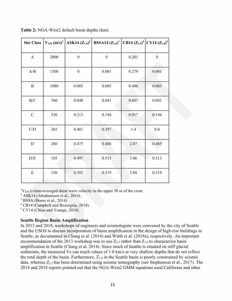
have the resolution to adequately characterize basin structure as parameterized by the GMMs. Therefore, we decided that it would not be appropriate to apply these models until better resolution maps and additional research are available. Our search found that detailed published community velocity models are available for four WUS urban regions: Los Angeles, San Francisco Bay area, Seattle, and Salt Lake City. We acquired digital files for: the Los Angeles area, model S4.26m01 (Lee et al., 2014) provided by SCEC; the USGS San Francisco Bay area (Aagaard et al., 2008); the Seattle region (Stephenson et al., 2007); and the Salt Lake City region (Magistrale et al., 2008). Figure 12 illustrates the boundaries of the four velocity models that we considered in the 2018 NSHM update for defining the depths to various velocity horizons along with some example velocity models. Basin factors used for crustal GMMs for basins in Los Angeles, San Francisco, and Salt Lake City areas The four NGA-West2 GMMs in the NSHM include empirical basin factors that are based on the depth at which a specified shear-wave velocity (Vs) is exceeded; Z1.0 is the depth at which Vs=1.0 km/s is exceeded, and Z2.5 is the depth at which Vs = 2.5 km/s is exceeded. Abrahamson et al. (2014), Boore et al. (2014), and Chiou and Youngs (2014) use Z1.0 while Campbell and Bozorgnia (2014; hereafter referred to as CB14) uses Z2.5. Table 2 shows the default basin depths calculated from the NGA-West2 GMMs based on VS30, which can be used when an independent estimate of the velocity horizon is not available. While basin effects are well known to be complex and influenced by many factors besides the depth of the basin at the location of the station, the GMM developers included this predictor variable because it explained some of the variability in the ground motions in the NGA-West2 database, particularly at longer periods. Figure 13 shows the basin amplification factors at 5s SA as a function of velocity horizon (Z1.0 or Z2.5) for each of the NGA-West2 GMMs, given a VS30. The vertical lines give the default basin depths for NEHRP site class boundary B/C (VS30 = 760 m/s; dashed black line) and NEHRP site class D (VS30 = 260 m/s; dashed gray line). For the GMMs using Z1.0, there is no amplification at the default basin depth. If the basin depth is greater than the default, the basin factors amplify the ground motion and if the basin depth is less, they deamplify the ground motion. For CB14, amplification is not dependent on VS30, and a Z2.5 value between 1 km and 3 km gives an amplification factor of 1.0.

15

Table 2: NGA-West2 default basin depths (km).

Site Class VS30 (m/s)1 ASK14 (Z1.0)2 BSSA14 (Z1.0)3 CB14 (Z2.5)4 CY14 (Z1.0)5

A 2000 0 0 0.201 0

A/B 1500 0 0.001 0.279 0.001

B 1080 0.005 0.005 0.406 0.005

B/C 760 0.048 0.041 0.607 0.041

C 530 0.213 0.194 0.917 0.194

C/D 365 0.401 0.397 1.4 0.4

D 260 0.475 0.486 2.07 0.485

D/E 185 0.497 0.513 3.06 0.513

E 150 0.502 0.519 3.88 0.519

1VS30 is time-averaged shear wave velocity in the upper 30 m of the crust. 2 ASK14 (Abrahamson et al., 2014). 3 BSSA (Boore et al., 2014). 4 CB14 (Campbell and Bozorgnia, 2014). 5 CY14 (Chiou and Youngs, 2014). Seattle Region Basin Amplification In 2013 and 2018, workshops of engineers and seismologists were convened by the city of Seattle and the USGS to discuss incorporation of basin amplification in the design of high-rise buildings in Seattle, as documented in Chang et al. (2014) and Wirth et al. (2018a), respectively. An important recommendation of the 2013 workshop was to use Z2.5 rather than Z1.0 to characterize basin amplification in Seattle (Chang et al. 2014). Since much of Seattle is situated on stiff glacial sediments, the measured Vs can reach values of 1.0 km/s at very shallow depths that do not reflect the total depth of the basin. Furthermore, Z1.0 in the Seattle basin is poorly constrained by seismic data, whereas Z2.5 has been determined using seismic tomography (see Stephenson et al., 2017). The 2014 and 2018 reports pointed out that the NGA-West2 GMM equations used California and other

16

international earthquakes when developing their basin amplification factors but did not have data from the Seattle region. There are very few strong-motion recordings in the NGA West 2 database that are located on deep basins and have VS30 values of 400-700 m/s, as is typical of Seattle’s glacial deposits. The Z1.0 values for much of the Seattle basin, based on the Stephenson et al. (2017) 3D velocity model, are often less than 500 m. According to the NGA West 2 GMMs that use Z1.0 in their basin terms, such sites should have little or no basin amplification. However, these sites are observed to have substantial basin amplification of factors of 2-3 relative to rock sites with similar VS30 values south of the Seattle basin, for crustal and intraslab earthquakes (e.g., Frankel et al., 2009; Chang et al., 2014). Use of basin terms for crustal earthquake GMMs for Seattle area For these reasons, we decided to use Z2.5 values, rather than Z1.0 values, to better account for basin-enhanced amplifications from crustal earthquakes. We want to use all of the NGA-West2 equations, and therefore need a Z1.0 value that is better tuned to ground motion amplification in the Seattle area. To this end, we calculate a Z1.0 value from Z2.5 using the NGA-West2 database to inform this conversion, similar to the equation derived by Campbell and Bozorgnia (2007). We regressed the Z1.0 and Z2.5 values in this database to obtain conversion relations that could be used for sites in and around the Seattle basin and that would be consistent with the NGA-West2 GMMs that apply the Z1.0 depth parameter. We only considered values for sites with appreciable sediment thicknesses (Z1.0 > 0.05 km and Z2.5 > 0.5 km) and did not use data that exhibited a strong independence between Zx values and ground shaking levels. The orthogonal regression assumes a linear relation and minimizes the Euclidean distance between the line and all points, through the sum of squared distances. Equal weights were assigned to each data point. Regressions to two data sets—the basin depths from the NGA-West2 database (Ancheta et al., 2013) and the basin depths from the most recent southern California seismic velocity model—provide two regression equations for obtaining Z1.0 from Z2.5 that are equally weighted in the 2018 model: Z1.0 = 0.1146Z2.5 + 0.2826 (1), Z1.0 = 0.0933Z2.5 + 0.1444 (2). The result of applying these models in the Seattle basin is to increase the Z1.0 values up to 1 km compared to the Z1.0 values from the basin velocity model. Modification of Subduction GMMs with basin terms for the Seattle region We used the CB14 basin terms based on Z2.5 to modify the subduction GMMs used in the NSHMs for earthquakes in the Cascadia subduction zone. To calculate ground shaking for the subduction events, we first removed the VS30 amplification term from the subduction GMMs to obtain the value for a reference rock site condition. With the rock subduction GMMs in hand, we add the VS30 -based site and Z2.5-based basin amplification terms from the CB14 GMM to obtain amplified ground shaking. We tested the impact of including the CB14 site term to the subduction GMMs, and results indicate less than 3% changes to hazard for firm rock sites (VS30 = 760 m/s) compared to the original models used in the 2014 NSHM. However, for softer soils (e.g., VS30 = 260 m/s) and longer periods (>1s) this new site term makes a more significant difference (20% increases for high accelerations up to 1.5g).

17

Recent 3D simulations for Cascadia M9 earthquakes show higher amplifications of long-period (1-10s) motions in the Seattle basin (factors of 2-3) than predicted from the Campbell and Bozorgnia (2014; factor of 1.5) and Chiou and Youngs (2014; factor of 1.2) GMMs, using Z2.5 and Z1.0 values from the Stephenson et al. (2017) velocity model (Frankel et al., 2018; Wirth et al., 2018b). These amplification factors are relative to a rock site just south of the basin. These higher amplifications of the simulations were consistent with observed amplifications from an earthquake located just below the plate interface (Frankel et al., 2018). While under predicting the observed amplification and that from the simulations, the CB14 basin term was larger than the Chiou and Youngs (2014) basin term, providing additional justification for preferring the CB14 term to be applied to subduction GMMs. We plan to consider the M9 simulation results in future updates of the NSHM. Hazard from Changes Caused from Considering Basin Effects Figure 14 shows a profile across the 2018 NHSM ground shaking model for Seattle that accounts for the sedimentary basin where basin depths from the local velocity model are greater than the default values calculated from the NGA-West2 GMMs for a VS30 of 500 m/s. The ground shaking for 5s SA at a site near Seattle has a default ground motion of about 0.11g and a basin-amplified motion of 0.17g, which represents a 0.06g difference and about a 55% increase (Fig. 14b). M9 simulation results are more than a factor of 2 higher than the NGA-West2 equations which depend on basin depth (Frankel et al., 2018). Similar ratios between basin-amplified and default ground motions for a VS30 of 260 m/s are also predicted in the deepest portions of the Los Angeles basins (e.g., Ventura Basin), San Francisco Bay area basins, and Salt Lake City area basins (Fig. 15). Relative to the 2014 NSHM, ground shaking hazard for the regions near Los Angeles, San Francisco, and Salt Lake City have increased or remained the same due to the assumptions discussed above. There is a minimal increase of ground motion in the city centers of Los Angeles and San Francisco, but for other locations within their metropolitan areas we see significantly increased ground shaking due to basin amplification (e.g., Long Beach and San Jose). Salt Lake City is in a generally shallower basin, and only a small area to the northwest of Salt Lake City shows amplified ground motions.

Final Seismic Hazard Maps

In this section, we discuss PGA as well as the 0.2s, 1s, and 5s SA hazard maps produced for a 2% probability of exceedance in 50 years and a firm rock site condition (VS30 = 760 m/s). Other maps, inputs, and hazard curves are available in the electronic supplement. The maps show high hazard along the western coast due to the San Andreas fault system and Cascadia Subduction Zone earthquakes, through the intermountain west seismic belt that is centered on the Wasatch and Teton faults, and at sites where historical earthquakes in New Madrid, Missouri and Charleston, South Carolina occurred more than a century ago (Fig. 16). Maps generated at 5s SA with VS30 = 260 m/s site conditions were not produced in previous versions of the NSHMs, due to limitations of the GMMs for the CEUS. In the new 5s models for soft soils (VS30 = 260 m/s), ground shaking has increased in the four urban areas by up to 40% compared to default ground motions, due to the influence of deep sedimentary basins. Changes to the model are caused by (1) earthquake catalogs, (2) CEUS GMMs, and (3) WUS basin amplified ground shaking. Part of the purpose of this paper is to identify why the ground motions

18

have changed relative to the 2014 NSHM, so we decompose the model to assess the locations where these three different components of the 2018 NSHM dominate. For this overview paper, we do not show all of the details of the further decomposition of the components that contribute to the changes in the ground shaking. This additional analysis is the subject of current research. Figure 17 shows 0.2s SA ground shaking on a uniform rock site of VS30 = 760 m/s for 2018 and 2014, along with the differences and ratios between the two maps to show where ground motions have changed. We find that in the CEUS ground motions increased in areas where new earthquakes occurred (e.g., Delaware, Ohio, Kansas) and decreased in areas where seismicity abated (e.g., northeast portion of the U.S.). We also find that seismicity rates decreased across the Intermountain West region; this has been attributed to the modification of magnitudes in the updated earthquake catalog. The ground shaking is elevated across a broad region within 1000 km of the NMSZ for 0.2s SA and 1s SA due to changes in the GMMs. Figure 18A shows 2018 and 2014 NSHM PGA total mean hazard curves (VS30 = 760 m/s), highlighting various exceedance levels considered in building designs over the years. The hazard is highest for the regions that have experienced large earthquakes and contain active fault sources capable of generating future earthquakes. Hazard is highest for sites in San Francisco, Los Angeles, and Seattle in the WUS and Memphis and Charleston in the CEUS. Ground motions are an order of magnitude or more lower in Chicago and New York City. Nevertheless, potential ground shaking could cause damage in either of these cities, but such shaking is not as likely. Figure 18B shows 5s total mean hazard curves (VS30 = 260 m/s) for a few sites in the WUS. At longer periods and softer soil sites, you can see the effect of basin amplification (relative to default basin depths) at Long Beach, San Jose, a site northwest of Salt Lake City, and Seattle. Table 3 shows the same sites as in Figure 17, but illustrates differences in PGA, 1s, and 5s SA total mean hazard that are caused by the updated seismicity catalog, CEUS GMMs, and the modification to WUS subduction GMMs. PGA ground motions are higher for the CEUS sites because of the new GMMs. Seismicity changes influence a few areas, such as Charleston, but these changes are much smaller than changes caused by the new GMMs. In the WUS, the 2018 NSHM updated subduction GMMs are very similar to those used in the 2014 NSHM, and we do not see many changes due to updating these GMMs. The updated seismicity catalog had some effect on areas in the Pacific northwest, as seen in Portland and Seattle. 1s SA ground motions show results similar to shorter periods, except changes in the seismicity catalog are not as large in the Pacific northwest. For the WUS sites only, we made the same comparisons at 5s SA for a NEHRP site class D (VS30 = 260 m/s). At longer periods and softer site conditions, the effect of the modification of the subduction GMMs can be seen at Portland and Seattle, as well as the changes in the total hazard from basin amplification, particularly at Seattle.

19

Table 3. Comparison of PGA, 1s, and 5s SA total mean hazard between the 2018 NSHM and 2014 NSHM when running the 2018 NSHM with the 2014 NSHM catalog and GMMs. Increases in hazard greater than 0.01g are highlighted in red. Decreases in hazard greater than 0.01g are highlighted in blue.

Site lon lat PGA, VS30 = 760 m/s1 1 Second, VS30 = 760 m/s1 5 Second, VS30 = 260 m/s2

Catalog GMMs Total Catalog GMMs Total Catalog GMMs Total

Chicago -87.7 41.9 0.001 0.013 0.014 0.000 0.010 0.011 N/A N/A N/A

St. Louis -90.2 38.6 0.016 0.055 0.073 0.001 0.026 0.028

New York City

-74 40.8 -0.007 0.004 -0.003 -0.001 -0.003 -0.004

Charleston -79.95 32.8 -0.014 0.177 0.166 -0.002 -0.023 -0.025

Memphis -90.1 35.2 0.007 0.131 0.138 0.001 0.013 0.014

Los Angeles -118.3 34.1 0.000 0.000 0.000 0.000 0.000 0.000 0.000 0.000 0.000

San Francisco

-122.4 37.8 0.000 0.000 0.000 0.000 0.000 0.000 0.000 0.001 0.001

Portland -122.7 45.5 -0.024 -0.004 -0.027 -0.007 0.003 -0.004 -0.001 0.027 0.025

Seattle -122.3 47.6 -0.012 -0.005 0.071 -0.007 0.004 0.225 -0.001 0.020 0.112

Salt Lake City

-111.9 40.8 -0.002 0.000 -0.007 -0.001 0.000 0.028 0.000 0.000 0.000

1 2% in 50 years probability of exceedance, NEHRP site class boundary B/C (VS30 = 760 m/s). 2 2% in 50 years probability of exceedance, NEHRP site class D (VS30 = 260 m/s).

Additional Periods and Site Classes For the 2014 NSHM, we were able to compute additional period and site class maps (Shumway et al., 2018), but they were completed too late for consideration in the building code. We were also only able to compute additional periods and site classes for the WUS, as the 2014 NSHM CEUS GMMs prevented calculations for long periods and soft soils. For the 2018 NSHM, we are now able to compute 22 periods and up to nine site classes (nine site classes in the CEUS, eight in the WUS).

20

Figure 19 shows response spectra for additional periods and site classes at selected sites across the U.S. WUS sites include Los Angeles, CA, San Francisco, CA, and Seattle, WA. The spectra at periods greater than about 0.2s SA for different VS30’s are evenly spaced, and accelerations increase with decreasing VS30. The CEUS sites include Charleston, SC Memphis, TN and New York, NY. The spectra for the CEUS sites look different than spectra for the WUS in that they: (1) have a sharper peak at 0.1s SA; (2) are unevenly spaced with varying VS30; and (3) exhibit decreased amplitudes between about 0.2 and 1s oscillator periods caused by the non-linear effects (Hashhash et al., 2017). The spectra at Charleston, SC and Memphis, TN have similar amplitudes at 0.1s compared to the sites in the WUS.

Changes in Earthquake Shaking, Exposure, and Risk

In this section, we discuss the shaking hazard and exposure analyses performed using most recent version of high resolution LandScan population exposure dataset produced by Oak Ridge National Laboratory (LandScan, 2017). In this, we consider the probabilistic PGA hazard curve at each site, assuming a reference site condition to be NEHRP site class B/C, which refers to VS30=760 m/s, and convert it into Modified Mercalli Intensity (MMI) hazard curve using Worden et al. (2012) intensity conversion relationship. Using log interpolation, we develop MMI hazard map for 50% (likely), 10% (infrequent) and 2% (rare but possible) intensities with probabilities of exceedance in 50 years as shown in Figure 20. The MMI values are obtained after rounding to an integer value, for example, numeric value of MMI 5.50 and 6.49 are rounded to intensity level of VI. Analogous to Jaiswal et al. (2015) study, we compared the MMI hazard and population exposure using most pertinent exposure datasets and provided an estimate of population exposure based on 1996, 2002, 2008, 2014 and 2018 hazard models. Changes in population exposure reflects both the geospatial change in population due to population growths as well as the spatial variation of changes in the estimates of seismic hazard, both of which have changed over time. Such analyses are not only helpful for discussing the changes in hazards (defined in terms of MMI, which are relatively easier to communicate) between different versions of hazard models but also for understanding their impact in terms of change in the number of people (a proxy for built environment) exposed to various levels of shaking hazards. The analyses show that earthquake shaking, and their impact are not limited to Californians or the larger west coast population but is spread over much wider geographic region. Clearly, more Americans are at risk to damaging levels of earthquake shaking than ever before (Table 4). As many as 34 million people (or 1 in 9) is expected to experience strong level of shaking at least once in their lifetime. Considering the ground shaking intensities that occur every ~475 years (i.e., 10% chance in 50 years), there has been significant increase in the number of people exposed to MMI VIII and above, i.e., from 28.0 million for the 2014 model to 32.2 million for the 2018 model. While the population growth from 2013 to 2017 is modest (~3%), this increase of 14% in exposure is mainly attributed due to the relatively larger area, mainly in CEUS, is estimated to experience damaging ground motions. Similarly, when considering low probability ground motions (2% chance in 50 years or ~2,475 recurrence interval), the exposure analysis shows one in three American is exposed to MMI VII and above, which reflect an increase of ~10% in human exposure between 2014 and 2018 hazard models. Such a level of increase is also evident for virtually all levels of shaking intensities indicating that the hazard has increased considerably between the two versions of the map.

21

Table 4. Estimated counts (in thousands) of population exposure* at various Modified Mercalli Intensity (MMI) shaking thresholds during different national probabilistic seismic hazard map cycles.

Map Year

Total Population Estimates at MMI

≥ V (Moderate Shaking)

≥ VI (Strong Shaking)

≥ VII (Very Strong Shaking)

≥ VIII (Severe Shaking)

≥ IX (Violent Shaking)

50% PE in 50 years (~72 years recurrence interval) 1996 41,844 31,945 19,827 1,935 19 2002 45,375 35,313 21,103 1,388 - 2008 45,045 34,001 16,490 97 - 2014 43,376 32,294 9,198 93 - 2018 45,812 34,474 11,731 108 -

10% PE in 50 years (~475 years recurrence interval) 1996 104,715 54,268 39,642 26,381 10,506 2002 104,591 59,463 44,109 29,967 9,336 2008 82,286 56,632 45,240 27,922 5,064 2014 97,597 62,685 47,259 28,061 3,969 2018 107,580 65,543 48,216 32,191 3,517

2% PE in 50 years (~2,475 years recurrence interval) 1996 235,236 164,769 95,654 45,393 30,051 2002 247,753 169,004 95,179 49,208 33,052 2008 241,898 155,909 84,193 49,558 32,021 2014 242,069 163,748 97,364 52,632 34,761 2018 267,712 184,021 107,017 57,778 38,608

* Population counts are estimates based on LandScan datasets for the conterminous U.S. and are rounded up to the nearest 1,000. The total population counts for the conterminous U.S. according to LandScan datasets are: LandScan 1998à268,411,000, LandScan 2003à288,883,000, LandScan 2009à304,937,000, LandScan 2013à313,940,000, and LandScan 2017à323,535,000.

Computer Codes and Implementation Details

For past NSHMs, we have calculated hazard, using a computer code written in Fortran. Recently, we have updated our seismic hazard computer code (nshmp-haz; https://doi.org/10.5066/F7ZW1K31) to modernize the code (the new code is written in Java) and allow for further improvements and capabilities. The new code is based on OpenSHA (Field et al., 2003) and available publicly on GitHub (https://github.com/usgs/nshmp-haz). The 2018 NSHM is also available on GitHub (https://github.com/usgs/nshm-cous-2018). Older source models (i.e., 2014 NSHM and the 2008

22

NSHM) are available on GitHub, as well, and can be run with the new code. We are in the process of converting additional older source models (e.g., Guam and the Northern Mariana Islands) into the new code, which will make updates to these models more straight forward. With the update to the new computer code, several changes to the way features are implemented in the code have changed. Table 5 lists these implementation changes. Table 5. List of nshmp-haz implementation changes, additions, and improvements.

Central and Eastern U.S.

● Implemented the NGA-East for USGS GMM, which includes mean model, site amplification, and aleatory variability logic trees leading to support for 22 spectral periods and site classes spanning 180 ≤ VS30 ≤ 3000 m/s.

Western U.S.

● Improved support for source model logic-tree and uncertainty management via the consolidation of fault sources representations.

● Added support for 22 spectral periods. ● Verified consistency of 2012 BC Hydro GMM (Addo et al., 2012; used in 2014 NSHM)

with Abrahamson et al. (2016).

General improvements and additions that support:

● Representations of ground motion model epistemic and aleatory variability to support NGA-East and consistent with the additional epistemic uncertainty model applied to NGA-West2 GMMs (Rezaeian et al., 2015).

● Deaggregation of multi-branch GMMs such as NGA-East. ● Computing hazard from 'cluster' source models using multi-branch GMMs. ● Improved internal representations of gridded-seismicity point-source models to reduce

small inconsistencies sometimes observed between static maps and dynamic calculations. ● New services for earthquake probability calculations. ● Ground motion post-processing, for example, to apply damping scaling factors other than

the fixed 5% that most GMMs implicitly consider (Rezaeian et al., 2014). ● GMM spectral period interpolation (used to fill out high frequencies). ● GMM spectral period extrapolation (ratio based and conditioned on having logic tree). ● Additional deaggregation epsilon bin metrics. ● Improved representation of UCERF3 contributing sources in deaggregations.

Conclusions We have updated the NSHM to a 2018 edition by applying an updated earthquake catalog, new GMMs for the CEUS, basin amplification terms for long periods in the WUS, and by updating our seismic hazard computer code. The ground motions are mostly higher across the CEUS due to new GMMs having higher sigma and amplification at periods less than about 2s. In the WUS, long-period shaking for soft soils is higher over the deepest portions of the sedimentary basins. This paper summarizes the data, methods, and models applied in the 2018 NSHM update, but does not provide

23

details regarding the implementation, sensitivity studies, implications, and products (e.g., additional periods, site classes, hazard curves, deaggregations) that are available in supplemental materials.

Acknowledgements Jill McCarthy, Bruce Worden, Jon Stewart, Grace Parker, Bill Stephenson, Gail Atkinson, Jon Ake, Working Groups that produced important inputs that are acknowledged within the paper, PEER, participants at the 2018 NSHM Update workshop, the NSHM Steering Committee, USGS editors and reviewers, Earthquake Spectra editors and reviewers, and the public who participated in the open comment period.

References

Aagaard, B. T., Brocher, T. M., Dolenc, D., Dreger, D., Graves, R. W., Harmsen, S., Hartzell, S., Larsen, S., McCandless, K., Nilsson, S., Petersson, N. A., Rodgers, A., Sjögreen B., and Zoback, M. L., 2008. Ground‐motion modeling of the 1906 San Francisco earthquake, part II: Ground‐motion estimates for the 1906 earthquake and scenario events, Bull. Seismol. Soc. Am. 98, 1012–1046, https://doi.org/10.1785/0120060410. Abrahamson, N.A., Silva, W.J., and Kamai, R., 2014. Summary of the ASK14 ground motion relation for active crustal regions, Earthquake Spectra 30 (3), 1025-1055, https://doi.org/10.1193/070913EQS198M. Abrahamson, N.A., Gregor, N., and Addo, K., 2016. BC Hydro ground motion prediction equations for subduction earthquakes, Earthquake Spectra 32 (1), 23-44, https://doi.org/10.1193/051712EQS188MR. Addo, K., Abrahamson, N, and Youngs, R., (BC Hydro), 2012. Probabilistic seismic hazard analysis (PSHA) model – Ground motion characterization (GMC) model: Report E658, published by BC Hydro. Al Atik, L., 2015. NGA-East: Ground-Motion Standard Deviation Models for Central and Eastern North America, PEER Report No. 2015/07, 217 pp, https://peer.berkeley.edu/sites/default/files/webpeer-2015-07-linda_al_atik.pdf. Alex, C.M. and Olsen, K.B., 1998, Lens-effect in Santa Monica? Geophys. Res. Letts. 25, 3441-3444. Algermissen, S. T., and Perkins, D. M., 1976. A Probabilistic estimate of the maximum acceleration in rock in the contiguous United States, U.S. Geological Survey Open-File Report 76–416, 2 plates, scale 1:7,500,000, 45 pp, https://doi.org/10.3133/ofr76416. Ancheta, T. D., Darragh, R. B., Stewart, J. P., Seyhan, E., Silva, W. J., Chiou, B. S.-J., Wooddell, K. E., Graves, R. W., Kottke, A. R., Boore, D. M., Kishida, T., and Donahue, J. L., 2013. PEER NGA-West2 Database, PEER Report No. 2013/03, Pacific Earthquake Engineering Research Center, University of California, Berkeley, CA, 134 pp,

24

https://peer.berkeley.edu/sites/default/files/webpeer-2013-03-timothy_d._ancheta_robert_b._darragh_jonathan_p._stewart_emel_seyhan.pdf. Atkinson, G. M., and Boore, D. M., 2003. Empirical ground-motion relations for subduction-zone earthquakes and their application to Cascadia and other regions, Bull. Seismol. Soc. Am. 93 (4), 1703-1729, https://doi.org/10.1785/0120020156. Atkinson, G.M., and Boore, D.M., 2008. Erratum to empirical ground-motion relations for subduction zone earthquakes and their application to Cascadia and other regions, Bull. Seismol. Soc. Am. 98 (5) 2567-2569, https://doi.org/10.1785/0120080108. Atkinson, G.M., and Boore, D.M., 2011. Modifications to existing ground-motion prediction equations in light of new data, Bull. Seismol. Soc. Am. 101 (3), 1121-1135, https://doi.org/10.1785/0120100270. Boore, D.M., Stewart, J.P., Seyhan, E., and Atkinson, G.M., 2014. NGA-West2 equations for predicting PGA, PGV, and 5% damped PSA for shallow crustal earthquakes, Earthquake Spectra 30 (3), 1057-1085, https://doi.org/10.1193/070113EQS184M. Campbell, K.W. and Bozorgnia, Y., 2007. Campbell-Bozorgnia NGA ground motion relations for the geometric mean and horizontal component of peak and spectral ground motion parameters, PEER Report No. 2007/02, 240 pp, https://peer.berkeley.edu/sites/default/files/web_peer702_kenneth_w._campbell_yousef_bozorgnia.pdf. Campbell, K. W., and Bozorgnia, Y., 2014. NGA-West2 ground motion model for the average horizontal components of PGA, PGV, and 5% damped linear acceleration response spectra, Earthquake Spectra 30 (3), 1087–1115, http://dx.doi.org/10.1193/062913EQS175M. CEUS–SSCn, 2012. Central and Eastern United States seismic source characterization for nuclear facilities, Palo Alto, California, EPRI, U.S. DOE, and U.S. NRC, [variously paged]. (Also available at, http://www.ceus-ssc.com/Report/Downloads.html.) Chang, S. W., Frankel, A. D., and Weaver, C. S., 2014. Report on workshop to incorporate basin response in the design of tall buildings in the Puget Sound region, Washington, U.S. Geological Survey Open-File Report 2014–1196, 28 pp, http://dx.doi.org/10.3133/ofr20141196. Chiou, B.,S.-J., and Youngs, R.R., 2014. Update of the Chiou and Youngs NGA model for the average horizontal component of peak ground motion and response spectra, Earthquake Spectra 30 (3), 1117-1153, https://doi.org/10.1193/072813EQS219M. Cornell, C. A., 1968. Engineering seismic risk analysis, Bull. Seismol. Soc. Am. 58, 1583–1606, https://pubs.geoscienceworld.org/ssa/bssa/article/58/5/1583/116673/engineering-seismic-risk-analysis.

25

Davis, P.M., Rubinstein, J.L., Liu, K.H., Gao, S.S., and Knopoff, L. 2000, Northridge earthquake damage caused by geologic focusing of seismic waves, Science, 289 (5485), 1746-1750, https://doi.org/10.1126/science.289.5485.1746. Dobson, J.E., Bright, E.A., Coleman, PR., Durfee, R.C., and Worley, B.A., 2000. LandScan: A global population database for estimating populations at risk, Photogrammetric Engineering & Remote Sensing 66, 849-857. Electrical Power Research Institute (EPRI), 2013. EPRI (2004, 2006) Ground-Motion Model (GMM) review project, EPRI Report No. 3002000717, Palo Alto, California, 67 pp, https://www.nrc.gov/docs/ML1317/ML13170A385.pdf. Field, E. H., Jordan, T. H., and Cornell, C. A., 2003. OpenSHA: A developing community-modeling environment for seismic hazard analysis, Seismol. Res. Lett. 74 (4), 406-419, https://doi.org/10.1785/gssrl.74.4.406. Field, E. H., 1996. Spectral amplification in a sediment-filled valley exhibiting clear basin-edge-induced waves, Bull. Seismol. Soc. Am. 86 (4), 991-1005, https://pubs.geoscienceworld.org/ssa/bssa/article/86/4/991/120109/spectral-amplification-in-a-sediment-filled-valley. Field, E.H., Arrowsmith, R.J., Biasi, G.P., Bird, P., Dawson, T.E., Felzer, K.R., Jackson, D.D., Johnson, K.M., Jordan, T.H., Madden, C., and Michael, A.J., 2014. Uniform California earthquake rupture forecast, version 3 (UCERF3) – The time-independent model, Bull. Seismol. Soc. Am. 104 (3), 1122-1180, https://doi.org/10.1785/0120130164. Frankel, A., 1995. Mapping seismic hazard in the Central and Eastern United States, Seismol. Res. Lett. 66 (4), 8-21, https://doi.org/10.1785/gssrl.66.4.8. Frankel, A., Mueller, C., Barnhard, T., Perkins, D., Leyendecker, E. V., Dickman, N., Hanson, S., and Hopper, M., 1996. National Seismic Hazard Maps—Documentation June 1996, U.S. Geological Survey Open-File Report 96-532, 110 pp, https://pubs.usgs.gov/of/1996/532/. Frankel, A., Wirth, E., Marafi, N., Vidale, J., and Stephenson, W., 2018. Broadband synthetic seismograms for magnitude 9 earthquakes on the Cascadia megathrust based on 3D simulations and stochastic synthetics, Part 1: Methodology and overall results, Bull. Seismol. Soc. Am. 108 (5A), 2347-2369, https://doi.org/10.1785/0120180034. Frankel, A., Stephenson, W. and Carver, D. (2009). Sedimentary basin effects in Seattle, Washington: ground-motion observations and 3D simulations, Bull. Seism. Soc. Am. 99, 1579-1611, https://doi.org/10.1785/0120080203. Frankel, A. D., Carver, D. L., and Williams R. A., 2002a. Nonlinear and linear site response and basin effects in Seattle for the M 6.8 Nisqually, Washington, earthquake, Bull. Seism. Soc. Am. 92 (6), 2090-2109, https://doi.org/10.1785/0120010254.

26

Frankel, A.D., Petersen, M.D., Mueller, C.S., Haller, K.M., Wheeler, R.L., Leyendecker, E.V., Wesson, R.L., Harmsen, S.C., Cramer, C.H., Perkins, D.M., and Rukstales, K.S., 2002b. Documentation for the 2002 update of the national seismic hazard maps, US Geological Survey Open-File Report 02-420, 33 pp, https://pubs.usgs.gov/of/2002/ofr-02-420/OFR-02-420.pdf. Gardener, J.K., and Knopoff, L., 1974. Is the sequence of earthquakes in Southern California, with aftershocks removed, Poissonian?, Bull. Seismol. Soc. Am. 64 (5), 1363-1367. Goulet, C. A., Bozorgnia, Y., Kuehn, N., Al Atik, L., Youngs, R. R., Graves, R. W., and Atkinson G. M., 2017. NGA-East ground-motion models for the U.S. Geological Survey National Seismic Hazard Maps, PEER Report No. 2017/03, 207 pp, https://peer.berkeley.edu/sites/default/files/christine-a-goulet-yousef-bozorgnia-2017_03_0.pdf (and 12 pp addendum: https://peer.berkeley.edu/sites/default/files/peer-2017-03_addendum.pdf). Graizer, V., 2016. Ground‐motion prediction equations for central and eastern North America, Bull. Seismol. Soc. Am. 106, 1600-1612, https://doi.org/10.1785/0120150374. Graizer, V., 2017. Alternative (G-16v2) ground-motion prediction equations for central and eastern North America, Bull. Seismol. Soc. Am. 107 (2), 869-886, https://doi.org/10.1785/0120160212. Graves, R.W., Pitarka, A., and Sommerville, P.G., 1998. Ground-motion amplification in the Santa Monica area: Effects of shallow basin structure, Bull. Seismol. Soc. Am. 88, 1224-1242. Graves, R., Jordan, T.H., Callaghan, S., Deelman, E., Field, E., Juve, G., Keeselman, C., Maechling, P., Mehta, G., Milner, K., and Okaya, D., 2011. Cybershake: A physics-based seismic hazard model for southern California, Pure. Appl. Geophys. 168 (3-4) 367-381, https://doi.org/10.1007/s00024-010-0161-6. Hashash, Y. M. A., Harmon, J. A., Iihan, O., Parker, G. A., and Stewart, J. P., 2017. Recommendation for ergodic nonlinear site amplification in central and eastern North America, PEER Report No. 2017/05, 79 pp., https://peer.berkeley.edu/sites/default/files/youssef-m-a-hashash-joseph-harmon-okan-ilhan-2017_05.pdf. Helmstetter, A., Kagan, Y. Y., and Jackson, D. D., 2007. High-resolution time-independent gridbased forecast for M ≥ 5 earthquakes in California, Seismol. Res. Lett. 78 (1), 78–86, https://doi.org/10.1785/gssrl.78.1.78. Idriss, I.M., 2014. An NGA-West2 empirical model for estimating the horizontal spectral values generated by shallow crustal earthquakes, Earthquake Spectra 30 (3), 1155-1177, https://doi.org/10.1193/070613EQS195M. Jaiswal, K. S., Petersen, M. D., Rukstales, K., and Leith, W. S., 2015. Earthquake shaking hazard estimates and exposure changes in the conterminous United States, Earthquake Spectra 31 (S1), S201-S220, https://doi.org/10.1193/111814EQS195M.

27

Jaiswal, K., Bausch, D., Rozelle J., Holub, J., and McGowan, S., 2017. Hazus® estimated annualized earthquake losses for the United States, Federal Emergency Management Agency Report P-366, 78 pp, http://pubs.er.usgs.gov/publication/70189832. LandScanTM database, 2017. High resolution global population data set [LS1998, LS2003, LS2009, LS2013, LS2017], UT-Battelle, LLC, at Oak Ridge National Laboratory, http://www.ornl.gov/landscan/, last accessed on Nov 6, 2018. Lee, E.-J., Chen, P., Jordan, T. H., Maechling, P. J., Denolle, M., and Beroza, G. C., 2014. Full‐3‐D tomography for crustal structure in southern California based on the scattering‐integral and the adjoint‐wavefield methods, J. Geophys. Res. 119, 6421–6451, https://doi.org/10.1002/2014JB011346. Luco, N., Bachman, R.E., Crouse, C.B., Harris, J.R., Hooper, J.D., Kircher, C.A., Caldwell, P.J., and Rukstales, K.S., 2015. Updates to building-code maps for the 2015 NEHRP recommended seismic provisions, Earthquake Spectra 31 (S1), S245-S271, https://doi.org/10.1193/042015EQS058M. Magistrale, H., Olsen, K. B., and Pechmann, J. C., 2008. Construction and verification of a Wasatch Front Community Velocity Model, U.S. Geological Survey Technical Report 06HQGR0012. McNamara, D.E., Petersen, M.D., Thompson, E.M., Powers, P.M., Shumway, A.M., Hoover, S.M., Moschetti, M.P., and Wolin, E., 2018. Evaluation of ground motion models for USGS seismic hazard forecasts: Induced and tectonic earthquakes in the Central and Eastern U.S., Seism. Soc. Am. Bull., in press. Moschetti, M. P., 2015. A long-term earthquake rate model for the central and eastern United States from smoothed seismicity. Bull. Seismol. Soc. Am. 105 (6), 2928-2941, https://doi.org/10.1785/0120140370. Moschetti, M. P., Powers, P. M., Petersen, M. D., Boyd, O. S., Chen, R., Field, E. H., Frankel, A. D., Haller, K. M., Harmsen, S. C., Mueller, C. S., and Wheeler, R.L., 2015. Seismic source characterization for the 2014 update of the US national seismic hazard model. Earthquake Spectra 31 (S1), S31-S57, https://doi.org/10.1193/110514EQS183M. Moschetti, M. P., Hartzell, S., Ramírez‐Guzmán, L., Frankel, A. D., Angster, S. J., and Stephenson, W. J., 2017. 3D Ground‐Motion Simulations of Mw 7 Earthquakes on the Salt Lake City Segment of the Wasatch Fault Zone: Variability of Long‐Period (T≥ 1 s) Ground Motions and Sensitivity to Kinematic Rupture Parameters. Bull. Seismol. Soc. Am. 107 (4), 1704-1723, https://doi.org/10.1785/0120160307. Mueller, C. S., 2018. Earthquake catalogs for the USGS National Seismic Hazard Maps, Seismol. Res. Lett., https://doi.org/10.1785/0220170108. nshmp-haz, 2017. National Seismic Hazard Model Project Computer Code (nshmp-haz), https://doi.org/10.5066/F7ZW1K31.

28

Pacific Earthquake Engineering Research Center (PEER), 2015. NGA-East: Adjustments to Median Ground-Motion Models for Central and Eastern North America, PEER Report No. 2015/08, 129 pp, https://peer.berkeley.edu/sites/default/files/webpeer-2015-08-nga-east-_adjustments_to_median_ground-motion_models_for_central_and_eastern_north_america.pdf. Petersen, M.D., Bryant, W.A., Cramer, C.H., Cao, T., Reichle, M, Frankel, A.D., Lienkaemper, J.J., McCrory, P.A., and Schwartz, D.P., (1996). Probabilistic seismic hazard assessment for the state of California, U.S. Geological Survey Open-file Report, 96-706, 56 pp. Petersen, M. D., Frankel, A. D., Harmsen, S. C., Mueller, C. S., Haller, K. M., Wheeler, R. L., Wesson, R. L., Zeng, Y., Boyd, O. S., Perkins, D. M., Luco, N., Field, E. H., Wills, C. J., and Rukstales, K. S., 2008. Documentation for the 2008 update of the United States National Seismic Hazard Maps, U.S. Geological Survey Open-File Report 2008–1128, 61 pp, https://doi.org/10.3133/ofr20081128. Petersen, M. D., Moschetti, M. P., Powers, P .M., Mueller, C. S., Haller, K. M., Frankel, A. D., Zeng, Y., Rezaeian, S., Harmsen, S. C., Boyd, O. S., Field, N., Chen, R., Rukstales, K. S., Luco, N., Wheeler, R. L., Williams, R. A., and Olsen, A. H., 2014. Documentation for the 2014 update of the United States National Seismic Hazard Maps, U.S. Geological Survey Open-File Report 2014–1091, 243 pp, https://dx.doi.org/10.3133/ofr20141091. Petersen, M. D., Moschetti, M. P., Powers, P. M., Mueller, C. S., Haller, K. M., Frankel, A. D., Zeng, Y., Rezaeian, S., Harmsen, S. C., Boyd, O. S., Field, N., Chen, R., Rukstales, K. S., Luco, N., Wheeler, R. L., Williams, R. A., and Olsen, A. H., 2015. The 2014 United States National Seismic Hazard Model, Earthquake Spectra 31 (S1), S1-S30, https://doi.org/10.1193/120814EQS210M. Petersen, M.D., Mueller, C.S., Moschetti, M.P., Hoover, S.M., Llenos, A.L., Ellsworth, W.L., Michael, A.J., Rubinstein, J.L., McGarr, A.F., and Rukstales, K.S., 2016a. 2016 one-year seismic hazard forecast for the central and eastern United States from induced and natural earthquakes, U.S. Geological Survey Open-File Report 2016-1035, 52 pp, http://dx.doi.org/10.3133/ofr20161035. Petersen, M.D., Mueller, C.S., Moschetti, M.P., Hoover, S.M., Llenos, A.L., Ellsworth, W.L., Michael, A.J., Rubinstein, J.L., McGarr, A.F., and Rukstales, K.S., 2016b. Seismic-hazard forecast for 2016 including induced and natural earthquakes in the central and eastern United States, Seismol. Res. Lett. 87 (6), 1327-1341, https://doi.org/10.1785/0220160072. Petersen, M.D., Mueller, C.S., Moschetti, M.P., Hoover, S.M., Rukstales, K.S., McNamara, D.E., Williams, R.A., Shumway, A.M., Powers, P.M., Earle, P.S., and Llenos, A.L., 2018. 2018 one-year seismic hazard forecast for the central and eastern United States from induced and natural earthquakes, Seismol. Res. Lett. 89 (3), 1049-1061, https://doi.org/10.1785/0220180005. Pratt, T.L., Brocher, T.M., Weaver, C.S., Miller, K.C., Trehu, A.M., Creager, K.C., Crossen, R.S., and Snelson, C.M., 2003. Amplification of seismic waves by the Seattle basin, northwestern U.S., Bull. Seismol. Soc. Am. 93, 533-545.

29

Rezaeian, S., Bozorgnia, Y., Idriss, I.M., Campbell, K., Abrahamson, N., and Silva, W., 2014. Damping scaling factors for elastic response spectra for shallow crustal earthquakes in active tectonic regions: “Average” horizontal component, Earthquake Spectra 30 (2), 939-963, https://doi.org/10.1193/100512EQS298M. Rezaeian, S., Petersen, M. D., and Moschetti, M. P, 2015. Ground motion models used in the 2014 U.S. National Seismic Hazard Maps, Earthquake Spectra 31 (S1), S59-84, http://doi.org/10.1193/111714EQS194M. Roten, D., Olsen, K. B., Pechmann, J. C., Cruz-Atienza, V. M., and Magistrale, H., 2011. 3D simulations of M 7 earthquakes on the Wasatch fault, Utah, Part I: Long-period (0–1 Hz) ground motion, Bull. Seismol. Soc. Am. 101 (5), 2045-2063, https://doi.org/10.1785/0120110031. Shahjouei A., and Pezeshk S., 2016. Alternative hybrid empirical ground-motion model for central and eastern North America using hybrid simulations and NGA-West2 models, Bull. Seismol. Soc. Am. 106 (2), 734-754, https://doi.org/10.1785/0120140367. Shumway, A. M., Petersen, M. D., Powers, P. M., and Rezaeian, S., 2018. Additional period and site class maps for the 2014 National Seismic Hazard Model for the conterminous United States, U.S. Geological Survey Open-File Report 2018–1111, 46 pp, https://doi.org/10.3133/ofr20181111. Stephenson, W. J., 2007. Velocity and density models incorporating the Cascadia subduction zone for 3D earthquake ground motion simulations, U.S. Geological Survey Open-File Report 2007–1348, Version 1.3, 24 pp, https://doi.org/10.3133/ofr20071348. Stephenson, W. J., Reitmann, N. G., and Angster, S. J., 2017. P- and S-wave velocity models incorporating the Cascadia subduction zone for 3D earthquake ground motion simulations— Update for OFR 2007-1348, U.S. Geological Survey Open-File Report 2017–1152, 40 pp, https://doi.org/10.3133/ofr20171152. Stephenson, W.J., Frankel, A.D., Odum, J.K., Williams, R.A., and Pratt, T.L. (2006). Toward resolving an earthquake ground motion mystery in West Seattle, Washington State: shallow seismic focusing may cause anomalous chimney damage, Geophys. Res. Letts. 33, L06316, https://doi.org/10.1029/2005GL025037. Stewart, J. P., Parker, G. A., Harmon, J. A., Atkinson, G. M., Boore, D. M., Darragh, R. B., Silva, W. J., and Hashash, Y. M. A., 2017. Expert panel recommendations for ergodic site amplification in central and eastern North America, PEER Report No. 2017/04, 81 pp, https://peer.berkeley.edu/sites/default/files/jonathan-p-stewart-grace-a-parker-2017_04.pdf. Werner, M.J., Helmstetter, A., Jackson, D.D., and Kagan, Y.Y., 2011. High-resolution long-term and short-term earthquake forecasts for California, Bull. Seismol. Soc. Am. 101 (4), 1630-1648, https://doi.org/10.1785/0120090340.

30

Wirth, E. A., Chang, S. W., and Frankel, A. D., 2018a. 2018 report on incorporating sedimentary basin response into the design of tall buildings in Seattle, Washington, U.S. Geological Survey Open-File Report 2018–1149, 19 pp, https://doi.org/10.3133/ofr20181149. Wirth, E. A., Frankel, A. D., Marafi, N., Vidale, J. E., Stephenson, W. J., 2018b. Broadband synthetic seismograms for magnitude 9 earthquakes on the Cascadia megathrust based on 3D simulations and stochastic synthetics, Part 2: Rupture parameters and variability, Bull. Seismol. Soc. Am. 108 (5A), 2370–2388, https://doi.org/10.1785/0120180029. Worden, C. B., Gerstenberger, M. C., Rhoades, D. A., and Wald, D. J., 2012. Probabilistic relationships between ground motion parameters and modified Mercalli intensity in California, Bull. Seism. Soc. Am. 102 (1), 204-221, https://doi.org/10.1785/0120110156.

APPENDICES

Appendix A - Memorandum on Sigma to NSHMP from Stewart et al. (July 13, 2018) Appendix B - Memorandum on Amplification Factors to NSHMP from Stewart et al. (July 18, 2018 [updated July 26, 2018])

Memorandum

Date: July 13, 2018 To: The USGS National Seismic Hazard Mapping Project From: Jonathan P. Stewart, Grace A. Parker, Linda Al Atik, Gail M. Atkinson, Christine Goulet RE: Modified φS2S model for CENA

During the March 7, 2018 USGS workshop on the national seismic hazard maps, there was discussion of what aleatory variability model should be used with the NGA-East site factors provided in Stewart et al. (2017). The writers of this memo were asked by Mark Petersen to examine this issue in an email sent on 3/16/2018. After several web meetings and related work, we provided a model in a Power Point file that was sent to USGS on April 24, 2018. That model provided values of site-to-site variability (φS2S), which is a component of within-event variability (φ), which in turn is a component of overall variability (σ) used in hazard calculations. All uncertainty components other than φS2S were unchanged from earlier recommendations provided in a PEER report by Goulet et al. (2017).

The model for φS2S that was originally provided is given by:

𝜙𝜙𝑆𝑆2𝑆𝑆 = 𝜙𝜙𝑆𝑆2𝑆𝑆(𝐌𝐌 < 𝐌𝐌1) + �0 𝐌𝐌 < 𝐌𝐌1

𝛥𝛥𝛥𝛥𝑆𝑆2𝑆𝑆𝛥𝛥𝐌𝐌

(𝐌𝐌−𝐌𝐌1) 𝐌𝐌1 < 𝐌𝐌 < 𝐌𝐌1 + 𝛥𝛥𝐌𝐌𝛥𝛥𝜙𝜙𝑆𝑆2𝑆𝑆 𝐌𝐌 > 𝐌𝐌1 + 𝛥𝛥𝐌𝐌

(1)

where φS2S (M < M1) is a VS30-dependent model for small magnitudes and ∆φS2S, ∆M, and M1 are parameters that are required to express magnitude-dependence. The φS2S (M < M1) term was given by:

𝜙𝜙𝑆𝑆2𝑆𝑆(𝐌𝐌 < 𝐌𝐌1) =

⎩⎨

⎧𝜙𝜙𝑆𝑆2𝑆𝑆,1 𝑉𝑉𝑆𝑆30 < 𝑉𝑉𝛥𝛥1

𝜙𝜙𝑆𝑆2𝑆𝑆,1 −�𝛥𝛥𝑆𝑆2𝑆𝑆,1−𝛥𝛥𝑆𝑆2𝑆𝑆,2�

𝑉𝑉𝜙𝜙2−𝑉𝑉𝜙𝜙1�𝑉𝑉𝑆𝑆30 − 𝑉𝑉𝛥𝛥1� 𝑉𝑉𝛥𝛥1 < 𝑉𝑉𝑆𝑆30 < 𝑉𝑉𝛥𝛥2

𝜙𝜙𝑆𝑆2𝑆𝑆,2 𝑉𝑉𝑆𝑆30 > 𝑉𝑉𝛥𝛥2

(2)

where 𝜙𝜙𝑆𝑆2𝑆𝑆,1, 𝜙𝜙𝑆𝑆2𝑆𝑆,2, Vφ1, and Vφ2 are parameters required to express VS30-dependence.

USGS staff, including Art Frankel, Mark Peterson, Peter Powers, Allison Shumway, and

Sanaz Rezaeian, expressed concerns regarding several aspects of the φS2S model as given in Eqs. (1) and (2). One concern was that the total φ for CENA at long periods was lower than in the western US, which is caused by empirical φS2S values derived from NGA-East data being lower than those from the western US for comparable magnitudes (Goulet et al. 2017, Figure 5.5). The second concern was that the magnitude-dependence of total φ for CENA is too large, which caused total σ at large magnitudes to be too small for short oscillator periods.

We found these concerns to be persuasive and have reconsidered both aspects of the original model. We begin with the second issue, concerning magnitude-dependence. The original φS2S model adopted ∆φS2S values derived from western US data using the NGA-West2 GMMs. Those values were negative at short periods and positive at long periods, with the transition occurring at about 1.0 sec oscillator period. When combined with the magnitude-dependent φss models in Goulet et al. (2017), the overall magnitude dependence of φ is excessive.

To correct for this, we now target the magnitude dependence of the total φ model given in

Table 5.5 of Goulet et al. (2017). It is important to note here that we do not target the φ values in that table, just their magnitude dependence (difference between the values for M 5 and M 7). To develop these new ∆φS2S values, we computed the change in 𝜙𝜙𝑆𝑆2𝑆𝑆,1 (which are empirically constrained from CENA data) that would be required for large M to match the change in φ values between M 5 and 7. These computations used the M-dependent global φss model given in Table 5.2 of Goulet et al. (2017) (i.e., in that table, the M-dependence was taken as by b minus a for the central branch). We found that the M-dependent global φss model provides levels of M-dependence in total φ that nearly match the target from Table 5.5 of Goulet et al. (2017). The additional magnitude-dependence of ∆φS2S that would be required for a perfect match range from -0.019 to +0.067. The absolute values for many periods (including PGA and PGV) are below 0.01. Accordingly, our judgment is that the M-dependent φss model is sufficient to capture the M-dependence of total φ model.

As a result of this simplification, the φS2S model can now be expressed as:

𝜙𝜙𝑆𝑆2𝑆𝑆 =

⎩⎨

⎧𝜙𝜙𝑆𝑆2𝑆𝑆,1 𝑉𝑉𝑆𝑆30 < 𝑉𝑉𝛥𝛥1

𝜙𝜙𝑆𝑆2𝑆𝑆,1 −�𝛥𝛥𝑆𝑆2𝑆𝑆,1−𝛥𝛥𝑆𝑆2𝑆𝑆,2�

𝑉𝑉𝜙𝜙2−𝑉𝑉𝜙𝜙1�𝑉𝑉𝑆𝑆30 − 𝑉𝑉𝛥𝛥1� 𝑉𝑉𝛥𝛥1 < 𝑉𝑉𝑆𝑆30 < 𝑉𝑉𝛥𝛥2

𝜙𝜙𝑆𝑆2𝑆𝑆,2 𝑉𝑉𝑆𝑆30 > 𝑉𝑉𝛥𝛥2

(3)

To address the first issue, we have modified the coefficients for 𝜙𝜙𝑆𝑆2𝑆𝑆,1 to match values from western US sites for oscillator periods of 0.3 and greater using data over the full magnitude range from that data set. No changes were made to 𝜙𝜙𝑆𝑆2𝑆𝑆,2, Vφ1, or Vφ2. Figure 1 plots the current values of 𝜙𝜙𝑆𝑆2𝑆𝑆,1 along with the previous values. Values of 𝜙𝜙𝑆𝑆2𝑆𝑆,2 are also shown for completeness. Figure 2 plots the period-dependence of φ for magnitudes of 5 and 7 as given in Table 5.5 of Goulet et al. (2017) and from the present model. For the present model, φss is taken from Table 5.2 of Goulet et al. (2017) (global model, central branch). The principle change is that the present model has higher φ values for short periods (≤ ∼ 1.5 sec). This increase in φ is what was discussed during the March 7 2018 USGS workshop as being needed to account for the impact of site effects. Values of φ are smaller at long periods. Coefficients for the revised model are given in a spreadsheet.

Figures 3 and 4 show comparisons of total aleatory σ for magnitudes 5 and 7 as given in the present recommendations, the model provided in Table 5.5 of Goulet et al. (2017), and the 2013 EPRI model. The results labelled as ‘present recommendations’ in Figures 3 and 4 use M-dependent τ from Table 5.5 of Goulet et al. (2017), M-dependent φss from Table 5.2 of Goulet et

al. (2017) (global model, central branch), and take 𝜙𝜙𝑆𝑆2𝑆𝑆 = 𝜙𝜙𝑆𝑆2𝑆𝑆,1 as provided here. The higher standard deviation at short periods is caused by the increase in 𝜙𝜙𝑆𝑆2𝑆𝑆. We recognize that there are modest decreases at periods longer than about 0.7-1.5 sec, which are due to differences in φ as observed in Figure 2; we consider the values provided here to be more credible.

Figure 1. Site-to-site standard deviation values (𝜙𝜙𝑆𝑆2𝑆𝑆,1 and 𝜙𝜙𝑆𝑆2𝑆𝑆,2) from current and previous models.

Figure 2. Comparison of total φ values for magnitudes of 5 and 7 from Goulet et al. (2017) and present recommendations.

Figure 3. Comparison of σ models as a function of oscillator period from the present recommendations, Goulet et al. (2017), and EPRI (2013) for magnitude 5.

Figure 4. Comparison of σ models as a function of oscillator period from the present recommendations, Goulet et al. (2017), and EPRI (2013) for magnitude 7.

Memorandum

Date: July 18, 2018 (updated July 26 2018) To: The USGS National Seismic Hazard Mapping Project From: Jonathan P. Stewart, Grace A. Parker, Youssef M.A. Hashash, Gail M. Atkinson, David

M. Boore, Robert B. Darragh, Walter J. Silva, Okan Ilhan and Joseph A. Harmon RE: Proposed Recommendations to the USGS on 3000 to 760 m/s Site Amplification Factors

and Related Issues F760 term

As part of the USGS National Seismic Hazard Mapping Project, Art Frankel, Mark Peterson, Peter Powers, Allison Shumway, and Sanaz Rezaeian have expressed concerns regarding the F760 term in the recommended site amplification model provided in Stewart et al. (2017) (hereafter Sea17) for central and eastern north America (CENA). This F760 term is meant to represent the amplification of 5% damped response spectral ordinates between reference conditions of 3000 and 760 m/s, which is required for compatibility with NGA-East ground motion models (GMMs).

The F760 term provided in Sea17 is based on models developed using simulations from

Harmon et al. (2018), Boore and Campbell (2017), and Darragh et al. (2015). The majority of shear wave velocity (VS) profiles used in the simulations produced a peak amplification at 0.1s (10 Hz), resulting in an observed peak in our recommended model (Figure 1). However, not all models showed this peak, including one of the Darragh et al. (2015) models (labeled ‘PEA – Gradient’ in Figure 1). Additionally, upon further literature review we found computations of site amplification using a VS profile with a relatively gradual gradient that was originally used in Frankel et al. (1996) and later applied in Atkinson and Boore (2006). Both the Darragh et al. (2015) gradient VS profile and the Frankel et al. (1996) VS profile lack a strong impedance contrast and are referred to subsequently as “gradient” profiles. Figure 2 shows F760 amplification as a function of oscillator period for these models. In the case of the Frankel et al. (1996) profile, simulations were re-done by the 5th author for various magnitude and distance combinations and for site κ = 0.01 and 0.02 sec.

The recommendations for F760 from Sea17 were weighted towards the models that

produce a strong peak at 0.1s. Because the Sea17 modeling framework adds F760 to Fv for all input VS30 values, this peak at 0.1s is observed across all site conditions, which may or may not represent reality. Accordingly, we examined both empirically and through simulations whether or not the 0.1s peak observed in the Sea17 recommended model is also observed in the CENA ground motions. NGA-East data was used to evaluate typical empirical spectral shapes for different VS30 values. After binning by earthquake magnitude (M), rupture distance (RRUP), and VS30, the available spectra were normalized by the average PSA between 0.08 and 1.5s oscillator periods. The spectral shapes for M = 4-5.5, RRUP = 0-150 km and VS30 bins around 2000, 760, 500, and 260m/s are shown in Figures 3-6. The data show a strong peak near 0.1s in the mean

spectral shape for VS30 values 500 m/s or more, and a peak near 0.25s at 260 m/s. These trends match those noted by Hassani and Atkinson (2016) in the NGA-East data, in which the peak of H/V (a proxy for site amplification) is near 0.1 s (10 Hz) for sites with VS30 values in the range from 500 m/s to 1000 m/s, as shown in Figure 7; note also the systematic trend to lower frequencies of peak response with decreasing shear-wave velocity.

In addition to the use of information from recordings, we queried the database of

simulation results in Harmon et al. (2018). The query was made for sites with VS30 near 760, 500, and 260 m/s, and the mean spectra were computed and normalized in the same manner as the empirical spectra. These normalized spectra are shown in Figure 8. The results agree with the empirical results at VS30 values of 760 and 500m/s, and also support the shift in the peak response to longer periods at slower VS30. Perhaps because these amplification factors were developed using VS profiles with impedance contrasts, a peak near 0.1s is observed at all values of VS30, which is different from the empirical result for the 260 m/s bin.

The results from these analyses indicate that the peaked F760 is representative for at least

a portion of sites in CENA. We believe this is due to sites with higher VS30 tending to have rock near the ground surface overlain by a shallow soil layer, creating a velocity impedance and thus a strongly peaked response. However, sites with lower VS30 values where 760m/s occurs at depth may be more likely to have gradual “gradient” increase in VS30 in a weathered rock zone at depth. For these sites, a peaked F760 model may not be representative. Thus, a first order method for distinguishing between these impedance and gradient sites is proposed that is based on the ground-surface VS30. Our interpretation of these results is that the original F760 model should be given large weight for sites with VS30 > 500 m/s, but that an alternative model is needed for softer sites. We propose an additional “gradient” model for these sites that is derived from the results shown in Figure 2.

Plotted in Figure 9 is our proposed median model and a judgement-based range of

epistemic uncertainty for the gradient model. The median model and uncertainty encompass the available models over their credible range. We do not capture all simulation results for κ=0.01 sec for short periods, which is generally considered too low for the 760 m/s site condition. The uncertainty is broader at short periods than long periods, which is likely due in part to variable effects of spectral shape. Median gradient F760 and epistemic uncertainty values are given in Table 1. The value of F760 for peak ground velocity (PGV) for the gradient model is taken as the average value of the Boore results for κ=0.02 sec. The epistemic uncertainty is taken as the standard deviation of his results.

Lastly, we recommended F760 model weights. The weights are a function of VS30, as we

believe that it correlates with the type of deeper Vs profile. Sites with a VS30 ≥ Vw1 are given a high weight (wimp) to the impedance F760 model (Sea17), and sites with VS30 < Vw2 are given a high weight (wgr) to the gradient F760 model (Table 1). The weights taper between the models between the velocities of Vw1 and Vw2 (Eqs. 1-2). At each value of VS30, the sum of the two weights is one.

𝑤𝑤𝑖𝑖𝑖𝑖𝑖𝑖 = �

𝑤𝑤1 𝑓𝑓𝑓𝑓𝑓𝑓 𝑉𝑉𝑆𝑆30 ≥ 𝑉𝑉𝑤𝑤11.97 ∙ 𝑙𝑙𝑙𝑙 �𝑉𝑉𝑆𝑆30

𝑉𝑉𝑤𝑤2� + (1 − 𝑤𝑤1) 𝑓𝑓𝑓𝑓𝑓𝑓 𝑉𝑉𝑤𝑤2 ≤ 𝑉𝑉𝑆𝑆30 < 𝑉𝑉𝑤𝑤1

1 − 𝑤𝑤1 𝑓𝑓𝑓𝑓𝑓𝑓 𝑉𝑉𝑆𝑆30 < 𝑉𝑉𝑤𝑤2

(1)

𝑤𝑤𝑔𝑔𝑔𝑔 = 1 − 𝑤𝑤𝑖𝑖𝑖𝑖𝑖𝑖 (2)

We recommend w1 = 0.9, Vw1 = 600 m/s and Vw2 = 400 m/s. The linear amplification resulting from the recommended model is given for various VS30 in Figure 10. The amplification is peaked near 0.1 sec for velocities up to about 500 m/s, as seen in data. The peak in the amplification then shifts to longer periods for softer sites. Including nonlinear effects (not shown in Figure 10) would further emphasize the shift to longer periods for strong shaking conditions.

Figure 1. The mean F760 term recommended in PEER Report 2017/04 (solid blue), along with a number of models used in development of the recommendation. The majority of Vs profiles used in model development simulations had a strong soil to rock impedance contrast, creating a peak at 0.1s in the recommended model.

Figure 2. Comparison of simulations results for F760 for sites with a gradient Vs profile, from Darragh et al. (2015) (PEA Gradient), Frankel et al. (1996), and from the present work (provided by 5th author). The different lines for the same κ value correspond to magnitudes of 4.5 and 6.5 and distances of 10, 50, and 100 km.

Figure 3. NGA-East spectral shapes for M4-5.5 earthquakes recorded at RRUP between 0-150 km at sites with VS30 about equal to 2000 m/s, normalized by the average response between 0.08-1.5s oscillator period.

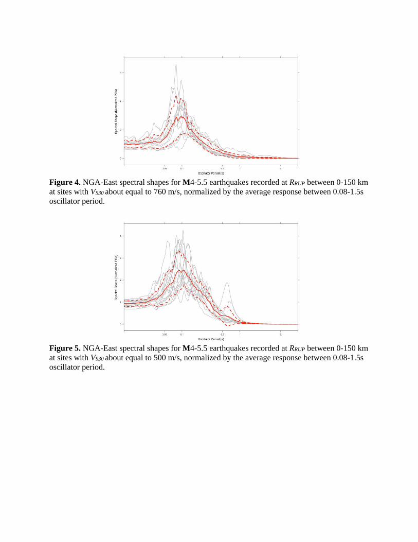
Figure 4. NGA-East spectral shapes for M4-5.5 earthquakes recorded at RRUP between 0-150 km at sites with VS30 about equal to 760 m/s, normalized by the average response between 0.08-1.5s oscillator period.

Figure 5. NGA-East spectral shapes for M4-5.5 earthquakes recorded at RRUP between 0-150 km at sites with VS30 about equal to 500 m/s, normalized by the average response between 0.08-1.5s oscillator period.

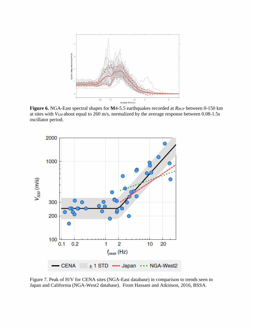
Figure 6. NGA-East spectral shapes for M4-5.5 earthquakes recorded at RRUP between 0-150 km at sites with VS30 about equal to 260 m/s, normalized by the average response between 0.08-1.5s oscillator period.

Figure 7. Peak of H/V for CENA sites (NGA-East database) in comparison to trends seen in Japan and California (NGA-West2 database). From Hassani and Atkinson, 2016, BSSA.

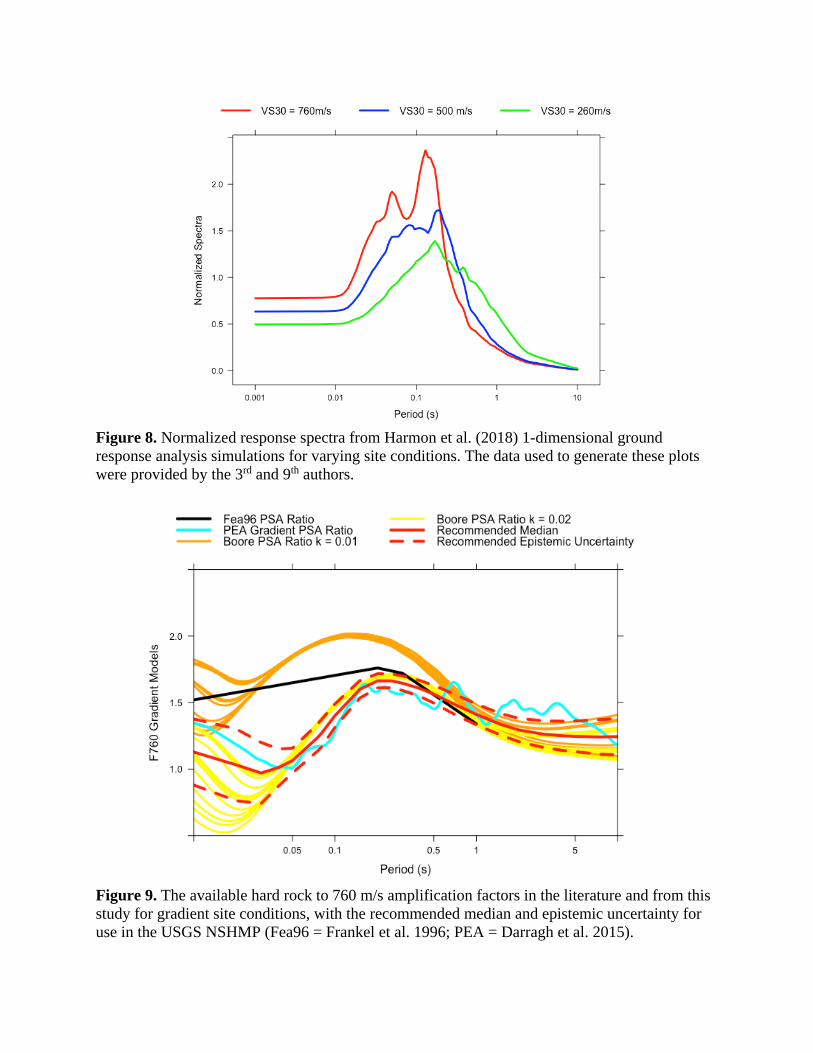
Figure 8. Normalized response spectra from Harmon et al. (2018) 1-dimensional ground response analysis simulations for varying site conditions. The data used to generate these plots were provided by the 3rd and 9th authors.

Figure 9. The available hard rock to 760 m/s amplification factors in the literature and from this study for gradient site conditions, with the recommended median and epistemic uncertainty for use in the USGS NSHMP (Fea96 = Frankel et al. 1996; PEA = Darragh et al. 2015).

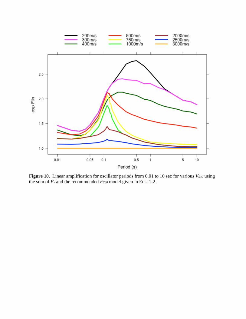
Figure 10. Linear amplification for oscillator periods from 0.01 to 10 sec for various VS30 using the sum of Fv and the recommended F760 model given in Eqs. 1-2.

Table 1. Tabulated values of the recommended median gradient F760 model and the associated epistemic uncertainty.

Period (s) Median Gradient F760 (LN Units)

Epistemic Uncertainty (LN Units)

PGV 0.297 0.117 PGA 0.121 0.248 0.01 0.121 0.248 0.02 0.031 0.270 0.03 0.000 0.229 0.04 0.012 0.139 0.05 0.062 0.093 0.075 0.211 0.102 0.08 0.237 0.103 0.1 0.338 0.088

0.15 0.470 0.066 0.2 0.509 0.053

0.25 0.509 0.052 0.3 0.498 0.055 0.4 0.473 0.060 0.5 0.447 0.067

0.75 0.386 0.077 0.8 0.378 0.077 1 0.344 0.078

1.5 0.289 0.081 2 0.258 0.088 3 0.233 0.100 4 0.224 0.109 5 0.220 0.115

7.5 0.216 0.130 10 0.218 0.137

Revision to Fnl term

Plots provided by Peter Powers showed that the nonlinear term (Fnl) was reducing site amplification values at 760 m/s at short periods. We do not expect nonlinearity for these conditions.

Accordingly, the 3rd and 8th authors have developed an adjustment to the Fnl model that

provides for essentially no nonlinearity at 760 m/s. In the report presenting this model originally (Hashash et al. 2017), the nonlinearity is quantified with term f2, as written in Eq. (2.3) of that

report. In the original recommended model, parameter Vref was set to 3000 m/s, which allows for some (although small) nonlinearity for 760 ≤ VS30 < Vref.

Our revised recommendation is to retain Vref = 3000 m/s for periods of 0.4 sec and

greater, but to change to Vref = 760 m/s for shorter periods (Eq. 3.3 in Hashash et al., 2017). This produces a step in the Fnl term at 0.4 sec, but it is sufficiently small as to be of negligible importance (Figure 11). Coefficients for the Fnl term at more closely spaced periods between 0.1-0.2s are given in Table 3.

Adjustment to the Fv term for fast sites

The 5th author found a problem with an earlier model revision that we had provided in the

form of Power Point file on 2/23/2018. This problem produced a discontinuity in amplification at 0.4 sec. We have made some adjustments to the V2 parameter and the model equations that correct the problem. The equation change is for the computation of Fv for sites with 2000 > VS30 > V2, for which the amplification is now computed as follows for all periods:

𝐹𝐹𝑣𝑣 = 𝑐𝑐 ∙ 𝑙𝑙𝑙𝑙 � 𝑉𝑉2𝑉𝑉𝑟𝑟𝑟𝑟𝑟𝑟

� : 2000 𝑚𝑚/𝑠𝑠 > 𝑉𝑉𝑆𝑆30 > 𝑉𝑉2 (3)

The revised coefficients for Fv are given in Table 2. Coefficients c and V1 were smoothed after revising V2, and are also given in Table 2. Lastly, values of the F760 impedance model and epistemic uncertainty are given in Table 2 at denser periods between 0.1-0.2s than reported in Sea17. This is in order to capture the peak of the model, which occurs around 0.117s. For velocities between 2000 and 3000 m/s, we interpolate Fv in a log-linear manner between the value of Fv for 2000 m/s and zero (at 3000 m/s) as follows:

𝐹𝐹𝑣𝑣 = −2.466𝐹𝐹𝑣𝑣(2000) ∙ 𝑙𝑙𝑙𝑙 �𝑉𝑉𝑆𝑆303000

� : 3000 > 𝑉𝑉𝑆𝑆30 > 2000 𝑚𝑚/𝑠𝑠 (4) The uncertainty in Fv, denoted σv, is given in Eq. (2.4) of Sea17 for sites up to 2000 m/s. For faster sites, σv can be taken as follows:

𝜎𝜎𝑣𝑣 = 𝜎𝜎𝑣𝑣(2000)�1 −𝑙𝑙𝑙𝑙�𝑉𝑉𝑆𝑆30 2000� �

𝑙𝑙𝑙𝑙�3000 2000� �� : 3000 > 𝑉𝑉𝑆𝑆30 > 2000 𝑚𝑚/𝑠𝑠 (5)

Table 2. Updated Fv model coefficients and F760 impedance model at additional periods to capture peak amplification.

Period (s) c V1 (m/s) V2 (m/s) Vref (m/s) F760 Impedance ( i )

F760 Impedance σ -1 -0.449 331 760 760 0.375 0.313 0 -0.290 319 760 760 0.185 0.434

0.01 -0.290 319 760 760 0.185 0.434 0.02 -0.303 319 760 760 0.185 0.434 0.03 -0.315 319 810 760 0.224 0.404 0.04 -0.331 319 900 760 0.283 0.390 0.05 -0.344 319 1010 760 0.337 0.363

0.075 -0.348 319 1380 760 0.475 0.322 0.08 -0.358 318 1450 760 0.512 0.335 0.1 -0.372 317 1900 760 0.674 0.366 0.11 -0.374 315 2000 760 0.730 0.352

0.112 -0.375 315 2000 760 0.741 0.348 0.113 -0.375 315 2000 760 0.747 0.345 0.114 -0.375 314 2000 760 0.753 0.343 0.115 -0.375 314 2000 760 0.758 0.340 0.116 -0.375 314 2000 760 0.761 0.338 0.117 -0.376 313 2000 760 0.762 0.335 0.118 -0.376 313 2000 760 0.761 0.333 0.119 -0.376 313 2000 760 0.759 0.330 0.12 -0.376 313 2000 760 0.756 0.327

0.125 -0.378 311 2000 760 0.732 0.313 0.13 -0.379 309 2000 760 0.716 0.299

0.135 -0.380 307 1800 760 0.669 0.286 0.14 -0.382 306 1775 760 0.660 0.273 0.15 -0.385 302 1500 760 0.586 0.253 0.2 -0.403 279 1073 760 0.419 0.214 0.25 -0.417 250 945 760 0.332 0.177 0.3 -0.426 225 867 760 0.270 0.131 0.4 -0.452 217 843 760 0.209 0.112 0.5 -0.480 217 822 760 0.175 0.105 0.75 -0.510 227 814 760 0.127 0.138 0.8 -0.523 235 810 760 0.120 0.133 1 -0.557 255 790 760 0.095 0.124

1.5 -0.574 276 805 760 0.083 0.112 2 -0.584 296 810 760 0.079 0.118 3 -0.588 312 820 760 0.073 0.111 4 -0.579 321 821 760 0.066 0.120 5 -0.558 324 825 760 0.064 0.108

7.5 -0.544 325 820 760 0.056 0.082 10 -0.507 325 820 760 0.053 0.069

Figure 11 (a) Adjusted (red) and previous (black) Fnl models for VS30 = 760 m/s and PGAr = 1.0 g. The blue arrow shows the boundary (T = 0.4 s) between adjusted and previous models to indicate that the step in the Fnl term at T = 0.4 s is negligible, (b) Adjusted Fnl term for various VS30 values and PGAr = 1.0 g to show that any unexpected step in Fnl term does not occur for sites of VS30 < 760 m/s subjected to strong shaking.

0.01 0.1 1 10Period (s)

0.2

0.4

0.6

0.8

1

1.2

VS30 (m/s)200300400

500600

700760

0.01 0.1 1 10Period (s)

0.4

0.6

0.8

1

1.2ex

p(F nl

)

Adjusted Fnl Previous Fnl

(a) (b)

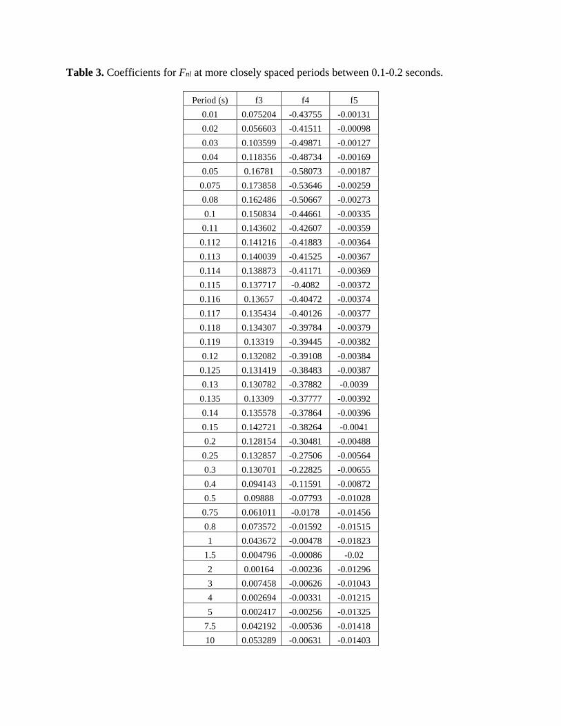
Table 3. Coefficients for Fnl at more closely spaced periods between 0.1-0.2 seconds.

Period (s) f3 f4 f5 0.01 0.075204 -0.43755 -0.00131 0.02 0.056603 -0.41511 -0.00098 0.03 0.103599 -0.49871 -0.00127 0.04 0.118356 -0.48734 -0.00169 0.05 0.16781 -0.58073 -0.00187 0.075 0.173858 -0.53646 -0.00259 0.08 0.162486 -0.50667 -0.00273 0.1 0.150834 -0.44661 -0.00335

0.11 0.143602 -0.42607 -0.00359 0.112 0.141216 -0.41883 -0.00364 0.113 0.140039 -0.41525 -0.00367 0.114 0.138873 -0.41171 -0.00369 0.115 0.137717 -0.4082 -0.00372 0.116 0.13657 -0.40472 -0.00374 0.117 0.135434 -0.40126 -0.00377 0.118 0.134307 -0.39784 -0.00379 0.119 0.13319 -0.39445 -0.00382 0.12 0.132082 -0.39108 -0.00384 0.125 0.131419 -0.38483 -0.00387 0.13 0.130782 -0.37882 -0.0039 0.135 0.13309 -0.37777 -0.00392 0.14 0.135578 -0.37864 -0.00396 0.15 0.142721 -0.38264 -0.0041 0.2 0.128154 -0.30481 -0.00488

0.25 0.132857 -0.27506 -0.00564 0.3 0.130701 -0.22825 -0.00655 0.4 0.094143 -0.11591 -0.00872 0.5 0.09888 -0.07793 -0.01028

0.75 0.061011 -0.0178 -0.01456 0.8 0.073572 -0.01592 -0.01515 1 0.043672 -0.00478 -0.01823

1.5 0.004796 -0.00086 -0.02 2 0.00164 -0.00236 -0.01296 3 0.007458 -0.00626 -0.01043 4 0.002694 -0.00331 -0.01215 5 0.002417 -0.00256 -0.01325

7.5 0.042192 -0.00536 -0.01418 10 0.053289 -0.00631 -0.01403