principles of ct: multislice ct* - journal of nuclear...

Principles of CT: Multislice CT*

Lee W. Goldman

Department of Radiation Therapy and Medical Physics, Hartford Hospital, Hartford, Connecticut

This article describes the principles and evolution of multislice CT(MSCT), including conceptual differences associated with slicedefinition, cone beam effects, helical pitch, and helical scantechnique. MSCT radiation dosimetry is described, and dose is-sues associated with MSCT—and with CT in general—as well astechniques for reducing patient radiation dose are discussed.Factors associated with the large volume of data associatedwith MSCT examinations are presented.

Key Words: CT; multislice CT; radiation dosimetry

J Nucl Med Technol 2008; 36:57–68DOI: 10.2967/jnmt.107.044826

This article, the third in a series of continuing educationarticles on the principles of CT, focuses on multislice CT(MSCT).

PRINCIPLES OF MSCT

Limitations of Single-Slice Slip Ring and HelicalScanners

Soon after their introduction in the late 1980s, slip ringscanners and helical (spiral) CT were rapidly adopted andsoon became the de facto standard of care for body CT.However, a significant problem became evident: helical CTwas very hard on x-ray tubes. For example, an abdomen–pelvis helical CT covering 60 cm (600 mm) of anatomywith a 5-mm slice thickness, a pitch of 1.0 (thus requiring120 rotations), and typical technique factors (120 kilovolts[peak] [kVp], 250 mA, 1-s rotation time) deposits a total of3.6 · 106 J of heat in the x-ray tube anode. Before slip ringCT, individual slices obtained with an equivalent technique(120 kVp, 250 mA, 1-s scan) would deposit only 30,000 J,much of which could be dissipated during the relativelylengthy (several seconds) interscan delay.

A limitation imposed by tube heating was that the thinslices (,3 mm) desired for acceptable-quality reformat-

ting into off-axis images (coronal, sagittal, or oblique) or3-dimensional reconstructions were impractical unless thescanned region was very limited or the scan technique wasseverely constrained. It was not uncommon for scanners tolimit a helical technique with thin slices to 100 mAs (tubecurrent in milliamperes · scan time in seconds) or less perrotation, yielding low-quality, noisy images.

A straightforward solution to this heat issue, of course, isto develop x-ray tubes with a higher heat capacity; suchtubes have been asnd continue to be developed. Anotherapproach is to more effectively use the available x-raybeam: if the x-ray beam is widened in the z-direction (slicethickness) and if multiple rows of detectors are used, thendata can be collected for more than one slice at a time. Thisapproach would reduce the total number of rotations—andtherefore the total usage of the x-ray tube—needed to coverthe desired anatomy. This is the basic idea of MSCT.

Although both third- and fourth-generation scannerswere in common use as single-slice scanners, all multislicescanners are based on a third-generation platform. There-fore, in the following discussion, third-generation scannergeometry (tube and detector bank linked and rotatingtogether) is assumed.

MSCT Detectors

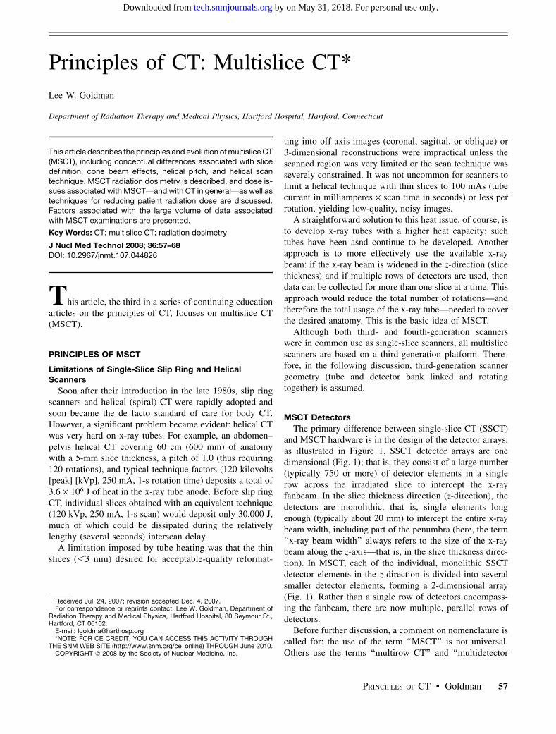
The primary difference between single-slice CT (SSCT)and MSCT hardware is in the design of the detector arrays,as illustrated in Figure 1. SSCT detector arrays are onedimensional (Fig. 1); that is, they consist of a large number(typically 750 or more) of detector elements in a singlerow across the irradiated slice to intercept the x-rayfanbeam. In the slice thickness direction (z-direction), thedetectors are monolithic, that is, single elements longenough (typically about 20 mm) to intercept the entire x-raybeam width, including part of the penumbra (here, the term‘‘x-ray beam width’’ always refers to the size of the x-raybeam along the z-axis—that is, in the slice thickness direc-tion). In MSCT, each of the individual, monolithic SSCTdetector elements in the z-direction is divided into severalsmaller detector elements, forming a 2-dimensional array(Fig. 1). Rather than a single row of detectors encompass-ing the fanbeam, there are now multiple, parallel rows ofdetectors.

Before further discussion, a comment on nomenclature iscalled for: the use of the term ‘‘MSCT’’ is not universal.Others use the terms ‘‘multirow CT’’ and ‘‘multidetector

Received Jul. 24, 2007; revision accepted Dec. 4, 2007.For correspondence or reprints contact: Lee W. Goldman, Department of

Radiation Therapy and Medical Physics, Hartford Hospital, 80 Seymour St.,Hartford, CT 06102.

E-mail: [email protected]*NOTE: FOR CE CREDIT, YOU CAN ACCESS THIS ACTIVITY THROUGH

THE SNM WEB SITE (http://www.snm.org/ce_online) THROUGH June 2010.COPYRIGHT ª 2008 by the Society of Nuclear Medicine, Inc.

PRINCIPLES OF CT • Goldman 57

by on May 31, 2018. For personal use only. tech.snmjournals.org Downloaded from

http://tech.snmjournals.org/

row CT (MDCT)’’ because they are more descriptive of thistechnology than the term ‘‘multislice CT.’’ Throughout thisarticle, however, the term ‘‘MSCT’’ is used.

The first scanner with more than one row of detectorsand a widened z-axis x-ray beam was introduced by Elscintin 1992 (CT-Twin). This scanner had 2 rows of detectors,allowing data for 2 slices to be acquired simultaneously,and was developed primarily to help address the x-ray tubeheating problem. As a curious historical note, according tothe description given earlier in this article, the first MSCTscanner would actually be the first-generation EMI Mark 1.With 2 adjacent detectors and a widened x-ray beam, thisscanner collected data for 2 slices at the same time andthereby reduced the lengthy examination time associatedwith the 5- to 6-min scan time (1). The first scanners of the‘‘modern MSCT era’’ were introduced in late 1998 and aredescribed in the following discussion (1).

MSCT Data Acquisition

A detector design used in one of the first modern MSCTscanners (Fig. 1) consisted of 16 rows of detector elements,each 1.25 mm long in the z-direction, for a total z-axislength of 20 mm. Each of the 16 detector rows could, inprinciple, simultaneously collect data for 16 slices, each1.25 mm thick; however, this approach would require han-dling an enormous amount of data very quickly, because atypical scanner may acquire 1,000 views per rotation. Ifthere are 800 detectors per row and 16 rows, then almost 13million measurements must be made during a single rota-tion with a duration of as short as 0.5 s.

Because of the initial limitations in acquiring and handlingsuch large amounts of data, the first versions of modernMSCT scanners limited simultaneous data acquisition to 4

slices. Four detector ‘‘rows’’ corresponding to the 4 simul-taneously collected slices fed data into 4 parallel data‘‘channels,’’ so that these 4-slice scanners were said to pos-sess 4 data channels. These 4-slice scanners, however, werequite flexible with regard to how detector rows could beconfigured; groups of detector elements in the z-directioncould be electronically linked to function as a single, longerdetector, thus providing much flexibility in the slice thick-ness of the 4 acquired slices. Examples of detector config-urations used with the 4 channels are illustrated in Figure 2for 2 versions of 4-slice MSCT detectors: one based on thedetector design described earlier (16 rows of 1.25-mm ele-ments) and the other based on an ‘‘adaptive array’’ consistingof detector elements of different sizes (other detector designswere used by other manufacturers) (2,3).

Possible detector configurations for the detector designencompassing 16 rows of 1.25-mm elements for the acqui-sition of 4 slices are illustrated in Figures 2A and 2B. InFigure 2A, 4 elements in a group are linked to act as asingle 5-mm detector (4 · 1.25). The result is four 5-mmdetectors covering a total z-axis length of 20 mm. When a20-mm-wide x-ray beam is used, 4 slices with a thicknessof 5 mm are acquired. The acquired 5-mm slices can alsobe combined into 10-mm slices, if desired. In Figure 2B,4 pairs of detector elements are linked to function as four2.5-mm detectors (2 · 1.25). When a 10-mm-wide x-raybeam is used, four 2.5-mm slices can be acquired simul-taneously. Again, the resulting 2.5-mm slices can be com-bined to form 5-mm slices (5-mm axial slices are generallypreferred for interpretation purposes). A third possibility isto use a 5-mm-wide x-ray beam to irradiate only the 4innermost individual detector elements for the acquisitionof four 1.25-mm slices. Yet another possibility is to link

FIGURE 1. (Left) SSCT arrays contain-ing single, long elements along z-axis.(Right) MSCT arrays with several rows ofsmall detector elements.

58 JOURNAL OF NUCLEAR MEDICINE TECHNOLOGY • Vol. 36 • No. 2 • June 2008



elements in triplets and use a 15-mm-wide x-ray beam toacquire four 3.75-mm slices.

Similarly, the individual elements of the adaptive arraycan be appropriately linked to acquire four 5-mm slices(Fig. 2C) or four 2.5-mm slices (Fig. 2D). Another possi-bility is to use a 4-mm-wide x-ray beam (which wouldirradiate only part of the 1.5-mm elements) to yield four1-mm slices. Thinner slices can be combined to formthicker slices for interpretation purposes, if necessary.

As data acquisition technology advanced, more datachannels were provided to allow the simultaneous acquisi-tion of more than 4 slices. An 8-channel version of thesystem encompassing the detector array in Figures 2A and2B (introduced approximately 3 y later) could acquire eight2.5-mm slices or eight 1.25-mm slices (which could becombined to form thicker slices for interpretation).

Submillimeter Slices and Isotropic Resolution

The 4-slice and 8-slice MSCT scanners just describedwere also capable of acquiring ultrathin (‘‘submillimeter’’)slices (but only 2 at a time) by collimating the x-ray beamin the z-axis to partially irradiate the 2 innermost detectorelements in the detector array. For example, for the detectorarray in Figure 2A, if the x-ray beam is collimated to a1.25-mm width and aligned so as to straddle and partiallyirradiate the 2 innermost detector elements, then 2 slices,each 0.625 mm thick, can be obtained. When imagesresulting from such an acquisition are reformatted intosagittal, coronal, or other off-axis images, the reformattedimages exhibit spatial resolution in the z-direction that isessentially equal to that within the plane of the axial slices.Resolution that is (essentially) equal in all 3 directions issaid to be isotropic.

Because only 2 submillimeter slices could be acquiredsimultaneously with these earlier MSCT scanners, thiscapability was not widely used because of limited z-axis

coverage and tube heating limitations. Submillimeter scan-ning had to await the introduction of 16-slice scanners.

16-Channel (16-Slice) Scanners—and More

The installation of MSCT scanners providing 16 datachannels for 16 simultaneously acquired slices began in2002. In addition to simultaneously acquiring up to 16slices, the detector arrays associated with 16-slice scannerswere redesigned to allow thinner slices to be obtained aswell. Detector arrays for various 16-slice scanner modelsare illustrated in Figure 3. Note that in all of the models, theinnermost 16 detector elements along the z-axis are half thesize of the outermost elements, allowing the simultaneousacquisition of 16 thin slices (from 0.5 mm thick to 0.75 mmthick, depending on the model). When the inner detectorswere used to acquire submillimeter slices, the total acquiredz-axis length and therefore the total width of the x-ray beamranged from 8 mm for the Toshiba version to 12 mm for thePhilips and Siemens versions. Alternatively, the inner 16

FIGURE 2. Flexible use of detectors in4-slice MSCT scanners. (A) Groups offour 1.25-mm-wide elements are linkedto act as 5-mm-wide detectors. (B) Inner8 elements are linked in pairs to act as2.5-mm detectors. (C) Inner, adaptive-array elements are linked to act as 5-mmdetectors (1 1 1.5 1 2.5) and, togetherwith outer, 5-mm elements, yield four5-mm slices. (D) The 4 innermost ele-ments are linked in pairs to form 2.5-mmdetectors (1 1 1.5), which along with thetwo 2.5-mm detectors, collect data forfour 2.5-mm slices.

FIGURE 3. Diagrams of various 16-slice detector designs (inz-direction). Innermost elements can be used to collect 16 thinslices or linked in pairs to collect thicker slices.




elements could be linked in pairs for the acquisition of 16thicker slices (4).

During 2003 and 2004, MSCT manufacturers introducedmodels with both fewer than and more than 16 channels.Six-slice and 8-slice models were introduced by manufac-turers as cost-effective alternatives. At the same time,32-slice and 40-slice scanners were being introduced.

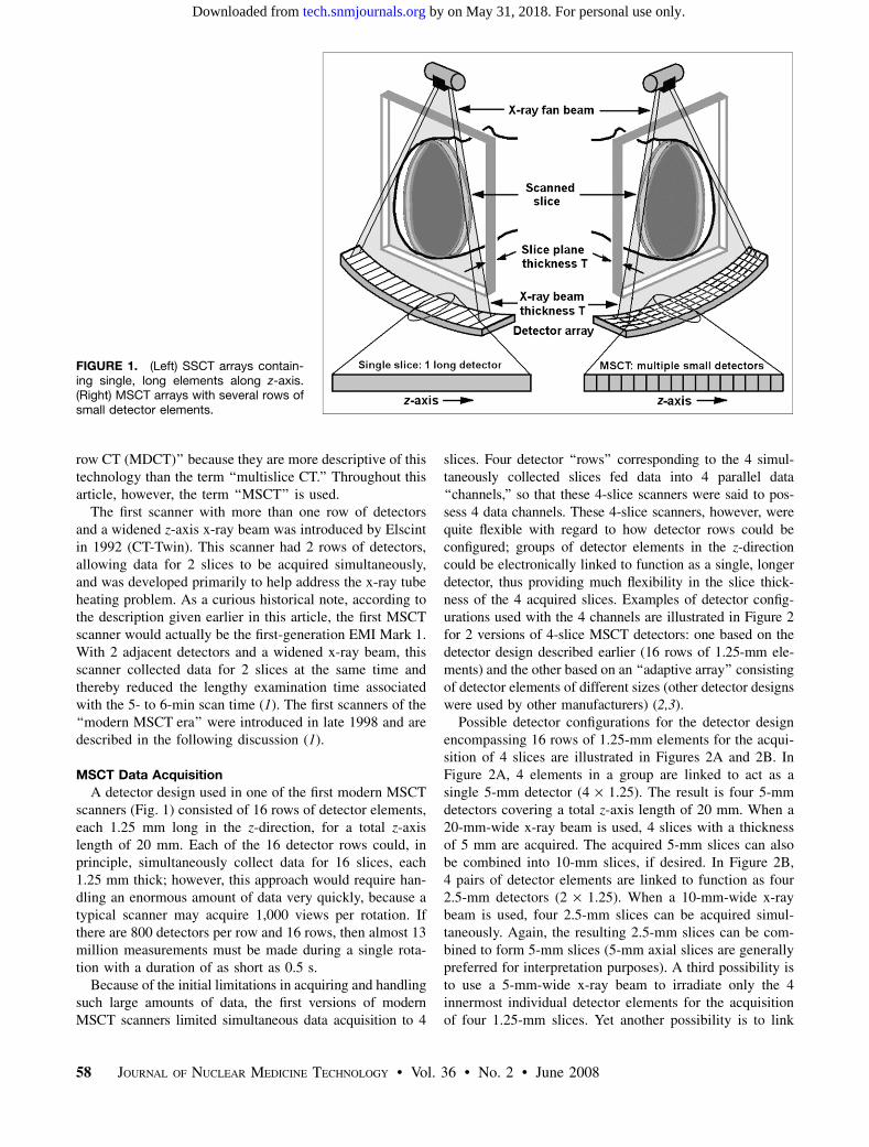
By 2005, 64-slice scanners were announced, and instal-lations by most manufacturers began. Detector array de-signs used by several manufacturers are illustrated in Figure4. The approach used by most manufacturers for 64-slicedetector array designs was to lengthen the arrays in thez-direction and provide all submillimeter detector elements:64 · 0.625 mm (total z-axis length of 40 mm) for thePhilips and GE Healthcare models and 64 · 0.5 mm (totalz-axis length of 32 mm) for the Toshiba model. The designapproach of Siemens was quite different. The detector arrayof the Siemens 32-slice scanner (containing 32 elementseach 0.6 mm long, for a total z-axis length of 19.2 mm) wascombined with a ‘‘dynamic-focus’’ x-ray tube for thesimultaneous acquisition of 64 slices. This x-ray tube couldelectronically—and very quickly—shift the focal spot lo-cation on the x-ray tube target so as to emit radiation from aslightly different position along the z-axis. Each of the 32detector elements then collected 2 measurements (samples),separated along the z-axis by approximately 0.3 mm. The netresult was a total of 64 measurements (32 detectors · 2measurements per detector) along a 19.2-mm total z-axisfield of view (this process is referred to in Siemensliterature as ‘‘Z-Sharp’’ technology) (5).

In the preceding examples, in addition to the simulta-neous acquisition of more slices, MSCT x-ray beam widthscan be considerably wider than those for SSCT. Sixteen-slice MSCT beam widths are up to 32 mm; 64-slice beamscan be up to 40 mm wide; and even wider beams are used insystems currently under development or in clinical evalu-ation. A possible consequence is that more scatter mayreach the detectors, compromising low-contrast detection.Generally, however, the antiscatter septa traditionally used

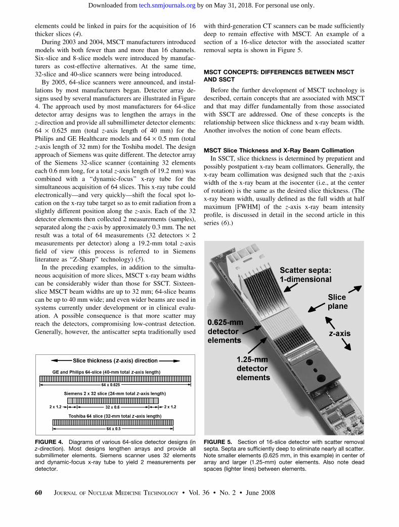
with third-generation CT scanners can be made sufficientlydeep to remain effective with MSCT. An example of asection of a 16-slice detector with the associated scatterremoval septa is shown in Figure 5.

MSCT CONCEPTS: DIFFERENCES BETWEEN MSCTAND SSCT

Before the further development of MSCT technology isdescribed, certain concepts that are associated with MSCTand that may differ fundamentally from those associatedwith SSCT are addressed. One of these concepts is therelationship between slice thickness and x-ray beam width.Another involves the notion of cone beam effects.

MSCT Slice Thickness and X-Ray Beam Collimation

In SSCT, slice thickness is determined by prepatient andpossibly postpatient x-ray beam collimators. Generally, thex-ray beam collimation was designed such that the z-axiswidth of the x-ray beam at the isocenter (i.e., at the centerof rotation) is the same as the desired slice thickness. (Thex-ray beam width, usually defined as the full width at halfmaximum [FWHM] of the z-axis x-ray beam intensityprofile, is discussed in detail in the second article in thisseries (6).)

FIGURE 4. Diagrams of various 64-slice detector designs (inz-direction). Most designs lengthen arrays and provide allsubmillimeter elements. Siemens scanner uses 32 elementsand dynamic-focus x-ray tube to yield 2 measurements perdetector.

FIGURE 5. Section of 16-slice detector with scatter removalsepta. Septa are sufficiently deep to eliminate nearly all scatter.Note smaller elements (0.625 mm, in this example) in center ofarray and larger (1.25-mm) outer elements. Also note deadspaces (lighter lines) between elements.




In MSCT, however, slice thickness is determined bydetector configuration and not x-ray beam collimation. Forexample, the 4 slices in Figure 2A are each 5 mm thickbecause they are acquired by 5-mm detectors (formed bylinking four 1.25-mm detector elements). The 4 slices inFigure 2B are 2.5 mm thick because they are acquired by2.5-mm detectors (formed by linking two 1.25-mm ele-ments). Because it is the length of the individual detector(or linked detector elements) acquiring data for each of thesimultaneously acquired slices that limits the width of thex-ray beam contributing to that slice, this length is oftenreferred to as detector collimation. In Figures 2A and 2C,the detector collimation is 5 mm. In Figures 2B and 2D, thedetector collimation is 2.5 mm. The actual x-ray beamcollimation is not directly involved in determining slicethickness, other than that the ‘‘total’’ z-axis beam collima-tion should be equal to the total thickness of the 4 slices, forexample, 20 mm in Figure 2A or 10 mm in Figure 2B (thatthis is not necessarily true is discussed in the MSCTdosimetry section later in this article) (7).

Cone Beam Effects in MSCT

Cone beam effects in CT are associated with the diver-gent nature of the x-ray beam emitted from the x-ray tube.This divergence means that the z-axis of the x-ray beam issomewhat wider when it exits the patient than when itentered the patient.

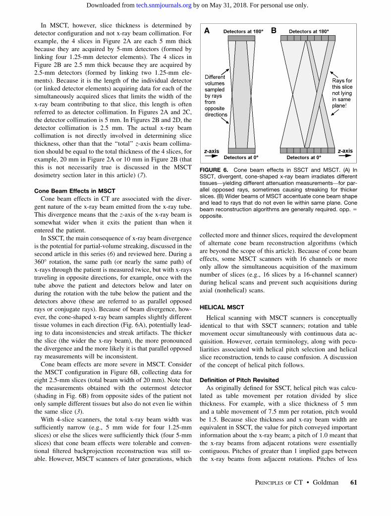
In SSCT, the main consequence of x-ray beam divergenceis the potential for partial-volume streaking, discussed in thesecond article in this series (6) and reviewed here. During a360� rotation, the same path (or nearly the same path) ofx-rays through the patient is measured twice, but with x-raystraveling in opposite directions, for example, once with thetube above the patient and detectors below and later onduring the rotation with the tube below the patient and thedetectors above (these are referred to as parallel opposedrays or conjugate rays). Because of beam divergence, how-ever, the cone-shaped x-ray beam samples slightly differenttissue volumes in each direction (Fig. 6A), potentially lead-ing to data inconsistencies and streak artifacts. The thickerthe slice (the wider the x-ray beam), the more pronouncedthe divergence and the more likely it is that parallel opposedray measurements will be inconsistent.

Cone beam effects are more severe in MSCT. Considerthe MSCT configuration in Figure 6B, collecting data foreight 2.5-mm slices (total beam width of 20 mm). Note thatthe measurements obtained with the outermost detector(shading in Fig. 6B) from opposite sides of the patient notonly sample different tissues but also do not even lie withinthe same slice (3).

With 4-slice scanners, the total x-ray beam width wassufficiently narrow (e.g., 5 mm wide for four 1.25-mmslices) or else the slices were sufficiently thick (four 5-mmslices) that cone beam effects were tolerable and conven-tional filtered backprojection reconstruction was still us-able. However, MSCT scanners of later generations, which

collected more and thinner slices, required the developmentof alternate cone beam reconstruction algorithms (whichare beyond the scope of this article). Because of cone beameffects, some MSCT scanners with 16 channels or moreonly allow the simultaneous acquisition of the maximumnumber of slices (e.g., 16 slices by a 16-channel scanner)during helical scans and prevent such acquisitions duringaxial (nonhelical) scans.

HELICAL MSCT

Helical scanning with MSCT scanners is conceptuallyidentical to that with SSCT scanners; rotation and tablemovement occur simultaneously with continuous data ac-quisition. However, certain terminology, along with pecu-liarities associated with helical pitch selection and helicalslice reconstruction, tends to cause confusion. A discussionof the concept of helical pitch follows.

Definition of Pitch Revisited

As originally defined for SSCT, helical pitch was calcu-lated as table movement per rotation divided by slicethickness. For example, with a slice thickness of 5 mmand a table movement of 7.5 mm per rotation, pitch wouldbe 1.5. Because slice thickness and x-ray beam width areequivalent in SSCT, the value for pitch conveyed importantinformation about the x-ray beam; a pitch of 1.0 meant thatthe x-ray beams from adjacent rotations were essentiallycontiguous. Pitches of greater than 1 implied gaps betweenthe x-ray beams from adjacent rotations. Pitches of less

FIGURE 6. Cone beam effects in SSCT and MSCT. (A) InSSCT, divergent, cone-shaped x-ray beam irradiates differenttissues—yielding different attenuation measurements—for par-allel opposed rays, sometimes causing streaking for thickerslices. (B) Wider beams of MSCT accentuate cone beam shapeand lead to rays that do not even lie within same plane. Conebeam reconstruction algorithms are generally required. opp. 5

opposite.




than 1 implied x-ray beam overlap (and thus doubleirradiation of some tissue) and so were not clinically used.

Applying this definition to MSCT creates confusion andtends to obscure important information. For example, a4-slice MSCT helical scan with 15 mm of table movementper rotation and a 20-mm-wide x-ray beam (to acquire four5-mm slices) would yield the following pitch calculationbased on the earlier definition: pitch 5 table movementper rotation/slice thickness 5 15 mm/5 mm 5 3.0. Thiscalculation does not immediately convey the fact thatalthough the pitch is much greater than 1, there is clearlyx-ray beam overlap, because the total width of the x-raybeam is 20 mm and the table is moving only 15 mm perrotation. To address this situation, a new definition of pitchwas adopted. In this definition, the denominator is replacedwith the total thickness of all of the simultaneously acquiredslices; that is, if n slices each of slice thickness T areacquired, then the total width is n · T, and the new pitchdefinition is as follows: pitch 5 table movement per rotation/(n · T) (beam pitch). Because the original definition is stilloccasionally referenced, the new pitch definition in the latterequation is called ‘‘beam pitch.’’ The original definition isnow referred to as ‘‘detector pitch,’’ on the basis of the ideathat slice thickness (in the denominator of the originaldefinition) in MSCT is determined by detector configuration.With the new definition, beam pitch for the example justgiven would be calculated as follows: pitch 5 table move-ment per rotation/(n · T) 5 15 mm/(4 · 5 mm) 5 0.75.Because beam pitch conveys similar information for MSCTas the original definition did for SSCT, it is the preferreddefinition in most situations (2).

Pitch and z Sampling in Helical MSCT

Clinical pitch selection in SSCT was generally straight-forward. Typically, only 2 pitches were commonly used:pitch 5 1 for best quality and pitch 5 1.5 when more z-axiscoverage was needed in a shorter time (because of eithertotal scan time or x-ray tube heating constraints). Pitches ofless than 1 were not used. In contrast, commonly used beampitches in MSCT may seem odd (e.g., 0.9375, 1.125, or1.375) and are very often less than 1. Before helical pitch inMSCT is discussed, the basic trade-off involving pitchselection is reviewed (see the first article in this series (8)for a more complete discussion).

Because of continuous table movement, no specific sliceposition along the z-axis actually contains sufficient data(i.e., transmission measurements along ray paths throughthe slice at sufficient locations and angles) to reconstruct animage. Rather, required measurements are estimated byinterpolation between the nearest measurements above andbelow the slice plane that are at the same relative positionand angle. The distance along the z-axis between thesemeasurements that is available for interpolation is referredto here as the z-spacing. Interpolated data may be inaccu-rate if anatomy changes significantly within the z-spacing,leading to streak or shading artifacts. Helical interpolation

artifacts often appear as (and are referred to as) ‘‘windmill’’artifacts, because when the helical images are pagedthrough quickly, the streak or shading artifacts seem torotate like the vanes of a windmill. The likelihood andseverity of helical artifacts increase with increasing z-spacing,because anatomy is more likely to change abruptly overdistance. Increasing pitch (to reduce either scan time orx-ray tube heating) increases distance between interpolatedmeasurements, so that the likelihood of helical artifactsincreases.

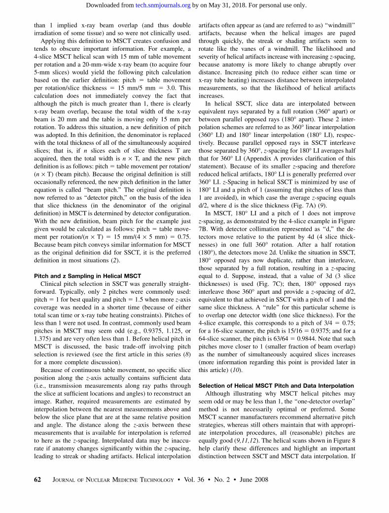
In helical SSCT, slice data are interpolated betweenequivalent rays separated by a full rotation (360� apart) orbetween parallel opposed rays (180� apart). These 2 inter-polation schemes are referred to as 360� linear interpolation(360� LI) and 180� linear interpolation (180� LI), respec-tively. Because parallel opposed rays in SSCT interleavethose separated by 360�, z-spacing for 180� LI averages halfthat for 360� LI (Appendix A provides clarification of thisstatement). Because of its smaller z-spacing and thereforereduced helical artifacts, 180� LI is generally preferred over360� LI. z-Spacing in helical SSCT is minimized by use of180� LI and a pitch of 1 (assuming that pitches of less than1 are avoided), in which case the average z-spacing equalsd/2, where d is the slice thickness (Fig. 7A) (9).

In MSCT, 180� LI and a pitch of 1 does not improvez-spacing, as demonstrated by the 4-slice example in Figure7B. With detector collimation represented as ‘‘d,’’ the de-tectors move relative to the patient by 4d (4 slice thick-nesses) in one full 360� rotation. After a half rotation(180�), the detectors move 2d. Unlike the situation in SSCT,180� opposed rays now duplicate, rather than interleave,those separated by a full rotation, resulting in a z-spacingequal to d. Suppose, instead, that a value of 3d (3 slicethicknesses) is used (Fig. 7C); then, 180� opposed raysinterleave those 360� apart and provide a z-spacing of d/2,equivalent to that achieved in SSCT with a pitch of 1 and thesame slice thickness. A ‘‘rule’’ for this particular scheme isto overlap one detector width (one slice thickness). For the4-slice example, this corresponds to a pitch of 3/4 5 0.75;for a 16-slice scanner, the pitch is 15/16 5 0.9375; and for a64-slice scanner, the pitch is 63/64 5 0.9844. Note that suchpitches move closer to 1 (smaller fraction of beam overlap)as the number of simultaneously acquired slices increases(more information regarding this point is provided later inthis article) (10).

Selection of Helical MSCT Pitch and Data Interpolation

Although illustrating why MSCT helical pitches mayseem odd or may be less than 1, the ‘‘one-detector overlap’’method is not necessarily optimal or preferred. SomeMSCT scanner manufacturers recommend alternative pitchstrategies, whereas still others maintain that with appropri-ate interpolation procedures, all (reasonable) pitches areequally good (9,11,12). The helical scans shown in Figure 8help clarify these differences and highlight an importantdistinction between SSCT and MSCT data interpolation. If




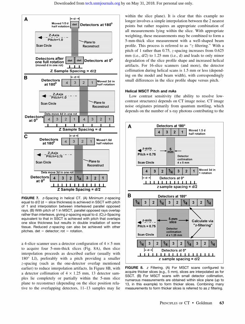
a 4-slice scanner uses a detector configuration of 4 · 5 mmto acquire four 5-mm-thick slices (Fig. 8A), then sliceinterpolation proceeds as described earlier (usually with180� LI), preferably with a pitch providing a smallerz-spacing (such as the one-detector overlap mentionedearlier) to reduce interpolation artifacts. In Figure 8B, witha detector collimation of 4 · 1.25 mm, 13 detector sam-ples lie completely or partially within the 5-mm sliceplane to reconstruct (depending on the slice position rela-tive to the overlapping detectors, 11–13 samples may lie

within the slice plane). It is clear that this example nolonger involves a simple interpolation between the 2 nearestpoints but rather requires an appropriate combination ofall measurements lying within the slice. With appropriateweighting, these measurements may be combined to form a5-mm-thick slice measurement with a well-shaped beamprofile. This process is referred to as ‘‘z filtering.’’ With apitch of 1 rather than 0.75, z-spacing increases from 0.625mm (i.e., d/2) to 1.25 mm (i.e., d) and leads to only minordegradation of the slice profile shape and increased helicalartifacts. For 16-slice scanners (and more), the detectorcollimation during helical scans is 1.5 mm or less (depend-ing on the model and beam width), with correspondinglysmall differences in the slice profile shape versus pitch.

Helical MSCT Pitch and mAs

Low contrast sensitivity (the ability to resolve low-contrast structures) depends on CT image noise. CT imagenoise originates primarily from quantum mottling, whichdepends on the number of x-ray photons contributing to the

FIGURE 7. z-Spacing in helical CT. (A) Minimum z-spacingequal to d/2 (d 5 slice thickness) is achieved in SSCT with pitchof 1 and interpolation between interleaved parallel opposedrays. (B) With pitch of 1 in MSCT, parallel opposed rays overlaprather than interleave, giving z-spacing equal to d. (C) z-Spacingequivalent to that in SSCT is achieved with pitch that overlapsone slice thickness but results in double irradiation of sometissue. Reduced z-spacing can also be achieved with otherpitches. det 5 detector; rot 5 rotation.

FIGURE 8. z Filtering. (A) For MSCT scans configured toacquire thicker slices (e.g., 5 mm), slices are interpolated as forSSCT. (B) For MSCT scans with small detector collimation,numerous measurements are obtained within slice plane (up to13, in this example) to form thicker slices. Combining manymeasurements to form thicker slices is referred to as z filtering.




image (the appearance of image noise also depends on thesharpness of the reconstruction filter used). To understandhow various factors affect CT image noise, it is easiest toconsider how many x-ray photons contribute to eachdetector measurement. Relevant factors include kVp (withhigher kVp, more x-rays penetrate the patient to reach thedetectors), slice thickness (the detectors collect more pho-tons over thicker slices), x-ray tube mA (a higher x-rayintensity increases the number of detected x-rays propor-tionally), and rotation time (faster rotation corresponds toshorter detector sampling times). The last 2 factors areoften taken together as mAs (see the second article in thisseries (6) for a more complete discussion).

Helical SSCT slices are reconstructed from data inter-polated between the 2 nearest parallel ray measurements(usually with 180� LI). Therefore, the number of x-rayphotons contributing to each interpolated sample (andtherefore to reducing image noise) is a linear combinationof 2 detector measurements, regardless of pitch. That is,helical SSCT image noise is unaffected by pitch (9). (Note,however, that the interpolation algorithm does affect imagenoise; fewer rays contribute to images when 180� LI is usedthan when 360� LI is used, so that 180� LI images aresomewhat noisier). Pitch does affect image noise in helicalMSCT if slice measurements are formed from manydetector samples. For example, the 5-mm slice in Figure8B is formed from a combination of 11–13 detector mea-surements. If the average x-ray flux reaching each detectorelement is n, then the number of x-ray photons contributingto the calculated (z-filtered) sample is between 11n and 13n.In comparison, a pitch of 1.5 and a detector collimation of4 · 1.25 mm results in only 5–7 detector measurementslying within the 5-mm slice plane and thus contributing toeach slice sample. For the same average detector flux n asthat used in the earlier example, the number of contributingx-ray photons is 5n–7n. That is, fewer x-ray photons con-tribute to each calculated slice sample for larger pitches,leading to noisier images.

In general, the number of photons contributing to imagesdecreases linearly with helical MSCT pitch if the samex-ray technique settings (kVp and mAs) are used. Asdiscussed later in this article, with the same x-ray techniquefactors, patient radiation dose (CT volume dose index[CTDIvol]) also decreases linearly with pitch (in effect,the same amount of energy is spread over more tissue inthe z-direction). Therefore, a practice adopted by somemanufacturers is to specify ‘‘effective’’mAs(mAseff), cal-culated as

mAseff 5 mAs=pitch;

rather than actual mAs, during examination prescription.mAseff is chosen to maintain the same level of image noiseregardless of selected pitch. For example, with 1-s rotationtimes, a mAseff of 240 uses 240 mA with a pitch of

1 (mAseff 5 240/1 5 240) but uses 300 mA with a pitchof 1.25 (mAseff 5 300/1.25) and 200 mA with a pitch of0.83 (mAseff 5 200/0.83).

MSCT RADIATION DOSIMETRY

Although axial and helical MSCT involves a morecomplex data collection process, measuring and specifyingpatient radiation doses in MSCT are no different from inSSCT. For both axial and helical dosimetry purposes,detector collimation is ignored and an MSCT scanner istreated as a single-slice scanner with a slice thickness equalto the full collimated x-ray beam width. For example, anMSCT scan with a detector collimation of 4 · 2.5 mm (totalbeam width of 10 mm) would be treated for dosimetrypurposes as an SSCT scan with a slice thickness of 10 mm(see the second article in this series (6) for a complete dis-cussion of CT dosimetry). For axial scans, therefore, theweighted CTDI [CTDIw] for a detector collimation of 4 ·2.5 mm (the slices from which may be combined to form10-mm slices) is equivalent in principle to that of a 10-mmSSCT slice. Similarly, the CTDIvol for helical scans is ob-tained from axial CTDIw measurements at the same beamcollimation by dividing the axial CTDIw by the pitch.

There are, however, certain factors that reduce the doseefficiency of MSCT relative to SSCT. In addition, certainMSCT practices that were uncommon or nonexistent inSSCT may lead to increased patient radiation doses. Thesefactors and issues are described in the following discussion.

MSCT Dose Efficiency

Dose efficiency refers to the fraction of x-rays that reachthe detectors and that are actually captured and contributeto image formation. Dose efficiency has 2 components:geometric efficiency and absorption efficiency. Absorptionefficiency refers to the fraction of x-rays that enter activedetector areas and that are actually absorbed (captured).Absorption efficiencies are similar for all SSCT and MSCTscanners that have solid-state detectors. Geometric effi-ciency refers to the fraction of x-rays that exit the patientand that enter active detector areas.

Two aspects of MSCT reduce its geometric dose effi-ciency relative to that of SSCT. The first is the obviousnecessity for dividers between individual detector elementsalong the z-axis, which create dead space that did not existwithin SSCT detectors in the z-direction (there is, of course,dead space from detector dividers within the slice plane forboth SSCT and MSCT). These dividers are visible in Figure5 as the thin, lighter lines between the small detectorelements. Depending on detector design and element size,dead space associated with the dividers can represent up to20% of the detector surface area. That is, up to 20% ofx-rays exiting the patient will strike dead space and notcontribute to image formation. Because these dividers mustsatisfy anti–cross talk and physical separation require-ments, divider width generally remains unchanged as de-tector elements are made smaller (compare the dividers




between the 0.625-mm elements and the 1.25-mm elementsin Fig. 5). Therefore, the dividers represent a larger fractionof detector surface area for smaller elements, leading tolower geometric efficiency. Reducing detector elementwidth from 1.25 mm to 0.635 mm or from 1.5 mm to0.75 mm approximately doubles the amount of dead space.Geometric efficiency loss is fixed by MSCT detector designand cannot be recovered (7).

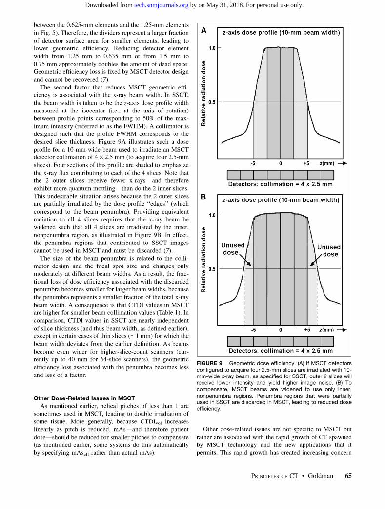
The second factor that reduces MSCT geometric effi-ciency is associated with the x-ray beam width. In SSCT,the beam width is taken to be the z-axis dose profile widthmeasured at the isocenter (i.e., at the axis of rotation)between profile points corresponding to 50% of the max-imum intensity (referred to as the FWHM). A collimator isdesigned such that the profile FWHM corresponds to thedesired slice thickness. Figure 9A illustrates such a doseprofile for a 10-mm-wide beam used to irradiate an MSCTdetector collimation of 4 · 2.5 mm (to acquire four 2.5-mmslices). Four sections of this profile are shaded to emphasizethe x-ray flux contributing to each of the 4 slices. Note thatthe 2 outer slices receive fewer x-rays—and thereforeexhibit more quantum mottling—than do the 2 inner slices.This undesirable situation arises because the 2 outer slicesare partially irradiated by the dose profile ‘‘edges’’ (whichcorrespond to the beam penumbra). Providing equivalentradiation to all 4 slices requires that the x-ray beam bewidened such that all 4 slices are irradiated by the inner,nonpenumbra region, as illustrated in Figure 9B. In effect,the penumbra regions that contributed to SSCT imagescannot be used in MSCT and must be discarded (7).

The size of the beam penumbra is related to the colli-mator design and the focal spot size and changes onlymoderately at different beam widths. As a result, the frac-tional loss of dose efficiency associated with the discardedpenumbra becomes smaller for larger beam widths, becausethe penumbra represents a smaller fraction of the total x-raybeam width. A consequence is that CTDI values in MSCTare higher for smaller beam collimation values (Table 1). Incomparison, CTDI values in SSCT are nearly independentof slice thickness (and thus beam width, as defined earlier),except in certain cases of thin slices (;1 mm) for which thebeam width deviates from the earlier definition. As beamsbecome even wider for higher-slice-count scanners (cur-rently up to 40 mm for 64-slice scanners), the geometricefficiency loss associated with the penumbra becomes lessand less of a factor.

Other Dose-Related Issues in MSCT

As mentioned earlier, helical pitches of less than 1 aresometimes used in MSCT, leading to double irradiation ofsome tissue. More generally, because CTDIvol increaseslinearly as pitch is reduced, mAs—and therefore patientdose—should be reduced for smaller pitches to compensate(as mentioned earlier, some systems do this automaticallyby specifying mAseff rather than actual mAs).

Other dose-related issues are not specific to MSCT butrather are associated with the rapid growth of CT spawnedby MSCT technology and the new applications that itpermits. This rapid growth has created increasing concern

FIGURE 9. Geometric dose efficiency. (A) If MSCT detectorsconfigured to acquire four 2.5-mm slices are irradiated with 10-mm-wide x-ray beam, as specified for SSCT, outer 2 slices willreceive lower intensity and yield higher image noise. (B) Tocompensate, MSCT beams are widened to use only inner,nonpenumbra regions. Penumbra regions that were partiallyused in SSCT are discarded in MSCT, leading to reduced doseefficiency.




about population exposure from CT. Rather than a detaileddescription of these issues, a brief list of some operationalpractices to help minimize patient radiation dose is pro-vided here; some of these were described in more detail inthe second article in this series (6).

Patient Size and Technique Selection. With the same scantechnique factors (kVp, mA, rotation time, and slice thick-ness), patient radiation dose (CTDI) is considerably higherfor smaller patients (13,14). For example, CTDIw measuredin the standard 16-cm dosimetry phantom (representing asmall pediatric patient) is nearly double that measured inthe standard 32-cm dosimetry phantom (representing amedium to large patient) with the same technique factors.It is important to adjust mAs appropriately for patients ofdifferent sizes, especially pediatric patients. To facilitatethis practice, most manufacturers now provide weight- orsize-based scan techniques for pediatric patients.

Automatic Exposure Control (AEC). Another way inwhich to tailor a technique appropriately to patient size isto use CT AEC, now available on many scanners (and oftenreferred to as auto-mA). In a fashion analogous to radio-graphic AEC, CT AEC automatically selects scan mA onthe basis of patient attenuation estimated from scout views.This process automatically provides an appropriate tech-nique not only for each patient but also for each individualslice (or each individual rotation during helical scans); forexample, higher mA will be used through the diaphragm andabdomen than through slices containing more lung tissues.In clinical practice, the mA automatic selection process isusually based on a user-specified acceptable image noiselevel.

Rotational AEC. Some systems now allow mA adjust-ment not only for each slice or rotation but also forindividual views (angles) during a single rotation. Thisfeature is most useful for anatomic regions that are far from‘‘round,’’ such as the hips or shoulders. In these cases,image noise (and image quality) is dominated by the verylow x-ray intensities transmitted though the lateral views ofthe patient. Conversely, patient dose tends to be dominatedby the higher intensities penetrating through the patient

from the anterior and posterior views. By increasing mA forthe ‘‘thick’’ patient views to reduce noise and reducing mAfor the ‘‘thin’’ patient views to reduce radiation dose, onemay achieve equivalent image quality (relative to nonrota-tional AEC) with as much as a 50% dose reduction (15).

MSCT Beam Width and Radiation Dose. Because radi-ation doses are higher for thinner beam widths in MSCT(Table 1), thinner beam widths should be avoided whenpossible. For example, for a 4-slice scanner, the use of adetector collimation of 4 · 1 mm or 4 · 1.25 mm (totalbeam width of 4–5 mm) should be avoided unless off-axisreconstructions are planned (for which the thinner slices aresuperior). Similarly, for a 16-slice scanner, a detectorcollimation of 16 · 1 mm, 16 · 1.25 mm, or 16 · 1.5 mmwill yield lower doses than a detector collimation of 16 ·0.5 mm, 16 · 0.625 mm, or 16 · 0.75 mm for both axialand helical MSCT scans (16).

ADVANTAGES, DATA ISSUES, AND THE FUTURE

Advantages of MSCT

The rapid adoption of MSCT technology testifies to itsadvantages over SSCT. The principal basis of its advan-tages can be stated as follows: MSCT allows large anatomicranges to be scanned while simultaneously producing boththin and thick slices. The availability of thick (.4–5 mm)slices is important because they are generally preferred forprimary interpretation as a result of their lower imagenoise. Acquiring thin slices is important for 2 reasons: theyreduce or eliminate partial-volume streaks, and they allowfor the production of high-quality off-axis (sagittal, coronal,or oblique) or 3-dimensional reconstructions, often with aspatial resolution equivalent to that within the plane of theslice (referred to as isotropic resolution).

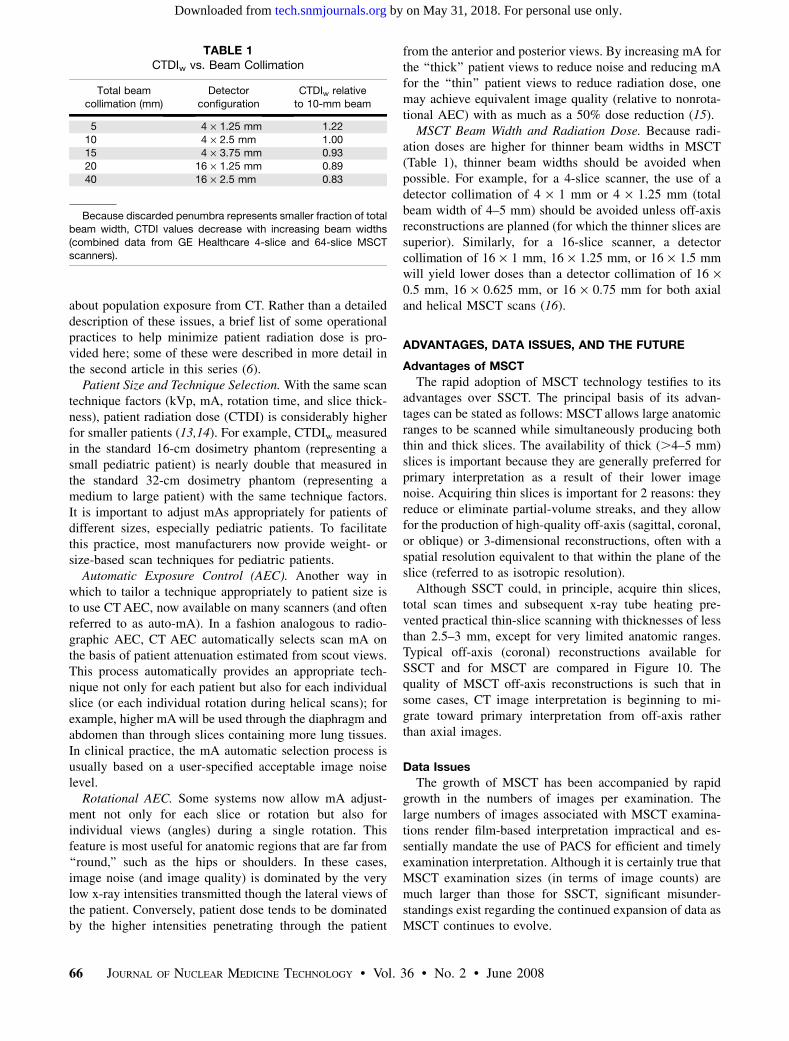
Although SSCT could, in principle, acquire thin slices,total scan times and subsequent x-ray tube heating pre-vented practical thin-slice scanning with thicknesses of lessthan 2.5–3 mm, except for very limited anatomic ranges.Typical off-axis (coronal) reconstructions available forSSCT and for MSCT are compared in Figure 10. Thequality of MSCT off-axis reconstructions is such that insome cases, CT image interpretation is beginning to mi-grate toward primary interpretation from off-axis ratherthan axial images.

Data Issues

The growth of MSCT has been accompanied by rapidgrowth in the numbers of images per examination. Thelarge numbers of images associated with MSCT examina-tions render film-based interpretation impractical and es-sentially mandate the use of PACS for efficient and timelyexamination interpretation. Although it is certainly true thatMSCT examination sizes (in terms of image counts) aremuch larger than those for SSCT, significant misunder-standings exist regarding the continued expansion of data asMSCT continues to evolve.

TABLE 1CTDIw vs. Beam Collimation

Total beam

collimation (mm)

Detector

configuration

CTDIw relative

to 10-mm beam

5 4 · 1.25 mm 1.22

10 4 · 2.5 mm 1.0015 4 · 3.75 mm 0.93

20 16 · 1.25 mm 0.89

40 16 · 2.5 mm 0.83

Because discarded penumbra represents smaller fraction of total

beam width, CTDI values decrease with increasing beam widths

(combined data from GE Healthcare 4-slice and 64-slice MSCTscanners).




With the introduction of 4-slice MSCT, the sizes of many(but not all) studies increased by 4- or 5-fold or more. Thisincrease was attributable not so much to collecting 4 slicesat once but rather to MSCT scanning of large sections ofanatomy with thin slices (2.5 mm or less), relative to SSCTscanning of the same anatomy with 5- to 10-mm slices. Forexample, covering a 40-cm scan range with contiguous5-mm slices (whether acquired axially or helically) wouldgenerate 80 images. MSCT scanning of the same rangewith a collimation of 4 · 1.25 mm to produce both 1.25-and 5-mm slices would generate 400 images: 320 imageswith a thickness of 1.25 mm and 80 images with a thicknessof 5 mm.

The reason for the large increase in image counts in theexample just given is coverage of the same anatomic rangewith both thin and thick slices rather than simultaneousacquisition of multiple images. A 16-slice scanner coveringthe same anatomy with a collimation of 16 · 1.25 mm(again reconstructed into both 1.25- and 5 mm slices)would also yield 400 images—but it would obtain them 4times faster (assuming an equivalent rotation time). On theother hand, if the same 40-cm area were scanned with acollimation of 16 · 0.625 mm to produce 0.625- and 5 mmslices, then 720 images would result (640 images of 0.625-mm slices and 80 images of 5-mm slices). A 64-slicemachine scanning the same area to produce 0.625- and5-mm slices would also generate 720 images. In general,the numbers of images produced by MSCT are associatedwith detector collimation and how the data are used ratherthan with the numbers of simultaneously acquired slices.How many slices an MSCT scanner can acquire simulta-neously affects how fast images are acquired—not howmany images are acquired.

Although scanners capable of collecting more than 64slices are now either available or in clinical trials, it isunlikely that detector element size and therefore minimumdetector collimation will continue to shrink. Because cur-

rent element sizes (typically 0.5–0.75 mm) are alreadycomparable to detector element sizes within the slice plane(see, for example, the in-plane and z-direction dimensionsof the 0.625-mm elements in Fig. 5), still-smaller z-axiselements lead to diminishing returns. Thus, except perhapsfor new and special applications, such as cardiac CT angi-ography (CTA) (see next section), the numbers of images inMSCT examinations are unlikely to increase significantly.

Cardiac MSCT

The application that currently seems to be driving state-of-the-art MSCT is CTA. Except for cardiac screeningapplications with electron-beam CT, cardiac imaging hasbeen a difficult hurdle for CT because of its demandingperformance requirements. In most cases, the optimal timefor scan data collection is during a relatively motionless-heart window of time (lasting about 175 ms for a heartbeating at 60 beats per minute) occurring at approximately65%–75% of the R-R interval. Because of this very shorttime interval, CTA examinations are electrocardiographi-cally gated helical scans with data acquired during the sameheart phase over several heartbeats. Small beam pitches(0.25 or less) are used to ensure the collection of data forslice interpolation during appropriate rotational tube posi-tions. For optimal examination quality, data associated withthe reconstruction of individual slices should be collectedduring a single beat, with the entire heart being covered inas few beats as possible (17).

Steps toward meeting these requirements have led tofaster rotation times and larger z-axis fields of view.Normally, individual cardiac axial images are reconstructedfrom ‘‘half-scan’’ data (i.e., data collected over a half rotation[180�] plus the fanbeam angle, or about 210�) rather thanfrom 360� of data. Currently, the fastest rotation times are onthe order of 1/3 s. At this speed, half-scan data can often beacquired during a single beat or, at most, 2 beats. Furtherspeed improvements are difficult to achieve because of bothmechanical stresses and x-ray output limitations. A possiblesolution now in clinical use by one manufacturer involves2 x-ray tubes and detector arrays, so that each tube–detectorpair need only complete a quarter rotation (taking about85 ms) to acquire half-scan data.

To allow coverage of the entire heart in as few beats aspossible, z-axis fields of view have increased to a currentmaximum of 40 mm. One manufacture has begun clinicaltrials of a 256-slice MSCT scanner with a 128-mm z-axisfield of view (but with a slower [0.5-s] rotation time) (18).

CONCLUSION

MSCT will continue to evolve. Most likely, future MSCTtechnology advances will be aimed at improving CTA.Except for CTA and a few other examinations that benefitfrom greater speed or large z-axis fields of view, it isunclear at this point whether additional, significant clinicaladvantages will accrue beyond those of 16-slice MSCT.

FIGURE 10. Coronal images formed from off-axis reformat-ting. (A) Thicker slices collected by SSCT lead to poor-quality,less efficacious off-axis images. (B) Thinner slices collected byMSCT lead to high-quality reformatted images, often withresolution equivalent to that within slice plane. collim 5

collimation.




Because z-axis resolution and scan quality are essentiallyidentical, the gain seems to be mostly in scan times, whichare already extraordinarily short for 16-slice scanners.Whether 16 slice, 64 slice, or beyond, MSCT will continueto grow in importance as a primary diagnostic imaging tool.

APPENDIX

z-Spacing of Parallel Opposed Rays in Helical CT

The spacing along the z-axis of measurements (samples)used to interpolate helical CT slices affects the presence ofhelical artifacts in images: the smaller the spacing, the lesssevere the artifacts. Although diagrams such as those inFigures 7 and 8 are often used to illustrate helical z-spacing,they are somewhat misleading. Parallel opposed rays usedfor interpolation (or z filtering) are separated by a half rota-tion (180�) only for detectors at the center of the fanbeamdetector array (i.e., at the center of the array within theplane of the slice). Thus, parallel opposed rays occur whenthe x-ray tube is on the exact opposite side of the patient.

For all other detectors, parallel opposed rays occur atsome other point during the rotation (either less than ormore than a half rotation), depending on the location of thedetector within the fanbeam array: the closer the detector isto the end of the array, the farther from a half rotation theparallel opposed ray occurs.

REFERENCES

1. Goldman L. Principles of CT and evolution of CT technology. In: Goldman LW,

Fowlkes JB, eds. Categorical Course in Diagnostic Radiology Physics: CT and

US Cross-Sectional Imaging. Oak Brook, IL: Radiological Society of North

America; 2000:33–52.

2. McCollough C, Zink F. Performance evaluation of a multi-slice CT system. Med Phys.

1999;26:2223–2230.

3. Flohr TG, Schaller S, Stierstorfer K, Bruder H, Ohnesorge BM, Schoepf UJ.

Multi-detector row CT systems and image-reconstruction techniques. Radiology.

2005;235:756–773.

4. Lewis M, Keat N, Edyvean S. 16 Slice CT scanner comparison report version 14.

Report 06012, Feb-06. Available at: http://www.impactscan.org/reports/Re-

port06012.htm. Accessed March 26, 2008.

5. Lewis M, Keat N, Edyvean S. 32 - 64 Slice CT scanner comparison report

version 14. Report 06013, Feb-06. Available at: http://www.impactscan.org/

reports/Report06013.htm. Accessed March 26, 2008.

6. Goldman LW. Principles of CT: radiation dose and image quality. J Nucl Med

Technol. 2007;35:213–225.

7. Hsieh J. Investigation of the slice sensitivity profile for step-and-shoot mode

multi-slice computed tomography. Med Phys. 2001;28:491–500.

8. Goldman LW. Principles of CT and CT technology. J Nucl Med Technol.

2007;35:115–128.

9. Kalender W. Principles and performance of single- and multislice spiral CT. In:

Goldman LW, Fowlkes JB, eds. Categorical Course in Diagnostic Radiology

Physics: CT and US Cross-Sectional Imaging. Oak Brook, IL: Radiological

Society of North America; 2000:127–142.

10. Hu H. Multi-slice helical CT: scan and reconstruction. Med Phys. 1999;26:5–18.

11. Wang G, Vannier M. The effect of pitch in multislice spiral/helical CT.

Med Phys. 1999;26:2648–2653.

12. La Riviere P, Pan X. Pitch dependence of longitudinal sampling and aliasing

effects in multi-slice helical computed tomography (CT). Phys Med Biol. 2002;

47:2797–2810.

13. Nickoloff E, Dutta A, Lu Z. Influence of phantom diameter, kVp and scan mode

upon computed tomography dose index. Med Phys. 2003;30:395–402.

14. Siegel M, Schmidt B, Bradly D, Suess C, Hildebolt C. Radiation dose and image

quality in pediatric CT: effect of technical factors and phantom size and shape.

Radiology. 2004;233:515–522.

15. Kalender W, Heiko W, Suess C. Dose reduction in CT by anatomically adapted

tube current modulation. II. Phantom measurements. Med Phys. 1999;26:2248–2253.

16. Mahesh M, Scatarige J, Copper J, Fishman E. Dose and pitch relationship for a

particular multislice CT scanner. AJR. 2001;177:1273–1275.

17. Hoffmann U, Ferencik M. Cury RC, Pena AJ. Coronary CT angiography. J Nucl

Med. 2006;47:797–806.

18. Shinichiro M, Endo M, Tsunoo T, et al. Physical performance evaluation of

a 256-slice CT-scanner for four-dimensional imaging. Med Phys. 2004;31:

1348–1356.




Doi: 10.2967/jnmt.107.044826Published online: May 15, 2008.

2008;36:57-68.J. Nucl. Med. Technol. Lee W. Goldman Principles of CT: Multislice CT

http://tech.snmjournals.org/content/36/2/57This article and updated information are available at:

http://tech.snmjournals.org/site/subscriptions/online.xhtml

Information about subscriptions to JNMT can be found at:

http://tech.snmjournals.org/site/misc/permission.xhtmlInformation about reproducing figures, tables, or other portions of this article can be found online at:

(Print ISSN: 0091-4916, Online ISSN: 1535-5675)1850 Samuel Morse Drive, Reston, VA 20190.SNMMI | Society of Nuclear Medicine and Molecular Imaging

is published quarterly.Journal of Nuclear Medicine Technology

© Copyright 2008 SNMMI; all rights reserved.


http://tech.snmjournals.org/content/36/2/57

http://tech.snmjournals.org/site/misc/permission.xhtml

http://tech.snmjournals.org/site/subscriptions/online.xhtml


principles of ct: multislice ct* - journal of nuclear...

Documents