Probabilistic modeling of tephra dispersion: hazard assessment of a multi-phase eruption at

Tarawera Volcano, New Zealand

C. Bonadonna1, C.B. Connor2, B.F. Houghton1,L. Connor2, M. Byrne3, A. Laing3, T.K. Hincks4

1Department of Geology and Geophysics, University of Hawaii, Honolulu, HI 96822, USA 2Department of Geology, University of South Florida, Tampa, FL 33620, USA

3Department of Geography, University of South Florida, Tampa, FL 33620, USA 4Department of Earth Sciences, University of Bristol, Bristol, BS8 1RJ, UK

2

Abstract

The Tarawera Volcanic Complex (New Zealand) comprises 11 rhyolite domes formed

during five major eruptions between 17000 BC and AD 1886, the first four of which were

predominantly rhyolitic. The only historical event (AD 1886) erupted about 2 km3 of

purely basaltic tephra fall killing about 150 people. The AD 1305 Kaharoa eruption is the

youngest rhyolitic event and erupted a total tephra-fall volume more than two times

larger than the AD 1886 eruption. We used data from the AD 1305 Kaharoa eruption to

assess the tephra-fall hazard from a future episode at Tarawera. This eruption consisted of

a complex sequence of eruptive events with eleven discrete Plinian episodes,

characterized by VEI 4. We developed an advection-diffusion model (TEPHRA) that

includes grainsize-dependent diffusion law and particle density, a stratified atmosphere,

the horizontal diffusion time of particles within the eruptive plume and settling velocities

that account for Reynold’s Number variations along the particle trajectory. Selected

eruption parameters are sampled stochastically, possible outcomes are analyzed

probabilistically and simulations are run in parallel on multiple processors. Given the fast

computational times, TEPHRA is also characterized by a robust algorithm and high

resolution and reliability of resulting outputs (i.e. hazard maps). Therefore, TEPHRA is

an example of a class of numerical models that take advantage of new computational

tools to forecast hazards as conditional probabilities far in advance of future eruptions.

Three different scenarios were investigated on a probabilistic basis for a comprehensive

tephra-fall hazard assessment: Upper Limit Scenario, Eruption-Range Scenario and

Multiple-Eruption Scenario.

3

1. Introduction Numerical models are increasingly important in geological hazards and risk

assessments [Barberi et al., 1990; Bonadonna et al., 2002a; Connor et al., 2001; Glaze

and Self, 1991; Hill et al., 1998; Iverson et al., 1998; Wadge et al., 1998]. These models

are used to quantify assessments that are otherwise based on qualitative, sometimes

disparate geological observations [Newhall and Hoblitt, 2002]. Numerical simulations (i)

augment direct observations; (ii) characterize better the variation and uncertainty in

geologic processes that often occur on long time scales, or infrequently, compared with

the time scales of human experience; (iii) allow volcanologists to explore a much wider

range of geological processes than is possible to observe directly. Therefore, evaluating

the range of possible outcomes of geologic processes, such as earthquakes, volcanic

eruptions, and landslides, is best achieved using probabilistic techniques that propagate

uncertainty through the analysis using stochastic simulations.

This is certainly true in volcanology, a field in which hazard assessments must

strive to bound the range of possible consequences of volcanic activity, drawing from the

geologic record, analogy, and understanding of the physics of volcanic processes.

Historically, volcanology has advanced through description of volcanic processes and

their impacts (e.g. Vesuvius, [Maulucci Vivolo, 1994]; Mt Pelee, [Lacroix, 1904];

Nevado del Ruiz, [Chung, 1991]). While extremely important, this approach is no longer

sufficient for mitigation of volcanic risks and numerical simulations should be used to

complement direct observations. However, such an approach is computationally

expensive, because numerical models of geologic processes are generally complex, and

because a large number of simulations is required to accurately simulate the range of

behaviors of natural phenomena, like volcanic eruptions. Nevertheless, recent advances

in parallel computing, such as the development of the Message Passing Interface (MPI)

and the advent of inexpensive computer clusters [Sterling et al., 1999], render this

approach to geological hazard assessment tractable.

As a practical example, we describe the probabilistic assessment of hazards

related to dispersion and accumulation of volcanic tephra fall, and, in particular, we

4

present the tephra-fall hazard assessment of Tarawera Volcano (New Zealand) based on

its most recent rhyolitic Plinian eruption (AD 1305 Kaharoa eruption, [Sahetapy-Engel,

2002]). Tarawera Volcano is located in the North Island of New Zealand and has been

one of New Zealand’s most destructive volcanoes in recent times. Famous for its large

eruption in 1886, Tarawera Volcano buried seven villages, killing about 150 people

[Keam, 1988]. The AD 1305 Kaharoa eruption produced a total tephra-fall volume nearly

three times larger than the AD 1886 eruption, covering a wider area northwest and

southeast of the volcano, and therefore we consider it as the appropriate scenario for our

hazard assessment of tephra fall from Tarawera Volcano. Based on the frequency of past

eruptions from this volcano complex, the annual probability of an eruption from

Tarawera with volume exceeding 0.5 km3 is approximately 10-3/yr [Stirling and Wilson,

2002], certainly a sufficiently high probability to require assessment of eruption

consequences [Woo, 2000].

This tephra-fall hazard assessment is achieved through implementation of an

advection-diffusion model (TEPHRA) derived from the integration of several modeling

approaches and theories [Armienti et al., 1988; Bonadonna et al., 1998; Bonadonna et al.,

2002a; Bonadonna and Phillips, 2003; Bursik et al., 1992a; Connor et al., 2001;

Macedonio et al., 1988; Suzuki, 1983]. TEPHRA is written for parallel computation on a

Beowulf cluster, a networked set of personal computers. As such, TEPHRA is an

example of a class of numerical models that take advantage of new computational tools to

forecast hazards as conditional probabilities far in advance of future eruptions. That is,

given that a scenario of volcanic activity takes place, what is the expected range of

tephra-fall thicknesses over a region of interest? What drives uncertainty in hazard

assessment? What eruptive conditions result in hazardous tephra-fall accumulations? Our

goal is to illustrate how numerical models, like TEPHRA, can help resolve such

questions and provide a basis for improved hazard assessment.

2. Geological setting The Tarawera Volcanic Complex is a dome complex within the Okataina

Volcanic Centre, one of the five major calderas within the Taupo Volcanic Zone, North

5

Island, New Zealand (Fig. 1). Tarawera is made of 11 rhyolite domes and a combination

of tephra-fall and flow deposits that formed during five major eruptions [Cole, 1970]: (i)

AD 1886; (ii) Kaharoa, AD 1305; (iii) Waiohau, 11000 BP; (iv) Rerewhakaaitu, 15000

BP; (v) eruption associated with the Okareka Ash, 17000 BP. The AD 1886 subplinian

eruption was basaltic. The most recent rhyolitic eruption occurred about 700 years ago

(Kaharoa eruption), and has been intensely studied in the last 5 years [Nairn, 1989; Nairn

et al., 2001; Sahetapy-Engel, 2002].

2.1 AD 1305 Kaharoa eruption

The AD 1305 Kaharoa eruption represents the most recent rhyolitic event in the

whole Taupo Volcano Zone. It consisted of a sequence of 11 Plinian eruptive episodes

with Volcano Explosivity Index (VEI) 4, column heights between about 16 and 26 km,

and volumes between about 0.2 and 1 km3 (minimum total volume is 4.6 km3, 2.2 Dense

Rock Equivalent, DRE) [Sahetapy-Engel, 2002]. Sahetapy-Engel [2002] divides the

Kaharoa tephra-fall stratigraphy in two main deposit lobes: one to the southeast and one

to the north-northwest of the volcano (Fig. 2). Detailed study of these lobes also revealed

pronounced layering of fall deposits, which were classified as Units A to L

corresponding to the 11 Plinian eruptive episodes [Sahetapy-Engel, 2002].

The Kaharoa eruption was characterized by multiple vents, but the exact location

of eruptive vents for each Unit is still uncertain. By extrapolations of the axes of dispersal

and clast size distribution Sahetapy-Engel [2002] concludes that: Units A-G were

dispersed to the southeast and were probably erupted from Crater Dome; Unit H was

dispersed to both southeast and northwest and was probably erupted from the Ruawahia

Dome; Units I-K were dispersed to the north-northwest and were also probably erupted

from the Ruawahia Dome and/or Wahanga Dome (Fig. 1).

Unit F is the one characterized by the largest volume (minimum volume of 1 km3)

and highest plume (26.4 km), whereas Units A and G have the smallest volume

(minimum volume of 0.16 km3) and lowest plumes (16.3 km). Unit K is the most

voluminous phase of the late stage of the eruption (0.79 km3) [Sahetapy-Engel, 2002].

6

The average density of analyzed pumice and lithic fragments is 1000 and 2350 kg

m-3 respectively, whereas the average bulk deposit density is 1000 kg m-3 [Sahetapy-

Engel, 2002]. High pumice density values are due to the high crystal content and low

vesicularity. An average maximum wind speed of 20-30 m s-1 and a duration of 2-6 hours

for individual eruptive episodes (with the only exception being 19 hours for episode K)

were calculated by using the method of Carey and Sparks [1986] and Sparks [1986]

[Sahetapy-Engel, 2002].

Studying the wind-field patterns throughout a whole year, Sahetapy-Engel [2002]

shows how it is likely that the whole Kaharoa eruption had a maximum duration of the

first explosive phase (episodes A-G) of 13 days. Estimates of the duration of the total

Kaharoa eruption vary between weeks to a few months, depending on the values assigned

to breaks in the eruption and the duration of dome growth and disruption [Sahetapy-

Engel, 2002].

3. TEPHRA TEPHRA consists of three main parts: (i) a physical model that describes

diffusion, transport and sedimentation of volcanic particles [Armienti et al., 1988;

Bonadonna et al., 1998; Bonadonna et al., 2002a; Bursik et al., 1992a; Connor et al.,

2001; Suzuki, 1983]; (ii) a probabilistic approach used to identify a range of input

parameters for the physical model (i.e. column height; eruption duration; mass

distribution parameter; clast exit velocity; grainsize parameters) and to forecast a range of

possible outcomes (i.e. hazard curves and probability maps); (iii) a computational

approach that uses parallel processing methods to speed up computation and make fully

probabilistic approaches practical.

3.1 Physical model

TEPHRA is written in C with MPI commands. Particle diffusion, advection and

sedimentation are computed solving a mass-conservation equation [Armienti et al., 1988;

Suzuki, 1983]. Particles of size fraction j are released from a point source i along a

7

volcanic plume. Each particle size fraction, j, and point source i is processed

independently due to the linearity of the equation. That is, the total mass oM (kg) of the

eruption is:

max

min

,0

Ho o

i ji j

M M (1)

where ,oi jM (kg) is the total mass fraction of particles with size j that fall from a point

source i at a height zi, H is the total height of the volcanic plume and min and max

indicate the maximum and minimum particle diameter respectively (with = -log2d,

where d is the particle diameter in mm). The fraction of ,oi jM (kg) that accumulates on the

ground at a certain point with coordinates (x,y) is ),(, yxm ji (kg m-2), where:

0, , ,( , ) ( , )i j i j i jm x y M f x y (2)

where ),(, yxf ji (m-2) is a function, described in detail in the following, that uses an

advection-diffusion equation to estimate the fraction of mass of a given particle size and

release height to fall around the point with coordinates (x,y). Therefore, the total mass M

accumulated per unit area (kg m-2) at a certain point on the ground (x,y) is:

max

min

,0

( , ) ( , )H

i ji

M x y m x y (3)

which is the quantity of greatest interest in forecasting volcanic hazards related to tephra

fall. Thus, the problem reduces to understanding the function, ),(, yxf ji , which controls

the horizontal dispersion of particles, and jioM , , the source term.

8

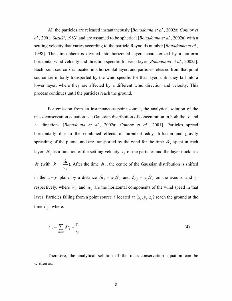
All the particles are released instantaneously [Bonadonna et al., 2002a; Connor et

al., 2001; Suzuki, 1983] and are assumed to be spherical [Bonadonna et al., 2002a] with a

settling velocity that varies according to the particle Reynolds number [Bonadonna et al.,

1998]. The atmosphere is divided into horizontal layers characterized by a uniform

horizontal wind velocity and direction specific for each layer [Bonadonna et al., 2002a].

Each point source i is located in a horizontal layer, and particles released from that point

source are initially transported by the wind specific for that layer, until they fall into a

lower layer, where they are affected by a different wind direction and velocity. This

process continues until the particles reach the ground.

For emission from an instantaneous point source, the analytical solution of the

mass-conservation equation is a Gaussian distribution of concentration in both the x and

y directions [Bonadonna et al., 2002a; Connor et al., 2001]. Particles spread

horizontally due to the combined effects of turbulent eddy diffusion and gravity

spreading of the plume, and are transported by the wind for the time jt spent in each

layer. jt is a function of the settling velocity jv of the particles and the layer thickness

z (with j

j vzt ). After the time jt , the centre of the Gaussian distribution is shifted

in the yx plane by a distance jxj twx and jyj twy on the axes x and y

respectively, where xw and yw are the horizontal components of the wind speed in that

layer. Particles falling from a point source i located at iii zyx ,, reach the ground at the

time jit , , where:

,i

i j jlayers j

zt tv

(4)

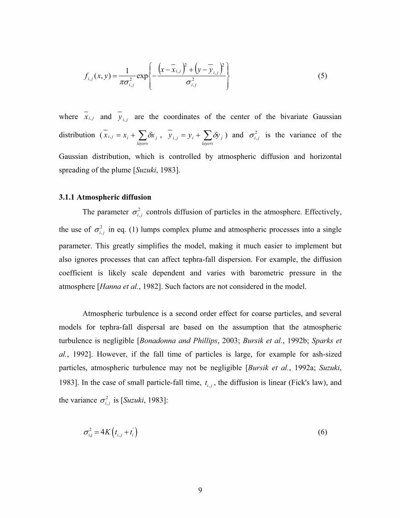
Therefore, the analytical solution of the mass-conservation equation can be

written as:

9

2,

2

,

2,

2,

, exp1),(ji

jiji

jiji

yyxxyxf (5)

where jix , and jiy , are the coordinates of the center of the bivariate Gaussian

distribution (layers

jiji xxx , ,layers

jiji yyy , ) and 2,i j is the variance of the

Gaussian distribution, which is controlled by atmospheric diffusion and horizontal

spreading of the plume [Suzuki, 1983].

3.1.1 Atmospheric diffusion

The parameter 2,i j controls diffusion of particles in the atmosphere. Effectively,

the use of 2,i j in eq. (1) lumps complex plume and atmospheric processes into a single

parameter. This greatly simplifies the model, making it much easier to implement but

also ignores processes that can affect tephra-fall dispersion. For example, the diffusion

coefficient is likely scale dependent and varies with barometric pressure in the

atmosphere [Hanna et al., 1982]. Such factors are not considered in the model.

Atmospheric turbulence is a second order effect for coarse particles, and several

models for tephra-fall dispersal are based on the assumption that the atmospheric

turbulence is negligible [Bonadonna and Phillips, 2003; Bursik et al., 1992b; Sparks et

al., 1992]. However, if the fall time of particles is large, for example for ash-sized

particles, atmospheric turbulence may not be negligible [Bursik et al., 1992a; Suzuki,

1983]. In the case of small particle-fall time, ,i jt , the diffusion is linear (Fick's law), and

the variance 2,i j is [Suzuki, 1983]:

2 'i,j ,4 i j iK t t (6)

10

where K (m2 s-1) is a constant diffusion coefficient, ,i jt (s) is the total particle fall time

(eq. (4)), and 'it (s) is the horizontal diffusion time in the volcanic plume. The horizontal

diffusion coefficient, K , is considered isotropic (K=Kx=Ky) [Armienti et al., 1988;

Bonadonna et al., 2002a; Connor et al., 2001; Suzuki, 1983]. The vertical diffusion

coefficient is small above 500 m of altitude [Pasquill, 1974], and therefore is assumed to

be negligible. The horizontal diffusion time, 'it , accounts for the change in width of the

plume as a function of height. Change in width of the ascending turbulent plume is

complex [Ernst et al., 1996; Woods, 1995] and also includes the gravitational spreading

should the plume reach neutral buoyancy [Sparks, 1986]. Such a change in plume width

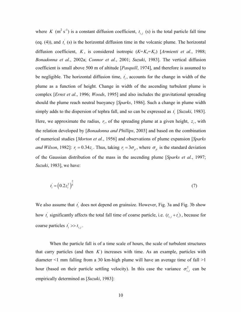
simply adds to the dispersion of tephra fall, and so can be expressed as 'it [Suzuki, 1983].

Here, we approximate the radius, ir , of the spreading plume at a given height, iz , with

the relation developed by [Bonadonna and Phillips, 2003] and based on the combination

of numerical studies [Morton et al., 1956] and observations of plume expansion [Sparks

and Wilson, 1982]: 0.34i ir z . Thus, taking 3i pr , where p is the standard deviation

of the Gaussian distribution of the mass in the ascending plume [Sparks et al., 1997;

Suzuki, 1983], we have:

2' 2 50.2i it z (7)

We also assume that 'it does not depend on grainsize. However, Fig. 3a and Fig. 3b show

how 'it significantly affects the total fall time of coarse particle, i.e. '

,( )i j it t , because for

coarse particles jii tt ,' .

When the particle fall is of a time scale of hours, the scale of turbulent structures

that carry particles (and then K ) increases with time. As an example, particles with

diameter <1 mm falling from a 30 km-high plume will have an average time of fall >1

hour (based on their particle settling velocity). In this case the variance 2,i j can be

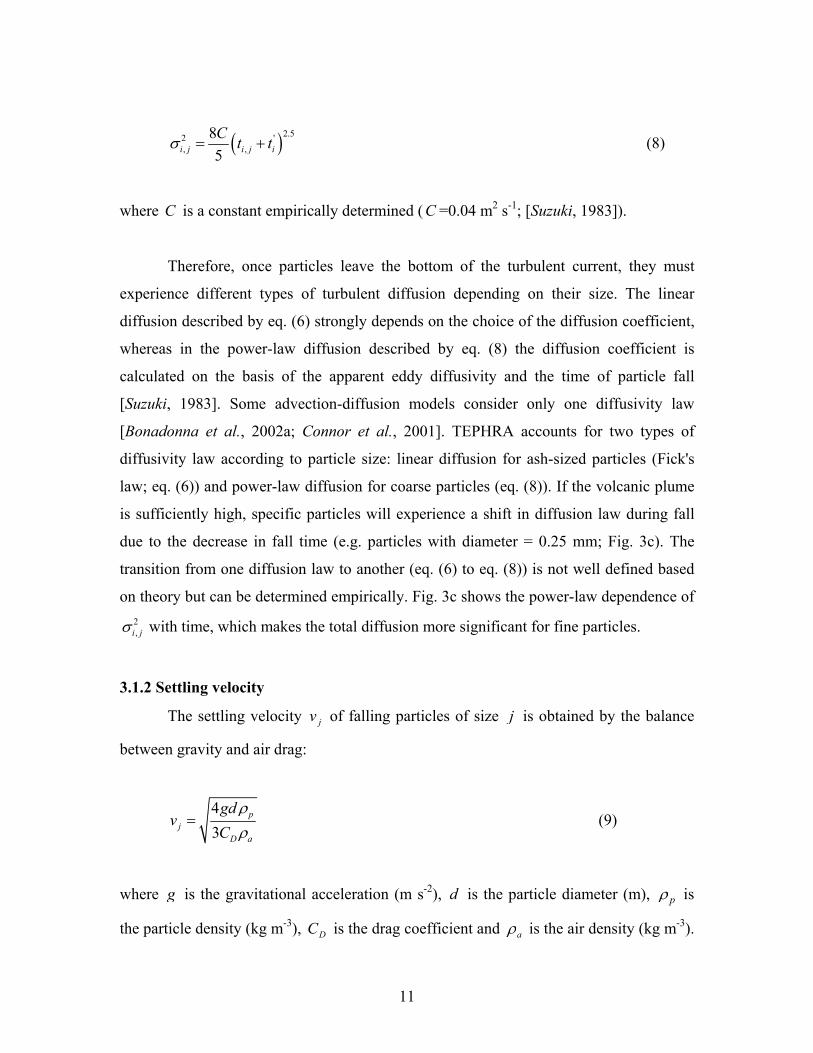
empirically determined as [Suzuki, 1983]:

11

2.52 ', ,

85i j i j iC t t (8)

where C is a constant empirically determined ( C =0.04 m2 s-1; [Suzuki, 1983]).

Therefore, once particles leave the bottom of the turbulent current, they must

experience different types of turbulent diffusion depending on their size. The linear

diffusion described by eq. (6) strongly depends on the choice of the diffusion coefficient,

whereas in the power-law diffusion described by eq. (8) the diffusion coefficient is

calculated on the basis of the apparent eddy diffusivity and the time of particle fall

[Suzuki, 1983]. Some advection-diffusion models consider only one diffusivity law

[Bonadonna et al., 2002a; Connor et al., 2001]. TEPHRA accounts for two types of

diffusivity law according to particle size: linear diffusion for ash-sized particles (Fick's

law; eq. (6)) and power-law diffusion for coarse particles (eq. (8)). If the volcanic plume

is sufficiently high, specific particles will experience a shift in diffusion law during fall

due to the decrease in fall time (e.g. particles with diameter = 0.25 mm; Fig. 3c). The

transition from one diffusion law to another (eq. (6) to eq. (8)) is not well defined based

on theory but can be determined empirically. Fig. 3c shows the power-law dependence of 2,i j with time, which makes the total diffusion more significant for fine particles.

3.1.2 Settling velocity

The settling velocity jv of falling particles of size j is obtained by the balance

between gravity and air drag:

43

pj

D a

gdv

C (9)

where g is the gravitational acceleration (m s-2), d is the particle diameter (m), p is

the particle density (kg m-3), DC is the drag coefficient and a is the air density (kg m-3).

12

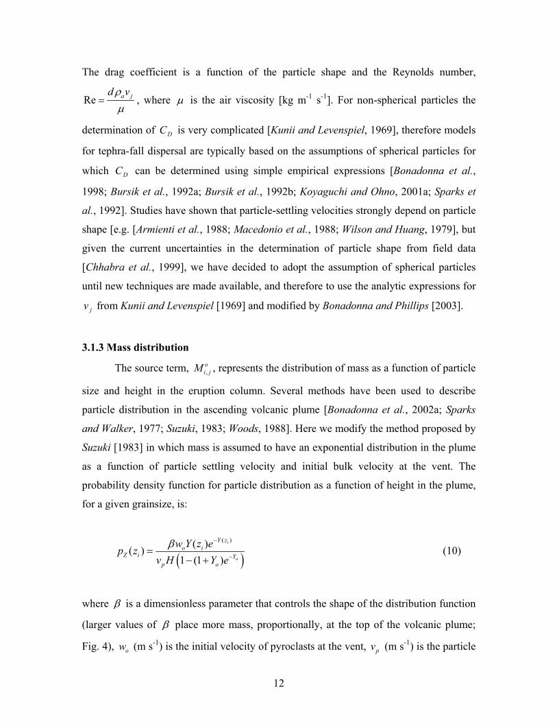
The drag coefficient is a function of the particle shape and the Reynolds number,

Re a jd v, where is the air viscosity [kg m-1 s-1]. For non-spherical particles the

determination of DC is very complicated [Kunii and Levenspiel, 1969], therefore models

for tephra-fall dispersal are typically based on the assumptions of spherical particles for

which DC can be determined using simple empirical expressions [Bonadonna et al.,

1998; Bursik et al., 1992a; Bursik et al., 1992b; Koyaguchi and Ohno, 2001a; Sparks et

al., 1992]. Studies have shown that particle-settling velocities strongly depend on particle

shape [e.g. [Armienti et al., 1988; Macedonio et al., 1988; Wilson and Huang, 1979], but

given the current uncertainties in the determination of particle shape from field data

[Chhabra et al., 1999], we have decided to adopt the assumption of spherical particles

until new techniques are made available, and therefore to use the analytic expressions for

jv from Kunii and Levenspiel [1969] and modified by Bonadonna and Phillips [2003].

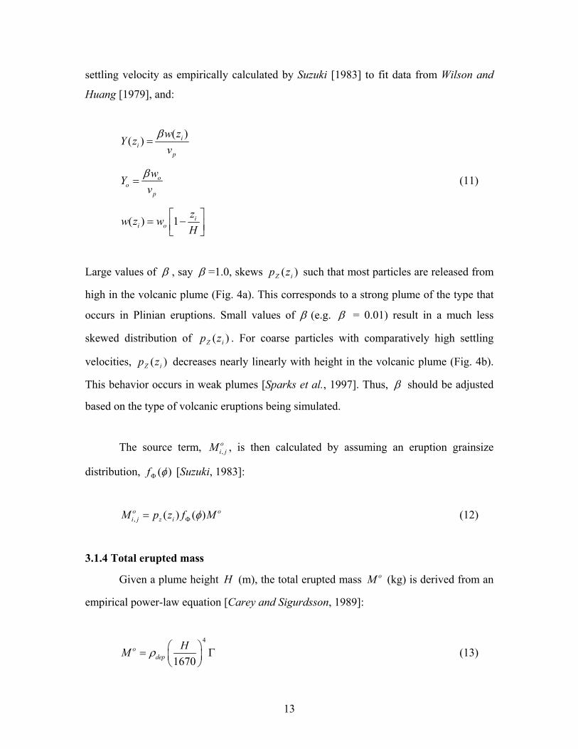
3.1.3 Mass distribution

The source term, ,oi jM , represents the distribution of mass as a function of particle

size and height in the eruption column. Several methods have been used to describe

particle distribution in the ascending volcanic plume [Bonadonna et al., 2002a; Sparks

and Walker, 1977; Suzuki, 1983; Woods, 1988]. Here we modify the method proposed by

Suzuki [1983] in which mass is assumed to have an exponential distribution in the plume

as a function of particle settling velocity and initial bulk velocity at the vent. The

probability density function for particle distribution as a function of height in the plume,

for a given grainsize, is:

( )( )( )1 (1 )

i

o

Y zo i

Z i Yp o

w Y z ep zv H Y e

(10)

where is a dimensionless parameter that controls the shape of the distribution function

(larger values of place more mass, proportionally, at the top of the volcanic plume;

Fig. 4), ow (m s-1) is the initial velocity of pyroclasts at the vent, pv (m s-1) is the particle

13

settling velocity as empirically calculated by Suzuki [1983] to fit data from Wilson and

Huang [1979], and:

( )( ) ii

p

w zY zv

oo

p

wYv

(11)

( ) 1 ii o

zw z wH

Large values of , say =1.0, skews )( iZ zp such that most particles are released from

high in the volcanic plume (Fig. 4a). This corresponds to a strong plume of the type that

occurs in Plinian eruptions. Small values of (e.g. = 0.01) result in a much less

skewed distribution of )( iZ zp . For coarse particles with comparatively high settling

velocities, )( iZ zp decreases nearly linearly with height in the volcanic plume (Fig. 4b).

This behavior occurs in weak plumes [Sparks et al., 1997]. Thus, should be adjusted

based on the type of volcanic eruptions being simulated.

The source term, ,oi jM , is then calculated by assuming an eruption grainsize

distribution, )(f [Suzuki, 1983]:

, ( ) ( )o oi j z iM p z f M (12)

3.1.4 Total erupted mass

Given a plume height H (m), the total erupted mass oM (kg) is derived from an

empirical power-law equation [Carey and Sigurdsson, 1989]:

4

1670o

depHM (13)

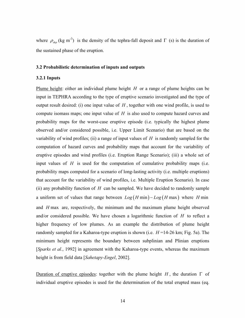
14

where dep (kg m-3) is the density of the tephra-fall deposit and (s) is the duration of

the sustained phase of the eruption.

3.2 Probabilistic determination of inputs and outputs

3.2.1 Inputs

Plume height: either an individual plume height H or a range of plume heights can be

input in TEPHRA according to the type of eruptive scenario investigated and the type of

output result desired: (i) one input value of H , together with one wind profile, is used to

compute isomass maps; one input value of H is also used to compute hazard curves and

probability maps for the worst-case eruptive episode (i.e. typically the highest plume

observed and/or considered possible, i.e. Upper Limit Scenario) that are based on the

variability of wind profiles; (ii) a range of input values of H is randomly sampled for the

computation of hazard curves and probability maps that account for the variability of

eruptive episodes and wind profiles (i.e. Eruption Range Scenario); (iii) a whole set of

input values of H is used for the computation of cumulative probability maps (i.e.

probability maps computed for a scenario of long-lasting activity (i.e. multiple eruptions)

that account for the variability of wind profiles, i.e. Multiple Eruption Scenario). In case

(ii) any probability function of H can be sampled. We have decided to randomly sample

a uniform set of values that range between min maxLog H Log H where minH

and maxH are, respectively, the minimum and the maximum plume height observed

and/or considered possible. We have chosen a logarithmic function of H to reflect a

higher frequency of low plumes. As an example the distribution of plume height

randomly sampled for a Kaharoa-type eruption is shown (i.e. H =14-26 km; Fig. 5a). The

minimum height represents the boundary between subplinian and Plinian eruptions

[Sparks et al., 1992] in agreement with the Kaharoa-type events, whereas the maximum

height is from field data [Sahetapy-Engel, 2002].

Duration of eruptive episodes: together with the plume height H , the duration of

individual eruptive episodes is used for the determination of the total erupted mass (eq.

15

(13)). TEPHRA randomly samples the duration amongst a given range of values

observed and/or considered possible. As an example the distribution of the eruptive-

episode duration randomly sampled for a Kaharoa-type eruption is shown (i.e. 2-6 hrs;

Fig. 5b).

Total erupted mass: the distribution of plume-height values described above associated

with the randomly sampled distribution of eruptive-episode duration results in a log-

normal distribution of the total erupted mass derived using eq. (13) (Fig. 5c).

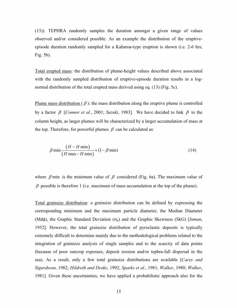
Plume mass distribution ( ): the mass distribution along the eruptive plume is controlled

by a factor [Connor et al., 2001; Suzuki, 1983]. We have decided to link to the

column height, as larger plumes will be characterized by a larger accumulation of mass at

the top. Therefore, for powerful plumes can be calculated as:

minmin (1 min)

max minH H

H H(14)

where min is the minimum value of considered (Fig. 6a). The maximum value of

possible is therefore 1 (i.e. maximum of mass accumulation at the top of the plume).

Total grainsize distribution: a grainsize distribution can be defined by expressing the

corresponding minimum and the maximum particle diameter, the Median Diameter

(Md ), the Graphic Standard Deviation ( ) and the Graphic Skewness (SkG) [Inman,

1952]. However, the total grainsize distribution of pyroclastic deposits is typically

extremely difficult to determine mainly due to the methodological problems related to the

integration of grainsize analysis of single samples and to the scarcity of data points

(because of poor outcrop exposure, deposit erosion and/or tephra-fall dispersal in the

sea). As a result, only a few total grainsize distributions are available [Carey and

Sigurdsson, 1982; Hildreth and Drake, 1992; Sparks et al., 1981; Walker, 1980; Walker,

1981]. Given these uncertainties, we have applied a probabilistic approach also for the

16

determination of the total grainsize distribution stochastically sampling Md between

values observed and/or considered possible. As an example the distribution of Md

randomly sampled for a Kaharoa-type eruption is shown (i.e. Md = -0.8 and 4 ; Fig.

6b). This is based on data from comparable Plinian eruptions: Taupo, Waimihia and

Hatepe Plinian [Walker, 1980; Walker, 1981] (Fig. 6c).

Particle exit velocity ( ow ): the particle velocity at vent is necessary to determine the

probability density function for a given grainsize in the eruptive plume (eq. (10)).

However, not many information for this parameter are known, therefore is randomly

sampled between 100-150 m s-1 for powerful eruptions based on theoretical values

[Sparks et al., 1997].

Eruptive vent: the Kaharoa eruption was characterized by at least two active eruptive

vents possibly three (Crater Dome, Ruawahia Dome and Wahanga Dome; Fig. 1). The

presence of multiple active vents is known for several eruptions (e.g. Tolbachik volcano,

[Fedotov et al., 1991]; Tarawera AD 1886 [Keam, 1988; Walker et al., 1984]; Rabaul

[Blong, 1994]) and can significantly affect the patterns of tephra-fall dispersal. Some

single-vent eruptions can also occur in volcanic areas characterized by several possible

future vents (e.g. Campi Flegrei [Di Vito et al., 1999]; Mt. Etna [Coltelli et al., 1998];

Michoacàn-Guanajuto, [Williams, 1950]). A complete hazard assessment needs to

account for all possible eruptive vents. TEPHRA can randomly sample an eruptive vent

from a set of vent coordinates considered possible.

3.2.2 Outputs

TEPHRA produces three main outputs: (i) isomass maps, (ii) hazard curves, and

(iii) probability maps. Isomass maps describe the accumulation of mass per unit area

around the volcano and are computed given one wind profile and one eruptive episode.

They are mainly used to calibrate the model and to assess the agreement with field data.

However, tephra-fall hazard assessments are based on the compilation of probabilistic

outputs, i.e. hazard curves and probability maps. Crucial to a tephra-fall hazard

17

assessment, and, in particular, to the interpretation of the probabilistic outputs, are the

hazardous deposit thresholds, i.e. values of tephra-fall mass per unit area that cause

specific types of damage (e.g. collapse of building roofs, different degrees of damage to

vegetation and crops) [Blong, 1984]. Every geographic area is characterized by specific

deposit thresholds due to different climate conditions and building structures [Blong,

1984; Bonadonna et al., 2002a].

Hazard curves

Hazard curves considered here indicate the probability of exceeding certain values of

accumulation of mass per unit area at a particular location [Hill et al., 1998; Stirling and

Wilson, 2002]. Hazard curves can be computed considering a set of eruptive episodes and

a set of wind profiles.

Probability maps

Probability maps show the probability of reaching a given mass accumulation per unit

area (i.e. hazardous deposit threshold) in a particular location given different sets of

conditions. Different types of probability maps can be compiled depending on the

specific assessment required (e.g. assessment for a specific locality; assessment for a

specific area; assessment for different eruptive scenarios). For our assessment we have

compiled:

(i) Probability maps given one eruptive episode and a set of wind profiles (Upper Limit

Scenario, ULS): given one possible eruptive episode, these maps show the probability

distribution of reaching a particular mass loading around the volcano based on the

statistical distribution of wind profiles and therefore contour:

( , ) | eruptionP M x y threshold , where all eruption parameters are specified

deterministically. This is useful to determine an upper limit value on tephra-fall

accumulation if the parameters are specified for the largest reasonable eruption for that

particular volcano.

(ii) Probability maps given a set of eruptive episodes and a set of wind profiles (Eruption

Range Scenario, ERS): given a set of possible eruptive episodes, these maps show the

probability distribution of a particular mass loading around the volcano based on the

18

statistical distribution of possible eruptive episodes and wind profiles both sampled

randomly. These maps contour: ( , ) | eruptionP M x y threshold , where all eruption

parameters and wind profiles are both sampled stochastically. The resulting map provides

a fully probabilistic hazard assessment for a given volcano.

(iii) Cumulative probability maps for a given scenario of activity and a set of wind

profiles (Multiple Eruption Scenario, MES): given a scenario of long-lasting activity (i.e.

set of eruptive episodes all happening), these maps show the probability distribution of

reaching a particular mass loading around the volcano based on the statistical distribution

of wind profiles contouring: ( , ) | scenarioP M x y threshold . These maps are important

to assess tephra-fall accumulation from multiple-phase eruptions, such as the AD 1305

Kaharoa eruption, and long-lasting eruptions, such as the 1995-1999 eruption of

Montserrat [Kokelaar, 2002; Sparks and Young, 2002]. These computed probability maps

assume continuous tephra-fall accumulation with no erosion between eruptive episodes

and are calculated using Monte Carlo simulations based on a random sampling of wind

profiles [Bonadonna et al., 2002a].

3.3 Cluster and parallelization

Numerical models used for hazard assessments of natural phenomena are

typically conceptually straightforward [Barberi et al., 1990; Bonadonna et al., 2002a;

Connor et al., 2001; Hill et al., 1998], but the application of the algorithm is made

onerous by the need to execute the same calculations for several grid points (hazard-map

resolution) and to run numerous simulations in order to capture uncertainties in the

hazard estimates (hazard-map reliability). As an example, probability maps computed on

a 450 Pentium III for a 3-year scenario of activity at the Soufrière Hills Volcano

(Montserrat, WI) would require roughly 4 days [Bonadonna et al., 2002a]. These long

computing times are not ideal when dealing with hazard assessments required during

volcanic crisis. As a result, depending on the machine available, map resolution and

reliability are often decreased to obtain shorter computational times. Finally, also the

algorithm and the initial assumptions are often simplified to speed up the calculations

(e.g. assumption of constant atmospheric density and, therefore, constant particle settling

velocity [Barberi et al., 1990; Bonadonna et al., 2002a]; assumption of uniform wind

19

field [Connor et al., 2001; Hill et al., 1998]; assumption of a single particle diffusion law

[Barberi et al., 1990; Bonadonna et al., 2002a; Connor et al., 2001; Hill et al., 1998]).

3.3.1 Beowulf cluster

TEPHRA was actually born to fulfill the need of: (i) implementation of existing

codes [Bonadonna et al., 2002a; Connor et al., 2001], (ii) probabilistic determination of

input and output parameters, (iii) improvement of the computational time. Therefore, it

was designed for parallel computation on a Beowulf cluster. A Beowulf cluster usually

consists of off-the-shelf personal computers connected by Ethernet, running Linux

operating system, and the Message Passing Interface (MPI) for parallel work. The idea of

using affordable and scalable hardware components for parallel computing is extremely

well-suited for handling the repetition required for stochastic simulations of geologic

hazards.

Our cluster consists of eight desktop computers each containing a 1.5 GHz

Pentium IV processor. All machines are equipped with an Ethernet card and linked by

Fast Ethernet and 16 port hub. In addition to these eight computers, a server node

contains two Ethernet cards that allow communication with both the private Beowulf

network and the outside network. The server node functions as both a member of the

cluster and as a cluster interface. To avoid repetitious transferring of files and programs

to each of the nodes, the cluster’s server uses the Network File System (NFS) to share

files between the server and nodes. Ease of use of this architecture is facilitated using the

Linux operation system (SuSE version 8.0) on the entire cluster.

3.3.2 Parallel code

The Message Passing Interface (MPI) libraries are freely available tools for

creating and running C, C++ or Fortran codes in parallel on a cluster of machines, such as

the Beowulf cluster described above. These libraries facilitate the message passing

between computer nodes and provide the ability to start and stop processes on every

node.

20

TEPHRA uses this master-slave relationship model. The sole job of the master

process is to orchestrate the computing that will be done by slave processes. When started

on the server node, the master process reads in the eruption parameters and the grid

dimensions from input files. The master process then starts the slave processes on all of

the nodes and decomposes the problem, distributing even portions to the slave processes

for computation. Each slave process solves for tephra-fall accumulation for some fraction

of the map grid and eruption parameters. When the slave processes are finished, they

send their results to the waiting master process and quit. The master process then finishes

by outputting the returned results on the cluster’s server node.

In our parallel implementation, the decomposition of the computational domain is

achieved by dividing the grid domain where tephra-fall deposition is to be calculated and

the master process distributes a portion of the grid to each slave. Each slave computes the

accumulation on its assigned portion and returns the results to the master process. On a

homogeneous cluster, one in which each slave process is executing on identical hardware,

the computational domain is divided and distributed equally among the identical nodes.

Each slave process, one executing on each node, begins and finishes their computations

at approximately the same time. This technique, called static decomposition [Geist et al.,

1997], works well for solving tephra-fall hazard problems.

We have found that the computational efficiency of solving the probabilistic

hazard assessment is well worth the effort of parallelizing the code. Speed-up (change in

total computational time on the cluster of processors divided by computational time on a

single processor) is linear for this type of stochastic simulation. This means that a large

number of stochastic simulations can be performed efficiently using widely available

computer components. Our experience is that this results in a far more thorough hazard

assessment than is otherwise practical.

4. Results

4.1 Calibration

21

A series of sensitivity tests were carried out to determine the best values of

diffusion coefficient, , fall-time threshold and mass-distribution parameter, . The

diffusion coefficient is crucial for the atmospheric diffusion of coarse particles, the fall-

time threshold determines the cut-off between linear and power-law atmospheric

diffusion (eq. (6) and (8)) and determines the mass distribution within the eruptive

plume (eq. (10) to eq. (12)). The best fit is determined by calculating the minimum value

of the misfit function (mf) keeping two parameters fixed at a time and varying the other

one. The misfit function for each ground point with coordinates (x,y) is expressed as:

2

1

obs compN

M Mmf

N, (15)

where N is the number of data and obsM (kg m-2) and compM (kg m-2) are the observed

and computed mass accumulation per unit area respectively [Bonadonna et al., 2002a].

The misfit function is an estimate of the global agreement between observed and

computed data, and so comparison between observations and model results was also

studied at individual locations. Unfortunately, given the age of the AD 1305 Kaharoa

eruption, a complete dataset is not available to thoroughly calibrate the model before

hazard curves and maps are computed (i.e. good mass/area data, wind data, total erupted

mass, total grainsize distribution). Therefore, sensitivity tests were carried out on a well-

studied eruption from a different volcano in New Zealand: the 17 June 1996 andesitic

subplinian eruption of Ruapehu. Such eruption produced at least 5x109 kg of tephra fall

and the corresponding tephra-fall deposit was sampled and studied in detail [Bonadonna,

2001; BF Houghton, manuscript in preparation, 2003]. The plume was bent over by a

strong SE wind and reached a maximum height of 8.5 km above sea level [Prata and

Grant, 2001].

Ruapehu

(Runs 1 and 2 in Table 1)

22

Sensitivity tests carried out on the whole Ruapehu dataset (114 samples) show a best fit

for a diffusion coefficient of 200 m2 s-1, a fall-time threshold of 72 s (i.e. 0.02 hours) and

a value of 0.2 (Fig. 7; Runs 1 in Table 1). However, the 17 June 1996 eruption of

Ruapehu produced a weak plume, which is characterized by a very different

sedimentation dynamics in proximal area compared to strong plumes. Besides, several

Ruapehu samples were collected close to the eruptive vent, and advection-diffusion

models do not reproduce the proximal deposit very accurately [e.g. Barberi et al., 1990;

Bonadonna et al., 2002a]. Therefore, sensitivity tests were also carried out to determine a

best fit of values for distal sedimentation (i.e. dataset of 88 samples collected at a

distance from vent > 5 km; Runs 2 in Table 1). Fig. 7 shows that the best fit for the distal

dataset is obtained for a diffusion coefficient of 600 m2 s-1, a fall-time threshold of 1080 s

(i.e. 0.3 hours) and a value of 0.3. Values of of 0.2 and 0.3 are in agreement with our

predictions that weak and strong plumes are characterized by small and large values of

respectively. Figs 8a and 8b show the comparison between observed and computed

accumulation mass (kg m-2) for the “best-fit” values of diffusion coefficient and fall-time

threshold for the total dataset (computed with a diffusion coefficient of 200 m2 s-1, a fall-

time threshold of 72 s and a value of 0.2) and for the distal dataset (computed with a

diffusion coefficient of 600 m2 s-1, a fall-time threshold of 1080 s and a value of 0.3).

Residual proximal data computed with the “best-fit” values obtained for the distal dataset

(i.e. diffusion coefficient of 600 m2 s-1, fall-time threshold of 1080 s and a value of 0.3)

were also plotted. Data points showing the largest misfit are those points characterized by

mass/area> 50 kg m-2 (i.e. mostly proximal points).

Kaharoa F

(Runs 3 in Table 1)

“Best-fit” values determined for the distal sedimentation of the 17 June 1996 eruption of

Ruapehu were also used to compute isomass maps for Tarawera Volcano. Fig. 8c shows

the comparison between observed data for the Unit F of the Kaharoa eruption and

computed data using the “best-fit” values obtained for the distal dataset of the Ruapehu

eruption (i.e. diffusion coefficient of 600 m2 s-1 and fall-time threshold of 1080 s; Runs 3

23

in Table 1). The best-fit values of determined for the two Ruapehu data sets

investigated (i.e. 0.2 and 0.3; Table 1 and Fig. 7) reflect the sedimentation from weak

plumes. Given that the Kaharoa F event produced a very powerful plume (H = 26.4 km),

we have used = 1 in this simulation. Wind profile was chosen with a direction in

agreement with the main axis of dispersal of the Unit F (135°N); maximum wind speed

(27 m s-1) and column height (26.4 km) were calculated using the method by Carey and

Sparks [1986] [Sahetapy-Engel, 2002]; total erupted mass (1.1x1012 kg) was calculated

using the method by Pyle [1989] [Sahetapy-Engel, 2002]; particle density was varied

between 1000-2350 kg m-3 [Sahetapy-Engel, 2002]; total grainsize distribution was

averaged between the Taupo, Waimihia and Hatepe Plinian [Walker, 1980; Walker, 1981]

(Fig. 6c).

4.2 Hazard assessment

As mentioned above we have based our tephra-fall hazard assessment of

Tarawera Volcano on the AD 1305 Kaharoa eruption, and have analyzed three different

eruptive scenarios to compile hazard curves and probability maps: Upper Limit Scenario,

Eruption Range Scenario and Multiple Eruption Scenario. ERS hazard curves and

probability maps were computed stochastically sampling 1000 different eruptions (i.e.

Md , column height, eruptive vent, , eruption duration, clast exit velocity), whereas

MES probability maps were computed using 100 sets of 10 different eruptions

stochastically sampled. ULS hazard curves and probability maps were computed running

1000 eruptions with the highest plume, the longest duration and = 1 (i.e. largest erupted

mass released from the top of the plume) and with only Md , clast exit velocity and

eruptive vent stochastically sampled. The following Kaharoa-type eruptive parameters

were used:

Plume height: for the computation of ERS hazard curves and ERS and MES probability

maps we have sampled plume heights between min maxLog H Log H where

minH =14 km and maxH =26 km (Fig. 5a). We have also computed ULS hazard curves

24

and probability maps for the highest plume determined for the Kaharoa eruption (i.e. 26

km).

Duration of eruptive episodes: the duration of eruptive episodes is randomly sampled

between 2-6 hours [Sahetapy-Engel, 2002] (Fig. 5b). We have neglected Unit K which

has a duration of 19 hours.

Plume mass distribution ( ): given that Kaharoa-type plumes are Plinian, we have

determined using eq. (14) with min =0.5, so that is made vary between 0.5-1

(Fig. 6a).

Diffusion coefficient (Ficks law) and diffusion law cut-off: best fit values for the distal

deposit produced by the 17 June 1996 eruption of Ruapehu are used for all simulations

(i.e. diffusion coefficient = 600 m2 s-1, diffusion-law cut-off = 1080 s).

Grainsize: as mentioned earlier, we have applied a probabilistic approach also for the

determination of the total grainsize of a future Kahaora-type eruption. Therefore, we have

stochastically sampled Md between -0.8 and 4 , keeping the minimum and maximum

diameter fixed at -7 and 10 , and fixed at 2.5 (Fig. 6b and 6c).

Pumice density: density of pumice fragments ( p ) is varied between 1000 and 2350 kg

m-3 according to the density parameterization used by [Bonadonna and Phillips, 2003]

and based on the average measured pumice and lithic density (1000 and 2350 kg m-3

respectively) [Sahetapy-Engel, 2002] (Fig. 10).

Bulk density of the tephra-fall deposit: average measured deposit density ( dep ) is 1000

kg m-3 [Sahetapy-Engel, 2002].

Time break amongst eruptive episodes: given the uncertainties on the total duration of the

Kaharoa eruption and the time break between individual eruptive episodes, we have

25

decided to sample wind profiles stochastically to compute MES probability maps so that

the final convergence value of probability at each grid point is independent from the time

break.

Eruptive vent: the active eruptive vent is randomly sampled amongst the three Kaharoa

eruptive vents (Crater Dome, Ruawahia Dome and Wahanga Dome; Fig. 1).

Wind data: the wind field used by TEPHRA is stratified every 1 km. For the Tarawera

assessment we have used the gridded zonal and meridional wind fields from the National

Centers for Environmental Prediction (NCEP) Reanalysis project [Kalnay et al., 1996].

Data at 17 pressure levels (1000, 925, 850, 700, 600, 500, 400, 300, 250, 200, 150, 100,

70, 50, 30, 20, and 10 hPa) were interpolated linearly to 30 geopotential height levels at 1

km intervals. Values at each height level represent the average wind velocity of the four

grid points surrounding the volcano. We have considered 3 years of wind profiles

sampled 4 times a day (00:00; 06:00; 12:00; 18:00 UTC) from 1 January 1996 through 31

December 1998. The North Island of New Zealand is in the mid-latitudes (approx.: 35°-

41° S, New Zealand Geodetic Datum 2000), therefore, winds usually blow from the west

(Fig. 11) and the tropopause heights are approximately 10 km during the winter and 15

km during the summer. Our data (1996 through 1998) also show a significant change in

mean wind direction at relatively high altitudes (>25 km above sea level), where winds

start blowing mainly from the south (Fig. 11a). The direction that the wind blows towards

to varies between about -110° and 180° from North (Fig. 11a), whereas the wind velocity

varies between about 2 and 40 m s-1 (Fig. 11b). A detailed analysis of the 1996-1998

wind data shows that 86% of wind profiles have at least 15 levels of wind blowing

between 0° and 180° from the North, whereas only 3% have at least 15 levels of wind

blowing between 180° and 360° from North (Fig. 12a). Wind is more likely to blow

between 180° and 360° during the austral spring-summer (i.e. September through March;

Fig. 12b).

Hazardous deposit thresholds: in our tephra-fall hazard assessment for Tarawera Volcano

we have considered hazardous deposit thresholds derived from observations made on

26

hazardous effects in New Zealand (D. Johnston, pers. comm.) and for a 1000 kg m-3

deposit density [Sahetapy-Engel, 2002]: 30 kg m-2 (damage to agriculture), 300 kg m-2

(minimum loading for roof collapse), 600 kg m-2 (roof collapse for all buildings). [Blong,

1984] also suggests loadings of 1800 kg m-2 and 2400 kg m-2 as the zone of near total

vegetation kill and the zone of total vegetation kill respectively.

4.2.1 Hazard curves

(Runs 4 and 5 in Table 1)

Hazard curves were computed for six key cities and towns around Tarawera

Volcano: Maketu, Kawerau, Tauranga, Taupo, Rotorua, and Wellington (Fig. 1). The

ULS hazard curves show >5% probability of reaching a tephra-fall accumulation of 10 kg

m-2 (i.e. ~ 1 cm) in all cities and towns considered except Wellington, which is

characterized by very low tephra-fall accumulation for all eruptive conditions considered

in this assessment (Fig. 13). The ERS hazard curves do not diverge significantly from the

ULS hazard curves and show >5% probability of reaching a tephra-fall accumulation of

10 kg m-2 (i.e. ~1 cm) in all localities considered except Tauranga, Taupo and

Wellington. All cities and town considered show <<0.1% probability of reaching the

minimum threshold for roof collapse (i.e. 300 kg m-2) (Fig. 13).

4.2.2 Probability Maps

(Runs 6 to 8 in Table 1)

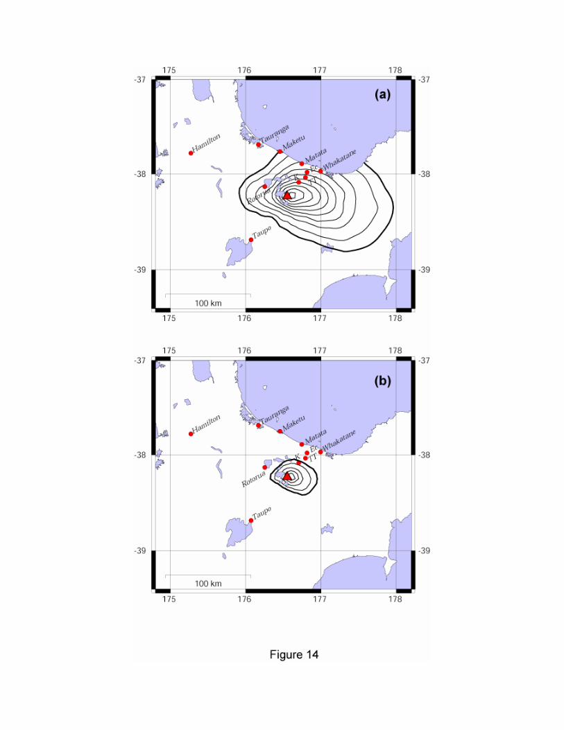
In the case where Tarawera Volcano produces a 26 km high plume (ULS maps;

Runs 6 in Table 1), Rotorua and the main populated towns northeast of Tarawera

Volcano would be likely to receive enough tephra fall to cause significant damage to

agriculture (5-65%; Fig. 14a). However, only Kawerau (small town) has a small chance

(5-10%) to experience some roof collapse in the case that Tarawera Volcano generates a

26 km high plume (Fig. 14b).

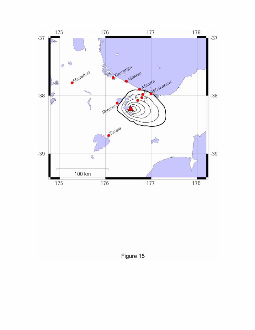
In the case where Tarawera Volcano produces a plume ranging between 14 and

26 km (ERS maps; Runs 7 in Table 1), only some populated towns northeast of Tarawera

27

would be likely to receive enough tephra fall to cause significant damage to agriculture

(5-25%; Fig. 15). Plumes in this height range are not likely to cause roof collapse

anywhere on the North Island.

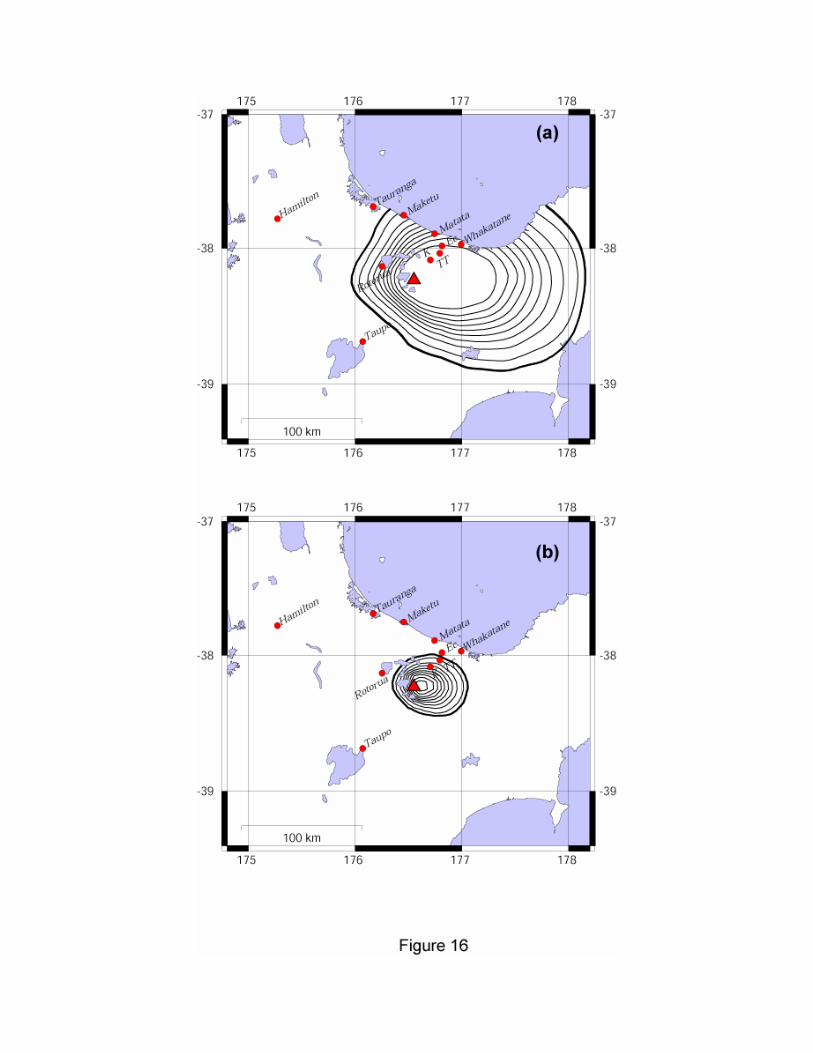
If Tarawera Volcano generates a multi-phase eruption characterized by 10

eruptive episodes with plumes ranging between 14 and 26 km (MES maps; Runs 8 in

Table 1), the main populated towns northeast of the volcano are likely to receive enough

tephra fall to cause damage to agriculture (75-100%; Fig. 16a). Rotorua and Maketu

(northwest of the volcano) are also likely to experience damage to agriculture (15-40%;

Fig. 16a). Some towns on the northeast (i.e. Kawerau and Te Teko) of the volcano are

likely to experience collapse of the weakest buildings (15-50%; Fig. 16b). Kawerau is

also likely to experience collapse of even the strongest buildings (5%; the map for 600 kg

m-2 is not shown as this specific mass loading would only marginally affect Kawerau).

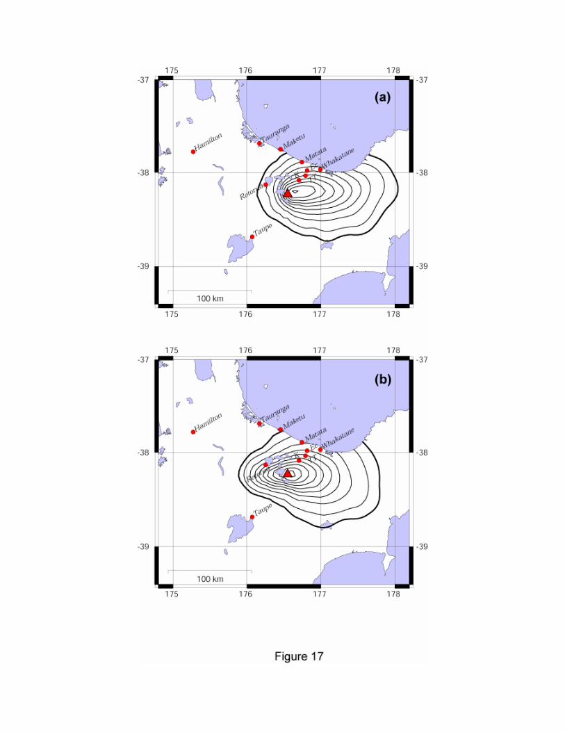
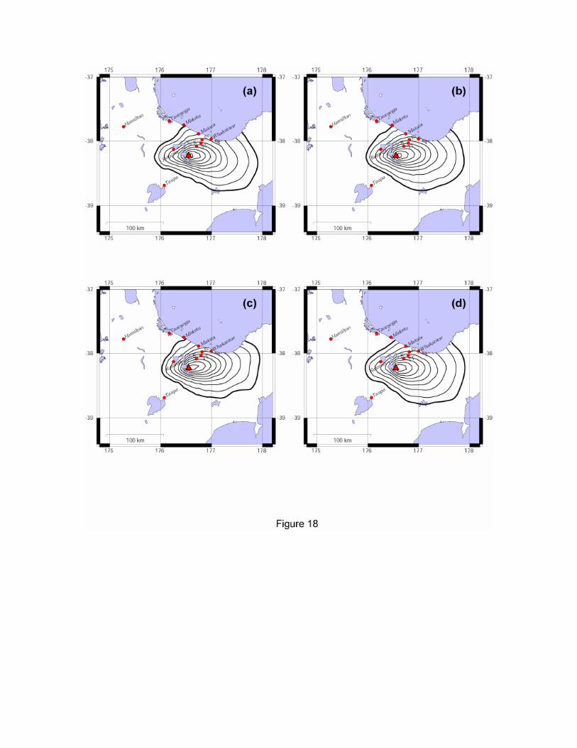
4.2.3 Seasonal variations and climate fluctuations

(Runs 9 to 14 in Table 1)

The 1996-1998 wind data show that winds up to 25 km above sea level in the

North Island of New Zealand mainly blow to the northeast-east-southeast (Fig. 11a and

12a). During the austral spring-summer wind can also blow to the northwest-west-

southwest. However, the ULS probability maps computed for a threshold of 30 kg m-2,

both for the austral winter (June-August; i.e. wind only to the northeast-east-southeast;

Runs 9 in Table 1) and the austral spring-summer (September-March; i.e. some winds

also to the northwest-west-southwest; Runs 10 in Table 1) do not diverge significantly

(Fig. 17). If Tarawera Volcano produces a 26-km-high plume, Rotorua is more likely to

experience damage to agriculture between September-March (about 40%; Fig. 17b),

whereas the probability of reaching the threshold of damage to agriculture does not vary

significantly for the populated towns northeast of the volcano (20-60%; Fig. 17).

As also mentioned above, the North Island of New Zealand is located in the mid-

latitudes, and therefore is not significantly affected by "El Niño Southern Oscillation

28

(ENSO) phenomenon", the major systematic global climate fluctuation that occurs at the

time of an ocean warming event. However, in order to have a comprehensive wind

analysis, we have chosen 3 years characterized by the main climate conditions: January

1996 to March 1997 (neutral conditions); April 1997 to May 1998 (strong El Niño); after

May 1998 (La Niña). ULS probability maps computed using only wind data from 1996

(i.e. neutral conditions; Runs 11 in Table 1) and wind data only from 1997-1998 (i.e.

ENSO conditions; Runs 12 in Table 1) do not show significant differences (Figs 18a and

18b). Also ULS probability maps computed using only wind data characterized by strong

El Niño (i.e. April 1997 to May 1998; Runs 13 in Table 1) and by La Niña (i.e. after May

1998; Runs 14 in Table 1) do not show significant differences (Figs 18c and 18d). As a

conclusion, the winter times are the times when the area west and north-west of Tarawera

would be affected the least by a Kaharoa-type eruption, regardless ENSO phenomenon.

5. Discussion TEPHRA results from the combination of different theories and modeling

approaches, representing a first step towards the integration of two main classes of

tephra-fall dispersal models developed during the last two decades: (i) advection-

diffusion models [Armienti et al., 1988; Bonadonna et al., 2002a; Connor et al., 2001;

Glaze and Self, 1991; Macedonio et al., 1988; Suzuki, 1983] and (ii) models describing

large-eddy sedimentation from plume margins combined with gravity-driven intrusion of

the volcanic current at the neutral buoyancy level [Bonadonna and Phillips, 2003; Bursik

et al., 1992a; Bursik et al., 1992b; Ernst et al., 1996; Koyaguchi and Ohno, 2001a;

Sparks et al., 1992].

Hazard assessments are typically done using advection-diffusion models, which are

mostly empirical but that are designed to compile mass/area and probability maps

[Barberi et al., 1990; Bonadonna et al., 2002a; Hill et al., 1998]. The models from the

second class are based on classic plume theory and have mainly focused on thoroughly

describing the tephra-fall dynamics but have not been used to compile 2D maps due to

the more complex theory involved. Eventually these two classes should merge, and

TEPHRA can be identified as a first step towards this direction. As an example,

29

TEPHRA describes an instantaneous release of particles from the eruptive source, typical

of advection-diffusion models [e.g. Armienti et al., 1988], implemented by the horizontal

diffusion time, 'it , that accounts for the change in width of the plume as a function of

height (eq. (7)), derived from classic plume theory [Morton et al., 1956]. This results in

smaller atmospheric diffusion coefficients (e.g. diffusion coefficient = 200-600 m2 s-1),

given that diffusion coefficients in advection-diffusion models typically account also for

the horizontal diffusion of the plume (e.g. diffusion coefficient = 3000 m2 s-1, Vesuvius

[Macedonio et al., 1988]; 6000 m2 s-1, Ruapehu [Hurst and Turner, 1999]; 2700 m2 s-1,

Montserrat [Bonadonna et al., 2002a]). TEPHRA also better describes tephra fall

accounting for the variation of particle Reynold’s Number along the particle trajectory.

TEPHRA is also one of the first dispersal models to account for the variation of

diffusion law with particle size: (i) linear-diffusion for coarse particles and (ii) power-law

diffusion for fine particles. Atmospheric turbulent diffusion is neglected by most models

based on the gravitional spreading of plumes [Bonadonna and Phillips, 2003; Bursik et

al., 1992b; Sparks et al., 1992], whereas advection-diffusion models typically account for

diffusion of coarse particles only [Armienti et al., 1988; Bonadonna et al., 2002a; Connor

et al., 2001], even though the diffusion is thought to be particularly significant for settling

of ash-sized particles [Suzuki, 1983; Bursik et al., 1992a]. However, the cut off for

diffusion-law decoupling is not yet well characterised and can be only determined

empirically (e.g. 1080 s for the distal tephra-fall from the 17 June 1996 eruption of

Ruapehu; Fig. 7).

TEPHRA can also account for sedimentation from strong and weak plumes varying

the mass-distribution factor . Large values of place more mass, proportionally, at

the top of the volcanic plume, simulating more powerful eruptions (Fig. 4). Sensitivity

tests done on selected Ruapehu samples show that a weak plume can be simulated using

small values of (Runs 1-2; Figs 7 and 8). Distal deposit from this eruption shows a

larger best-fit value of than the total deposit, as expected. Unfortunately though, a good

data set from a strong-plume deposit is not available to investigate the actual best-fit

value for strong plumes. Sensitivity tests done on selected Ruapehu samples show that

30

variations of values result in significant variations of mf. As an example an increase of

about 100% of the value characterized by the minimum mf, results in a variation of

about 3% of mf for both the total and the distal data sets of the Ruapehu deposit (Fig. 7c).

Sensitivity tests also show that varying the fall-time cut off does not result in a significant

variation of mf, whereas varying the diffusion coefficient of about 100% of the initial

value has produced a maximum variation of about 45% of the initial mf value (i.e. total

data set) (Fig. 7a and 7b). As a conclusion, values for diffusion coefficient and need to

be selected more carefully than the fall-time cut off.

Model implementations were made possible by the parallelization of the code. In

fact, most advection-diffusion models run on single processors and used to compile

probability maps require several assumptions in order to reduce the number of calculation

and speed up the execution times (e.g. uniform wind field; constant particle-settling

velocity; single diffusivity law; constant particle density). TEPHRA does not require

many assumptions because the execution times are speed up by the use of multiple

processors. Geoscientific problems can be made “parallel” at a number of levels. The use

of TEPHRA for hazard assessment can be defined as “embarrassingly parallel” because

the same calculations are performed independently for a large number of input

parameters and for a large number of grid points. Computation is greatly accelerated by

dividing the grid points among several different computers and simultaneously

performing the calculations on each. Since the solution at one grid point does not depend

on the solution at any other grid point, this grid decomposition is straightforward. This

type of parallel code is called a "single program - multiple data" model (SPMD), because

multiple instances of the same computer code run on multiple processors. In a well-

implemented SPMD problem, computational speed scales with the number of nodes used.

Parallelization of the code not only allows the implementation of the model but

also allows a fully probabilistic approach to tephra-fall hazard. A stochastic parameter

sampling is used to identify a range of input parameters for the physical model (i.e.

column height; eruption duration; mass distribution parameter; grainsize distribution;

eruptive vent; clast exit velocity). This is important because sometimes different eruptive

31

scenarios need to be investigated but also because often these parameters are not well

known but can be sampled from probability density functions. The more simulations are

done the better the full range of possible outcomes is understood, making the problem

inherently parallel because the exact same computations are performed many times on

different input data.

The tephra-fall hazard assessment of Tarawera Volcano represents a typical

situation: Tarawera did not produce several historical eruptions and therefore the data

available for model calibration and for the identification of input parameters and eruptive

scenarios are not very accurate. Furthermore, Tarawera is characterized by multiple

eruptive vents and most eruptions from this volcano are characterized by multiple

eruptive phases (e.g. AD 1305 Kaharoa eruption; AD 1886 eruption). Therefore our

hazard assessment was based on a fully stochastic sampling of input parameters because

most of these parameters are not very well known (i.e. grainsize; clast exit velocity; mass

distribution parameter; Fig. 6) but also because different eruptive scenarios need to be

investigated (i.e. eruptive vent; plume height; eruption duration; Fig. 5).

A probabilistic approach is also used to forecast a range of possible outcomes (i.e.

hazard curves and probability maps), so that the probability of exceeding certain

hazardous tephra-fall accumulations can be investigated for different eruptive scenarios

and a wide area around the eruptive vent (Fig. 13-18). The calculation of tephra-fall

accumulation on a grid is also inherently parallel because the exact same computations

are performed many times for different grid points.

TEPHRA describes the particle transport at discrete atmospheric level (e.g. 1 km)

accounting for settling-velocity variations (based on particle Reynold’s Number

variation) and wind variations (i.e. direction and velocity). The accuracy of the resulting

hazard assessment is strictly related to the accuracy and number of wind profiles used and

weather fluctuations analyzed. The detailed gridded zonal and meridional wind fields

downloaded from the NCEP Reanalysis project allowed a full hazard assessment

32

including specific seasonal assessments (Fig. 17) and assessments for particular climate

conditions (e.g. ENSO phenomenon; Fig. 18).

A good statistical study of wind profiles also help constrain the occurrence time

of a given eruption. As an example, Fig. 11 shows that winds below 25 km above sea

level around the Tarawera Volcanic Complex blow between N and S with main direction

to the E, and winds above 25 km blow between W and E with main direction to the N.

Fig. 12 also shows that winds are more likely to blow to the W and N during September

through March. Given that the 5 Kaharoa units dispersed to the N and NW were produced

consecutively and by plumes smaller than 25 km (i.e. Units H, I, J, K and L; plume height

between 16-24 km [Sahetapy-Engel, 2002]), it is likely that Units H to L were produced

during the same austral spring-summer. However, Units A to G were dispersed to the SE

and therefore it is more difficult to estimate the corresponding occurrence time, given that

winds can blow to the SE during the whole year (Fig. 12). Our probabilistic analysis for

the ENSO phenomenon also indicates that the unusual wind conditions that produced the

Kaharoa tephra-fall dispersal cannot be explained as en effect of El Niño or La Niña

climate fluctuations (Fig. 18). Therefore, based on purely tephra-fall dispersal

considerations, we can conclude the whole Kaharoa eruption could have occurred during

an austral spring-summer or at least 5 consecutive units are very likely to have occurred

during the same austral spring-summer. However, magma-chamber dynamics and

volcanic edifice geometry should also be considered in order to assess magma-chamber

recharging times and the times required to establish certain eruptive conditions [Melnik,

2000; Pinel and Jaupart, 2003].

6.1 Model caveats

TEPHRA represents a great implementation of the existing advection-diffusion

models of tephra-fall dispersal. However, there are still some parameters and processes

that need to be investigated and studied in more details. First of all, the mass distribution

within the eruptive plume is controlled by the factor and by the determination of the

particle-settling velocity within the plume and the plume vertical velocity. The factor

allows to switch between sedimentation from strong plumes and sedimentation from

33

weak plumes, but is an empirical parameter not supported by a robust theory. Moreover,

the determination of particle-settling velocity within the plume and plume vertical

velocity is very complex and TEPHRA still uses empirical parameters based on the

theory from Suzuki [1983]. A more thorough model is needed to describe the plume

dynamics.

A further implementation of TEPHRA could be describing the effects of

aggregation processes and particle shape on tephra-fall dispersal. Aggregation processes

were not accounted for in our assessment because no particle-aggregation data are

available for the Kaharoa eruption. A reliable parameterization that can describe

aggregation processes during tephra fall even when direct observations are not possible

would help describe tephra-fall features also from those volcanoes that do not erupt very

frequently and therefore do not provide detailed information of their eruptive processes.

A simple parameterization of the effect of particle shape on particle-settling velocity

would also significantly improve the description of tephra-fall dispersal. Unfortunately,

modeling settling velocities without the assumption of spherical particles is still very

complex [Chhabra et al., 1999]. Nonetheless, the stochastic sampling of grainsize

parameters used in our assessment can at least provide a complete analysis regardless the

lack of reliable observations due to the difficulties of studying an old tephra-fall deposit.

Advection-diffusion models are typically characterized by particle release at

time=0, and therefore do not account for wind-profile variations with time that can

significantly affect long-lasting eruptions. Another important implementation of

advection-diffusion models in the frame of forecasting tephra-fall dispersal for hazard

assessment would be including the time factor for the simulation of tephra fall.

Finally, reliable datasets from powerful eruptions are needed to calibrate

advection-diffusion models more accurately. Our calibration was based on one very good

dataset from a weak subplinian plume. In order to have more reliable models for tephra-

fall dispersal that can provide reliable hazard assessments, we need more datasets

complete with direct observations of tephra-fall processes and accurate data processing.

34

7. Conclusions

A new advection-diffusion model, TEPHRA, was developed from the

combination of several theories and modeling approaches to provide an efficient and

reliable tool for hazard assessment of tephra fall from weak and strong plumes. After a

careful analysis of the model, we can conclude that:

1. the main implementations of TEPHRA are represented by: (i)

parallelization of the advection-diffusion code, (ii) fully probabilistic assessment of

input and output parameters and (iii) more robust algorithm.

2. parallel modeling is the ideal computational approach for hazard

assessment as, given the short computing times, it increases the hazard map resolution

and reliability because calculations can be done on more points and because the

physical models can be based on a more robust algorithm;

3. the short computing times that characterize parallel modeling also allow a

fully probabilistic assessment based on (i) a stochastic sampling of input parameters

and (ii) a probabilistic analysis of possible outcomes;

4. the main implementations of the advection-diffusion algorithm are: (i)

grainsize dependent diffusion law, (ii) particle-settling velocities that account for

Reynold’s Number variations along the particle trajectory and (iii) use of the mass-

distribution factor to simulate sedimentation from strong as well as weak plumes

(i.e. using large and small values of respectively);

5. output results are sensitive to the choice of diffusion coefficient and

values and less sensitive to the choice of fall-time cut off.

A combination of observations from the AD 1305 Kaharoa eruption and model

simulations enabled us to evaluate probabilistically the accumulations and effects in

different areas of the North Island (NZ) of tephra fall produced by Tarawera Volcano and

based on the assumption of three different eruptive scenarios: (i) Upper Limit Scenario (1

eruptive episode happening with a 26-km-high plume), (ii) Eruption Range Scenario (1

eruptive episode happening with a plume in the range 14-26 km) and (iii) Multiple

35

Eruption Scenario (10 eruptive episodes with plumes in the range 14-26 km). On the

basis of our tephra-fall hazard assessment we can also conclude that:

6. due to the prevailing winds below 25 km above sea level blowing between

N and S with main direction to the E, the areas W and S of the Tarawera Volcanic

Complex are likely to receive little tephra fall from a Kaharoa-type eruption.

Therefore key cities such as Tauranga, Hamilton and Auckland are relatively safe

from hazardous accumulation of tephra fall;

7. the most affected localities are key towns NE of Tarawera that are likely

to experience damage to vegetation in the case of ULS, ERS and MES and partial

collapse of building in the case of ULS and MES;

8. detailed wind analysis shows that the dispersal of tephra fall from

Tarawera Volcano is not significantly affected by El Niño or La Niña fluctuations,

whereas is slightly affected by seasonal variations, with the area immediately west of

the volcano being more likely to receive tephra fall during the austral spring-summer;

9. based on purely tephra-fall dispersal considerations, the whole Kaharoa

eruption might have occurred during an austral spring-summer or at least 5

consecutive units are very likely to have occurred during the same austral spring-

summer (i.e. Units H to L).

Acknowledgments

Many thanks to Steve Sahetapy-Engel for his continuous support and sharing of his

experience and knowledge of the AD 1305 Kaharoa eruption. NCEP Reanalysis data

were provided by the NOAA-CIRES Climate Diagnostics Center, Boulder, Colorado,

USA, from their Web site at http://www.cdc.noaa.gov/. This research was funded by a

subcontract from the Foundation for Research, Science and Technology via Professor

J.W. Cole and the University of Canterbury (New Zealand).

36

References

Armienti, P., G. Macedonio, and M.T. Pareschi, A numerical-model for simulation of tephra transport and deposition - applications to May 18, 1980, Mount-St-Helens eruption, Journal of Geophysical Research, 93 (B6), 6463-6476, 1988.

Barberi, F., G. Macedonio, M.T. Pareschi, and R. Santacroce, Mapping the tephra fallout risk: an example from Vesuvius, Italy, Nature, 344, 142-144, 1990.

Blong, R., The Rabaul Eruption, 1994, Australian Geographer, 25 (2), 186-190, 1994. Blong, R.J., Volcanic Hazards. A sourcebook on the effects of eruptions, 424 pp.,

Academic Press, Sidney, 1984. Bonadonna, C., Models of tephra dispersal, Ph.D. thesis, University of Bristol, Bristol,

2001.Bonadonna, C., G.G.J. Ernst, and R.S.J. Sparks, Thickness variations and volume

estimates of tephra fall deposits: the importance of particle Reynolds number, Journal of Volcanology and Geothermal Research, 81 (3-4), 173-187, 1998.

Bonadonna, C., G. Macedonio, and R.S.J. Sparks, Numerical modelling of tephra fallout associated with dome collapses and Vulcanian explosions: application to hazard assessment on Montserrat, in The eruption of Soufrière Hills Volcano, Montserrat, from 1995 to 1999, edited by T.H. Druitt, and B.P. Kokelaar, pp. 517-537, Geological Society, London, Memoir, 2002a.

Bonadonna, C., and J.C. Phillips, Sedimentation from strong volcanic plumes, Journal of Geophysical Research, 108 (B7), 2340-2368, 2003.

Bursik, M.I., S.N. Carey, and R.S.J. Sparks, A gravity current model for the May 18, 1980 Mount-St-Helens plume, Geophysical Research Letters, 19 (16), 1663-1666, 1992a.

Bursik, M.I., R.S.J. Sparks, J.S. Gilbert, and S.N. Carey, Sedimentation of tephra by volcanic plumes: I. Theory and its comparison with a study of the Fogo A plinian deposit, Sao Miguel (Azores), Bulletin of Volcanology, 54, 329-344, 1992b.

Carey, S., and H. Sigurdsson, The intensity of Plinian eruptions, Bulletin of Volcanology,51, 28-40, 1989.

Carey, S.N., and H. Sigurdsson, Influence of particle aggregation on deposition of distal tephra from the May 18, 1980, eruption of Mount St-Helens volcano, Journal of Geophysical Research, 87 (B8), 7061-7072, 1982.

Carey, S.N., and R.S.J. Sparks, Quantitative models of the fallout and dispersal of tephra from volcanic eruption columns, Bulletin of Volcanology, 48, 109-125, 1986.

Chhabra, R.P., L. Agarwal, and N.K. Sinha, Drag on non-spherical particles: an evaluation of available methods, Powder Technology, 101 (3), 288-295, 1999.

Chung, M.R., The eruption of Nevado del Ruiz Volcano, Colombia, South America (November 13,1985), in Natural Disaster Studies, edited by N.R. Council, pp. 109, National Academy Press, Washington, D.C., 1991.

Cole, J.W., Structure and eruptive history of Tarawera Volcanic Complex, New Zealand Journal of Geology and Geophysics, 13, 879-902, 1970.

Coltelli, M., M. Pompilio, P. Del Carlo, S. Calvari, S. Pannucci, and V. Scribano, Etna. Eruptive activity, in Data related to eruptive activity, unrest phenomena and other observations on the Italian active volcanoes – Geophysical monitoring of

37

the Italian active volcanoes 1993-1995, edited by P. Gasparini, pp. 141-148, Acta Vulcanologica, 1998.

Connor, C.B., B.E. Hill, B. Winfrey, N.M. Franklin, and P.C. La Femina, Estimation of volcanic hazards from tephra fallout, Natural Hazards Review, 2 (1), 33-42, 2001.

Di Vito, M.A., R. Isaia, G. Orsi, J. Southon, M. D'Antonio, S. de Vita, L. Pappalardo, and M. Piochi, Volcanism and deformation since 12,000 years at the Campi Flegrei caldera (Italy), Journal of Volcanology and Geothermal Research, 91 (2-4), 221-246, 1999.

Ernst, G.G.J., R.S.J. Sparks, S.N. Carey, and M.I. Bursik, Sedimentation from turbulent jets and plumes, Journal of Geophysical Research-Solid Earth, 101 (B3), 5575-5589, 1996.

Fedotov, S.A., S.T. Balesta, V.N. Dvigalo, A.A. Razina, G.B. Flerov, and A.M. Chirkov, New Tolbachik Volcanoes, in Active volcanoes of Kamchatka, edited by O.M. Vanyukova, pp. 302, Nauka Publisher, Moscow, 1991.

Geist, A., A. Beguelin, J. Donagarra, W. Jaing, R. Mancheck, and V. Sunderam, PVM:Parallel Virtual Machine - a User's Guide and Tutorial for Networked Parallel Computing., 279 pp., The MIT Press, Cambridge, Ma, 1997.

Glaze, L.S., and S. Self, Ashfall dispersal for the 16 September 1986, eruption of Lascar, Chile, calculated by a turbulent-diffusion model, Geophysical Research Letters,18 (7), 1237-1240, 1991.

Hanna, S.R., G.A. Briggs, and R.P. Hosker, Handbook on atmospheric diffusion, 102 pp., Technical Information Center (U.S. Department of Energy), 1982.

Hildreth, W., and R.E. Drake, Volcano Quizapu, Chilean Andes, Bulletin of Volcanology,54, 93-125, 1992.

Hill, B.E., C.B. Connor, M.S. Jarzemba, P.C. La Femina, M. Navarro, and W. Strauch, 1995 eruptions of Cerro Negro volcano, Nicaragua, and risk assessment for future eruptions, Geological Society of America Bulletin, 110 (10), 1231-1241, 1998.

Hurst, A.W., and R. Turner, Performance of the program ASHFALL for forecasting ashfall during the 1995 and 1996 eruptions of Ruapehu volcano, New Zealand Journal of Geology and Geophysics, 42 (4), 615-622, 1999.

Inman, D.L., Measures for describing the size distribution of sediments, Journal of Sedimentary Petrology, 22, 125-145, 1952.

Iverson, R.M., S.P. Schilling, and J.W. Vallance, Objective delineation of lahar-inundation hazard zones, Geological Society of America Bulletin, 110, 972-984, 1998.

Kalnay, E., M. Kanamitsu, R. Kistler, W. Collins, D. Deaven, L. Gandin, M. Iredell, S. Saha, G. White, J. Woollen, Y. Zhu, M. Chelliah, W. Ebisuzaki, W. Higgins, J. Janowiak, K.C. Mo, C. Ropelewski, J. Wang, A. Leetmaa, R. Reynolds, R. Jenne, and D. Joseph, The NCEP/NCAR 40-year reanalysis project, Bulletin of the American Meteorological Society, 77 (3), 437-471, 1996.

Keam, R.F., Tarawera: the volcanic eruption of 1886, 472 pp., R.F. Keam, Auckland, 1988.

Kokelaar, B.P., Setting, chronology and consequences of the eruption of Soufrière Hills Volcano, Montserrat (1995-1999), in The eruption of Soufrière Hills Volcano, Montserrat, from 1995 to 1999, edited by T.H. Druitt, and B.P. Kokelaar, Geological Society, London, Memoir, 2002.

38

Koyaguchi, T., and M. Ohno, Reconstruction of eruption column dynamics on the basis of grain size of tephra fall deposits. 1. Methods, Journal of Geophysical Research,106 (B4), 6499-6512, 2001a.

Kunii, D., and O. Levenspiel, Fluidisation Engineering, Wiley and Sons, New York, 1969.

Lacroix, A., La Montagne Pelée et ses eruptions, Masson, Paris, 1904. Macedonio, G., M.T. Pareschi, and R. Santacroce, A numerical simulation of the Plinian

fall phase of 79 AD eruption of Vesuvius, Journal of Geophysical Research-Solid Earth and Planets, 93 (B12), 14817-14827, 1988.

Maulucci Vivolo, F.P., Lettere di Plinio il Giovane a Tacito sull'eruzione del Vesuvio (da C. Plini Caecili Secundi Epistularum libri decem), pp. 39, Bastogi Editrice Italiana, Foggia, 1994.

Melnik, O., Dynamics of two-phase conduit flow of high-viscosity gas-saturated magma: large variations of sustained explosive eruption intensity, Bulletin of Volcanology,62 (3), 153-170, 2000.

Morton, B., G.L. Taylor, and J.S. Turner, Turbulent gravitational convection from maintained and instantaneous source, Proceedings of the Royal Society, 234, 1-23, 1956.

Nairn, I.A., Sheet V16AC-Tarawera. Geological map of New Zealand 1:50000, Department of Scientific and Industrial Research, Wellinghton, 1989.

Nairn, I.A., S. Self, J.W. Cole, G.S. Leonard, and C. Scutter, Distribution, stratigraphy, and history of proximal deposits from the c. AD 1305 Kaharoa eruptive episode at Tarawera Volcano, New Zealand, New Zealand Journal of Geology and Geophysics, 44, 467-484, 2001.

Newhall, C.G., and R.P. Hoblitt, Constructing event trees for volcanic crises, Bulletin of Volcanology, 64, 3-20, 2002.

Pasquill, F., Atmospheric Diffusion, John Wiley & Sons, Chichester, 1974. Pinel, V., and C. Jaupart, Magma chamber behavior beneath a volcanic edifice, Journal

of Geophysical Research-Solid Earth, 108 (B2), 2003. Prata, A.J., and I.F. Grant, Retrieval of microphysical and morphological properties of

volcanic ash plumes from satellite data: Application to Mt Ruapehu, New Zealand, Quarterly Journal of the Royal Meteorological Society, 127 (576), 2153-2179, 2001.

Pyle, D.M., The thickness, volume and grainsize of tephra fall deposits, Bulletin of Volcanology, 51 (1), 1-15, 1989.

Sahetapy-Engel, S., Tephra fall deposit of the AD 1305 eruption of Tarawera, New Zealand: reconstruction of eruption dynamics, Master thesis, University of Hawaii, Honolulu, 2002.

Sparks, R.S.J., The dimensions and dynamics of volcanic eruption colums, Bulletin of Volcanology, 48, 3-15, 1986.

Sparks, R.S.J., M.I. Bursik, G.J. Ablay, R.M.E. Thomas, and S.N. Carey, Sedimentation of tephra by volcanic plumes .2. Controls on thickness and grain-size variations of tephra fall deposits, Bulletin of Volcanology, 54 (8), 685-695, 1992.

Sparks, R.S.J., M.I. Bursik, S.N. Carey, J.S. Gilbert, L.S. Glaze, H. Sigurdsson, and A.W. Woods, Volcanic Plumes, 574 pp., John Wiley & Sons, Chichester, 1997.

39

Sparks, R.S.J., and G.P.L. Walker, The significance of vitric-enriched air-fall ashes associated with crystal-enriched ignimbrites, Journal of Volcanology and Geothermal Research, 2, 329-341, 1977.

Sparks, R.S.J., and L. Wilson, Explosive volcanic eruptions: V. Observations of plume dynamics during the 1979 Soufrière eruption, St. Vincent, Geophysical Journal of the Royal Astronomical Society, 69, 551-570, 1982.

Sparks, R.S.J., L. Wilson, and H. Sigurdsson, The pyroclastic deposits of the 1875 eruption of Askja, Iceland, Philosophical Transaction of the Royal Society of London, 229, 241-273, 1981.

Sparks, R.S.J., and S.R. Young, The eruption of Soufrière Hills Volcano, Montserrat (1995-1998): overview of scientific results, in The eruption of Soufrière Hills Volcano, Montserrat, from 1995 to 1999, edited by T.H. Druitt, and B.P. Kokelaar, Geological Society, London, Memoir, 2002.

Sterling, T.L., J. Salmon, D.J. Becker, and D.F. Savarese, How to build a Beowulf - a Guide to implementation and application of PC clusters, 239 pp., The MIT Press, Cambridge, Ma, 1999.

Stirling, M.W., and C.J.N. Wilson, Development of a volcanic hazard model for New Zealand: first approaches from the methods of probabilistic seismic hazard analysis, Bulletin of the New Zealand Society for Earthquake engineering, 35 (4), 266-277, 2002.

Suzuki, T., A theoretical model for dispersion of tephra, in Arc Volcanism, Physics and Tectonics, edited by D. Shimozuru, and I. Yokoyama, pp. 95-113, Terra Scientific Publishing Company (TERRAPUB), Tokyo, 1983.

Wadge, G., P. Jackson, S.M. Bower, A.W. Woods, and E. Calder, Computer simulations of pyroclastic flows from dome collapse, Geophysical Research Letters, 25 (19), 3677-3680, 1998.

Walker, G.P.L., The Taupo Pumice: product of the most powerful known (Ultraplinian) eruption?, Journal of Volcanology and Geothermal Research, 8, 69-94, 1980.

Walker, G.P.L., The Waimihia and Hatepe plinian deposits from the rhyolitic Taupo Volcanic Centre, New Zealand Journal of Geology and Geophysics, 24, 305-324, 1981.

Walker, G.P.L., S. Self, and L. Wilson, Tarawera, 1886, New Zealand - A basaltic Plinian fissure eruption, Journal of Volcanology and Geothermal Research, 21,61-78, 1984.

Williams, H., Volcanoes of the Paricutin Region, USGS Bulletin, 965 (B), 165-275, 1950. Wilson, L., and T.C. Huang, The influence of shape on the atmospheric settling velocity

of volcanic ash particles, Earth and Planetary Sciences Letters, 44, 311-324, 1979.

Woo, G., The mathematics of natural catastrophes, 292 pp., Imperial College Press, London, 2000.

Woods, A.W., The fluid-dynamics and thermodynamics of eruption columns, Bulletin of Volcanology, 50 (3), 169-193, 1988.

Woods, W., The dynamics of explosive volcanic eruptions, Review of Geophysics (AGU),33 (4), 495-530, 1995.

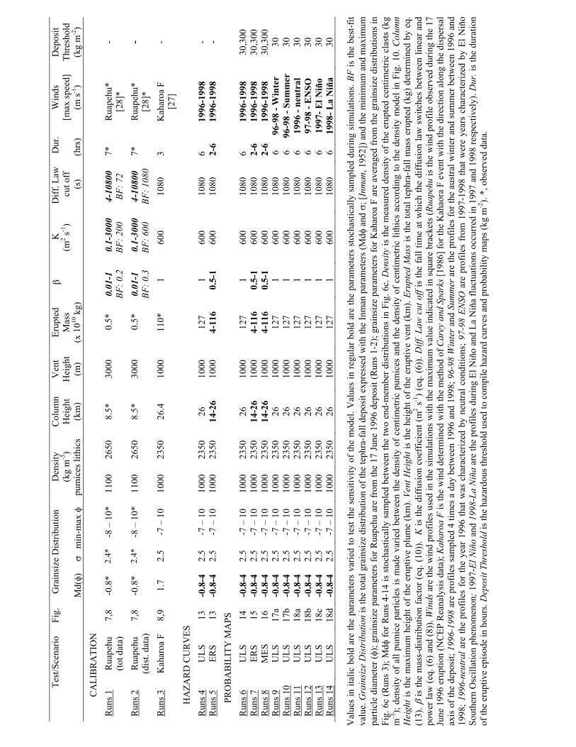
Te

st/S

cena

rio

Fig.

G

rain

size

Dis

tribu

tion

Md(

)m

in-m

ax

Den

sity

(k

g m

-3)

pum

ices

lith

ics

Col

umn

Hei

ght

(km

)

Ven

tH

eigh

t (m

)

Erup

ted

Mas

s(x

1010

kg)

K

(m2 s-1

) D

iff. L

aw

cut

off

(

s)

Dur

.

(hrs

)

Win

ds

[max

spee

d]

(m s-1

)

Dep

osit

Thre

shol

d (k

g m

-2)

C

ALI

BR

ATI

ON

Run

s 1

Rua

pehu

(to

t dat

a)

7,8

-0.8

* 2.

4*-8

– 1

0*

1100

26

50

8.5*

30

00

0

.5*

0.01

-1

BF: 0

.2 0

.1-3

000

BF: 2

00

4-10

800

BF: 7

27*

R

uape

hu*

[28]

* -

Run

s 2

Rua

pehu

(d

ist.

data

) 7,

8 -0

.8*

2.4*

-8 –

10*

11

00

2650

8.

5*

3000

0.5

* 0.

01-1

BF

: 0.3

0.1

-300

0 BF

: 600

4-10

800

BF: 1

080

7*R

uape

hu*

[28]

*-

Run

s 3

Kah

aroa

F

8,9

1.7

2.5

-7 –

10

1000

23

50

26.4

10

00

110*

1

600

1080

3

Kah

aroa

F

[27]

-

H

AZA

RD

CU

RV

ES

Run

s 4

ULS

13

-0

.8-4

2.

5 -7

– 1

0 10

00

2350

26

10

00

127

1 60

010

80

6 19

96-1

998

-R

uns 5

ER

S 13

-0

.8-4

2.

5 -7

– 1

0 10

00

2350

14

-26

1000

4-

116

0.5-

1 60

010

80

2-6

1996

-199

8 -

PR

OB

AB

ILIT

Y M

APS

Run

s 6

ULS

14

-0

.8-4

2.

5 -7

– 1

0 10

00

2350

26

10

00

127

1 60

010

80

6 19

96-1

998

30,3

00

Run

s 7

ERS

15

-0.8

-4

2.5

-7 –

10

1000

23

50

14-2

6 10

004-

116

0.5-

1 60

010

80

2-6

1996

-199

8 30

,300

R

uns 8

M

ES

16

-0.8

-4

2.5

-7 –

10

1000

23

50

14-2

6 10

004-

116

0.5-

1 60

010

80

2-6

1996

-199

8 30

,300

R

uns 9

U

LS

17a

-0.8

-4

2.5

-7 –

10

1000

23

50

26

1000

127

1 60

010

80

6 96

-98

- Win

ter

30R

uns 1

0 U

LS

17b

-0.8

-4

2.5

-7 –

10

1000

23

50

26

1000

127

1 60

010

80

696

-98

- Sum

mer

30

Run

s 11

ULS

18

a -0

.8-4

2.

5 -7

– 1

0 10

00

2350

26

10

0012

7 1

600

1080

6

1996

- ne

utra

l 30

Run

s 12

ULS

18

b -0

.8-4

2.

5 -7

– 1

0 10

00

2350

26

10

0012

7 1

600

1080

6

97-9

8 - E

NSO

30

Run

s 13

ULS

18

c -0

.8-4

2.

5 -7

– 1

0 10

00

2350

26

10

0012

7 1

600

1080

6

1997

- El N

iño

30R

uns 1

4 U

LS

18d

-0.8

-4

2.5

-7 –

10

1000

23

50

26

1000

127

1 60

010

80

619

98- L

a N

iña

30

Val

ues

in it

alic

bol

d ar

e th

e pa

ram

eter

s va

ried

to te

st th

e se

nsiti

vity

of t

he m

odel

. Val

ues

in re

gula

r bol

d ar

e th

e pa

ram

eter

s st

ocha

stic

ally

sam

pled

dur

ing

sim

ulat

ions

. BF

is th

e be

st-f

it va

lue.

Gra

insi

ze D

istr

ibut

ion

is th

e to

tal g

rain

size

dis

tribu

tion

of th

e te

phra

-fal

l dep

osit

expr

esse

d w

ith th

e In

man

par

amet

ers (

Md

and

[Inm

an, 1

952]

) and

the

min

imum

and

max

imum

pa

rticl

e di

amet

er (

); gr

ains

ize

para

met

ers

for R

uape

hu a

re fr

om th

e 17

Jun

e 19

96 d

epos

it (R

uns

1-2)

; gra

insi

ze p

aram

eter

s fo

r Kah

aroa

F a

re a

vera

ged

from

the

grai

nsiz

e di

strib

utio

ns in

Fi

g. 6

c (R

uns

3); M

d fo

r Run

s 4-

14 is

sto

chas

tical

ly s

ampl

ed b

etw

een

the

two

end-

mem

ber d

istri

butio

ns in

Fig

. 6c.

Den

sity

is th

e m

easu

red

dens

ity o

f the

eru

pted

cen

timet

ric c

last

s (k

g m

-3);

dens

ity o

f all

pum

ice

parti

cles

is m

ade

varie

d be

twee

n th

e de

nsity

of c

entim

etric

pum

ices

and

the

dens

ity o

f cen

timet

ric li

thic

s ac

cord

ing

to th

e de

nsity

mod

el in

Fig

. 10.

Col

umn

Hei

ght i

s th

e m

axim

um h

eigh

t of t

he e

rupt

ive

plum

e (k

m).

Vent

Hei

ght i

s th

e he

ight

of t

he e

rupt

ive

vent

(km

). Er

upte

d M

ass

is th

e to

tal t

ephr

a-fa

ll m

ass

erup

ted

(kg)

det

erm

ined

by

eq.

(13)

. is

the

mas

s-di

strib

utio

n fa

ctor

(eq.

(10)

). K

is th

e di

ffus

ion

coef

ficie

nt (m

2 s-1

) (eq

. (6)

). D

iff. L

aw c

ut o

ff is

the

fall

time

at w

hich

the

diff

usio

n la

w s

witc

hes

betw

een

linea

r and

po

wer

law

(eq.

(6) a

nd (8

)). W

inds

are

the

win

d pr

ofile

s us

ed in

the

sim

ulat

ions

with

the

max

imum

val

ue in

dica

ted

in s

quar

e br

acke

ts (R

uape

hu is

the

win

d pr

ofile

obs

erve

d du

ring

the

17

June

199

6 er

uptio

n (N

CEP

Rea

naly

sis d

ata)

; Kah

aroa

F is

the

win

d de

term

ined

with

the

met

hod

of C

arey

and

Spa

rks [

1986

] for

the

Kah

aora

F e

vent

with

the

dire

ctio

n al

ong

the

disp

ersa

l ax

is o

f the

dep

osit;

199

6-19

98 a

re p

rofil

es s

ampl

ed 4

tim

es a

day

bet

wee

n 19

96 a

nd 1

998;

96-

98W

inte

r and

Sum

mer

are

the

prof

iles

for t

he a

ustra

l win

ter a

nd su

mm

er b

etw

een

1996

and

19

98; 1

996-

neut

ral a

re th

e pr

ofile

s fo

r th

e ye

ar 1

996

that

was

cha

ract

eriz

ed b

y ne

utra

l con

ditio

ns; 9

7-98

EN

SO a

re p

rofil

es f

rom

199

7-19

98 th

at w

ere

year

s ch

arac

teriz

ed b

y El

Niñ

o So

uthe

rn O

scill

atio

n ph

enom

enon

; 199

7-El

Niñ

o an

d 19

98-L

a N

iña

are

the

prof

iles

durin

g El

Niñ

o an

d La

Niñ

a flu

ctua

tions

occ

urre

d in

199

7 an

d 19

98 re

spec

tivel

y). D

ur. i

s th

e du

ratio

n of

the

erup

tive

epis

ode

in h

ours

. Dep

osit

Thre

shol

d is

the

haza

rdou

s thr

esho

ld u

sed

to c

ompi

le h

azar

d cu

rves

and

pro

babi

lity

map

s (kg

m-2

). *,

obs

erve

d da

ta.

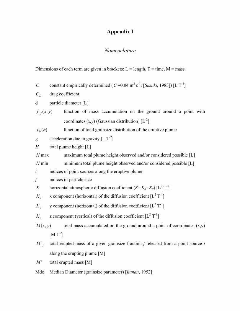
Appendix I

Nomenclature

Dimensions of each term are given in brackets: L = length, T = time, M = mass.

C constant empirically determined (C =0.04 m2 s-1; [Suzuki, 1983]) [L T-1]

DC drag coefficient

d particle diameter [L]

),(, yxf ji function of mass accumulation on the ground around a point with

coordinates (x,y) (Gaussian distribution) [L-2]

)(f function of total grainsize distribution of the eruptive plume

g acceleration due to gravity [L T-2]

H total plume height [L]

maxH maximum total plume height observed and/or considered possible [L]

minH minimum total plume height observed and/or considered possible [L]

i indices of point sources along the eruptive plume

j indices of particle size

K horizontal atmospheric diffusion coefficient (K=Kx=Ky) [L2 T-1]

xK x component (horizontal) of the diffusion coefficient [L2 T-1]

yK y component (horizontal) of the diffusion coefficient [L2 T-1]

zK z component (vertical) of the diffusion coefficient [L2 T-1]

),( yxM total mass accumulated on the ground around a point of coordinates (x,y)

[M L-2]

,oi jM total erupted mass of a given grainsize fraction j released from a point source i

along the erupting plume [M] oM total erupted mass [M]

Md Median Diameter (grainsize parameter) [Inman, 1952]

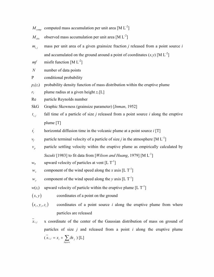
compM computed mass accumulation per unit area [M L-2]

obsM observed mass accumulation per unit area [M L-2]

,i jm mass per unit area of a given grainsize fraction j released from a point source i

and accumulated on the ground around a point of coordinates (x,y) [M L-2]

mf misfit function [M L-2]

N number of data points

P conditional probability

pz(zi) probability density function of mass distribution within the eruptive plume

ri plume radius at a given height zi [L]

Re particle Reynolds number

SkG Graphic Skewness (grainsize parameter) [Inman, 1952]

jit , fall time of a particle of size j released from a point source i along the eruptive

plume [T] 'it horizontal diffusion time in the volcanic plume at a point source i [T]

vj particle terminal velocity of a particle of size j in the atmosphere [M L-1]

pv particle settling velocity within the eruptive plume as empirically calculated by

Suzuki [1983] to fit data from [Wilson and Huang, 1979] [M L-1]

wo upward velocity of particles at vent [L T-1]

xw component of the wind speed along the x axis [L T-1]

yw component of the wind speed along the y axis [L T-1]

w(zi) upward velocity of particle within the eruptive plume [L T-1]

,x y coordinates of a point on the ground

iii zyx ,, coordinates of a point source i along the eruptive plume from where

particles are released

jix , x coordinate of the center of the Gaussian distribution of mass on ground of

particles of size j and released from a point i along the eruptive plume

(layers

jiji xxx , ) [L]

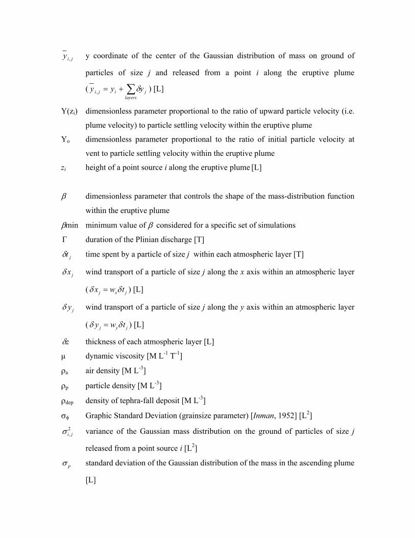
jiy , y coordinate of the center of the Gaussian distribution of mass on ground of

particles of size j and released from a point i along the eruptive plume

(layers

jiji yyy , ) [L]

Y(zi) dimensionless parameter proportional to the ratio of upward particle velocity (i.e.

plume velocity) to particle settling velocity within the eruptive plume

Yo dimensionless parameter proportional to the ratio of initial particle velocity at

vent to particle settling velocity within the eruptive plume

zi height of a point source i along the eruptive plume [L]

dimensionless parameter that controls the shape of the mass-distribution function

within the eruptive plume

min minimum value of considered for a specific set of simulations

duration of the Plinian discharge [T]

jt time spent by a particle of size j within each atmospheric layer [T]

jx wind transport of a particle of size j along the x axis within an atmospheric layer

( j x jx w t ) [L]

jy wind transport of a particle of size j along the y axis within an atmospheric layer

( j y jy w t ) [L]

z thickness of each atmospheric layer [L]

µ dynamic viscosity [M L-1 T-1]

a air density [M L-3]

p particle density [M L-3]

dep density of tephra-fall deposit [M L-3]

Graphic Standard Deviation (grainsize parameter) [Inman, 1952] [L2]2,i j variance of the Gaussian mass distribution on the ground of particles of size j

released from a point source i [L2]

p standard deviation of the Gaussian distribution of the mass in the ascending plume

[L]

granulometric unit: = -log2(103d), where d is the particle diameter in m

max maximum particle diameter

min minimum particle diameter

Figure captions

Fig. 1. Map of the North Island of New Zealand showing: (a) main cities (black

diamonds), important populated towns (grey circles: Mk, Maketu; Mt, Matata; Ec, Edgecumbe; W, Whakatane; TT, Te Teko; K, Kawerau), Tarawera Volcanic Complex (small grey triangle) and the Taupo Volcanic Zone (large shaded triangle); (b) Tarawera Volcanic Complex (adapted from Nairn [1989] and Sahetapy-Engel [2002]) with the main domes, old lava deposits and the AD 1886 eruptive fissure. The names of the 4 lava domes produced during the AD 1305 Kaharoa eruption are also shown (only Crater Dome, Ruawahia Dome and Wahanga Dome produced tephra fall; [Sahetapy-Engel, 2002]).

Fig. 2. Isopach map of total tephra-fall accumulation (cm) from the AD 1305 Kaharoa eruption [Sahetapy-Engel, 2002]. Dash line indicates 5 cm isopach. The triangle indicates the Tarawera Volcanic Complex. Note the two prominent lobes to the southwest and to the northwest.

Fig. 3. Semi-log plots showing the variation, for different particle sizes, of: (a) fall time (ti,j); (b) fall time + diffusion time in the plume (ti,j + t’i); (c) variance (σi,j

2) (eq. (6) and eq. (8)). Calculations are done between 1 and 35 km (1 km step), with K= 900 m2 s-1 and fall-time threshold=3600 s. Note how the plume diffusion time (t’i) mainly affects coarse particles ((a) and (b)). Note also the step in σi,j

2 values at 5-6 km due to the shift of diffusion law for particles with diameter of 0.25 mm (2 φ) ((c); (eq. (6) and eq. (8)).

Fig. 4. Mass fraction of particles of a specific grainsize, here specified by settling velocities of 0.25, 1, and 2.5 m s-1, released as a function of height from a volcanic plume of total height 10 km, calculated using eq. (6) and (8). Initial eruption velocity at the vent, ow , is assumed to be 100 m s-1. Substantially different curves are generated for (a) 1=β and (b) 01.0=β .

Fig. 5. Frequency plots showing output results for: (a) plume heights stochastically sampled between Log(14 km) and Log(26 km) (bin = 200 m); (b) eruptive-episode duration stochastically sampled between 2 and 6 hours (bin = 0.1 hours); (c) total erupted mass determined from the combination of plume heights and eruption duration above (eq. (13)) (bin = 2.00E+10 kg).

Fig. 6. Frequency plots showing: (a) values of β stochastically sampled between 0.5 and 1 (bin = 0.01) and (b) Mdφ stochastically sampled between -0.8 and 4 φ (bin = 0.1 φ). φ = -log2(103d), where d is the particle diameter in m. (c) Cumulative plot showing the total grainsize distribution of the Waimihia Plinian (white), Hatepe Plinian (black) and Taupo Plinian (gray) from Walker [1980] and Walker [1981]. Given that all original grainsize distributions are truncated at 3 φ, the grainsize trend beyond 3 φ is extrapolated based on a log-normal distribution. Resulting Mdφ are: -0.8, 0.6 and 4 φ respectively. Resulting σφ are: 2.3, 2.3 and 2.9 respectively.

Fig. 7. Semi-log plots showing the misfit function (mf; eq. (15)) for all points (grey diamonds; primary axis; Runs 1 in Table 1) and for distal points (white triangles; secondary axis; Runs 2 in Table 1) (17 June 1996 eruption of Ruapehu, New Zealand) calculated for: (a) diffusion coefficient, K, (b) fall-time cut off and (c) mass-

distribution parameter, β. Observed data from BF Houghton (manuscript in preparation, 2003).

Fig. 8. Log plots showing best fit for: (a) Ruapehu total data (114 data) (DC = 200 m2 s-

1; fall-time threshold = 72 s, i.e. 0.02 hours); (b) Ruapehu distal data (88 points) (DC = 600 m2 s-1; fall-time threshold = 1080 s, i.e. 0.3 hours); (c) Kaharoa F using Ruapehu distal-data best fit (DC = 600 m2 s-1; fall-time threshold=1080 s). Ruapehu proximal data (< 5 km) plotted with distal-data best fit are also shown in (b). Runs 1-3 in Table 1. The equiline is also shown for comparison. Observed data for the Ruapehu and Kaharoa eruptions are from BF Houghton (manuscript in preparation, 2003) and Sahetapy-Engel [2002] respectively.

Fig. 9. Comparison between isomass maps for the AD 1305 Kaharoa eruption (Unit F) compiled from field data (from Sahetapy-Engel [2002]) and the computed deposit. The computed deposit is run with DC = 600 m2 s-1 and fall-time cut off = 1080 s (see alsoTable 1). Tephra-fall accumulation is in kg m-2. Contours for the field-based map are spaced every 50 kg m-2; the 10 kg m-2 contour is also shown. Black dots on the field-based map indicate field data. Contours for the computed map are spaced every 10 kg m-2 up to 50 kg m-2, and every 100 kg m-2 after 100 kg m-2. Some key cities (diamonds) and Tarawera Volcano (triangle) are also shown.

Fig. 10. Density parameterization for the AD 1305 Kaharoa eruption (from Bonadonna and Phillips [2003]). Density of pumices (gray circles; 1000 kg m-3) and lithics (black triangles; 2350 kg m-3) with diameter >2 mm is directly measured [Sahetapy-Engel, 2002]. Density of lithics is assumed to be constant, whereas density of pumices with diameter <2 mm is assumed to decrease linearly and to reach the lithic density value when the fragment diameter decreases below 8 µm.

Fig. 11. Plots showing (a) mean wind direction (provenance + 180°) and (b) mean wind velocity averaged for each level (i.e. every 1 km) over 3 years of wind profiles (1996-1998) sampled 4 times a day (see text for details). The standard deviation determined for each level is also shown. NCEP Reanalysis data provided by the NOAA-CIRES Climate Diagnostics Center.

Fig. 12. Plots showing: (a) the percentage of wind profiles characterized by ≥ 15 levels with wind blowing between 0° and 90°, 90° and 180°, 180° and 270° and 270° and 360° respectively (degrees are from the North); (b) the percentage of such wind profiles distributed amongst each month. Percentages are calculated out of the total wind sample analyzed (i.e. 1996-1998).

Fig. 13. Hazard curves computed for the Upper Limit Scenario (thick line) and the Eruption Range Scenario (thin line) for key cities and towns (in Fig. 1): (a) Maketu, (b) Kawerau, (c) Tauranga, (d) Taupo, (e) Wellington and (f) Rotorua. Hazard Curves show the probability of exceeding a given accumulation of tephra fall (kg m-2). Runs 4 and 5 in Table 1.

Fig. 14. Upper Limit Scenario maps computed for a deposit threshold of: (a) 30 kg m-2 (damage to agriculture) and (b) 300 kg m-2 (minimum loading for roof collapse). The map for a 600 kg m-2 threshold is not shown as it only indicates probability <5% for the populated areas around the volcano. Contours are spaced every 10% probability of reaching a given threshold. The 5% contour is also shown (thick solid line). Key cities and towns are also shown (circles; from Fig. 1). Tarawera Volcanic Complex is indicated with a triangle. Runs 6 in Table 1.

Fig. 15. Eruption Range Scenario maps computed for a deposit threshold of 30 kg m-2 (damage to agriculture). The map for a 300 kg m-2 threshold is not shown as it only indicates probability <5% for the populated areas around the volcano. Contours are spaced every 10% probability of reaching a given threshold. The 5% contour is also shown (thick solid line). Key cities and towns are also shown (circles; from Fig. 1). Tarawera Volcanic Complex is indicated with a triangle. Runs 7 in Table 1.

Fig. 16. Multiple Eruption Scenario maps computed for a deposit threshold of: (a) 30 kg m-2 (damage to agriculture) and (b) 300 kg m-2 (minimum loading for roof collapse). The map for a 600 kg m-2 threshold is not shown as it only indicates probability <5% for most of the populated areas around the volcano (apart from Kawerau, i.e. 5%). Contours are spaced every 10% probability of reaching a given threshold. The 5% contour is also shown (thick solid line). Key cities and towns are also shown (circles; from Fig. 1). Tarawera Volcanic Complex is indicated with a triangle. Runs 8 in Table 1.

Fig. 17. Upper Limit Scenario maps computed sampling wind data (a) from June through August (austral winter; winds mainly blowing between 0° and 180°, see Fig. 7b) and (b) from September to March (austral spring-summer; when winds also blow between 180° and 360°, see Fig. 7b). Deposit threshold is 30 kg m-2 (damage to agriculture). Contours are spaced every 10% probability of reaching a given threshold. The 5% contour is also shown (thick solid line). Key cities and towns are also shown (circles; from Fig. 1). Tarawera Volcanic Complex is indicated with a triangle. Runs 9 and 10 in Table 1.

Fig. 18. Upper Limit Scenario maps computed sampling wind data (a) from 1996 (neutral conditions), (b) from 1997 through 1998 (characterized by El Niño Southern Oscillation phenomenon), (c) from April 1997 through May 1998 (characterized by a strong El Niño fluctuation) and (d) between May and December 1998 (characterized by La Niña fluctuation). Deposit threshold is 30 kg m-2 (damage to agriculture). Contours are spaced every 10% probability of reaching a given threshold. The 5% contour is also shown (thick solid line). Key cities and towns are also shown (circles; from Fig. 1). Tarawera Volcanic Complex is indicated with a triangle. Runs 11-14 in Table 1.

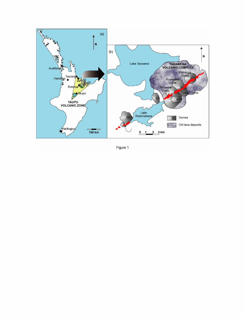
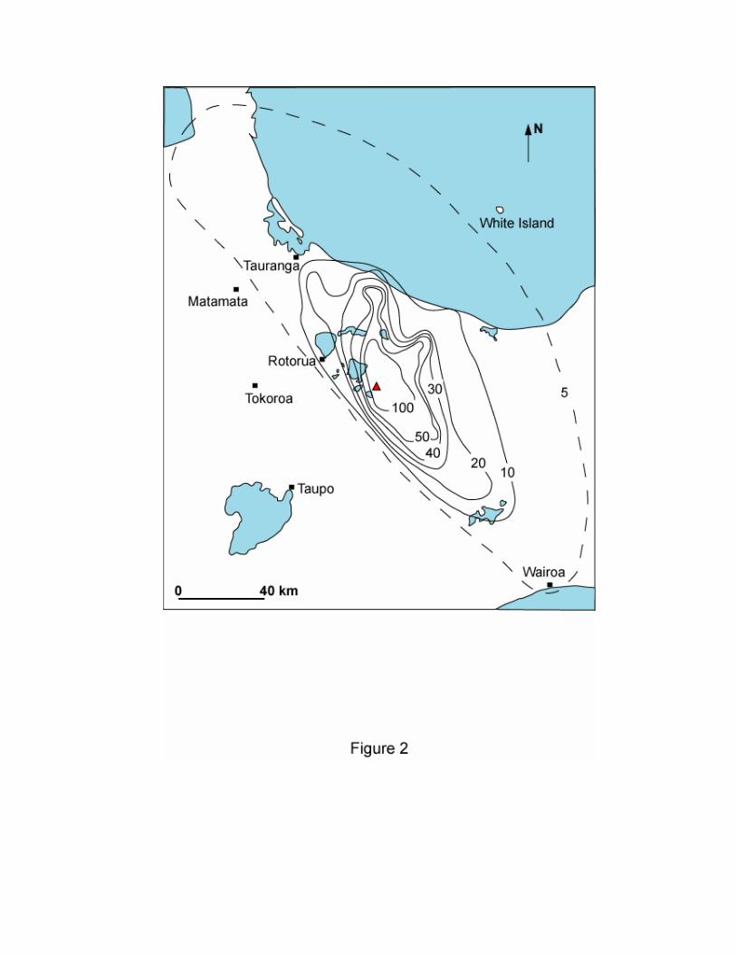
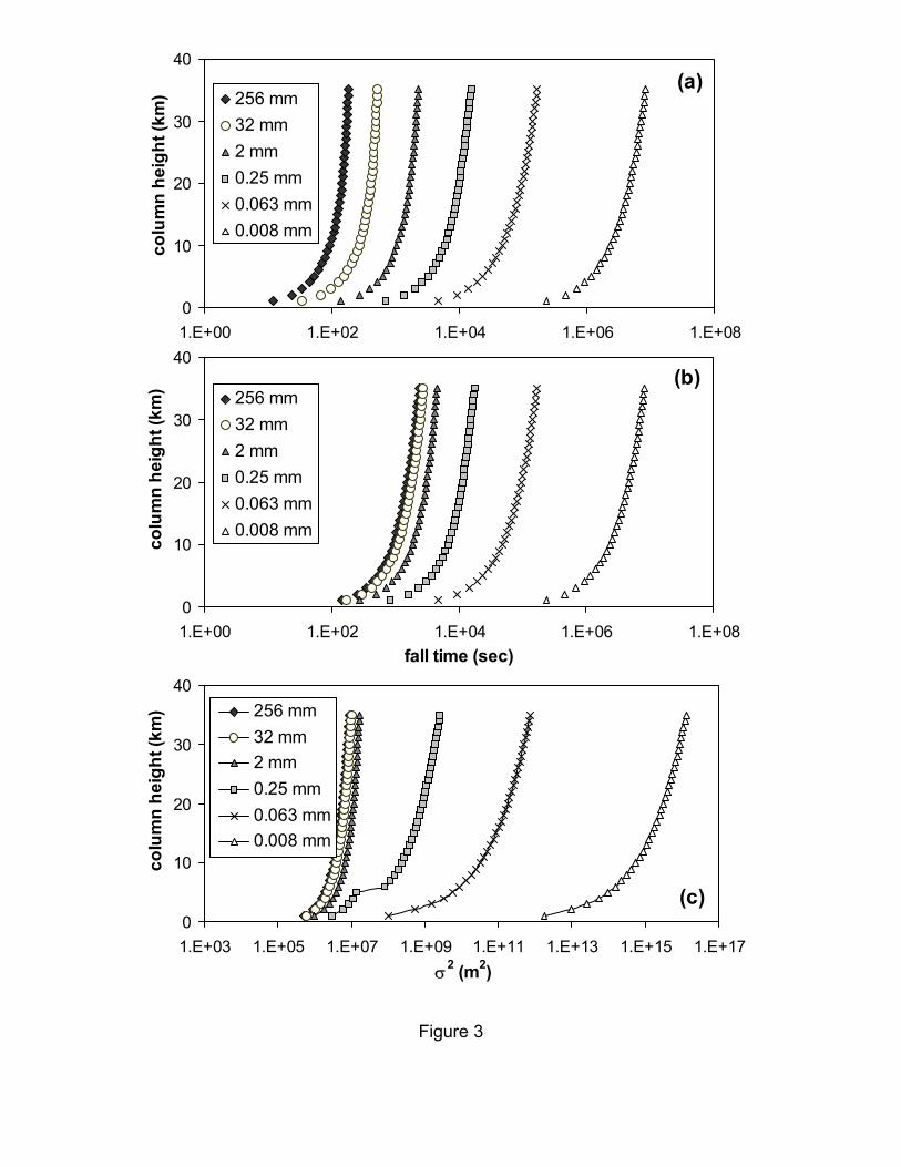
Figure 3

0

10

20

30

40

1.E+00 1.E+02 1.E+04 1.E+06 1.E+08

colu

mn

heig

ht (k

m) 256 mm

32 mm2 mm0.25 mm0.063 mm0.008 mm

(a)

0

10

20

30

40

1.E+03 1.E+05 1.E+07 1.E+09 1.E+11 1.E+13 1.E+15 1.E+17σ2 (m2)

colu

mn

heig

ht (k

m) 256 mm

32 mm2 mm0.25 mm0.063 mm0.008 mm

(c)

0

10

20

30

40

1.E+00 1.E+02 1.E+04 1.E+06 1.E+08fall time (sec)

colu

mn

heig

ht (k

m) 256 mm

32 mm2 mm0.25 mm0.063 mm0.008 mm

(b)

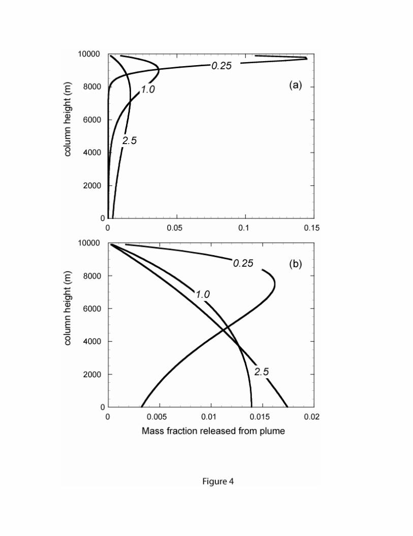
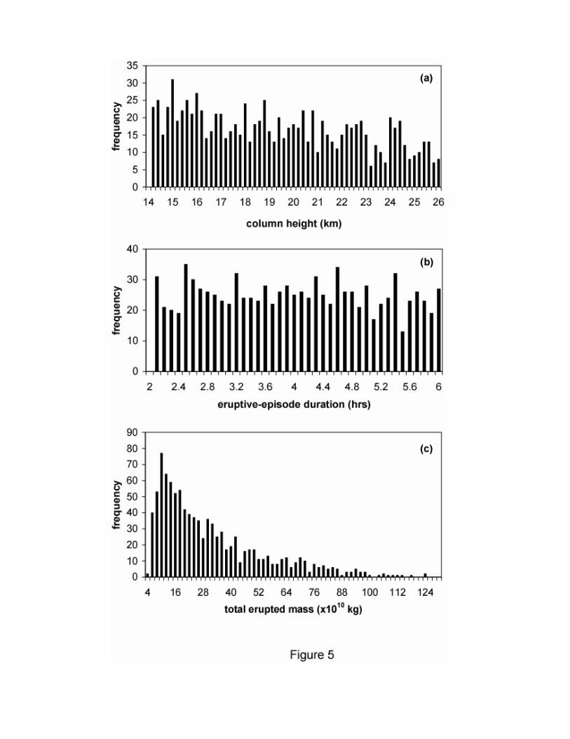
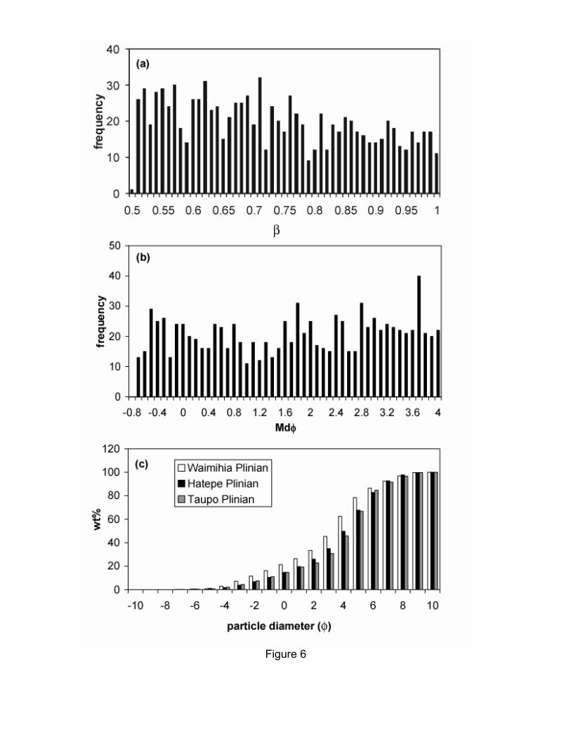
Figure 6

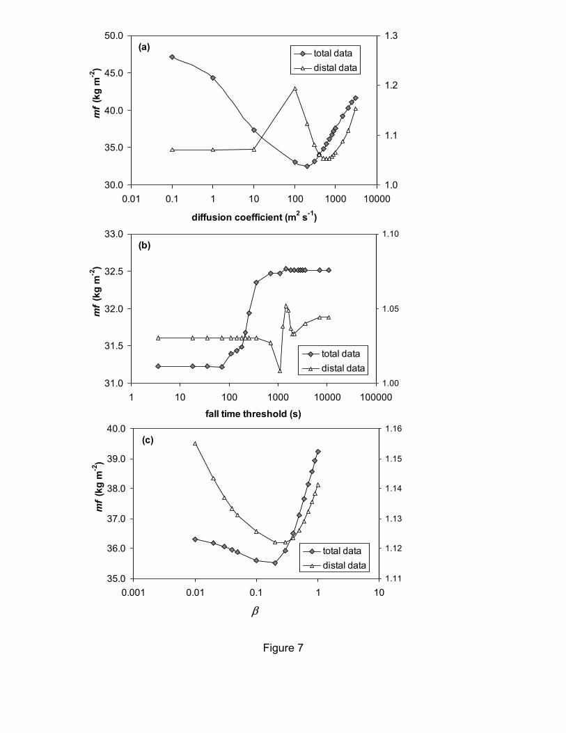
30.0

35.0

40.0

45.0

50.0

0.01 0.1 1 10 100 1000 10000

diffusion coefficient (m2 s-1)

mf

(kg

m-2

)

1.0

1.1

1.2

1.3

total datadistal data

(a)

31.0

31.5

32.0

32.5

33.0

1 10 100 1000 10000 100000

fall time threshold (s)

mf

(kg

m-2

)

1.00

1.05

1.10

total datadistal data

(b)

35.0

36.0

37.0

38.0

39.0

40.0

0.001 0.01 0.1 1 10

β

mf

(kg

m-2

)

1.11

1.12

1.13

1.14

1.15

1.16

total datadistal data

(c)

Figure 7

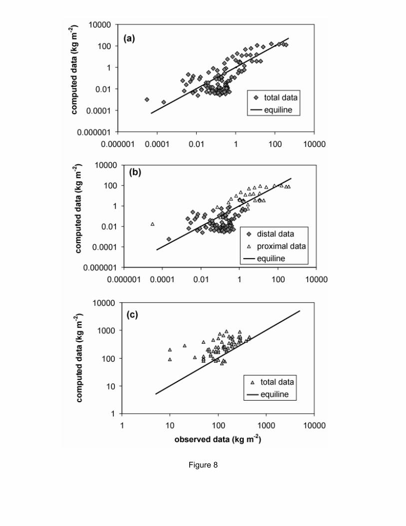
Figure 8

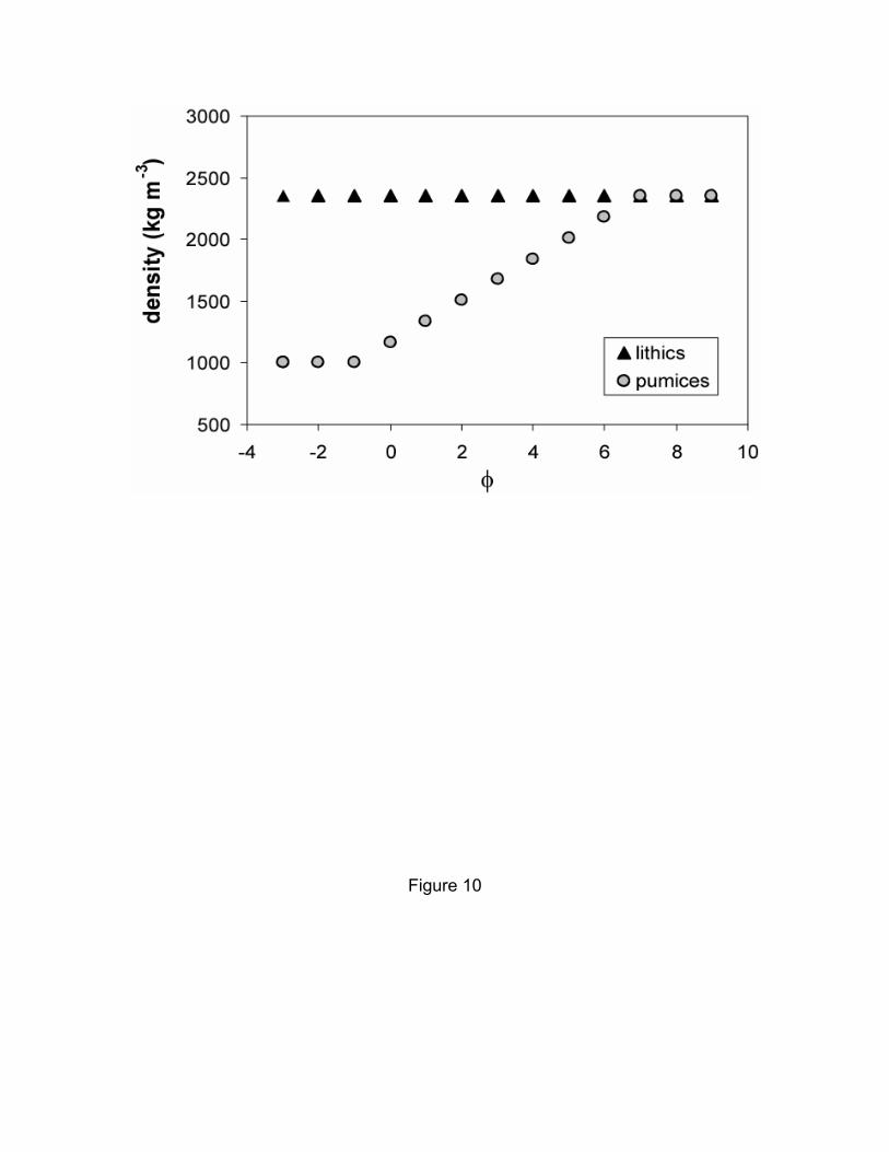
Figure 10

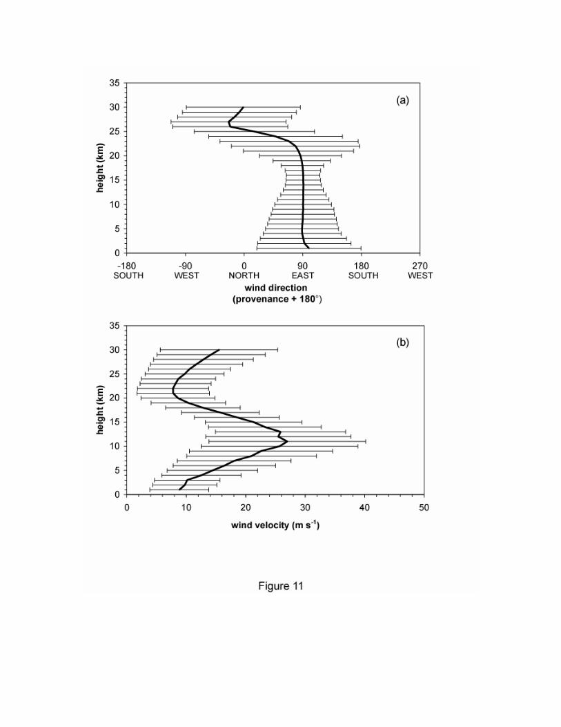
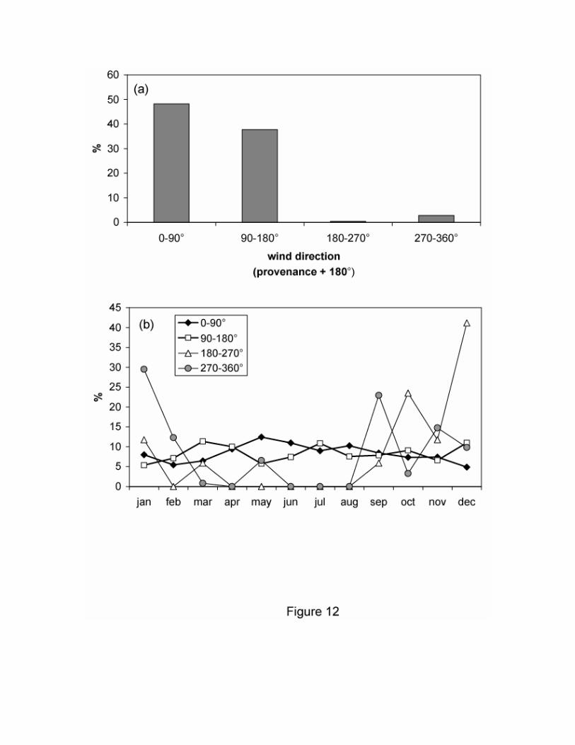
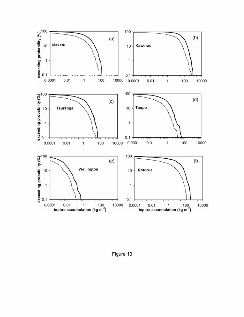
Figure 13