Problem Gambling and Crime

Earl L. Grinols,∗ David B. Mustard,†

DRAFT

NOT FOR QUOTATION:

22 March 2016

Abstract

We evaluate the connection between problem gambling and the incidence of crime outcomesusing five years of survey panel data collected on 4,123 subjects for the Ontario Problem GamblingResearch Centre. Problem gambling is statistically significantly associated with elevated rates ofcrime. This connection persists even after controlling for an extensive set of demographic and ed-ucation characteristics and measures of alcohol and drug use and mental health. We estimate thatbeing a problem gambler increases ones likelihood of committing crime by 4.28 to 7.63 percentagepoints even when the nearest casino is more than 105 kilometers (over 64 miles) away.

Key Words: Problem gambling, social costs, causality.

JEL Classification Numbers: L8, O2, R5.

∗Department of Economics, Hankamer School of Business, Baylor University, One Bear Place #98003, Waco, Texas76798; Tel. (254) 710-1903.

†Department of Economics, Terry College of Business, University of Georgia and the Institute for the Study of Labor.

1 Introduction

Does casino gambling increase crime? Grinols and Mustard (2006) document that counties that open

casinos have crime rates about 8 percentage points higher than their counterparts that do not open a

casino. They identify many reasons why casinos could increase or decrease crime and estimate a total

effect, which they cannot disaggregate into specific factors. However, their finding that crime rates in

casino counties remain relatively stable for two or three years after casinos open and then increase over

time suggests that problem gamblers, who may take a few years to develop into problem gamblers and

to exhaust their resources before committing crime, may play an important role.

Although studies suggest links between problem gambling and crime (Grinols and Mustard, 2006,

provide a review), there is little hard evidence because of three substantial unresolved issues. First,

research frequently relies upon small and non-representative samples. Second, no study systematically

investigates individual data of gambling behavior and criminal participation. Third, studies lack a

comprehensive set of controls that allow researchers to net out other addictive characteristics when

estimating the effect of problem gambling. This last problem is particularly nettlesome because there is

a strong correlation between pathological gambling and other addictive behavior, such as alcohol and

substance abuse.1 “A relevant question to ask,” warns the National Research Council, “is whether,

in the absence of legalized gambling, a pathological gambler would have engaged in some similarly

destructive and costly addiction, such as alcoholism. To the extent that the answer is yes, the costs...

represent transfer of costs from one problem category to another.”2 We present quantitative research

in this paper that responds to all three concerns.

The chain of causal connection appears to be that by expanding the number of gambling locations the

cost of gambling to the user is lowered and its quantity increased. Greater access combined with latent

susceptibility to problem gambling in the general population creates problem gamblers who engage in

1National Research Council, 1999, p. 170.2Ibid., p. 171.

1

socially costly outcomes like crime. We therefore examine the relationship between problem gamblers and

crime. Our data set consists of 4,123 people from Ontario, Canada who are interviewed each year over a

five-year period. This Quinte Exhibition Raceway (QER) Survey has a remarkable retention rate of 94%

and reports criminal activity plus an array of gambling behaviors that determine whether respondents are

problem gamblers. In addition, the data set has extensive variables on personal characteristics, mental

health, and alcohol and drug use that are correlated with gambling behavior but often omitted from

other data sets. With these data, we can address the three problems that plague other studies.

The rest of this paper is organized as follows. Section 2 contrasts average differences between

problem gamblers and people without gambling problems. Section 3 uses model-free nonparametric

statistics to compare problem gamblers to those who do not have gambling problems. The evidence

rejects the null hypothesis that the two samples come from the same distribution. We then test whether

people who are problem gamblers and also exhibit alcohol abuse, drug abuse, or mental health issues or

those who exhibit none of the above are equally likely to commit crime. Again, the data reject the null

hypothesis that the two groups are drawn from the same distribution and indicate that the dominant

causal factor in crime is problem gambling. Section 4 uses parametric regressions to model the interaction

of problem gambling, substance abuse, and mental health. We also correct for possible endogeneity

of problem gambling using propensity score matching methods and instrumental variable techniques.

Section 5 provides a series of robustness and reliability checks that involve different measures of problem

gambling, substance abuse and mental health. Section 6 uses our estimates to make inferences about

the magnitude of the crime effects. Section 7 summarizes and concludes. We estimate that being a

problem gambler increases ones likelihood of committing crime by 5.1 to 6.0 percent even when the

nearest casino is more than 105 kilometers (over 64 miles) away.

2

2 Data

We use data from the five-year Quinte Exhibition Raceway (QER) survey of individuals from Quinte in

southern Ontario, Canada, which is located just north of Lake Ontario. The Ontario Problem Gambling

Research Centre did the survey, which was funded by a five-year $3.1 million grant.3 The panel sur-

vey included 4,123 participants each year for five years, yielding 20,615 potential observations. 3,000

participants were randomly selected. Because one of the main goals of the initiative was to examine

problem gamblers, which most studies conclude constitute less than 5 percent of the population (Gupta,

1997; Potenza, 2008), the remaining 1,123 participants were oversampled with respect to being problem

gamblers. Attrition reduced the final sample to 19,583 observations, or an impressive 94% retention

rate. For our empirical work, we excluded five additional observations that lacked complete informa-

tion on some mental health variables. The final sample that we use for the empirical work has 19,578

observations.

The QER survey was originally undertaken with the expectation that a casino with electronic gaming

machines would open in Quinte mid-survey, providing a natural experiment to compare baseline gam-

bling behavior with gambling behavior after the casino was opened. However, a Quinte casino never

opened. Although the original intent was not realized, the data became an ideal panel of observations

on individuals who live between 75 and 105 km from the closest gambling facility.

The study provided respondents with strict guarantees of confidentiality.4 Activities reported ranged

3“Examining the Impact of a Race Track Slots Facility in the Belleville, Ontario Area.” February 24, 2006 Research

Proposal submitted to the Ontario Problem Gambling Research Centre. Robert Williams and Robert Hann, principal

investigators; co-investigators Donald Schopflocher, Robert Wood; consultants Earl L. Grinols, Jan McMillen. Term of

project April 1, 2006–February 28, 2012.4The grant document reports, “The strict confidentiality of the information provided will be emphasized. Participants’

data will be automatically converted to an SPSS file with only the Principal Investigators having access to that file.

Participants will also be asked to identify 2 friends/relatives who would be in the best position to verify information

the participant provided, as among the 4,000 participants a small percentage of randomly selected collaterals may be

contacted to corroborate this information. Although it is unlikely that we will actually contact collaterals, the possibility

of independent corroboration significantly improves validity of self-report (Babor et al., 1987; Roese and Jamieson, 1993;

3

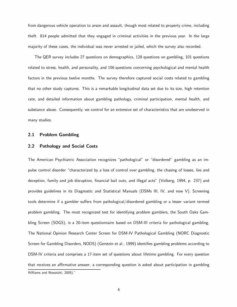
from dangerous vehicle operation to arson and assault, though most related to property crime, including

theft. 814 people admitted that they engaged in criminal activities in the previous year. In the large

majority of these cases, the individual was never arrested or jailed, which the survey also recorded.

The QER survey includes 27 questions on demographics, 128 questions on gambling, 101 questions

related to stress, health, and personality, and 156 questions concerning psychological and mental health

factors in the previous twelve months. The survey therefore captured social costs related to gambling

that no other study captures. This is a remarkable longitudinal data set due to its size, high retention

rate, and detailed information about gambling pathology, criminal participation, mental health, and

substance abuse. Consequently, we control for an extensive set of characteristics that are unobserved in

many studies.

2.1 Problem Gambling

2.2 Pathology and Social Costs

The American Psychiatric Association recognizes “pathological” or “disordered” gambling as an im-

pulse control disorder “characterized by a loss of control over gambling, the chasing of losses, lies and

deception, family and job disruption, financial bail outs, and illegal acts” (Volberg, 1994, p. 237) and

provides guidelines in its Diagnostic and Statistical Manuals (DSMs III, IV, and now V). Screening

tools determine if a gambler suffers from pathological/disordered gambling or a lesser variant termed

problem gambling. The most recognized test for identifying problem gamblers, the South Oaks Gam-

bling Screen (SOGS), is a 20-item questionnaire based on DSM-III criteria for pathological gambling.

The National Opinion Research Center Screen for DSM-IV Pathological Gambling (NORC Diagnostic

Screen for Gambling Disorders, NODS) (Gerstein et al., 1999) identifies gambling problems according to

DSM-IV criteria and comprises a 17-item set of questions about lifetime gambling. For every question

that receives an affirmative answer, a corresponding question is asked about participation in gambling

Williams and Nowatzki, 2005).”

4

over the last year.

For this survey, questions sufficient to construct both the SOGS and NODS as well as the Canadian

Problem Gambling Index (CPGI) and the Problem and Pathological Gambling Measure (PPGM) were

administered. All the questions from the NODS screen and most questions required for the SOGS screen

were included directly. For the SOGS questions that were not directly asked, very similar equivalent

questions were asked that generate a synthetic SOGS score.

For robustness reasons, we use both SOGS and NODS to identify people who have problems with

gambling. This paper uses the term “problem” gambler to include both the “problem” and “pathologi-

cal” gambler categories that are identified by SOGS and NODS. Our conclusions do not depend on the

particular screen selected.

Table 1 reports the descriptive statistics for the first year in the sample by non-problem and problem

gamblers as identified by the SOGS. Of the 4,120 individuals who were surveyed, 10.4 percent were

problem gamblers and 89.2 percent were not. Problem gamblers engage in Class III gambling more

heavily than the non-problem group. Their annual median losses ($1560) are more than eight times

those who are not problem gamblers ($192) and their average annual losses are $5434 compared to

$778. Similarly, problem gamblers gambled 177 days in the previous year compared to an average of 68

dates for non-problem gamblers.

Table 1 also displays the share of gamblers who admitted to committing a crime in the past year.

Problem gamblers are 297 percent more likely to have committed a crime in the previous year than

non-problem gamblers (10.1 percent compared to 3.4 percent).

One enormous advantage of our data set is that we have detailed information on many health and

social factors, such as substance abuse and mental health. Problem gamblers frequently have “multiple

overlapping personality disorders” (Blaszczynski and Steel 1998, p. 60). Welte et al. (2004) conclude

that substance abuse is a good predictor of problem gambling. Shaffer and Korn (2002) find that 25-63

percent of pathological gamblers satisfy criteria for lifetime substance abuse. Mental health is also a

5

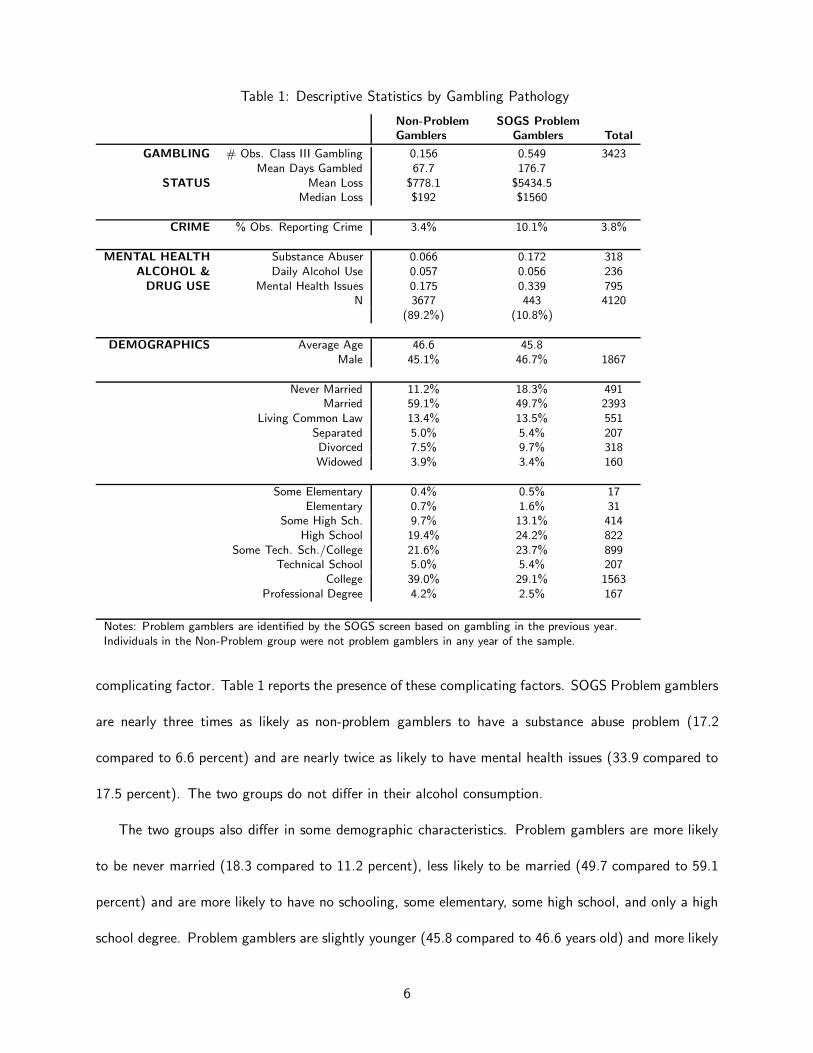
Table 1: Descriptive Statistics by Gambling Pathology

Non-Problem SOGS Problem

Gamblers Gamblers Total

GAMBLING # Obs. Class III Gambling 0.156 0.549 3423Mean Days Gambled 67.7 176.7

STATUS Mean Loss $778.1 $5434.5Median Loss $192 $1560

CRIME % Obs. Reporting Crime 3.4% 10.1% 3.8%

MENTAL HEALTH Substance Abuser 0.066 0.172 318ALCOHOL & Daily Alcohol Use 0.057 0.056 236

DRUG USE Mental Health Issues 0.175 0.339 795N 3677 443 4120

(89.2%) (10.8%)

DEMOGRAPHICS Average Age 46.6 45.8Male 45.1% 46.7% 1867

Never Married 11.2% 18.3% 491Married 59.1% 49.7% 2393

Living Common Law 13.4% 13.5% 551Separated 5.0% 5.4% 207Divorced 7.5% 9.7% 318Widowed 3.9% 3.4% 160

Some Elementary 0.4% 0.5% 17Elementary 0.7% 1.6% 31

Some High Sch. 9.7% 13.1% 414High School 19.4% 24.2% 822

Some Tech. Sch./College 21.6% 23.7% 899Technical School 5.0% 5.4% 207

College 39.0% 29.1% 1563Professional Degree 4.2% 2.5% 167

Notes: Problem gamblers are identified by the SOGS screen based on gambling in the previous year.Individuals in the Non-Problem group were not problem gamblers in any year of the sample.

complicating factor. Table 1 reports the presence of these complicating factors. SOGS Problem gamblers

are nearly three times as likely as non-problem gamblers to have a substance abuse problem (17.2

compared to 6.6 percent) and are nearly twice as likely to have mental health issues (33.9 compared to

17.5 percent). The two groups do not differ in their alcohol consumption.

The two groups also differ in some demographic characteristics. Problem gamblers are more likely

to be never married (18.3 compared to 11.2 percent), less likely to be married (49.7 compared to 59.1

percent) and are more likely to have no schooling, some elementary, some high school, and only a high

school degree. Problem gamblers are slightly younger (45.8 compared to 46.6 years old) and more likely

6

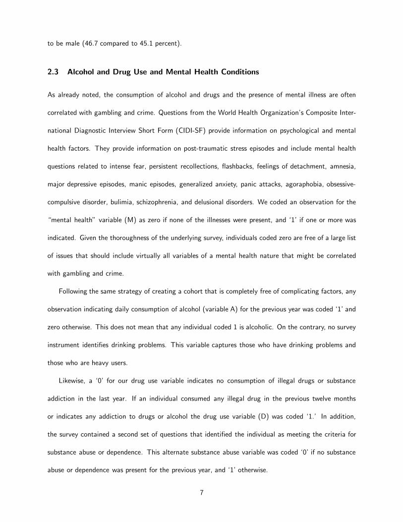
to be male (46.7 compared to 45.1 percent).

2.3 Alcohol and Drug Use and Mental Health Conditions

As already noted, the consumption of alcohol and drugs and the presence of mental illness are often

correlated with gambling and crime. Questions from the World Health Organization’s Composite Inter-

national Diagnostic Interview Short Form (CIDI-SF) provide information on psychological and mental

health factors. They provide information on post-traumatic stress episodes and include mental health

questions related to intense fear, persistent recollections, flashbacks, feelings of detachment, amnesia,

major depressive episodes, manic episodes, generalized anxiety, panic attacks, agoraphobia, obsessive-

compulsive disorder, bulimia, schizophrenia, and delusional disorders. We coded an observation for the

“mental health” variable (M) as zero if none of the illnesses were present, and ‘1’ if one or more was

indicated. Given the thoroughness of the underlying survey, individuals coded zero are free of a large list

of issues that should include virtually all variables of a mental health nature that might be correlated

with gambling and crime.

Following the same strategy of creating a cohort that is completely free of complicating factors, any

observation indicating daily consumption of alcohol (variable A) for the previous year was coded ‘1’ and

zero otherwise. This does not mean that any individual coded 1 is alcoholic. On the contrary, no survey

instrument identifies drinking problems. This variable captures those who have drinking problems and

those who are heavy users.

Likewise, a ‘0’ for our drug use variable indicates no consumption of illegal drugs or substance

addiction in the last year. If an individual consumed any illegal drug in the previous twelve months

or indicates any addiction to drugs or alcohol the drug use variable (D) was coded ‘1.’ In addition,

the survey contained a second set of questions that identified the individual as meeting the criteria for

substance abuse or dependence. This alternate substance abuse variable was coded ‘0’ if no substance

abuse or dependence was present for the previous year, and ‘1’ otherwise.

7

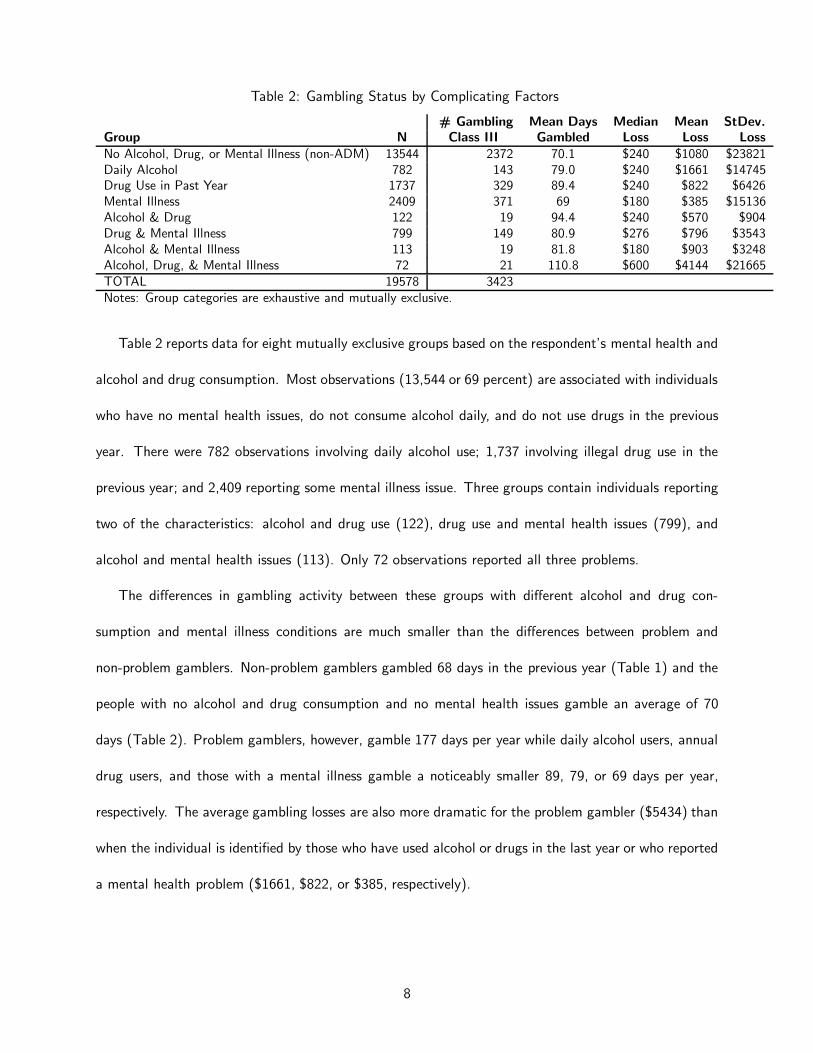
Table 2: Gambling Status by Complicating Factors

# Gambling Mean Days Median Mean StDev.

Group N Class III Gambled Loss Loss Loss

No Alcohol, Drug, or Mental Illness (non-ADM) 13544 2372 70.1 $240 $1080 $23821Daily Alcohol 782 143 79.0 $240 $1661 $14745Drug Use in Past Year 1737 329 89.4 $240 $822 $6426Mental Illness 2409 371 69 $180 $385 $15136Alcohol & Drug 122 19 94.4 $240 $570 $904Drug & Mental Illness 799 149 80.9 $276 $796 $3543Alcohol & Mental Illness 113 19 81.8 $180 $903 $3248Alcohol, Drug, & Mental Illness 72 21 110.8 $600 $4144 $21665TOTAL 19578 3423Notes: Group categories are exhaustive and mutually exclusive.

Table 2 reports data for eight mutually exclusive groups based on the respondent’s mental health and

alcohol and drug consumption. Most observations (13,544 or 69 percent) are associated with individuals

who have no mental health issues, do not consume alcohol daily, and do not use drugs in the previous

year. There were 782 observations involving daily alcohol use; 1,737 involving illegal drug use in the

previous year; and 2,409 reporting some mental illness issue. Three groups contain individuals reporting

two of the characteristics: alcohol and drug use (122), drug use and mental health issues (799), and

alcohol and mental health issues (113). Only 72 observations reported all three problems.

The differences in gambling activity between these groups with different alcohol and drug con-

sumption and mental illness conditions are much smaller than the differences between problem and

non-problem gamblers. Non-problem gamblers gambled 68 days in the previous year (Table 1) and the

people with no alcohol and drug consumption and no mental health issues gamble an average of 70

days (Table 2). Problem gamblers, however, gamble 177 days per year while daily alcohol users, annual

drug users, and those with a mental illness gamble a noticeably smaller 89, 79, or 69 days per year,

respectively. The average gambling losses are also more dramatic for the problem gambler ($5434) than

when the individual is identified by those who have used alcohol or drugs in the last year or who reported

a mental health problem ($1661, $822, or $385, respectively).

8

3 Nonparametric Statistics

To consider whether problem gambling impacts crime we first examine the raw data and then apply

non-parametric statistical tests to them. The numbers in Table 1 are the first evidence. If an observation

applies to a non-problem gambler, there is a 3.4 percent chance that a crime was committed in the

previous year. If the observation applies to a problem gambler, the probability rises to 10.1 percent.

Problem gamblers are therefore (294%) more likely engage in crime than are those who are not problem

gamblers. Whether the observed increase rises to the level of statistical significance is the purpose of

the tests reported next.

3.1 Kruskal-Wallis and Wilcoxon-Mann-Whitney Tests

Non-parametric statistics provide information about the statistical significance of the observed differ-

ences between two or more distributions. They are particularly valuable because they do not impose

assumptions onto the populations from which the samples are drawn. If the null hypothesis that problem

gambling does not matter to crime applies, then dividing the sample with respect to that status should

not matter to the observed quantity of crime in the two sample groups.

Kruskal-Wallis statistics test whether two or more samples are drawn from the same population.

When only two groups are present, Kruskal-Wallis is identical to the bilateral Wilcoxon-Mann-Whitney

test.

Table 3 reports the results of the Kruskal-Wallis test. The test rejects the null hypothesis that

problem gamblers and non-problem gamblers are drawn from the same distribution with respect to

crime. The K-W score is 108.899 and has a P-value of 0.0001, which strongly rejects the hypothesis.5

Thus, non-parametric statistics indicate that the elevated crime rates observed for problem gamblers

5We also compared three populations: Problem gamblers who are not pathological, pathological gamblers, and non-

problem, non-pathological gamblers. The Kruskal-Wallis score is 109.695, rejecting the null hypothesis of identical distri-

bution with a P-value of 0.0001.

9

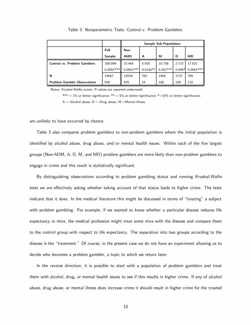
Table 3: Nonparametric Tests: Control v. Problem Gamblers

Sample Sub-Populations

Full

Sample

Non-

AMD A M D MD

Control vs. Problem Gamblers 108.899 23.464 5.935 10.758 2.722 17.021

0.0001*** 0.0001*** 0.0148** 0.001*** 0.099* 0.0001***

N 19567 13539 782 2405 1737 799

Problem Gambler Observations 930 476 24 186 100 110

Notes: Kruskal-Wallis scores. P-values are reported underneath.

*** = 1% or better significance; ** = 5% or better significance; *=10% or better significance.

A = Alcohol abuse, D = Drug abuse, M =Mental illness.

are unlikely to have occurred by chance.

Table 3 also compares problem gamblers to non-problem gamblers where the initial population is

identified by alcohol abuse, drug abuse, and/or mental health issues. Within each of the five largest

groups (Non-ADM, A, D, M, and MD) problem gamblers are more likely than non-problem gamblers to

engage in crime and this result is statistically significant.

By distinguishing observations according to problem gambling status and running Kruskal-Wallis

tests we are effectively asking whether taking account of that status leads to higher crime. The tests

indicate that it does. In the medical literature this might be discussed in terms of “treating” a subject

with problem gambling. For example, if we wanted to know whether a particular disease reduces life

expectancy in mice, the medical profession might treat some mice with the disease and compare them

to the control group with respect to life expectancy. The separation into two groups according to the

disease is the “treatment.” Of course, in the present case we do not have an experiment allowing us to

decide who becomes a problem gambler, a topic to which we return later.

In the reverse direction, it is possible to start with a population of problem gamblers and treat

them with alcohol, drug, or mental health issues to see if this results in higher crime. If any of alcohol

abuse, drug abuse, or mental illness does increase crime it should result in higher crime for the treated

10

observations. The results are that in no case does identifying observations exhibiting alcohol abuse, drug

abuse, or mental health issues in a beginning population of problem gamblers reject the null hypothesis

of no differential effect and lead to statistically significant Kruskal-Wallis scores.

The implication from non-parametric statistics is that observing problem gambling in a starting

population is associated with statistically significantly higher number of crime incidents. This is true

whether the starting population is the control group (non-A, non-D, non-M) or a group suffering from

alcohol abuse, drug abuse, or mental health issues as shown in Table 3. The reverse is not true:

individuals exhibiting problem gambling do not have discernibly higher crime outcomes when observed

to suffer in addition from alcohol, drug, or mental health issues. Thus, problem gambling appears to

be a relevant causal factor. In the next section we apply parametric statistics to model the impact of

problem gambling, alcohol, drugs, and mental health factors on crime. Because we have a large sample

that tests negatively for the presence of alcohol, drug, or mental issues we can estimate the pure effect

of problem gambling on crime. We also report the contribution of the other factors.

4 Empirical Results

Modelling allows us to estimate the increase in crime due to problem gambling and the increase due to

other factors.

4.1 Problem Gambling

Table 4 summarizes the results of probit regressions that predict the probability of crime conditional on

demographic factors and the presence or absence of problem gambling. The demographic variables used

are the same list of age and sex variables reported in Table 1.

Consider first column (2) of Table 4. This regression restricts the sample to observations with no

drug, no alcohol, and no mental health issues present. Problem gambling has a positive and statistically

significant impact on crime. The coefficient is significant at better than the one percent level.

11

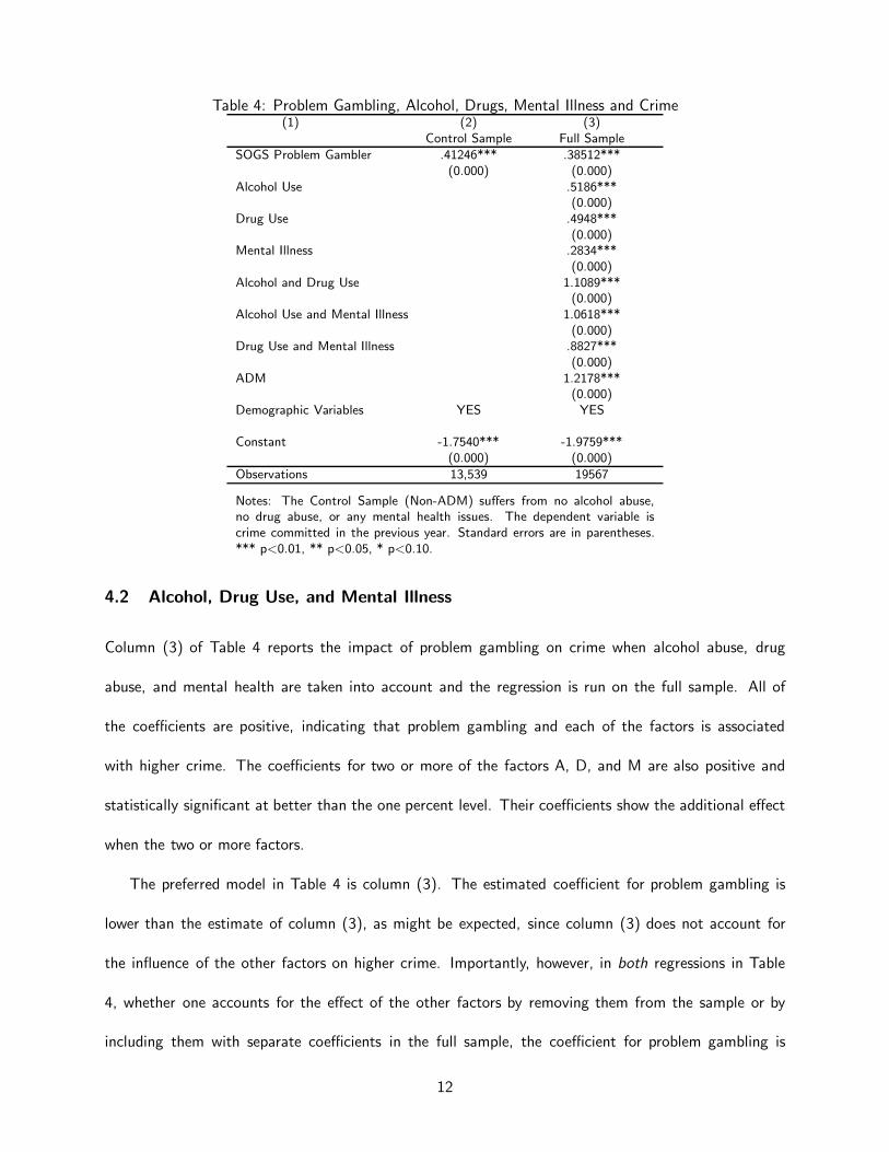
Table 4: Problem Gambling, Alcohol, Drugs, Mental Illness and Crime(1) (2) (3)

Control Sample Full Sample

SOGS Problem Gambler .41246*** .38512***(0.000) (0.000)

Alcohol Use .5186***(0.000)

Drug Use .4948***(0.000)

Mental Illness .2834***(0.000)

Alcohol and Drug Use 1.1089***(0.000)

Alcohol Use and Mental Illness 1.0618***(0.000)

Drug Use and Mental Illness .8827***(0.000)

ADM 1.2178***(0.000)

Demographic Variables YES YES

Constant -1.7540*** -1.9759***(0.000) (0.000)

Observations 13,539 19567

Notes: The Control Sample (Non-ADM) suffers from no alcohol abuse,no drug abuse, or any mental health issues. The dependent variable iscrime committed in the previous year. Standard errors are in parentheses.*** p<0.01, ** p<0.05, * p<0.10.

4.2 Alcohol, Drug Use, and Mental Illness

Column (3) of Table 4 reports the impact of problem gambling on crime when alcohol abuse, drug

abuse, and mental health are taken into account and the regression is run on the full sample. All of

the coefficients are positive, indicating that problem gambling and each of the factors is associated

with higher crime. The coefficients for two or more of the factors A, D, and M are also positive and

statistically significant at better than the one percent level. Their coefficients show the additional effect

when the two or more factors.

The preferred model in Table 4 is column (3). The estimated coefficient for problem gambling is

lower than the estimate of column (3), as might be expected, since column (3) does not account for

the influence of the other factors on higher crime. Importantly, however, in both regressions in Table

4, whether one accounts for the effect of the other factors by removing them from the sample or by

including them with separate coefficients in the full sample, the coefficient for problem gambling is

12

positive and statistically significant at better than the one percent level.

In summary, probit modelling indicates that those who are designated as problem gamblers by SOGS

are more likely to commit crime than those who are not problem gamblers. This is true for individuals

who have no known related addictions or problems, and it is true for individuals who suffer from one

or more problems related to alcohol abuse, drug abuse, and mental health. Alcohol abuse, drug abuse,

and mental health problems are themselves all associated with higher crime rates in the data, but when

accounted for do not negate the causal connection between problem gambling and crime.

4.3 Endogeneity

The way in which problem gambling can cause crime is natural and easy to explain. Individuals who

previously engaged in no crime gamble away family savings and assets and turn to crime such as theft,

fraud, and embezzlement for money. The Sheboygan, Wisconsin 64-year old grandmother and mother

of seven who embezzled money from her employer, the Kettle Moraine Employees Credit Union, over

a 10-year period and driving it out of business is an example of this type.6 The former mayor of San

Diego who was convicted of felony theft of over $2 million from a charitable foundation in consequence

of problem gambling is another. Another individual, Marilyn Lancelot, who embezzled and served prison

time said, “There wasn’t anything I wouldn’t do to get more money to gamble.”7 In addition, individuals

who previously engaged in crime may increase their crime in response to problem gambling.

The reverse direction is more problematic. That is, we do not believe that crime causes problem

gambling. But to allow for this possibility we applied propensity score matching and treatment effect

methodology to correct for endogeneity. Separately, we also used instrumental variable techniques. In

each case, the positive connection between problem gambling and crime remains.

6Milwaukee Journal Sentinel, 9 August 20007Jaret and Hogan, 2014, pp. 24-28. Grinols and Mustard, 2006, p.32 provide other examples.

13

4.3.1 Treatment Effects

Random sampling is designed to deal with the possibility that problem gambling does not have an

independent impact on crime, but the case might be present that underlying unobservables that cause

problem gambling also cause crime. Replicating the effects of a random experiment is the domain of

the treatment effects literature. Propensity score-matching for causal studies is described by Dehejia

and Wahba (2002).

In the case of rats, two groups cannot literally be identical in all respects, but can be comparable in

relevant characteristics. In the absence of treatment, two groups should have the same health outcomes.

If a drug is injected into one group and found to lead to no measurable health differences between the

two populations, it has no causal health impact.

Score-matching tries to replicate the effects of random sampling. Members of the control group are

matched with comparable subjects that have the same propensity to be a problem gambler, but differ

only with respect to the factor to be tested. The underlying factors that cause problem gambling and

crime are used in producing the two groups. Under the null hypothesis problem gambling is not a cause

of higher crime and therefore taking account of it in the matched sample should have no impact on

crime differences. This is a testable implication.

Score-matching uses a logit model to convert many variables that contribute to problem gambling

into a propensity score on which observations are matched. Higher values indicate a greater probability

of problem gambling. Included in the underlying variables are demographic variables and gambling-

related variables. The dependent variable takes the value 1 if the individual satisfied the criteria for

being a problem gambler and zero otherwise. Regressors are sex; age; age2; eight education variables;

five marital status variables; have children; employed fulltime; class III gambler; drivetime to the nearest

casino; distance to the nearest casino; a gambler in childhood family; parents, brothers, or sisters gamble

with you as a child; a problem gambler in childhood family; started gambling before age 19; frequency

14

of gambling before age 19; big win or loss before age 19; family member with a history of addiction;

family member with history of mental health problem. Including the constant, once the possible answers

were coded there were over 30 coefficients estimated in the matching logistic regression. A propensity

score is identified for each individual in the sample using our estimated logit model. We introduce a

new variable labeled problem gambler to indicate whether an individual is ever associated with problem

gambling during our sample period. These individuals are matched with like individuals (same problem

gambling propensity score) who did not develop problem gambling.

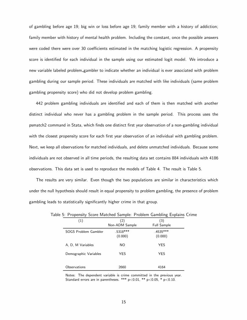
442 problem gambling individuals are identified and each of them is then matched with another

distinct individual who never has a gambling problem in the sample period. This process uses the

psmatch2 command in Stata, which finds one distinct first year observation of a non-gambling individual

with the closest propensity score for each first year observation of an individual with gambling problem.

Next, we keep all observations for matched individuals, and delete unmatched individuals. Because some

individuals are not observed in all time periods, the resulting data set contains 884 individuals with 4186

observations. This data set is used to reproduce the models of Table 4. The result is Table 5.

The results are very similar. Even though the two populations are similar in characteristics which

under the null hypothesis should result in equal propensity to problem gambling, the presence of problem

gambling leads to statistically significantly higher crime in that group.

Table 5: Propensity Score Matched Sample: Problem Gambling Explains Crime

(1) (2) (3)Non-ADM Sample Full Sample

SOGS Problem Gambler .5318*** .4535***(0.000) (0.000)

A, D, M Variables NO YES

Demographic Variables YES YES

Observations 2660 4164

Notes: The dependent variable is crime committed in the previous year.Standard errors are in parentheses. *** p<0.01, ** p<0.05, * p<0.10.

15

4.3.2 Instrumental Variable Techniques to Account for Possible Endogeneity

The South Oaks Gambling Screen incorporates questions implying a score that lies between 0 and 20.

We tested the implications of replacing the binomial variable for problem gambling (SOGS total score of

5 or higher) with the original South Oaks Gambling Screen total and running two tests with correction

for possible endogeneity. The results indicate that higher SOGS scores are associated with statistically

significantly increased levels of crime, even after instrumental variable techniques are used.

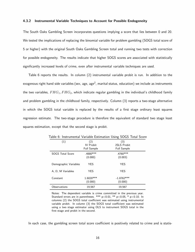
Table 6 reports the results. In column (2) instrumental variable probit is run. In addition to the

exogenous right hand side variables (sex, age, age2, marital status, education) we include as instruments

the two variables, FHG1, FHG2, which indicate regular gambling in the individual’s childhood family

and problem gambling in the childhood family, respectively. Column (3) reports a two-stage alternative

in which the SOGS total variable is replaced by the results of a first stage ordinary least squares

regression estimate. The two-stage procedure is therefore the equivalent of standard two stage least

squares estimation, except that the second stage is probit.

Table 6: Instrumental Variable Estimation Using SOGS Total Score

(1) (2) (3)IV Probit 2SLS Probit

Full Sample Full Sample

SOGS Total Score .4880*** .4760***(0.000) (0.003)

Demographic Variables YES YES

A, D, M Variables YES YES

Constant 1.6020*** -1.8762***(0.000) (0.000)

Observations 19,567 19,567

Notes: The dependent variable is crime committed in the previous year.Standard errors are in parentheses. *** p<0.01, ** p<0.05, * p<0.10. Incolumns (2) the SOGS total coefficient was estimated using instrumentalvariable probit. In column (3) the SOGS total coefficient was estimatedusing a two stage estimator using OLS to instrument SOGS total in thefirst stage and probit in the second.

In each case, the gambling screen total score coefficient is positively related to crime and is statis-

16

tically significant at the one percent level. Both instrumental techniques produce estimates (.4880 and

.4760) that are closer to one another than to the non-instrumented estimate (not shown). Both models

are able to distinguish the influence of alcohol, drug, and mental health issues.

The conclusion of the IV probit techniques, therefore, agrees with the propensity score matching

results that problem gambling is statistically significant in explaining higher crime, even after correcting

for possible right hand side endogeneity.

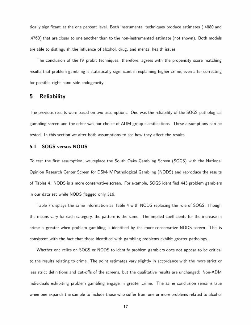
5 Reliability

The previous results were based on two assumptions: One was the reliability of the SOGS pathological

gambling screen and the other was our choice of ADM group classifications. These assumptions can be

tested. In this section we alter both assumptions to see how they affect the results.

5.1 SOGS versus NODS

To test the first assumption, we replace the South Oaks Gambling Screen (SOGS) with the National

Opinion Research Center Screen for DSM-IV Pathological Gambling (NODS) and reproduce the results

of Tables 4. NODS is a more conservative screen. For example, SOGS identified 443 problem gamblers

in our data set while NODS flagged only 316.

Table 7 displays the same information as Table 4 with NODS replacing the role of SOGS. Though

the means vary for each category, the pattern is the same. The implied coefficients for the increase in

crime is greater when problem gambling is identified by the more conservative NODS screen. This is

consistent with the fact that those identified with gambling problems exhibit greater pathology.

Whether one relies on SOGS or NODS to identify problem gamblers does not appear to be critical

to the results relating to crime. The point estimates vary slightly in accordance with the more strict or

less strict definitions and cut-offs of the screens, but the qualitative results are unchanged: Non-ADM

individuals exhibiting problem gambling engage in greater crime. The same conclusion remains true

when one expands the sample to include those who suffer from one or more problems related to alcohol

17

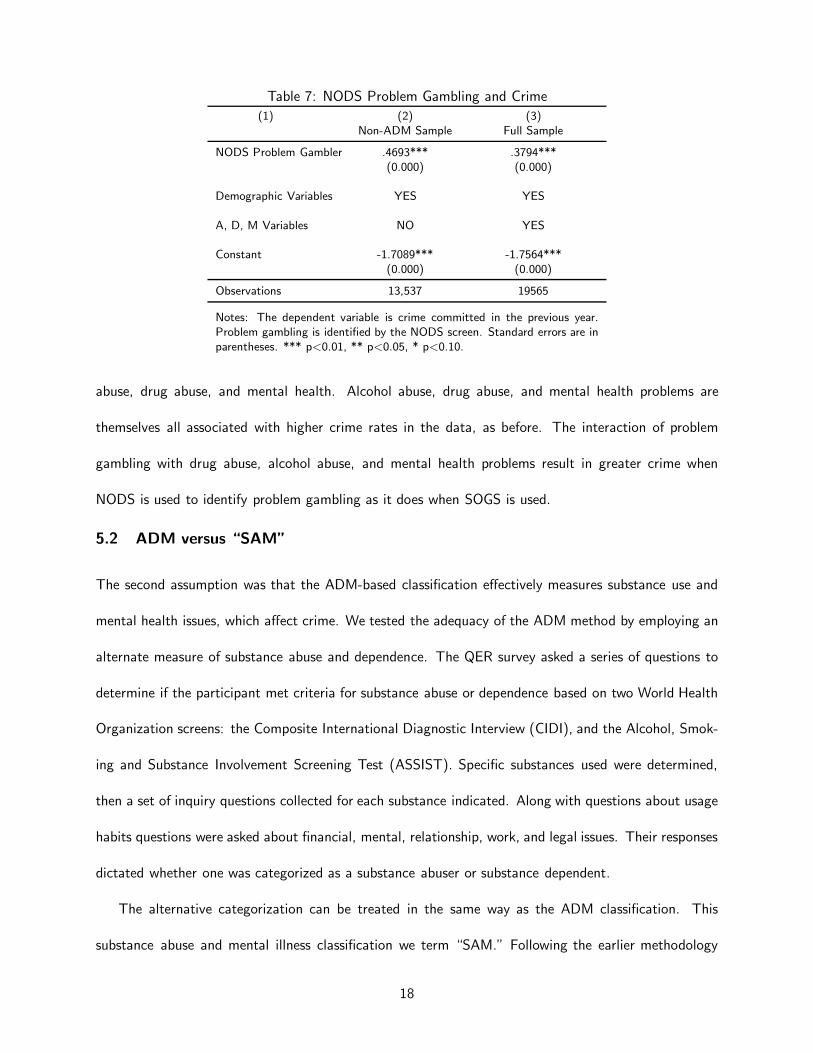
Table 7: NODS Problem Gambling and Crime

(1) (2) (3)Non-ADM Sample Full Sample

NODS Problem Gambler .4693*** .3794***(0.000) (0.000)

Demographic Variables YES YES

A, D, M Variables NO YES

Constant -1.7089*** -1.7564***(0.000) (0.000)

Observations 13,537 19565

Notes: The dependent variable is crime committed in the previous year.Problem gambling is identified by the NODS screen. Standard errors are inparentheses. *** p<0.01, ** p<0.05, * p<0.10.

abuse, drug abuse, and mental health. Alcohol abuse, drug abuse, and mental health problems are

themselves all associated with higher crime rates in the data, as before. The interaction of problem

gambling with drug abuse, alcohol abuse, and mental health problems result in greater crime when

NODS is used to identify problem gambling as it does when SOGS is used.

5.2 ADM versus “SAM”

The second assumption was that the ADM-based classification effectively measures substance use and

mental health issues, which affect crime. We tested the adequacy of the ADM method by employing an

alternate measure of substance abuse and dependence. The QER survey asked a series of questions to

determine if the participant met criteria for substance abuse or dependence based on two World Health

Organization screens: the Composite International Diagnostic Interview (CIDI), and the Alcohol, Smok-

ing and Substance Involvement Screening Test (ASSIST). Specific substances used were determined,

then a set of inquiry questions collected for each substance indicated. Along with questions about usage

habits questions were asked about financial, mental, relationship, work, and legal issues. Their responses

dictated whether one was categorized as a substance abuser or substance dependent.

The alternative categorization can be treated in the same way as the ADM classification. This

substance abuse and mental illness classification we term “SAM.” Following the earlier methodology

18

observations were divided into mutually exclusive and exhaustive groups fitting into one of four cat-

egories: no-substance-abuse-no-mental-health-issues (Non-SAM), substance-abuse-no-mental-health-

issues (SA), mental-health-issues-no-substance-abuse (M), substance-abuse+mental-health-issues (SAM).

The column (2) probit models used in Tables 4 and 7 were re-run using the new SAM classifications

and pathological gambler classifications generated by the original SOGS screen and by the alternative

NODS screen.

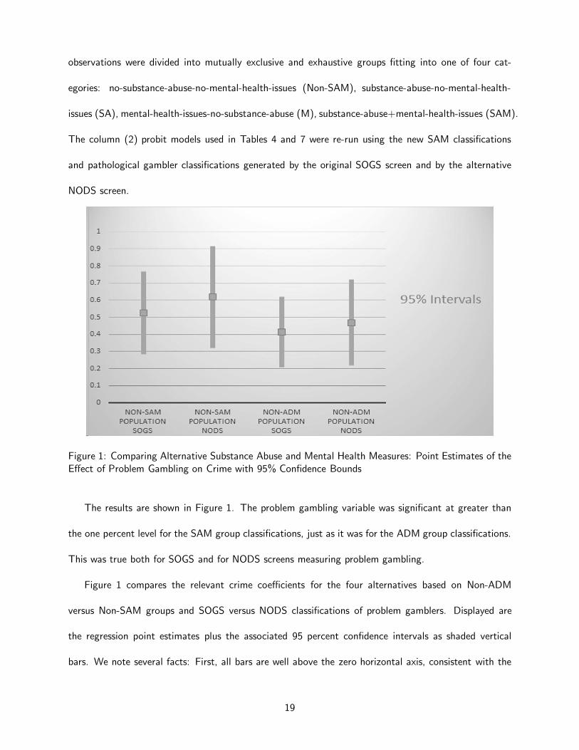
Figure 1: Comparing Alternative Substance Abuse and Mental Health Measures: Point Estimates of theEffect of Problem Gambling on Crime with 95% Confidence Bounds

The results are shown in Figure 1. The problem gambling variable was significant at greater than

the one percent level for the SAM group classifications, just as it was for the ADM group classifications.

This was true both for SOGS and for NODS screens measuring problem gambling.

Figure 1 compares the relevant crime coefficients for the four alternatives based on Non-ADM

versus Non-SAM groups and SOGS versus NODS classifications of problem gamblers. Displayed are

the regression point estimates plus the associated 95 percent confidence intervals as shaded vertical

bars. We note several facts: First, all bars are well above the zero horizontal axis, consistent with the

19

statistical significance at the one percent level or better for each coefficient. Second, as we found earlier,

the effect of NODS problem gambling on increased crime is greater than the effect of SOGS problem

gambling. We expect the NODS coefficients to be systematically larger than the SOGS coefficients

because it is designed to be a more conservative and more restrictive screen. If you are a problem

gambler as identified by NODS, you are more likely to engage in criminal activity. Third, all point

estimates are similar to one another, and lie within the confidence bounds of each of the others.

In summary, our reliability checks show robustness with respect to changes in the measure of problem

gambling used, with respect to changes in the measure of substance abuse and mental illness used, and

with respect to the point estimates of the variable of interest which is the impact of problem gambling

as a cause of crime.

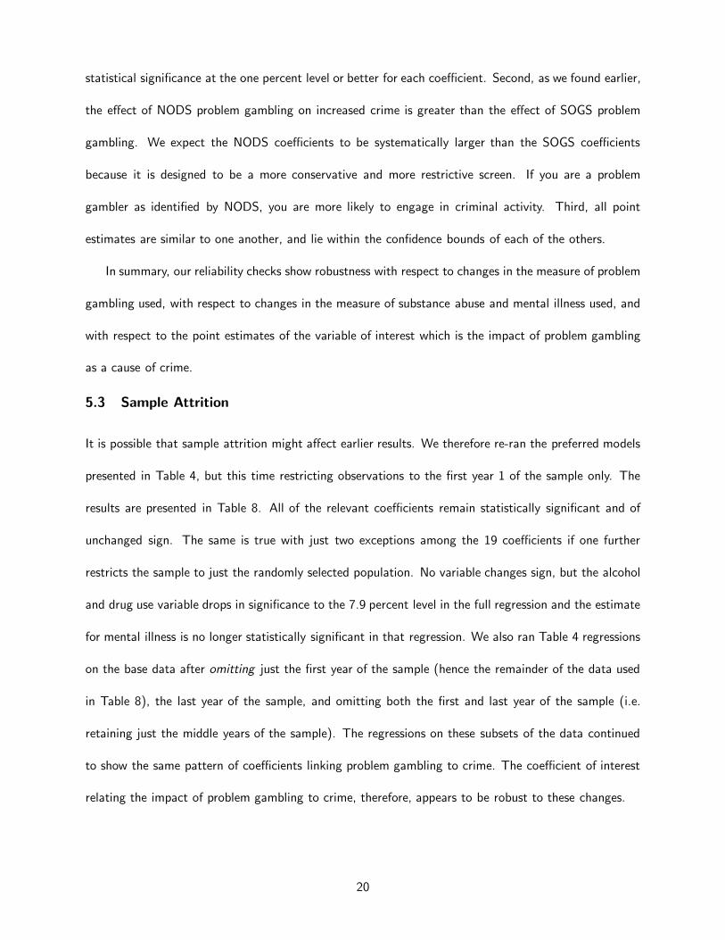
5.3 Sample Attrition

It is possible that sample attrition might affect earlier results. We therefore re-ran the preferred models

presented in Table 4, but this time restricting observations to the first year 1 of the sample only. The

results are presented in Table 8. All of the relevant coefficients remain statistically significant and of

unchanged sign. The same is true with just two exceptions among the 19 coefficients if one further

restricts the sample to just the randomly selected population. No variable changes sign, but the alcohol

and drug use variable drops in significance to the 7.9 percent level in the full regression and the estimate

for mental illness is no longer statistically significant in that regression. We also ran Table 4 regressions

on the base data after omitting just the first year of the sample (hence the remainder of the data used

in Table 8), the last year of the sample, and omitting both the first and last year of the sample (i.e.

retaining just the middle years of the sample). The regressions on these subsets of the data continued

to show the same pattern of coefficients linking problem gambling to crime. The coefficient of interest

relating the impact of problem gambling to crime, therefore, appears to be robust to these changes.

20

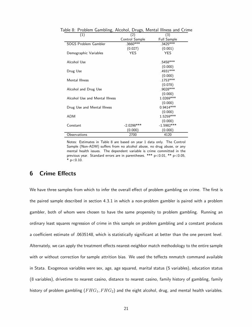
Table 8: Problem Gambling, Alcohol, Drugs, Mental Illness and Crime(1) (2) (3)

Control Sample Full Sample

SOGS Problem Gambler .3660*** .3425***(0.027) (0.001)

Demographic Variables YES YES

Alcohol Use .5458***(0.000)

Drug Use .4931***(0.000)

Mental Illness .1753***(0.078)

Alcohol and Drug Use .9028***(0.000)

Alcohol Use and Mental Illness 1.0269***(0.000)

Drug Use and Mental Illness 0.9414***(0.000)

ADM 1.5259***(0.000)

Constant -2.0298*** -1.5982***(0.000) (0.000)

Observations 2700 4120

Notes: Estimates in Table 8 are based on year 1 data only. The ControlSample (Non-ADM) suffers from no alcohol abuse, no drug abuse, or anymental health issues. The dependent variable is crime committed in theprevious year. Standard errors are in parentheses. *** p<0.01, ** p<0.05,* p<0.10.

6 Crime Effects

We have three samples from which to infer the overall effect of problem gambling on crime. The first is

the paired sample described in section 4.3.1 in which a non-problem gambler is paired with a problem

gambler, both of whom were chosen to have the same propensity to problem gambling. Running an

ordinary least squares regression of crime in this sample on problem gambling and a constant produces

a coefficient estimate of .0635148, which is statistically significant at better than the one percent level.

Alternately, we can apply the treatment effects nearest-neighbor match methodology to the entire sample

with or without correction for sample attrition bias. We used the teffects nnmatch command available

in Stata. Exogenous variables were sex, age, age squared, marital status (5 variables), education status

(8 variables), drivetime to nearest casino, distance to nearest casino, family history of gambling, family

history of problem gambling (FHG1, FHG2) and the eight alcohol, drug, and mental health variables.

21

Using the entire sample (valid if there is no attrition bias) produces an average treatment effect estimate

of .0428018 with a P-value of 0.000. Using just the first year randomly selected sample population (this

removes the possibility of sample selection bias and of attrition bias) produces an average treatment

effect estimate of .0763458 with P-value of 0.045. These three estimates suggest that crime is higher by

a number in the range between 4.28 to 7.63 percentage points (428 and 763 basis points), respectively,

due to the presence of problem gambling.

From these estimates we can infer the impact of the presence of casino (Class III) gambling on crime

if we have a base crime rate, a base problem gambling rate and an estimate of its rise when gambling is

adopted. In the random sampled portion of our data, the share of observations associated with problem

gambling is 3.44 percent, and the share of observations reporting having committed a crime when no

problem gambling is present is 3.54 percent. The earliest estimate of the prevalence of problem gambling

in the general population in the United States was 0.77 percent when the only casinos available were in

Nevada.8

We are able to perform the following armchair calculation: Presume that problem gambling rises

from .77 percent of the population to 3.44 percent when casino gambling changes from no availability

to availability 105 km away as in the Quinte population. Assume also that the prevalence of crime rises

from 3.54 percent of the population if they are non-problem gamblers to (3.54 + x) percent if they

are problem gamblers, where x is between 4.28 and 7.63. Now compare the number of crime incidents

for 100,000 population consisting of the appropriate proportion of problem gamblers and non-problem

gamblers in the two situations of casino availability. One finds that crime rises by 3.2 to 5.6 percent.

If the base rate estimate of problem gambling is reduced to 0.5 percent or raised to 1.0 percent, the

associated ranges become (3.5-6.3) or (2.9-5.1), respectively, in each case centering somewhere in the

4 percent range.

8Commission on the Review of the National Policy Toward Gambling, 1976, p. 73: “As a result of this clinicalexamination, it was estimated that 0.77 percent of the national sample could be classified as ‘probable’ compulsive gamblers,with another 2.33 percent as ’potential’ compulsive gamblers.”

22

We began this paper by reporting that counties that open casinos have crime rates about 8 percentage

points higher than their counterparts that do not open a casino. Collar counties in the cited study had

higher crime rates by about half this rate. Since the nearest casino in the present study was 105 km

distant, its crime effect of 3.2-5.6 is comparable to the collar county estimate found earlier and gives

some assurance of the reasonableness of the estimates found.

It is a short step to derive social cost estimates, and from them policy recommendations, by finding

cost figures for crime as a whole and charging 3.2 to 5.6 percent of this to the presence of casino

gambling and associated problem gambling, where the availability matches the distances of this study.

7 Conclusions and Implications

Researchers identify ten forms of gambling-related social consequences,9 the most prominent of which

is crime. Increased access to gambling lowers its cost to the user, increases the number of gamblers and

raises the number of problem gamblers.

Our research suggests that even at a distance of 105 km from the nearest casino, problem gambling

is associated with elevated crime. The estimates reported here suggest that problem gamblers commit

2.2 to 3.2 times the crime of a non-problem gambler.10 Our estimates suggest that the availability of

casino and racino gambling in the Quinte area is responsible for a 3.2-5.6 percentage point rise in crime.

This agrees with Grinols and Mustard (2006) who found that crime was on the order of 8 percentage

points higher in the counties themselves with operating casinos older than 3-4 years due to the casino

presence, with elevated crime roughly half that rate in the neighboring counties. Quinte is comparable

to a neighboring location.

9See, for example, New Hampshire Gaming Study Commission, 2010: Crime (eg. apprehension, adjudication, incarcer-ation, corrections), Business and Employment Costs (eg. lost productivity, job termination, lost work days), Bankruptcy,Illness (eg. stress-related illness, mental illness), Suicide, Social Service Costs (eg. welfare, treatment costs, unemployment-related costs), Regulatory Costs (eg. government oversight expenditures), Family Costs (eg. divorce, spousal separation,child abuse and neglect, domestic violence), Abused Dollars (eg. money inappropriately acquired from family, friends, oremployer that would be a crime but is not reported), Social Connections (eg. reduction of social capital), Political Costs(eg. increase in economic power resulting in disproportionate political influence). “Theoretically, many of these impactshave a financial cost to society one way or another and should be considered in an evaluation of the costs and benefits ofexpanded gambling (p. 48).”

10(3.54+x)/3.54 = 2.2 to 3.2 where x = 4.28 to 7.63.

23

As explained in the introduction, quality data on the effects of problem gambling is difficult to obtain

and mostly non-existent with respect to complicating “comorbid” factors. The present study therefore

provides a unique first look into the impacts of this singular activity on what many view to be the

most significant of gambling social costs. Problem gambling is linked to higher crime; its effect remains

even after accounting for complicating factors; and it shows up in non-parametric as well as parametric

indicators. On a preponderence of evidence basis, the conjecture that increased problem gambling leads

to higher crime is confirmed in our data.

We close by touching just briefly on the policy relevance of our results. State-sponsored gambling

has come to be viewed in many quarters as a tax collection device. At the same time, state-sponsored

regulated-monopolies for the purpose of raising public dollars raises policy concerns. First, such action

represents a controversial insertion of the state into a private market and what has traditionally been

the role of the private sphere. Second, such choices raise the question as to whether this is the best

way for government to raise revenues. To answer this question, we must be able to compare the social

costs of raising taxes by conventional means to the alternative “tax-by-gambling.” This paper provides

information relevant to the second question.

Appendix: Definitions of Gambling

The following definitions are from 25 U.S. C. 2703: (6)-(8):

(6) The term ”class I gaming” means social games solely for prizes of minimal value or

traditional forms of Indian gaming engaged in by individuals as a part of, or in connection

with, tribal ceremonies or celebrations.

(7) (A) The term ”class II gaming” means -

(i) the game of chance commonly known as bingo (whether or not electronic, computer,

or other technologic aids are used in connection therewith) -

(I) which is played for prizes, including monetary prizes, with cards bearing numbers or

24

other designations,

(II) in which the holder of the card covers such numbers or designations when objects,

similarly numbered or designated, are drawn or electronically determined, and

(III) in which the game is won by the first person covering a previously designated

arrangement of numbers or designations on such cards, including (if played in the same

location) pull-tabs, lotto, punch boards, tip jars, instant bingo, and other games similar to

bingo, and

(ii) card games that -

(I) are explicitly authorized by the laws of the State, or

(II) are not explicitly prohibited by the laws of the State and are played at any location

in the State, but only if such card games are played in conformity with those laws and

regulations (if any) of the State regarding hours or periods of operation of such card games

or limitations on wagers or pot sizes in such card games.

(B) The term ”class II gaming” does not include

(i) any banking card games, including baccarat, chemin de fer, or blackjack (21), or

(ii) electronic or electromechanical facsimiles of any game of chance or slot machines of

any kind.

(C) Notwithstanding any other provision of this paragraph, the term ”class II gaming”

includes those card games played in the State of Michigan, the State of North Dakota, the

State of South Dakota, or the State of Washington, that were actually operated in such

State by an Indian tribe on or before May 1, 1988, but only to the extent of the nature and

scope of the card games that were actually operated by an Indian tribe in such State on or

before such date, as determined by the Chairman.

(D) Notwithstanding any other provision of this paragraph, the term ”class II gaming”

includes, during the 1-year period beginning on October 17, 1988, any gaming described in

25

subparagraph (B)(ii) that was legally operated on Indian lands on or before May 1, 1988,

if the Indian tribe having jurisdiction over the lands on which such gaming was operated

requests the State, by no later than the date that is 30 days after October 17, 1988, to

negotiate a Tribal-State compact under section 2710(d)(3) of this title.

(E) Notwithstanding any other provision of this paragraph, the term ”class II gaming”

includes, during the 1-year period beginning on December 17, 1991, any gaming described

in subparagraph (B)(ii) that was legally operated on Indian lands in the State of Wisconsin

on or before May 1, 1988, if the Indian tribe having jurisdiction over the lands on which

such gaming was operated requested the State, by no later than November 16, 1988, to

negotiate a Tribal-State compact under section 2710(d)(3) of this title.

(F) If, during the 1-year period described in subparagraph (E), there is a final judicial

determination that the gaming described in subparagraph (E) is not legal as a matter of

State law, then such gaming on such Indian land shall cease to operate on the date next

following the date of such judicial decision.

(8) The term ”class III gaming” means all forms of gaming that are not class I gaming

or class II gaming.

References

Australian Productivity Commission. 1999. Australia’s Gambling Industries. (Vols. 1-2). Report no.

10. Canberra: Australian Capital Territory.

Babor, Thomas F., Robert S. Stephens, and G. Alan Marlatt. 1987. Verbal Report Methods in Clinical

Research on Alcoholism: Response Bias and its Minimization. Journal of Studies on Alcohol, 48:

410-424.

26

Baum, Christopher F. 2012. sspecialreg: Stata module to estimate binary choice model with discrete en-

dogenous regressor via special regressor method. http://ideas.repec.org/c/boc/bocode/s457546.html

Blaszczynski, Alex and Zachary Steel. 1998. Personality disorders among pathological gamblers. Journal

of Gambling Studies, 14 (1): 51-71.

Commission on the Review of the National Policy Toward Gambling. 1976. “Gambling in America,”

Final Report. Washington, DC: US Government Printing Office.

Dehejia, Rajeev H. and Sadek Wahba. 2002. Propensity Score-Matching Methods for Nonexperimental

Causal Studies, The Review of Economics and Statistics, 84 (1): 151-161.

Dickerson, Mark G. Ellen Baron, Sung-Mook Hong, and David Cottrell. 1996. “Estimating the extent

and degree of gambling related problems in the Australian population: A national survey.” Journal

of Gambling Studies, 12: 161-178.

Gerstein, Dean, John Hofmann, Cindy Larison, Laszlo Engelman, Sally Murphy, Amanda Palmer, Lu-

cian Chuchro, Marianna Toce, Robert Johnson, Tracy Buie, Mary Ann Hill, Rachel Volberg, Henrick

Harwood, Adam Tucker, Eugene Christiansen, Will Cummings, and Sebastian Sinclair. 1999. “Gam-

bling Impact and Behavior Study: Report to the National Gambling Impact Study Commission,”

National Gambling Impact Study Commission, (1 April).

Grinols, Earl L. and David B. Mustard. 2006. Casinos, Crime, and Community Costs, The Review of

Economics and Statistics, 88 (1), February: 28-45.

Grinols, Earl L. 2004. Gambling in America: Costs and Benefits. New York: Cambridge University

Press.

2007. Social and Economic Impacts of Gambling. In Research and Measurement Issues

in Gambling Studies, edited by DG Smith, D Hodgins, and DR Williams. Amsterdam: Else-

vier/Academic Press: 515-537.

27

Gupta, Rina and Jeffrey L. Derevensky. 1997. Familial and social influences on juvenile gambling.

Journal of Gambling Studies, 13 (3): 179-192.

Jaret, P. and B. Hogan, “A Desparate Gamble, AARP Bulletin, January-February, 2014,24-28. Grinols

and Mustard (2006), p.32 provide other examples.

Lesieur, Henry R. 1984. The Chase: Career of the Compulsive Gambler. Schenkman Books, Cambridge.

Lewbel, Arthur and Susanne M. Schennach. 2007. A Simple Ordered Data Estimator for Inverse Density

Weighted Functions. Journal of Econometrics, 136 (1): 189-211.

Narayanan, Sridhar and Puneet Manchanda. 2012. An Empirical Analysis of Individual Level Casino

Gambling Behavior. Quantitative Marketing And Economics, 10 (1): 27-62.

National Research Council. 1999. “Social and Economic Effects” in Pathological Gambling: A Critical

Review. Washington, DC: The National Academies Press.

New Hampshire Gaming Study Commission. 2010. Analyzing the Impact of Expanded Gambling on

New Hampshire: Final Report of Findings, May: 1-69.

Potenza, Marc N. 2008. The Neurobiology of Pathological Gambling and Drug Addiction: An Overview

and New Findings. Philosophical Transactions: Biological Sciences, 363(1507): 3181-3189.

Roese, Neal J. and David W. Jamieson. 1993. Twenty years of bogus pipeline research: A critical

review and meta-analysis. Psych Bulletin, 114: 363-375.

Shaffer, Howard J. and David A. Korn. 2002. Gambling and related mental disorders: A public health

analysis. Annual Review of Public Health, 23: 171-212.

Stinchfield, Randy and Ken C. Winters. 1998. Gambling and Problem Gambling Among Youths. Annals

of the American Academy of Political and Social Science, 556: 172-185.

Volberg, Rachel A. 1994. The prevalence and demographics of pathological gamblers: implications for

public health. American Journal of Public Health, 84: 237-241.

28

Williams, Robert J. and Nadine Nowatzki. 2005. Validity of adolescent self-report of substance use.

Substance Use and Misuse, 40(3): 1-13.

Williams, Robert and Robert Hann. 2006. “Examining the Impact of a Race Track Slots Facility

in the Belleville, Ontario Area.” February 24, 2006 Research Proposal submitted to the Ontario

Problem Gambling Research Centre. Robert Williams and Robert Hann, principal investigators;

co-investigators Donald Schopflocher, Robert Wood; consultants Earl L. Grinols, Jan McMillen.

Term of project April 1, 2006–February 28, 2012.

29