Louisiana State UniversityLSU Digital Commons

LSU Historical Dissertations and Theses Graduate School

1957

Problems in the Application of Statistical QualityControl to a Manufacturing Plant.Chung Wei ChenLouisiana State University and Agricultural & Mechanical College

Follow this and additional works at: https://digitalcommons.lsu.edu/gradschool_disstheses

This Dissertation is brought to you for free and open access by the Graduate School at LSU Digital Commons. It has been accepted for inclusion inLSU Historical Dissertations and Theses by an authorized administrator of LSU Digital Commons. For more information, please contactgradetd@lsu.edu.

Recommended CitationChen, Chung Wei, "Problems in the Application of Statistical Quality Control to a Manufacturing Plant." (1957). LSU HistoricalDissertations and Theses. 196.https://digitalcommons.lsu.edu/gradschool_disstheses/196

COPYRIGHTEDby

CHUNG WEI CHEN 1957

PROBLEMS IN THE APPLICATION OF STATISTICAL QUALITY CONTROL TO A MANUFACTURING PLANT

A Dissertation

Submitted to the Graduate Faculty of the Louisiana State University and

Agricultural and Mechanical College in partial fulfillment of the requirements for the degree of

Doctor of Philosophyin

The Department of Business Administration

byChung Wei Chen

B. A., National Chengchi University, 194& Licenci^ en Droit, National Chengchi University, 19ifS

M. B. A., Louisiana State University, 1954June, 1957

ACKNOWLEDGMENT

The writer wishes to express his gratitude to Dr.P. F. Boyer, Professor of Business Administration and Director of the Division of Research, Dr. H. L. McCracken, Professor of Economics, Dr. W. H. Baughn, Professor of Business Administration, Dr. S. W. Preston, Professor of Business Administration, Dr. W. D. Ross, Professor of Economics and Dean of College of Coinnerce, Dr. H. E.Bice, and Dr. L. C. Megginson, Associate Professor of Business Administration, for their advice and assistance during the preparation of this dissertation.

ii

TABLE OF CONTENTSPage

ACKNOWLEDGMENT............................................ iiTABLE OF CONTENTS...........................................iiiLIST CF FIGURES.......................................... Iv

LIST OF SCHEDULES....................................... vLIST OF TABLES............................................ viLIST OF CHARTS............................................. viii

ABSTRACT................................................... xCHAPTER

I. INTRODUCTION...................................... 1II. PRINCIPLES AND METHODS OF STATISTICAL QUALITY

CONTROL........................................ 6III. ORGANIZATION AND MANUFACTURING PROCESS OF A WAR

PRODUCT PLANT........... 21IV. ORGANIZATIONAL STRUCTURE OF STATISTICAL QUALITY

CONTROL GROUP.................................. 36V. APPLICATION OF STATISTICAL QUALITY CONTROL TO

PLANT D ........................................ 50VI. SUMMARY AND CONCLUSIONS........................... 103

SELECTED BIBLIOGRAPHY .................................... 107VITA.......................................................... Ill

ill

LIST OF FIGURES

Figure Page

1 Organizational Structure of Plant D.......... 232a Advisory Pattern - Statistical Quality

Control Group Placed in the Inspection Department. ...... 3 7

2b Advisory Pattern - Statistical QualityControl Group Placed in the Engineering Department................................. 33

2c Advisory Pattern - Statistical QualityControl Group Placed Directly Subordinate to the Plant Manager................. 40

3 Departmental Organization. . . . . . . . . . ^31+ Authoritative Pattern.................. ..

iv

LIST OF SCHEDULES

Schedule

1o

Page

Factory Operation......... . ............... Z'

Inspection List. . 31

v

LIST OF TABLES

Table1

3

k

6

7

10

1112

13

Ik

Measurements of Base ThicknessResults of Observations in Table 1 Scored

to Form Frequency Distributions • . . .Calculation of Standard Deviation for Base

Thickness............... • • .............Measurements of Diameter of Recess GrooveMeasurements of Diameter of Recess Groove,

After Resetting Adjusted with a Master piece ......... ..

Measurements of Diameter of Recess Groove, Produced by Trouble Free Machines . . .

Measurements of Diameter of Recess Gr ove, After Improvement........... ..

Measurements of Length from Base to Rear Band .................. ..

Measurements of Length from Base to Rear Band, Produced by Trouble Free Machines

Measurements of Length from Base to Rear Band, After Improvement ......... . . .

Measurements of Diameter of Band Seat . .Measurements of Diameter tf Band Seat,

Produced by Trouble Free Machines . . .Computation of Trial Control Limits for

Control Chart for Per Cent Defective in Diameter of Bourrelet . . . . .........

Computation of Trial Control Limits for Control Chart for Per Cent Defective of Recess Groove . . . . . . . . .........

Page61

-k

6566

69

72

B1

Bi+f>7

90

93

or

vi

Table Page17 Computation of Trial Control Limits for

Control Chart for Per Cent Defective inLencth from Base to Rear B a n d .............. 97

16 Computation of Trial Control Limits forControl Chart for Fer Cent Defective inProfile of Boat-Tail................. 99

IB Computation of Trial Control Limits forControl Chart for Per Cent Defective inBase Cover 7/eld........................ • . • 101

vii

LIST OF CHARTS

Chart Page1 X-Chart for Base Thickness....................2 R-Chart for Base Thickness............. 633 X-Chart for Diameter ' f Recess Groove . . . . 6?i+ R-Chart for Diameter of Recess Groove . . . . 635 X-Chart for Diameter of Recess Groove, After

Resetting Adjusted with a Master Piece. . . 70R-Chart for Diameter of Recess Groove, After

Resetting Adjusted with a Master Piece. . . 717 X-Chart for Diameter of Recess Groove,

Produced by Trouble Free Machines.......... 733 R-Chart for Diameter of Recess Groove,

Produced by Trouble Free Machines.......... 749 X-Chart for Diameter of Recess Groove, After

Improvement . ................ . . . . . . . ?610 R-Chart for Diameter of Recess Groove, After

Improvement . . . . . ...................... 7711 X-Chart for Length from Base to Rear Band . . 7912 R-Chart for Length from Base to Rear Band . . 3013 X-Chart for Length from Base to Rear Band,

Produced by Trouble Free Machines . . . . . 3214 R-Chart for Length from Base to Rear Band,

Produced by Trouble Free Machines . . . . . 3315 X-Chart for Length from Base to Rear Band,

After Improvement .................... 3516 R-Chart for Length from Base to Rear Band,

After Improvement..................... 36

viii

Chart Page17 X-Chart for Diameter of Band Seat.............IB R-Chart for Diameter of Band Seat.......... B919 X-Chart for Diameter of Band Seat, Produced by

Trouble Free Machines............. 91SO R-Chart for Diameter of Band Seat, Produced by

Trouble Free Machines. ............. 9221 p-Chart for Diameter of Bourrelet.......... .. 922 p-Chart for Diameter of Recess Groove..... of

23 p-Chart for Length from Base to Rear Band. . . 9BZh p-Chart for Profile of Boat-Tail........... . loo25 p-Chart for Base Cover Weld.......... 102

ix

ABSTRACT

The purpose of this dissertation is to study the ad­vantages of statistical quality control in a war product plant, to set up a theoretical organization operating in the plant, and to apply statistical methods to quality control of the manufactured products.

The introduction gives the fundamental change in the concept of inspection, the historical development of statistical quality control to modern manufacturing plants.

A discussion of general principles and methods of statistical quality control and a review of the convention­al methods of control charts for variables are presented.

A study was made of the organization and manufacturing process of a plant with an idea of applying statistical quality control principles. This war product plant has not applied statistical quality control but has used one- hundred per cent inspections at many points to screen out the defective goods. This practice i3 limited by the psychological law of diminishing efficiency. An application of statistical quality control in the plant would result in a saving of the excessive cost of inspection and would guarantee an improvement in quality.

Applications of statistical quality control to modern manufacturing plants are important; also important is a suitably organized statistical quality control group in the plant. The presentation of various existing organizational patterns provides a means for the comparison of their ad­vantages as well as their disadvantages. The most ad­vantageous organization of a statistical quality control group in a modern manufacturing company is suggested as the authoritative pattern, although it ha3 not yet been used. Consideration has been given to the size of the war product plant in devising a statistical quality control group that is held to be suitable to the operation of that plant,

A practical application of statistical quality control is made in connection with some of the work done in the war product plant. The over-all rate of rejection in that plant has always been high, but difficulties leading to rejections are by no means experienced in all parts of the plant’s production. This discovery points to the need for reducing over-all inspection and for concentrating attention on the seriously troublesome parts. Some of the most serious production problems in the manufacturing process are analyzed; assignable causes are detected; and corrective actions are suggested. Managerial conclusions are reached regarding the organization, manufacturing process, and in­spection methods.

xi

CHAPTER I INTRODUCTION

Many years ago, the achievement of standardization in industry led to interchangeability which, in turn made mass production possible. Methods involved in standard­ization were primarily dependent upon inspection. The concept of inspection was implemented by the comparative­ly simple procedure of separating good items from bad ones in order to find the "exact likeness" of products.

It was not until about 1540 that the concept of a "go" tolerance limit was introduced and not until about 1570 that the "go, no-go" tolerance limits were first used.^ The use of this principle of separating the "bad" from the "good" continued to dominate the production process until recent years.

In 1924, Walter A. Shewhart applied statistical2methods to quality control and developed control charts.

^Walter A, Shewhart, Statistical Method from the Viewpoint of Quality Control (Washington: The GraduateSchool, The Department of Agriculture, 1939 ), p» 2.

2Acheson J. Duncan, Quality Control and Industrial Statistics (Homewood, Illinois: Richard D. Irwin, Inc.,1952), p. 1.

These applications and developments have done much to bring about some fundamental changes in the concept of producing to specification.

Inherent variability is present In all things. The presence of that inherent variability prevents us from making exact duplicates. The early concept of inspection to find the matching parts, or parts conforming to specifi­cation, worked fairly well. The device of the "go" gauge gives either the upper or the lower tolerance. The intro­duction of the "go, no-go" gauge fixes both the upper and lower tolerance. however, neither of these devices can be used extensively for the purpose of analyzing the causes of quality variation.

Statistical quality control is the tool which enables us to find If a stable pattern of variation exists, to learn when and where a change in the pattern of variation arises, and to tell us when a process requires corrective actions. A wise use of this tool promises to improve the quality of products, to reduce rejections to a minimum, to warn of impending troubles, to reduce costs of inspection and of production, to narrow tolerances, and to provide a better basis for establishing or altering specification requirements.

Although, in the past 30 years, principles and methods of statistical quality control have been developing rapidly,

3

applications of statistical methods to quality control of manufactured products are, as yet, U3cdto a very limited extent, especially in the southern states. The reasons for thi3 limited application do not attach to the principle of statistical quality control itself. Instead, the efforts of a broad program of education for managerial personnel in techniques of statistical quality control are necessary If plant managers are to understand the advantages of utilizing this new tool.

Certain kinds of manufacturing plants do not as yet utilize the principles of statistical quality control. This fact cannot be explained in terms of any objections to the principles of such control or of any limitations of their application to those fields of manufacturing. Some plant managers do not recognize the advantages of the application of statistical quality control. Instead, they rely entirely upon their traditional one-hundred per cent inspection method.

With this fact in mind, the writer introduces applica­tions of statistical quality control to a plant which not only does not U3e methods of statistical quality control, but which is one of a type of plants in which no such methods have been used. It Is the purpose of this dissertation to study the advantages of statistical quality control to the manufacturing plant, to set up a theoretical organization operating in the plant, and to apply statistical methods to the quality control of manufactured products.

The plant with which this survey is specifically con­cerned deals exclusively with governmental orders. It produces a kind of war material. For obvious reasons the name of the plant is held confidential. Likewise, the writer will, so far as is practicable, avoid the use of terms which refer to the parts of the product and to the classifications of defects that are used by the Government.

Although the plant does not utilize statistical quality control, its finished products are subject to an acceptance or a rejection based upon statistical standards specified by the Government. Furthermore, the Government rates plants of this kind by the use of statistical quality control methods. For these reasons, the use of statistical methods is especially important in this kind of plant.

Since symbols used In statistical literature are not fully standardized, the writer uses, in general, those employed by Eugene L. Grant in his work.^

The general principles and methods of statistical quality control will be included briefly in Chapter II. Chapter III will present the managerial organization and manufacturing process of the plant under survey. Chapter IV is to be devoted to the introduction of a theoretical

3Eugene L. Grant, Statistical Quality Control. Second edition. {New York: McGraw-Hill Book Company, Inc.,1952.)

statistical quality control program in the plant. Suitabl applications of statistical quality control methods to specific operations will be presented in Chapter V. The conclusions drawn from the results of this study will be found in Chapter VI.

CHAPTER IIPRINCIPLES AND METHODS OF STATISTICAL QUALITY CONTROL

Although the historical development of statistics Is as old as that of mathematics and statistics has been ap­plied to other fields for several centuries, the applica­tion of statistical methods to quality control Is relative­ly new. The first person to apply statistical methods to the problem of quality control was Walter A. Shewhart of the Bell Telephone Laboratories. Shewhart made the first sketch of a modern control chart In a memorandum prepared on May 16, 1924* In 1931» Shewhart published a book entitled Economic Control of Quality of Manufacturing Product. which set the pattern for subsequent applications of statistical methods to process control.

Two other Bell System men, H. F. Dodge and H. G. Romig, developed the application of statistical theory to sampling inspection and published their work in the now well-known Dodge-Romig Sampling Inspection Tables. Efforts of Shewhart, Dodge, and Romig constitute much of what today is the theory of statistical quality control.^

itDuncan, o£. cit.. p. 2.

6

7

Despite the rapid development of statistical methods for quality control, the rate of adoption has been very slow. According to H, A. Freeman, there were two major

n;reasons.' First, American production engineers believed that their principal function was to improve technical methods so that no important quality variations would remain, and that in any case, laws of chance would have no proper place among scientific production methods. The second reason was the difficulty of obtaining industrial statisticians who were adequately trained in this fairly complicated field. Eecause of these obstacles, in 1937 probably not more than a dozen enterprises in American mass-production industries had introduced the new technique into their ordinary opera­tions .

During World War XI, the armed services entered the market as large consumers. The armed services adopted statistical sampling inspection procedures and brought direct pressure on producers of war products to adopt sta­tistical quality control methods in order to meet require­ments of acceptance and to lower the rate of rejection of products.

In addition to direct pressure, an education and research program was carried on by the Government. Upon the

5H. A. Freeman, ’’Statistical Methods for Quality Control,” Mechanical Engineering. LIX(April, 1937), 261.

request of the War Department, the American Standards Associ ation initiated a project in December, 1940, covering the application of statistical methods to the quality control of materials and manufactured products. A series of pamphlets concerning quality control was published. The Office of Production Research and Development of the War Production Board established 33 intensive courses on sta­tistical quality control during the period 1943 to 191+5. Eight hundred and ten organizations sent representatives to attend one or more of these short courses.

Subsequent to the completion of the introductory courses, quality control societies were formed in various localities. On February 16, 1946, a national organization known as the American Society for Quality Control was formed It has become the leading force in promoting the use of statistical methods for quality control in American indus­tries.

From the United States, statistical quality control techniques spread geographically and increased considerably in scope. Quality control societies exist in Europe and the Far East. Other statistical techniques, such as correla­tion, analysis of variance, and the design of experiments, have been used in industrial laboratories and research departments.

Measured quality of manufactured products is always subject to a certain amount of variation as a result of

chance. Those processes which are characterized by a stable pattern of variation are said to be in statistical control, whereas those which are characterized by unstable patterns of variation are regarded as being statistically out of control.

Individual measurements of products may form a frequency distribution. In this device, individual measurements are classified into groups. The number of items falling into each group is stated. Although the formation of a frequency distribution sacrifices much industrial detail, It retains enough of the original characteristics f̂ f data for valuable analyses. There are two basic statistical measures of the frequency distribution: the measure of central tendency andthe measure of dispersion.

The most common measure of a central tendency is the arithmetic mean, or X, which Is the quotient of the sum of the individual values divided by the number of items. The second measure of a central tendency is the median, or Med. The median is defined as that value which divides a distri­bution so that an equal number of items are on either side of that value. The third measure of central tendency is the mode, or Mo, which is the value at the point around which the Items tend to be most heavily concentrated.

The most common measures of dispersion are the standard deviation and the range. The standard deviation, which is the abbreviated term of the standard deviation from the

arithmetic mean, is the square root of the average of the squared deviations of the individual values from the arith­metic mean. The Greek symbol 6 (small sigma) is used to represent it. The range, or R, is simply the difference between the largest and smallest values in a series.

For statistical quality control, mathematical statis­ticians have found that the best measure of central tendency is the arithmetic mean, and that the best measure of dis­persion is the standard deviation. Usually in practical control charts, the standard deviation is, however, not actually computed but estimated from the range.

A frequency distribution which is normally distributed forms a bell-shaped, symmetrical curve. Such a curve is referred to as a normal curve. According to Shewhart*s normal bowl, in the long run the grand mean will be the same as the mean of the universe, and the standard deviation of the frequency distribution of X values will be the standard deviation of the universe divided by the square root of the sample size. Even though the distribution in the universe is not normal, the distribution of the X values tends to be normal. The larger the sample size and the more nearly normal the universe, the closer will the frequency distribution of averages approach the normal curve.^ This

Grant, op. sit., p. 87.

fact Is very important in the application of control chartControl limits are developed from the principle that thefrequency of occurrence is proportional to the size of thearea under a normal curve. For example, 99.73 per cent ofthe area under a normal curve is included within the limitof * 3-sigma for the mean. The standards prepared by theBritish standards Institution use probability limits. TheAmerican standards on control charts use 3-sigma control

7limits.Control limits of control chart for X are set at thre

standard errors of the mean on either side of the grand mean. Since the standard deviation of the universe is estimated from the average range, R, and the standarddeviation of the universe has a constant ratio to thestandard error of the mean for a given size of sample, a multiplier of the average range designated as A0 i3 de­veloped. The formulae for calculating the 3-sigma control limits on the mean chart are a3 follows:

UCL-r - X ♦ 3 C - - X ♦ A RA X &

LCLy = » X - 3 * x = X - A2R

The spread of the distribution of standard deviations decreases as the size of the sample increases. The

7Ibld.. pp. 105-106

12

distribution of standard deviations is not symmetrical, whengthe size of sample is small. These facts limit the use of

control charts for standard deviation.When the universe is normal, a control chart for the

standard deviation may be used. The central line is set at the average of standard deviations of all subgroups. Con­trol limits are set at three standard deviations of the standard deviations on either side. The formulae are:

UCLf - g *

LCLt = % - 3^^ =

In practical statistical quality control work in indus­try, control charts for standard deviation are not often used. The establishment of control limits on control charts for the standard deviation is based on the assumption that the universe is normal. It has been realized that the dis­tribution of standard deviations Is not normal. Control charts for the standard deviation are complicated both in computation and interpretation, and hard to explain to personnel who have neither a mathematical nor a statistical background.

In lieu of the control chart for the standard deviation, the control chart for the range is often used in industry.

6Ibid.. pp. 100-101.

13

Not only is the ran^o easier to compute, but almost every­one can understand the meaning of it. Formulae for control limits of the control chart for the range are:

UCLd = D, R R k

i.c l r = l3r

When the size of a subgroup is six or less, equals zero. Thus, as long as the subgroup size is six or less, the lower control limit on the R-chart is always zero regardless of the value if R.

Shewhart suggested four as the ideal subgroup size. In the industrial use f control charts, five seems to be the most common size. Since the lower control limit on the R- chart is always zero when the subgroup size is six or less, the so-called central line on the R-chart is not real]y the middle line between the upper and the lower limits. When an increase in the universe dispersion occurs, more points will likely fall above the central line than below it. Such extreme runs cannot simply be interpreted as an evidence of lack of control. On the other hand, a decrease in the uni­verse dispersion cannot be reflected in points falling below the lower control limit on the R-chart.

Not all quality characteristics of manufactured products are capable of being measured. This fact limits the use of control charts to variables. Shewhart developed control

I k

charts f ,r attributes as a substitute for control charts for variables, when the latter is net applicable.

A record which shows only the number ~ f articles con­forming and the number of articles failing to conform to any specified requirements is said to be a record of attri­butes. When a record is made of an actually measured quality characteristic, such as a dimension expressed in thousandths of an inch r a weight expressed in hundredths of an ounce, the quality is said to be expressed in variables.

Control charts for attributes consist of p-chart, np- chart, and c-chart. The control chart for fraction defective is commonly referred to as the p-chart. Although the p-chart is less sensitive than the X- and R-charts, and does not have as great a diagnostic value, the p-chart is still a useful aid to production supervision and to quality control in giving information as to when and where to exert pressure for a possible quality improvement and to disclose erratic fluctu­ations in the quality of products. There is still another advantage in the use of the p-chart. Almost all manufacturing companies have some records of inspected items as to either accepted or rejected, even though they do not know the merit of statistical quality control. These records are helpful in estimating the process average. The estimated process average will serve as a guide to inspection, if the company decides to use statistical quality control.

I e;

Although the fraction defective nay vary considerably from sample to sample, the relative frequencies of various sample fractlon defectives may te expected to follow the binomial law, so lone; as the universe fraction defective mrains unchanged. The standard deviation of the fraction defective is;

For the purpose of computing trial control limits, p f is assumed to be the observed average fraction defective p. Therefore, the formulae for 3**sigma trial control limits on the p-chart ar*' :

When the universe fraction defective (p*) is known, it should be used instead of the average fraction defective (p) in the above formulae.

If the subgroup size is constant, a control chart for the actual number of defectives may be used. Such a chart is called the control chart for np or the np-chart. Three- sigma limits on the np-chart are;

LCLP “ P " 3*p - Pp - 3 - jp(l ~ p)n

16

LC1. = p - 3r- = P - Inp (1 - p)np « np

There are two reasons for preferring a np-chart to a p-chart: (1) The np-chart saves one calculation for eachsubgroup. (2) The managerial personnel may more easily understand the np-chart than the p-chart.

The control chart for defects is generally referred to as the c-chart. The c-chart applies only to a limited number of manufacturing situations involving quality. The control limits on the c-chart are based on the Poisson distribution. A defective is an article that in some way fails to conform to one or more given specifications, whereas a defect is referred to as each instance of the article's lack of conformity to specifications. bince a product may have a number of specifications or may be assembled from manj1’ parts, a product may have many defects. Furthermore, each defect may have a different average occurrence. A mathematical statistician developed the following generali­sation:^

”A frequency distribution will not follow the Poisson law if some of the frequencies recorded refer to the number of occurrences of one event that follows the Poisson law, and the remaining frequencies recorded refer to the number of oc­currences of another event that also follows the Poisson law but has a different average. But a frequency distribution will follow the Poisson law if a count is made of the combined number of occurrences of both events provided the pairing of the two events is at random."

9Ibid.. p. 270.

The standard deviation of the Poisson distribution is c.f , where cf is referred to as the standard value of the

av'Tagp number of defects per unit. The j-sigma limits on the c-chart are:

V/hen c* is not I-nown, the observed average number of defects per unit (c) ray substitute for cf in the above formulae.

In addition to these control charts, another statisti­cal t e c h n i q u e used in manufacture no; is t h e acceptance sampling plan. Jtrictly speaking, the acceptance sampling plan is not an attempt to control quality, but merely to accept or to reject lots. If lets arc all of the same quality, there may be some of thorn accepted and some of them rejected. In such a case, the accepted lots are not better than the rejected lots in regard to quality. T h e

chance for acceptance or rejection depends entirely upon the probability of occurrence. If lots are of a different quality, the better lots will be accepted more frequently than the poorer lots.

The theory of the acceptance sampling plan is based on the law of probability. According to the number of samples drawn before reaching a decision of whether to

UCL - c T +

accept or to reject the 1 t, th t accoptanc-' samp 2 5 ng plan '.ay be classi fi e'i as sin "7. ■ -, dou’le, n.ul tipi e ;r sequential samp! i n o plan.

In a single sampling plan, the ‘incision of whether to accept ->r to reject a "! :t is 'aseh on the evidence c f on! y one sample. In a doubl e >r mol tip1o sanpl inr pilar, a seconi saiuplf. is not always neo-ussary. If the first sar.pl r

appears good emuqh, the 1 ,1 is accepted. If t h e first sample appears bad enough, the let 's re j ̂>ct rd. An ad­ditional sample wil 1 br t a! ’ pr., only when th^ first sanpl e is neither pood enough nor had rnonfn. When two or no re samples are drawn, the Lied si on as te whether to accept or to reject is based on the «'viience of all samples taken.

According to the quality characteristics of products, the acceptance sampling: plan nay be classified as sampling by attributes and sampling by variables. The great ad­vantage of the use of acceptance sampling hy variables is that more information can be obtained from a sample about the quality characteristics than from; a sample showing merely the conforming and/or nonconforming articles. This advantage may lead to a number of desirable results, such as better quality protection, better basis for guidance toward quality improvement, better judgment for giving weight to the quality history in acceptance decisions, and easier discovery of errors .f measurements, as compared with the use of a plan based on attributes.

3?

There are, h'wever, s^mc disadvantages of the use of a plan eased on variables. one obvious limitation is the fact that many quality characteristics are observable only as attributes. Whenever this condition exists, sampling by variables is out of the question. The second limitation is the fact that acceptance criteria must be applied separately to each quality characteristic. Furthermore, frequency distributions of many industrial quality characteristics may not be normal. When the underlying frequency distribution is skewed, or even is symmetrical but either peaked or flat-topped, percentages in the extreme tails of such distri­bution may differ considerably from those obtained under a normal distribution. Thus, the protection against the stated percentage of defectives giv^n by acceptance criteria by variables may be either considerably greater or less than the protection indicated by the operating characteristic curves computed n the assumption of a normality of the distribution.

Whether a plan based on variables will save money will depend largely on the relative cost of dividing products into defective and effective categories, as compared with the cost of making quantitative measurements. If both methods of inspection are destructive, the acceptance cri­terion by variables is especially likely to be desirable.

The operating characteristic curve which is referred to as the OC curve is useful in evaluating an acceptance

sampling plan. The OC curve is based on the law of proba­bility and shows the probability of acceptance, Pa, by the sampling plan of any submitted lot having a fraction de­fective p. The steeper the slope of the OC curve, the greater is its ability to screen bad lots* The best OC curve is, therefore, a vertical line because it will be able to reject all lots that are worse than the allowable defective and to accept all lota that have exactly the allowable defective or are better. However, no such ideal sampling scheme exists.

If the ratio of sanplr size to lot s i z e is constant, the smaller the lot size the larger is the probability of acceptance. If the size of the sample is constant, the bigger the lot size the larger is the probability of acceptance. If the ratio of the acceptance number to the sample size (c/n) i3 constant, the bigger the sample size the larger is the probability of acceptance when the fraction defective in the lot is small; and the bigger the sample size the smaller is the probability of acceptance when the fraction defective in the lot is big.

Following this brief description of the most commonly used tools of statistical quality control, attention is directed to a practical application in a manufacturing plant.

CHAPTER III ORGANIZATION AND MANUFACTURING PROCESS

OF A WAR PRODUCT PLANT

The first part of this chapter is designed to par­ticularize the organization of the plant in which this research has been made. This will be followed by a description of the current manufacturing process and a discussion of the possibility and necessity of an instal­lation of statistical quality control.

The plant in which the research has been made is a part of an interregional company which consists of three plants. According to Louisiana Law, this plant is, how­ever, classified as a Louisiana incorporated company. It was chartered In Louisiana on January 30, 1946. Forty thousand shares of common stock at par $10.00 each were authorized. No preferred stock was issued. The paid-in capital was $100,000 in cash or equivalent. The number of shares of common stock outstanding is 10,000, owned by a family.

The other two plants produce commercial goods and services, while this plant produces exclusively war products for the Federal Government. For this reason, the

21

source of infjpnation becomes strictly confidential* In this dissertation, Plant D is used instead of its real name.

Plant D’s business activities fluctuate directly with governmental contracts. The number of employees during a normal period of operation varies from 250 up to 499.Further expansion is unlikely with present equipment, facili­ties, and capital strength. Increased production can 1 o achieved by increasing the number of shifts. Plant D has operated 24 hours per day during times of good business, but

has reduced workdays to three days per week during slack business.

Plant D is under the supervision of the plant manager under whom are the chief engineer, the chief inspector, and the staff. At present, the chief engineer is the only engineer, and he supervises one draftsman and four mechanics. There are 41 gaugemen or inspectors working under the chief inspector’s supervision. Foremen are supervised by the plant manager but they also receive orders directly from the chief engineer and from the chief Inspector. un the staff are an emergency nurse, an accounting clerk, and clerical workers. In addition, there i3 a guardroom in front of the plant. Two guardsmen are on duty for each shift.

Figure 1 illustrates the organizational structure of Plant D. It is of particular Interest to note that there

23

F i fni r e 1x'Tf-anizati jnal structure on Plant D

otock Holders

President

Foremen

Mechanics

Staff

Inspectors

ChiefInspector Cuardsr-enChief F.n^ineer

Workers

2U

is no sal es department. Th r prosidmt and/or the plant rianaffor makes sales cor.tracts with the govrrnrr.ental agency; the staff l.’f'ops records and rakes the delivery under the supervision of the plant manager.

The Government sends representatives to the plant to inspect the finished product hy sampling methods and to decide whether the inspected lot should he accepted or re­jected.

Tho raw material is steel.; the finished goods are machined, steel parts. Schedule 1 shows all important factory operations. A detailed description of manufacturing process may be stated as follows:

The factory operation starts with cutting steel billets to the specified length. The billet has a square cross section with slightly rounded corners. It is supposed to be cut into bars with a weight of about 135 pounds each. Since the billet has a uniform breadth and thickness of about f . 5” X 5-5", a measured length of 15.5" will provide the required weight. When the length has been determined, the ’illet is broken at a nick.

At present, Plant D produces only one kind of product. From the chemical and mechanical viewpoint, steel used to produce this kind of product must be of the best quality.It should contain as maximums: carbon, C.60£; manganese,l.OO.o; phosphorus, C.Q ; sulphur, 0.05$; and silicon,0«30£. In addition, incidental elements shall not exceed

25

Schedule 1FACTORY OPERATION

Order Operation

1 Measuring billet by length with nick markr> Breaking billet at nick into bars3 Checking slugs on the bar4 Heating .for forging5 Piercing6 Drawing7 Cooling8 Checking the forged cavity and concentricity9 Spraying cavity with rust preventive

10 Centering and cutting off11 Weighing the body12 Contour bore bottom of forged cavity13 Heating for hot nosing14 Hot nosing15 Heat treatment, heat for hardening16 Checking hardness17 Spraying cavity with rust preventive1ft Bore nose19 Finishing turn20 Cutting off center boss21 Weighing22 Face base and boat tail23 Cutting and knurling groove24 Milling thread on nose, 1ees-Brandner thread mill25 Mill staking notch26 Grinding bourrelet27 Cleaning band groove, single stage spray washer28 Placing rotating band29 Setting rotating band30 Welding base plate31 Machining rotating band32 Inspecting and weighing33 Marking numbers34 Cleaning and phosphate cooling35 Preparing for painting36 Painting inside and outside

the following: nickel, b.25^J chromium, 0.20£; copper,0.35^; and molybdpnum, 0.06%. However, Plant b has no a d e q u a t e facilities for testing, bu t leaves this responsi­bility to the supplier.

Ears that have no slugs are moved on the conveyor and are heated for forging. The efficiency of the forging operation is closely related to the manner in which the bar is heated. A uniform heating of the bar is very important. Slight differences in temperature in various areas of the bar may cause considerable deflection of the piercing punch.

A highly satisfactory method of heating bars for forging is the use of a gas-fired rotary furnace with a slowly revolving hearth about 2# feet in diameter. This furnace is sufficiently large to accommodate 150 bars laid horizontally. The heating temperature is 2,20G°F., and each bar remains in the furnace for two hours.

Unfortunately, Plant D has no such furnace. The actual heating is controlled more or less on the basis of experienced adjustment.

After heating, the bars are placed in an hydraulic descaling and forming press where the scale is removed and the corners are broken down to a 2” radius. The formed bar is immediately transferred to a 500-ton hydraulic piercing press which has a water cooled mandrel. The mandrel is then brought down under hydraulic pressure to pierce a hole almost the full length of the bar. Ju3t before

the mandrel makes contact wich the heated bar, the work and the mandrel are sprayed with a hot forging lubricant.

After the piercing operation, the form is changed into a special-shaped blank which has a length of approxinately 19”, and the cavity is about l|..f75” in diameter by 17” in depth. The blank .is transferred to a horizontal hydraulic draw bench. This transfer has to be handled rapidly in order to prevent excessive cooTiing of the forging which may necessitate a reheating operation. This draw bench lias a hydraulicall y operated ran which carries a mandrel at its forward end.

The pierced forgings are laid in the draw bench in a horizontal position. The mandrel is inserted in the pierced cavity with the forward stroke of the ram. and pushes the blank through a series of six die rings which are pro­gressively smaller in diameter. These dies gradually reduce the blank to the desired diameter and increase its length so that, at the end of this operation, its size is about 6.h” outside diameter by 2^” long with a cavity about

diameter by 25" deep.In the draw bench operation, the chief problems are to

protect the mandrel which Is subject to tremendous pressure and high temperature, and also to protect the draw rings which serve the purpose of reducing and elongating the rough exterior of the pierced forging.

The most sat is fact or/ method of Mhot nosing" is tho usf1 of an electric induction heater which produces a rapid heat for the nosing section* However, Plant D does nothave such a heater; it uses a gas or oil-fired furnaceinstead. Aftor the heating, formed blanks are then trans­ferred to a 35b-ton hydraulic press where the heated end isgradually closed from a diameter of over 6" to a diameter of approximately 2.625” . The part which is subjected to the nosing operation has a 1ength of about if” from the heated end.

The total time required fur the heat treatment is about four hours. Tho drawing temperature falls in the range from 9l-C° to 1 ,UOO°F. The best result in the quenching tank may be obtained by the introduction of the oil from the staining, pumping, and coding system through a series of jets arranged in the quenching tank below the surface of the oil. A suit­able jet action eliminates all spot3 that may be caused by insufficient speed of circulation. It also obtains the desired hardening effect by a sufficiently fast rate of cooling. Plant D uses a simple method. High velocity fans are installed under the surface of the oil to provide high velocity and pressure through a single orifice.

'//hen blanks have been heat treated, quenched, and tempered, they are cooled on conveyors, hardness checked, and shot blasted.

The cavity la sprayed with a light oil to prevent rust. It is important that the cavity be protected after the shot blasting operation to prevent rusting or corrosion in this area prior to the painting.

Before nose threading, there are six machining opei— ations, such as boring nose, finishing turn, cutting off center boss, weighing, setting face base and boat tail, and cutting and knurling band groove. Nose threading is then trade by a thread of 2" in diameter and 1.5" long to cut into the nose of the blank in order to receive a booster which is inserted at a later point in production. This later point in production is performed by another company.

Bourrelet grinding is ordinarily not required in this production. However, some lines which include a centerless grinding operation on the front bourrelet are ground. The next operation consists of the cleaning of the band seat. Then, the gilding metal rotating band is set on a banding press. After the band setting operation, the base plate is welded onto one end of the blank. In this operation, a disk acts as a seal for any undetected cracks or porosity which might develop during the use of the product.

The Government set3 specification limits cn important parts of this product so strictly that the whole product may not meet the requirements if any one part does not fall withi its specifications. Any correction on one part may threw

3C

another part out of specification Units, and thereby the whole product may become a defective.

The final product is formed into a lot that is subject to the statistical acceptance sampling. If any defective item is found in the sample, the whole lot is rejected.At present, a workday’s output of this plant is approximate­ly the equivalent of twu lots. In other words, o n e defective part on one product results in the rejection o f half a work­day’s production.

Ylhen a lot is rejected, the plant will carefully re- inspect all parts of all items. Regular inspectors have to keep pace with production. An additional shift or overtime work of inspectors is required for this assignment. Costs of production are therefore increased*

Furthermore, it is governmental policy to rate all war-product plants by the use of statistical quality con­trol methods. If the rejection rate is too high the plant may not be eligible for further contracts. Thus the plant manager is kept aware of the importance of the quality of his product. He, therefore, emphasizes inspection in the belief that one-hundred per cent inspection will enable him to screen all bad items from good ones and tc reduce the occurrence of rejections to a minimum.

Schedule Z includes all important parts subject to one-hundred per cent inspection. There are 2+1 Inspectors;

31dchedule 2

INSPECTION LISTCode

Number* Inspection OrderX Length of billetX Slugs on the bar

101 Outside diameter over size102 Outside diameter under size103 Base thickness under size and over size102+ Diameter nose ever size and under size10 3 Profile noselOf Cracked nose107 Cavity1C8 Diameter nose under size and over size, after heat

treatment109 Hose bore over size and under size110 Hose Chamber111 Body Diameter over size and under size112 Bourrelet diameter over size and under size113 Profile ogive112+ Concentricity115 Wall thickness116 Finish117 Overall length118 Steel defect119 Diameter recess groove120 Profile and length recess groove121 Diameter band seat122 Width of band seat123 Location of band seat122+ Profile boat tail125 Knurling and groove126 Nose threads-damaged127 Nose threads over size and under size128 Bourrelet diameter over size and under size (ground)129 Diameter rotating band groove over size and under size130 Width of band groove131 Diameter rotating band132 Width and profile band133 Location of rotating band132+ Base plate135 Cavity paint136 Paint outside137 Bourrelet ring, maximum138 Weight139 Harking12+0 Tightness of band12+1 Nose plateness

X - refers to non-coded inspection* _ Code numbers are different from those used in Plant Din order to keep source of information confidential.

32

most of them are gaugemen. The unfavorable results of this policy nay be briefly outlined:

1. The cost of inspection becomes a great proportion of regular production costs;

2. The cost of scrap increases rapidly and output is thereby decreased;

3* The occurrence of rejections is not reduced to a minimum as expected.

The belief in perfection through one-hundred per cent inspection is a mistaken one, for psychological reasons. Fatigue on repetitive and monotonous operations means that even the best inspector will fail to catch all the defective items. For example, a lot consists of 10,000 items, of which 1,000 are defective. In the first screening, in­spectors may catch 900 defective items, i.e. at 90 per cent efficiency. After the first screening, the lot size is reduced to 9,100; the defective items in the lot are reduced to 100. Because the percentage of defectives in the new lot is considerably smaller than that in the origi­nal lot, the screening job for the second time becomes much harder than that for the first time. If the Inspectors find do defective items in the second screening, their efficiency is 80 per cent. After the second screening, the lot size becomes 9»020; defective items in the lot amount to only 20. If the inspectors catch 10 defective items in the third screening, their efficiency is reduced to 50 per cent.

33

Symbol i cal 1 y speak i n,~, let E^, T^t V , ..... and E^represent the efficiency of the first, second, third, ..... and t h e nth screening, respectively. In the a b o v e illus­tration, Th is smaller than unity, or smaller than IOC percent. r is smaller than Ih , F smaller than F^. Or — i 3 *-stated generally, En is smaller than • Assume thatthere is only one defective item in the lot after k — 1screenings. The value of has to be either luc per centor zero. Because the lot size is very large and because ofthe fatigue which results from repetitive and monotonousoperations of inspection, Ej, would he likely to be zerorather than 100 per cent. This diminishing efficiency ofseveral hundred per cent repetitive inspections nay hestated generally:

When the size of the lot is very large, and when the method of several hundred per cent repetitive inspections is practiced, the efficiency of the first screening is likely to be greater than that of the second; the efficiency of the second screening is likely to be greater than that of the third; the efficiency of the (n - 1)th screening is likely to be greater than that of the nth.Plant D has a continuous production and uses repetitive

screenings, and rejects have not been reduced to a minimum.Gauges used in Plant D are not set by statistical

methods and are not based on a uniform device. Some parts may surely meet the final requirement but cannot pass their go-gauges. When all parts meet their gauge-minimum or all- parts meet their gauge-maximum, the final product may not

3b

mppt the minimum or maxinur. requirement. Furthermore, gauges are not frequently checked. The wear and tear of gauges contribute some decree of deficiency to the oper­ation ^f inspection.

At present, the number of inspectors in the plant is approximately the same as that of machine operators. In general, an inspector1s wa^e is about 10 to 15 per cent above that of an operator. The cost of inspection result­ing from current practices may be estimated as 11G to 115 per cent of direct labor cost.

The overemphasized inspection method ref erred to above will, of course, screen more and more questionable Items from perfect ones. Non-statistical gauges increase un­necessary discarding. Although scrap does not result in the loss of much material, the cost of the direct labor and Inspection involved in that operation is wasted.

The most efficient and economic remedy for the diffi­culties just described in the case of Plant D is the intro­duction of statistical quality control. Methods of one- hundred or several hundred per cent inspections will not serve as a remedy for defective product, because defective product may not be corrected after production. Nor will those methods serve as a preventive for defective pro­duction since they merely screen bad items from good ones but do not detect assignable causes in such a way as to indicate possible lines of improvement.

35

Statistical quality control methods provide a measure of the basic variability of the quality characteristics, and allow proper methods of improvements in quality.Gauges can be devised in such a way that the product will meet requirements at a minimum cost, and the probability of failing to meet specifications is minimized. Assignable causes ar^ detected and proper corrective actions can be taken. In addition, this application discloses erratic fluctuation in quality of inspection, improves Inspection practices, and reduces costs of inspection. Any improve­ment in quality and reduction in the occurrence of rejects will not only decrease the cost uf production but will enable Plant D to keep its eligibility for further govern­mental contracts.

CHAPTER IVORGANIZATIONAL STRUCTURE OF STATISTICAL QUALITY CONTROL

GROUP

Although statistical quality control has been used in industries for about two decades, the place of the sta­tistical quality control group in the organizational structure of a company is still a moot question. The importance of statistical quality control has been over­looked often by the top management, and even where it has been recognized, the merits of statistical quality control are often limited to the extent of technical consultation. These conditions are principally caused by an improper organizational structure. A study of the organizational structure of the statistical quality control group in a company will suggest a possible remedy for organizational difficulties.

There are three possible patterns for organizing the statistical quality control group in a company. The advisory pattern, which is the most common one, places the control group on a staff basis. Under this type of organ­ization, there are still three different structures. The control group may be placed in the inspection department,

36

37

under the plant engineer, or directly subordinate to the plant manager. Disadvantages of the advisory type of organization placed in the Inspection department outweigh its advantages. The functions of statistical quality control are not limited to inspection; thus it is better not to place it in the inspection department. Because of the traditional arms-length relationship between production and inspection, the statistical quality control group placed in the inspection department will meet difficulties in securing action to improve the quality of products.

Figure 2a Advisory Pattern

Statistical Quality Control Group placed in the Inspection Department

Inspectors

Inspection Department

StatisticalQualityControlGroup

36

If the statistical quality control group is attached to the plant engineering department, cooperation and co­ordination are hard to obtain from the inspection department. Because of lack of authority, good advice may be ignored.The advice of the group will not, therefore, be surely reported to the top management. From the viewpoint of sampling theory, statistical quality control does not eliminate the risk that samples may not have character­istics different from the lot; It expresses only the probability of the reliability of the samples in numerical terms. It Indicates the risk to be taken. If a sampling plan made by the statistical quality control group were accepted by the engineering department and if final goods were returned by customers with complaints, the chief engineer might simply let all the blame fall upon the statistical quality control group. Furthermore, the sta­tistical quality control group has to point out assignable causes, such as defects of the product, improper production methods, unsuitable operations, excessive wastage, and necessary changes In methods. This critical nature of the work of the control group might cause friction with the chief engineer and with other engineers, if the control group is placed in the engineering department.

39

Figure 2b Advisory Pattern

Statistical Quality Control Group placed in the Engineering Department

Engineers

Engineering Department

StatisticalQualityControlGroup

If the statistical quality control group is placed directly subordinate to the plant manager, there is the possibility of conflict with other departments, such as production, inspection, engineering, and designing. Im­provement in quality and reduction of cost, if any, will usually be credited as the work of other departments. On the other hand. Increases in costs, or the responsibility for rejection will most likely be attributed to the con­trol group. Moreover, since this group has no definite authority, it is difficult to institute changes in pro­duction.

k0

Figure 2c Advisory Pattern

Statistical Quality Control Group placed directly subordinate to the Plant Manager

ProductionDepartment

Plant Manager

InspectionDepartment

DesigningDepartment

EngineeringDepartment

StatisticalQualityControlGroup

The second pattern is the departmental organization. Under this type of organization, a separate department of statistical quality control is established under the general manager and parallel with other departments. Definite authorities and responsibilities are established for this department. Subdivisions are set up under the department. The distinction between this type of organi­zation and the advisory pattern which directly subordinates the control group to the plant manager lies in the size of structure.

k l

Figure 3

Departmental Organization

Departmentof

StatisticalQualityControl

InspectionDepartment

SalesDepartment

PurchasingDepartment

ProductionDepartment

General Manager

The advisory pattern with the control group directly subordinate to the plant manager, is merely on a staff basis, and it has no subdivisions. In a multi-plant company, there is no close connection among different statistical quality control groups in different plants. On the other hand, the departmental organisation is placed under the general manager, and the organization of the company follows the llne-and-staff form. If the company Is a multi-plant type, the department of statistical quality control has sub­divisions in each plant, if necessary, and all records and reports concerning the policy of the company as a whole are summarized and analyzed by the department.

42

The departmental organization functions, however, still on a semi-staff basis, since contact with other de­partments is through the general manager*s order; this type of organization still has definite authority over its own subdivisions. The advantage of this arrangement lies in the fact that it enables the general manager to place definite responsibility directly on the shoulder of the department head and to prevent him from **buckpassing.n Since this department is placed parallel with other depart­ments, it has no authority to issue orders directly to other departments. Other departments and any subdivisions or subordinates thereof can refuse to follow directions or to accept the suggestions made by the department of sta­tistical quality control or by any subdivisions thereof, unless the general manager approves such suggestions and issues them as his own orders. Therefore, under this type of organization, any improvement in quality and reduction of cost can only result from gaining the confidence of the general manager and/or obtaining cooperation and aid in coordination from other departments. To gain the confidence of the general manager and to obtain that necessary co­operation and coordination will depend primarily on whether the general manager and other department heads know the use of statistics.

b3

The third type of organization is the authoritative pattern. Since this type of organization has rarely been used, the suggestion is not based upon the practice in organizational structures. The recommendation for the establishment of the authoritative pattern is based on the theory of authority and responsibility. Special ad­vantages are to be found in the adoption of this pattern in a small or medium-sized manufacturing company.

Under this type of organization, the statistical quality control group is headed by a manager and placed directly under the vice president in charge of manu­facturing. The vice president in charge of manufacturing is parallel with the vice president in charge of financing. Under the manager of statistical quality control come the purchasing department, the production department, the sales department, the personnel department, the engineering group, the inspection group, and other staff.

It is a general misunderstanding that statistical quality control has only to do with production so far as the quality of the product Is concerned. The quality of raw materials influences the quality of the final product. Acceptance sampling, p-charts, and c-charts are useful tools for the purchasing department. If only a limited line of products is to be produced, the kinds of raw materials are limited, and it would not be economical in a small

Figure

President

salesdepartment

purchasingdepartment production

department personneldepartment

Vice President in charge of

ManufacturingVice President in charge of

Finance

engineering group

inspection group

other staff

Manager of statistical

quality control

company for the purchasing department to employ a statis­tician to make these simple applications. Furthermore, the variation of the quality of raw material cannot always be discovered from the raw material itself, but often it is discovered by the variation of the quality of the final products. From the viewpoint of statistics, sometimes the variation of the quality of the raw material itself may be tolerable, if no interaction caused by variation in pro­duction is involved.

Differences in operations, in machines, in process, and in other production conditions are the greatest problems of the production department. All of these differences should be studied and analyzed. Statistical limits should be set for control in order to eliminate all unnecessary requirements for uniformity. If statisticians are employed in the production department, these job objectives will be accomplished by the production department alone. However, customers* opinions are of the greatest importance as guides to improve the quality to the highest desirable degree.

Customers* opinions are collected by the sales depart­ment. When goods are produced by order, customers* re­quirements are reported by the sales department. These requirements are very important in estimating of costs based on the existing production methods compared with any

46

possible changes needed for the specific order. When goods are produced for stock, the engineering group should know the basic variability of the quality characteristics, the consistency of performance, and the average level of the quality, which exists under the present facilities, in order to set the engineering specification limits equal to or greater than the statistical control limits.

Customers may use subjective appraisals. Goods that are produced for stock and are classified by the manu­facturing company as sub-standard may be sold to some customers who prefer to buy this quality. By so doing, the cost of production will be held to a minimum, the amount of reject will be reduced, and the percentage of defective products will also be minimized* It is too costly for a small manufacturing company to employ a statistical group to make these applications of statistical control for the sales department. Also, it is impractica­ble for a statistical group employed by the sales depart­ment to collect data from production and to analyze them for the engineering group.

Under the authoritative organization, there is no need to establish a separate inspection department, because the existence of such a department would create conflicts among other groups and would have no advantage. Inspectors should be spread Into all departments and all divisions

and headed by the chief* inspector who is a subordinate of the manager of the statistical quality control.

It is generally believed that statistical quality control has nothing to do with the personnel department. This belief is, however, based on a misunderstanding of the function of statistical quality control and its con­nection with personnel. Statistical quality control charts and analysis of variances may be made for individual operators, foremen, inspectors, salesmen, engineers, or other employees. If a certain employee Is discovered by statistical methods to be a trouble maker, he may be trans­ferred to another job that fits him better, or finally discharged. The original selection and placement of such a person was doubtlessly faulty. If the qualifications of any employee to do his job are discovered and analyzed by statistical methods, the result is more likely to be reli­able than If personal judgment or subjective appraisal is used. The use of statistics provides the connection of the personnel department with the statistical group.

It is the responsibility of the personnel department to select employees or staff members but not to select officers. For this reason the personnel department cannot be placed directly under the president and headed by a vice president other than the one In charge of manufacturing or

in charge of finance. The majority of the employees in a manufacturing company are engaged in production. The number of employees engaging in finance is relatively small. Therefore, the personnel department should be placed with relation to the major portion of its work.

Under this type of organization all departments report to the manager of statistical quality control. His staff makes general analyses and recommendations. With respect to policy making, the vice president in charge of manu­facturing decides on the source of supply, the volume of inventory, the line of production, the area of sales de­velopment, and industrial relations, based upon reports made or summarized by the manager of statistical quality control.

At the present, the advisory and departmental patterns of organization for statistical quality control are preva­lently in manufacturing companies. There has been a rapid development in the application of statistical quality control methods, and the establishment of statistical quality control groups has been rapid in the past two decades.During this trial era, these patterns of organization showed more disadvantages than advantages. Nevertheless, the uti­lization of statistical quality control should not be retard­ed merely by an unsuitable organizational structure. It is the writer*s belief that the suggested authoritative pattern

k9

of organization will be gradually adopted in the general by manufacturing companies that attempt to maximize the administrative functions and to solidify the policy for­mation functions. With respects to costs and to the simplification of interdepartmental communications, the suggested authoritative pattern is especially suitable for a small or medium-sized company.

Plant D is a manufacturing company which produces a single line of product. With respect to its financial strength, its earnings are far less than a million dollars per annum. As to its popularity and public interest, the number of its stockholders is less than 1,500 and the number of shares of stock outstanding is less than 300,000. Therefore, Plant D is here referred to as a small manu­facturing company.

If the authoritative pattern of organization is used in Plant D, it should, however, be modified, because Plant D is too small to employ a vice president in charge of manufacturing and because the financial affairs are too simple to justify another vice president. The best and cheapest method of solving the problem of installing sta­tistical quality control in this plant is to employ as a member of the staff of the plant manager a statistician who specializes in quality control and to place the present inspection group under the supervision of this statistician.

CHAPTER VAPPLICATIONS OF STATISTICAL QUALITY CONTROL TO PLANT D

Plant D produces at present only one type of product. Specification limits of different parts of the product are very narrow, and a high percentage of rejection has usually occurred. The plant manager wants to turn out a satisfactory finished product; he, therefore, uses several hundred per cent inspections to screen out defective items. Attempts have never been made in this plant to apply statistical quality control to diagnose causes of trouble and then to make the necessary corrections for improving quality.

This chapter applies statistical quality control methods to specific operations in Plant D and provides the proper answers to the following questions:

1. Where are the moat serious troubles?2. What are the assignable causes?3* How should they be corrected?In this chapter, both sample by variables and sample

by attributes are used. Control charts are set up step by step. Values of measurements are expressed in different units as practicable and are specified in each table and chart.

50

51

A review of the past rejection records shows that Plant D does not have trouble in all 41 parts of the product. The most troublesome parts are the base thick- ness, the diameter of the recess groove, the length from the base to the rear band, the diameter of the band seat, the diameter of bourrelet, the profile of boat-tail, and the base cover weld. These parts cause numerous rejections and cause high costs of rework and/or of spoilage.

The base thickness is specified as 1.44” ♦ 0.00" but -0.16**. This unilateral tolerance Is based on the require­ments that it Is essential that the thickness be, at most, 1.44” and desirable that it be as close to 1.44” as possible but never less than 1.28". When this part does not meet this requirement, it is difficult to rework. Any change made on this part will affect the locations or di­mensions of other parts.

Table 1 records measurements of the base thickness. Values are expressed in units of 0.001" in excess of 1.250". It is desirable that measurements be made to a thousandth of an inch in order to show the significance in differences.

The X-chart for the base thickness is shown In Chart 1. Only six points fall within control limits; 19 points fall outside control limits. Ten points out of 25 are above the upper control limit and nine points below the lower

52

control limit. The grand mean falls approximately at the middle of the specification* It is evident that the process is erratic.

Chart 2 presents the R-chart for the base thickness. There are five points out of control. Two trends exist.

Table 2 tallies values of measurements of the base thickness into groups of equal intervals. The frequency distribution of the base thickness is shown in Table 3* From the computed standard deviation, it is estimated that 9.&5 per cent of the total production of this part will be in excess of the maximum allowable thickness and 11.51 per cent will have a thickness less than the minimum tolerance.

Unless the process dispersion can be reduced, it is evident that even though the process can be brought into control, a high percentage of nonconforming output of this part will be produced. As pointed out in Chapter III,Plant D has no modernized heating device. The unsuitable heating system affects piercing. If no fundamental change In the piercing operation is made, there is no way of reducing the process dispersion.

The second major problem exists in connection with the diameter of the recess groove. The diameter of the recess groove is specified as maximum 5*960" and minimum 5.940". Table 4 presents Its measurements. Values are expressed in units of 0.0001" in excess of 5.9450". The X-chart Is shown in Chart 3, and R-chart in Chart 4.

In Chart 3» only ten points fall within control limit and 15 points fall outside control limits. Eight points out of 25 are above the upper control limit and seven points below the lower control limit. Two major trends are shown. The grand mean is slightly above the middle of specifications. In Chart there are five points out of control. Two trends appear.

Although cutting machines are electro-operated, the setting is adjusted manually by operators. If the cutting is set too tight, the diameter of the recess groove be­comes too small, or vice versa. Because of some improper settings, the process dispersion is too wide. One operato usually take3 off the cutting set for sharpening, and then resets it. At the beginning of each of his resettings, a few items were turned out with a wide process dispersion. This operator insisted that his cutting set was too old and that without frequent sharpening the job could not be done. He was then required to try to adjust carefully after each resetting with a master piece in order to avoid a wide dispersion.

After the foreman of this operator agreed to this suggestion, the operation showed appreciable improvement. Table 5 records these new measurements. Values are ex­pressed in units of 0.0001" in excess of 5.9500".

Chart 5 is the X-chart in which there are only four points out of control. Chart 6 is the R-chart in which there is only one point out of control.

At the time theae measurements were taken, it was noted that trouble still came from the same machine and the same operator. This operator protested that he could not do any better unless he had a new cutting set.

Measurements in Table 6 are those of the diameter of the recess groove produced by other machines. Values are expressed in units of 0.0001" in excess of 5.91*50". Chart 7 is the X-chart, and Chart 8 the R-chart. Both the averages and ranges are well in control. It is evident that a worn cutting set caused the process to be out of control•

Chart 7 reveals that the process is not well centered. Operators were then required to do a better job by adjusting the cutting seta as close to the middle of specifications as possible.

Table 7 presents measurements of the diameter of the recess groove after an Improvement in centering and ex­cluding those produced by the troublesome machine. Chart 9 is the X-chart, and Chart 10 the R-chart. Both the averages and the ranges are in a state of statistical control. The grand mean is 5.9503672". The middle of specifications is

55

5.95000**. The grand mean is almost exactly in the middle of the specifications.

With regard to the production of the diameter of the recess groove, Plant D does not need one hundred per cent inspection. The most important thing that the plant has to do is to replace the worn out cutting set as soon as practicable. Products produced by this troublesome machine need to be screened, whereas those produced by other machines may be checked by a looser acceptance sampling plan in order to save an excessive cost of in­spection.

The third major problem is the length from the base to the rear band. This part is specified as 3 .46** ♦0.00**, but -0 .03**. This unilateral tolerance is based on the requirements that it is essential that the length from the base to the rear band be, at most, 3.if8" and desirable that it be as close to 3.48** as possible but never less than 3.^5**.

Table 8 presents measurements of the length from the base to the rear band* Values are expressed in units of 0.001** in excess of 3.^00,t. Chart 11 is the X—chart, and Chart 12 the R-chart.

In Chart 11, there are only six points within control limits. In Chart 12, there are six points above the upper control limits. The assignable cause was discovered.

When the diameter of the band seat was measured (see Table 11), some band seats were found not to be flat. According to the engineering requirements, the band seat should be flat.

The trouble was traced to a worn part of the diamond set of one of the machines. This worn-out part of the cutting set caused the band seat not to be flat and also caused the variation of the length from the base to the rear band.

Since Plant D has made no attempt to replace the worn- out set, Table 9 presents measurements of the length from the base to the rear band produced by other machines. The X-chart and the R-chart are plotted on Charts 13 and 14, respectively. In Chart 13, there is one point below the lower control limit, and in Chart 14, one point above the upper control limit. It Is evident that the grand mean is centered too high.

Operators were then requested to center the cutting at a lower value. New measurements are recorded in Table 10. Chart 15 presents the X-chart, and Chart 16 the R-chart.Both the averages and ranges are In control. The grand mean is 3*46d680w which is slightly above the middle of specifications*

There is still another major problem in the operation of the diameter of the band seat. This part is unilaterally

57

specified as 5.80w ♦ 0.00", but -0.02w. Its measurements are given in Table 11* Charts 17 and 18 are the X-chart and the R-chart, respectively* Both the average and range are out of control.

As pointed out earlier, the trouble is caused by the worn diamond set. Table 12 records measurements of the diameter of the band seat produced by other machines.Chart 19 is the X-chart, and Chart 20 the R-chart. Both of them are in statistical control. It is evident that if Plant D replaces the worn diamond set, both the oper­ation of the length from the base to the rear band and the operation of the diameter of the band seat can be brought into control•

Control charts for per cent defective are also used for the most troublesome parts of the product, covering the period from June 1, to June 27, 1955* Table 13 shows the computation of the trial control limits for p-chart for the operation of the diameter of the bourrelet.Results are plotted on Chart 21. The average per cent defective is 1*53» There are four points out of control.

Computations of trial control limits for control chart showing per cent defective in the diameter of the recess groove are brought together in Table 14. The average per cent defective is 1.43» Chart 22 presents

58

the p-chart for the diameter of the recess groove. There are two points out of control.

Trial control limits for control chart for per cent defective in the length from the base to the rear band are computed in Table 15. The average per cent defective is 1.34. The p-chart for this operation is shown in Chart 23# Although there are four points out of control, the process average showed considerable improvement during the last two weeks of June, 1955.

Table 16 presents the computation of trial control limits for control chart for per cent defective in the profile of the boat-tail. The average per cent defective is If.71. Results are plotted in Chart 24* Although there are seven points out of control shown in the p-chart, improvement in the process average is Indicated in the later part of the month.

Computations of trial control limits for the control chart showing the per cent defective in the base cover weld are recorded in Table 17. The average per cent defective is 1.41. Chart 25 presents the p-chart for this operation. Seven points fall out of control limits. A considerable improvement in the process average is, however, revealed by the chart.

The application of statistical quality control reveals that Plant D does not have troubles in all 41 parts of the

c;o

product. Major problems exist only in the following oper­ations: the base thickness, the diameter of the recessgroove, the length from the base to the rear band, the diameter of the band seat, the diameter of bourrelet, the profile of boat-tail, and the base cover weld. These seven parts are the most important ones that cause numerous rejections and have high costs of rework and/or of spoilage.

The wide dispersion of the base thickness is a fundamental problem in production facilities. Even though the process can be brought into control, a high percentage of nonconforming production of the base thickness will be produced. That is to say, the present facilities in Plant D are not adequate for producing a base thickness that will meet specifications with a probability of 99.73 per cent.A fundamental change in the piercing operation is necessary.

The variation in the diameter of the recess groove is caused by a worn cutting set. If this cutting set is re­placed, the process dispersion of this operation will be reduced and a state of statistical control will be fore­seen.

A worn diamond set causes the length from the base to the rear band and the diameter of the band seat to be out of control. The replacement of this diamond set will eliminate the existing trouble in these two operations.

60

Control charts for per cent defective in the diameter of the bourrelet, the diameter of the recess groove, the length from the base to the rear band, the profile of the boat-tail, and in the base cover weld are used in this study* Gradual improvements in the process average have been shown in charts* A continuous use of this statistical device may reveal assignable causes of the variation of daily production.

Table 1Measurements of Base Thickness

(Values expressed in units of 0.001" in excess of 1.250". Dimension is specified as 1.44" ♦ 0.00" - 0.16")

Measurement Total R31 135 77 55 66 364 10438 42 48 112 42 282 7447 75 65 37 49 273 3855 64 96 45 89 349 51

155 157 155 157 155 779 2190 192 192 190 192 956 2178 180 180 180 180 898 2161+ 164 165 165 164 822 1192 187 30 29 30 468 16331 155 179 190 150 705 1591+4 78 189 190 190 691 14631 31 31 189 189 471 1581+3 45 45 44 50 227 71+1+ 44 41 40 40 209 430 31 31 30 31 153 1

108 188 48 77 63 484 140155 155 163 174 174 821 19190 190 178 120 125 803 7063 74 99 31 31 298 6832 32 30 30 31 155 230 30 30 32 32 154 277 89 89 90 45 390 4573 55 165 97 64 454 110190 190 190 188 190 948 2

175 191 190 185 177 918 16Total 13,,072 1 ,386

x - ;13.072125 ■ - 104 .576 U C L r .R - *1,386 - 55. 440 ■1 2.11 x 55* 44

25 - 116,,978UCLj - X ♦ a 2r l c l r - V

- 101+.576 ♦ 0. 58 x 55.44 0- 104 .576 ♦ 32 .155- 136 .731

LCL—Y - 104 .576 - 32 .155A - 72. 421

Cl I A R T IX- CHART FOR BASE

T H IC K N E S S

f>2

1.4-50

386731

1.354-576/•350 '

UCL*

3224-21

1.250

LCL 5?

0 5SOURCE: TABLE

10 15 20 2f

£3

J

R - C F C; R BASEHICIANES'c ;

-J

O 200

J 116 4 7&

o too

U C L r

r i i i s ! ! i

x K

C C5o'X * * 1

G

X

LCLfi=0_L._LL U.1L L i t L,

X

J_J :

X

>. V J 1 i

oS O U R C E .

5 10TARI-E I 15 2 0 25

Table 2Results of Observations in Table 1 Scored

to Form Frequency Distributions{Values are expressed in units of 0.001n in excess of 1.250,t)

Base Thickness Occurrence

Less than 50 4444 4444 4444 4444 4444 4444 4444 4444 444450 70 4444 4/44 /70 90 4444 ////90 110 4444

110 130 ///130 150 /150 170 4444 //// 4444 /170 190 4444- 4444 4444 / / /190 and over 4444 4444 / /

Source: Table 1

6 r-

Table 3Calculation of Standard Deviation for Base Thickness

(Values are expressed in units of 0,001” in excess of 1.250”)

Base Thickness f d fd fd2

Less than 50 45 -1 -45 4550 70 11 0 0 070 90 9 1 9 990 110 5 2 10 20

110 130 3 3 9 27130 150 1 4 4 16150 170 16 5 60 400170 190 16 6 106 646190 and over 17 7 119 633

Total 125 • • • 294 1,966

£^*2 = 1 • 24P (1 • 24) - 10.75?

2P » 21.50? x _ 190 - 107.040 ZbTk

= 1.29p(1.29) - 9.65? high

* , lQ.Zi.QiL..- 3Q § 6TT4

= 1.20 P (1.20) - 11.51? low

Source: Table 2t - Td ♦

- 60 ♦ x 20125107.04

€rd2 . l & J A l

x ♦ 190- --- 30 $ 64.4 2.46

6̂

Table 4Measurements of Diameter of Recess Groove

{Values are expressed in units of 0,0001" in excess of 5.9450". Dimension is specified as 5*960" to 5*940” )

Measurement Total R45 97 22 -46 138 256 184

-55 63 71 18 27 124 12638 46 144 27 -32 223 176

-42 112 48 -22 -38 53 15429 -43 -27 -36 -15 -97 7749 73 84 52 66 324 35B0 30 79 81 79 399 2

145 148 139 139 142 713 9144 149 128 147 125 693 24123 135 132 119 127 641 1649 -39 -27 -46 22 -41 95-26 -27 18 -42 11 -66 6055 55 55 54 54 273 1

135 136 136 135 136 678 1149 152 -53 150 150 543 205137 142 142 137 140 696 550 45 45 50 48 238 593 152 145 148 130 673 5450 -45 -48 -50 65 -28 115100 93 100 99 100 497 2135 147 147 135 140 704 12152 -41 -51 11 -22 49 20377 75 88 80 75 395 1366 68 68 66 68 336 2142 142 135 130 100 649 42

Total 8,937 1 ,618? - 3222 * 125 « 71.496 UCLr - DkR- 1613 - 64.720 • 2.11 x 64,720

25s - 136. 559UCL^ - X

- 71+ a 2r,496 ♦ 0 ,58 x 64.720 LCLr = D^R

- 71 .496 ♦ 37 .533 = 0» 109.034

LCLxt = X - A 2R= 71 .496 - 37 .538- 33 .953

C H A R T 3X CHART FOR DIAMETEROF RECESS GROOVE

5 . W O

S. 955103̂ o' cjSSO

5 i s z m u

JT 9* 63958

J M & O '

T

UCLX

X

LCLx

10 5 10SOURCE : TABLE 4-

20 25

CHART 4 R -C H A R T FOR DIAMETER

OF RECESS GROOVE002.50

0.0200

0.0150 O 0/3635^

0,0100

0.050

OL C L r - 0

UCLr

a a

T

* I

* *0 5 10SOURCE' TABLE 4-

15 20 25

Ag

Table 5Measurements of Diameter of Recess Groove,after Resetting Adjusted with a Masterpiece

(Values are expressed in units of 0.0001" in excess of 5*9500". Dimension is specified as 5*960" to 5*940")

Measurement Total R46 52 25 40 38 203 2739 38 35 10 28 150 2916 30 36 37 49 166 3366 56 50 53 46 275 2016 53 62 63 40 236 4539 72 22 28 54 215 5060 69 48 66 78 341 3252 58 65 28 59 262 3756 66 44 62 30 260 3646 69 85 58 56 316 3742 30 62 43 47 224 3227 27 80 -12 43 165 9252 57 59 31 58 257 2877 -15 5 30 56 153 9236 8 42 88 60 236 8030 40 38 19 59 186 4050 40 7 36 31 164 4320 51 38 - 9 47 147 6022 -13 47 -56 9 9 10337 45 0 55 37 174 5532 33 46 49 51 213 1950 -41 - 3 59 -61 4 120

- 3 47 -20 -29 7 2 7672 7 52 52 44 227 6512 - 7 50 - 4 27 78 57

Total 4,665 1,310= .4665 X 125 - 37*320 UCL - DoRR - 1212. - 52.400 K J

11 x 52. 00-*25_ " 2.UCL— - X ♦ A2R

- 37 .320 ♦ 0 .58 x 52*400 «> 110.564- 37 .320 ♦ 30 .392 LCL„ - 0- 67 .712 R

LCL^ - 7 - A2R- 37 .320 - 30 .392- 6.926

(̂

C H A R T 5 X -C H A R T FOR DIAMETEROF RECESS GROOVE AFTER RESETTING ADJUSTED WITH A MASTERPIECE

6:9700

S.9(oOO

S.q56>7/z''

5.953732.0*

5. 9506>?&'

5, 9 500 "

S. 94o o *'

S. 9300

JQ.

UCL*a o

L C L _ x

rrrr

0 6 10 S O U R C E : T A B L .E S'

/ &

T O"

20 25

71C H A R T 6

R - C H A R T FOR DIAMETE OF R E C E S S GROOVE AFTER R ESETTIN G A D J U S T E D W ITH A

/MASTERPIECE

R

0.01+0

0.0/20

0-0100

o. O O H O

O 0060

O 0040

0.0020

\ 1 1 1 1 1 1 1 1 1 1 1 11 1

U C L R*

X It

1X

X

,

;X

L

K )

K

I >

XXX

x X ,X X

X

L C L r -*(31 1 1

O fT /OSOURCE; TABLE' S

fS" 20 2S

72

Table 6Measurements of Diameter of Recess Groove,

Produced by Trouble Free Machines (Values are expressed in units of 0.0001” in excess of 5.9450”. Dimension is specified as 5*960” to 5*940” )

Measurement Total R

160 159 95 135 45 594 115152 149 66 52 52 493 100145 75 100 142 65 527 80160 110 155 75 70 570 90145 135 100 135 55 570 90146 75 126 55 38 444 110146 55 06 I30 46 477 102145 130 75 125 55 530 90146 136 126 70 50 532 98145 95 110 144 75 569 70143 75 96 123 72 511 71136 70 130 110 66 512 70156 126 75 150 68 579 90137 127 130 65 77 556 60145 120 140 95 65 5 65 80142 67 93 141 55 498 87135 103 110 128 57 533 78140 63 140 101 40 484 100150 105 101 142 60 556 90156 59 73 78 55 423 103160 144 63 139 54 560 106126 105 126 111 78 550 50130 66 65 97 65 443 65165 I63 76 108 51 563 114140 133 109 97 75 554 65

Total 13,195 2,174A ̂a — » 105.560125 UCL0 - D, Rr - m k - 66.060 R 4

25 m 2.11 x 86. 960UCL- - X ♦A a 2r a 163*486

» 105 .560 ♦ 0.56 x 86. 960 LCLr = d3r- 105 .560 ♦ 50.437 m 0- 155*600

L C % - X - A2RA - 105*560 - 50.437

- 55*123

OF RE CL b- ■ l. ; \U'L/'v £ PRODUCED B) 1 ROUBLE~

FREE MACHINt

UCL x

LCLS.

25/S 20o toS O U R C E : TABLE &

CHART 8 R- CHART FOR DIAMETER

OF RECESS GROOVE PRODUCED BY TROUBLE -

F R E E MACHINE

0.0200

0.0/83 436

0-0100

(JCLr

X *

xx

O S lOs o u r c e : t a b l e : ^

is 2.0 as

Table 7Measurements of Diameter of Recess Groove after Improvement

(Values are expressed in units of 0,0001” in excess of 5,9450", Dimension is specified as 5*960” to 5*940”)

Measurement

68 18 7153 78 7963 56 3039 100 4424 28 5774 31 5240 50 4140 54 2376 73 2362 60 5642 48 4810 78 8772 48 4937 37 2332 38 6032 22 4968 60 1743 33 3274 73 4184 37 5898 62 5648 72 4982 38 7140 48 6189 37 80

TotalJ. - - 53.672R - ills - 1*4.720UCRy - * ♦ a 2r

« 53.672 ♦ 0,56 X 44*720- 53*672 ♦ 25*938- 79*610

LCL^ - 53.672 - 25.938 « 27.734

Total R

59 61 277 5371 41 322 3868 38 255 3891 71 345 6152 45 206 3372 08 327 6742 81 254 4141 42 200 3158 62 292 5338 29 245 3348 83 269 4188 47 310 7869 52 290 2455 23 175 3258 70 258 3880 48 231 5833 22 200 5132 59 199 2748 62 298 3367 57 303 4770 42 328 5619 72 26t5 5330 78 299 5268 35 252 2850 58 314 52

6,709 1,118

UCL^ » D3R- 2.11 x 44.720- 94.359

LCL^ a 0

\.n

76

CHART 9 x-CHART COR DIA/Vlt. I LK

OF RECESS GROOVE4 TR IMPROVEMENT

S c!'7CG

■'T-9̂ 00

5,cttz2.<tL\0

\i^3L720 S ~15 0 0 “

Si+77734-

f 9AOO

S, 9 300

T T T ...........T T T T " T T T T ...........................' ‘ I T

0o

-------------2--------------------------- --------------------------

oc

U C L . x

" a---------------------------B O <3 • . 0i * — ------------------------------ p

<. . . m . . . . . . . . c

af . . . . . . ----------------------------------H

Oo 0 o

L C L *

. . I I IO 5S O U R C E : T A B L E 7

IO IS 2 0 z s

77

C H A R 7' 10 R~ CHAR 1 t' OR DIAML 1 RE

OF RECESS GROOVE AFTER IMPROVEMENT

0.01000.009

occeo

C.0060 L

U C L r

0 .004-0

0,0010

* X

LCLr= 0

K K *

O 5SOURCE: TABLE 7

20 25*

Table 8Measurements of Length from Base to Rear Band

(Values are expressed In units of 0*001" in excess of 3.1+00". Dimension is specified as 3*48" ♦ 0.00" - 0.03")

Measurement Total RBO 82 79 81 80 402 385 81+ 85 80 82 1+16 C85 80 80 79 81 405 679 77 75 85 80 396 10BC 82 82 79 80 403 345 50 51 52 50 248 650 51 50 49 50 250 255 53 50 50 51 259 581 49 81 80 80 371 32BO 79 78 50 52 339 3047 83 80 66 74 350 3650 52 53 53 50 258 381 79 80 81 80 401 275 75 80 70 70 370 1049 51 80 8 5 70 335 3650 55 64 73 80 322 3060 59 71 70 70 330 1280 81 69 80 80 390 1250 75 81 79 75 360 3151 50 49 50 51 251 280 60 79 81 80 400 270 75 75 80 75 375 1050 80 55 65 61 3 31 3181 80 65 55 49 330 3275 75 80 80 70 3 80 10

Total 6,672 361= „ «.672X 125 - 69. 376 UCLp - D RR - 261 . K 25_ 14.440

*\i11+ .440 X 2.11

UCLj - X ♦ a 2r 30.468- 69. 376 ♦ 0.58 x 14.440

79C H A R T

X-CHART FOR LENGTH FROM BASE TO

R E A R BAND3.SOO'*

3 + 6 0 3+7775! 0

3 .+W57(c>

3 . + & 0

3.4-W*

3.420*'

rrrr

U CL xX ______

L C I — x

3 ̂ 00" L

34-&I0 0I

4 ot>

I

o o

O 5 tos o u r c e : , t a b l e - e

15 20 25

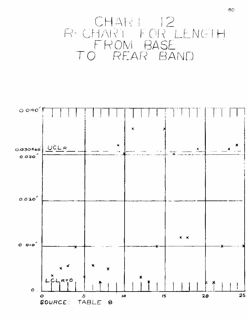
80

CHARI 1 1- CHAW ! I- OIC LL

FROM BASFT O REAR BAND

H

L1C L r0.030

0.0 2.0

O OIO

25203 15oSOURCE:: T A B L E 8

81

Table 9Measurements of Length from Base to Rear Band, Produced

by Trouble Free Machines(Values are expressed in units of 0 .001" in excess of3.400”. Dimension is specified as 3.48 + 0 .00” - 0.03 ")

Measurement Total R

67 66 67 64 64 328 368 69 70 77 76 360 962 62 64 62 71 321 972 70 70 78 77 367 875 71 70 64 66 346 1159 74 78 73 71 355 1975 73 77 68 79 372 1164 63 59 64 64 314 571 70 59 75 71 346 1672 68 66 72 67 345 679 66 67 55 69 336 2468 72 65 77 76 358 1275 75 71 63 62 346 1372 78 72 75 72 369 671 67 75 70 72 355 879 72 70 75 71 367 967 68 73 69 64 341 967 62 72 73 76 350 1475 73 72 73 75 368 367 68 71 75 78 359 1173 63 74 75 72 357 1268 71 77 71 71 358 963 62 78 78 70 351 1665 72 79 75 74 365 1464 61 72 72 75 344 14

Total

25

■ 70.224 10.84

UCL- - X ♦ A2R- 70.224 ♦ 0.5& x 10.84« 70.224 ♦ 6.287 » 76.511

LCL^ - X - A2R- 70.224 - 6.287- 63.937

8,778 271UCLr - D^R

■ 2.11 x 10.84 - 22.872

LCL - D R R 3" 0

CHART 13 x CHART FOR LENGTH FROM BASE TO REAR BAND PRODUCED BY TROUBLE FREE MACHINE

3 . ^ 0

3.+80

3 +76511

3.+702243 .470 "

3.4-43437

3.4-tO

3.4-50

3.4-40

UCL x

LCL*

10 IB 20s o u r c e :: t a b l e 9

32

25

CHART K

R-CHART FOR LENGTH FROM BASE TO REAR BAND

PRODUCED BY TROUBLE FREE MACHINE

0.030

UCl_ R

0.010

0.0(0

s 2.5o IO 2 0SOURCE: TABLE 9

84

Table 10Measurements of Length from Base to Rear Band,

after Improvement(Values are expressed in units of 0.001” in excess of 3.i+00”. Dimension is specified as 3*48" ♦ 0.00" - 0.03")

Measurement Total R80 79 75 64 45 343 3582 81 75 60 52 350 3079 79 77 58 44 337 3581 80 55 60 51 327 3080 75 79 68 60 362 2085 84 85 70 55 379 3084 59 67 80 52 342 3285 68 75 82 45 355 4080 72 73 68 60 353 2082 79 76 75 72 384 1079 52 75 77 49 332 3078 77 60 71 58 344 2080 55 57 60 55 307 2579 73 65 72 57 346 2280 67 55 78 51 331 2985 65 82 75 50 357 3580 78 80 55 45 338 3580 70 65 75 60 350 2079 69 67 53 49 317 3078 70 64 75 58 345 2079 59 75 60 54 327 2577 70 60 75 55 337 2275 63 52 75 51 316 2485 77 84 77 54 377 3180 65 59 70 55 329 25

Total1 - ^125^ " 66.680R - £15. - 27.000 25UCL— - X ♦ A R

A *v

- 68.680 ♦ 0.58 x 27 ** 68.680 ♦ 15*66- 64*34

LCL^ - X - A2R

8,585 675- 60.68 - 15.66- 53*02

UCLp « D R R 4■ 2.11 x 27.00- 56.97

l c l r - d3r

CHARI 15X-CHART FOR LENGTH

FROM BASE TO R F A R BANDAFTER AN

IMPROVEMENT

3.4-683.4-84-34*'

3.+80“

3.468660

3.4-65

3.4-53013.4-5©'

ii

3.4-4©

rrUCL. *

TTTT

.a.

LCL St

IT I I I

0 3 10SOURCE: TABLE 1C

JS ;o

CHART 16 R-CHART FOR LENGTH FROM BASE TO REAR BAND

AFTERIMPROVEMENT

0.0600.056*17

0.0 4-0

oozo

U C L R

I I I I I I I I

x- x

L C L R - O1

t t t t m

O 5 10s o u r c e : t a b l e : io

/6 ao 25

8?

Table 11Measurements of Diameter of Band Seat

(Values are expressed in units of 0.0001" in excess of 5.7850”. Dimension is specified as 5*60” ♦ 0.00” - 0.02” )

Measurement Total R

-47 21 39 -25 22 10 8617 -65 24 36 -44 -32 10187 63 55 46 -50 201 137

-26 105 34 69 76 253 13130 56 124 99 135 446 105

145 156 I69 123 139 732 46154 138 148 I63 149 752 25147 126 50 73 96 492 9793 72 158 96 147 566 8674 -56 -46 29 38 37 13292 -48 57 -49 63 115 141108 73 155 143 129 608 82

152 135 128 160 143 718 32137 128 146 132 112 655 3429 -43 -27 -32 -49 -122 78

-46 -27 -36 -29 11 -127 5793 144 137 128 115 617 51

139 128 146 155 149 717 27148 137 126 149 152 712 2648 37 -46 -29 -49 -39 97

145 -55 47 -42 -31 64 20097 64 75 112 135 483 7122 96 65 48 77 308 74-46 23 -37 -22 55 -27 10192 87 -49 -38 66 158 141

Total-yrjij “ 66.416

R - - 86.320UCLy - X ♦ AgR

- 66.416 ♦ 0.53 x 86.320- 66.416 ♦ 50.066 - 116.432

LCLy - X - A R■ 66.416 - 56*066

8,302 2,153- 16.350

U0Lr - DkR

- 2.11 x 86.32=* 182.135

LCL_ - D R

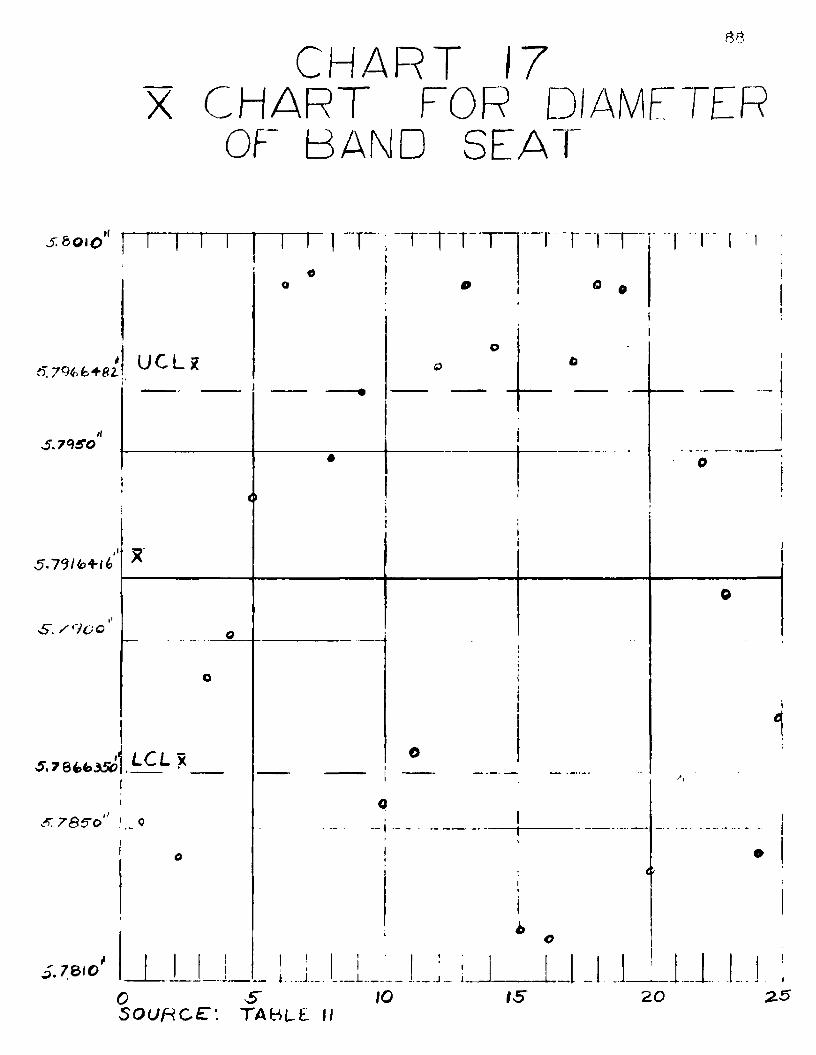
CHART 17 X CHART FOR DIAMFTFR

OF' BAND SEAT

* UCL 2

jj LC L x

/O_ .j _

s5"S O U R C E ' . TABLE.

200S O U R C E

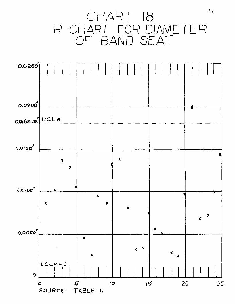
CHART 18 R-CHART FOR DIAMETER

OF BAND SEAT

>9

0.0 250

0.0100

0.018 2135

0.0150

0,0 too

0.0050

o

UCLR

LCLR =- 0

oSOURCE:

5“ 10TABLE II

15 20 25

90

Table 12Measurements of Diameter of Band Seat, Produced by

Trouble Free Machines(Values are expressed in units of 0.0001" in excess of 5.7750". Dimension is specified as 5*80" ♦ 0.00" - 0.02” )

Measurement Total R

187 169 148 149 180 833 39137 117 179 138 202 773 85113 170 170 178 187 818 74191 191 198 196 178 954 20130 158 205 131 170 794 75162 ii6 201 188 174 841 85152 188 183 I89 142 854 47188 151 165 165 139 808 49195 213 149 170 123 850 90176 170 129 169 162 806 47164 147 202 142 152 807 60118 159 198 159 169 803 80130 148 172 162 181 793 51187 162 178 177 199 903 37151 156 146 159 161 773 15203 120 141 146 132 742 83158 132 166 149 128 733 38177 188 I64 151 110 790 78206 161 133 181 130 811 76149 179 169 164 172 833 30199 169 193 172 158 891 41166 170 199 201 185 921 35158 178 132 143 133 744 46200 172 179 166 145 662 55158 103 148 180 158 747 77

Total 20,484 1,413Y „ „ i63 .e72 UCL^ , D^R a 2>11 x 56.52

R - * 4 ^ - 56.52 - 119.257UCLy - X ♦ ApR LCLp - 0

- 163.672 ♦ 0.56 x 56.52- 163.872 ♦ 32.782 « I96.654

LCL^ - 163.872 - 32.782- 131.090

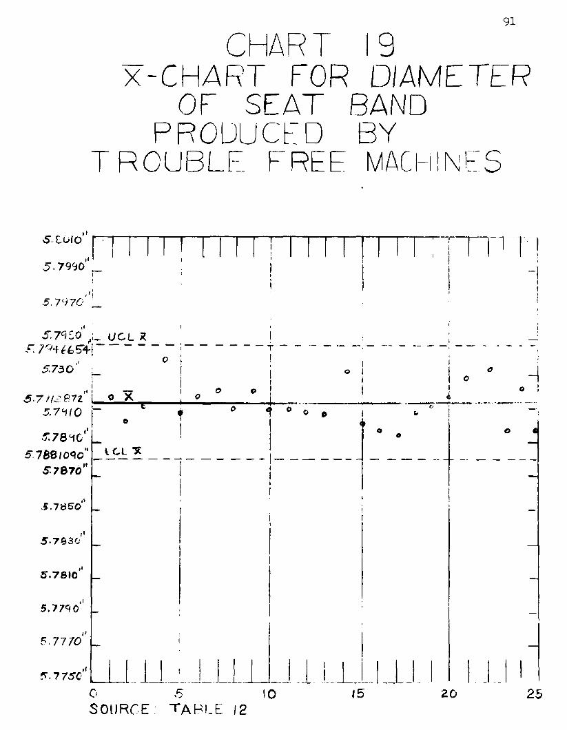
91

CHART 19 X-CHART FOR DIAMETER

OF SEAT BAND PRODUCED BY

TROUBLE FREE MACHINES

r5. 7990 _I''I5.7976 U

S7C>C0 UCL * S’. 7^465-+

5.730*5.7 m 97z" L 0 x

5.79/0

5789G' L5 788/090

5 7870

.5.7850 _

5.7Q30 _

5.7810 _

5.7790 _

5.7 7 70 _

5.7 75C _

1. I

0 ,5 10SOURCE: TABLE 12

CHART 2 0 R-CHART FOR DIAMETER

OF BAND SEAT PRODUCED BY

TROUBLE FREE MACHINES

0.0160'

0.0140

0-0120

0.0100

0 . 0 080

O.OOfeo

0.004-0

0.0020

M M M M I 1 1 1 l l I l M l " !

UCLK

XX

A XX >

* X )

X X * *x

XXA

. . . X

x X>

X

L C L f t - o

J J J !

)

! i I ! 1 1 1 iO 5"SOURCE*. T A B L E 12

10 15 20 25

Table 13Computation of Trial Control Limits for Control Chart for Per Cent

Defective in Diameter of Bourrelet

DateNumberInspected

nNumber of Defectives

FractionDefective

P3 4 . iifli-Si

f"nUCL

P ♦ 3 ^LCL

P - 3 ^

June 1 1049 7 C.0067 0.0114 0.0267 0.00392 949 6 C.OO63 0.0119 0.C272 0.00343 1000 4 0.0040 0.0116 0.0269 0.00376 1153 9 0.0076 0.0106 0.0261 0.00457 1105 0 c.cooo 0.0111 0.0264 0.00428 1091 18 0.0165 0.0111 0.0264 C.00429 1011 15 0.0148 0.0116 0.0269 0.0037

10 923 1 0.0011 0.0121 0.0274 0.003213 1032 13 0.0126 0.0115 0.0268 0.003814 1034 23 0.0222 0.0114 0.0267 0.003915 1252 13 C.0104 0.0104 0.0257 0,004916 957 31 0.0324 0.0119 0.0272 0.003417 1129 8 0.0071 0.0109 0.0262 0.004420 976 13 0.0133 0.0118 0.0271 0.003521 1050 22 C.0210 0.0114 0.0267 0.003922 1142 29 C.0254 0.0109 0.0262 0.004423 1334 47 0.0352 C.OlOl 0.0254 0.005224 1228 24 0.0195 0.0105 0.0258 0.004627 1295 34 0.0263 0.0102 0.0255 0.0051

Total 20712 317 e e • • • • • * • • • eF pdfc Q;Q153___ . ___3V P(l-P) «= 3 j/o.0153(1 - 0.0153) - 3 / 0.0153 * 0^9847

- 3 / 0T0I5O659I- 3 x 0.1227 » 0.3681

CHART 21P-CHART FOR DIAMETER

OF BOURRELET

PER CENTSCO

3.00

2.00

.00

-3 13-17 27D A T E : J U N E J 9 5 5 SOURCE : T A B L E 13

Table 14Computation of Trial Control Limits

Defective in Diameterfor Control Chart for of Recess Groove

Per Cent

DateNumberInspected

nNumber of Defectives

FractionDefective

P 3tf * 2— fp(l-p) UCLP ♦ 3 *

LCL P - 3fi

June 1 530 11 0.0206 0.0155 0.0298 0.00002 927 14 0.0151 0.0117 0.0260 0.00263 632 14 0.0166 0.0123 0.0266 0.00206 901 35 O.O366 0.0119 0.0262 0.00247 1103 16 0.0145 0.0107 0.0250 0.00366 1222 6 O.OO65 0.0102 0.0245 0.00419 1272 27 0.0212 0.0100 0.0243 0.0043

10 1271 6 0.0063 0.0100 0.0243 0.004313 1056 19 0.0160 0.0110 0.0253 O.OO3314 1452 27 0.0166 0.0094 0.0237 0.004915 1354 16 0.0116 0.0097 0.0240 0.004616 1419 19 0.0134 0.0095 0.0238 0.004817 1196 0 0.0000 C.01C3 0.0246 0.004020 1367 6 0.0059 0.0096 0.0239 0.004721 1300 30 0.0231 0.0099 0.0242 0.004422 690 16 0.0160 0.0119 C.0262 0.002423 1200 16 0.0150 0.01C3 0.0246 0.004024 1240 16 0.0129 0.0101 C.0244 0.004227 1101 6 0.0073 0.0107 0.0250 0.0036

Total 21635 310 * • • • e • • » « * * •

P - - 2^ § 5- - 0 > Q U 3____________________

3^P(1-P) - 3 >/(0.0143)(l - 0.0143) - 3 / o.Q143 x 0.9657- 3l/o.Ol409551 = 3 x 0.1167- O.356I

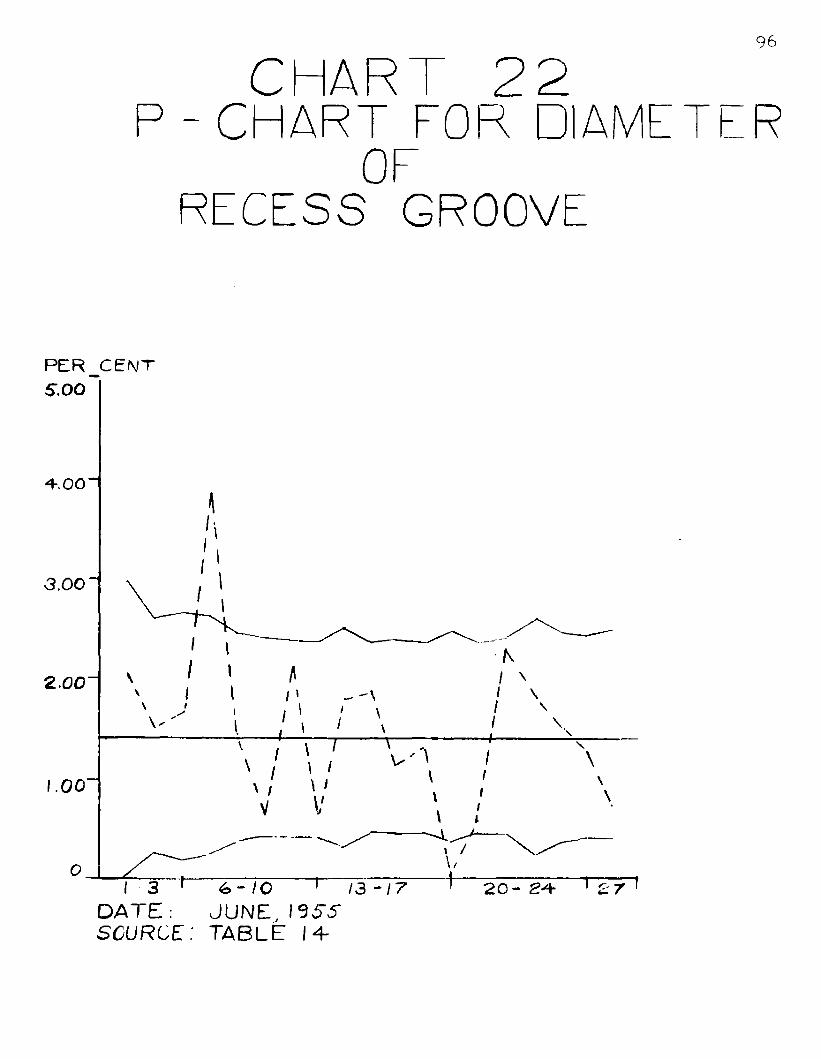
96

CHART 2 2 P - C H A R T FOR DIAMETEROFRECESS GROOVE

PER CENT5.00

3.00-

\.00~

D A T E : J U N E , I 3 5 SSOURCE: T A B L E 14-

Table 15Computation of Trial Control Limits for Control Chart for Per Cent Defective

in Length from Base to Rear Band

DateNumberInspected

nNumber of Defectives

FractionDefective

P3 ,

J m "UCL

P ♦ 3 *LCL

P - 3 ^June 1 530 24 0.0453 0.0150 0.0284 0.0000

2 927 9 0.0097 0.0113 0.0247 0.00213 832 7 0.0084 0.0120 0.0254 0.00146 901 14 0.0155 0.0115 0.0249 0.00197 1103 11 0.0100 0.0104 0.0238 0.00308 1222 15 0.0123 0.0099 0.0233 0.00359 1272 25 0.0197 0.0097 0.0231 0.0037

10 1271 20 0.0157 0.0097 0.0231 0.003713 1058 49 0.0463 0.0103 0.0237 0.003114 1452 36 0.0248 0.0090 0.0224 0.004415 1354 28 0.0207 0.0094 0.0228 0.004016 1419 0 0.0000 0.0092 0.0226 0.004217 1196 8 0.006? 0.0100 0.0234 0.003420 1367 14 0.0102 0.0093 0.0227 C.004121 1300 0 0.0000 0.0096 C.0230 0.003822 890 10 0.0112 0.0116 0.0250 0.001823 1200 5 0.0042 0.0100 0.0234 0.003424 1240 10 0.0081 0.0098 0.0232 0.003627 1101 5 0.0045 0.0104 0.0236 0.0030

TotalP - — 216

21635t0 » 0.0134 >35

290 * • * • e e * * • « • •

3 /PCI-P) - 3 V (0.0134) (1 - 0.0134) * 3 t/To.0134)(0.9866)=• 3 ? 0.01322044* 3 x 0.1150 = 0.3450

9?

CHART 2 3 P -CHART FOR

LENGTH hROM BAS _

TO REAR BAND

P E R C E N T5.00

4.CC ~

3.00 “

2.00 “

1.00

DATE: JUNE", 19 55S O U R C E : T A B L E 15

Table 16Computation of Trial Control Limits for Control Chart for Per Cent

Defective in Profile of Boat-Tail

DateNumberInspected

nNumber of Defectives

FractionDefective

P„ i&li-El

r r

UCL P ♦ 3 6

LCL P - 3 £

June 1 1049 36 0.0343 G.GI96 0.0667 0.02752 949 94 0.0991 c.0206 0.0677 0.02653 10C0 54 0.0540 0.0201 0.0672 0.02706 1153 67 0.0581 0*0187 0.0658 0.02847 1105 113 0.1023 0.0191 0.0662 0.02806 1091 61 0.0559 0.0192 0.0663 0.02799 1011 69 0.0682 0.0200 0.0671 0.0271

10 923 39 C.0423 0.0209 0.0680 ■ .026213 1032 43 0.0417 0.0198 0.0669 C.027314 1034 57 0.0551 0.0198 0.0669 0.027315 1252 20 C.0160 0.0180 G.0651 0.029116 957 25 0.0261 C.C205 0.0676 0.026617 1129 40 0.0354 0.0189 0.0660 0.028220 976 53 0.0542 0.0203 0.0674 0.026821 1050 26 0.0267 0.0196 O.C667 0.027522 1142 52 0.0455 C.0188 0.0659 0.028323 1334 59 0.0442 0.0174 0.0645 0.029724 1228 33 0.0269 c.0181 0.0652 0.029027 1295 33 0.0255 0.0177 0.0648 0.0294

Total976

20712

20712 = 0.0471

976

3 yp<i-p) - 3 0471)(1 - C.0471) 3^0.0471) (C.9529)3^0.0446̂ 159 3 x 0.21190.6357

100C H A R T 2 4-

P -CHART FORPROFI LE

OF BOAT-TAIL

PER CENT

.00 ~

-10.00

7.00~

3.0C-

2.0CT

1.00"

3- 17 T “' 20-2^-1-3 1 6'I0DATE: JUNE, IS55 27

S O U R C E : T A B L E 16

Table 17Computation of Trial Control Limits for Control Chart for Per Cent

Defective in Base Cover WeId

DateNumberInspected

nNumber of Defectives

FractionDefective

PJfea-p)

3 6 * r *UCL

P ♦ 3 6_LCL P - 34

June 1 530 24 0.0453 0.0154 0.0295 0.00002 927 27 0.0291 C.0116 0.0257 0.00253 632 67 0.0805 0.0123 0.0264 0.00186 901 8 0.0089 0.0113 0.0259 0.00237 1103 24 0.0218 0.0106 0.0247 0.00358 1222 18 C.0147 0.0101 0.0242 0.00409 1272 29 0.0228 0.GC99 0.0240 0.0042

10 1271 0 0.0000 0.0099 0.0240 0.004213 1058 12 0.0113 0.0109 0.0250 0.003214 1452 0 0.0000 0.0093 0.0234 0.004615 1354 7 0.0052 0.0096 0.0237 0.004516 1419 30 0.0211 0.0094 0.0235 0.004717 1196 0 0.0000 0.0102 0.0243 0.003920 1367 11 C .0080 0.0096 0.0237 0.004521 1300 24 0.0185 0.0098 0.0239 0.004322 69c 8 0.0090 0.0119 0.0260 0.002223 1200 6 0.0050 0.0102 0.0243 0.003924 1240 8 0.0065 0.0100 0.0241 0.004127 1101 3 0.002? 0.0106 0.0247 0.0035

Total 21635 306 • * • • • • • • • • • •306 0.014121635

rp(i-p) » 3 V(0.0141 )(i - 0.0141) 3 1/(0.0141)(0.9659) 3^.013901193 x 0.1179

102

CHART 2 5P-CHART

FOR BASE COVER WELD

8.05T %PER CENT S.00~\

4.00

3.00

2.00

1.00 _

27d a te : : JUNE:, /955- S O U R C E : T A B L E 17

CHAPTER VI SUMMARY AND CONCLUSIONS

Inherent variability is unavoidable. The recognition of the unavoidable inherent variability changes fundamentally the traditional concept of inspection. Applications of sta­tistical quality control are used to find if a stable pattern of variation exists, to learn when and where a change in the pattern of variation arises, and to tell when a process re­quires corrective actions.

Although the historical development of statistics is as old as that of mathematics, and although statistics has been applied to other fields for several centuries, the application of statistical methods to quality control is relatively new. Shewhart made the first sketch of statisti­cal control charts in 1924 and, in 1931, published Control of Quality of Manufacturing Product, which set the pattern for subsequent applications of statistical methods to process control.

During World War II, the armed services entered the market as large consumers. The armed services adopted sta­tistical sampling inspection procedures and brought direct pressure on producers of war products to adopt statistical

103

104

quality control methods in order to meet requirements of acceptance and to lower the rate of rejection of products.

The application of statistical quality control has been used in industries during the past two decades. The place of the statistical quality control group in the organisational structure of a company is, however, still a moot question. The importance of such control has been overlooked often by the top management, and even where it has been recognized, the merit of statistical quality control is often limited to the extent of technical consul­tation. These conditions result principally from an im­proper organizational structure.

The ideal type of organization for the small or medium-sized plant, as suggested in Chapter IV, is the authoritative pattern. Although this type of organization has not been used, the recommendation for its establishment is based on the theory pertaining to the assignment of authority and responsibility and on the suitable use of statistical quality control to the greatest possible extent.

A practical application of statistical quality control is introduced to Plant D. Plant D has not used methods of statistical quality control and statistical quality control methods have not been used in any plant of that kind.Plant D produces a kind of war material and deals exclusively

3 0.5

with governmental orders. The organizational structure of Plant D and the current manufacturing process are par­ticularized in Chapter III.

Plant D depends especially on inspection. Several hundred per cent repetitive inspections on continuous production have been practiced. The use of the repetitive inspection on continuous production is, however, subject to the psychological law of diminishing efficiency. The results of this plantfs policy are:

1. The cost of inspection becomes a great proportion of regular production cost;

i2. The cost of scrap increases rapidly and thereby output is decreased;

3* Rejections have not been so reduced to the minimum expected.

Statistical methods are used to solve these problems. The application provides the proper answers to the follow­ing questions:

1. Where are the most serious troubles?2. What are the assignable causes?3» How should they be corrected?

Statistical quality control applied for a short time reveals that Plant D does not have trouble in all i*l parts of the product. Major problems exist only in the following operations: the base thickness, the diameter of the recess

lof-

groove, the length from the base to the rear band, the diameter of the band seat, the diameter of bourrelet, the profile of boat-tail, and the base cover weld. These seven parts are the most important ones that cause numerous rejections and have high costs of rework or even high cost of spoilage.

Except the piercing operation which causes trouble in the base thickness, all other assignable causes are easily corrected, and hence the process can be easily brought into statistical control. If statistical quality control Is continuously applied in Plant D, the cost of inspection and the cost of scrap should decrease consider­ably and the occurrence of rejections should be reduced to a minimum. Such a result will yield Plant D a greater profit and the government a smaller coat paid for the product.

SELECTED RIBLIOGRAPHY

Books

Alford, L, P., and J. R. Bangs, Jr., editors. Production Handbook. New York: The Ronald Press Company, 194-4-.Pp. xv ♦ 1676.

Bowker, Albert H., and Henry P. Goode. Sampling Inspection by Variables. First Edition. New York: McGraw-HillBook Company, Inc., 1952. Pp. xi * 216.

Croxton, Frederick E., and Dulley J. Cowden. AppliedGeneral Statistics. Hew York: Prentice-Hall, Inc.,194-9. Pp. xviii ♦ 944.

David, F. N. A Statistical Primer. London: CharlesGriffin Company Limited, 1953* Pp. x ♦ 226.

Deming, W. E. Some Theory of Sampling. New York: John Wiley Sons, Inc., 1950. Pp. xvii + 602.

Dixon, Wilfrid J., and Frank J. Massey, Jr. Introduction to Statistical Analysis. Second Edition. New York: McGraw-Hill Book Company, Inc., 1957. Pp. xiii ♦ 4B&.

Dudley, John W,, Jr. Examination of Industrial Measure­ments. First Edition. New York: McGraw-Hill BookCompany, Inc., 1946. Pp. ix ♦ 113.

Duncan, Acheson J. Qua.1 J ty Control and Industrial Sta­tistics. Chicago: Richard D. Irwin, Inc., 1952.Pp. xxvii ♦ 663.

Elderton, William Palian. Frequency Curves and Correlation. Fourth Edition. Washington, D. C.: Harren Press,1953- Pp. xi ♦ 272.

Enrick, Norbert L. Quality Control. Second Enlarged Edition. New York: The Industrial Press, 1954.Pp. vlii ♦ 1B1.

107

10?

Feigrntaum, A. V. Qual1ty Control. Principles. Prac11ce. and Administration. First Edition. Mew York: McGraw-HIl 1 Rook Company, Inc., 1951. Pp. xi + 443*

Fisher, R. A., and F. Yates. Statistical Tables for Elological. Agricultural. and Medical Research. Edinburgh: Oliver and Boyd, Ltd., 1935. Table IV.

Freedman, Rudolph, and Joseph Movshin. A Basic Training ilanual on Statistical Qualitv Control. St. Louis, Missouri: St. Louis Society for Quality Control ,1959. P. 74.

Grant, Eugene L. Statistical Quality Control. SecondEdition. New York; McGraw-Hill Book Company, Inc., 1953. Pp. xvi ♦ 557.

Guide for duali t y Control and Control Chart Method of Analyzing Data. New YorV-: American StandardsAssociation Incorporated, 1941.

Hald, A. Stati3tical Tables and Formulas. New York;John V/iley and Sons, Inc., 1953* Pp. 40-45.

. Statls ti cal Theory with Engineering Applica­tions . New York: John V/iley and Sons, Inc., 1959.Pp. xi1 + 753.

Hanson, Permit (j . Managerial Statistics. Mew York: Prentice-Hall, Inc., 1955. Pp. xiv + 306.

Heide, John D. Industrial Process Control by Statistical Methods * First Edition. Mew York: McGraw-Hill Boo'-:Company, Inc., 1952. Pp. ix ♦ 297.

Juran, J. M. Management of Inspection and Quality Control. New York; Harper Brothers Publishers, 194^.Pp. xiv + 235.

. Editor. Quality Control Handbook. First Edition. Mew York; McGraw-Hill Book Company, Inc., 1951. Pp. viil ♦ 5CC.

Kennedy, Clifford V/. Qual 1 tv Control Methods. New York: Prentice-Hall, Inc., 1945. Pp. viii ♦ 243.

Peach, Paul. Industrial Statistics and Quality Control.Second Edition. Raleigh, M. C.: Edwards ■ BroughtonCo., 1947. Pp. xv ♦ 235.

109

Rutherford, John G. Quality Control in Industry. Methodsand Svaten.s . New YorV; Pitman Publishing Corporation, 19V*. Pp. xvii ♦ 201.

Cchrock, Edward M. puality Control and StatisticalMethods. New York: Reinhold Publishing Corporation,19r0. Pp. xi ♦ 213.

Chewhart, Walter A., and V7. Edwards Dend.nr. Statistical Method from the Viewpoint of Quality Control. Washington: The Graduate School, The Department ofAgriculture, 1939. Pp. ix ♦ 155-

Simon, Leslie E. An Engineers1 Ilanual of StatisticalMethods. New York; John Wiley £> Sons, Inc., 19A1.Pp. ix ♦ 231.

Tippett, L. H. C. Technological Applications of Statistics. New York’: John Wiley V Sons, Inc., 195G* Pp. ix ♦1*9.

Wharton, A. S. Quality Through Statistics. Second Edition. London: Philips Electrical Ltd., 197+6. Pp. iv ♦ M2.

Periodicals

"Applications of Statistical Method in Engineering andManufacturing," Mechanical Engineering. LIV(November, 1932), 77*-7*0.

Cassady, G. H., "Quality Control by Statistical Methods," Industrial Quality Control. II (January, 197+6), IE.

Dutton, H. P., "Quality Control," Factory Management and Maintenance. XCIII(1935)> 3-93-S-lC*.

Freeman, H. A., "Statistical Methods for Quality Control," Mechanical Engineering. LIX(April, 1937), 261-262.

Freeman, R. W. A., "Industrial Quality Control in the Foundry," Industrial Quality Control. II(January,197+6}, 11.

Goddess, Eugene, "Probability and Quality Control - II," American Machinist. XC(August, 19/+6), 116-119.

IK'

Olds, Edwin G., "Statistical Quality Control of Methodsand Materials," Metals and Alloys. XXII(October, 1945'), 1007-1101.

Pears.n, E. S., "The Percentage Limits for the Distribution of Range in Samples for a Normal Population,” Piometrika. XXIV(1932), 404-417.

. "The Probability Integral of the Range in Samples of N Observations from A Normal Population," Biometrika. XXXII(1941-1942), 3C1-30B.

Squires, Frank H,, "Changing Attitudes in Quality Control," Management Review. XLI{August, 1952), 506-309.

Thompson, Catherine X., "Table of Percentage Points of the Distribution," Biometrika. XXXII(1941-1942), 183-139.

Wilson, Edwin 3., and M. M* Hiferty, "The Distribution ofChi-square," National Academy of Science. Proceedings, XVII{1931), 0B4 ff.

Working, Holbrook, "Statistical Quality Control in WarProduction," American Statistical Association Journal. XL (December, 1945)',425-447.

VITA

ChuntI Wei Chen was i'orn in Hunan, China, on December 21, 1921 . In August, 1954, he received the decree cf I last or of business Administration from Louisiana State University.From September, 1954 on, he has pursued at the same Uni­versity further studies leading to the decree or Doctor of Philosophy.

111

EXAMINATION AND THESIS REPORT

Candidate: Chung V e i Chen

M ajor Field: Business A d m in istra tio n

Title of Thesis: Problems In the Application of Statistical Quality Controlto a Manufacturing PlantApproved:

M ajor Professor and Chairman

Dean ie Graduate School

EXAMINING COMMITTEE:

Date of Examination:

Mey 3, 1#7