problems in transport theorydspace.rri.res.in/bitstream/2289/4369/1/anupam kundu_thesis.pdf · this...
TRANSCRIPT

Problems in Transport theory
byAnupam Kundu
A Thesis submitted to theJawaharlal Nehru University
for the Degree ofDoctor of Philosophy
2010
Raman Research InstituteBangalore 560 080
India

Certificate:
This is to certify that the thesis entitled Problems in transport theory submitted by Mr.
Anupam Kundu for the award of the degree of Doctor of Philosophy of Jawaharlal Nehru
University is his original work. This has not been published or submitted to any other Uni-
versity for any other Degree or Diploma.
Prof. Ravi Subrahmanyan Prof. Abhishek Dhar
(Center Chairperson) (Thesis Supervisor)
Director, Raman Research Institute,
Raman Research Institute, Bangalore 560 080, INDIA.
Bangalore 560 080, INDIA.

Declaration:
I hereby declare that the work reported in this thesis is entirely original. This thesis is com-
posed independently by me at Raman Research Institute under the supervision of Prof. Ab-
hishek Dhar. I further declare that the subject matter presented in this thesis has not pre-
viously formed the basis for the award of any degree, diploma, membership, associateship,
fellowship or any other similar title of any university or institution.
(Prof. Abhishek Dhar) (Anupam Kundu)
Theoretical Physics,
Raman Research Institute,
Bangalore 560 080, INDIA.

Acknowledgement:
I would like to thank my supervisor Dr. Abhishek Dhar for his careful guidance throughout
my Ph.D. programme. He was always ready to help me in both academic and non-academic
matters. I have learnt a lot from him and most importantly how to be patient. He always has
encouraged me to think in new ways and gave me a lot of freedom. I would like to convey
my sincere regards and respect for his valuable involvement during the period of my graduate
research.
Recently, I have worked with Dr. Sanjib Sabhapandit. I had many great discussions with
him which helped me a lot in understanding many things in a better way. I enjoyed several
tea-time discussions with Dr. Joseph Samuel and Dr. Supurna Sinha. I wish to convey my
deep regards to them not only for academic discussions but also for non-academic advice.
It has been a very good stay at RRI doing my PhD work. Lots of people are responsible for
making this stay happening, interesting and enjoyable. I would like to acknowledge some
of my friends who have helped me in many aspects, namely, Suman, Arnab, Chandrakant,
Pragya, Suchana, Alok, Venkat. Apart from research and studies, I spent a lot of happy
hours with them. I would also like to thank all the football players of RRI for making many
evenings memorable.
I would like to thank my parents and Kalpana for their support and encouragement.
I wish to thank all the people in RRI, administrative as well as academic, for making this
stay enjoyable.
iii

PrefaceIn this thesis we study theoretical problems in transport phenomena. These phenomena
include the transport of heat or particles across a system due to the presence of external
driving forces such as temperature gradients or electric fields. Some well known laws re-
lated to these phenomena are Fourier’s law of heat conduction and Ohm’s law of electrical
conduction. These laws describe normal behaviour of macroscopic systems in nonequilib-
rium situations where external driving is weak and the system is close to equilibrium. There
have been many attempts to understand these laws from a microscopic approach in the same
spirit as one derives the thermodynamic properties of a system using equilibrium statistical
mechanics. Some of the well known theories that have been developed in this regard are
Boltzmann kinetic theory approach and the Green-Kubo formalism. However there are as-
sumptions that go into these approaches and these may not always be valid. Another more
recently developed theory is the non-equilibrium Green’s function (NEGF) method. In this
approach, which is closely related to the Landauer formalism, transport is viewed as a scatter-
ing problem in an open system which includes the reservoirs. In addition to these theoretical
approaches there have been many attempts to understand heat transport through direct simu-
lations of the microscopic equations of motion of the system with heat baths. These studies
suggest Fourier’s law is not valid in low dimensional systems and transport is anomalous.
Recent developments of nanophysics and mesoscopic physics have made it possible for the
experimental study of transport in low-dimensional systems and this provides further moti-
vations for microscopic theoretical analysis. The following problems have been addressed
in this thesis:
i) Is Fourier’s law valid in higher dimensional disordered harmonic systems? How does heat
current across such a system scale with system size in the asymptotic limit ? How does this
scaling law depend on boundary conditions?
ii) The applicability of the standard Green-Kubo formula to small systems and systems with
anomalous transport is problematic. We derive another linear response result for open classi-
cal systems which can be applied to both the above cases. We also obtain an exact analytical
iv

expression for the current-current time correlation function for harmonic chain.
iii) Another related problem studied in this thesis is on the properties of fluctuations of trans-
port current in various systems. An interesting result in this area, valid for systems far from
equilibrium, is the so-called fluctuation theorem. This theorem involves rare fluctuations of
the transport current whose probabilities are difficult to compute by usual simulations. In
this thesis we have developed an algorithm to find probabilities of vary rare events and ap-
plied it to non-equilibrium processes involving both heat and particle transport. We have also
calculated analytically the large-deviation function corresponding to the heat transfer across
a harmonic system.
The plan of the thesis is as follows:
Chapter (1) is an introduction to the thesis. Here in the first part we describe the transport
phenomena. Then we briefly discuss the methods and approaches applied to the theoretical
study of transport phenomena. We also discuss the problems and limitations associated with
these methods. Next part is devoted to some earlier studies relevant to our work. These are
theoretical studies as well as simulation studies on heat conduction, which provide motiva-
tions for our work.
In Chapter (2) we introduce the Langevin equation and Green’s function (LEGF) approach
to study heat conduction in harmonic systems. We discuss the approach for harmonic sys-
tems in detail because we extensively use this approach and ideas in our work. Briefly,
it involves solving a set of generalized Langevin equations by Fourier transforming them
and then finding expectation values of observables by taking an average over noise config-
urations. One finds that the current through the system in the non-equilibrium steady state
(NESS) can be written as an integral of a transmission function over all frequencies. The
final result is the same as obtained by the NEGF approach and has the form of the Landauer
formula. In the last section we discuss heat conduction in one-dimensional disordered har-
monic systems where there are some well established results. In the next chapter we extend
these ideas for one dimensional systems to understand heat conduction in higher dimensional
systems.
v

Chapter (3) reports extensive numerical studies on heat conduction in two and three di-
mensional disordered harmonic systems. In this chapter we investigate the asymptotic sys-
tem size dependence of the average heat current in the NESS. In the first section we use
heuristic arguments based on kinetic theory and localization theory to predict the size depen-
dence of the current for different boundary conditions. Next we calculate the current using
the Landauer-like formula discussed in chapter (2) and also through direct non-equilibrium
simulations. In our numerical approach we computed the transmission coefficient using an
efficient algorithm based on the recursive properties of the Green’s functions of the system.
We also study the nature of the phonon modes of the harmonic system without coupling to
heat baths. Finally we compare our numerical result against our heuristic predictions and
discuss them.
In the beginning of chapter (4) we discuss the Green-Kubo formalism to study systems
near equilibrium. We first briefly describe the existing mechanical derivation of the Green-
Kubo formula which gives the response of a system to small external perturbations. Then we
discuss the derivation of the corresponding formula for non-mechanical perturbations and the
limitations of the use of the formula in small systems and systems with anomalous transport.
Next we present our derivation of a similar linear-response formula for general open classical
systems. We also give a detailed calculation of the time auto-correlation function of current
for a disordered harmonic chain and show that it satisfies our open system formula. Unlike
the standard Green-Kubo formula, our linear response result for open systems is valid for
small systems and systems with anomalous transport.
Chapter (5) discusses a different problem in transport where we study properties of fluc-
tuations of the heat as well as particle current. In this chapter we analytically compute the
large deviation function of the probability distribution of heat transfer over a large time in-
terval across a harmonic chain connected to heat baths. The algorithm is applied to both heat
and particle transport. Next we describe an algorithm that we have developed to find the
probabilities of very rare events in transport process.
vi

Publications
• (1) Green-Kubo formula for open systems, Anupam Kundu, Abhishek Dhar, Onuttom
Narayan, J. Stat. Mech. (2009) L03001
• (2) Heat transport and phonon localization in disordered harmonic crystals, Anupam
Kundu, Abhishek Chaudhuri, Dibyendu Roy, Abhishek Dhar, Joel Lebowitz, Herbert
Spohn, EPL 90 (2010) 40001.
• (3) Heat transport and phonon localization in mass-disordered harmonic crystals, Ab-
hishek Chaudhuri, Anupam Kundu, Dibyendu Roy, Abhishek Dhar, Joel Lebowitz,
Herbert Spohn, PRB 81, (2010) 064301.
• (4) Time auto-correlation function and Green-kubo formula: A study on disordered
harmonic chain, Anupam Kundu, submitted to PRE.
• (5) Algorithm for finding probabilities of rare events and application to non-
equilibrium processes, Anupam Kundu, Sanjib Sabhapandit, Abhishek Dhar, Submit-
ted to PRL.
• (6) Large deviation of heat flow in harmonic chains, Anupam Kundu, Sanjib Sabha-
pandit, Abhishek Dhar, in preparation.
vii

Contents
1 Introduction 1
1.1 Various approaches in transport theory . . . . . . . . . . . . . . . . . . . . 2
1.1.1 Drude-Sommerfeld theory . . . . . . . . . . . . . . . . . . . . . . 2
1.1.2 Semiclassical Boltzmann kinetic theory: Boltzmann equation . . . 3
1.1.3 Green-Kubo linear response theory . . . . . . . . . . . . . . . . . 5
1.1.4 Non-equilibrium Green’s function formalism . . . . . . . . . . . . 8
1.2 Earlier studies on heat transport . . . . . . . . . . . . . . . . . . . . . . . 9
1.3 Problems addressed in the thesis . . . . . . . . . . . . . . . . . . . . . . . 16
2 Heat conduction in harmonic systems 18
2.1 Generalized Langevin equations and LEGF approach . . . . . . . . . . . . 19
2.2 Stationary solution of the equation of motion and steady state properties . . 24
2.3 Examples of baths . . . . . . . . . . . . . . . . . . . . . . . . . . . . . . . 31
2.4 Current in d-dimensional disordered harmonic lattice . . . . . . . . . . . . 34
2.4.1 Transfer matrix approach and recursion relations for Green’s functions 38
2.4.2 Current in one dimensional harmonic system: . . . . . . . . . . . . 41
2.4.3 Current in d-dimensional ordered harmonic system . . . . . . . . . 46
3 Study on heat conduction in higher dimensional harmonic system 48
3.1 Phonon localization . . . . . . . . . . . . . . . . . . . . . . . . . . . . . . 49
3.2 Kinetic theory . . . . . . . . . . . . . . . . . . . . . . . . . . . . . . . . . 51
3.3 System and methods . . . . . . . . . . . . . . . . . . . . . . . . . . . . . 51
viii

3.4 Heat conduction in disordered harmonic crystals: General considerations . 55
3.5 Results from Numerics and Simulations . . . . . . . . . . . . . . . . . . . 61
3.5.1 Results in two dimensions . . . . . . . . . . . . . . . . . . . . . . 61
3.5.1.1 Disordered 2D lattice without pinning . . . . . . . . . . 61
3.5.1.2 Disordered 2D lattice with pinning . . . . . . . . . . . . 70
3.5.2 Results in three dimensions . . . . . . . . . . . . . . . . . . . . . 74
3.5.2.1 Disordered 3D lattice without pinning . . . . . . . . . . 74
3.5.2.2 Disordered 3D lattice with pinning . . . . . . . . . . . . 81
3.6 Conclusions . . . . . . . . . . . . . . . . . . . . . . . . . . . . . . . . . . 85
3.7 appendix . . . . . . . . . . . . . . . . . . . . . . . . . . . . . . . . . . . . 87
4 Green-Kubo formula for open systems 88
4.1 Proof of the formula for 1D lattice model . . . . . . . . . . . . . . . . . . 90
4.2 One dimensional lattice with other baths . . . . . . . . . . . . . . . . . . . 95
4.3 Lattice models in higher dimensions . . . . . . . . . . . . . . . . . . . . . 97
4.4 Fluid system coupled to Maxwell baths . . . . . . . . . . . . . . . . . . . 99
4.5 Proof of the formula for boundary currents . . . . . . . . . . . . . . . . . . 102
4.5.1 Definition of the model . . . . . . . . . . . . . . . . . . . . . . . 102
4.5.2 Steady state properties and current calculation . . . . . . . . . . . 104
4.5.3 Calculation of auto-correlation function . . . . . . . . . . . . . . . 106
4.5.4 Numerical results . . . . . . . . . . . . . . . . . . . . . . . . . . . 108
4.6 Conclusions . . . . . . . . . . . . . . . . . . . . . . . . . . . . . . . . . . 113
4.7 appendix . . . . . . . . . . . . . . . . . . . . . . . . . . . . . . . . . . . . 114
4.7.1 Proof of Eq. [4.55] . . . . . . . . . . . . . . . . . . . . . . . . . . 114
4.7.2 Expressions of K1s . . . . . . . . . . . . . . . . . . . . . . . . . . 115
5 Large deviations in transport processes 116
5.1 Large deviation function of heat flow in harmonic chain . . . . . . . . . . . 117
5.1.1 Derivation . . . . . . . . . . . . . . . . . . . . . . . . . . . . . . . 122
ix
5.1.2 Single Brownian particle . . . . . . . . . . . . . . . . . . . . . . . 129
5.2 Algorithm for finding probabilities of rare events . . . . . . . . . . . . . . 131
5.2.1 The algorithm . . . . . . . . . . . . . . . . . . . . . . . . . . . . . 132
5.2.2 Symmetric simple exclusion process . . . . . . . . . . . . . . . . . 133
5.2.3 Heat conduction . . . . . . . . . . . . . . . . . . . . . . . . . . . 135
5.3 Conclusions . . . . . . . . . . . . . . . . . . . . . . . . . . . . . . . . . . 139
5.4 Appendix . . . . . . . . . . . . . . . . . . . . . . . . . . . . . . . . . . . 139
5.4.1 Expression of the matrix E(ω) : . . . . . . . . . . . . . . . . . . . 139
5.4.2 Expressions of the elements of J(λ, ω) and c(ω) : . . . . . . . . . . 141
x
1 Introduction
We know that when an external electric field is applied across a conductor, an electrical
current flows across the system. Similarly when a chemical potential difference or a temper-
ature difference is maintained across a system, then particle current or energy current flows
through the system. These are examples of transport phenomena. Normally these phenom-
ena are described by phenomenological laws, namely Ohm’s law of electrical transport and
Fourier’s law of thermal transport. For electrical conduction, the current density je through
the system is proportional to the applied electrical field E:
je = σE (1.1)
and for thermal conduction, the heat current density jth is proportional to the temperature
gradient ∇T :
jth = −κ∇T. (1.2)
The proportionality constants σ and κ are called electrical conductivity and thermal conduc-
tivity respectively. These proportionality constants are normally known as transport coeffi-
cients. These characterise the transport properties of a macroscopic substance. One of the
main interest in the theoretical study of transport phenomena is to understand these laws and
compute the transport coefficients from a microscopic point of view. Attempts to derive these
laws starting from microscopic description of a system, have been started long back. All
these attempts have led to various theoretical techniques. Clearly these are non-equilibrium
phenomena and their study also has provided new understanding in non-equilibrium physics.
In sec. (1.1) of this chapter we will briefly discuss the different approaches used to understand
1

charge and energy transport. In Sec. (1.2) we discuss the earlier results in heat conduction.
Finally, in Sec. (1.3) we describe the problems addressed in this thesis.
1.1 Various approaches in transport theory
One of the main goals of a complete theory of transport would be to derive linear response
formulae such as Eqs. (1.1,1.2) starting from a microscopic description in the usual frame-
work of statistical mechanics. This task seems to be very difficult. The earliest attempts
were aimed at finding heat conductivity of gases using kinetic theory. Later Drude applied
kinetic theory to gas of conducting electrons in metal to study transport phenomena. In case
of thermal conduction in insulating solids Debye applied kinetic theory to gas of phonons.
In 1929 R. Peierls formulated Boltzmann equation for phonons to study thermal transport in
solids. Since then Peierls-Boltzmann theory became a cornerstone in the theory of thermal
conduction in solids. Later several other theoretical approaches were developed to study
transport and these include Green-Kubo formalism, Landauer formalism, non-equilibrium
Green function formalism etc. In the following we will discuss these approaches.
1.1.1 Drude-Sommerfeld theory
In 1900 Drude made one of the first attempt to derive these phenomenological laws Eq. (1.1)
and (1.2) of charge and energy conduction by conducting electrons in metals, starting from a
microscopic point of view . He applied kinetic theory of gas to conducting electrons moving
in the field of heavy ions which form the underlying lattice. In spite of electron-electron in-
teraction and electron-ion interaction Drude model treats this metallic gas as a neutral dilute
gas in which kinetic theory can be applied. The basic assumptions in this theory are [1]: (i)
Between successive collisions and in the absence of electromagnetic field the electrons move
uniformly in a straight line. (ii) The effect of interactions are taken into account by simply
considering that electrons suffer random collisions. As in kinetic theory the collisions are
modeled as instantaneous events which alter velocities abruptly. The probability of an elec-
tron undergoing a collision in time dt is dt/τ where τ is a phenomenological parameter and
2
known as relaxation time. (iii) Electrons are assumed to achieve thermal equilibrium with
their surroundings only through collisions.
Though the Drude model neglects the details of both the electron-electron and electron-
ion interactions, it was quite successful to explain Ohmic behaviour of metallic conductor,
Fourier’s law of thermal conduction (assuming local thermal equilibrium achieved by colli-
sions) and phenomenological Wiedemann-Franz law. From Drude model one gets explicit
forms of the transport coefficients σ and κ in terms of the electron density n, charge e, mass
m, mean velocity v and a single phenomenological parameter τ. The expressions for σ and κ
are following
σ =ne2τ
m, (1.3)
κ =13
v2τCV , (1.4)
where CV is the electronic specific heat. We note that the thermal conductivity can also be
expressed in terms of mean free path ` = vτ as :
κ =13
v`CV . (1.5)
The ratio κ/σT = 3K2B/2e2 gives the Lorentz number. Here KB represents Boltzmann con-
stant. The agreement of this number with experimental results was one of the success of
Drude theory. A more correct approach is to use the Fermi-Dirac distribution for the elec-
trons velocities. Using Fermi-Dirac distribution, Sommerfeld obtained a more correct ex-
pression for the Lorentz number: κ/σT = π2K2B/3e2.
1.1.2 Semiclassical Boltzmann kinetic theory: Boltzmann equation
In kinetic theory picture, one considers a gas of interacting particles which are the carriers
of heat or charge. The usual carriers are molecules of a gas, electrons in a metal, phonons
in crystalline solid etc. These carriers experience random collisions and Kinetic theory gives
an expression for the conductivity in terms of the mean free path `.
The Boltzmann equation approach is a more systematic way of deriving kinetic theory re-
3

sults. Let us first discuss this for electrons in metals. In this approach one considers electrons
at time t labelled by mean position r and mean momentum k. Between successive collisions
electrons are described by a wave packet. One then defines a non-equilibrium distribution
function g(r,k, t) such that, g(r,k, t)drdk/4π3 is the number of electrons at time t in the
semiclassical phase space volume drdk about the point r, k. It is assumed that between
two successive collisions, r and k evolve according to the semiclassical equations of motion
under the influence of external forces [1, 2, 3].
The time evolution equation of the distribution function g(r,k, t) is given by the Boltzmann
equation:
∂g∂t+ v.∇r g + F.
1~∇k g = (
∂g∂t
)coll
where, v =1~∇k E(k), (1.6)
and E(k) is the energy dispersion for electrons. In the above equation F represents the ex-
ternal forces and (∂g/∂t)coll represents the contribution from collisions. The collision term
in the right hand side of the above equation is calculated using different approximations in
different situations. Very often it is calculated using Fermi golden rule. The final result is
quite often in the form of the kinetic theory answers κ ∼∫
dkckvk`k, with an explicit form
for the mean free path `k. In high temperature regime the main source of collision in metal is
the lattice thermal vibrations, whereas impurities are the source of scattering in low temper-
atures. Surface or boundary scattering are dominant source of scattering in nanostructures
like quantum wires, quantum tubes, dots etc. Next we discuss the case of heat conduction in
crystalline solids.
In crystalline solids, the dynamical entities are the ions which are arranged (mean po-
sitions) in a regular periodic array forming the lattice. At non zero temperature this ions
oscillate about their mean positions. The normal modes of the lattice vibrations are called
phonons, which are the carriers of heat in metals as well as in electronic insulators. Debye,
like Drude, treated this vibrating lattice as a gas of phonons and applied kinetic theory to
express the phonon thermal conductivity κph in terms of the phonon specific heat per unit vol-
4
ume cphV , mean velocity v and mean free path ` as κph ∼ cph
V v`. Later Peierls wrote Boltzmann
equation for phonons [4] and showed how important anharmonicity, and specifically Ump-
klapp precesses, is in giving rise to finite lattice thermal conductivity. Solving the Boltzmann
equation in the relaxation time approximation gives a simple kinetic theory like expression
for the thermal conductivity, κph ∼∫
dkckv2kτk, where τk is the time between collisions, and
k refers to different phonon modes of the crystal. The relaxation time τk can get contributions
from various sources. In case of phonon conduction the main source of scatterings are impu-
rities and phonon-phonon interactions. Impurity scattering can arise due to the randomness
of the masses of the ions and force constants, whereas the phonon-phonon scattering arises
due to the higher order terms (beyond quadratic order) in the expansion of inter-particle po-
tential. In three dimensional solids, the Peierls-Boltzmann theory is well-developed [2, 3, 4]
and probably quite accurate. Only problem with Peierls-Boltzmann theory is that meaning
of g(r,k, t) is not very clear since phonons are extended objects. The recent work of Spohn
and Lukkarinen [5, 6] tries to give a rigorous basis for the phonon Boltzmann equation.
1.1.3 Green-Kubo linear response theory
Earlier two approaches of transport considers classical or semiclassical motion of interacting
carriers with appropriately introduced incoherent scattering mechanisms. Now we discuss a
general theory of transport called the Green-Kubo formalism which can be applied to both
classical and quantum systems. In this formalism one prepares a system in equilibrium and
then applies a small perturbation to the system. Due to this small perturbation the system
will be slightly out of equilibrium. In response to the perturbation, the expectation val-
ues of observables will change from their equilibrium values. In this formalism one finds
this response to linear order in perturbation strength. One finally obtains a formula which
provides a relation between the transport coefficients, such as electrical conductivity or the
thermal conductivity, and appropriate equilibrium time correlation functions. This formula
has been proved both for mechanical perturbations (perturbations in Hamiltonian) and non-
mechanical perturbation (perturbation in the boundary condition). Here we briefly sketch the
5

derivation of this formula for mechanical perturbation.
Let us consider a quantum system in thermodynamic equilibrium which is described by
a time-independent Hamiltonian H0 and temperature T (inverse temperature is β = 1/KBT
where KB is the Boltzmann constant). We assume that in the long past t = −∞ the perturba-
tion is switched on. Now the total Hamiltonian is
Htot = H0 + Hp where Hp = f (t)B. (1.7)
In the above expression f (t) represents the strength of the perturbation, for example electric
field, magnetic field etc. At t = −∞ the expectation value of any operator A is given by
〈A〉0 = trρ0A, (1.8)
where, ρ0 is the equilibrium density matrix. Because of the perturbation the steady state
expectation value of A will change. The change is given as
δ〈A(t)〉 = trδρ(t)A, where, δρ(t) = ρ(t) − ρ0. (1.9)
We find δρ(t) from the time evolution equation of ρ(t)
i~∂ρ
∂t+ [ρ, Htot] = 0 with ρ(−∞) = ρ0, (1.10)
where, [..] represents commutation operation. Since we want δρ(t) to be linear order in f ,
we expand above expression and keep terms linear order in f . In the interaction picture
(AI(t) = eiH0tAe−iH0t) we get
i~∂δρI
∂t= −[ρ0, HI
p] with δρI(−∞) = 0, (1.11)
whose formal solution is
δρI(t) =i~
∫ t
−∞
dt′[ρ0, HIp(t′)]
=i~
∫ t
−∞
dt′ρ0
∫ β
0dλ[HI
p(t′ − iλ~), H0]
6
= −
∫ t
−∞
dt′ρ0
∫ β
0dλ ˆHI
p(t′ − iλ~). (1.12)
In the second line of the above equation we have used the following relation:
F(β) = [V I(t′), e−βH0] = −e−βH0
∫ β
0dλ[V I(t′ − iλ~), H0], (1.13)
and in the third line we have used the time evolution equation of operators in the interaction
picture. Using the above solution given in Eq. (1.12) we calculate δ〈A(t)〉 and get
δ〈A(t)〉 = −∫ t
−∞
dt′ f (t′)∫ β
0dλtrρ0
ˆBI(t′ − iλ~)AI(t)
= −
∫ t
−∞
dt′ f (t′)∫ β
0dλ〈 ˆBI(t′ − iλ~)AI(t)〉0
=
∫ ∞
−∞
χAB(t − t′) f (t′). (1.14)
where,
χAB(t − t′) =∫ β
0dλ〈 ˆBI(t′ − iλ~)AI(t)〉0Θ(t − t′) (1.15)
Thus the response χAB(t−t′) = δ〈A(t)〉/δ f (t′) is related to the equilibrium correlation function
CAB(t − t′) = 〈 ˆBI(t′ − iλ~)AI(t)〉0. In the classical limit ~ → 0 which is equivalent to β → 0
we may approximate the formula in the second line of Eq. (1.14) as
δ〈A(t)〉 = −β∫ t
−∞
dt′ f (t′)〈 ˆB(t′)A(t)〉0. (1.16)
The results in Eqs. (1.15,1.14) are referred to as the Green-Kubo formula.
Now let us consider the case of electrical conduction in a gas of N electrons contained
in a one dimensional box of length L. Let xl be the position of the lth particle and e be the
charge of electron. The density of electrons at x is given by: n(x) =∑
l δ(x − xl). Now we
perturb the system by applying an electrostatic potential φ(x, t). The perturbation is written
as Hp = e∫ L
0eεtφ(x, t)n(x, t) where ε is a positive parameter which controls the rate at which
the field is switched on. From continuity equation ˆn(x, t) = −∂ j(x, t)/∂x, one defines the
7

electrical current as j(x, t) =∑
l xlδ(x− xl). If we take A = j(x, t) then from Eq. (1.16) we get
〈 j(x, t)〉 = −e∫ t
−∞
dt′∫ L
0dx′eεt
′
φ(x′, t′)〈 ˆn(x′, t′) j(x, t)〉0. (1.17)
Using continuity equation and doing a partial integration one gets
〈 j(x, t)〉 = βe∫ t
−∞
dt′eεt′
∫ L
0dx′E(x′)〈 j(x, t) j(x′, t′)〉. (1.18)
where we have ignored boundary terms requiring that currents at the boundaries are zero.
One can show that only in the limit L → ∞ then ε → 0, 〈 j(x, t)〉 , 0 [7]. For constant
electric field one defines the electrical conductivity as σ = 〈 j(x, t)〉/E and is given by
σ = βe limε→0
∫ ∞
0dte−εt lim
L→∞
∫ L
0dx′〈 j(x, t) j(x′, 0)〉. (1.19)
In terms of total current J =∫ L
0dx j(x) the above formula reads as
σ = βe limε→0
∫ ∞
0dte−εt lim
L→∞
1L〈J(t)J(0)〉. (1.20)
This is the Green-Kubo formula (GK) for electrical conductivity. As shown by Luttinger [7]
one can do a mechanical derivation for thermal conduction and this gives a similar formula
for thermal conductivity which looks like
κ =1
KBT 2 limε→0
∫ ∞
0dte−εt lim
L→∞
1L〈JE(t)JE(0)〉, (1.21)
where JE is the total energy current.
1.1.4 Non-equilibrium Green’s function formalism
The Non-equilibrium Green’s function formalism (NEGF) is a highly developed technique.
It was first invented in the context of quantum transport to calculate the steady state prop-
erties of a finite system connected to reservoirs [8, 9]. The reservoirs are modeled by non-
interacting Hamiltonians with infinite degrees of freedom.
As an example consider a system of electrons, which is in contact with reservoirs which are
themselves gas of non-interacting electrons. One starts with the system initially decoupled
8
with the reservoirs, which are in equilibrium at different temperatures and different chemical
potentials. The initial state of the system and the decoupled reservoirs are described by a
well defined density matrix. Considering that at t = −∞ the couplings of the system with the
reservoirs are switched on, one evolves the density matrix with this full Hamiltonian given
by
H = Hs + HL + HR + VLs + VRs (1.22)
where Hs is the system Hamiltonian, HL,R are Hamiltonians of left and right reservoirs and
VLs, VRs are couplings of the system with the left and right reservoirs. Now the density
matrix of the entire system (system plus reservoir) is evolved for an infinite time so that
one eventually reaches a non-equilibrium steady state (NESS). Various physical observables
such as currents, densities, etc, can be calculated using this non-equilibrium density matrix.
For non-interacting systems one obtains an expression for the steady state current in terms of
transmission coefficient of the carriers across the system. These expressions are basically the
same expressions that one obtains from the Landauer formalism [10] where, one thinks of the
transport through the system as a quantum mechanical scattering process. For noninteract-
ing systems, an equivalent and simpler approach is Langevin equation and Green’s function
approach (LEGF), where instead of the density matrix one deals with the Heisenberg equa-
tions of motion for the dynamical variables. Integrating out the bath degrees of freedom
one obtains a Generalised Langevin equation. For classical system the two approaches are
like considering the Fokker-Planck approach versus the Langevin approach. It is possible to
show that one can get all the results of NEGF, from LEGF approach. We discuss the LEGF
approach in chapter (2) in detail.
1.2 Earlier studies on heat transport
As discussed in the beginning of sec. (1.1), one of the goals in the theoretical study of heat
transport is to derive Fourier’s law from a statistical mechanical calculation. But this task is
formidably difficult. As is usual in theoretical physics, the guiding criterion of mathematical
9

simplicity leads one naturally to consider simple mathematical models which are able to
provide more detailed understanding to the necessary and sufficient conditions needed to
prove Fourier’s law.
One of the commonly used tests of Fourier’s law is to look at the dependence of heat current
density on the system size. Let j be the heat current density flowing through the system in
the steady state due to the small temperature difference ∆T applied across a system of linear
size N. Now let us define the finite system conductivity as
κN =jN∆T
. (1.23)
Then the conductivity appearing in Fourier’s law is given by
κ = limN→∞
lim∆T→0
κN . (1.24)
The validity of Fourier’s law requires the above limit to be finite and in that case Eq. (1.23)
and (1.24) imply that j should scale as N−1 in the large N limit (asymptotic limit). But in
many cases, especially in low dimensional systems, it is seen that
j ∼ N−µ, (1.25)
with µ , 1. The thermal conductivity behaves then as κN ∼ Nα where α = 1 − µ. For two
dimensional systems there are some analytic studies which suggest κ ∼ ln(N). Fourier’s law
holds only if α = 0. Some important questions are to find the scaling exponent α and to
decide the necessary and sufficient conditions for the validity of Fourier’s law. Below we
give a summery of earlier studies addressing these questions. From now onwards κN will be
denoted by κ only.
The harmonic crystal is a good starting point for understanding heat transport in solids. In
the non-equilibrium case, the problem of heat conduction in a classical ordered 1D harmonic
crystal was studied for the first time by Rieder, Lebowitz and Leib (RLL)[11]. Considering
the case of stochastic Markovian baths they were able to obtain full phase-space probability
distribution in the steady state exactly. Using this distribution they showed that temperature
10

in the bulk of the system is equal to the mean value of the two bath temperatures and ob-
tained an expression for the steady state current and also showed that in the large system size
limit current is independent of system size. Nakazawa (NK) [12] obtained the exact non-
equilibrium steady state distribution for an ordered harmonic chain with an onsite harmonic
potential at all sites and extended these results in higher dimensions. Results of RLL and
NK papers were also obtained by Dhar and Roy [13] using LEGF approach. The conclusion
that one draws from these studies is, the heat current in an ordered harmonic lattice is inde-
pendent of system size κ ∼ N (for large systems). This result is expected since there is no
mechanism for scattering of heat carriers, namely the phonons, and hence transport is ballis-
tic. One then thinks of introducing scattering mechanism to get Fourier’s behavior. There are
two ways of introducing scattering of phonons (i) introduction of disorder in the system (ii)
introduction of anharmonicity which would cause phonon-phonon scattering. Disorder can
be introduced in various ways, for example by making the masses of the particles random
or by making the spring constants random. Anharmonicity can be introduced by making the
interaction force anomg the particles non-linear. First we state earlier results on disordered
harmonic systems and next we will give results in interacting (anharmonic) systems.
Disordered harmonic systems: In this case the carriers of heat are the normal modes of
lattice vibrations (phonons). Since the normal modes take part in the conduction of heat it
is expected that heat conduction in disordered harmonic systems will be strongly affected
by the physics of Anderson localization. This was first discovered in disordered electronic
systems. Because of multiple scattering electronic states become localized at some point
in space, where it’s amplitude is significant and it decays exponentially from that point. In
fig. (1.1) we show typical examples of extended and localized states, where ξ represents the
localization length.
One can thus expect the same kind of physics as in electronic systems where localization was
first studied. In fact the problem of finding the normal modes of the disordered harmonic
lattice can be directly mapped to that of finding the eigenstates of an electron in a disordered
potential and described by the tight binding model (see chapter (3)). The effect of localization
11

0 200 400 600 800 10000
0.001
0.002
0.003
0.004
0.005
0 200 400 600 800 10000
0.005
0.01
0.015
0.02
0.025 ξ
Extended state
Localized state
Figure 1.1: Typical plots of an extended state and a localized state with localization length ξ.
on transport in phonon case is much the same as in electron case except for the following two
facts : (a) In the absence of external potential, the translational symmetry of the system leads
to the fact that low frequency modes are not localized and hence contribute to transport.
(b) Secondly, in the phonon case all frequencies participate in transport whereas electron-
transport is dominated by electrons near Fermi level. Because of these two differences, the
disordered harmonic crystal in one and two dimensions is not a heat insulator in contrast to
the electron case.
One of the earlier important work on phonon heat transport in disordered systems was
by Matsuda and Ishii (MI) [14] who showed that all high frequency modes in a disordered
harmonic chain were exponentially localized and this led to anomalous transport. They
also showed that, for small ω the localization length in an infinite chain goes as ω−2. This
implies that, localization length for normal modes with frequency ω < N−1/2 is greater than
N and these low frequency modes are extended and hence they participate in transport. The
disordered harmonic chain has been extensively studied by several authors [15, 16, 17, 18,
12
19, 20, 21, 22]. Two different models of baths and boundary conditions have been studied:
(i)white noise bath (WNB) (ii) Rubin’s model of baths (R). In the second model, baths are
itself modeled as semi-infinite ordered harmonic chains. One of the main conclusions was
that the exponent α depends on the choice of boundary conditions (BCs). For free BC ( no
external forces acting on the system ) one gets α = 1/2 while for fixed BC ( external forces
acting at the boundaries only) one gets α = −1/2. Another model was studied by Bolsteri
et al. [23], in which they have connected each site of a harmonic chain to a self-consistent
reservoirs to introduce scattering of phonons. Bonetto et al.solved this model exactly and
proved the existance of local thermal equilibrium and the validity of Fouriers law. Later this
model model was again studied by Dhar and Roy [24] using LEGF approach in both the
classical and quantum cases.
There are very few studies on the problem of heat conduction in higher dimensional dis-
ordered systems. These include study of localization properties in disordered continuous
elastic media by John et al. [25] using renormalization group theory, simulation studies on
two-dimensional harmonic system with bond-missing disorder by Lei yang [26] and simu-
lation studies on harmonic crystal in 2D with binary mass disorder by Lee and Dhar [27].
In their study John et al. showed that : in one dimension, all modes with ω > 1/N1/2 are
localized; in two dimensions, all modes with ω > 1/[log(N)]1/2 are localized and in three
dimensions, there is a finite band of frequencies of non-localized states. However, this study
was unable to extract the system size dependence of heat current in a disordered lattice in
any dimension. By simulating the Langevin equations for two different heat bath models
Lee and Dhar obtained different system size dependence of the conductivity. With fixed BCs
they obtained α ≈ 0.41 for white noise baths and for exponentially correlated Gaussian noise
bath it is 0.49.
Interacting systems: The other way of introducing scattering of phonons is to include an-
harmonicity in the system. There are few analytic results for one dimensional interacting sys-
tems and all of them are based on the use of Green Kubo formula. Mainly three different ap-
proaches have been used to study interacting systems which are: renormalization group (RG)
13

theory of hydrodynamic equations, mode coupling theory (MCT) and the Peierls-Boltzmann
kinetic theory approach. All these theories aim at calculating the equilibrium current-current
time auto-correlation C(t) = 〈 j(t) j(0)〉.
Narayan and Ramaswamy [28] introduced the first approach in the study of transport phe-
nomena and used RG theory to study transport phenomena in a one dimensional system of
interacting particles described by the following density fields: number, momentum and en-
ergy densities respectively, corresponding to the following conserved quantities: total num-
ber of particles, total momentum and total energy respectively. Using RG they obtained that
C(t) ∼ t−2/3 for large t and putting a upper cut-off tN ∼ N in the GK formula they obtained
α = 1/3.
The MCT approach was first introduced by Lepri, Livi and Politi [29] in the study of
energy conduction and has subsequently been used by several other authors [29, 30, 31, 32,
33]. In this theory one tries to calculate the slow relaxation of spontaneous fluctuations
of long-wave length modes since in low dimensional systems it is related to the long time
tails of C(t). Inserting this C(t) into the GK formula (with a cutoff ∝ N) one obtains the
value of α. Predictions are different for different situations. When the anharmonic potential
carries a cubic leading power then α = 1/3 whereas for a quartic leading order α = 1/2.
There are many computer simulation attempts on energy transport in FPU chains and other
interacting models to sort this disagreement, but different simulations gave various exponents
[29, 34, 32, 35, 36, 37, 38]. People have studied joint effects of anharmonicity and disorder
on the system size dependence of heat current in FPU chains [39]. Simulation in disordered
anharmonic chains by Dhar and Saito [40] found that the asymptotic power law dependence
of current on system size always dominated by anharmonicity and got α = 1/3.
There are studies in fluid systems with non-linear interactions. A number of studies were
made for momentum conserving (translationally invariant) systems using non-equilibrium
simulations and using the GK formalism [41, 42, 43, 44, 45, 46, 47]. The values of α obtained
in these studies do not match. In momentum non-conserving systems, in addition to interpar-
ticle interaction, particles experience external potentials. All studies in these kind of model
14
systems agree upon Fourier like behaviour in large system size limit [41, 48, 49, 50, 51, 52].
Effects of interaction have been studied in higher dimensional systems both theoretically and
numerically. The MCT and hydrodynamic approach predict that for momentum conserving
systems, the thermal conductivity diverges logarithmically in two dimensions and finite in
three dimension. But reported values of α in various numerical studies in two dimension do
not agree [53, 54, 55, 56]. In the presence of pinning all theories predict a finite conductivity
in all dimensions. In a very recent simulation, Saito and Dhar [57] provided first verifica-
tion of Fourier’s law in a 3D anharmonic crystal without pinning potential. (For a detailed
discussion see [58, 59]). In order to obtain the correct exponent one requires to go to large
system sizes and at some point the sizes required are beyond current computational capabil-
ities. In summary, main conclusions of these studies of transport phenomena are following:
(i) Fourier’s law is not valid in disordered harmonic crystal in one and two dimensions.
The disordered averaged current in NESS decays as a power law with system size and the
exponent α is sensitive to boundary condition. In one dimension there are different analyt-
ical predictions for α for different boundary conditions. In two and three dimensions only
analytical studies are kinetic theory approach and renormalization group theory approach.
Prediction of these theories do not match and so far no numerical studies have verified their
predictions.
(ii) For interacting systems prediction from mode coupling theory is that α = 1/3 if the
leading nonlinearity is cubic and 1/2 if leading nonlinearity is quartic. Hydrodynamic ap-
proach predicts that there exists a single universality class with α = 1/3. Recent simulation
strongly suggest single universality class, with α = 1/3, for momentum-conserving interact-
ing systems in one dimension. In two dimension, both the theoretical approaches MCT and
hydrodynamic approach predict that for momentum conserving systems, the thermal conduc-
tivity diverges logarithmically and finite when there is pinning. Various numerical studies
could not verify the logarithmic divergence. All theories predict finite thermal conductivity
in three dimension (Fourier’s law). This is verified in a recent simulation by Saito and Dhar
[57].
15
1.3 Problems addressed in the thesis
In this section we will discuss the problems studied in the thesis and give the motivation to
study those problems. Broadly this thesis comprises (i) application of the LEGF approach
to heat conduction in higher dimensional disordered systems, (ii) derivation of Green-Kubo
type formula for conductance in open systems and (iii) studies of large deviations in current
fluctuations in non-equilibrium situations. Below we discuss these problems.
From the earlier studies discussed in the previous section we see that there are many at-
tempts to find out the value of α in different one dimensional model systems but not much
studies in higher dimensional systems, where there is more expectation of getting Fourier
like behaviour. In chapter (2,3) of this thesis we study the problem of heat conduction in
disordered harmonic crystal in two and three dimensions, where we find the asymptotic size
dependence of current. In chapter (2) we first discuss the LEGF approach in detail. Then
we show that the Green’s function required for the calculation of current satisfies a simple
recursion relation. The recursion relation connects Green’s functions of systems with differ-
ent sizes and leads to an efficient numerical technique that can be used in any dimension. In
chapter (3) we first give heuristic arguments using the results of both the kinetic theory and
renormalization group theory to predict asymptotic system size behaviour of the disorder
averaged current in NESS. We then present numerical results based on the direct calculation
of the transmission function using the recursive Green’s function technique. We also obtain
the steady state current by direct non-equilibrium simulation of the corresponding Langevin
equations. A comparison is made between the heuristic predictions and our numerical re-
sults. In addition to the studies on the open system we have also considered the system in the
absence of heat baths. We obtained the normal modes of the isolated disordered lattice nu-
merically, studied their localisation properties and tried to make connections with the results
for the open system.
In sec. (1.1.3) we have seen that Green-Kubo formula provides one way to calculate cur-
rent flowing through the system when it is kept slightly out of equilibrium. We have seen
16

in the previous section that in many theoretical studies people have used GK formula to find
out the exponent α. In chapter (4) we have proved a similar formula for the conductance
when the system is connected to heat baths. We prove this formula for a variety of imple-
mentations of baths and both for fluid and lattice systems in arbitrary dimensions. In the
last section we explicitly calculate the time auto-correlation for boundary currents for a mass
disordered harmonic chain connected to Langevin baths and show directly and explicitly that
it satisfies an open system GK formula.
Another related problem studied in this thesis is on the properties of fluctuations of trans-
port current in various systems. An interesting result in this area, valid for systems far from
equilibrium, is the so-called fluctuation theorem. This theorem involves rare fluctuations of
the transport current. These large fluctuations are described by the large deviation function.
In the first part of chapter (5) we obtain an exact expression for the large-deviation function
of the heat transfer across a harmonic chain over a large time duration. Finding probabilities
of large deviations is usually difficult to compute by usual simulations. In the second part
of chapter (5), we have developed an algorithm to find probabilities of vary rare events and
applied it to two different non-equilibrium processes involving heat and particle transport.
17

2 Heat conduction in harmonicsystems
In the open system description of transport, a system is connected to reservoirs through some
system-reservoir couplings. An idealised reservoir acts like a perfect blackbody with zero
reflectivity, as used in the Landauer formalism. However in real situations one does not
have ideal reservoirs, and it is important to understand the role of reservoirs in transport.
Unlike other microscopic approaches such as Boltzmann kinetic theory, or the usual Green-
Kubo formalism, where one studies the properties of the system only, the LEGF approach
explicitly includes the effect of reservoirs.
In the first three sections of this chapter we introduce and discuss the LEGF approach. In
Sec.(2.1) we show the derivation of the generalized quantum Langevin equations for a sys-
tem coupled to two reservoirs at different temperatures. In Sec. (2.2) we work out the non-
equilibrium steady state current expressed in terms of the Green’s function of the system. In
Sec.(2.3) we discuss various types of baths that are generally used. Next, in Sec. (2.4) we
study heat conduction in d-dimensional harmonic lattices using the LEGF approach. One
important new result of the thesis is to develop a recursive Green’s function technique for
evaluation of the phonon transmission function. The recursion relation proved here was ear-
lier known for one-dimensional systems. In Sec. (2.4.1) we give the details of the proof of
the recursion relation in higher dimensional systems and discuss its numerical implementa-
tion to find the transmission function. Applying this technique we evaluate the transmission
coefficient and hence the current for harmonic chain in Sec. (2.4.2). Using the results of or-
dered harmonic chain from previous section we work out current in d- dimensional harmonic
system in Sec. (2.4.3).
18

2.1 Generalized Langevin equations and LEGF approach
Consider a particle of mass m attached to a spring of stiffness k and kept inside a fluid
of temperature T . Then phenomenologically the simplest way to model the effect of the
environment (fluid) is to write the following simple classical equation of motion for the
particle:
mx = −kx − γx + ξ(t). (2.1)
The last two terms correspond to the dissipation and noise respectively. The noise is assumed
to be Gaussian and has the following statistical properties
〈ξ(t)〉 = 0 and 〈ξ(t)ξ(t′)〉 = 2γKBTδ(t − t′). (2.2)
The last equation is called a fluctuation dissipation relation. In the Eq. (2.1) the dissipation
is instantaneous and the noise is δ-correlated in time. Often in real systems the situation is
somewhat different and a more appropriate description is given in terms of the generalized
Langevin equation, which is:
mx = −kx −∫ t
−∞
dt′α(t − t′)x(t′) + ξ(t) (2.3)
where the dissipation term involves memory and the noise ξ(t) is Gaussian but correlated in
time. The noise properties are now given by
〈ξ(t)〉 = 0 and 〈ξ(t)ξ(t′)〉 = KBTα(t − t′). (2.4)
One can also write Eq. (2.3) in the following form
mx = −(k + α(0))x(t) +∫ t
−∞
dt′dα(t − t′)
dt′x(t′) + ξ(t)
mx = −(mω2s)x(t) +
∫ t
−∞
dt′ σ(t − t′)x(t′) + ξ(t) (2.5)
where we assume that limt→∞ α(t) = 0 and have defined mω2s = k + α(0) , σ(t) = −dα(t)/dt.
The Eq. (2.5) is the generalized Langevin equation (GLE) for a single harmonic oscillator.
19

Now we present the details of the LEGF formalism in the context of heat conduction, which
will essentially involve solving GLEs for a more general multi-particle harmonic system.
The GLEs in this case appear automatically by eliminating the bath degrees of freedom from
the Heisenberg equations of motion (or Newton’s equations of motion) of the system degrees
of freedom. This approach was used by Ford-Kac-Mazur [60] to study Brownian motion in
coupled oscillators. Dhar and Shastry [61] extended this approach to study transport in
electron and phonon systems. They derived the Landauer formula using this approach. In
[62], Dhar and Sen showed how one can get NEGF results for non-interacting electrons
modeled by tight binding Hamiltonians, using quantum Langevin equations. There are four
basic steps of this approach, which are :
• (i) Write down the equation of motion for both system variables and bath variables.
• (ii) Solve the equations corresponding to bath variables and put these solutions back
into the equations for system variables. Thus one gets generalised Langevin equations
for system variables. The noises present in GLEs depend of the initial values on bath
variables which are chosen from appropriate equilibrium distributions.
• (iii) Solve these generalised Langevin equations by Fourier transform technique and
write the solution in such a form so that one can easily identify the phonon green’s
functions which lead to the identification with NEGF results.
• (iv) To find the steady state value of any quantity take average over noise configura-
tions.
Let us illustrate this approach for a quantum harmonic chain of size N connected to two heat
baths at two different temperatures. The baths are also taken to be harmonic oscillators. The
first site of the chain is coupled to the left reservoir and the last site (N th site) of the system
is coupled to the right reservoir. The left and right reservoirs are at temperatures TL and TR
respectively. The Hamiltonian of the entire system (system and bath) is ([63]):
H = HC +HL +HR +VL +VR
20

where HC =
N∑l=1
( p2l
2ml+
klx2l
2)+
N−1∑l=1
k(xl+1 − xl)2
2
HL =
NL∑i=1
p2iL
2+
NL+1∑i=0
k0(xi+1L − xiL)2
2with x0L = xNL+1L = 0
HR =
NR∑n=1
p2nR
2+
NR+1∑n=0
k0(xn+1R − xnR)2
2with x0R = xNR+1R = 0
VL = −k′x1x1L and VR = −k′xN x1R (2.6)
where HC, HL, HR represent the Hamiltonians of the chain, the left reservoir and
the right reservoir of sizes N, NL, NR respectively. The Heisenberg operators xl, xiL
and xnR correspond to the particle displacements (assumed to be scalar) about re-
spective equilibrium positions. The conjugate operators corresponding to xl, xiL
and xnR are pl, piL and pnR respectively, which satisfy these commutation rela-
tions : [xk, pl] = i~δkl , [xiL, p jL] = i~δi j and [xmR, pnR] = i~δmn. VL and
VR denote the interaction between the system and the two reservoirs respectively.
Let us consider that, the matices UL, UR diagonalize the Hamiltonians HL and HR respec-
tively, where ωµL and ωµR are the corresponding eigen frequencies. Then under the variable
transformation xiL =∑NLµ=1 UL
iµXµL the HamiltonianHL andVL become
HL =
NL∑µ=1
[P2µL
2+ω2µLX2
µL
2
]VL = −x1
NL∑µ=1
cµLXµL with cµL = k′UL1µ (2.7)
and similarly for right reservoir we have
HR =
NR∑µ=1
[P2µR
2+ω2µRX2
µR
2
]VR = −xN
NR∑µ=1
cµRXµR with cµR = k′UR1µ (2.8)
The full Hamiltonian in Eq. (2.6) now becomes
H = HC +HL +HR +VL +VR
21

where HC =
N∑l=1
(p2
l
2ml+
klx2l
2) +
N−1∑l=1
k(xl+1 − xl)2
2
HL =
NL∑µ=1
[P2µL
2+ω2µLX2
µL
2
]HR =
NR∑µ=1
[P2µR
2+ω2µRX2
µR
2
]VL = −x1
NL∑µ=1
cµLXµL,
VR = −xN
NL∑µ=1
cµRXµR . (2.9)
From the above Hamiltonian we obtain the following Heisenberg equations of motion
m1 x1 = −k1x1 − k(x1 − x2) +NL∑µ=1
cµLXµL
ml xl = −klxl − k(2xl − xl−1 − xl+1) 1 < l < N
mN xN = −kN xN − k(xN − xN−1) +NR∑µ=1
cµRXµR, (2.10)
for the system degrees of freedom, and
XµL = −ω2µLXµL + cµLx1, µ = 1 to NL
XµR = −ω2µRXµR + cµRxN , µ = 1 to NR, (2.11)
for the bath degrees of freedom. We first solve the equations of motion of the bath degrees
of freedom by considering them to be linear inhomogeneous equations. We assume that
the system reservoir interaction is switched on at time t0. The solutions of the equations of
motion of the reservoir variables in Eq. (2.11), for t > t0, are given by
XµL(t) = cosωµL(t − t0) XµL(t0) +sinωµL(t − t0)
ωµLXµL(t0) +
∫ t
t0dt′
sinωµL(t − t′)ωµL
cµLx1(t′)
XµR(t) = cosωµR(t − t0) XµR(t0) +sinωµR(t − t0)
ωµRXµR(t0) +
∫ t
t0dt′
sinωµR(t − t′)ωµR
cµRxN(t′)
(2.12)
22
Plugging these solutions into the system’s equations of motion in Eq. (2.10) we get
m1 x1 = −k1x1 − k(x1 − x2) +∫ t
t0dt′ σ+1 (t − t′)x1(t′) + η1(t)
ml xl = −klxl − k(2xl − xl−1 − xl+1) 1 < l < N
mN xN = −kN xN − k(xN − xN−1) +∫ t
t0dt′ σ+N(t − t′)xN(t′) + ηN(t)
where σ+1 (t) =NL∑µ=1
c2µL
ωµLsin(ωµLt)Θ(t) , σ+N(t) =
NR∑µ=1
c2µR
ωµRsin(ωµRt)Θ(t)
and η1(t) =NL∑µ=1
cµL[cosωµL(t − t0) XµL(t0) +sinωµL(t − t0)
ωµLXµL(t0)]
ηN(t) =NR∑µ=1
cµR[cosωµR(t − t0) XµR(t0) +sinωµR(t − t0)
ωµRXµR(t0)] , (2.13)
and where the function Θ(t) is the Heaviside step function. We can easily see that the above
equations are in the form of the generalized Langevin equation (Eq. (2.5)). The noises η1 and
ηN involve initial positions and momenta of the reservoir particles. The statistical properties
of the noises are determined by the statistical properties of the initial configurations of the
reservoirs. It is assumed that at time t0 the left and right reservoirs were in thermal equilib-
rium at temperatures TL and TR respectively. The population of the normal modes of the iso-
lated reservoirs is given by the phonon distribution functions fb(ω,TL,R) = 1/[e~ω/kBTL,R − 1].
Using these distribution functions it can be easily shown that the equilibrium correlations are
given by (for the left reservoir):
〈ω2µLX2
µL(0)〉 = 〈X2µL(0)〉 =
~ωµL
2coth(
~ωµL
2KBTL)
〈[XµL(0)XµL(0) + XµL(0)XµL(0)]〉 = 0 . (2.14)
Using these correlations the noise correlations come out to be
〈η1(t)〉 = 0 where12
[〈η1(t)η1(t′) + η1(t′)η1(t)〉] = KBTLKL(t − t′)
where KL(t) =NL∑µ=1
c2µL
ω2µL
cos(ωµLt)~ωµL
2kbTLcoth(
~ωµL
2KBTL). (2.15)
Similar relations hold for the right reservoir.
23

2.2 Stationary solution of the equation of motion andsteady state properties
In the limits of infinite reservoir sizes and t0 → −∞, the easiest way to obtain the steady state
properties is to solve the equations in (2.13) by Fourier transform. Thus defining the Fourier
transforms
xl(ω) =1
2π
∫ ∞
−∞
dt xl(t) eiωt
η1,N(ω) =1
2π
∫ ∞
−∞
dt η1,N(t) eiωt
σ+1,N(ω) =∫ ∞
−∞
dt σ+1,N(t) eiωt (2.16)
we get from Eq. (2.13)
−m1ω2 x1(ω) = −k1 x1 − k(x1 − x2) + σ+1 (ω)x1(ω) + η1(ω)
−mlω2 xl(ω) = −kl xl − k(2xl − xl−1 − xl+1) 1 < l < N
−mNω2 xN(ω) = −kN xN − k(xN − xN−1) + σ+N(ω)xN(ω) + ηN(ω) . (2.17)
where the new noise η1,N(ω) have the following correlations in the Fourier space
12
[〈η1,N(ω)η1,N(ω′) + η1,N(ω′)η1,N(ω)〉] =KBTL,R
2πKL,R(ω) δ(ω + ω′)
where KL,R(ω) =~
KBTL,RIm[σ+1,N(ω)] coth(
~ω
2kBTL,R). (2.18)
One can also show that
〈η1,N(ω)η1,N(ω′)〉 =~ Im[σ+1,N(ω)]
2π[1 + fb(ω,TL,R)] δ(ω + ω′). (2.19)
Now we write the equations (2.17) in the following matrix form
[−Mω2 + Φ − Σ+L(ω) − Σ+R(ω)]X(ω) = ηL(ω) + ηR(ω), (2.20)
where, X, η are column vector with elements [X]T = (x1, x2, ....xN), [η]T = (ηL, 0, ....0, ηR)
and Σ+L(ω), Σ+R(ω) are N × N matrices whose only non-vanishing elements are [Σ+L]11 = σ+1 ,
24
[Σ+R]NN = σ+N . [Φ]N×N represents a tridiagonal matrix with elements [Φ]i, j = (2k + k0)δi, j −
kδi−1, j−kδi+1, j for i = 2 to N−1 and [Φ]1, j = (2k+k0)δ1, j−kδ2, j, [Φ]N, j = (2k+k0)δN, j−kδN−1, j
for j = 1 to N. From the imaginary part of each element of Σ+L and Σ+R, we construct two
more matrices Γ+L and Γ+R respectively, i.e. ΓL,R(ω) = Im[Σ+L,R(ω)].
From Eq. (2.20) we get X(ω) = G+(ω)[ηL(ω) + ηR(ω)], where
G+(ω) =1
−Mω2 + Φ − Σ+L(ω) − Σ+R(ω)
〈ηL(ω)ηTL (ω′)〉 =
~ΓL(ω)2π
[1 + fb(ω,TL)] δ(ω + ω′),
〈ηR(ω)ηTR(ω′)〉 =
~ΓR(ω)2π
[1 + fb(ω,TR)] δ(ω + ω′),
〈ηL(ω)ηTR(ω′)〉 = 0, ΓL,R(ω) = Im[Σ+L,R(ω)]. (2.21)
Using X(ω) we write the solution of the GLEs of the system in steady state as
X(t) =∫ ∞
−∞
dω X(ω) e−iωt. (2.22)
Connections to Green’s function: Now we will show that the function G+(ω) can be iden-
tified as Green’s function while Σ+L,R can be identified as self energy corrections. Since the
chain and baths are collections of harmonic oscillators and the interactions among the bath
and the chain are quadratic, the Hamiltonian of the entire system in Eq. (2.9) can be ex-
pressed as a quadratic Hamiltonian given by:
H =12
YT MY +12
YT ΦY
= HC +HL +HR +VL +VR
where HC =12
XTC MC XC +
12
XTCΦCXC ,
HL =12
XTL MLXL +
12
XTLΩ
2LXL ,
HR =12
XTR MRXR +
12
XTRΩ
2RXR ,
VL = XTC VLXL, VR = XT
C VRXR , (2.23)
where M denotes the mass matrix of the entire system and Φ denotes the force constant
25

matrix of the quadratic interactions among the particles of the entire system (chain plus
baths). Here, ML and MR represent the mass matrices of the left and right reservoirs. Since all
particles in both reservoirs have unit masses, ML and MR are identity matrices of dimensions
NL × NL and NR × NR respectively. The eigenvalues of the two reservoirs are denoted by
the matrices Ω2L and Ω2
R. Here VL represents a N × NL matrix whose only non-vanishing
elements are [VL]1,µ = cµL = UL1µ, and VR represents a N × NR matrix whose only non-
vanishing elements are [VR]1,µ = cµR = UR1µ.
The equations of motion for particles of the entire system are :
MY = −ΦY. (2.24)
If G+(t) denotes the Green’s function of the entire system, then G+(t) satisfies
MG+(t) + ΦG+(t) = δ(t)I . (2.25)
It is easy to verify that G+(t) = G(t)Θ(t) where G(t) satisfies the equation MG(t)+ ΦG(t) = 0
with the initial conditions G(0) = 0, G(0) = M−1. The Fourier transform G+(ω) =∫ ∞−∞
dtG+(t)eiωt of G+(t) satisfies the equation
[−M(ω + iε)2 + Φ]G+(ω) = I . (2.26)
The isolated reservoir Green’s functions are given by
g+L(ω) =1
−(ω + iε)2ML + Ω2L
g+R(ω) =1
−(ω + iε)2MR + Ω2R
. (2.27)
The Green’s function element G+r,s is defined between any pair of points r and s on the entire
system of chain and baths. We are interested in evaluating G+(ω) only between points on the
chain. To do that, let us define some notations for various Green’s Functions as follows:
• G+C(ω) represents the part of G+(ω) whose elements are non-zero only if both the in-
dices represents points on the chain.
26
• G+L(ω) represents the part of G+(ω) whose elements are non-zero only if both the in-
dices represents points on the left reservoir.
• G+R(ω) represents the part of G+(ω) whose elements are non-zero only if both the in-
dices represents points on the right reservoir.
• G+CL(ω) represents the part of G+(ω) whose elements are non-zero only if one index
represents a point on the chain while the other one represents point on the left reservoir.
• G+CR(ω) represents the part of G+(ω) whose elements are non-zero only if one index
represents a point on the chain while the other one represents point on the right reser-
voir.
• G+LR(ω) represents the part of G+(ω) whose elements are non-zero only if one index
represents a point on the left reservoir while the other one represents point on the right
reservoir.
Now using the above notations and Eq. (2.27) we can write Eq. (2.26) in the following matrix
form : −MC (ω + iε)2 I + ΦC VL VR
VTL −ML (ω + iε)2 I + Ω2
L 0
VTR 0 −MR (ω + iε)2 I + Ω2
R
×
G+C G+CL G+CR
G+LC G+L G+CR
G+RC G+RL G+R
=
I 0 0
0 I 0
0 0 I
. (2.28)
This gives the following equations:
[−MC (ω + iε)2 I + ΦC]G+C + VLG+LC + VRG+RC = I
VTL G+C + [−ML (ω + iε)2 I + Ω2
L]G+LC = 0
VTR G+C + [−MR (ω + iε)2 I + Ω2
R]G+RC = 0. (2.29)
From the last two equations we get G+LC(ω) = −g+L(ω)VTL G+C(ω) and G+RC(ω) =
27

−g+R(ω)VTR G+C(ω). Using this in the first equation then gives [24, 62]
[−MC (ω + iε)2 I + ΦC − VLg+L(ω)VTL − VRg+R(ω)VT
R ]G+C(ω) = I
⇒ G+C(ω) =1
[−MC (ω + iε)2 I + ΦC − Σ+L(ω) − Σ+(ω)]
where Σ+L(ω) = VLg+L(ω)VTL =
NL∑µ=1
(UL1µ)
2
−(ω + iε)2ML + Ω2L
and Σ+R(ω) = VRg+R(ω)VTR =
NR∑µ=1
(UR1µ)
2
−(ω + iε)2MR + Ω2R
. (2.30)
Now comparing the second line of Eq. (2.30) with the third line of Eq. (2.21) we identify
that G+(ω) = G+C(ω), and Σ+L,R are self energy corrections.
Steady state properties: In general, the steady state is represented by the invariant proba-
bility distribution of the phase space variables. But it can also be represented by the various
cumulants obtained in the steady state. In the case of heat conduction in harmonic systems
with correlated noise, it is difficult to obtain the full distribution. However we can calculate
a few cumulants which represent various physical quantities. For example, those quantities
could be the energy current, local kinetic energy etc. Below we present the calculation of
steady state current.
To define the local energy current inside the chain we first define the local energy density
associated with the lth particle (or energy at the lattice site l) as follows (such that H =∑N
l=1 εl)
[58].
ε1 =p2
1
2m1+
k1x21
2+
k4
(x1 − x2)2 ,
εl =p2
l
2ml+
klx2l
2+
k4
[ (xl−1 − xl)2 + (xl − xl+1)2 ] , for l = 2, 3...N − 1
εN =p2
N
2mN+
kN x2N
2+
k4
(xN−1 − xN)2 . (2.31)
Taking the time derivative of these equations, using Eq. (2.13) and after some straightforward
manipulations, we get the continuity equations which are given by:
ε1 = − j2,1 + j1,L
28

εl = − jl+1,l + jl,l−1 for l = 2, 3...N − 1
εN = jN,R + jN,N−1 , (2.32)
with jl,l−1 =12
(vl−1 + vl) fl,l−1 (2.33)
where fl,l+1 = − fl+1,l = −k(xl − xl+1)
is the force that the (l + 1)th particle exerts on the lth particle and vl = xl. From the above
equations one can identify jl,l−1 to be the energy current from site l−1 to l. The terms j1,L and
jN,R are respectively the rate of energy flow from the left or right reservoir into the boundary
particles. It is easy to verify that
j1,L(t) = XTC VLXL = x1(t)
[ ∫ t
t0dt′σ+1 (t − t′)x1(t′) + η1(t)
]and jN,R(t) = XT
C VRXR = xN(t)[ ∫ t
t0dt′σ+N(t − t′)xN(t′) + ηN(t)
]. (2.34)
Using the fact that in the steady state 〈εl〉 = 0, we get
J = 〈 j1,L〉 = 〈 j2,1〉 = 〈 j3,2〉 = ...〈 jN,N−1〉 = −〈 jN,R〉 . (2.35)
Now we proceed to calculate J = 〈 j1,L〉.
J =⟨x1(t)
[ ∫ t
t0dt′ σ+1 (t − t′)x1(t′) + η1(t)
]⟩=
∫ t
t0dt′
⟨XT (t)Σ+L(t − t′)X(t′)
⟩+
⟨XT (t)ηL(t)
⟩= −i
∫ ∞
−∞
dω∫ ∞
−∞
dω′ ei(ω+ω′)t ω⟨XT (ω)ΣLi+(ω′)X(ω′) + XT (ω)ηL(ω′)
⟩= −i
∫ ∞
−∞
dω∫ ∞
−∞
dω′ ei(ω+ω′)t ω⟨Tr
[X(ω′)Σ+L(ω′)XT (ω)
]+ Tr
[ηT
L (ω′)X(ω)]⟩.
(2.36)
Using the solution in Eq. (2.21) we get
J = −i∫ ∞
−∞
dω∫ ∞
−∞
dω′ ei(ω+ω′)t ω(Tr
[Σ+L(ω′)G+(ω)
⟨( ηL(ω′) + ηR(ω′) )
( ηTL (ω) + ηT
R(ω) )⟩
G+T (ω)]+ Tr
[⟨ηL(ω′) ( ηT
L (ω) + ηTR(ω) )
⟩G+T (ω)
]).
29

Now consider that part of J , say JR , which depends only on TR . Clearly this is:
JR = −i∫ ∞
−∞
dω∫ ∞
−∞
dω′ ei(ω+ω′)t ω Tr[G+T (ω)Σ+L(ω′)G+(ω′)
⟨ηR(ω′)ηT
R(ω)⟩]
= −i∫ ∞
−∞
dω Tr[G+T (ω)Σ+L(−ω)G+(−ω)ΓR(ω)
] ~ ωπ
[1 + fb(ω,TR)].
The real part of JR is
JR = −
∫ ∞
−∞
dω Tr[G+T (ω)ΓL(−ω)G+(−ω)ΓR(ω)
] ~ ωπ
[1 + fb(ω,TR)].
Including the contribution from the terms involving TL , and noting that the current has to
vanish for TL = TR , it is clear that the net current will then be given by
J =
∫ ∞
−∞
dω Tr[G+T (ω)ΓL(−ω)G+(−ω)ΓR(ω)
] ~ ωπ
[ fb(ω,TL) − fb(ω,TR)] . (2.37)
Once G+(ω) is identified as the system’s Green’s function in the open situation (connected
to baths) the above expression is the same expression as one obtains in the NEGF [64] for-
malism. The above expression for the current is of the Landauer form and has been derived
using various other approaches such as scattering theory [65, 66] and the nonequilibrium
Green’s function formalism [67, 68].
The classical limit is obtained by taking the high temperature limit so that ~kBT → 0. In this
limit the current in NESS is given by
J =KB(TL − TR)
π
∫ ∞
−∞
dω Tr[G+T (ω)ΓL(−ω)G+(−ω)ΓR(ω)
]=
KB(TL − TR)2π
∫ ∞
0dω T (ω)
where T (ω) = 4 Tr[G+T (ω)ΓL(−ω)G+(−ω)ΓR(ω)
]. (2.38)
The quantity T (ω) is known as transmission coefficient.
Here, we have presented the formalism for a simple one dimensional harmonic chain in such
a way that one can easily generalize the formalism for more general systems and higher di-
mensional systems. (See [24] for general harmonic systems and [62] for tight binding model
of electrons.) All of the above derivations will go through for situations more general than a
30
simple one-dimensional chain, as long as one can write the Hamiltonian for the entire system
(the system plus the baths and the interactions of the system with the baths) in a quadratic
form as in Eq. (2.23). So far, this approach has mostly been used to study conduction for
non-interacting systems; a drawback of this approach is that it is not easy to extend the results
to interacting systems.
2.3 Examples of baths
From Eq. (2.13) it is clear that, once the informations about the bath and noise correlations
are given one can always start just by writing a set of generalized Langevin equations to
obtain the steady state properties. In the equation (2.13), the bath information is given by
σ(t) = −dα(t)dt . In the Fourier domain this relation reads σ+(ω) = iωα+(ω) + α(0), which
implies that Im[σ+(ω)] = ωRe[α+(ω)] = Γ(ω). Below we present σ+(ω), Γ(ω) for some
baths commonly used in theoretical studies.
Ohmic bath: For ohmic baths one chooses
α(t) =γ
te−|t|/τ (2.39)
which in Fourier domain becomes
α+(ω) =γ
1 + ω2τ2 + iωγτ
1 + ω2τ2
and σ+(ω) = α(0) + iωα+(ω) . (2.40)
In the limit τ→ 0 we get the Langevin bath
α(t) = 2γδ(t), α+(ω) = γ . (2.41)
In this case, α(0)→ ∞. However one can absorb this in the definition of the spring constant.
Rubin model: The heat bath in this model is a harmonic chain connected to the system at
one end. For simplicity let us consider the system to be a harmonic oscillator of mass ms and
31
frequency ω0. The Hamiltonian of the whole system is written as :
Hs =p2
2ms+
12
msω20 x2
Hb =
Nb∑l=1
p2lb
2m+
Nb+1∑l=0
k0(xl+1b + xlb)2
2+
Nb∑l=1
12
k1x2lb
Hsb = −k′xx1b (2.42)
We transform to normal mode coordinates using xlb =∑α UlαXαb and plb =
∑α UlαPαb,
where
Ulα =( 2Nb + 1
) 12 sin(lqα) with qα =
πα
Nb + 1, α = 1, 2, ..,Nb
and ω2α =
ko
m
(4sin2(qα/2) +
k1
ko
). (2.43)
Now, in terms of the new variables Xαb and Pαb the Hamiltonians Hb and Hsb look like
Hb =
Nb∑α=1
[P2αb
2m+
12
mω2α X2
αb]
Hsb = −
Nb∑α=1
cα x Xαb
where cα = k′( 2Nb + 1
) 12 sin(qα). (2.44)
The equations of motion of the system and bath variables are
ms x = −msω20 x +
Nb∑α=1
cα Xαb
Xαb = −ω2α Xαb + cα x . (2.45)
As earlier, solving the equations of motion for bath variables and plugging back those solu-
tions into the equation of motion of the system, we get
ms x = −msω20 x +
∫ t
−t0dt′ σ(t − t′) x(t′) + ξ(t)
where σ(t) =Nb∑α=1
c2α
ωα
sin(ωα t) ,
and ξ(t) =Nb∑α=1
cα[cos(ωα t) Xαb(t0) +sin(ωα t)ωα
Xαb(t0)] . (2.46)
32
We are interested in σ+(ω) =∫ ∞
0dt σ(t) ei ω t whose imaginary part is given by
Im[σ+(ω)] = Γ(ω) = πNb∑α=1
c2α
2 ωα
[δ(ω − ωα) − δ(ω + ωα)]. (2.47)
For ω > 0 and√
k1m < ω <
√k0m
√(4 + k1
k0),
Γ(ω) =2 k′2
(Nb + 1)
∑q
sin2(q)ωq
δ(ω − ωq)
= k′2∫ π
0dq
sin2(q)ωq
δ(ω − ωq)
=k′2 m
k0sin(q0) where, sin(q0/2) =
√m
4k0(ω2 −
k1
m), (2.48)
To get the real part of σ+(ω) we use the Kramers-Kronig relations and get
Re[σ+(ω)] =2π
∫ ∞
0dω′
ω′
ω′2 − ω2 Γ(ω′)
=2π
∫ √k0m
√(4+ k1
m )√k1m
dω′ω′
ω′2 − ω2 Γ(ω′) (2.49)
Now, making the variable transformation cos(β) = (1 − mω′22k0+ k1
2k0), we get
Re[σ+(ω)] =mk′2
πk0
∫ π
0dβ
sin2(β)x0 − cos(β)
where, x0 = (1 +k1
2k0−
mω2
2k0)
=mk′2
k0cos(q0) for
√k1
m< ω <
√k0
m
√(4 +
k1
k0)
= −mk′2
k0e−ν1 for |ω| >
√k0
m
√(4 +
k1
k0)
=mk′2
k0e−ν2 for −
√k1
m< ω <
√k1
m
where cosh(ν1) = (mω′2
2k0−
k1
2k0− 1) and cosh(ν2) = (1 +
k1
2k0−
mω′2
2k0). (2.50)
Finally collecting the real and imaginary parts we get
σ+(ω) =mk′2
k0eiq0 for
√k1
m< ω <
√k0
m
√(4 +
k1
k0)
and −
√k0
m
√(4 +
k1
k0) < ω < −
√k1
m
33
= −mk′2
k0e−ν1 for |ω| >
√k0
m
√(4 +
k1
k0)
=mk′2
k0e−ν2 for −
√k1
m< ω <
√k1
m. (2.51)
2.4 Current in d-dimensional disordered harmoniclattice
In this section we consider heat conduction in d-dimensional classical harmonic lattice. For
simplicity we consider only the case where longitudinal and transverse vibration modes are
decoupled, allowing us to describe the displacement at each site by a scalar variable. Also
we restrict our study to d-dimensional hypercubic lattices. Let us denote the lattice points by
the vector n = n1, n2, ..., nd with nν = 1, 2, ..., d. The displacement of a particle at the lattice
site n = (n1,n′) is given by xn. In the harmonic approximation the system Hamiltonian is
given by
H =∑
n
12
mn x2n +
N−1∑n1=1
∑n′,e
k2
(xn − xn+e)2
+ko
2
∑n
x2n +
k′
2
∑n′
x2(1,n′) +
k′
2
∑n′
x2(N,n′) , (2.52)
where e refers to the 2d nearest neighbors of any site and we impose different boundary
conditions which will be specified later. The parameter ko represents the spring constant of
the external pinning potential whereas k′ is the spring constant of the external potential at the
boundary n1 = 1 and n1 = N. The mass of the particle at site n is denoted by mn.
We couple all the particles at n1 = 1 and n1 = N to heat reservoirs, at temperatures TL and
TR respectively, and use periodic boundary conditions in the other (d − 1) directions. The
heat conduction takes place along the ν = 1 direction. Each layer with constant n1 consists
of N′ = Nd−1 particles. The heat baths are modeled by white noise Langevin equations of
motion for the particles coupled to the baths. The equations of motion are given by:
mn xn = −∑
e
k(xn − xn+e) − koxn + δn1,1(−γxn
34
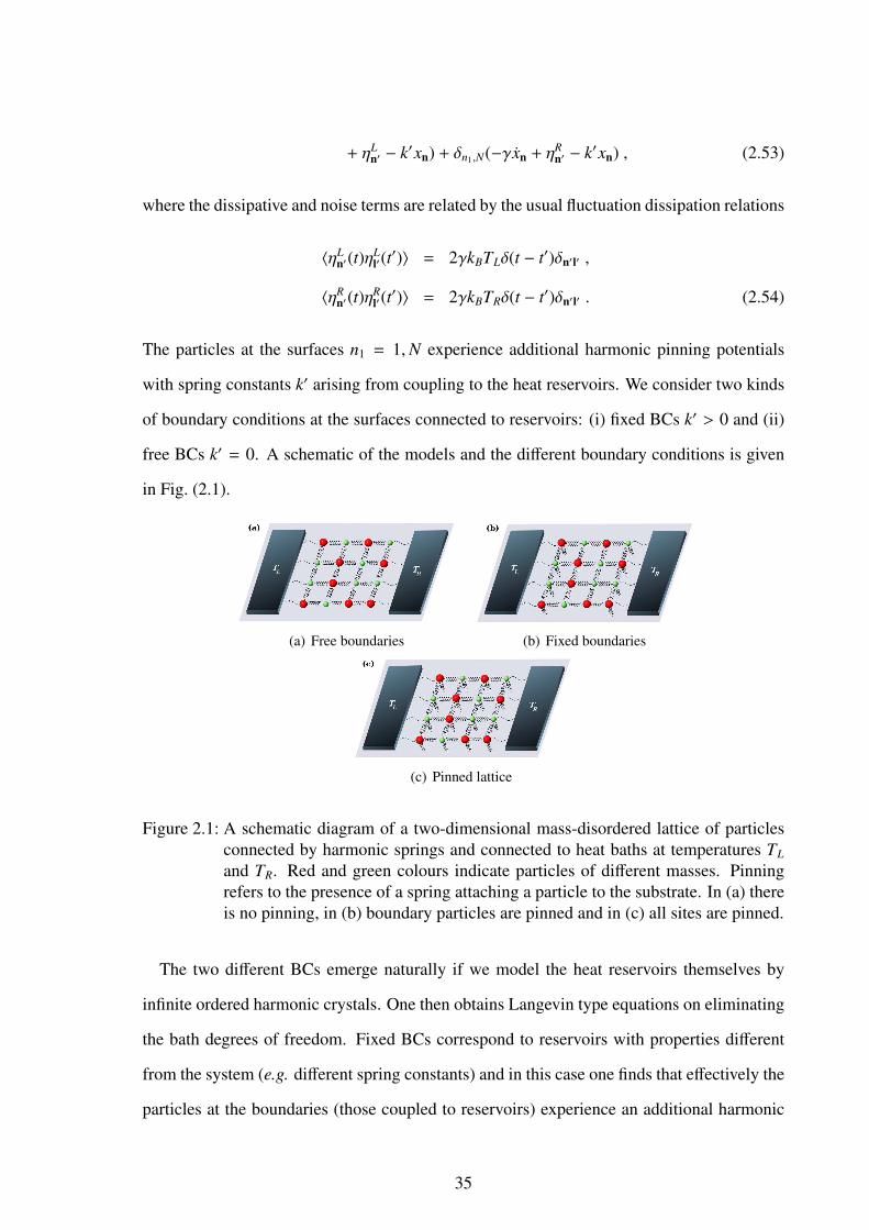
+ ηLn′ − k′xn) + δn1,N(−γxn + η
Rn′ − k′xn) , (2.53)
where the dissipative and noise terms are related by the usual fluctuation dissipation relations
〈ηLn′(t)η
Ll′(t′)〉 = 2γkBTLδ(t − t′)δn′l′ ,
〈ηRn′(t)η
Rl′(t′)〉 = 2γkBTRδ(t − t′)δn′l′ . (2.54)
The particles at the surfaces n1 = 1,N experience additional harmonic pinning potentials
with spring constants k′ arising from coupling to the heat reservoirs. We consider two kinds
of boundary conditions at the surfaces connected to reservoirs: (i) fixed BCs k′ > 0 and (ii)
free BCs k′ = 0. A schematic of the models and the different boundary conditions is given
in Fig. (2.1).
(a) Free boundaries (b) Fixed boundaries
(c) Pinned lattice
Figure 2.1: A schematic diagram of a two-dimensional mass-disordered lattice of particlesconnected by harmonic springs and connected to heat baths at temperatures TL
and TR. Red and green colours indicate particles of different masses. Pinningrefers to the presence of a spring attaching a particle to the substrate. In (a) thereis no pinning, in (b) boundary particles are pinned and in (c) all sites are pinned.
The two different BCs emerge naturally if we model the heat reservoirs themselves by
infinite ordered harmonic crystals. One then obtains Langevin type equations on eliminating
the bath degrees of freedom. Fixed BCs correspond to reservoirs with properties different
from the system (e.g. different spring constants) and in this case one finds that effectively the
particles at the boundaries (those coupled to reservoirs) experience an additional harmonic
35
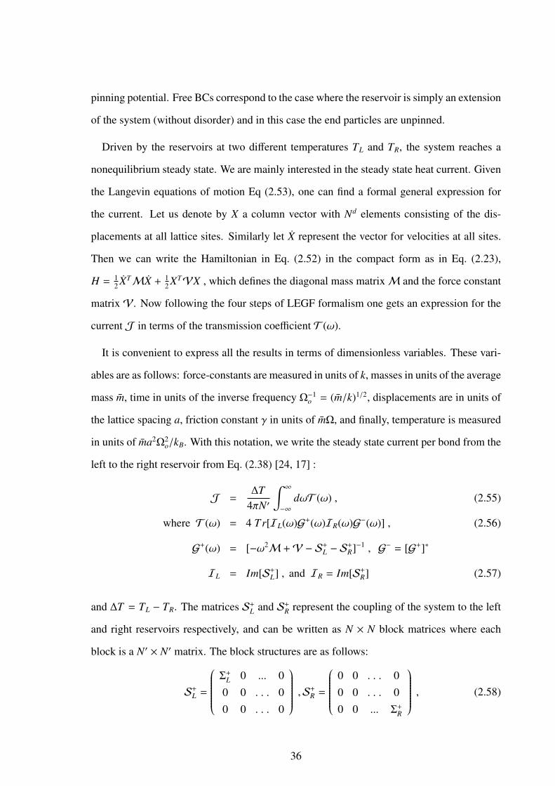
pinning potential. Free BCs correspond to the case where the reservoir is simply an extension
of the system (without disorder) and in this case the end particles are unpinned.
Driven by the reservoirs at two different temperatures TL and TR, the system reaches a
nonequilibrium steady state. We are mainly interested in the steady state heat current. Given
the Langevin equations of motion Eq (2.53), one can find a formal general expression for
the current. Let us denote by X a column vector with Nd elements consisting of the dis-
placements at all lattice sites. Similarly let X represent the vector for velocities at all sites.
Then we can write the Hamiltonian in Eq. (2.52) in the compact form as in Eq. (2.23),
H = 12 XTMX + 1
2 XTVX , which defines the diagonal mass matrixM and the force constant
matrix V. Now following the four steps of LEGF formalism one gets an expression for the
current J in terms of the transmission coefficient T (ω).
It is convenient to express all the results in terms of dimensionless variables. These vari-
ables are as follows: force-constants are measured in units of k, masses in units of the average
mass m, time in units of the inverse frequency Ω−1o = (m/k)1/2, displacements are in units of
the lattice spacing a, friction constant γ in units of mΩ, and finally, temperature is measured
in units of ma2Ω2o/kB. With this notation, we write the steady state current per bond from the
left to the right reservoir from Eq. (2.38) [24, 17] :
J =∆T
4πN′
∫ ∞
−∞
dωT (ω) , (2.55)
where T (ω) = 4 Tr[IL(ω)G+(ω)IR(ω)G−(ω)] , (2.56)
G+(ω) = [−ω2M +V − S+L − S+R]−1 , G− = [G+]∗
IL = Im[S+L] , and IR = Im[S+R] (2.57)
and ∆T = TL − TR. The matrices S+L and S+R represent the coupling of the system to the left
and right reservoirs respectively, and can be written as N × N block matrices where each
block is a N′ × N′ matrix. The block structures are as follows:
S+L =
Σ+L 0 ... 0
0 0 . . . 0
0 0 . . . 0
,S+R =
0 0 . . . 0
0 0 . . . 0
0 0 ... Σ+R
, (2.58)
36

where
Σ+L = Σ+R = iγωI , (2.59)
I is a N′×N′ unit matrix, and 0 is a N′×N′ matrix with all elements equal to zero. Similarly
the matricesM andV have the following block structure:
M =
M1 0 ... 0
0 M2 . . . 0
0 0 . . . 0
0 0 . . MN
, V =Φ −I . . . 0
−I Φ . . . 0
0 0 . . . 0
0 0 .. − I Φ
, (2.60)
where Mn denotes the diagonal mass-matrix for the n1 = n layer and Φ is a force-constant
matrix whose off-diagonal terms correspond to coupling to sites within a layer. Hence the
matrix G−1 = [−Mω2 +V − S+L − S+R] has the following structure:
[G]−1 =
a1 −I 0 ... 0
−I a2 −I 0 ... 0
... ... ... ... ...
0 ... 0 −I aN−1 −I
0 ... 0 −I aN
, (2.61)
where al = −Mlω2+Φ−δl,1Σ
+L−δl,NΣ
+R. With the form of S+L,R given in Eqs. (2.58)and (2.59),
we find that the expression for the transmission coefficient reduces to the following form:
T (ω) = 4 Tr[ΓL(ω)G+N(ω)ΓR(ω)G−N(ω)] ,
where ΓL,R = Im[Σ+L,R] (2.62)
and G+N is the (1,N)th block element of G and G−N = [G+N]†. We now show that G+N sat-
isfies some simple recursion relations and using those recursion relations the transmission
coefficient T (ω) can be expressed as a product of random matrices.
37
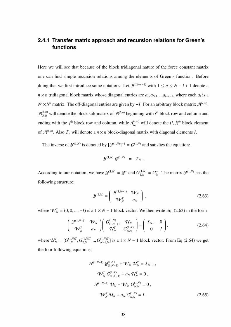
2.4.1 Transfer matrix approach and recursion relations for Green’sfunctions
Here we will see that because of the block tridiagonal nature of the force constant matrix
one can find simple recursion relations among the elements of Green’s function. Before
doing that we first introduce some notations. Let Y(l,l+n−1) with 1 ≤ n ≤ N − l + 1 denote a
n × n tridiagonal block matrix whose diagonal entries are al, al+1, ...al+n−1, where each al is a
N′×N′ matrix. The off-diagonal entries are given by −I. For an arbitrary block matrixA(l,m),
A(l,m)(i, j) will denote the block sub-matrix ofA(l,m) beginning with ith block row and column and
ending with the jth block row and column, while A(l,m)i, j will denote the (i, j)th block element
ofA(l,m). Also In will denote a n × n block-diagonal matrix with diagonal elements I.
The inverse of Y(1,N) is denoted by [Y(1,N)]−1 = G(1,N) and satisfies the equation:
Y(1,N) G(1,N) = IN .
According to our notation, we have G(1,N) = G+ and G(1,N)1,N = G+N . The matrix Y(1,N) has the
following structure:
Y(1,N) =
Y(1,N−1) WN
WTN aN
, (2.63)
whereWTN = (0, 0, ...,−I) is a 1 × N − 1 block vector. We then write Eq. (2.63) in the form Y(1,N−1) WN
WTN aN
G(1,N)(1,N−1) UN
UTN G(1,N)
N,N
= IN−1 0
0 I
, (2.64)
where UTN = [G(1,N)T
1,N ,G(1,N)T2,N ...,G(1,N)T
N−1,N] is a 1 × N − 1 block vector. From Eq (2.64) we get
the four following equations:
Y(1,N−1) G(1,N)(1,N−1) +WN U
TN = IN−1 ,
WTN G
(1,N)(1,N−1) + aN U
TN = 0 ,
Y(1,N−1) UN +WN G(1,N)N,N = 0 ,
WTN UN + aN G(1,N)
N,N = I . (2.65)
38
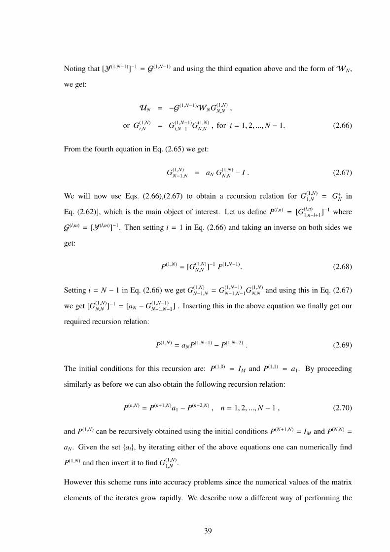
Noting that [Y(1,N−1)]−1 = G(1,N−1) and using the third equation above and the form ofWN ,
we get:
UN = −G(1,N−1)WNG(1,N)N,N ,
or G(1,N)i,N = G(1,N−1)
i,N−1 G(1,N)N,N , for i = 1, 2, ...,N − 1. (2.66)
From the fourth equation in Eq. (2.65) we get:
G(1,N)N−1,N = aN G(1,N)
N,N − I . (2.67)
We will now use Eqs. (2.66),(2.67) to obtain a recursion relation for G(1,N)1,N = G+N in
Eq. (2.62)], which is the main object of interest. Let us define P(l,n) = [G(l,n)1,n−l+1]−1 where
G(l,m) = [Y(l,m)]−1. Then setting i = 1 in Eq. (2.66) and taking an inverse on both sides we
get:
P(1,N) = [G(1,N)N,N ]−1 P(1,N−1). (2.68)
Setting i = N − 1 in Eq. (2.66) we get G(1,N)N−1,N = G(1,N−1)
N−1,N−1G(1,N)N,N and using this in Eq. (2.67)
we get [G(1,N)N,N ]−1 = [aN − G(1,N−1)
N−1,N−1] . Inserting this in the above equation we finally get our
required recursion relation:
P(1,N) = aN P(1,N−1) − P(1,N−2) . (2.69)
The initial conditions for this recursion are: P(1,0) = IM and P(1,1) = a1. By proceeding
similarly as before we can also obtain the following recursion relation:
P(n,N) = P(n+1,N)a1 − P(n+2,N) , n = 1, 2, ...,N − 1 , (2.70)
and P(1,N) can be recursively obtained using the initial conditions P(N+1,N) = IM and P(N,N) =
aN . Given the set ai, by iterating either of the above equations one can numerically find
P(1,N) and then invert it to find G(1,N)1,N .
However this scheme runs into accuracy problems since the numerical values of the matrix
elements of the iterates grow rapidly. We describe now a different way of performing the
39

recursion which turns out to be numerically more efficient. We first define
rN = P(1,N)[P(1,N−1)]−1 . (2.71)
From Eq. (2.69) we immediately get:
rN = aN −1
rN−1, (2.72)
with the initial condition r1 = a1. Then G(1,N)1,N is given by:
G(1,N)1,N = [P(1,N)]−1 = [rNrN−1...r1]−1
= r−11 r−1
2 ...r−1N . (2.73)
This form where at each stage r−1l is evaluated turns out to be numerically more accurate.
Finally, we show that one can express G(1,N)1,N in the form of a product of matrices. The
product form is such that the system and reservoir contributions are separated. First, we
note that the form of the matrices al for our specific problem is: al = cl − δl,1Σ1 − δl,NΣN
where cl = −Mlω2 + Φ. We define system-dependent matrices Q(1,n), Q(n,N) by replacing
a1, aN by c1, cN in the recursions for P’s. Thus Q(1,n) = P(1,n)(a1 → c1, aN → cN) and
Q(n,N) = P(n,N)(a1 → c1, aN → cN). Clearly Q’s satisfy the same recursion as the P’s with al
replaced by cl. Then using Eqs. (2.69),(2.70), and similar equations for the Qs’ we get:
P(1,N)
= Q(1,N) − Q(2,N) Σ1 − ΣN Q(1,N−1) + ΣN Q(2,N−1) Σ1
= (1 − ΣN)
Q(1,N) −Q(2,N)
Q(1,N−1) −Q(2,N−1)
1
Σ1
. (2.74)
From the recursion relations for the Qs’, it is easy to see that Q(1,N) −Q(2,N)
Q(1,N−1) −Q(2,N−1)
=
aN −I
I 0
Q(1,N−1) −Q(2,N−1)
Q(1,N−2) −Q(2,N−2)
= TNTN−1...T1 , (2.75)
40

where
Tl =
al −I
I 0
. (2.76)
From Eq. (2.74) we then obtain P(1,N) and from which we get G+N = [P(1,N)]−1. Using this and
noting that the baths are white noise Langevin baths we get
J =KB(TL − TR)
πN′
∫ ∞
−∞
dω ω2 γ2 Tr[[P+∗1,N(ω)P+T
1,N(ω)]−1]. (2.77)
Comparing the above equation with Eq. (2.55), we get
T (ω) = 4ω2 γ2 Tr[[P+∗1,N(ω)P+T
1,N(ω)]−1]. (2.78)
2.4.2 Current in one dimensional harmonic system:
For 1D chain the Hamiltonian in Eq. (2.52) looks like
H =N∑
l=1
[12
ml x2l +
12
kox2l
]+
N−1∑l=1
12
k(xl+1 − xl)2 +12
k′(x21 + x2
N) , (2.79)
and the corresponding langevin equations look like
m1 x1 = −(k′ + ko)x1 − k(x1 − x2) + γx1 + η1(t)
ml xl = −koxl − k(2xl − xl−1 − xl+1), 1 < l < N
mN xN = −(k′ + ko)xN − k(xN − xN−1) + γxN + ηN(t)
(2.80)
In the classical case, the steady state heat current from left to right reservoir is obtained from
Eq. (2.77) [17, 13]
where TN(ω) = γ2ω2|GN |2 ,
GN(ω) = [P(1,N)]−1(ω),
Vlm = (1 + k′ + ko) δl,m − δl,m−1 for l = 1 ,
41
= −δl,m+1 + (2 + ko) δl,m − δl,m−1 for 2 ≤ l ≤ N − 1 ,
= (1 + k′ + ko) δl,m − δl,m+1 for l = N ,
Σlm = iγωδlm[δl1 + δlN] ,
All the variables and parameters in the above expressions are now dimensionless quantities
and [P(1,N)]−1 is now just a complex number. It is easy to identify that
P(1,N) = ∆N (2.81)
where ∆N is the determinant of the matrix Z = [−ω2M +V − Σ].
Disordered case: This has been extensively studied and is well understood [14, 15, 17,
19, 22, 69]. The matrix formulation explained in the last section leads to a clear analytic
understanding of the main results. From the products of N random matrices of size (2 × 2)
one calculates P(1,N) numerically and hence T (ω). Clearly T (ω) and J will be different for
different disorder realisations. Since we will mostly be interested in disorder averages of
these quantities we need to introduce some notation for the disorder average. We consider
[x] to be the disorder average of the quantity x. We denote disordered averaged TN(ω) and
J by T (ω) = [T ] and J = [J] respectively.
There are three observations that enable one to determine the asymptotic system size de-
pendence of the current. These are:
(i)P(1,N) = [G+N]−1 given by Eqs. (2.74), (2.76) is a complex number which can be expressed
in terms of the product of N random 2 × 2 matrices. Using Furstenberg’s theorem it can
be shown that for almost all disorder realizations, the large N behaviour of P(1,N) for fixed
ω > 0 is |P(1,N)| ∼ ebNω2, where b > 0 is a constant. This is to be understood in the sense that
limN→∞(1/N) log |P1,N)| ∼ bω2 for ω → 0. Since T (ω) ∼ |P(1,N)|−2 ∼ e−2bNω2, this implies
that transmission is significant only for low frequencies ω <∼ ωc(N) ∼ 1/N1/2. The current is
therefore dominated by the small ω behaviour of T (ω).
(ii) The second observation made in [19] is that the transmission for ω < ωc(N) is ballistic
in the sense that T (ω) is insensitive to the disorder. This can be seen in fig. (2.2) where the
42

0 0.025 0.05 0.075 0.1ω
1
10
100
1000
10000
1e+05
1e+06<
|Q(1
,N) |2 >
DisorderedOrdered
Figure 2.2: Frequency dependence of [|Q(1,N)|] at small ω for ∆ = 0.2 and N = 1024 withfixed BC is compared with the same for an ordered chain. In disordered case|Q(1,N)|2 is averaged over 104 different realisation of masses.
disorder average of |Q(1,N)|2 for a chain of length N = 1024 is plotted along with the same
for an ordered chain.
(iii) The final important observation is that the form of the prefactors of e−bNω2in T (ω) for
ω < ωc(N) depends strongly on boundary conditions and bath properties [19, 22]. For the
white noise Langevin baths, one finds T (ω) ∼ ω2e−bNω2for fixed BC and T (ω) ∼ ω0e−bNω2
for free BC [22]. This difference arises because of the scattering of long wavelength modes
by the boundary pinning potentials. Now, the asymptotic N dependence of the disorder
averaged current in the NESS will be
J ∼
∫ ωc(N)
0T (ω)
∼ N−12 for free BC
∼ N−32 for fixed BC. (2.82)
In Fig. (2.3), we plot numerical results showing T (ω) for the 1D mass-disordered lattice
with both fixed and free boundary conditions. We consider a binary mass disordered crystal
43

0 0.5 1 1.5 2ω
0
0.2
0.4
0.6
0.8
1T
(ω)
0 0.5 1 1.5 2ω
0
0.1
0.2
0.3
0.4
T(ω
)
Figure 2.3: 1D unpinned case with both free and fixed (INSET) boundary conditions: plotof the disorder averaged transmission T (ω) versus ω for ∆ = 0.4. The variouscurves (from top to bottom) correspond to lattices of sizes N = 64, 256, 1024respectively.
in which we set the masses of exactly half the particles at randomly chosen sites to be m −∆
and the rest to be m+∆. Thus ∆ gives a measure of the disorder. One can clearly see the two
features discussed above, namely (i) dependence of frequency cut-off on system size and (ii)
dependence of the form of T (ω) on boundary conditions. Using the three observations made
above it is easy to arrive at the conclusion that J ∼ N−3/2 for fixed BC and J ∼ N−1/2 for free
BC. In the presence of a pinning potential the low-frequency modes are suppressed and one
obtains a heat insulator with J ∼ e−cN , with c a constant [69] (see also [21] and references
therein).
Ordered case: In this case, masses of all the particles are the same (say, m). Hence one
can write a closed form expression for ∆N . After some straightforward calculations and
rearrangements one can show that [11]:
∆N = [a(q) sin Nq + b(q) cos Nq]/ sin q , (2.83)
44

where a(q) = [2 − γ2ω2 + k′2 − 2k′] cos q + 2k′ − 2 − 2iγω[1 + (k′ − 1) cos q] ,
b(q) = [γ2ω2 − k′2 + 2k′] sin q + 2iγω(k′ − 1) sin q ,
2 cos q = −mω2 + ko + 2 . (2.84)
From the relation in Eq. (2.84), it is clear that for frequencies outside the phonon band
ko ≤ mω2 ≤ ko + 2 the wave vector q becomes imaginary and hence, from Eq. (2.83), we
note that the transmission coefficient T (ω) decays exponentially with N. Hence, for large N
we need to consider only the range 0 < q < π and the current is given by:
JC =2γ2(TL − TR)
π
∫ π
0dq|
dωdq|ω2
q
|∆N |2 , (2.85)
with mω2q = ko +2[1− cos (q)]. We now state the following result. For any two well-behaved
functions g1(q) and g2(q)
limN→∞
∫ π
0dq
g1(q)1 + g2(q) sin Nq
=
∫ π
0dq
g1(q)[1 − g2
2(q)]1/2. (2.86)
There are three steps required to prove this result: (i) expand the factor 1/[1+g2(q) sin (Nq)]
(valid for |g| < 1 in the integration range), (ii) take the N → ∞ limit, (iii) resum the resulting
series. It is easy to see that the Eq. (2.85) has the same structure as the left hand side of
Eq. (2.86) once we note that ∆N can be written as
|∆N |2 = (|a|2 + |b|2)[1 + r sin(2Nq + φ)]/[2 sin2 (q)]
where r cos φ = (ab∗ + a∗b)/(|a|2 + |b|2)
and r sin φ = (|b|2 − |a|2)/(|a|2 + |b|2). (2.87)
Hence using Eq. (2.86) and simplifying, we get [22]:
JC =γk2kB(TL − TR)
πm
∫ π
0
sin2 q dqΛ −Ω cos q
=γk2kB(TL − TR)
mΩ2 (Λ −√Λ2 −Ω2) , (2.88)
where Λ = 2k(k − k′) + k′2 +(ko + 2k)γ2
mand Ω = 2k(k − k′) +
2kγ2
m.
45

2.4.3 Current in d-dimensional ordered harmonic system
The current in a d-dimensional ordered lattice can be calculated by using the observation that
the problem of heat conduction in a d-dimensional ordered harmonic lattice can be related
to heat conduction across Nd−1 independent ordered harmonic chains with different onsite
potentials. Hence the transmission coefficient T (ω) for the d-dimensional lattice can be
expressed as a sum of the transmission coefficients of the 1D chains. Now we will see how
one can relate the d-dimensional problem to a one dimensional problem. The Hamiltonian
of the d-dimensional system is given in sec. (2.4). We recall that xn is the displacement
of a particle at the lattice site n = (n1,n′). Let us consider that for each n there exists a
q = (q1, q2, ..., qd−1, qd) = (q1,q′) with qα = 2πlN where l goes from 1 to N such that
1Nd−1
∑q′
eiq′.n′1 eiq′.n′2 = δn′1,n′2
(2.89)
Now, if we define
xn1(q′) =
1
Nd−1
2
∑n′
x(n1,n′) eiq′.n′ , (2.90)
then one can show that, for each q′, xn1(q′) satisfies a Langevin equation corresponding to a
one-dimensional Hamiltonian with the onsite spring constant replaced by
λ(q′) = ko + 2k(d − 1 −∑
α=2,..,d
cos qα). (2.91)
Hence in the ordered case the d-dimensional harmonic system can be decomposed into Nd−1
harmonic chains. For N → ∞, the heat current J(q′) for each mode with given q′ is then
simply given by Eq.(2.88) with ko replaced by λ(q′). The heat current per bond is then given
by:
J =1
Nd−1
∑q′
J(q′) . (2.92)
The above result also holds for finite lengths in the transverse direction. For infinite trans-
46

verse lengths, we get J =∫...
∫ 2π
0dqJ(q)/(2π)d−1 . Heat conduction in higher dimensional
disordered harmonic systems is studied in the next chapter.
47
3 Study on heat conduction in higherdimensional harmonic system
In the previous chapter we have discussed the LEGF formalism and applied it to one dimen-
sional harmonic chain to find out the system size dependence of the NESS current J. We also
mentioned results on heat conduction in one dimensional systems, from which we conclude
that system size scaling of the NESS current strongly depends on the boundary conditions
and also on the presence of pinning potentials. There have been theoretical as well as com-
putational studies on finding the system size dependence of heat current in NESS. All the
studies suggest that Fourier’s law is not valid in one and two dimensional systems, even in
the presence of anharmonic interactions, unless the system is also subjected to an external
substrate pinning potential. It is generally expected that the system size scaling of J will
be less sensitive to boundary conditions as we go to higher and higher dimensions. Based
on empirical evidence, it is also expected that average energy current J in NESS through
a system in a slab geometry, should be proportional to N−1. In this chapter we present nu-
merical studies on heat conduction through disordered harmonic lattices in two and three
dimensions.
Here we report results of heat conduction studies in 2D and 3D disordered harmonic lat-
tices with scalar displacements and connected to heat baths modeled by Langevin equations
with white noise. In crystalline solids the carriers of heat are phonons, which are normal
modes of lattice vibrations. Transport properties of these modes will be affected by Ander-
son localization [70] and by phonon scattering in anharmonic lattices. We pay particular
attention to the interplay between localization effects, boundary effects, and the role of long
wavelength modes. The steady state heat current is given exactly as an integral over all fre-
48
quencies of a phonon transmission coefficient as shown in Eq. (2.38). Using this formula
and heuristic arguments, based on localization theory and kinetic theory results, we estimate
the system size dependence of the current.
Numerically we use two different approaches to study the nonequilibrium stationary state.
The first is a numerical one which relies on the result that the current can be expressed in
terms of a transmission coefficient. We saw in Eq. (2.38) that the transmission coefficient can
be written in terms of phonon Green’s functions. Using the recursion relations of the Green’s
functions (discussed in sec. (2.4.1) we implement efficient numerical schemes to evaluate this
transmission coefficient. The second approach is through direct nonequilibrium simulations
of the Langevin equations of motion and finding the steady state current and temperature
profiles. We have also studied properties of the isolated system, i.e., of the disordered lattice
without coupling to heat baths, and looked at the normal mode frequency spectrum and the
wavefunctions. One measure of the degree of localization of the normal modes of the isolated
system is the so-called inverse participation ratio [IPR, defined in Eq. (3.11) below]. We have
carried out studies of the IPR and linked these with results from the transmission study.
The rest of the chapter is organized as follows. In Sec. (3.1) and Sec. (3.2) we discuss ear-
lier studies on phonon localization and kinetic theory results in phonon transport respectively.
In the beginning of Sec. (3.3) we describe the specific model studied which is followed by
discussions on quantities studied and approaches used in this chapter. Heuristic arguments
and our predictions on asymptotic system size dependence of current are given in Sec. (3.4).
In Sec. (3.5) we present results from both the numerical approach and from nonequilibrium
simulations which is followed by conclusion in Sec. (3.6).
3.1 Phonon localization
This is closely related to the electron localization problem. The effect of localization on
linear waves in disordered media has been most extensively studied in the context of the
Schrodinger equation for non-interacting electrons moving in a disordered potential. Look-
ing at the eigenstates and eigenfunctions of the isolated system of a single electron in a
49
disordered potential one finds that, in contrast to the spatially extended Bloch states in pe-
riodic potentials, there are now many eigenfunctions which are exponentially localized in
space. It was argued by Mott and Twose [73] and by Borland [74], and proven rigorously
by Goldsheid et al. [75], that in one dimension all states are exponentially localized. In two
dimensions there is no proof but it is believed that again all states are localized. In three
dimensions there is expected to be a transition from extended to localized states as the en-
ergy is moved towards the band edges [76]. The transition from extended to localized states,
which occurs when the disorder is increased, changes the system from a conductor to an
insulator. The connection between localization and heat transport in a crystal is complicated
by the fact that phonons of all frequencies can contribute to energy transmission across the
system. In particular, account has to be taken of the fact that low frequency phonon modes
are only weakly affected by disorder and always remain extended. The heat current carried
by a mode which is localized on a length scale `, decays with system length N as e−N/`. This
` depends on the phonon frequency, and low frequency modes for which ` ∼ N will there-
fore be carriers of the heat current. The net current then depends on the nature of these low
frequency modes and their scattering due to boundary conditions (BCs).
A renormalization group study in a disordered continuum elastic media by John et al. [17]
found that in 1D and 2D all non-zero frequency phonons are localized. They studied the
spreading of an energy pulse to define a frequency dependent diffusivity D0(ω). From the
behaviour of D0(ω) under renormalization one can obtain a differential recursion relation for
the resistivity. This relation shows that in the large system size limit the RG flow is towards
infinity for dimensions ≤ 2, in contrast to d = 3 where the flow is towards zero as long as ω is
less than some fixed value, independent of system size. Hence all finite-frequency modes in
one and two dimensions are localized. From the differential recursion relations one finds that
for d = 1 and d = 2 the localization length in ω → 0 limit diverges as ∼ 1/ω2 and ∼ e1/ω2
respectively. In 3D there exists a frequency, independent of system size, above which all
states are localized while states below that frequency are extended. Hence for a system of
size N there will be a cut-off frequency ωLc (which depends on N for d ≤ 2) above which all
50
the modes are localized. In different dimensions ωLc is given by
ωLc ∼ N−1/2 for d = 1
∼ [log(N)]−1/2 for d = 2
∼ nonzero value independent of N for d = 3 (3.1)
However this study does not make any statements on the system size dependence of the
conductivity.
3.2 Kinetic theory
If one considers the low frequency extended phonons, then the effect of disorder is weak and
in dimensions d > 1 one expects that localization effects can be neglected and kinetic theory
should be able to provide an accurate description. In this case one can think of Rayleigh
scattering of phonons. This gives an effective mean free path `K(ω) ∼ ω−(d+1) [see chapter
(1)] , for dimensions d > 1, and a diffusion constant D(ω) = v`K(ω) where v, the sound
velocity, can be taken to be constant. For a finite system of linear dimension N we have
D(ω) = vN for ω <∼ N−1/(d+1). Kinetic theory then predicts
κ =
∫ ωmax
N−1dωρ(ω)D(ω) , (3.2)
where ρ(ω) ∼ ωd−1 is the density of states and we get κ ∼ N1/(d+1), implying µ = d/(d + 1).
The divergence of the phonon mean free path at low frequencies and the resulting diver-
gence of the thermal conductivity of a disordered harmonic crystal has been discussed in the
literature and it has been argued that anharmonicity is necessary to make κ finite [77, 2].
3.3 System and methods
Here we consider heat conduction across a d-dimensional hyper-cubic lattice which is con-
nected to two Langevin heat baths at the two ends of it. The model was defined in Sec. (2.4)
in detail. For completeness, we recall the Hamiltonian of the system and the corresponding
51

Langevin equations. The Hamiltonian of the system is given by
H =∑
n
12
mn x2n +
N−1∑n1=1
∑n′,e
k2
(xn − xn+e)2
+ko
2
∑n
x2n +
k′
2
∑n′
x2(1,n′) +
k′
2
∑n′
x2(N,n′) , (3.3)
and the Langevin equation are given by
mn xn = −∑
e
k(xn − xn+e) − koxn + δn1,1(−γxn
+ ηLn′ − k′xn) + δn1,N(−γxn + η
Rn′ − k′xn) . (3.4)
The meaning of all the variables and quantities appearing in the above two equations is
explained in sec. (2.4). For a particular disorder configuration the steady state current per
bond from left to right reservoir has the following form ( Eq. (2.55) )
J =∆T
4πN′
∫ ∞
−∞
dωT (ω) , (3.5)
where
T (ω) = 4 Tr[IL(ω)G+(ω)IR(ω)G−(ω)] , (3.6)
G+(ω) = [−ω2M +V − S+L − S+R]−1 , G− = [G+]∗
IL = Im[S+L] , and IR = Im[S+R] (3.7)
and ∆T = TL − TR. The specific form of S+L,R for our system described by Eqs. (3.4) was
given in Eq. (2.58). The matrix G+(ω) can be identified as the phonon Green’s function of
the system with self-energy corrections due to the baths [24]. The integrand in Eq. (3.5)
T (ω) can be thought of as the transmission coefficient of phonons at frequency ω from the
left to the right reservoir. It will vanish, when N → ∞ , at values of ω for which the disorder
averaged density of states is zero. Note that due to the harmonic nature of the forces the
dependence of the heat flux on the reservoir temperatures enters only through the term ∆T
in Eq. (3.5).
52
Numerical approach: In sec 2.4.1, we have described how T can be expressed in a
form amenable to accurate numerical computation. The system sizes we study are suffi-
ciently large so that T (ω) has appreciable values only within the range of frequencies of
normal modes of the isolated system, i.e., corresponding to γ = 0 in the equation of motion
( Eq. (2.53) ). Outside this range we find that the transmission rapidly goes to zero. By
performing a discrete sum over the transmitting range of frequencies we do the integration
in Eq. (3.5) to obtain the heat current density J . In evaluating the discrete sum over ω, step
sizes of δω = 0.01 − 0.0001 are used and we verified convergence in most cases. With our
choice of units we have k = 1, m = 1 and we fixed ∆T = 1. Different values of the mass
variance ∆ and the on-site spring constant ko were studied for two and three dimensional
lattices of different sizes. It is expected that the value of the exponent µ will not depend on γ
and in our calculations we mostly set γ = 1, except when otherwise specified.
Simulation approach: The simulations of Eq. (3.4) are performed using a velocity-Verlet
scheme as given in [78]. The current and temperature profiles in the system are obtained
from the following time averages in the nonequilibrium steady state:
J1 =1N′
∑n′
γ
m(1,n′)
[TL − m(1,n′)〈x2
(1,n′)〉],
Jn = −1N′
∑n′〈 [x(n,n′) − x(n−1,n′)] x(n,n′) 〉 ,
n = 2, 3, ...,N ,
JN+1 = −1N′
∑n′
γ
m(N,n′)
[TR − m(N,n′)〈x2
(N,n′)〉],
Tn =1N′
∑n′
m(n,n′)〈 x2(n,n′) 〉 , n = 1, 2, ...,N .
We then obtained the average current J = (∑N+1
n=1 JN)/(N + 1). In the steady state one has
Jn = J for all n and stationarity can be tested by checking how accurately this is satisfied.
We chose a step size of ∆t = 0.005 and equilibrated the system for over 108 time steps.
Current and temperature profiles were obtained by averaging over another 108 time steps.
The parameters TL = 2.0,TR = 1.0 are kept fixed and different values of the mass variance ∆
and the on-site spring constant ko are simulated.
53

Disorder averaged Tn is denoted by [Tn]. Note that disorder average of any quantity is
denoted by [...]. We also define the disorder averaged transmission per bond with the notation
T (ω) =1N′
[T (ω)] . (3.8)
Numerical analysis of eigenmodes and eigenfunctions: We have studied the proper-
ties of the normal modes of the disordered harmonic lattices in the absence of coupling to
reservoirs, again with both free and fixed boundary conditions. The d-dimensional lattice
has p = 1, 2, ...,Nd normal modes and we denote the displacement field corresponding to
the pth mode by an(p) and the corresponding eigenvalue by ω2p. The normal mode equation
corresponding to the Hamiltonian in Eq. (3.3) is given by:
mnω2pan = (2d + ko)an −
∑e
an+e , (3.9)
where the an satisfy appropriate boundary conditions. Introducing variables ψn(p) =
m1/2n an(p), vn = (2d + ko)/mn and tn,l = 1/(mnml)1/2 for nearest neighbour sites n, l the
above equation transforms to the following form:
ω2pψn(p) = vnψn(p) −
∑l
tn,lψl(p) . (3.10)
This has the usual structure of an eigenvalue equation for a single electron moving in a
d-dimensional lattice corresponding to a tight-binding Hamiltonian with nearest neighbour
hopping tn,l and on-site energies vn. Note that tn,l and vn are correlated random variables,
hence the disorder-energy diagram might differ considerably from a single band Anderson
tight-binding model.
We have numerically evaluated all eigenvalues and eigenstates of the above equation for
finite cubic lattices of size upto N = 64 in 2D and N = 16 in 3D. One measure of the degree
of localization of a given mode is the inverse participation ratio (IPR) defined as follows:
P−1 =
∑n a4
n
(∑
n a2n)2 . (3.11)
For a completely localized state, i.e. an = δn,n0 , P−1 takes the value 1. On the other hand for
54

a completely delocalized state, for which an = N−d/2ein.q where q is a wave vector, P−1 takes
the value N−d. We will present numerical results for the IPR calculated for all eigenstates of
given disorder realizations, in both 2D and 3D. Finally we will show some results for the
density of states, ρ(ω), of the disordered system defined by:
ρ(ω) =∑
p
δ(ωp − ω) . (3.12)
The density of states of disordered binary mass harmonic crystals was studied numerically
by Payton and Visscher in 1967 [80] and reviewed by Dean in 1972 [81].
20
40
60
20
40
60
-1-0.5
00.51
20
40
60
Ballistic
(a)
20
40
60
20
40
60
-5
0
5
20
40
60
Diffusive
(b)
20
40
60
20
40
60
02.55
7.510
20
40
60
Localized
(c)
Figure 3.1: Three different types of modes
3.4 Heat conduction in disordered harmonic crystals:General considerations
Here we will try to extend the analysis of the 1D case (given in the previous chapter) to
higher dimensions. For this we will use inputs from both kinetic theory and the theory of
phonon localization. The main point of our arguments involves the assumption that normal
modes can be classified as ballistic, diffusive or localized. The classification refers both
to the character of the eigenfunctions as well as to their transmission properties. Ballistic
55
modes are spatially extended and approximately periodic; their transmission is independent
of system size. Diffusive modes are extended but non-periodic and their transmission decays
as 1/N. For localized modes transmission decays exponentially with N. In the context of
kinetic theory calculations, the ballistic modes are the low frequency modes with phonon
mean free path `K(ω) >∼ N, and their contribution to the current leads to divergence of the
thermal conductivity. Here we carefully examine the effect of both free and fixed boundary
conditions on these modes.
In the presence of an external pinning potential low frequency modes are suppressed,
hence one expects qualitative differences in transport properties. The pinned system has often
been used as a model system to study the validity of Fourier’s law. It has no translational
invariance and is thus more closely related to the problem of electrons moving in a random
potential. Using localization theory we determine the frequency region where states are
localized. The lowest frequency states with ω→ 0 will be ballistic and we use kinetic theory
to determine the fraction of extended states which are ballistic. We assume that at sufficiently
low frequencies the effective disorder is always weak (even when the mass variance ∆ is
large) and one can still use kinetic theory. Corresponding to the three observations made
above for the 1D case we now make the following arguments:
(i) From localization theory one expects all fixed non-zero frequency states in a 2D dis-
ordered system to be localized when the size of the system goes to infinity. As discussed
in Sec. (3.1), localization theory gives us a frequency cut-off ωLc = (ln N)−1/2 in 2D above
which states are localized. In 3D one obtains a finite frequency cut-off ωLc independent of
system size above which states are localized.
(ii) For the unpinned case with finite N there will exist low frequency states below ωLc ,
in both 2D and 3D, which are extended states. These states are either diffusive or ballistic.
Ballistic modes are insensitive to the disorder and their transmission coefficients are almost
the same as for the ordered case. To find the frequency cut-off below which states are ballistic
we use kinetic theory results (see Sec. (1.1.2)). For the low-frequency extended states we
expect kinetic theory to be reliable and this gives us a mean free path for phonons `K ∼
56

ωKc
ωL
c
ωBallistic Diffusive Localized
Figure 3.2: Frequency spectrum
ω−(d+1). This means that for low frequencies ω <∼ ωK
c = N−1/(d+1) we have `K(ω) > N and
phonons transmit ballistically. We now proceed to calculate the contribution of these ballistic
modes to the total current. This can be obtained by looking at the small ω form of TN(ω)
for the ordered lattice. States with frequency lying between [ωKc , ω
Lc ] are assumed to be
diffusive while making predictions about the system size dependence of current. Fig. (3.2)
schematically describes the nature of the modes at different ranges.
(iii) For the ordered lattice T (ω) is typically a highly oscillatory function with the oscilla-
tions increasing with system size. An effective transmission coefficient in the N → ∞ limit
can be obtained by considering the integrated transmission. This asymptotic effective low-
frequency form of T (ω), for the ordered lattice can be calculated using methods described in
[22] and is given by:
T (ω) ∼ ωd+1 , fixed BC
T (ω) ∼ ωd−1 , free BC , (3.13)
the result being valid for d = 1, 2, 3 [82].
Using the above arguments we then get the ballistic contribution to the total current density
(for the unpinned case) as:
Jball ∼
∫ ωKc
0dω ωd+1 ∼
1N(d+2)/(d+1) , fixed BC,
∼
∫ ωKc
0dω ωd−1 ∼
1Nd/(d+1) , free BC . (3.14)
We can now make predictions for the asymptotic system size dependence of total current
density in two and three dimensions.
Two dimensions: From localization theory one expects that all finite frequency modesω >∼
57
ωLc = (ln N)−1/2 are localized and their contribution to the total current falls exponentially
with system size. Our kinetic theory arguments show that the low frequency extended states
withωKc
<∼ ω
<∼ ωL
c are diffusive (whereωKc = N−1/3) while the remaining modes withω <
∼ ωKc
are ballistic. The diffusive contribution to total current will then scale as Jdiff ∼ (ln N)−1/2N−1.
The ballistic contribution depends on BCs and is given by Eq. (3.14). This gives Jball ∼ N−4/3
for fixed BC and Jball ∼ N−2/3 for free BC. Hence, adding all the different contributions, we
conclude that asymptotically:
J ∼1
(ln N)1/2N, fixed BC, d = 2 ,
∼1
N2/3 , free BC, d = 2. (3.15)
In the presence of an onsite pinning potential at all sites the low frequency modes get cut off
and all the remaining states are localized, we expect:
J ∼ e−bN , pinned , d = 2 , (3.16)
where b is some positive constant.
Three dimensions: In this case localization theory tells us that modes with ω>∼ ωL
c are
localized and ωLc is independent of N. From kinetic theory we find that the extended states
with ωKc
<∼ ω
<∼ ωL
c are diffusive (with ωKc = N−1/4) and those with ω <
∼ ωKc are ballistic.
The contribution to current from diffusive modes scales as Jdiff ∼ N−1. The ballistic contri-
bution (from states with ω <∼ N−1/4) is obtained from Eq. (3.14) and gives Jball ∼ N−5/4 for
fixed BC and Jball ∼ N−3/4 for free BC. Hence, adding all contributions, we conclude that
asymptotically:
J ∼1N, fixed BC , d = 3 ,
∼1
N3/4 , free BC , d = 3 . (3.17)
In the presence of an onsite pinning potential at all sites the low frequency modes get cut
off and, since in this case the remaining states form bands of diffusive and localized states,
58

0 1 2 3 4 50
1
2
[ρ(ω
)]
1D: Disordered1D: Ordered
0 1 2 3 4 5 6 70
0.5
1 2D: Disordered2D: Ordered
0 1 2 3 4 5 6 7 8ω
0
0.5
1 3D: Disordered3D: Ordered
Figure 3.3: Unpinned lattices with fixed BC in one direction and periodic BC in all others.Disorder averaged density of states obtained numerically from the eigenvalues ofseveral disorder realizations in 1D, 2D and 3D for lattice sizes N = 4096, 64, 16respectively. Note that the low frequency behaviour is unaffected by disorder andone has ωd−1 as ω → 0. We set ∆ = 0.8, k = 1 and averaged over 30 realizationsin 1D and over 10 realizations in 2D and 3D. In 2D and 3D there is not muchvariation in ρ(ω) for different disorder samples. Also shown are the density ofstates for the binary mass ordered lattices.
hence we expect:
J ∼1N, pinned , d = 3. (3.18)
Thus in 3D both the unpinned lattice with fixed boundary conditions and the pinned lattice
are expected to show Fourier type of behaviour as far as the system size dependence of the
current is concerned.
Note that for free BC, the prediction for the current contribution from the ballistic part
Jball ∼ N−d/(d+1) is identical to that from kinetic theory discussed earlier. This agreement can
be traced to the small ω form of T (ω) ∼ ωd−1 for free BC [see Eq. (3.13)] which is identical
to the form of the density of states ρ(ω) used in kinetic theory. The typical form of density of
59

3 4 5 6 7 8 90
1
2
3
1D: Disordered1D: Ordered
3 3.5 4 4.5 5 5.50
0.51
1.52
[ρ(ω
)]
2D: Disordered2D: Ordered
3 4 5 6 7 8 9 10 ω
00.5
11.5
23D: Disordered3D: Ordered
Figure 3.4: Pinned lattices: Disorder averaged density of states obtained numerically fromthe eigenvalues of several disorder realizations in 1D, 2D and 3D for lattice sizesN = 4096, 64, 16 respectively. Note that low frequency modes are absent. Weset k = 1, ko = 10.0 and ∆ = 0.4 in 2D and ∆ = 0.8 in 1D, 3D. Averages weretaken over 30 realizations in 1D and 10 realizations in 2D, 3D. We find that in2D and 3D there is not much variation in ρ(ω) for different disorder samples.Also shown are the density of states for the binary mass ordered lattices.
states for ordered and disordered lattices in different dimensions is shown in Fig. (3.3) and
we can see that the low frequency form is similar in both cases and has the expected ωd−1
behaviour. However it seems reasonable to expect that, since the transport current phonons
are injected at the boundaries, in kinetic theory one needs to use the local density of states
evaluated at the boundaries. For fixed BC this will then give rise to an extra factor of ω2
(from the squared wavefunction) and then the kinetic theory prediction matches with those
given above.
We note that the density of states in Fig. (3.3) show apparent gaps in the middle ranges
of ω for d = 2, 3. These might be expected to disappear when the size of the system goes
to infinity when there should be large regions containing only masses of one type [17, 69].
60

These regions will however be rare. In Fig. (3.4) we show plots of the density of states for the
ordered and disordered harmonic lattices in the presence of pinning. In this case the gaps in
the spectrum are more pronounced and, for large enough values of ko and ∆, may be present
even in the thermodynamic limit.
3.5 Results from Numerics and Simulations
We now present the numerical and simulation results for transmission coefficients, heat cur-
rent density, temperature profiles and IPRs for the disordered harmonic lattice in various
dimensions. The numerical scheme for calculating J is both faster and more accurate than
nonequilibrium simulations. Especially, for strong disorder, equilibration times in nonequi-
librium simulations become very large and in such cases only the numerical method can be
used. However we also show some nonequilibrium simulation results. Their almost perfect
agreement with the numerical results provides additional confidence in the accuracy of our
results. In Sec. (3.5.1) we give the results for the 2D lattice for the unpinned case with both
fixed and free boundary conditions and then for the pinned case. In Sec. (3.5.2) we present
the results for the three dimensional case with and without substrate pinning potentials.
3.5.1 Results in two dimensions
In this section we consider N × N square lattices with periodic BCs in the ν = 2 direction
and either fixed or free BCs in the conducting direction (ν = 1). One of the interesting
questions here is as to how the three properties for the 1D case discussed in second chapter
get modified for the 2D case.
3.5.1.1 Disordered 2D lattice without pinning
Fixed BC: we have computed the transmission coefficients and the corresponding heat cur-
rents for different values of ∆ and for system sizes from N = 16 − 1024. The number of
averages varied from over 100 samples for N = 16 to about two samples for N = 1024.
In Figs. (3.5,3.6,3.7) we plot the disorder averaged transmission coefficient for three differ-
61

0 0.25 0.5 0.75 1 1.25 1.5 1.75ω
0
2
4
6
8
10
N T
(ω)
N=64N=128N=256N=512N=1024
0 0.25 0.5 0.75 1 1.25 1.5 1.750
0.02
0.04T
(ω)
N=64N=128N=256N=512N=1024
(i)
(ii)
0 2 4 6 8 10 12ω
1
10
100
1000
N2 P
-1
N=32N=64
0 2 4 6 8 10 120
0.5
1
ρ(ω
) Ordered latticeDisordered lattice
(iii)
(iv)
Figure 3.5: 2D unpinned case with fixed BC for ∆ = 0.95. (i) Plot of the disorder averagedtransmission T (ω) versus ω. (ii) Plot of NT (ω). The range of frequencies forwhich T (ω) ∼ 1/N is indicated by the dashed line. (iii) Plot of ρ(ω) for binarymass ordered and single disordered sample. (iv) Plot of N2P−1 for single samples(smoothed data). We see that even though the allowed normal modes occur overa large frequency band ≈ (0 − 12), transmission takes place in a small band≈ (0 − 1.25) and is negligible elsewhere. The IPR plots confirm that the non-transmitting states correspond to localized modes. In (i) we see that ωL
c is slowlydecreasing with inrease of N.
62

ent disorder strengths, ∆ = 0.95, ∆ = 0.8 and ∆ = 0.2, for different system sizes. The
corresponding plots of IPRs as a function of normal mode frequency ωp, for single disorder
realizations, are also given. From the IPR plots we get an idea of the typical range of allowed
normal mode frequencies and their degree of localization. Low IPR values which scale as
N−2 imply extended states while large IPR values which do not change much with system
size denote localized states. In Fig. (3.6) we also show typical plots of small IPR and large
IPR wavefunctions. From Figs. (3.5,3.6,3.7) we make the following observations:
(i) As expected we see significant transmission only over the range of frequencies with
extended states. Thus in Fig. (3.5) for ∆ = 0.95 we see that, while there are normal modes
in the range ω ≈ (0 − 12), transmission is appreciable only in the range ω ≈ (0 − 1.5)
and this is also roughly the range where the IPR data shows a N−2 scaling behaviour. This
can also be seen in Fig. (3.6) where the inset shows the decay of T (ω) in the localized
region. Unlike the 1D case we see a very weak dependence on system size of the upper
frequency cut-off ωLc beyond which states are localized and transmission is negligible. As
discussed earlier, localization theory predicts ωLc ∼ (ln N)−1/2 but this may be difficult to
observe numerically. The overall transmission function TN(ω) decreases with increasing
system size, with T (ω) ∼ 1/N at higher frequencies and T (ω) ∼ N0 at the lowest frequencies.
(ii) In Fig. (3.7) we have also plotted T (ω) for the ordered binary mass case and we note
that over a range of small frequencies, T (ω) for the disordered case is very close to the
curve for the ordered case, which means that these modes are ballistic. As expected from
the arguments in Sec. (3.4) we roughly find T (ω) ∼ ω3 at small frequencies. The remaining
transmitting states are either diffusive (with a 1/N scaling) or are in the cross-over regime
between diffusive and ballistic and so do not have a simple scaling.
We next look at the integrated transmission which gives the net heat current. The system
size dependence of the disorder averaged current J for different values of ∆ is shown in
Fig. (3.8). For the case ∆ = 0.2, we also show simulation results and one can see that
there is excellent agreement with the numerical results. For ∆ = 0.2 we get an exponent
µ ≈ 0.6 which is close to the value obtained earlier in [27] for a similar disorder strength.
63

0 0.5 1 1.5 2 2.5ω
0
0.04
0.08
0.12
0.16T(
ω) 3 4 5 6
0
0.002
0.004 L=16L=32∆=0.8
n1
n2
n1
n2
0
0.0005
0.001
0.0015
0.002
0.0025
0 10 20 30 40 50 60 70 0 10
20 30
40 50
60 70
0
0.0005
0.001
0.0015
0.002
0.0025
0
0.5
1
1.5
2
2.5
3
0 10 20 30 40 50 60 70 0 10
20 30
40 50
60 70
0
0.5
1
1.5
2
2.5
3
x x
P−
1
0.0001
0.001
0.01
0.1
1
0 1 2 3 4 5 6
1 10
100 1000
0 0.4 0.8 1.2 1.6
ωp
Figure 3.6: 2D unpinned case with fixed BC for ∆ = 0.8. TOP: Plot of the disorder averagedtransmission T (ω) versusω. The various curves (from top to bottom ) correspondto square lattices with N = 16, 32, 64, 128, 256, 512 respectively. We see againthat most modes are localized and transmission takes place over a small rangeof frequencies. BOTTOM: Plot shows the IPR (P−1) as a function of normalmode-frequency ωp for the 2D lattice with ∆ = 0.8. The curves are for N = 16(blue), 32 (green) and 64 (red). The inset plots N2P−1 and the collapse at lowfrequencies shows that these modes are extended. Also shown are two typicalnormal modes for one small (left) and one large value of P−1 for N = 64.
64

0 0.5 1 1.5 2 2.5 3ω
0
0.16
0.32
0.48T
(ω)
∆=0.2P
−1
ωp
0.0001
0.001
0.01
0.1
1
0 0.5 1 1.5 2 2.5 3 3.5
1
10
100
1000
0 0.5 1 1.5 2 2.5 3 3.5
NP
−1
2
Figure 3.7: 2D unpinned case with fixed BC for ∆ = 0.2. TOP: Plot of the disorder av-eraged transmission T (ω) versus ω. The upper-most curve corresponds to abinary-mass ordered lattice with N = 128 while the remaining curves (fromtop to bottom) correspond to square lattices with N = 16, 32, 64, 128, 256, 512respectively. BOTTOM: Plot shows the IPR (P−1) and scaled IPR (N2P−1) asa function of normal mode-frequency ωp. The curves are for N = 16 (blue), 32(green) and 64 (red).
65
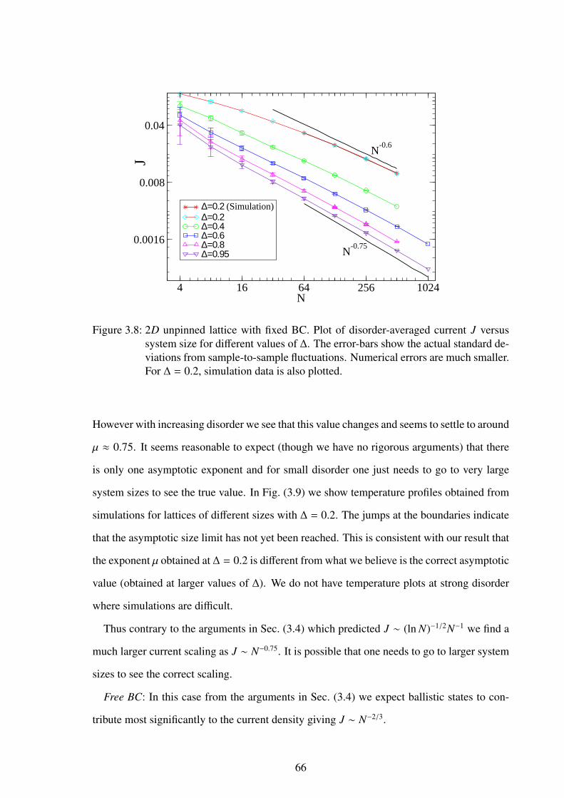
4 16 64 256 1024N
0.0016
0.008
0.04J
∆=0.2 (Simulation)∆=0.2∆=0.4∆=0.6∆=0.8∆=0.95
N-0.6
N-0.75
Figure 3.8: 2D unpinned lattice with fixed BC. Plot of disorder-averaged current J versussystem size for different values of ∆. The error-bars show the actual standard de-viations from sample-to-sample fluctuations. Numerical errors are much smaller.For ∆ = 0.2, simulation data is also plotted.
However with increasing disorder we see that this value changes and seems to settle to around
µ ≈ 0.75. It seems reasonable to expect (though we have no rigorous arguments) that there
is only one asymptotic exponent and for small disorder one just needs to go to very large
system sizes to see the true value. In Fig. (3.9) we show temperature profiles obtained from
simulations for lattices of different sizes with ∆ = 0.2. The jumps at the boundaries indicate
that the asymptotic size limit has not yet been reached. This is consistent with our result that
the exponent µ obtained at ∆ = 0.2 is different from what we believe is the correct asymptotic
value (obtained at larger values of ∆). We do not have temperature plots at strong disorder
where simulations are difficult.
Thus contrary to the arguments in Sec. (3.4) which predicted J ∼ (ln N)−1/2N−1 we find a
much larger current scaling as J ∼ N−0.75. It is possible that one needs to go to larger system
sizes to see the correct scaling.
Free BC: In this case from the arguments in Sec. (3.4) we expect ballistic states to con-
tribute most significantly to the current density giving J ∼ N−2/3.
66

0 0.2 0.4 0.6 0.8 1i/N
1
1.2
1.4
1.6
1.8
2
[Ti]
N=16N=32N=64N=128N=256
Figure 3.9: 2D unpinned case with fixed BC for ∆ = 0.2. Plot of disorder-averaged temper-ature profile [Ti] for different system sizes obtained from simulations.
In Figs. (3.10,3.11) we plot the disorder averaged transmission coefficient for ∆ = 0.8 and
∆ = 0.2 for different system sizes. Qualitatively these results look very similar to those for
fixed boundaries. However transmission is now significantly larger in the region of extended
states. The behaviour at frequencies ω → 0 is also different and we now find T (ω) ∼ ω in
contrast to T (ω) ∼ ω3 for fixed boundaries. From the plots of IPRs in Fig. (3.10) we note
that there is not much qualitative difference with the fixed boundary plots except in the low
frequency region.
The system size dependence of the disorder averaged current J for two different values of
∆ is shown in Fig. (3.12). For ∆ = 0.2 we get an exponent µ ≈ 0.5 while for the stronger
disorder case ∆ = 0.8 we see a different exponent µ ≈ 0.6. Again we believe that the strong
disorder value of µ = 0.6 is closer to the value of the true asymptotic exponent. This value is
close to the expected µ = 2/3 for free BC and significantly different from the value obtained
for fixed BC (µ ≈ 0.75). Thus the dependence of the value of µ on boundary conditions
exists even in the 2D case.
67

0 0.5 1 1.5 2ω
0
0.04
0.08
0.12
0.16T(
ω) 3 4 5 6
0
0.002
0.004
0.006
L=16L=32∆=0.8
n1
n2
n1
n2
0
0.0005
0.001
0.0015
0.002
0.0025
0 10 20 30 40 50 60 70 0 10
20 30
40 50
60 70
0
0.0005
0.001
0.0015
0.002
0.0025
0
0.5
1
1.5
2
2.5
3
0 10 20 30 40 50 60 70 0 10
20 30
40 50
60 70
0
0.5
1
1.5
2
2.5
3
x x
P−1
0.0001
0.001
0.01
0.1
1
0 1 2 3 4 5 6
1 10
100 1000
0 0.4 0.8 1.2 1.6
ωp
Figure 3.10: 2D unpinned case with free BC for ∆ = 0.8. TOP: Plot of the disorder averagedtransmission T (ω) versus ω. The various curves (from top to bottom) corre-spond to square lattices with N = 16, 32, 64, 128, 256, 512 respectively. We seethat transmission takes place in a small band ≈ (0−2) of the full range ≈ (0−6)of normal modes and, as can be seen in the inset, is negligible elsewhere. BOT-TOM: Plot shows the IPR (P−1) as a function of normal mode-frequency ωp.The curves are for N = 16 (blue), 32 (green) and 64 (red). In the inset we plotN2P−1 and the collapse at low frequencies shows that low frequency modes areextended. Also shown are two typical normal modes for one small (left) andone large value of P−1 for N = 64.
68
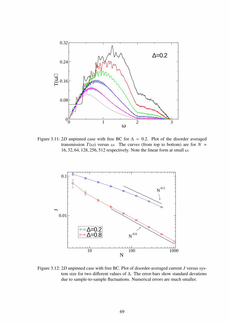
0 1 2 3ω
0
0.08
0.16
0.24
0.32
T(ω
)∆=0.2
Figure 3.11: 2D unpinned case with free BC for ∆ = 0.2. Plot of the disorder averagedtransmission T (ω) versus ω. The curves (from top to bottom) are for N =16, 32, 64, 128, 256, 512 respectively. Note the linear form at small ω.
10 100 1000N
0.01
0.1
J
∆=0.2∆=0.8
N-0.5
N-0.6
Figure 3.12: 2D unpinned case with free BC. Plot of disorder-averaged current J versus sys-tem size for two different values of ∆. The error-bars show standard devationsdue to sample-to-sample fluctuations. Numerical errors are much smaller.
69
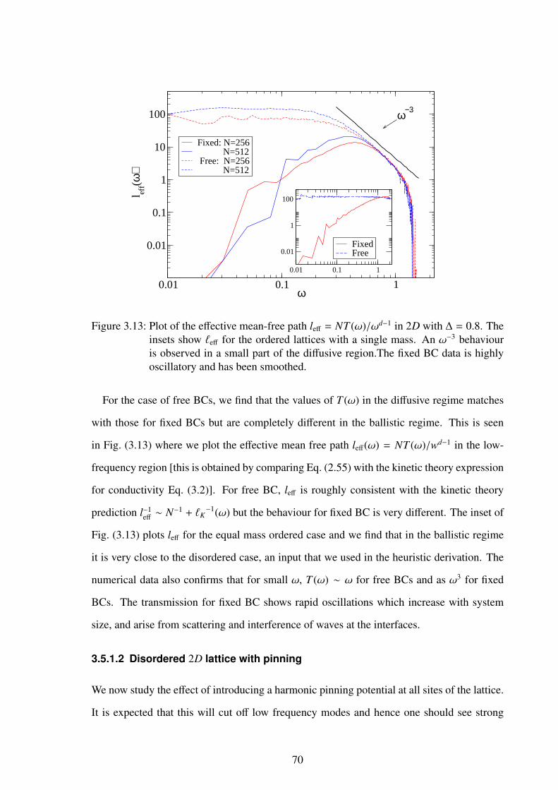
0.01 0.1 1ω
0.01
0.1
1
10
100
l eff(ω
)Fixed: N=256 N=512 Free: N=256 N=512
0.01 0.1 1
0.01
1
100
FixedFree
ω−3
Figure 3.13: Plot of the effective mean-free path leff = NT (ω)/ωd−1 in 2D with ∆ = 0.8. Theinsets show `eff for the ordered lattices with a single mass. An ω−3 behaviouris observed in a small part of the diffusive region.The fixed BC data is highlyoscillatory and has been smoothed.
For the case of free BCs, we find that the values of T (ω) in the diffusive regime matches
with those for fixed BCs but are completely different in the ballistic regime. This is seen
in Fig. (3.13) where we plot the effective mean free path leff(ω) = NT (ω)/wd−1 in the low-
frequency region [this is obtained by comparing Eq. (2.55) with the kinetic theory expression
for conductivity Eq. (3.2)]. For free BC, leff is roughly consistent with the kinetic theory
prediction l−1eff ∼ N−1 + `K
−1(ω) but the behaviour for fixed BC is very different. The inset of
Fig. (3.13) plots leff for the equal mass ordered case and we find that in the ballistic regime
it is very close to the disordered case, an input that we used in the heuristic derivation. The
numerical data also confirms that for small ω, T (ω) ∼ ω for free BCs and as ω3 for fixed
BCs. The transmission for fixed BC shows rapid oscillations which increase with system
size, and arise from scattering and interference of waves at the interfaces.
3.5.1.2 Disordered 2D lattice with pinning
We now study the effect of introducing a harmonic pinning potential at all sites of the lattice.
It is expected that this will cut off low frequency modes and hence one should see strong
70

n1
n2n1
n2
0 0.005 0.01 0.015 0.02 0.025 0.03 0.035 0.04
0 10 20 30 40 50 60 70 0 10
20 30
40 50
60 70
0 0.005
0.01 0.015
0.02 0.025
0.03 0.035
0.04
0 0.05 0.1 0.15 0.2 0.25 0.3 0.35 0.4 0.45 0.5
0 10 20 30 40 50 60 70 0 10
20 30
40 50
60 70
0 0.05
0.1 0.15
0.2 0.25
0.3 0.35
0.4 0.45
0.5
x x
P−1
0.001
0.01
0.1
1
2.5 3 3.5 4 4.5 5 5.5ωp
2.5 3 3.5 4 4.5 5 5.5ω
1e-05
0.0001
0.001
0.01T
(ω)
Figure 3.14: 2D pinned case for ∆ = 0.4 and ko = 10.0. TOP: Plot of the disorder averagedtransmission T (ω) versus ω. The various curves (from top to bottom) corre-spond to lattices with N = 16, 32, 64 respectively. Here we choose γ =
√10.
BOTTOM: Plot of the IPR (P−1) as a function of normal mode-frequency ωp.The curves are for N = 16 (blue), 32 (green) and 64 (red). Also shown are twotypical normal modes for one small (left) and one large value of P−1 for N = 64.
71

1 1.5 2 2.5 3 3.5 4ω
1e-05
0.0001
0.001
0.01
0.1
T(ω
)
Figure 3.15: 2D pinned case for ∆ = 0.4 and ko = 2.0. Plot of the disorder averagedtransmission T (ω) versus ω . The various curves (from top to bottom) are forN = 16, 32, 64, 128, 256, 512 respectively. Here we choose γ =
√2.
localization effects. The localization length ` will decrease both with increasing ∆ and in-
creasing ko (in 1D, heuristic arguments give ` ∼ 1/(∆2ko) [21]). In Figs. (3.14,3.15) we plot
the transmission coefficients for two cases with on-site potentials ko = 10.0 and ko = 2.0
respectively, and ∆ = 0.4. We also plot the IPR in Fig. (3.14). Unlike in the unpinned case
we now find that the transmission coefficients are much smaller and fall more rapidly with
system size.
From the plot of P−1 we find that for all the modes, the value of P−1 does not change
much with system size which implies that all modes are localized. The allowed frequency
bands correspond to the transmission bands. The two wavefunctions plotted in Fig. (3.14)
correspond to one relatively small and one large P−1 value and clearly show that both states
are localized.
The system size dependence of the integrated current is shown in Fig. (3.16) for the two
parameter sets. The values of µ ≈ 1.6, 3.65 for the two sets indicate that at large enough
length scales one will get a current falling exponentially with system size and hence we
72
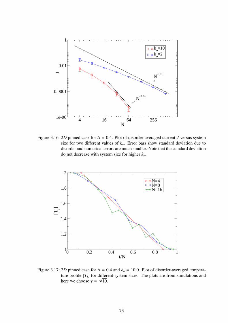
4 16 64 256N
1e-06
0.0001
0.01
1
J
ko=10
ko=2
N-1.6
N-3.65
Figure 3.16: 2D pinned case for ∆ = 0.4. Plot of disorder-averaged current J versus systemsize for two different values of ko. Error bars show standard deviation due todisorder and numerical errors are much smaller. Note that the standard deviationdo not decrease with system size for higher ko.
0 0.2 0.4 0.6 0.8 1i/N
1
1.2
1.4
1.6
1.8
2
[Ti]
N=4N=8N=16
Figure 3.17: 2D pinned case for ∆ = 0.4 and ko = 10.0. Plot of disorder-averaged tempera-ture profile [Ti] for different system sizes. The plots are from simulations andhere we choose γ =
√10.
73

have an insulating phase. In Fig. (3.17) we plot the temperature profiles for the set with
∆ = 0.4, ko = 10.0 . In this case it is difficult to obtain steady state temperature profiles from
simulations for larger system sizes. The reason is that the temperature (unlike current) gets
contributions from all modes (both localized and extended) and equilibrating the localized
modes takes a long time.
3.5.2 Results in three dimensions
In this section we mostly consider N × N × N lattices with periodic boundary conditions in
the ν = 2, 3 directions. Some results for N × N2 × N3 lattices with N2 = N3 < N will also
be described. Preliminary results for the case of free BCs are given and indicate that there
is no dependence of the exponent µ on BCs. It is not clear to us whether this is related to
the boundedness of the fluctuations in xn and the decay of the correlations between xn and xl
(like |n − l|−1) in d = 3 and their growth (with N) in d < 3.
3.5.2.1 Disordered 3D lattice without pinning
Fixed BC: we have used both the numerical approach and simulations for sizes up to 32 ×
32×32 for which we have data for T (ω). For larger systems the matrices become too big and
we have not been able to use the numerical approach. Hence, for larger system sizes we have
only performed simulations, including some on N × N2 × N2 lattices. For these cases only
the current J is obtained. The number of averages varies from over 100 samples for N = 16
to two samples for N = 64. In Figs. (3.18,3.19) we plot the disorder averaged transmission
coefficient for two different disorder strengths, ∆ = 0.8 and ∆ = 0.2, for different system
sizes. The corresponding plots of IPRs as a function of normal mode frequency ωp, for
single disorder realizations, are also given. From the IPR plots we get an idea of the typical
range of allowed normal mode frequencies and their degree of localization. Low IPR values
which scale as N−3 imply extended states while large IPR values which do not change much
with system size denote localized states.
From Figs. (3.18,3.19) we make the following observations.
74

0 1 2 3 4 5 6 7 8ω
0
0.4
0.8
N T
(ω)
N=8N=16N=32
0 1 2 3 4 5 6 7 80
0.04
0.08T(
ω)
N=8N=16N=32
(i)
(ii)
P−
1P
−1
N3
ωp
0.0001
0.001
0.01
0.1
1
0 1 2 3 4 5 6 7 8
1
10
100
1000
10000
0 1 2 3 4 5 6 7 8
Figure 3.18: 3D unpinned case with fixed BC for ∆ = 0.8. TOP: Plot of the disorder averagedtransmission T (ω) versus ω. The inset shows the same data multiplied by afactor of N. BOTTOM: Plot of the IPR (P−1) and scaled IPR (N3P−1) as afunction of normal mode-frequency ωp for a fixed disorder-realization. Thecurves are for N = 8 (green) and 16 (red).
75

0 1 2 3 4ω
0
0.12
0.24
0.36T
(ω)
N = 8N = 16N = 32
P−1
P−1
N3
ωp
0.01
0.1
1
10
0 0.5 1 1.5 2 2.5 3 3.5 4
1
10
100
0 0.5 1 1.5 2 2.5 3 3.5 4
Figure 3.19: 3D unpinned case with fixed BC for ∆ = 0.2. TOP: Plot of the disorder averagedtransmission T (ω) versus ω. The uppermost curve is the transmission curve forthe binary mass ordered lattice for N = 16. BOTTOM: Plot of IPR (P−1)and scaled IPR (N3P−1) as a function of normal mode-frequency ωp for a fixeddisorder realization. The curves are for N = 8 (green) and 16 (red).
76
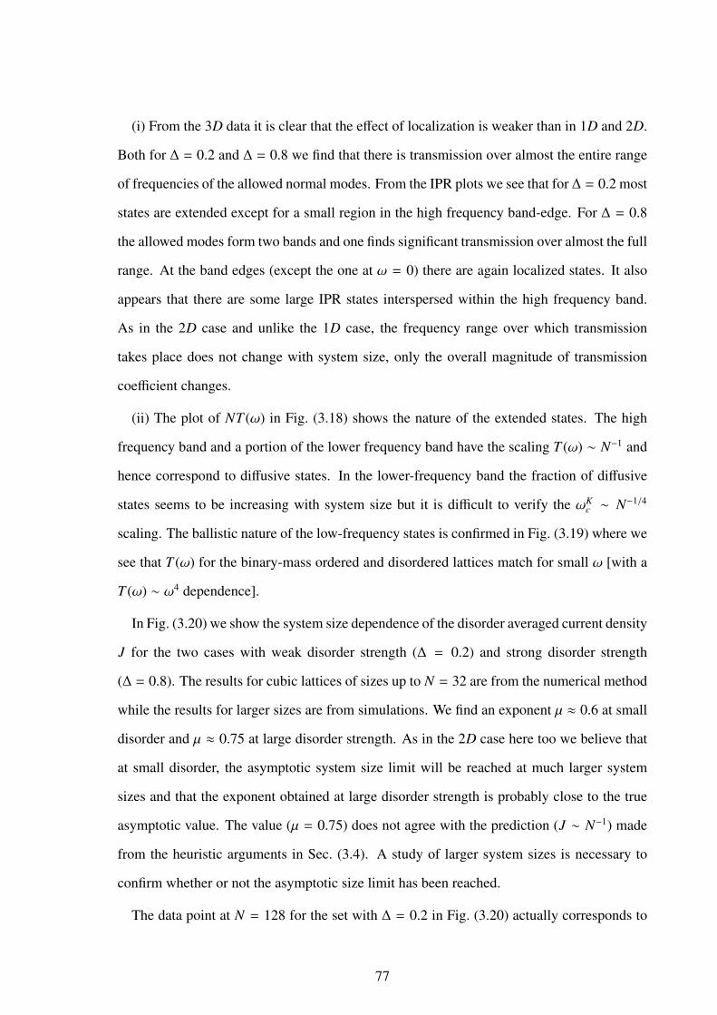
(i) From the 3D data it is clear that the effect of localization is weaker than in 1D and 2D.
Both for ∆ = 0.2 and ∆ = 0.8 we find that there is transmission over almost the entire range
of frequencies of the allowed normal modes. From the IPR plots we see that for ∆ = 0.2 most
states are extended except for a small region in the high frequency band-edge. For ∆ = 0.8
the allowed modes form two bands and one finds significant transmission over almost the full
range. At the band edges (except the one at ω = 0) there are again localized states. It also
appears that there are some large IPR states interspersed within the high frequency band.
As in the 2D case and unlike the 1D case, the frequency range over which transmission
takes place does not change with system size, only the overall magnitude of transmission
coefficient changes.
(ii) The plot of NT (ω) in Fig. (3.18) shows the nature of the extended states. The high
frequency band and a portion of the lower frequency band have the scaling T (ω) ∼ N−1 and
hence correspond to diffusive states. In the lower-frequency band the fraction of diffusive
states seems to be increasing with system size but it is difficult to verify the ωKc ∼ N−1/4
scaling. The ballistic nature of the low-frequency states is confirmed in Fig. (3.19) where we
see that T (ω) for the binary-mass ordered and disordered lattices match for small ω [with a
T (ω) ∼ ω4 dependence].
In Fig. (3.20) we show the system size dependence of the disorder averaged current density
J for the two cases with weak disorder strength (∆ = 0.2) and strong disorder strength
(∆ = 0.8). The results for cubic lattices of sizes up to N = 32 are from the numerical method
while the results for larger sizes are from simulations. We find an exponent µ ≈ 0.6 at small
disorder and µ ≈ 0.75 at large disorder strength. As in the 2D case here too we believe that
at small disorder, the asymptotic system size limit will be reached at much larger system
sizes and that the exponent obtained at large disorder strength is probably close to the true
asymptotic value. The value (µ = 0.75) does not agree with the prediction (J ∼ N−1) made
from the heuristic arguments in Sec. (3.4). A study of larger system sizes is necessary to
confirm whether or not the asymptotic size limit has been reached.
The data point at N = 128 for the set with ∆ = 0.2 in Fig. (3.20) actually corresponds to
77

8 16 32 64 128N
0.01
0.1
J
∆ = 0.2 ∆ = 0.2 (Free BC)∆ = 0.8 ∆ = 0.8 (Free BC)
N-0.75
N-0.57
N-0.71
Figure 3.20: 3D unpinned case with fixed and free BCs. Plot of disorder-averaged currentJ versus system size for two different values of ∆. The data for ∆ = 0.2 isfrom simulations. The error-bars show standard deviations due to disorder andnumerical errors are smaller.
a lattice of dimensions 128 × 48 × 48 and we believe that the current value is very close to
the expected fully 3D value. To see this point, we have plotted in Fig. (3.21) results from
nonequilibrium simulations with N × N2 × N2 lattices with N2 ≤ N.
Finally, in Fig. (3.22) we show temperature profiles (for single disorder realizations) ob-
tained from simulations for lattices of different sizes and with ∆ = 0.2. The jumps at the
boundaries again indicate that the asymptotic system size limit has not been reached even at
the largest size.
Free BC: In this case from the arguments in Sec. (3.4) we expect ballistic states to con-
tribute most significantly to the current density giving J ∼ N−3/4.
In Fig. (3.23) we plot the disorder averaged transmission coefficient for ∆ = 0.8 for dif-
ferent system sizes. The transmission function is very close to that for the fixed boundary
case except in the frequency region corresponding to non-diffusive states. At ω→ 0 we now
expect, though it is hard to verify from the data, that T (ω) ∼ ω2 in contrast to T (ω) ∼ ω4 for
78

0 0.2 0.4 0.6 0.8 1N
2/N
0
0.01
0.02
0.03
0.04
0.05
[J]
N = 8N = 16N = 32N = 64N = 128
Figure 3.21: 3D unpinned case with fixed BC for ∆ = 0.2. Plot of disorder-averaged currentdensity J (with the definition J = I/N2
2 ) versus N2/N for different fixed valuesof N. We see that the 3D limiting value is reached at quite small values of N2/N.
fixed boundaries.
The system size dependence of the disorder averaged current J for two different values of
∆ is shown in Fig. (3.20). We find that the current values are quite close to the fixed BC case
and the exponent obtained at the largest system size studied for this case is µ ≈ 0.71. This
value is close to the expected µ = 3/4 for free BC.
We now compare the transmission coefficient for free and fixed BCs in the ballis-
tic regime. This is plotted in Fig. (3.24) where we show the effective mean free path
leff(ω) = NT (ω)/wd−1 in the low-frequency region. As in the 2D case we again find that
for free BCs, leff is roughly consistent with the kinetic theory prediction l−1eff ∼ N−1 + `K
−1(ω)
and the behaviour for fixed BCs is very different. The inset of Fig. (3.24) plots leff for the
equal mass ordered case and we find that in the ballistic regime it is very close to the dis-
ordered case. The numerical data confirms the input in our theory on the form of T (ω) for
small ω, i.e. T (ω) ∼ ω2 for free BCs and as ω4 for fixed BCs. The transmission for fixed
BC shows rapid oscillations which increase with system size, and arise from scattering and
79

0 0.2 0.4 0.6 0.8 1i/N
1
1.2
1.4
1.6
1.8
2
[Ti]
N=8N=16N=32N=64N=128
Figure 3.22: 3D unpinned case with fixed BC for ∆ = 0.2. Plot of temperature profile Ti
in a single disorder realization for different system sizes. The plots are fromsimulations.
0 2 4 6 8ω
0
0.02
0.04
0.06
0.08
0.1
T(ω
)
0 2 4 6 8ω
0
0.4
0.8
1.2
1.6
NT
(ω)
N = 8N = 16N = 32
Figure 3.23: 3D unpinned case with free BC for ∆ = 0.8. Plot of the disorder averagedtransmission T (ω) versus ω. The inset shows the same data multiplied by afactor of N.
80
0.1 1ω
0.01
0.1
1
10
l eff(ω
)Fixed: N=256 N=512Free: N=16 N=32
0.1 1
0.01
0.1
1
10
FixedFree
ω−4
Figure 3.24: Plot of the effective mean-free path leff = NT (ω)/ωd−1 in 3D with ∆ = 0.8 forfixed and free BCs. The insets show `eff for the ordered system with a singlemass. An ω−4 behaviour is observed in a small part of the diffusive region.Thefixed BC data is highly oscillatory and has been smoothed.
interference of waves at the interfaces.
3.5.2.2 Disordered 3D lattice with pinning
For the pinned case, we again use both the numerical method and simulations for sizes up to
N = 32. For N = 64 only nonequilibrium simulation results are reported.
In Figs. (3.25,3.26) we plot the disorder averaged transmission coefficient for ∆ = 0.2 and
∆ = 0.8 with ko = 10.0. The corresponding IPRs P−1 and scaled IPRs N3P−1 are also shown.
From the IPR plots we notice that the spectrum of the 3D disordered pinned chain has
a similar interesting structure as in the 2D case with two bands and a gap which is seen at
strong disorder. However unlike the 2D case where all states were localized, here the IPR
data indicates that most states except those at the band edges are diffusive. We see localized
states at the band edges and also there seem to be some localized states interspersed among
the extended states within the bands. The insets in Figs. (3.25,3.26) show that there is a
reasonable N−1 scaling of the transmission data in most of the transmitting region. This is
clearer at larger system sizes. Thus, unlike the unpinned case where low frequency extended
81

3 4 5ω
0
0.2
0.4
0.6
0.8
N T
(ω)
3 3.5 4 4.5 5ω
0
0.02
0.04
0.06
0.08
0.1T
( ω)
N = 8N = 16N = 32
−1
P−
1P
N3
ωp
0.001
0.01
0.1
3 3.5 4 4.5 5 5.5
1
10
100
1000
3 3.5 4 4.5 5 5.5
Figure 3.25: 3D pinned case for ∆ = 0.2 and ko = 10.0. TOP: Plot of the disorder averagedtransmission T (ω) versus ω. BOTTOM: Plot of the IPR (P−1) and scaled IPR(N3P−1) as a function of normal mode-frequency ωp. The curves are for N = 8(green) and 16 (red).
82

−1
P−
1P
N3
ωp
1
10
100
1000
10000
2 3 4 5 6 7 8 9 10 11
0.001
0.01
0.1
1
2 3 4 5 6 7 8 9 10 11
2 3 4 5 6 7 8 9 10 11ω
0
0.008
0.016
0.024
0.032
0.04T
(ω)
N=8N=16N=32
2 4 6 8 10ω0
0.1
0.2
0.3
N T
(ω)
Figure 3.26: 3D pinned case for ∆ = 0.8 and ko = 10.0. TOP: Plot of the disorder averagedtransmission T (ω) versus ω. BOTTOM: Plot of the IPR (P−1) and scaled IPR(N3P−1) as a function of normal mode-frequency ωp. The curves are for N = 8(green) and 16 (red).
83

8 16 32 64 128N
0.001
0.01
0.1
J
∆=0.2 ; ko=1.0
∆=0.2 ; ko=5.0
∆=0.2 ; ko=10.0
∆=0.8 ; ko=10.0
N-1
Figure 3.27: 3D pinned case. Plot of disorder-averaged current J versus system size fordifferent values of ko and ∆. The data sets for ∆ = 0.2 for different values of ko
are from simulations while the data for ∆ = 0.8 is from numerics.
states were ballistic or super-diffusive, here we find that there is no transmittance at small
(ω→ 0) frequencies and that all states are diffusive.
From the above discussion we expect Fourier’s law to be valid in the 3D pinned disordered
lattice. The system size dependence of the disorder averaged current J for different disorder
strengths is plotted in Fig. (3.27). For all the parameter sets the exponent obtained is close to
µ = 1 corresponding to a finite conductivity and validity of Fourier’s law. The temperature
profiles plotted in Fig. (3.28) have small boundary temperature jumps and indicate that the
asymptotic size limit has already been reached.
One might expect that at very strong disorder, all states should become localized and then
one should get a heat insulator. The parameter set corresponding to Fig. (3.26) corresponds
to strong disorder and for this we still find a significant fraction of extended states. Thus
for the binary mass case it appears that there are always extended states. We have some
results for the case with a continuous mass distribution ( masses are chosen from a uniform
distribution between 1−∆ and 1+∆). In this case we find that the effect of disorder is stronger
84

0 0.2 0.4 0.6 0.8 1i/N
1
1.2
1.4
1.6
1.8
2
[Ti]
N=8N=16N=32N=64
Figure 3.28: 3D pinned case for ∆ = 0.2 and ko = 10.0. Plot of temperature profile Ti
in a single disorder realization for different system sizes. The plots are fromsimulations.
and the transmission at all frequencies is much reduced compared to the binary mass case.
However we cannot see the exponential decrease in transmission with system size and so it
is not clear if an insulating behaviour is obtained. Further numerical studies are necessary to
understand the asymptotic behaviour.
3.6 Conclusions
We have studied heat conduction in isotopically disordered harmonic lattices with scalar dis-
placements in two and three dimensions. The main question addressed is the system size
dependence of the heat current, which is computed using Green’s function based numerical
methods as well as nonequilibrium simulations. We have tried to understand the size de-
pendence by looking at the phonon transmission function T (ω) and examining the nature of
the energy transport in different frequency regimes. We also described a heuristic analytical
calculation based on localization theory and kinetic theory and compared their predictions
with our numerical and simulation results. This comparison is summarized in Table (3.1).
85

d = 2 d = 3
Analytical Numerical Analytical Numerical
Pinned exp (−bN) N−3.7 N−1 N−1.0
Fixed N−1(ln N)−1/2 N−0.75 N−1 N−0.75
Free N−2/3 N−0.6 N−3/4 N−0.71
Table 3.1: The table summarizes the main results. The numerical (and nonequilibrium sim-ulation) results obtained are compared, in two and three dimensions, with theanalytical predictions obtained from our heuristic arguments. The error bar forthe numerically obtained exponent values is of the order ±0.02. This error is es-timated from the errors in the last few points of the J-versus-N data. NB: Thesystem sizes used may well be far from asymptotic.
The most interesting findings of this work are:
(i) For the unpinned system we find that in 2D there are a large number of localized modes
for which phonon transmission is negligible. In 3D the number of localized modes is much
smaller. The extended modes are either diffusive or ballistic. Our analytic arguments show
that the contribution of ballistic modes to conduction is dependent on BCs and is strongly
suppressed for the case of fixed BCs, the more realistic case. In 3D this leads to diffusive
modes dominating for large system sizes and Fourier’s law is satisfied. Thus a finite heat
conductivity is obtained for the 3D disordered harmonic crystal without the need of invoking
anharmonicity as is usually believed to be necessary [77, 2]. This is similar to what one
obtains when one adds stochasticity to the time evolution in the bulk as shown by [83]. Our
numerical results verify the predictions for free BCs and we believe that much larger system
sizes are necessary to verify the fixed BC results ( this is also the case in 1D [19, 22]).
(ii) In two dimensions the pinned disordered lattice shows clear evidence of localization and
we obtain a heat insulator with exponential decay of current with system size.
(iii) Our result for the 3D pinned disordered lattice provides the first microscopic verification
of Fourier’s law in a three dimensional system. For the binary mass distribution we do not
see a transition to insulating behaviour with increasing disorder. For a continuous mass
distribution we find that the current is much smaller (than the binary mass case with the
same value of ∆) but it is not clear whether all states get localized and if an insulating phase
86
exists.
3.7 appendix
Kinetic theory: Kinetic theory becomes valid in the limit of small disorder. Its basic object
is the Wigner function, f , which describes the phonon density in phase space and is governed
by the transport equation
∂
∂tf (r, k, t) + ∇ω(k) · ∇r f (r, k, t) = C f (r, k, t) . (3.19)
Here r ∈ Rd (boundary conditions could be imposed), k ∈ [−π, π]d is the wave number of the
first Brioullin zone, ω is the dispersion relation of the constant mass harmonic crystal, and C
is the collision operator. It acts only on wave numbers and is given by
C f (k) = (2π)−d+1ω(k)2∆2∫
[−π,π]ddk′
δ(ω(k) − ω(k′)
)(f (k′) − f (k)
). (3.20)
We refer to [6] for a derivation. In the range of validity of (3.19), (3.20) we can think of
phonons as classical particles with energy ω and velocity ∇ω(k). They are scattered by the
impurities from k to dk′ with the rate
(2π)−d+1ω(k)2∆2δ(ω(k) − ω(k′)
)dk′. (3.21)
Collisions are elastic. We distinguish the following cases
(i) no pinning potential. Here for small k one has ω(k) = |k| and |∇ω(k)| = 1. From (3.20)
the total scattering rate behaves as |k|d+1. This is the basis for the discussion in connection
with Eq. (3.2).
(ii) pinning potential. In this case ω(k) = ω0 + k2 for small k. The prefactor in (3.20) can
be replaced by ω20. The velocity is k and the scattering is isotropic with rate |k|d−2. Thus the
diffusion coefficient results as D(k) |k|−d+4 which vanishes as |k| → 0 for d = 2, 3. Hence
there is no contribution to the thermal conductivity from the small k modes.
87

4 Green-Kubo formula for opensystems
The Green-Kubo formula [84, 85] is a cornerstone of the study of transport phenomena. In
sec. (1.1.3) we saw that for a system governed by Hamiltonian dynamics, the currents that
flow in response to small applied fields can be related to the equilibrium correlation functions
of the currents. For the case of heat transport the Green-Kubo formula (in the classical limit)
gives:
κ =1
KBT 2 limε→0
∫ ∞
0dte−εt lim
L→∞
1L〈JE(t)JE(0)〉, (4.1)
where κ is the thermal conductivity of a system of linear dimension L at temperature T . For
a d-dimensional system this formula can be written as:
κ =1
KBT 2 limε→0
∫ ∞
0dte−εt lim
L→∞
1Ld 〈JE(t)JE(0)〉. (4.2)
The autocorrelation function on the right hand side is evaluated in equilibrium, without a
temperature gradient. Since in this chapter we will be talking about heat current JE only,
for the rest of the chapter we denote it by J. The total heat current in the system is J(t) =∫j(x, t)dx, where j(x, t) is the heat flux density. The order of the limits in Eq. (4.2) is
important. With the correct order of limits, one can calculate the correlation functions with
arbitrary boundary conditions and apply Eq. (4.2) to obtain the response of an open system
with reservoirs at the ends. There have been a number of derivations of Eq. (4.2) by various
authors [84, 85, 86]. In the introduction of this thesis we have presented one such derivation.
There are several situations where the Green-Kubo formula in Eq. (4.2) is not applicable.
For example, for the small structures that are studied in mesoscopic physics, the thermo-
88

dynamic limit is meaningless, and one is interested in the conductance of a specific finite
system. Secondly, in many low dimensional systems, heat transport is anomalous and the
thermal conductivity diverges [59]. In such cases it is impossible to take the limits as in
Eq. (4.2); one is there interested in the thermal conductance as a function of L instead of
an L-independent thermal conductivity. The usual procedure that has been followed in the
heat conduction literature is to put a cut-off at tc ∼ L, in the upper limit in the Green-Kubo
integral [59]. There is no rigorous justification of this assumption. A related case is that of
integrable systems, where the infinite time limit of the correlation function in Eq. (4.2) is
non-zero. Another way of using the Green-Kubo formula for finite systems is to include the
infinite reservoirs also while applying the formula and this was done, for example, by Allen
and Ford [87] for heat transport and by Fisher and Lee [88] for electron transport. Both these
cases are for non-interacting systems and the final expression for conductance is what one
also obtains from the nonequilibrium Green’s function approach, a formalism of transport
commonly used in the mesoscopic literature. More recently, it has been shown that Green-
Kubo like expressions for finite open systems can be derived rigorously by using the steady
state fluctuation theorem (SSFT) [89, 90, 91, 92].
There are mainly two parts of this chapter. In this first part of this chapter, we derive a
Green-Kubo like formula for open systems, without invoking the SSFT. Our proof applies to
all classical systems, of arbitrary size and dimensionality, with a variety of commonly used
implementations of heat baths. The proof consists in first solving the equation of motion
for the phase space probability distribution to find the O(∆T ) correction to the equilibrium
distribution function. The average current at this order can then be expressed in terms of the
equilibrium correlation 〈J(t)J f p(0)〉, where J f p is a specified current operator. Secondly we
use the energy continuity equations to relate two different current-current correlation func-
tions, namely 〈J(0)J(t)〉 and 〈J(0)Jb(t)〉 where Jb is an instantaneous current operator involv-
ing heat flux from the baths. Finally one relates 〈J(0)Jb(t)〉 to 〈J(0)J f p(t)〉 and then, using
time-reversal invariance, to 〈J(t)J f p(0)〉. For baths with stochastic dynamics, time-reversal
invariance follows from the detailed balance principle, which is an essential requirement of
89

our proof.
In the second part we obtain an exact expression for the time auto-correlation function for
heat current in the NESS for a mass disordered harmonic chain of arbitrary length, expressed
in terms of the non-equilibrium Green’s functions. We show that it satisfies the GK formula
derived in the first section. Using this correlation function we also calculate the asymptotic
system size scaling of fluctuations in current in NESS.
The entire chapter is organised as follows. In Sec. (4.1) we present our proof of the formula
for 1D lattice model in detail and outline the proof for other baths in Sec. (4.2). In Sec. (4.3)
we extend our proof for higher dimensional lattice models. We also prove this formula for
fluid system coupled to Maxwell baths in Sec. (4.4). Finally in Sec. (4.5) we present the
calculation of time autocorrelation function and prove that it also satisfies a similar open
system formula.
4.1 Proof of the formula for 1D lattice model
We first give a proof of our linear response result for a 1D lattice model with white noise
Langevin baths. We consider the following general Hamiltonian:
H =N∑
l=1
[mlv2
l
2+ V(xl)
]+
N−1∑l=1
U(xl − xl+1) , (4.3)
where x = xl, v = vl with l = 1, 2...N denotes displacements of the particles about their
equilibrium positions and their velocities, and ml denotes their masses. The particles at the
ends are connected to two white noise heat baths of temperatures TL and TR respectively.
The equations of motion of the system are given by:
mlvl = fl − δl,1[γLv1 − ηL] − δl,N[γRvN − η
R ], (4.4)
where fl = −∂H/∂xl, and ηL,R(t) are Gaussian noise terms with zero mean and satisfying
the fluctuation dissipation relations: 〈ηL,R(t)ηL,R(t′)〉 = 2γL,RkBTL,Rδ(t − t′) . There are three
stages toward proving the open system GK formula.
First stage : In the first part of the proof we obtain an expression for the nonequilibrium
90

steady state average 〈J〉∆T , at linear order in ∆T , and then we relate this to the equilib-
rium correlation function 〈J(t)J(0)〉. The 〈...〉 denotes a thermal equilibrium average. Time-
dependent equilibrium correlation functions require an averaging both over initial conditions
as well as over paths. In the Fokker-Planck representation this can be obtained using the
time-evolution operator, while in the Langevin representation thermal noise occurs explic-
itly and has to be averaged over. Corresponding to the stochastic Langevin equations in
Eq. (4.4), one has a Fokker-Planck (FP) equation for the phase space distribution P(x, v, t).
Setting TL = T + ∆T/2 and TR = T − ∆T/2 we write the FP equation in the following form:
∂P(x, v, t)∂t
= LP(x, v, t) + L∆T P(x, v, t) , (4.5)
where L(x, v) = LH +∑l=1,N
γl
ml
∂
∂vl
(vl +
kBTml
∂
∂vl
)L∆T (v) =
kB∆T2
(γL
m21
∂2
∂v21
−γR
m2N
∂2
∂v2N
), (4.6)
where LH = −∑
l[ vl ∂/∂xl + ( fl/ml) ∂/∂vl ] is the Hamiltonian Liouville operator and
γ1 = γL, γN = γR. For ∆T = 0 the steady state solution of the FP equation is known and is
just the usual equilibrium Boltzmann distribution P0 = e−βH/Z, where Z =∫
dxdve−βH is the
canonical partition function [β = (kBT )−1]. It is easily verified that LP0 = 0. For ∆T , 0, we
solve Eq. (4.5) by perturbation theory, starting from the equilibrium solution at time t = −∞.
Writing P(x, v, t) = P0 + p(x, v, t), we obtain the following solution at O(∆T ):
p(x, v, t) =∫ t
−∞
dt′ eL(t−t′) L∆T P0(x, v) = ∆β∫ t
−∞
dt′ eL(t−t′) J f p(v) P0(x, v) ,
with J f p(v) = (∆β P0)−1L∆T P0 = −γL
2
[v2
1 −kBTm1
]+γR
2
[v2
N −kBTmN
]. (4.7)
To define the current operator, one first defines the local energy density at the lth site:
εl = mlv2l /2+V(xl)+ 1
2 [U(xl−1 − xl)+U(xl − xl+1)]. Taking a time derivative gives the energy
continuity equation
dεl/dt + jl+1,l − jl,l−1 = j1,L δl,1 + jN,R δl,N , (4.8)
91
where jl+1,l =12
(vl + vl+1) fl+1,l
gives the current from the lth to the l + 1th site ( fl+1,l is the force on l + 1th particle due to
lth particle). We define the total current flowing through the system as J =∑N−1
l=1 jl+1,l . The
expectation value of the total current is then given by:
〈J〉∆T =
∫dxdv J p(x, v)
= ∆β
∫ ∞
0dt
∫dxdv J eLt J f p P0
= ∆β
∫ ∞
0dt 〈J(t)J f p(0)〉 . (4.9)
Second stage : In this part we prove
〈J(t)J f p(0)〉 = −〈J(0)J f p(t)〉. (4.10)
Eq. (4.10) is a statement of time-reversal symmetry. To prove this we write 〈J f p(t)J(0)〉 =∫dq
∫dq′J f p(q)J(q′)P0(q′)W(q, t|q′, 0) where W(q, t|q′, 0) denotes the transition probabil-
ity from q′ = (x′, v′) to q = (x, v) in time t. Then, using the detailed balance principle,
W(x, v, t|x′, v′, 0)P0(x′, v′) = W(x′,−v′, t|x,−v, 0)P0(x,−v) (see [93, 94, 95]) and the fact
that J is odd in the velocities while J f p is even, one gets 〈J f p(t)J(0)〉 = −〈J f p(0)J(t)〉 as
follows.
〈J f p(t)J(0)〉T =
∫dq
∫dq′J f p(q)J(q′)P0(q′)W(q, t|q′, 0)
=
∫dq
∫dq′J f p(q′)J(q)P0(q)W(q′, t|q, 0)
=
∫dq
∫dq′J f p(q′)J(q)P0(x′,−v′)W(x,−v, t|x′,−v′, 0)
=
∫dq
∫dq′J f p(x′,−v′)J(x,−v)P0(q′)W(q, t|q′, 0)
= −〈J(t)J f p(0)〉T , (4.11)
where we have interchanged q and q′ in the second line and used detailed balance in the
third line. Finally in the fourth line we have reversed all the velocity variables and used
the fact that J(x, v) is odd under velocity reversal while J f p is not. The Eq. (4.10) can be
92
proved in a direct but equivalent way which is as follows: An integration by parts followed
by the transformation v→ −v yields: 〈J(t)J f p(0)〉 =∫
dxdvJeLtJ f pP0 =∫
dxdvJ f pP0e¯LtJ =
−∫
dxdvJ f pP0eL†tJ where T ¯L = L† = LH −∑
l=1,N [vl − (βml)−1∂vl](γl/ml)∂vl and T de-
notes time reversal. We now note the operator identities LP0 = P0L† and consequently
eLtP0 = P0eL†t which can be proved using the form of P0. Using this in the above equation
immediately gives: 〈J(t)J f p(0)〉 = −∫
dxdvJ f peLtJP0 = −〈J(0)J f p(t)〉. Using this relation
in Eq. (4.9) we get
〈J〉∆T =∆T
KBT 2
∫ ∞
0dt 〈J f p(t)J(0)〉 . (4.12)
Third stage : Here we prove the following relations∫ ∞
0dt〈J(t)J(0)〉 = (N − 1)
∫ ∞
0dt〈J(0)Jb(t)〉 . (4.13)
and 〈J(0)Jb(t)〉 = 〈J(0)J f p(t)〉 (4.14)
which together complete the proof. For this let us define the current variable Jb as the mean
of the instantaneous heat currents flowing into the system from the left reservoir and flowing
out of the system to the right reservoir. Thus we have
Jb(t) =12
( j1,L − jN,R) (4.15)
where j1,L(t) = −γLv21(t) + ηL(t)v1(t) ,
jN,R(t) = −γRv2N(t) + ηR(t)vN(t) . (4.16)
It is easy to note that 〈J(0)〉 = 0. Now we prove
〈J(0)ηL(t)v1(t)〉 = 〈J(0)ηR(t)vN(t)〉 = 0 . (4.17)
To prove this we use Novikov’s theorem [96] which says: if ηi be a set of arbitrary Gaussian
noise variables with 〈ηi(t)η j(t′)〉 = Ki j(t, t′) and H[η] be a functional of the noise variables,
then
< ηi(t)H[η] > =∑
j
∫〈ηi(t)η j(t′)〉
⟨ δH[η]δη j(t′)
⟩dt′ ,
93
where δH[η]/δη j(t′) represents a functional derivative of H[η] with respect to η. Using the
fact 〈J(0)〉 = 0 and Eq. (4.17) we get Eq. (4.14).
To prove Eq. (4.13) let us define Dl(t) =∑l
k=1 εk−∑N
k=l+1 εk for l = 1, 2, ...N−1. Then from
the continuity equation Eq. (4.8) one can show that
dDl/dt = −2 jl+1,l(t) + 2Jb(t) . (4.18)
We multiply this equation by J(0), take a steady state average, and integrate over time from
t = 0 to ∞. Since DlJ has an odd power of velocity, we get 〈Dl(0)J(0)〉 = 0. Also
〈Dl(∞)J(0)〉 = 〈Dl(∞)〉 〈J(0)〉 = 0, and using these we immediately get∫ ∞
0dt〈 jl+1,l(t)J(0)〉 =∫ ∞
0dt〈Jb(t)J(0)〉. Summing over all bonds thus proves Eq. (4.13). Now using Eq. (4.14) first
and then Eq. (4.13) we write Eq. (4.12) as :
〈J〉∆T =∆T
KBT 2
1N − 1
∫ ∞
0dt 〈J(t)J(0)〉 . (4.19)
Dividing both sides of the above equation by (N − 1) and defining the steady state current
per bond between the reservoir and the system as j = J/(N − 1) we write Eq.(4.19) as
〈 j〉∆T =∆T
kBT 2
∫ ∞
0dt〈 j(t) j(0)〉 . (4.20)
Finally the conductance is given by
G = lim∆T→0
〈 j〉∆T
∆T=
1kBT 2
∫ ∞
0dt〈 j(t) j(0)〉 . (4.21)
Except the proofs of Eq. (4.10) and Eq. (4.14), other parts of the proof are quite general
and independent of the heat baths used. Proofs of Eq. (4.10) and Eq. (4.14) depend on the
specific bath chosen. In the next section we extend the proof to the cases where the noises
from the baths are exponentially correlated in time and noises are obtained by coupling the
lattice Hamiltonian to a deterministic bath model. Later we also give the proof of this formula
for fluid systems.
94
4.2 One dimensional lattice with other baths
We outline the proof for two other models of baths coupled to the lattice Hamiltonian. These
are (i) the Nose-Hoover bath and (ii) a Langevin bath with exponentially correlated noise.
Nose-Hoover bath: In this case the equations of motion are:
mlvl = fl − δl,1ζLv1 − δl,NζRvN , (4.22)
where ζL,R are themselves dynamical variables satisfying the equations of motion:
ζL =1θL
(m1v2
1
kBTL− 1)
ζR =1θR
(mNv2
N
kBTR− 1)
For small ∆T , we then write an equation of motion for the extended distribution function
P(x, v, ζL, ζR, t). This has the same form as Eq. (4.5) but now with:
LT = LH +ζL
m1
∂
∂v1v1 −
1θL
∂
∂ζL
(m1v2
1
kBT− 1
)+ζR
mN
∂
∂vNvN −
1θR
∂
∂ζR
(mNv2
N
kBT− 1
)L∆T =
∆T2kBT 2
(m1v2
1
θL
∂
∂ζL−
mNv2N
θR
∂
∂ζR
). (4.23)
If TL = TR = T, it is easy to verify that the equilibrium phase space density is given by:
P0 = P0(x, v) exp[−1
2
(θLζ
2L
m1+θRζ
2R
mN
)], (4.24)
and we assume that there is convergence to this distribution. Acting with L∆T on this, we
then obtain:
J f p = −12
(v21ζL − v2
NζR) . (4.25)
On the other hand, since −ζLv1 is the force from the left reservoir on the first particle, hence
j1,L = −ζLv21 and similarly, jN,R = −ζRv2
R. Hence from the definition of Jb in Eq. (4.15),
we obtain J f p = −Jb. This gives Eq. (4.14) with a minus sign on the right hand side i.e.
〈J(0)Jb(t)〉 = −〈J(0)J f p(t)〉. Now proceeding as in the second stage of the proof we get
95

〈J(t)J f p(0)〉 = 〈J(0)J f p(t)〉 without the minus sign (as there in Eq. (4.10)). This can be seen
from Eqs.(4.22) and (4.23). Under time reversal (x, v, ζ)→ (x,−v,−ζ), and since J, J f p both
are odd under time reversal, there is no minus sign in Eq.(4.11). Rest of the proof is similar
to the previous case.
Exponentially correlated bath: A simple way of realizing exponentially correlated heat
baths is to consider the following set of equations of motion:
mivl = fl + δl,1yL + δl,NyR , (4.26)
where yL, yR satisfy the following equations of motion:
yL = −yL
νLγL − γLv1 + η
L
yR = −yR
νRγR − γRvN + η
R ,
where ηL,R are Gaussian white noise satisfying 〈ηL,R(t)ηL,R(t′)〉 = 2kBTL,R/νL,Rδ(t − t′). As-
suming that the baths are coupled to the system at time t = −∞, the solution of the above
equations is:
yL = −γL∫ t
−∞
dt′e−(t−t′)/(νLγL)v1(t′) + ξL(t)
yR = −γR∫ t
−∞
dt′e−(t−t′)/(νRγR)vN(t′) + ξR(t)
where ξL =
∫ t
−∞
dt′e−(t−t′)/(νLγL)ηL(t′)
ξR =
∫ t
−∞
dt′e−(t−t′)/(νRγR)ηR(t′) .
The noise variables ξL,R satisfy 〈ξL,R(t)ξL,R(t′)〉 = kBTL,RγL,Re−|t−t′ |/(νL,RγL,R) , and so we verify
that yL,R are of the required form of exponentially correlated baths.
In this case we write a Fokker-Planck equation for the probability distribution for
P(x, v, yL, yR) and the forms of LT and L∆T are given by:
LT = LH −yL
m1
∂
∂v1+ γLv1
∂
∂yL+
∂
∂yL
(yL
νLγL +kBTνL
∂
∂yL
)−
yR
mN
∂
∂vN+ γRvN
∂
∂yR+
∂
∂yR
(yR
νRγR +kBTνR
∂
∂yR
),
96

L∆T =kB∆T
2
(1νL
∂2
∂y2L
−1νR
∂2
∂y2R
). (4.27)
One can verify that the equilibrium distribution is, in this case, given by:
P0 = P0(x, v) exp[−
12
(y2
L
γL +y2
R
γR
)], (4.28)
while J f p is given by:
J f p =1
2νL
[y2
L
(γL)2 −kBTγL
]−
12νR
[y2
R
(γR)2 −kBTγR
]. (4.29)
Now using the equation
ddt
(y2
L
2γL
)= −
y2L
νL(γL)2 − yLv1 +yLη
L
γL , (4.30)
and the fact that 〈J(0)yL(t)ηL(t)〉T = 0, it follows that:∫ ∞
0dt
⟨J(0)
y2L(t)
νL(γL)2
⟩T= −
∫ ∞
0dt〈J(0)yL(t)v1(t)〉T ,
and a similar result for the right reservoir. From the equations of motion Eq. (4.26), we get
j1,L = yLv1, jN,R = yRvN . Hence from the above equation and from the definitions of Jb in
Eq. (4.15), and of J f p in Eq. (4.29), we again get 〈J(0)J f p(t)〉T = 〈J(0)Jb(t)〉T . The other
steps of the proof are the same as for the white-noise case.
4.3 Lattice models in higher dimensions
In this section we give a generalization of the derivation to arbitrary dimensions, for the case
of white noise reservoirs. The extension to the baths in sec. (4.2) is straightforward. We
consider a system of particles with mean positions on a d-dimensional hypercubic lattice
with points represented by l = (l1, l2, ..., ld) where lα = 1, 2...N with α = 1, 2, .., d. The
Hamiltonian of the system is given by:
H =∑
l
[ml v2
l
2+ V(xl)
]+
∑<l,k>
U(xl − xk) , (4.31)
97

where xl and vl are the d-dimensional displacement about lattice positions and velocity vec-
tors respectively, of the particle at l and < l,k > denotes nearest neighbors. Heat conduction
takes place in the α = ν direction because of heat baths at temperature TL and TR that are
attached to all lattice points on the two hypersurfaces lν = 1 and lν = L. The corresponding
Langevin equations of motion are:
mlvl = fl + δlν,1[ηLl′ − γ
Ll′vl] + δlν,L[ηR
l′ − γLl′vl′] , (4.32)
where l = (lν, l′), so that l′ denotes points on a constant lν hypersurface. The noise terms at
different lattice points and in different directions are assumed to be uncorrelated, and satisfy
the usual fluctuation-dissipation relations. We define the local energy as:
εl(t) =12
ml v2l + V(xl) +
12
∑e
U(xl − xl+e) , (4.33)
where the sum is over all the 2d unit vectors e which specify the nearest neighbours of the
site l. The corresponding continuity equations are easily found to be:
ε(1,l′) =∑
e′j(1,l′),(1,l′)+e′ + jL
(1,l′)
εl =∑
e
jl,l+e, for lν = 2, 3...N − 1
ε(N,l′) =∑
e′j(N,l′),(N,l′)+e′ + jR
(N,l′)
where jl,l+e =12
∑α
f αl,l+e (vαl + vαl+e) ,
jL(1,l′) = −γ
Ll′v
2(1,l′) + ηL
l′ .v(1,l′)
jR(N,l′) = −γ
Rl′v
2(N,l′) + ηR
l′ .v(N,l′) , (4.34)
where fl,k denotes the force on particle at l by particle at k, and∑
e′ is a sum over neighbors
but excluding points on lν = 0,N + 1. Further, if we define εlν =∑
l′ ε(lν,l′), then these satisfy
equations of the 1D form:
ε1 = − jν2,1(t) + jν1,L(t)
εlν = jνlν,lν−1(t) − jνlν+1,lν(t) for lν = 2, 3...N − 1
98

εN = jνN,N−1(t) + jνN,R(t)
where jνlν,lν−1 =∑
l′j(lν,l′),(lν−1,l′)
jν1L =∑
l′jL(1,l′) , jν1R =
∑l′
jR(N,l′) . (4.35)
Defining now the total current operator as Jν =∑N−1
lν=1 jνlν+1,lνwhere jνlν+1,lν
is the heat current
flowing in the ν direction between the lν’th and lν + 1’th hypersurfaces, and the boundary
current operator
Jνb = −( jν1L − jνNR)/2 =12
∑l′
[γL
l′v2(1,l) − ηL
l′ .v(1,l′)]−
[γR
l′v2(N,l′) − ηR
l′ .v(N,l′)], (4.36)
and by following the same steps as in the 1D case, we can again prove the analogue of
Eq. (4.13). In this case this is∫ ∞
0dt〈Jν(t)Jν(0)〉 = (N − 1)
∫ ∞0
dt〈Jν(0)Jνb(t)〉.
The Fokker-Planck equation corresponding to the Langevin equations in Eq. (4.32) have
the same form as Eq. (4.5) with:
L∆T =kB∆T
2
∑l′
[γL
(1,l′)
m2(1,l′)∇2
v(1,l′)−γR
(N,l′)
m2(N,l′)∇2
v(N,l′)] . (4.37)
As in the 1D case, the deviation of the expectation value of any observable A(x, v) from its
stationary value is given by ∆T/(kBT 2)∫ ∞
0dt 〈A(t) Jνf p(0)〉T , where now:
Jνf p =12
∑l′
γL
l′
[v2
(1,l) −dkBTm(1,l′)
]− γR
l′
[v2
(N,l′) −dkBTm(N,l′)
]. (4.38)
With Jνb and Jνf p given by Eqs. (4.36,4.38), it is clear that we can repeat the arguments for
the 1D case. We then get 〈Jν(0)Jνb(t)〉 = 〈Jν(0)Jνf p(t)〉 = −〈Jν(t)Jνf p(0)〉, where the last step
requires use of the detailed balance principle. Thus we finally have the required results
corresponding to Eqs. (4.9,4.10,4.13,4.14), from which we get the required formula, which
is of the same form as Eq. (4.21) with i replaced by Iν = Jν/(N − 1).
4.4 Fluid system coupled to Maxwell baths
We first consider a 1D system of particles in a box of length L. The end particles (1 and
N) interact with baths at temperatures TL and TR respectively. Whenever the first particle
99

hits the left wall it is reflected back with a random velocity chosen from the distribution:
Π(v) = m1 βL θ(v) v exp[−βLm1v2/2] , with a similar rule at the right end. Otherwise the
dynamics is Hamiltonian.
We find the FP current by noting that J f p = (∆β)−1[∂tP/P]P=P0 . There are two parts to the
evolution of the phase space density: the Hamiltonian dynamics inside the system, and the
effect of the heat baths. After a small time interval ε, the phase space density P(x; v; t + ε) is
= βLm1e−12βLm1v2
1∫ ∞
0P(0, x′ − v′ε;−v0, v′ − a′ε; t)v0dv0
for x1 < v1ε
= βRmNe−12βRmNv2
N∫ ∞
0P(x′ − v′ε, L; v′ − a′ε, v0; t)v0dv0
for xN > L + vNε
= P(x − vε, v − aε, t) otherwise (4.39)
where the primed variables in the first and second lines leave out particles 1 and N respec-
tively. (Note that since 0 < x1 and xN < L, the conditions in the second and third lines imply
v1 > 0 and vN < 0.)
If TL = TR = T, and P(x, v, t) = P0, the equilibrium phase space density for the tempera-
ture T, then the phase space density at time t + ε is the same. Now if TL,R = T ± ∆T/2, with
P(x, v, t) still equal to P0, then
P(x; v; t + ε) = P0 +∆T2T
[( 1
2βm1v21 − 1)θ(v1ε − x1) − (1
2βmNv2N − 1)θ(xN − L − vNε)
]P0.
Dividing by ε throughout and taking ε → 0 , we see that
J f p = −12
( 12m1v2
1 − kBT )v1δ(x1)θ(v1) −12
(12mNv2
N − kBT )vNδ(xN − L)θ(−vN). (4.40)
We have to use continuum energy density ε(x, t) and current j(x, t), and the total heat current
is now J =∫
j(x)dx instead of∑
ji+1,i. The continuity equation is still valid, and defining
D(x, t) =∫ x
0dx′ε(x′, t) −
∫ L
xε(x′, t) and A(t) =
∫ L
0dxD(x), we get the analogue of Eq. (4.13):∫ ∞
0〈J(t)J(0)〉dt = L
∫ ∞
0〈Jb(t)J(0)〉dt. (4.41)
100
Here Jb =12 [ j1,L − jN,R] as before, and
j1,L =12m1v1(v2
1,L − v21) δ(x1)θ(−v1)
jN,R =12mNvN(v2
N,L − v2L) δ(xN − L)θ(vN) .
The δ-functions enforce the condition that the particle is colliding with the bath, and v1,L and
vN,R are the random velocities with which they emerge from the collision. Invoking detailed
balance, using the explicit forms of J f p and Jb, and the fact that J(0) is uncorrelated with
v1,L, vN,R we can show that 〈J(0)Jb(t)〉 = −〈J(t)J f p(0)〉. Using this relation and Eq. (4.41) in
Eq. (4.9), we obtain Eq. (4.21) with (N − 1) replaced with L.
The generalization to a d-dimensional system is straightforward. First, any particle can
interact with the baths at the ends if it reaches x = 0 or x = L. Including the effect of the
components of the velocity transverse to the heat-flow direction the derivation of Eq. (4.40)
gets modified and gives
J f p =∑
l
[−
12
( 12mlv2
l −12 (d + 1)kBT )vνl δ(xνl )θ(v
νl ) −
12
(12mlv2
l −12 (d + 1)kBT )vνl δ(xνl − L)θ(−vνl )
].
The expression for Jb changes similarly, so that the final result of the previous paragraph is
still valid.
All the above derivations of open system GK formula for different systems uses Fokker-
Planck description of stochastic systems and hence is only applicable for those currents
which can be expressed solely in terms of phase space variables (e.g. currents inside the
bulk of the system). Since boundary currents naturally involve noises explicitly, derivation
given in this section is not applicable to them. The general expectation is that, even for
boundary currents, one can prove an open finite system GK formula as given in Eq.(4.21). In
the next section we explicitly calculate boundary current-current auto correlation function in
the context of heat transport for a finite mass disordered harmonic chain in NESS and show
that integration of the equilibrium correlation function gives the NESS current.
101

4.5 Proof of the formula for boundary currents
Time correlation functions are useful quantities in the study of transport processes. They are
related to various transport coefficients. For example, the diffusion constant of a Brownian
particle is given by the integral of the equilibrium velocity-velocity time auto-correlation
function. Similarly the friction coefficient of an over-damped particle is also related to the
time correlation function of the instantaneous force experienced by the particle. There are
few examples where exact time auto-correlation functions in equilibrium state have been
obtained for many-particle systems. For Hamiltonian systems some examples of exact cal-
culations are velocity auto-correlation function for ordered harmonic lattices [97] and for a
one dimensional gas of elastically colliding hard rods [98]. Recently authors of [99] have
shown explicitly that integration of the heat current auto-correlation function gives the cur-
rent in non-equilibrium steady state for a two particle harmonic system. In this section
we obtain an exact expression for the time auto-correlation function for heat current in the
NESS for a disordered harmonic chain of arbitrary length, expressed in terms of the non-
equilibrium Green’s functions. We show that it satisfies the GK formula derived in previous
section. Using this correlation function we also calculate the asymptotic system size scaling
of fluctuations in current in NESS.
4.5.1 Definition of the model
We consider a chain of oscillators of N particles described by the Hamiltonian H :
H =N∑
l=1
[12
ml x2l +
12
kox2l ] +
N−1∑l=1
12
k(xl+1 − xl)2 +12
k′(x21 + x2
N) , (4.42)
where xl are displacements of the particles about their equilibrium positions, k, k0 are the
inter-particle and on-site spring constants respectively, and ml is mass of the lth particle. k′
is the spring constant of the potentials at the boundaries. For different values of k′ and k0 we
get different boundary-conditions (BCs). If k′ and k0 both are zero we get free BC, otherwise
we get fixed BC (k′ , 0 and k0 = 0) and pinned case (k0 , 0). The particles 1 and N
102

are connected to two white noise heat baths of temperatures TL and TR respectively. The
equation of motion of the lth particle is given by [19]
ml xl = −k(2xl − xl−1 − xl+1) − koxl − δl,1[(k′ − k)xl + γL x1 − ηL]
−δl,N[(k′ − k)xl + γR xN − ηR ]
where l = 1, 2...N and x0 = xN+1 = 0 (4.43)
where ηL,R(t) are Gaussian noise terms with zero mean and satisfy the following fluctuation
dissipation relations
〈ηL,R(t)ηL,R(t′)〉 = 2γL,RkBTL,Rδ(t − t′)
〈ηL(t)ηR(t′)〉 = 0, 〈ηL,R(t)〉 = 0 (4.44)
We first define the local energy density associated with the lth particle (or energy at the lattice
site l) as earlier:
ε1 =p2
1
2m1+
kox21
2+
k′x21
2+
k4
(x1 − x2)2 ,
εl =p2
l
2ml+
kox2l
2+
k4
[ (xl−1 − xl)2 + (xl − xl+1)2 ] ,
for l = 2, 3...N − 1
εN =p2
N
2mN+
kox2N
2+
k′x2N
2+
k4
(xN−1 − xN)2 . (4.45)
Taking time derivative of these energy densities we write continuity equations, from which
we get two instantaneous currents j1,L and jN,R which are flowing from the left and right
reservoirs into the system respectively. These currents are given by [59, 58]
j1,L(t) = −γL x21(t) + ηL(t)x1(t) ,
and jN,R(t) = −γR x2N(t) + ηR(t)xN(t) . (4.46)
103
4.5.2 Steady state properties and current calculation
In order to obtain the steady state properties we have to find out the steady state solution of
the Eq. (4.43). For that we write Eq. (4.43) in Matrix form as:
MX + ΓX + ΦX = η(t), (4.47)
where,X, η are column vectors with elements [X]T = (x1, x2, ....xN), [η]T = (ηL, 0, ....0, ηR)
and Γ is a N × N matrix with only non-vanishing elements [Γ]11 = γL, [Γ]NN = γR. [Φ]N×N
represents a tridiagonal matrix with elements [13]
Φlm = (k + k′ + ko)δl,m − kδl,m−1 for l = 1
= −kδl,m−1 + (2k + ko)δl,m − kδl,m+1
for 2 ≤ l ≤ N − 1
= (k + k′ + ko)δl, j − kδl,m+1 for l = N , (4.48)
and Mlm = mlδlm where ml is chosen uniformly from the range [1−∆, 1+∆]. If G+(t) denotes
the Green’s function of the entire system then G+(t) satisfies
MG+(t) + ΓG+(t) + ΦG+(t) = δ(t)I , (4.49)
It is easy to verify that G+(t) = G(t)Θ(t) where G(t) satisfies the homogeneous equation
MG + ΓG + ΦG = 0 , (4.50)
with the initial conditions G(0) = 0, G(0) = M−1. Here Θ(t) is the Heaviside function.
Assuming that the heat baths have been switched on at t = −∞ we write the steady state
solution of Eq. (4.47) as
X(t) =∫ t
−∞
dt′G(t − t′)η(t′). (4.51)
For equilibration we require that G(t)→ 0 as t → ∞. From Eq.(4.51), we get
x1(t) =∫ t
−∞
dt1
[G11(t − t1)ηL(t1) + G1N(t − t1)ηR(t1)
]. (4.52)
104

Next we calculate J = 〈 j1,L〉 in the NESS. Here 〈...〉 denotes the average over the noise
variables ηL(t) and ηR(t). Putting x1(t) from Eq. (4.52) in the expression of j1,L(t) in Eq. (4.46)
and using the noise correlation in Eq. (4.44) we get :
J = −γL
∫ t
−∞
dt1
∫ t
−∞
dt2
[G11(t − t1)G11(t − t2) × 〈ηL(t1)ηL(t2)〉
+ G1N(t − t1)G1N(t − t2) × 〈ηR(t1)ηR(t2)〉]+
∫ t
−∞
dt1G11(t − t1)〈ηL(t)ηL(t1)〉
= 2γLKB
[TL
2G11(0) − (γLTLA1(0) + γRTRAN(0))
], (4.53)
where we have used the definition
Ai(t) =∫ ∞
0dt′G1i(t + t′)G1i(t′) ∀ t . (4.54)
We now note the following identity ( for proof see appendix )
γLA1(t) + γRAN(t) =G11(t)
2, (4.55)
which can be obtained from Eqs.(4.54,4.50). Using this in Eq. (4.53) we get
J = 2γLγRKB(TL − TR)AN(0) . (4.56)
If we go to the frequency (ω) space using the following definition
G+(ω) =∫ ∞
0dt G(t)eiωt, (4.57)
we can identify that
Ai(t) =1
2π
∫ ∞
−∞
ω2|G+1i(ω)|2eiωt, (4.58)
and
G+(ω) =[− Mω2 + iωΓ + Φ
]−1. (4.59)
With this identification we see that the expression given in Eq. (4.56) reduces to the form
J =KB(TL − TR)
2π
∫ ∞
0dω T (ω), (4.60)
105

where
T (ω) = 4γLγR ω2|G+1N(ω)|2, (4.61)
is the transmission coefficient for frequency ω. The above expression for the current J is
seen to be identical to the well-known expression for the current given in [17, 24].
In the next section we proceed to obtain the time auto-correlation function C∆T (t, t′) defined
as:
C∆T (t, t′) = 〈 j1,L(t) j1,L(t′)〉 − 〈 j1,L〉2, (4.62)
in the NESS. The subscript ∆T represents the difference between the temperature at the two
ends i.e. ∆T = TL − TR. In the stationary state 〈 jL(t) jL(t′)〉 will be a function of |t − t′| only.
Hence we set t′ = 0. If we take ∆T = 0 in the expression of C∆T (t) we get the equilibrium
auto-correlation which is denoted by C0(t) and we show that integral of C0(t) is related to the
average current 〈 jL〉, whereas integral of C∆T (t) is related to its fluctuations in the NESS.
4.5.3 Calculation of auto-correlation function
Using the forms of j1,L from Eq. (4.46) we write current current auto-correlation
〈 j1,L(t) j1,L(0)〉 for t > 0 as:
〈 j1,L(t) j1,L(0)〉 = JL1 + JL2 + JL2 + JL4 ,
where JL1 = γ2L〈x
21(t)x2
1(0)〉, JL2 = −γL〈ηL(t)x1(t)x21(0)〉,
JL3 = −γL〈ηL(0)x21(0)x1(t)〉, JL4 = 〈ηL(t)x1(t)ηL(0)x1(0)〉. (4.63)
Now we will calculate all these J’s using Eq. (4.52) and Eq. (4.44). We will present the
calculation of JL1 explicitly and state the results for other J’s. Putting the form of x1(t) in the
expression of JL1 in Eq. (4.63) we get
JL1 = γ2L
∫ t
−∞
dt1
∫ t
−∞
dt2
∫ 0
−∞
dt3
∫ 0
−∞
dt4 × K1(t1, t2, t3, t4, t), (4.64)
106

where K1(t1, t2, t3, t4, t) =⟨[G11(t − t1)ηL(t1) + G1N(t − t1)ηR(t1)] × [G11(t − t2)ηL(t2) + G1N(t − t2)ηR(t2)]
×[G11(−t3)ηL(t3) + G1N(−t3)ηR(t3)] × [G11(−t4)ηL(t4) + G1N(−t4)ηR(t4)]⟩.(4.65)
After taking the average over noises and using their Gaussian property, we get
K1(t1, t2, t3, t4, t) = 4(K(1)
1 (t1, t2, t3, t4, t)δ(t1 − t2)δ(t3 − t4) + (4.66)
K(2)1 (t1, t2, t3, t4, t)δ(t1 − t3)δ(t2 − t4) + K(3)
1 (t1, t2, t3, t4, t)δ(t1 − t4)δ(t2 − t3))
where expressions for these K1s are given in appendix. Putting the expression of
K1(t1, t2, t3, t4, t) in Eq. (4.64) and arranging the terms we get
JL1 = 4γ2LK2
B[γLTLA1(0) + γRTRAN(0)
2+ 2
γLTLA1(t) + γRTRAN(t)
2], (4.67)
where we have used the definitions of Ai(t) in Eq. (4.54). Similarly we calculate other J’s
and their expressions are
JL2 = −4γ2LTLK2
B[12
G11(0)γLTLA1(0) + γRTRAN(0),
JL3 = −4γ2LTLK2
B[12
G11(0)γLTLA1(0) + γRTRAN(0)
+ 2G11(t)γLTLA1(t) + γRTRAN(t)],
JL4 = 4γLTLK2B[δ(t)γLTLA1(t) + γRTRAN(t) + γLTL
14
G211(0)] . (4.68)
Collecting all the expressions for J’s from Eqs. (4.67) and (4.68) in Eq. (4.63) and subtracting
〈 j1,L〉2 we finally obtain
C∆T (t) = 4γLTLK2BγLTLA1(0) + γRTRAN(0)
δ(t)
− 8γL2K2
B[γLTLA1(t) + γRTRAN(t)
×
TLγLA1(t) + (2TL − TR)γRAN(t)
],
= 4γLTLK2BγLTLA1(0) + γRTRAN(0)
δ(t) − g∆T (t) (4.69)
where g∆T (t) = 8γL2K2
B[γLTLA1(t) + γRTRAN(t)
×TLγLA1(t) + (2TL − TR)γRAN(t)
], (4.70)
107

0 2 4 6 8 10 12t
10-6
10-4
10-2
100
102
log(
[g0(t
)])
N=4 OrderedN=4 DisorderedN=8 DisorderedN=16 Disordered
0 2 4 6 8 10t
0
0.05
0.1
0.15
0.2
Ai(t
) A1(t)
AN
(t)
Figure 4.1: Plots of [g0(t)] vs. t for N = 4 and N = 8. The parameters for the figure areTL = 2.0,TR = 2.0, k = 1.0, k0 = 0.0, k′ = 0.0, γL = γR = 2.5 and ∆ = 0.4. Here[g0(t)] denotes disorder averaged g0(t). The average is done over 100 disorderrealisations. Inset shows the plots of A1(t) and AN(t) for N = 8 for a singledisorder configuration.
and we have used the identity in Eq. (4.55). From the above expression of g∆T (t) we note
that g0(t) is always positive. Thus we have obtained a closed form expression for the non-
equilibrium current-current auto-correlation function expressed in terms of the Green’s func-
tion for a disordered harmonic chain of length N. The delta function appearing in the above
equation is purely due to the white nature of the noises. More generally one can define the
current operator on any bond on the harmonic chain. However the detailed form of the bond-
correlation function is quite different from that of the boundary-correlation function. The
notable difference that we find is the absence of the δ-function peak. We have verified that
the integral of bond-correlation agrees with the value for the boundary-correlation.
4.5.4 Numerical results
In this section we plot the function g∆T (t) = 4γLTLK2BγLTLA1(0)+γRTRAN(0)
δ(t)−C∆T . To
find the functional form of g∆T (t) we need to know the functional forms of the functions Ai(t).
These functions can be obtained by Fourier transforming ω2|G1i(ω)|2 as shown in Eq. (4.58).
108
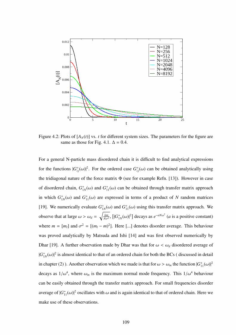
0 5 10 15 20 25t
0
0.002
0.004
0.006
0.008
0.01
0.012
[AN
(t)]
N=128N=256N=512N=1024N=2048N=4096N=8192
Figure 4.2: Plots of [AN(t)] vs. t for different system sizes. The parameters for the figure aresame as those for Fig. 4.1. ∆ = 0.4.
For a general N-particle mass disordered chain it is difficult to find analytical expressions
for the functions |G+i j(ω)|2. For the ordered case G+i j(ω) can be obtained analytically using
the tridiagonal nature of the force matrix Φ (see for example Refn. [13]). However in case
of disordered chain, G+1N(ω) and G+11(ω) can be obtained through transfer matrix approach
in which G+1N(ω) and G+11(ω) are expressed in terms of a product of N random matrices
[19]. We numerically evaluate G+1N(ω) and G+11(ω) using this transfer matrix approach. We
observe that at large ω > ωd =
√km
Nσ2 ,[|G+1N(ω)|2
]decays as e−aNω2
(a is a positive constant)
where m = [ml] and σ2 = [(ml − m)2]. Here [...] denotes disorder average. This behaviour
was proved analytically by Matsuda and Ishi [14] and was first observed numerically by
Dhar [19]. A further observation made by Dhar was that for ω < ωd disordered average of
|G+1N(ω)|2 is almost identical to that of an ordered chain for both the BCs ( discussed in detail
in chapter (2) ). Another observation which we made is that forω > ωm the function |G+11(ω)|2
decays as 1/ω4, where ωm is the maximum normal mode frequency. This 1/ω4 behaviour
can be easily obtained through the transfer matrix approach. For small frequencies disorder
average of |G+11(ω)|2 oscillates with ω and is again identical to that of ordered chain. Here we
make use of these observations.
109

After integrating Eq. (4.58) numerically, we obtain Ai(t) and Gi j(t) and hence g0(t) for dif-
ferent system sizes with different disorder configurations. In Fig. 4.1 we plot [g∆T (t)] versus
t for system sizes N = 4, 8 and 16 with free BC. We observe that the correlation functions
for two system sizes remain almost identical at short times and start being different signif-
icantly after some time scale. These observations can be made by looking at the dominant
contributions of ω2|G+1i(ω)|2 in the integrand of Eq. (4.58) for fixed t. At large ω the func-
tion |G+1N(ω)|2 decays as e−aNω2(a is a positive constant)[14, 19] whereas |G+11(ω)|2 decays as
1/ω4. At small frequencies both G+1N(ω) and G+11(ω) are oscillating functions of ω and the
frequency of oscillation increases with system size N. As a result A1(t) is independent of
system size N at small times and starts depending on N after some time scale, where con-
tribution from small ω becomes important. Whereas, in case of AN(t), only a small range
of ω contributes to the Fourier transform of ω2|G+1N(ω)|2(Eq. (4.58)). For large N, at small
times A1(t) is much larger that AN(t) and contributes most in g0(t), which makes g0(t) to be
independent of N at small times. Inset in Fig. 4.1 compares A1(t) and AN(t) for N = 8. In the
next paragraph we will see that physically interesting quantities like current, fluctuations in
current in NESS are related to the time integral of C∆T (t) and this integral depends only on
AN(t), though A1(t) has dominant contribution in the correlation function itself. Hence it is
more relevant to see the behaviour of AN(t) with system size N. In Fig. 4.2 we plot [AN(t)]
for different system sizes. Here we prefer to give plots of disorder-averaged quantities.
Let Q(τ) =∫ τ
odt j1,L(t) be the heat transfer in duration τ from left reservoir to the system.
Using stationarity property of the correlation function it is easy to show that the 2nd order
cumulant of Q(τ) is related to C∆T (t) as
limτ→∞
〈Q2(τ)〉cτ
=
∫ ∞
0dtC∆T (t). (4.71)
Now integrating the expression of C∆T (t) given in Eq. (4.69) from 0 to∞ and again using the
identity in Eq.(4.55) we get∫ ∞
0dtC∆T (t) = 2γLγRTLTRK2
BAN(0) + 8γ2Lγ
2RK2
B(TL − TR)2∫ ∞
0dt A2
N(t) . (4.72)
110

In the frequency space the Eq. (4.72) can be written as an integration over ω of the transmis-
sion coefficient T (ω) defined in Eq. (4.61) and we obtain∫ ∞
0dtC∆T (t) =
K2BTLTR
2π
∫ ∞
0dω T (ω) +
K2B(TL − TR)2
4π
∫ ∞
0dω T 2(ω) . (4.73)
This expression matches with the expression given in [100] for quantum mechanical systems
in the high temperature limit. Now if we put TL = TR = T in the expression in Eq. (4.72)
and use Eq.(4.56) we get a relation between the current in the non-equilibrium steady state
and the equilibrium correlation function similar to the GK relation given in Eq. (4.20) of the
previous section ∫ ∞
0dtC0(t) =
K2BT 2
2π
∫ ∞
0dω T (ω) = KBT 2 J
(TL − TR), (4.74)
where C0(t) is the equilibrium auto-correlation function for the open system. The inset of
Fig. 4.3 shows the system size dependence of the disorder average of current.
In general for large system sizes [J] and [ 〈Q2(τ)〉cτ
] scale with N as N−β and N−α respectively.
Using the frequency dependence of T (ω) = [T (ω)] and [T 2(ω)] one can predict the values
of α and β for different BC’s. By computing [J] in NESS, several authors have already
studied asymptotic size dependence of [J]. Rubin and Greer [101] obtained β = 1/2 for
free BC, which was latter proved rigorously by Verheggen[102]. Casher and Lebowitz [17]
studied the same model and obtained a lower bound for [J] ≥ N−3/2 and simulations by
Rich and Vischer [103] confirmed the exponent to be β = 3/2. Later Dhar[19] obtained J
for both the boundary conditions using Langevin Equation and Green Function approach and
obtained β = 1/2 for free BC and β = 3/2 for fixed BC. Here we follow the same procedure
described in [19] to find the asymptotic size dependence of [ 〈Q2(τ)〉cτ
] from the expression
given in Eq. (4.73).
We numerically observe that for both the BCs [T 2(ω)] is much smaller than T (ω) for
each N. Hence, in determining the asymptotic N dependence, dominant contribution comes
from the integration of T (ω) over ω. To determine α, we use the fact (discussed in the first
paragraph of this section) that for ω greater than ωd ∼ N−1/2, T (ω) decays exponentially
111
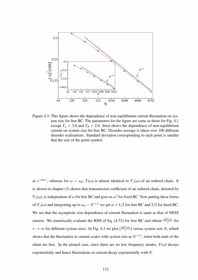
64 128 256 512 1024 2048 4096 8192N
0.125
0.25
0.5
[<Q
2 (τ)>
/τ]
64 128 256 512 1024 2048 4096 8192N
0.0625
0.125
0.25
0.5[<
j L>
] N-1/2
N-1/2
Figure 4.3: This figure shows the dependence of non-equilibrium current fluctuation on sys-tem size for free BC. The parameters for the figure are same as those for Fig. 4.1except TL = 3.0 and TR = 2.0. Inset shows the dependence of non-equilibriumcurrent on system size for free BC. Disorder average is taken over 100 differentdisorder realizations. Standard deviation corresponding to each point is smallerthat the size of the point symbol.
as e−aNω2, whereas for ω < ωd, T (ω) is almost identical to To(ω) of an ordered chain. It
is shown in chapter (3) shown that transmission coefficient of an ordered chain, denoted by
To(ω), is independent of ω for free BC and goes as ω2 for fixed BC. Now putting these forms
of To(ω) and integrating up to ωd ∼ N−1/2 we get α = 1/2 for free BC and 3/2 for fixed BC.
We see that the asymptotic size dependence of current fluctuation is same as that of NESS
current. We numerically evaluate the RHS of Eq. (4.72) for free BC and obtain 〈Q2(τ)〉cτ
for
τ → ∞ for different system sizes. In Fig. 4.3 we plot [ 〈Q2(τ)〉cτ
] versus system size N, which
shows that the fluctuation in current scales with system size as N−1/2, when both ends of the
chain are free. In the pinned case, since there are no low frequency modes, T (ω) decays
exponentially and hence fluctuations in current decay exponentially with N.
112

4.6 Conclusions
In this chapter we have derived an exact expression for the linear response conductance in
a system connected to heat baths. Our results are valid in arbitrary dimensions and have
been derived both for a solid where particles execute small displacements about fixed lat-
tice positions as well as for a fluid system where the motion of particles is unrestricted, and
various heat bath models have been considered. We also have given an expression for the
boundary current-current correlation for a one dimensional mass-disordered harmonic sys-
tem in NESS. The correlation function has been expressed in terms of the phonon Green’s
functions which are easy to evaluate numerically. We show that the integration of equilib-
rium correlation function gives current satisfying the finite size open system Green-Kubo
formula whereas the integration of non-equilibrium correlation function gives information
about current fluctuation in the NESS.
The important differences with the usual Green-Kubo formula are worth noting. In the
present formula, one does not need to first take the limit of infinite system size; the result is
valid for finite systems. The fact that a sensible answer is obtained even for a finite system
(unlike the case for the usual Green-Kubo formula) is because here we are dealing with an
open system. Secondly the correlation function here has to be evaluated not with Hamilto-
nian dynamics, but for an open system evolving with heat bath dynamics. Finally we note
that unlike the usual derivation of the Green-Kubo formula where the assumption of local
thermal equilibrium is crucial, the present derivation requires no such assumption. The re-
sults are thus valid even for integrable Hamiltonian models, the only requirement being that
they should attain thermal equilibrium when coupled to one or more heat reservoirs all at the
same temperature.
Our derivation here is based on using both the microscopic equations of motion and also
the equation for the phase space distribution. The broad class of systems and heat baths for
which we have obtained our results strongly suggests that they are valid whenever detailed
balance is satisfied.
113

4.7 appendix
4.7.1 Proof of Eq. [4.55]
Let us first define few quantities:
G = M12 GM
12 , Γ = M−
12ΓM−
12 and Φ = M−
12ΦM−
12
Using this above definitions Eq. (4.50) can be written as
¨G(t) + Γ ˙G(t) + ΦG(t) = 0. (4.75)
We use the above equation to evaluate ddt′ [
˙GT (t′) ˙G(t′ + t)] and get
ddt′
[ ˙GT (t′) ˙G(t′ + t)] = −2 ˙GT (t′)Γ ˙G(t′ + t) +d
dt′[GT (t′)ΦG(t′ + t)].
Now integrating both side of the above equation over t′ = 0 to t′ = ∞ we get
˙G(t) = 2∫ ∞
0dt′ ˙GT (t′)Γ ˙G(t′ + t). (4.76)
To the above equation we have used the following: G(0) = M−1, G(0) = 0, G(t) → 0 as
t → ∞. Now we know that Γi j = ( γLm1δi1 +
γRmNδiN)δi j. Taking (11)th element on the both side
of the matrix equation (4.76) we get
G11(t)2
=
∫ ∞
0dt′[γLG11(t′)G11(t′ + t) + γRG1N(t′)G1N(t′ + t)]
= γLA1(t) + γRAN(t). (4.77)
4.7.2 Expressions of K1s
K(1)1 (t1, t2, t3, t4, t) =
[γ2
LT 2LG11(t − t1)G11(t − t2)G11(−t3)G11(−t4)
+γ2RT 2
RG1N(t − t1)G1N(t − t2)G1N(−t3)G1N(−t4)
+γLTLγRTRG1N(t − t1)G1N(t − t2)G11(−t3)G11(−t4)
+G11(t − t1)G11(t − t2)G1N(−t3)G1N(−t4)],
114

K(2)1 (t1, t2, t3, t4, t) =
[γ2
LT 2LG11(t − t1)G11(t − t2)G11(−t3)G11(−t4)
+γ2RT 2
RG1N(t − t1)G1N(t − t2)G1N(−t3)G1N(−t4)
+γLTLγRTRG1N(t − t1)G11(t − t2)G1N(−t3)G11(−t4)
+G11(t − t1)G1N(t − t2)G11(−t3)G1N(−t4)]
and
K(3)1 (t1, t2, t3, t4, t) =
[γ2
LT 2LG11(t − t1)G11(t − t2)G11(−t3)G11(−t4)
+γ2RT 2
RG1N(t − t1)G1N(t − t2)G1N(−t3)G1N(−t4)
+γLTLγRTRG11(t − t1)G1N(t − t2)G1N(−t3)G11(−t4)
+G1N(t − t1)G11(t − t2)G11(−t3)G1N(−t4)].
115
5 Large deviations in transportprocesses
In this chapter our interest is in predicting probabilities of rare fluctuations in transport pro-
cesses. A number of interesting results have been obtained recently on large fluctuations
away from typical ones in nonequilibrium systems. These results include various fluctua-
tion theorems[104, 105, 106, 107, 108, 109, 100] and the Jarzynski relation [110]. In the
context of transport one typically considers an observable, say Q, such as the total number
of particles or heat transferred across an object with an applied chemical potential or tem-
perature difference respectively. For a given observation time τ this is a stochastic variable
and one is naturally interested in its probability distribution R(Q, τ). Various general results
that have been obtained for R(Q, τ) give some quantitative measure of the probability of rare
fluctuations. Usually, for large τ the probabilities of large fluctuations show scaling behavior
P(Q, τ) ∼ e−τ F(Q/τ). The function F(q) is called the large deviation function which provides
informations about the tails of the distribution i.e. the probabilities of large fluctuations. For
a few model systems exact results have been obtained for the large deviation function F(q)
[108, 109, 100]. Very often the characteristic function of P(Q, τ), given by⟨e−λQ⟩
also has
a similar scaling⟨e−λQ⟩
∼ eτ µ(λ), where µ(λ) is defined as µ(λ) = limτ→∞ τ−1 ln
⟨e−λQ⟩
. The
large deviation function F(q) is related to µ(λ) by a Legendre transformation. Often it is eas-
ier to calculate µ(λ) rather than F(q) directly. One can then obtain F(q) from µ(λ) by doing
Legendre transform. In the first section of this chapter we calculate µ(λ) corresponding to
the distribution of heat flow across a harmonic chain. We express µ(λ) as an integration of
some function of the phonon transmission coefficient T (ω).
Computing the tails of P(Q, τ) for any system is also difficult both in experiments and in
116
computer simulations, since the generation of rare events requires a large number of trials.
Recently an efficient algorithm has been proposed [111] to compute the function µ(λ). In
the second section of this chapter we present an algorithm for generating rare events very
often and computing their probabilities. The algorithm proposed here is complementary
to the one discussed in [111] in the sense that we obtain P(Q, τ) directly whereas [111]
obtains µ(λ) directly. However, as has been pointed out in [112] there may be problems in
obtaining the tails of µ(λ) using the algorithm of [111]. Our algorithm, based on the idea of
importance sampling, computes P(Q, τ) for any given τ and accurately reproduces the tails
of the distribution. Algorithms based on importance sampling have earlier been proposed for
the study of transition rate processes [113, 114, 115].
This chapter is organised as follows. In Sec.(5.1) we present the calculation of µ(λ) for
the heat flow across a harmonic system. In the subsection (5.1.1) we calculate µ(λ) for a har-
monic chain of length N. Then in subsection (5.1.2) we discuss the case of single Brownian
particle as an example with small discussion on the case of two particles connected by har-
monic spring. In the last section (5.2) we present the algorithm of finding the probabilities
of rare events. First we develop the algorithm on general basis and we apply this algorithm
to different transport processes in the next few subsections.
5.1 Large deviation function of heat flow in harmonicchain
We consider a mass disordered harmonic chain of N particles described by the Hamiltonian
H :
H =N∑
l=1
12
mlv2l +
12
N∑l=1
N∑m=1
Φlmxlxm (5.1)
where xl is displacement of lth particle about its equilibrium position, vl is its velocity, ml is
its mass and Φ represents the force constant matrix. The particles 1 and N are connected to
two white noise heat baths of temperatures TL and TR respectively. The equation of motion
117

of the lth particle is given by [19]
xl = vl ; mlvl = −
N∑m=1
Φlmxm + δl,1[−γLv1 + ηL] + δl,N[−γRvN + ηR ]
where l = 1, 2...N and x0 = xN+1 = 0 (5.2)
and ηL,R(t) are Gaussian noise terms with zero mean and related to the dissipative terms
through the relations
〈ηL,R(t)ηL,R(t′)〉 = 2γL,RTL,Rδ(t − t′)
〈ηL(t)ηR(t′)〉 = 0, 〈ηL,R(t)〉 = 0. (5.3)
Since the potentials are quadratic in positions, it is convenient to write the set of equations
in Eq. (5.2) in the form of linear matrix equation as follows:
X = V, MV = −ΓV − ΦX + η(t), (5.4)
where X = (x1, x2, ..., xN)T , V = (v1, v2, ..., vN)T and M = diag(m1,m2, . . . ,mN) is the diago-
nal mass matrix. The diagonal matrix Γ describes the dissipation, Γi, j = δi, j(δi,1γL + δi,NγR),
and ηi(t) = δi,1ηL(t) + δi,NηR(t). In some time duration τ there will be a net amount of heat
transfer Q(τ) between the left reservoir and the system in the steady state. This is given by
Q(τ) =∫ τ
0
[ηL(t) − γLv1(t)
]v1(t) dt. (5.5)
Clearly, Q(τ) is a random variable whose value depends on the realization of noise η(t) :
0 ≤ t ≤ τ and on the initial condition. Here we are interested in the probability distribution
of Q(τ) given that the initial conditions are chosen from the non-equilibrium steady state
(NESS) of the system. We denote this distribution by R(Q, τ). We are mainly interested in
probabilities of large fluctuations in Q for large τ (τ → ∞). Often it is difficult to obtain an
analytical expression for the probability density function (pdf) R(Q, τ), but it is easier to find
the characteristic function of Q(τ), defined as 〈e−λQ〉 =∫
dQ exp(−λQ) R(Q, τ) = R(λ, τ).
Let the pdf of Q(t) for given initial and final configurations of the system be denoted by
P(Q,U, t|U0) where, U = [VT , XT ]T represents the state of the system i.e. velocities and
118

positions of all the particles at some time t. In some cases, for example harmonic chain with
open boundaries, a steady state distribution does not exist with U = [VT , XT ]T . In such cases
one has to chose U properly, like for open boundary case U = [VT , x2 − x1, ....., xN − xN−1]T .
The distribution P(Q,U, t|U0) satisfies the following Fokker-Planck equation :
∂P∂t=
[ 2N∑l=1
∂
∂Ul
〈∆Ul〉
∆t+
∂
∂Q〈∆Q〉∆t+
2N∑l=1
2N∑m=1
∂2
∂Ul∂Um
〈∆Ul∆Um〉
∆t
+
2N∑l=1
∂2
∂UlQ〈∆Ul∆Q〉∆t
+∂2
∂Q2
〈∆Q2〉
∆t
]P(Q,U, t|U0) ; with ∆t → 0 , (5.6)
where the moments are calculated using the Langevin equations (5.4) and heat equation given
in Eq. (5.5). After calculating the moments we get
∂P∂t= LQ P(Q,U, t|U0)
where LQ =
N∑l=1
[∂H∂xl
∂
∂vl−∂H∂vl
∂
∂xl
]+ γL
∂
∂v1v1 + γR
∂
∂vNvN + (γLv2
1 − γLTL)∂
∂Q
+ γLTL∂2
∂v21
+ γRTR∂2
∂v2N
+ γLTLv21∂2
∂Q2 + 2γLTL∂2
∂v1∂Qv1. (5.7)
Let the characteristic function of Q corresponding to P(Q,U, t|U0) is defined as
P(λ,U, t|U0) =⟨e−λQδ(U(t) − U)
⟩U0=
∫dQ exp(−λQ) P(Q,U, t|U0). (5.8)
The evolution equation corresponding to P(λ,U, t|U0) is obtained by Fourier transforming
both sides of Eq. (5.7) and is given by
∂P∂t= Lλ P(λ,U, t|U0)
where Lλ =N∑
l=1
[∂H∂xl
∂
∂vl−∂H∂vl
∂
∂xl
]+ γL
∂
∂v1v1 + γR
∂
∂vNvN + (γLv2
1 − γLTL) λ
+ γLTL∂2
∂v21
+ γRTR∂2
∂v2N
+ γLTLv21λ
2 + +2γLTLλ∂
∂v1v1. (5.9)
The solution of the above equation can formally be written down in the eigenbases of the
119
Fokker-Planck operator Lλ, and the large t behavior is dominated by the term having the
largest eigenvalue µ(λ), i.e.,
P(λ,U, t|U0) ≈ χ(U0, λ)Ψ(U, λ) exp[t µ(λ)] (5.10)
whereΨ(U, λ) is the eigenfunction corresponding to the largest eigenvalue, i.e.,LλΨ(U, λ) =
µ(λ)Ψ(U, λ), and χ(U0, λ) is the projection of the initial state onto eigenstate corresponding
to the eigenvalue µ(λ). The existence of a unique steady state of the system demands that
for λ = 0 the largest eigenvalue µ(0) = 0. Moreover, χ(U0, 0) = 1 and Ψ(U, 0) is the steady
state pdf, which is a Gaussian in our case with the covariance matrix limt→∞〈UUT 〉. Using
Eq. (5.10), for large τ,
R(λ, τ) ≈ g(λ) exp[τµ(λ)
], (5.11)
where g(λ) =∫χ(U0, λ)Ψ(U0, 0) dU0
∫Ψ(U, λ) dU, and we note that g(0) = 1.
The large τ behavior of the pdf R(Q, τ) can be obtained by the saddle-point approximation
of the integral
R(Q, τ) = (2πi)−1∫ i∞
−i∞R(λ, τ)eλQ dλ,
while using the approximation given by Eq. (5.11) for the integrand. This leads to the large
deviation form of the pdf, R(Q, τ) ∼ exp[−τ F(Q/τ)], meaning
limτ→∞
τ−1 ln P(qτ, τ) = −F(q).
The large deviation function is given by, F(q) = −[µ(λ∗) + λ∗q], with λ∗(q) implicitly given
by the saddle point equation µ′(λ∗) = −q, provided that g(λ) is analytic along the real λ in
the region [0, λ∗], so that, (i) g(λ) can be neglected from the above saddle-point calculation
as sub-leading contribution, and (ii) the contour of the integration can be deformed smoothly
through saddle point λ∗. In this case, if µ(λ) possesses the symmetry µ(λ) = µ(a − λ) then
the so-called fluctuation relation F(q) − F(−q) = −aq is verified. On the other hand, if
g(λ) possesses any singularity in [0, λ∗], then one needs to include g(λ) in the saddle point
calculation, and in that case even though µ(λ) possesses above mentioned symmetry, F(q)
120

may not satisfy the fluctuation relation. This has been discussed in great details in [117,
118, 109]. We shall not elaborate on this issue here. Rather, the aim is to obtain an exact
expression for µ(λ), which according to Eq. (5.11),
µ(λ) = limτ→∞
1τ
ln⟨e−λQ⟩
. (5.12)
Our main result is the exact expression
µ(λ) = −1
4π
∫ ∞
−∞
dω ln[1 + T (ω)TLTRλ(∆β − λ)
], (5.13)
where ∆β = T−1R − T−1
L , and
T (ω) = 4γLγRω2G1,N(ω)G1,N(−ω), (5.14)
with G(ω) = [Φ − ω2 M + iωΓ]−1. (5.15)
The function T (ω) was introduced earlier in Eq.(2.38) and is the phonon transmission coef-
ficient. From Eq. (5.13), we note that µ(0) = 0 as required. It is also evident that Eq. (5.13)
possesses the symmetry µ(λ) = µ(∆β − λ). In general, if the operator Lλ and its adjoint L†λ
possess the symmetryL†λ = La−λ, then it is easily shown that µ(λ) = µ(a−λ), without requir-
ing its explicit form. Even if after doing a similarity transformation the operator Lλ possess
the symmetry L†λ = La−λ, then also µ(λ) has the above symmetry. However, this is not the
case for the system discussed here. In fact, even for the simplest case of just one particle
connected to two heat reservoirs [109], the Fokker-Planck operator does not possesses the
above mentioned symmetry. Although, in this case the Fokker-Planck operator (of one vari-
able) can be transformed to a Hermitian operator of quantum harmonic oscillator, where the
potential remains invariant under λ → (∆β − λ). We are not aware of such a transformation
for the system having more than one particles discussed in this chapter.
Using Eq. (5.13), one can immediately find the expression for the average energy current,
limτ→∞
〈Q〉τ= −µ′(0) =
TL − TR
4π
∫ ∞
−∞
dωT (ω).
which is in agreement with previous results [19, 17, 15, 69]. It is clear from the above expres-
121

sion that the average current is sum of the different contributions for different phonon modes
which is determined by the individual phonon transmission coefficient T (ω). In the next few
sections we present the derivation of our results. We start by calculating P(λ,U, τ|,U0) .
5.1.1 Derivation
We first obtain an expression for P(λ,U, τ|,U0), from which we get χ(U0, λ) Ψ(U, λ) and
µ(λ) after proper identification with Eq. (5.10). From Eq. (5.8) we see that P(λ,U, τ|,U0)
is actually noise average of e−λQδ(X − X(τ))δ(V − V(τ)), where noises are chosen from a
Gaussian distribution. As usual replacing the δ functions by their integral representations
δ(X − X(τ)) =∫
....
∫dσ
(2π)N eiσ.(X−X(τ)), where σ = (σ1, σ2, ...σN)T
δ(V − V(τ)) =∫
...
∫dρ
(2π)N eiρ.(V−V(τ)), where ρ = (ρ1, ρ2, ...ρN)T . (5.16)
we write
P(λ,U, τ|,U0) =∫
...
∫ N∏l=1
dσl
2πeiσl xl
N∏l=1
dρl
2πeiρlvl
⟨eA(τ)⟩
where, A(τ) = −λQ − iN∑
l=1
[σlxl(τ) + ρlvl(τ)]. (5.17)
There are three steps to calculate⟨eA⟩.
• (i) At first, we express X(τ) and V(τ) in terms of noise configurations by solving the
equations in (5.4) for given X(0) and V(0).
• (ii) Second, using these expressions of X(τ) and V(τ) we show that Q(τ) is quadratic
in η(t) and hence A(τ) has quadratic, linear and noise independent terms.
• (iii) Finally, we take average of eA over noise configurations. Since η(t) is Gaussian
noise and A(τ) depends on the noise atmost quadratically,⟨eA(τ)⟩ can be expressed as
a Gaussian integral over noise variables.
It is more convenient to do the above procedure in the Fourier space, because while taking
the noise average in the time domain one has to do a Gaussian path integration over noise
122
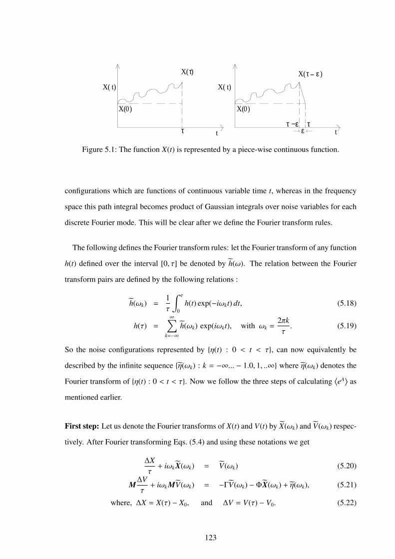
X( )t
X( )0
X(τ)
tτ
0X( )
− ε
τ −εtε
τX( )
X( )t
τ
Figure 5.1: The function X(t) is represented by a piece-wise continuous function.
configurations which are functions of continuous variable time t, whereas in the frequency
space this path integral becomes product of Gaussian integrals over noise variables for each
discrete Fourier mode. This will be clear after we define the Fourier transform rules.
The following defines the Fourier transform rules: let the Fourier transform of any function
h(t) defined over the interval [0, τ] be denoted by h(ω). The relation between the Fourier
transform pairs are defined by the following relations :
h(ωk) =1τ
∫ τ
0h(t) exp(−iωkt) dt, (5.18)
h(τ) =∞∑
k=−∞
h(ωk) exp(iωkt), with ωk =2πkτ. (5.19)
So the noise configurations represented by η(t) : 0 < t < τ, can now equivalently be
described by the infinite sequence η(ωk) : k = −∞... − 1.0, 1, ..∞ where η(ωk) denotes the
Fourier transform of η(t) : 0 < t < τ. Now we follow the three steps of calculating⟨eA⟩ as
mentioned earlier.
First step: Let us denote the Fourier transforms of X(t) and V(t) by X(ωk) and V(ωk) respec-
tively. After Fourier transforming Eqs. (5.4) and using these notations we get
∆Xτ+ iωk X(ωk) = V(ωk) (5.20)
M∆Vτ+ iωk MV(ωk) = −ΓV(ωk) − ΦX(ωk) + η(ωk), (5.21)
where, ∆X = X(τ) − X0, and ∆V = V(τ) − V0. (5.22)
123

Solving the above equations for X(ωk) and V(ωk) in terms of ∆X, ∆V and η we get :
X = G[η −
1τ
M∆V +1
iτωk(Φ −G−1)∆X
], (5.23)
V = G[iωkη −
iωk
τM∆V +
1τΦ∆X
], (5.24)
where,
X(τ) = limε→0
∞∑k=−∞
X(ωk) exp(−iωkε)
V(τ) = limε→0
∞∑k=−∞
V(ωk) exp(−iωkε). (5.25)
and G is given in Eq. (5.15). While representing the continuous function X(t) : 0 ≤ t ≤ τ
in terms of Fourier series we have approximated the function X(t) by a piecewise continuous
function with ε → 0 as shown in the Fig. (5.1). Same holds for V(τ) also.
Using the above expressions for X(ωk) and V(ωk), one can easily show that for large τ
X(τ) = limε→0
∞∑k=−∞
Gη exp(−iωkε) (5.26)
X(τ) = limε→0
∞∑k=−∞
iωGη exp(−iωkε), (5.27)
where we have used the fact that other terms of the form
1τ
∞∑k=−∞
G(ωk) f (∆X,∆V,M, ωk) exp(−iωkε) (5.28)
go to zero in the limit τ→ ∞. It can easily be seen by converting the above summation into a
contour integral on a semicircle in the lower half plane and noting that all the poles of G(ωk)
lie in the upper half plane.
Thus we have expressed all relevant variables in terms of new noise variables ηL,R(ωk),
which have the following correlations:
⟨ηα(ωk )ηα′(ω′k)
⟩= 2δα,α′
γαTα
τδωk ,−ω
′k
with, α, α′ = L,R. (5.29)
Now we follow the remaining two [(ii) and (iii)] steps of calculating⟨eA(τ)⟩. For convenience
of calculation, from now onwards we suppress the subscript k in ωk.
124
Second step : With the help of Eq. (5.19) we convert the two time integrals over [0, τ] in
Eq. (5.5) into two infinite series summations over ω and finally get
Q(τ) = τ
∞∑k=−∞
[ηL(ω)v1(−ω) − γLv1(ω)v1(−ω)
]. (5.30)
Putting this expression of Q(τ) and expressions of X(τ) and V(τ) from Eqs. (5.26) and (5.27)
into Eq. (5.17) we get
A(τ) = −λτ∞∑
k=−∞
[ηL(ω)v1(−ω) − γLv1(ω)v1(−ω)
+i
[g1(ω)ηL(ω) + g2(ω)ηR(ω)
]e−iωε
]. (5.31)
where, v1(ω) = iω(G11ηL(ω) +G1N ηR(ω))e−iωε +1τ
N∑m=1
G1m fm(ω) (5.32)
with fm(ω) =∑
j
Φm j∆X j − iωMm∆Vm.
In the above we have introduced three new functions g1(ω), g2(ω) and g(ω) which are given
by
g1(ω) =N∑
m=1
Gm1(σm + iωρm),
g2(ω) =N∑
m=1
GmN(σm + iωρm)
and g(ω) =N∑
m=1
G1m fm respectively.
Now we show that A(τ) can be expressed as a sum of quadratic, linear and noise inde-
pendent terms. Before doing that we introduce some more notations. We denote real and
imaginary parts of ηL,R(ω) as follows:
ηL(ω) = ξL1(ω) − iξL2(ω) and ηR(ω) = ξR1(ω) − iξR2(ω) (5.33)
where each ξ′s are independent Gaussian noise with zero mean and have the following cor-
relations
〈ξLi(ω)ξL j(ω′)〉 = δi jDL
τ[δω,ω′ + δω,−ω′]
125

〈ξRi(ω)ξR j(ω′)〉 = δi jDR
τ[δω,ω′ + δω,−ω′]
〈ξLi(ω)ξR j(ω′)〉 = 0,
where, DL = γLTL and DR = γRTR. (5.34)
From Eq. (5.32) we note that v1(ω) is linear in ξ′s. Hence it is clear from Eq. (5.31) that A(τ)
has terms quadratic and linear in noise and as well as terms independent of noise. To write
A(τ) as a sum of quadratic, linear and noise independent terms separately we first write A(τ)
in the following form:
A(τ) = s(0) +∞∑
k=1
[s(ω) + s(−ω)]
where, s(ω) = −λτ[ηL(ω)v1(−ω) − γLv1(ω)v1(−ω)
]−i
[g1(ω)ηL(ω) + g2(ω)ηR(ω)
]e−iωε . (5.35)
Note that s(−ω) is the complex conjugate of s(ω). Putting V1(ω) from Eq. (5.32) in the
expression of s(ω) in Eq. (5.35) and using the expressions for ηL,R(ω) given in Eq. (5.33), we
write A(τ) in the following form
A(τ) = s(0) +∞∑
k=1
[−λτ
2ξT (ω)E(ω)ξ(ω) + JT (λ, ω)ξ(ω) + c(ω)
]. (5.36)
where ξ(ω) = [ξL1(ω), ξL2(ω), ξR1(ω), ξR2(ω)]T , E(ω) is a 4 × 4 matrix, J(λ, ω) is a 4 × 1
column vector and c(ω) is a complex number. From the above equation one can easily note
that E(ω) does not depend on the initial and final configuration whereas Jλ(ω) and c(ω) do
depend. In the appendix we give explicit forms of E(ω), J(λ, ω) and c(ω).
Third step : In this step we take average over noises to calculate 〈eA(τ)〉. Noise average of
eA(τ) can be written as
〈eA(τ)〉 =∏
k
&dξL1(ω)dξL2(ω)dξR1(ω)dξR2(ω) P(ξL1, ξL2, ξR1, ξR2) exp
[A(τ)
],
where P(ξL1, ξL2, ξR1, ξR2) =τ2
4π2DLDRexp
[−τ
2ξT diag
( 1DL
,1
DL,
1DR
,1
DR
)ξ], (5.37)
126
is the joint probability distribution of the noise variables [ξL1(ω), ξL2(ω), ξR1(ω), ξR2(ω)].
Now putting the expression of A(τ) from Eq. (5.36) in the argument of the exponential we
get
〈eA(τ)〉 = [τ
2π√
D1D2
"dξL1(0)dξR1(0) P(ξL1, ξR1) e−s(0)]
×
∞∏k=1
τ2
4π2D1D2
&dξL1(ω)dξL2(ω)dξR1(ω)dξR2(ω)
exp∞∑
k=1
[−τ
2ξT (ω)Σλ(ω)ξ(ω) + JT
λ (ω)ξ(ω) + c(ω)]
where Σλ(ω) = λE(ω) + diag(1
DL,
1DL
,1
DR,
1DR
). (5.38)
After doing the Gaussian integration over the noises and after some rearrangements we fi-
nally get
⟨eA(τ)⟩ = 4
√detΣ0(0)detΣλ(0)
exp[ 14τ
JT (λ, 0)Σ−1λ (0)J(λ, 0) +
12
c(0)]
×
∞∏k=1
√detΣ0(ω)detΣλ(ω)
exp ∞∑
k=1
[12τ
JT (λ, ω)Σ−1λ (ω)J(λ, ω) + c(ω)]
. (5.39)
Including the k = 0 term one can write 〈eA(τ)〉 in the following compact form
⟨eA(τ)⟩ = 4
√detΣ0(0)detΣλ(0)
∞∏k=1
√detΣ0(ω)detΣλ(ω)
exp ∞∑
k=−∞
[14τ
JT (λ, ω)Σ−1λ (ω)J(λ, ω) +
12
c(ω)].(5.40)
This completes the three steps of calculating 〈eA(τ)〉.
Now putting this expression for 〈eA(τ)〉 in Eq. (5.17) we get the following expression
P(λ,U, τ|,U0) =(
4
√detΣ0(0)detΣλ(0)
∞∏k=1
√detΣ0(ω)detΣλ(ω)
)×
( ∫...
∫ N∏l=1
dσl
2πeiσl xl
N∏l=1
dρl
2πeiρlvl
exp ∞∑
k=−∞
[14τ
JT (λ, ω)Σ−1λ (ω)J(λ, ω) +
12
c(ω)]). (5.41)
127

We Compare the r.h.s. of the above equation with r.h.s. of Eq. (5.10), while noting that Σλ
does not depend on µ, ν, ∆X, ∆V whereas the expression in the exponent does, and identify
µ(λ) =12τ
∞∑k=0
ln[detΣ0(ω)detΣλ(ω)
]+
14τ
ln[detΣ0(0)detΣλ(0)
](5.42)
and χ(U0, λ)Ψ(U, λ) =∫
...
∫ N∏l=1
dσl
2πeiσl xl
N∏l=1
dρl
2πeiρlvl
exp ∞∑
k=−∞
[14τ
JTλ Σ−1λ Jλ +
12
(c(ω) + c(−ω))]. (5.43)
From the explicit form of Σλ(ω) one can calculate detΣλ(ω) and get
detΣλ(ω)detΣ0(ω)
=[1 + T (ω)TLTRλ(∆β − λ)
]2 . (5.44)
Above we have made use of the identity:
iω2
[G1,1(ω) −G1,1(−ω)
]= ω2[γLG1,1(ω)G1,1(−ω) + γRG1,N(ω)G1,N(−ω)
](5.45)
which can be proved as follows. From Eq.(5.15) we have G−1(ω) −G−1(−ω) = 2iωΓ. Mul-
tiplying by G(ω) from left and by G(−ω) from right on the both sides of the equation in the
previous line we get G(−ω) −G(ω) = 2iωG(ω)ΓG(−ω). After multiplying both sides by iω
and comparing the 11th element from both sides we get the above identity. Same identity has
been obtained in Eq. (4.55) but in time domain and from this one can get the present one by
Fourier transforming both sides.
In τ→ ∞ limit, converting the summation over k in Eq. (5.42) into integration over ω we
get the following exact expression for µ(λ) :
µ(λ) = −1
4π
∫ ∞
−∞
dω ln[1 + T (ω)TLTRλ(∆β − λ)
]. (5.46)
For the case when all the masses are equal to m, after some algebra one gets det G−1(ω) =
[a(q) sin Nq + b(q) cos Nq]/ sin q, where 2 cos q = 2 − mω2, and
a(q) = (2 − ω2γLγR) cos q − 2 + iω(γL + γR)(1 − cos q),
b(q) = [ω2γLγR + iω(γL + γR)] sin q.
128

Therefore, one has
T (ω) =4γLγRω
2 sin2 q∣∣∣a(q) sin Nq + b(q) cos Nq∣∣∣2 . (5.47)
Using Eq. (5.47), it is straight forward to numerically compute the integral in Eq. (5.46) for
any finite N. The integration in Eq. (5.43) is actually a Gaussian integration over σi and ρ′is,
since the exponent of the exponential can be expressed as a quadratic polynomial in σ and ρ
variables. It is very difficult to do the integrations in Eqs. (5.46) and (5.43) analytically for a
general N particle harmonic chain. There are few cases where these two integrations can be
done analytically. Below we consider one such case.
5.1.2 Single Brownian particle
The Langevin equation for a single Brownian particle is given by :
v = −(γL + γR)v + ηL(t) + ηR(t), (5.48)
where v is the velocity of the particle. Here we consider the velocity of the particle and not
the position, since velocity v of the particle will have a normalized steady state distribution
whereas position will not have one, and the heat transfer Q, in which we are interested,
does not depend on position. For single Brownian particle the matrix defined in Eq. (5.15)
becomes a complex number: G−1(ω) = −ω2 + iωγ where γ = γL + γR. For this case explicit
forms for the matricesALL, ALL andALL (defined in appendix 5.4.1 ) in terms of γ, DL, and
DR are following :
ALL =
D−1L +
4λγR(γ2+ω2) 0
0 D−1L +
4λγR(γ2+ω2)
, ARR =
D−1R −
4λγL(γ2+ω2) 0
0 D−1R −
4λγL(γ2+ω2)
.and ALR =
2λ(γR−γL)(γ2+ω2)
−2λω(γ2+ω2)
2λω(γ2+ω2)
2λ(γR−γL)(γ2+ω2)
(5.49)
The expression for phonon transmission coefficient is obtained from Eq. (5.47) and given by
T (ω) = 4γLγR[m2ω2 + (γL + γR)2]−1. We use this form in Eq. (5.46) to evaluate the integral
and get
µ(λ) =γL + γR
2m
1 −√
1 +4γLγR
(γL + γR)2 TLTRλ(∆β − λ)
.
129

This is the result obtained in [109]. We now give the expressions for J(λ, ω) and c(ω) :
J(λ, ω) =−2
(γ2 + ω2)
λ∆v(γR − γL) − i%
[γ cos(ωε) − ω sin(ωε)
]λ∆vω + i%
[γ sin(ωε) + ω cos(ωε)
]− 2λ∆vγL − i%
[γ cos(ωε) − ω sin(ωε)
]0 + i%
[γ sin(ωε) + ω cos(ωε)
]
,C(ω) =
2λτ
γL∆v2
(γ2 + ω2). (5.50)
In this case one can actually find an explicit expression for∑ω JTΣ−1
λ J in terms of ∆v, λ and
ρ. After putting that expression along with∑ω c(ω) in the exponent of the exponential in the
integrand of Eq. (5.43), we do the integration to find χ(v0, λ)Ψ(v, λ), where v is the velocity
at time τ and v0 is the velocity at time 0. After some manipulations and rearrangements we
finally get the following expressions for χ(v0, λ) and Ψ(v, λ) :
χ(v0, λ) = eα1v20 ; Ψ(v, λ) = eα2v2
where, α1 =1
4(DL + DR)
[2λDL + γ
(1 −
√1 +
4DLDR
γ2 λ(∆β − λ))]
and, α2 = −1
4(DL + DR)
[2λDL + γ
(1 +
√1 +
4DLDR
γ2 λ(∆β − λ))]. (5.51)
Two particles connected by a harmonic spring.— In this case from Eq. (5.47) we find T (ω) =
4γLγR[ω2(m2ω2 − γLγR − 2m)2 + (γL + γR)2(1 − mω2)2]−1. Using this expression we are
not able to evaluate the integral in Eq. (5.13) in general. However, for the special case
γL = γR =√
2m, the expression for T (ω) becomes simpler, namely, T (ω) = [m3ω6/8+1]−1.
Now the integral in Eq. (5.13) can be carried out, which yields
µ(λ) =
√2m
[1 − (1 + TLTRλ(∆β − λ))1/6
].
It is interesting to note the with the special value γL = γR =√
2m, both the expressions,
for the single particle as well as for the two particles are very similar, except the exponents
1/2, and 1/6. In this case we are not able to perform the integration in Eq. (5.43) to find
χ(U0, λ)Ψ(U, λ).
Thus we have obtained an exact expression for µ(λ) corresponding to heat flow through
130

harmonic chain, from which one can obtain the large deviation function F(q) corresponding
to the pdf of Q through Legendre transform. This F(q) provides the large deviation form of
R(Q, τ) ∼ exp[−τ F(q)] and also provides the behavior of R(Q, τ) at the tails i.e. probabilities
of rare fluctuations of Q. The pdf R(Q, τ) can also be obtained by simulating Langevin
equations given in Eq. (5.2). We are interested in the tails of R(Q, τ), where probabilities
are very small (≈ 10−15) and hence events are very rare. It is very difficult to generate those
rare events by direct simulations, because one has to take average over a large (≈ 1015) no of
repetitions which is very timeconsuming. In the next section we describe an algorithm using
which one can easily generate rare events without such large number of repetitions.
5.2 Algorithm for finding probabilities of rare events
In this section we discuss about an algorithm for generating rare events and computing
their probabilities. It is developed in the spirit of importance sampling algorithm. First
we describe the algorithm for general purpose and next we apply this algorithm to different
nonequilibrium processes, including heat transport process.
Consider a system with a time evolution described by the stochastic process x(t). For
simplicity we assume for now that x(t) is a integer-valued variable and time is discrete.
Let us denote a particular path in configuration space over a time period τ by the vector
x(τ) := x(t) |t = 1, 2, ..., τ and let O be an observable which is a function of the path
x(τ). We will be interested in finding the probability distribution P(O, τ) of O, and especially
in computing the probability of large deviations from the mean value 〈O〉. As a simple
illustrative example consider the tossing of a fair coin. For τ = N tosses we have a discrete
stochastic process described the time series x(N) = xi where xi = 1 if the outcome in ith
trial is head, and xi = −1 otherwise. Suppose we want to find the probability of generating
O heads (thus O =∑N
i=1 δxi,1). An example of a rare event is, for example, the event O = N.
The probability of this is 2−N and if we were to simulate the coin toss experiment we would
need lot more than 2N repeats of the experiment to realize this event with sufficient frequency
in order to calculate the probability reliably. For large N this is clearly very difficult. The
131
importance sampling algorithm is useful in such situations. The basic idea is to increase
the occurrence of the rare events by introducing a bias in the dynamics. The rare events are
produced with a new probability corresponding to the bias. However by keeping track of the
relative weights of trajectories of the unbiased and biased processes it is possible to recover
the probability corresponding to the original unbiased process.
5.2.1 The algorithm
We now describe the algorithm in the context of evaluating P(O, τ) for the stochastic process
x(τ). We denote the probability of a particular trajectory by P(x) . By definition:
P(O, τ) =∑
x
δO,O(x)P(x). (5.52)
For the same system let us consider a biased dynamics for which the probability of the path
x is given by Pb(x). Then we have:
P(O, τ) =∑
x
δO,O(x)e−W(x)Pb(x), (5.53)
where e−W(x) =P(x)Pb(x)
. (5.54)
Thus in terms of the biased dynamics, P(O, τ) is the average 〈δO,O(x)e−W〉b and in a simulation
we estimate this by performing averages over M realizations to obtain:
Pe(O, τ) =1M
∑r
δO,O(xr)e−W(xr) , (5.55)
where xr denotes the path for the rth realization. For M → ∞ we obtain Pe(O, τ) → P(O, τ)
which is the required probability. Note that the weight factor W is a function of the path. In a
simulation we know the details of the microscopic dynamics for both the biased and unbiased
processes. Thus we can evaluate W for every path x generated by the biased dynamics. A
necessary requirement of the biased dynamics is that the distribution of O that it produces,
i.e., Pb(O, τ) = 〈δO,O(x)〉b, should be peaked around the desired values of O for which we
want an accurate measurement of P(O, τ). As we will see the required dynamics can often
be guessed from physical considerations.
132
We explain the algorithm for the coin tossing experiment. In this case we consider a biased
dynamics where the probability of head is p and that of tail is 1− p. If we take p ≈ 1 then the
event O = N, which was earlier rare, is now generated with increased frequency and we can
use Eq. (5.55) to estimate the required probability P(O = N,N). For any path consisting of O
heads the weight factor is simply given by e−W = (1/2)N/[pO(1− p)N−O]. Choosing p = 0.95
it is easy to see that for N = 100 we can get the required probability P(O = N,N) with more
than 1% accuracy using only M = 107 realizations as opposed to at least M = 1030 required
by the unbiased dynamics. Note that for this example W has the same value for all paths with
the same O. In general of course W depends on the details of the path, e.g. for a random walk
with a waiting probability. We will now illustrate the algorithm with non-trivial examples
of computing large deviations in two well known models in nonequilibrium physics. These
are the (i) symmetric simple exclusion process (SSEP) with open boundaries and (ii) heat
conduction across a harmonic system connected to Langevin reservoirs.
5.2.2 Symmetric simple exclusion process
This is a well studied example of an interacting stochastic system consisting of particles
diffusing on a lattice with the constraint that each site can have at most one particle. Here
we restrict ourselves to one dimension and study the case of an open system where a linear
chain with L sites is connected to particle reservoirs at the two ends. The dynamics can
be specified by the following rules: (a) a particle at any site l = 1, 2, ..., L can jump to a
neighboring empty site with unit rate , (b) at l = 1 a particle can enter the system with rate α
(if it is empty) and leave with rate γ. At site N a particle can leave or enter the system with
rates β and δ respectively. The biased dynamics can be realized in various ways, for example
by introducing asymmetry in the bulk hopping rates or by changing the boundary hopping
rates.
For SSEP, the configuration of the system at any time is specified by the set C =
n1(t), n1(t), ..., nL(t) where nl(t) (0 or 1) gives the occupancy of the lth site. The dynami-
cal rules specify the matrix elementW(C,C′) giving the transition rate from configuration
133
C′ to C. We writeW(C,C′) =W1 +W−1 +W0 whereW1 andW−1 correspond to transi-
tions whereby a particle enters the system from the left bath or leaves the system into the left
bath respectively while W0 corresponds to all other transitions. At long times the system
will reach a steady state with particles flowing across the system and we are here interested
in the current fluctuations in the wire. Specifically let K be the net particle transfer from the
left reservoir into the system during a time interval τ. For a fixed τ we want to obtain the
distribution P(K, τ) of K, in the steady state of the system. It is useful to define the joint
probability distribution function R(K,C, τ) for K number of particles transported and for the
system to be in state C. Clearly P(K, τ) =∑C R(K,C, τ). We also define the characteristic
functions R(z,C, τ) =∑∞−∞ R(K,C, τ)zK and P(z, τ) =
∑C R(z,C, τ). It is then easy to obtain
the following master equation [107]:
dR(z,C, τ)dτ
=∑C′
[zW1(C,C′) +W0(C,C′) +
1zW−1(C,C′)
]R(z,C′, τ). (5.56)
The general solution of this equation for arbitrary L is difficult but for L = 1 an explicit
solution can be obtained for R(z,C′, τ) and P(z, τ). We will here first discuss a special case
α = β = γ = δ for which P(z, τ) can be inverted explicitly. The choice of steady state initial
conditions gives the solution: P(K, τ) = (e−2ατ/2)[I2K−1(2ατ)+2I2K(2ατ)+I2K+1(2ατ)],where
In(x) is the modified Bessel’s function. In Fig. (5.2) we plot the exact distribution along with
a direct simulation of the above process with averaging over 5 × 10⁸ realizations. As we can
see the direct simulation is accurate only for events with probabilities of O(10−8). Now we
illustrate our algorithm using a biased dynamics. We consider biasing obtained by changing
the boundary transition rates. We denote the rates of the biased dynamics by α′, β′, δ′, γ′ and
these are chosen such that Pb(K) has a peak in the required region. In our simulation we
consider a discrete-time implementation of SSEP. For every realization of the process over a
time τ ( after throwing away transients ) the weight factor W is dynamically evaluated. For
instance every time a particle hops into the system from the left reservoir W is incremented
by − ln (α/α′). In Fig. (5.2) we see the result of using our algorithm with two different biases.
Using the same number of realizations we are now able to find probabilities up to O(10−16)
134
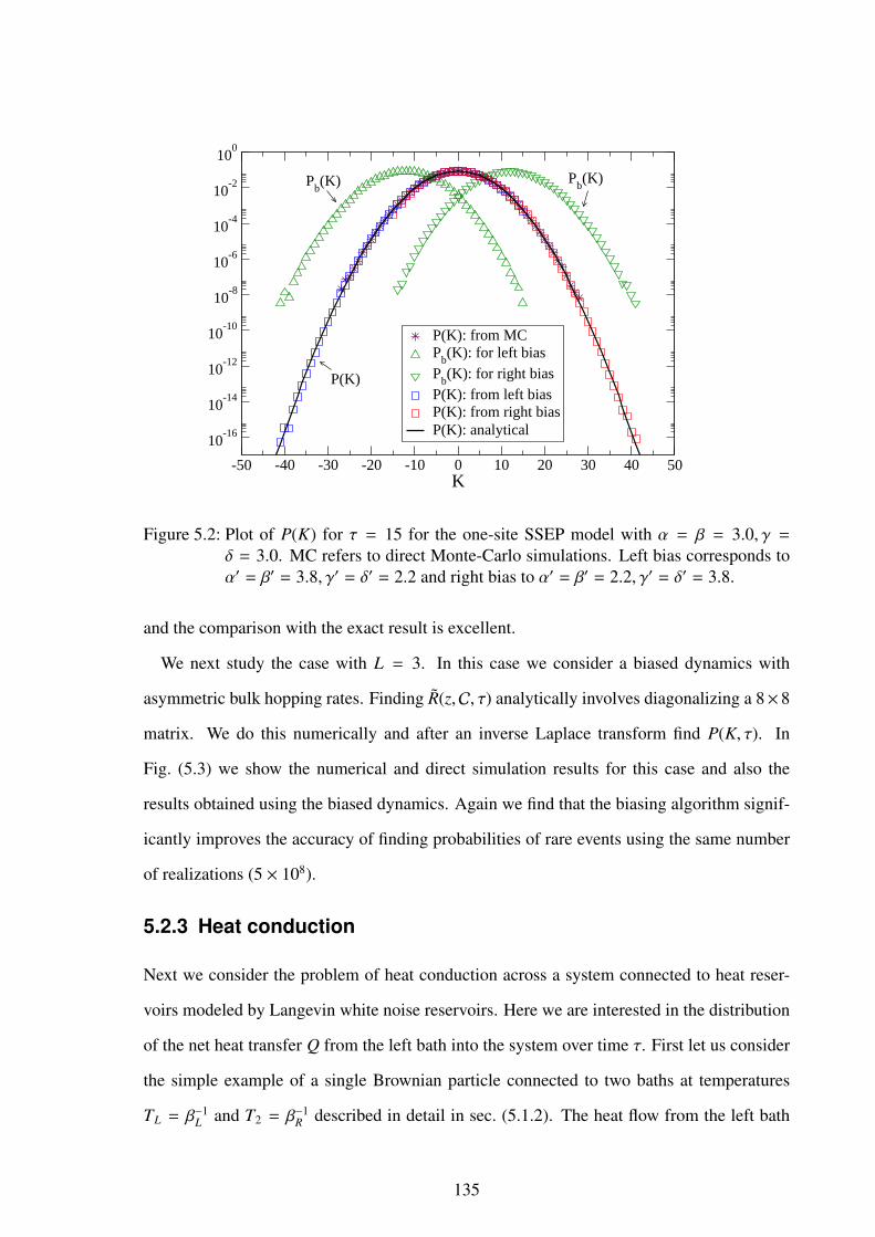
-50 -40 -30 -20 -10 0 10 20 30 40 50K
10-16
10-14
10-12
10-10
10-8
10-6
10-4
10-2
100
P(K): from MCP
b(K): for left bias
Pb(K): for right bias
P(K): from left biasP(K): from right biasP(K): analytical
Pb(K)P
b(K)
P(K)
Figure 5.2: Plot of P(K) for τ = 15 for the one-site SSEP model with α = β = 3.0, γ =δ = 3.0. MC refers to direct Monte-Carlo simulations. Left bias corresponds toα′ = β′ = 3.8, γ′ = δ′ = 2.2 and right bias to α′ = β′ = 2.2, γ′ = δ′ = 3.8.
and the comparison with the exact result is excellent.
We next study the case with L = 3. In this case we consider a biased dynamics with
asymmetric bulk hopping rates. Finding R(z,C, τ) analytically involves diagonalizing a 8×8
matrix. We do this numerically and after an inverse Laplace transform find P(K, τ). In
Fig. (5.3) we show the numerical and direct simulation results for this case and also the
results obtained using the biased dynamics. Again we find that the biasing algorithm signif-
icantly improves the accuracy of finding probabilities of rare events using the same number
of realizations (5 × 10⁸).
5.2.3 Heat conduction
Next we consider the problem of heat conduction across a system connected to heat reser-
voirs modeled by Langevin white noise reservoirs. Here we are interested in the distribution
of the net heat transfer Q from the left bath into the system over time τ. First let us consider
the simple example of a single Brownian particle connected to two baths at temperatures
TL = β−1L and T2 = β
−1R described in detail in sec. (5.1.2). The heat flow from the left bath
135

-20 -15 -10 -5 0 5 10 15 20 25 30K
10-20
10-18
10-16
10-14
10-12
10-10
10-8
10-6
10-4
10-2
100
P(K): from MCP
b(K): for left bias
Pb(K): for right bias
P(K): from left biasP(K): from right biasP(K): analytical
Pb(K) P
b(K)
P(K)
Figure 5.3: Plot of P(Q) for τ = 15 for the three-site SSEP model with α = β = 4.0, γ =δ = 2.0. MC refers to direct Monte-Carlo simulations. For left (right) biassimulations, the particles in bulk hop to the left (right) with rate 4 and to the right(left) with unit rate. The boundary rates are kept unchanged.
into the system in time τ is given by Q(τ) =∫ τ
0(−γLv2 +
√2DLηLv) dt. For the single Brow-
nian particle in this problem it is sufficient to specify the state by the velocity v(t) alone. If
we choose TL > TR then P(Q, τ) will have a peak at Q > 0. It is clear that in order to use
the biasing algorithm to compute probabilities of rare events with Q < 0 we can choose a
biased dynamics with temperatures of left and right reservoirs taken to be T ′L and T ′R with
T ′L < T ′R. The calculation of the weight factor W is somewhat tricky since computing P(v(t))
from P(ηL(t), ηR(t)) is non-trivial. Also one cannot eliminate ηL to express Q as a func-
tional of only the path v. To get around this problem we note the following mapping of the
single-particle system to the over-damped dynamics of two coupled oscillators given by the
equations of motion: x1 = −γ1(x1 − x2) +√
2DLηL , x2 = −γ2(x2 − x1) −√
2DRηR. The
variable x1 − x2 = x12 satisfies the same equation as v in Eq. (5.48). Thus with the same
definition for Q as given earlier we can use above equations for x1 and x2 to find P(Q, τ). In
this case we do not have the problem as earlier and both Q and W can be readily expressed
in terms of x1, x2. Let us denote by γ′i ,T′i ,D
′i the parameters of the biased system. Also
136

let η′L,R be the noise realizations in the biased process that result in the same path x1, x2 as
produced by ηL,R for the original process. Choosing Di = D′i for i = L,R it can be shown
that:
W =∫ τ
0dt [(η2
L/2 + η2R/2) − (η′2L /2 + η
′2R /2)]. (5.57)
Using the equations of motion we can express ηL,R, η′L,R in terms of the phase-space variables
and this gives:
W =1
4DL
∫ τ
0dt[2(γL − γ
′L)x1x12 + (γ2
L − γ′2L )x2
12]
+1
4DR
∫ τ
0dt[2(γR − γ
′R)x2x12 + (γ2
R − γ2R)x2
12],
Q =∫ τ
0dtx1x12.
Thus W and Q are easily evaluated in the simulation using the biased dynamics. In Fig. (5.4)
we show results for P(Q, τ) obtained both directly and using the biased dynamics. Again
we see that for the same number of realizations (109) one can obtain probabilities about
108 times smaller than using direct simulations. The comparison with the numerical results
obtained from the exact expression for 〈e−λQ〉 [109] also shows the accuracy of the algorithm.
It is easy to apply the algorithm to more complicated cases. For example consider a one-
dimensional chain of L particles connected to heat reservoirs at the two ends described by the
Langevin equations given in Eq. (5.2). The net heat transfer from left bath into the system
is given by Q =∫ τ
0(−γLv2
1 +√
2DLηLv1) and using Eqs. (5.2) this can be expressed in terms
of xl, vl as Q =∫ τ
0dtv1(m1v1 + (x1 − x2)). To apply our algorithm we consider a biased
dynamics where the Hamiltonian evolution is unchanged while the bath dynamics has new
parameters γ′L, γ′R,T
′L,T
′R which are chosen so that Pb(Q) has a peak in the required region.
Choosing D′i = Di we again find W by using Eqs. (5.2) in Eq. (5.57), as for the single particle
case. Thus both Q and W can be expressed in terms of the path and so are readily evaluated
for every realization of the biased dynamics.
As an example we study the case L = 2 with U = (x1 − x2)2/2 and with m1 = m2 = 1.
For the special parameters γL = γR =√
2 we use the results in [100] to obtain 〈e−λQ〉 ∼ eµ(λ)τ
137

-40 -30 -20 -10 0 10 20 30 40 50 60 70Q
10-16
10-14
10-12
10-10
10-8
10-6
10-4
10-2
100
P(Q): from MCP
b(Q): for left bias
P(Q): from left biasP(Q): analytical
P(Q)Pb(Q)
Figure 5.4: Plot of P(Q) for τ = 200 for heat conduction across a single free particle withγL = 0.8, γR = 0.2,TL = 1.1875,TR = 0.25. The parameters have been chosento correspond to a region in parameter-space where the fluctuation theorem isnot satisfied [109]. MC refers to direct Monte-Carlo simulations. The left biascorresponds to γ′L = γL, γ
′R = γ2/20,T ′L = TL,T ′R = 20TR.
-1200 -1000 -800 -600 -400 -200 0 200 400 600 800Q
10-12
10-10
10-8
10-6
10-4
10-2
P(Q): from MCP
b(Q): for left bias
Pb(Q): for right bias
P(Q): from left biasP(Q): from right biasP(Q): analytical
Pb(Q) P
b(Q)
P(Q)
Figure 5.5: Plot of P(Q) for τ = 100 for heat conduction across two particles connected by aharmonic spring with unit spring constant and γL = γR =
√2,TL = 10,TR = 12.
MC refers to direct Monte-Carlo simulations. The left bias corresponds to γ′L =γL, γ
′R = γR/2,T ′L = TL,T ′R = 2TR and right bias to γ′L = γL/2, γ′R = γR,T ′L =
2TL,T ′R = TR.
138

with µ(λ) =√
21− [1+ β−1
L β−1R λ(∆β − λ)]1/6 . This can be inverted to numerically compute
P(Q, τ) at large τ. In Fig. (5.5) we give the comparison between the analytical distribution
and that obtained by the biasing method.
5.3 Conclusions
We have calculated the large deviation function µ(λ) of the pdf of heat flow across a harmonic
chain. The large deviation function µ(λ) is expressed in terms of integration of a function
of the phonon transmission coefficient T (ω). Two cases, (a)single Brownian particle and
(b) two particles connected by harmonic spring were studied where for some special set of
parameters the integration in the expression for µ(λ) were carried out. For single Brownian
particle we also have obtained the steady state distribution.
We have presented an algorithm for computing the probabilities of rare events in various
nonequilibrium processes. The algorithm is an application of importance sampling and con-
sists in using a biased dynamics to generate the required rare events. The error in the estimate
of P(O, τ) is ≈ 〈e−2WδO,Ox〉1/2b /(MPb(O))1/2, and can be made small by choosing the biased
dynamics carefully. We have applied the algorithm to two different models of particle and
heat transport and shown that in both cases it gives excellent results. This algorithm is
straightforward to understand and also to implement.
5.4 Appendix
5.4.1 Expression of the matrix E(ω) :
Let us define vectors G1(ω) = iωe−iωε(G−111 (ω),−iG−1
11 (ω),G−11N(ω),−iG−1
1N(ω))T and Ψ =
(1,−i, 0, 0)T . In terms of these two vectors we can write ηL(ω) and v1(ω) (Eq. (5.32)) in
the following form :
ηL(ω) = ΨTξ(ω) = ξ(ω)Ψ
v1(ω) = GT1 (ω)ξ(ω) = ξ(ω)TG1(ω). (5.58)
139
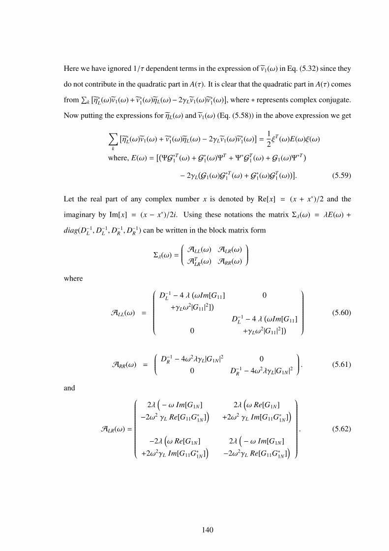
Here we have ignored 1/τ dependent terms in the expression of v1(ω) in Eq. (5.32) since they
do not contribute in the quadratic part in A(τ). It is clear that the quadratic part in A(τ) comes
from∑
k[η∗L(ω)v1(ω)+ v∗1(ω)ηL(ω)− 2γLv1(ω)v∗1(ω)
], where ∗ represents complex conjugate.
Now putting the expressions for ηL(ω) and v1(ω) (Eq. (5.58)) in the above expression we get
∑k
[η∗L(ω)v1(ω) + v∗1(ω)ηL(ω) − 2γLv1(ω)v∗1(ω)
]=
12ξT (ω)E(ω)ξ(ω)
where, E(ω) =[(ΨG∗T1 (ω) + G∗1(ω)ΨT + Ψ∗GT
1 (ω) + G1(ω)Ψ∗T)
− 2γL(G1(ω)G∗T1 (ω) + G∗1(ω)GT
1 (ω))]. (5.59)
Let the real part of any complex number x is denoted by Re[x] = (x + x∗)/2 and the
imaginary by Im[x] = (x − x∗)/2i. Using these notations the matrix Σλ(ω) = λE(ω) +
diag(D−1L ,D
−1L ,D
−1R ,D
−1R ) can be written in the block matrix form
Σλ(ω) =
ALL(ω) ALR(ω)
ATLR(ω) ARR(ω)
where
ALL(ω) =
D−1
L − 4 λ(ωIm[G11] 0
+γLω2|G11|
2])
D−1L − 4 λ
(ωIm[G11]
0 +γLω2|G11|
2])
(5.60)
ARR(ω) =
D−1R − 4ω2λγL|G1N |
2 0
0 D−1R − 4ω2λγL|G1N |
2
. (5.61)
and
ALR(ω) =
2λ(− ω Im[G1N] 2λ
(ω Re[G1N]
−2ω2 γL Re[G11G∗1N])
+2ω2 γL Im[G11G∗1N])
−2λ(ω Re[G1N] 2λ
(− ω Im[G1N]
+2ω2γL Im[G11G∗1N])
−2ω2γL Re[G11G∗1N])
. (5.62)
140

Similarly Σ−1λ (ω) can also be written in the following block matrix form
Σ−1λ (ω) =
1DLDRdetΣλ
ARR(ω) −ALR(ω)
−ATLR(ω) ALL(ω)
. (5.63)
5.4.2 Expressions of the elements of J(λ, ω) and c(ω) :
J1(λ, ω) = λ[g(ω) + g(−ω) − 2iωγLG11(ω)g(−ω) −G11(−ω)g(ω)
]+i
[eiωεg1(−ω) + e−iωεg1(ω)
],
J2(λ, ω) = iλ[g(ω) − g(−ω) + 2iωγLG11(ω)g(−ω) +G11(−ω)g(ω)
]−[eiωεg1(−ω) − e−iωεg1(ω)
], (5.64)
J3(λ, ω) = λ[− 2iωγLG1N(ω)g(−ω) −G1N(−ω)g(ω)
]+i
[eiωεg2(−ω) + e−iωεg2(ω)
],
J4(λ, ω) = iλ[2iωγLG1N(ω)g(−ω) +G1N(−ω)g(ω)
]−[eiωεg2(−ω) − e−iωεg2(ω)
],
and C(ω) =2λτγL|g(ω)|2. (5.65)
141

Bibliography
[1] N. W. Ashcroft and D. Mermin, Solid State Physics (Harcourt College Publishers,
1976).
[2] J. M. Ziman, Principles of the theory of solids (Second Edition, Cambridge University
Press, 1972).
[3] J. M. Ziman, Electrons and Phonons (Clarendon Press, Oxford, 1960).
[4] R. E. Peierls, Quantum Theory of Solids, (Oxford University Press, London, 1955).
[5] H. Spohn, J. Stat. Phys. 124, 1041, (2006).
[6] J. Lukkarinen and H. Spohn, Arch. Rat. Mech. Anal. 183, 93, (2007).
[7] J. M. Luttinger, Phys. Rev. 135, A1505, 1964
[8] C. Caroli, R. Combescot, P. Nozieres, and D. Saint-James, J. Phys. C 4 , 916, (1971).
[9] Y. Meir and N.S. Wingreen, Phys. Rev. Lett. 68, 2512, (1992).
[10] R. Landauer, Philos. Mag. 21, 863, (1970).
[11] Z. Rieder, J.L. Lebowitz, and E. Lieb, J. Math. Phys. 8, 1073, (1967).
[12] H. Nakazawa, Prog. Theor. Phys. 39, 236, (1968).
[13] D. Roy and A. Dhar, J. Stat. Phys. 131, 535, (2008).
[14] H. Matsuda and K. Ishii, Prog. Theor. Phys. Suppl. 45, 56, (1970).
142
[15] R.J. Rubin and W.L. Greer, J. Math. Phys. 12, 1686, (1971).
[16] T. Verheggen, Commun. Math. Phys. 68, 69, (1979).
[17] A. Casher and J.L. Lebowitz, J. Math. Phys. 12, 1701, (1971).
[18] M. Rich and W.M. Visscher, Phys. Rev. B 11, 2164, (1975).
[19] A. Dhar, Phys. Rev. Lett. 86,5882, (2001).
[20] N. Likhachev et al., Phys. Rev. E 73,016701, (2006).
[21] A. Dhar and J.L. Lebowitz, Phys. Rev. Lett. 100,134301, (2008).
[22] D. Roy and A. Dhar, Phys. Rev. E 78, 051112, (2008).
[23] M. Bolsterli, M. Rich, and W.M. Visscher, Phys. Rev. A 4, 1086, (1970).
[24] Dhar and D. Roy, J. Stat. Phys. 125, 801, (2006).
[25] S. John, H. Sompolinsky, and M.J. Stephen, Phys. Rev. B 27, 5592, (1983).
[26] L. Yang, Phys. Rev. Lett. 88, 094301, (2002).
[27] L.W. Lee and A. Dhar, Phys. Rev. Lett. 95, 094302, (2005).
[28] O. Narayan and S. Ramaswamy, Phys. Rev. Lett. 89, 200601, (2002).
[29] S. Lepri, R. Livi, and A. Politi, Europhys. Lett. 43, 271, (1998).
[30] S. Lepri, Phys. Rev. E 58 (1998), p. 7165.
[31] L. Delfini, S. Lepri, R. Livi, and A. Politi, J. Stat. Mech. (2007).
[32] J.S. Wang and B. Li, Phys. Rev. Lett. 92, 074302, (2004).
[33] J.S. Wang and B. Li, Phys. Rev. E 70, 021204, (2004).
[34] S. Lepri, R. Livi, and A. Politi, Phys. Rev. E 68, 067102, (2003).
143

[35] K. Aoki and D. Kusnezov, Phys. Rev. Lett. 86, 4029, (2001).
[36] T. Mai, A. Dhar, and O. Narayan, Phys. Rev. Lett. 98, 184301, (2007).
[37] A. Dhar and K. Saito, Phys. Rev. E vol. 78, 061136 (2008).
[38] C. Giardina, R. Livi, A. Politi, and M. Vassalli, Phys. Rev. Lett. 84, 2144, (2000).
[39] B. Li, H. Zhao, and B. Hu, Phys. Rev. Lett. 86, 63, (2001).
[40] A. Dhar and K. Saito, Phys. Rev. E 78, 061136 (2008).
[41] G. Casati, Found. Phys. 16, 51, (1986).
[42] T. Hatano, Phys. Rev. E 59, R1, (1999).
[43] P.L. Garrido, P.I. Hurtado, and B. Nadrowski, Phys. Rev. Lett. 86, 5486, (2001).
[44] A. Dhar, Phys. Rev. Lett. 86, 3554, (2001).
[45] P. Grassberger, W. Nadler, and L. Yang, Phys. Rev. Lett. 89, 180601, (2002).
[46] A.V. Savin, G.P. Tsironis, and A.V. Zolotaryuk, Phys. Rev. Lett. 88,154301, (2002).
[47] G. Casati and T. Prosen, Phys. Rev. E 67, 015203, (2003).
[48] G. Casati, J. Ford, F. Vivaldi, and W.M. Visscher, Phys. Rev. Lett. 52, 1861, (1984).
[49] T. Prosen and M. Robnik, J. Phys. A: Math. Gen. 25, 3449, (1992).
[50] B. Hu, B. Li, and H. Zhao, Phys. Rev. E 57, 2992, (1998).
[51] K. Aoki and D. Kusnezov, Phys. Lett. A 265, 250, (2000).
[52] K. Aoki and D. Kusnezov, Ann. Phys. (N.Y.) 295, 50, (2002).
[53] A. Lippi and R. Livi, J. Stat. Phys. 100, 1147, (2000).
[54] L. Yang, P. Grassberger, and B. Hu, Phys. Rev. E 74, 062101, (2006).
144

[55] H. Shiba and N. Ito, J. Phys. Soc. Jpn 77, 054006, (2008).
[56] T. Shimada, T. Murakami, S. Yukawa, K. Saito, and N. Ito, J. Phys. Soc. Jpn 69, 3150,
(2000).
[57] K. Saito and A. Dhar, Phys. Rev. Lett. 104, 040601, (2010).
[58] A. Dhar, Advances in Physics, 57, 457, (2008).
[59] S. Lepri, R. Livi, and A. Politi, Phys. Rep. 377, 1, (2003).
[60] G. W. Ford, M. Kac and P. Mazur, J. Math. Phys. 6, 504, (1965).
[61] A. Dhar and B. S. Shastry, Phys. Rev. B 67, 195405, (2003).
[62] A. Dhar and D. Sen, Phys. Rev. B 73, 085119, (2006).
[63] Unpublished notes of Dr. Abhishek Dhar
[64] S. Datta, Electronic transport in mesoscopic systems (Cambridge University Press,
1995)
[65] L. G. C. Rego and G. Kirczenow, Phys. Rev. Lett. 81, 232, (1998).
[66] M. P. Blencowe, Phys. Rev. B 59, 4992, (1999).
[67] T. Yamamoto and K. Watanabe, Phys. Rev. Lett. 96, 255503, (2006).
[68] J. S. Wang, J. Wang and N. Zeng, Phys. Rev. B 74, 033408, (2006).
[69] A. J. O’Connor and J. L. Lebowitz, J. Math. Phys. 15, 692, (1974).
[70] P. W. Anderson, Phys. Rev. 109, 1492, (1958).
[71] I. Savic, N. Mingo and D. A. Stewart, Phys. Rev. Lett. 101, 165502, (2008).
[72] G. Stoltz, M. Lazzeri and F. Mauri, Jn. Phys. Cond. Matt. 21 245302, (2009).
[73] N. F. Mott and W. D. Twose, Adv. Phys. 10, 107, (1961).
145

[74] R. E. Borland, Proc. R. Soc. London, Ser. A 274, 529, (1963).
[75] I. Ya. Goldsheid, S. A. Molchanov and L. A. Pastur, Funct. Anal. Appl. 11, 1, (1977).
[76] P. A. Lee and T. V. Ramakrishnan, Rev. Mod. Phys. 57, 287, (1985).
[77] J. Callaway, Phys. Rev. 113, 1046, (1959).
[78] P. B. Allen and J. L. Feldman, Phys. Rev. Lett. 62, 645, (1989).
[79] N. Xu et al., Phys. Rev. Lett. 102, 038001, (2009).
[80] D. N. Payton and W. M. Visscher, Phys. Rev. 154, 802, (1967).
[81] P. Dean, Rev. Mod. Phys. 44, 127, (1972).
[82] A. Kundu, A. Chaudhuri and A. Dhar, to be published.
[83] G. Basile, C. Bernardin, S. Olla, Phys. Rev. Lett. 96, 204303 (2006).
[84] M. S. Green, J. Chem. Phys. 22, 398, (1954).
[85] R. Kubo, M. Yokota, and S. Nakajima, J. Phys. Soc. Jpn. 12, 1203, (1957);
[86] H. Mori, Phys. Rev. 112, 1829 (1958); M. S. Green, Phys. Rev. 119, 829 (1960); L.P
Kadanoff and P. C. Martin, Annals of Physics 24, 419 (1963); J. M. Luttinger, Phys.
Rev. 135, A1505, (1964); W. M. Visscher, Phys. Rev. A. 10, 2461 (1974).
[87] K. R. Allen and J. Ford, Phys. Rev. 176, 1046 (1968).
[88] D. S. Fisher and P. A. Lee, Phys. Rev. B 23, 6851 (1981).
[89] G. Gallavotti, Phys. Rev. Lett. 77, 4334 (1996).
[90] J.L. Lebowitz and H. Spohn, J. Stat. Phys. 95, 333 (1999).
[91] L. Rey-Bellet and L. E. Thomas, Annales Henri Poincare 3, 483 (2002); L. Rey-Bellet,
in: XIVth International Congress on Mathematical Physics, World Sci. Publ., Hacken-
sack, NJ, 2005 pp. 447-454.
146

[92] D. Andrieux and P. Gaspard, J. Stat. Mech. P02006, (2007).
[93] H. Haken, Rev. Mod. Phys. 47, 67 (1975).
[94] H. Risken, The Fokker-Planck Equation: Methods of solutions and applications,
Springer-Verlag Berlin Heidelberg, Second Edition, 1989.
[95] J. Kurchan, arxiv:0901.1271.
[96] E. A. Novikov, Zh. Eksp. Teor. Fiz. 47, 1919 (1964); Sov. Phys. JETP 20, 1290 (1965);
V. V. Konotop and L. Vazquez, Nonlinear Random Waves, WorldScientific (Singapore)
1994, pp 14-15..
[97] P. Mazur and E Montroll, J. Math. Phys. 1, no.1, (1960).
[98] D. W. Jepsen, J. Math. Phys. 6, no.3, (1965).
[99] W. A. M. Morgado and D. O. Soares-Pinto, Phys. Rev. E 79 (2009) 051116.
[100] K. Saito, A. Dhar, Phys. Rev. Lett. 99, 180601 (2007).
[101] R. Rubin and W. Greer, J. Math. Phys. (N.Y.) 12, 1686 (1971).
[102] T. Verheggen, Commun. Math. Phys. 68, 69, (1979).
[103] M. Rich and W. M. Visscher, Phys. Rev. B 11, 2164, (1975).
[104] D. J. Evans, E. G. D. Cohen, and G. P. Morriss, Phys. Rev. Lett. 71, 2401 (1993);
D. J. Evans and D. J. Searles, Phys. Rev. E 50, 1645 (1994); G. Gallavotti and E.G.D.
Cohen, Phys. Rev. Lett. 74, 2694 (1995); J. L. Lebowitz and H. Spohn, J. Stat. Phys.
95, 333 (1999);
[105] C. Jarzynski and D. K. Wojcik, Phys. Rev. Lett. 92, 230602 (2004).
[106] T. Bodineau, B. Derrida, Phys. Rev. Lett. 92, 180601 (2004); C. Enaud, B. Derrida, J.
Stat. Phys. 114, 537 (2004).
147

[107] B. Derrida, B. Doucot and P.-E. Roche J. Stat. Phys. 115, 717-748 (2004).
[108] B. Derrida, J.L. Lebowitz, Phys. Rev. Lett. 80, 209 (1998).
[109] P. Visco, J. Stat. Mech. P06006 (2006).
[110] C. Jarzynski, Phys. Rev. Lett. 78, 2690 (1997); G. E. Crooks, Phys. Rev. E 60, 2721
(1999); T. Hatano and S. Sasa, Phys. Rev. Lett. 86, 3463 (2001); U. Seifert, Phys. rev.
lett. 95, 040602, (2005).
[111] C. Giardina, J. Kurchan and L. Peliti, Phys. Rev. Lett. 96, 120603 (2006)
[112] P. I. Hurtado and P. L. Garrido, Phys. Rev. Lett. 102, 250601 (2009); J. Stat. Mech.
(2009) P02032.
[113] O. Mazonka, C. Jarzyski and J. Bocki, Nucl. Phys. A 641, 335 (1998).
[114] C. Dellago, P. G. Bolhuis, F. S. Csajka, and D. Chandler, J. Chem. Phys. 108, 1964
(1998).
[115] R. J. Allen, P. B. Warren, and P. R. ten Wolde, Phys. Rev. Lett. 94, 018104 (2005).
[116] H. Touchette, Phys. Rep. 478, 1 (2009).
[117] J. Farago, J. Stat. Phys., 107, 781 (2002).
[118] R. van Zon and E. G. D. Cohen, Phys. Rev. Lett. 91, 110601 (2003); ibid. Phys. Rev.
E 69, 056121 (2004).
[119] J. Kurchan, J. Phys. A: Math. Gen. 31, 3719 (1998)
[120] F. van Wijland, Phys. Rev. E 74, 063101 (2006).
[121] Details will be published elsewhere.
148