Differentiated Surveillance for Sensor NetworksTing Yan Tian He John A. Stankovic

Department of Computer Science, School of Engineering, University of Virginia

151 Engineer’s Way, P.O.Box 400740, Charlottesville, Virginia 22904-4740, USA

{ty4k, tianhe, stankovic}@cs.virginia.edu

ABSTRACTFor many sensor network applications such as military surveillance, it is necessary to provide full sensing coverage to a security-sensitive area while at the same time minimizing energy consumption and extending system lifetime by leveraging the redundant deployment of sensor nodes. It is also preferable for the sensor network to provide differentiated surveillance service for various target areas with different degrees of security requirements. In this paper, we propose a differentiated surveillance service for sensor networks based on an adaptable energy-efficient sensing coverage protocol. In the protocol, each node is able to dynamically decide a schedule for itself to guarantee a certain degree of coverage (DOC) with average energy consumption inversely proportional to the node density. Several optimizations and extensions are proposed to provide even better performance. Simulation shows that our protocol accomplishes differentiated surveillance with low energy consumption. It outperforms other state-of-the-art schemes by as much as 50% reduction in energy consumption and as much as 130% increase in the half-life of the network.

Categories and Subject DescriptorsC.2. [Computer Communication Networks]: Network Protocols

General TermsAlgorithms, Performance, Design

KeywordsSensor Networks, Sensing Coverage, Energy Conservation, Differentiated Service

1. INTRODUCTIONWireless Sensor Networks have emerged as a new information-gathering paradigm based on the collaborative effort of a large

number of sensing nodes. In such networks, nodes deployed in a remote environment must self-configure without any a priori information about the network topology or global view. Nodes act in response to environmental events and relay collected and possibly aggregated information through the dynamically formed multi-hop wireless network in accordance with desired system functionality. These networks can form the basis for many types of smart environments such as smart hospitals, battlefields, earthquake response systems, and learning environments. A set of applications, such as biomedicine, hazardous environment exploration, environmental monitoring, military tracking and reconnaissance surveillance are the key motivations for many recent research efforts in this area.

Low-cost deployment is one acclaimed advantage of sensor networks, which imply that the resources available to individual nodes are severely limited. Limited processor bandwidth and small memory are two arguable constraints in sensor networks, which will disappear with the development of fabrication techniques. However, the energy constraint is unlikely to be relieved quickly due to slow progress in developing battery capacity. Moreover, the untended nature of sensor nodes and hazardous sensing environments preclude battery replacement as a feasible solution. On the other hand, the surveillance nature of sensor network applications requires a long lifetime; therefore, it is a very important research issue to provide a form of energy-efficient surveillance service for a geographic area.

Previous research focuses on how to provide full or partial sensing coverage in the context of energy conservation. In such an approach, nodes are put into a dormant state as long as their neighbors can provide sensing coverage for them. These solutions regard the sensing coverage to a certain geographic area as binary, either it provides coverage or not. However, we argue that, in most scenarios such as battlefields, there are certain geographic sections such as the general command center that are much more security-sensitive than others. Based on the fact that individual sensor nodes are not reliable and subject to failure and single sensing readings can be easily distorted by background noise and cause false alarms, it is simply not sufficient to rely on a single sensor to safeguard a critical area. In this case, it is desired to provide higher degree of coverage in which multiple sensors monitor the same location at the same time in order to obtain high confidence in detection. On the other hand, it is overkill and energy consuming to support the same high degree of coverage for some non-critical area. Based on such observations, this paper leverages previous solutions and addresses the problem of providing a differentiated surveillance service for sensor networks. By differentiated

Permission to make digital or hard copies of all or part of this work for personal or classroom use is granted without fee provided that copies are not made or distributed for profit or commercial advantage and that copies bear this notice and the full citation on the first page. To copy otherwise, or republish, to post on servers or to redistribute to lists, requires prior specific permission and/or a fee.

SenSys’03, November 5–7, 2003, Los Angeles, California, USA.

Copyright 2003 ACM 1-58113-707-9/03/0011…$5.00

surveillance, we mean providing different degrees of sensing coverage for a sensor network according to different requirements. Two major goals are achieved in this paper. First, our new sensing coverage algorithm outperforms other state-of-the-art solutions in terms of energy conservation, energy balance and communication overhead when it runs in non-differentiated mode. Second, this paper is the first to propose differentiated surveillance for sensor networks with minimal overhead.

The remainder of the paper is organized as follows: Section 2 discusses previous research related to the sensing coverage problem found in sensor networks. Section 3 describes the design of our sensing coverage protocol without differentiation. Section 4 extends the design to provide differentiated surveillance. Section 5 gives a brief description of baselines to which we compare our work, including two other state-of-the-art sensing coverage protocols. Section 6 provides a detailed performance evaluation and comparison. We conclude the paper in Section 7.

2. RELATED WORKA set of research issues needs to be addressed before surveillance-based applications such as military tracking and environmental monitoring become technically feasible and economically practical. Recently, several schemes are proposed to address the sensing coverage problem in sensor networks. In [18], full surveillance coverage is support by a node-scheduling scheme based on off-duty eligibility rules, which allows nodes to turn themselves off as long as the neighboring nodes can cover the area for them. This rule guarantees 100% sensing coverage as long as no void exists. However, this rule underestimates the area that the neighbor nodes can cover, which leads to excess energy consumption. In [22], surveillance coverage is achieved by a probing mechanism. In this solution, after a sleeping node wakes up, it broadcasts a probing message within a certain range and waits for a reply. If no rely is received within a timeout, it will take the responsibility of surveillance until it depletes its energy. In this solution, the probing range and wakeup rate can be adjusted to affect the degree of coverage indirectly. However, this probing-based approach has no guarantee on sensing coverage and blind points can occur. Our solution is different from these solutions in the sense that it can not only guarantee sensing coverage to a certain geographic area, but it can also adapt the degree of coverage to that area, up to the limitation imposed by the number of sensor nodes present.

Energy balancing is another research issue addressed in this paper. [18] and [22] only consider the metric in terms of the total amount of energy consumed regardless of the distribution of the energy among the nodes. We argue that unbalanced energy dissipation causes some nodes to die much faster than others do, therefore, the half-life of the network is dramatically reduced in the un-balanced approach. Research has addressed the energy balance issue from different aspects of sensor networks. SPEED [10] balances the traffic by non-deterministically forwarding the packet through multiple routes. GAF [20] performs leader rotation among the nodes inside a virtual grid, in order to balance energy consumption.

Research on network topology control such as SPAN [4], LEACH [10] and GAF [20] addresses the problem of providing

communication coverage within an energy conservation context. These have a similar flavor as the surveillance coverage problem. For example, LEACH [10] partitions a network into clusters and randomly rotates the cluster leader in order to evenly distribute the energy consumption among the sensors. SPAN [4] is another randomized algorithm where nodes make local decisions on whether to sleep or to join a backbone network in order to reduce energy consumption. The major difference between those and this work is that communication coverage considers only connectivity between the nodes. In contrast, surveillance (sensing) coverage addresses the coverage problem to every physical point in the terrain. As a result, new scheduling is required to force some nodes stay awake for surveillance purposes even though they are not participating in data forwarding.

Besides the aforementioned work in communication and sensing coverage that conserves energy, work in energy conservation for general sensor networks has been considered at various levels of the communication stack. From the bottom to the top, special hardware [15] is designed with multiple energy dissipation settings. MAC layer protocols developed for energy savings mostly take advantage of overhearing and scheduling to allow nodes to sleep while they are not transmitting or receiving messages [7][11]. At the network and routing layers, solutions are diversified. Data placement schemes [3] minimize energy along the transmission path through data caching. In [16], R. Ramanathan et. al. adjust communication range dynamically based on the node density to conserve energy consumed in transmission. MFR [17] by Takagi et. al. uses a minimal hop path to reduce the total number of transmissions. [21] sets routes according to the energy remaining at nodes along that path, and [10] uses mechanisms to save energy through the distribution of messages among various paths from source to destination. At the application layer, the protocols incorporate routing semantics to form groups and rotate leadership responsibilities, allowing non-leader nodes to sleep and conserve their energy [4]. Finally, data aggregation techniques inside the network and application layers also provide energy conservation features in both application independent [8] and application dependent fashions [12][13]. All of these protocols tackle the energy issue from different aspects of sensor networks, thus we consider them complementary to our work.

Recently, research has started to address QoS issues to support differentiated services for sensor networks. SWAN [1] uses feedback information from the MAC layer to regulate the transmission rate of non-real-time traffic in order to sustain real-time traffic. RAP [14] uses velocity monotonic scheduling to prioritize real-time traffic and enforces such prioritization through a differentiated MAC Layer. In [2], the delivery ratios of packets at different priority levels are affected by the forwarding probability at intermediate nodes. To date, to the best of our knowledge, no algorithm has been specifically designed to address how to provide differentiated surveillance for sensor networks. Due to the surveillance nature of most sensor network applications, we deem that this service is essential.

3. BASIC PROTOCOL DESIGNIn this section and section 4, we introduce the design of an adaptive sensing coverage scheme for sensor networks. The basic design without differentiation is introduced first in section 3. This is then the basis for the extension for differentiated surveillance to support scenarios in which a partial coverage (<100%) is sufficient or a high degree of coverage (>100%) is desired (section 4).

3.1 Design GoalsThe basic design goal for this work is to provide energy efficient sensing coverage for a geographic area covered by sensor nodes. Though it has been addressed in previous work [18] [22], our work distinguishes itself from previous solutions in following sub-goals that we achieve.

Reduce total amount of energy consumed.

Reduce energy variation among nodes.

Reduce communication overhead in establishing nodes’ work schedules.

Support a new extension to the service for differentiated surveillance with small overhead.

Provide communication connectivity as an auxiliary benefit.

In the remaining parts of the paper, we support these claims with analytical analysis and simulation results.

3.2 AssumptionsFirst, we assume that each node knows its own location [9] and nodes are not moving. The node location information does not need to be precise when we are using conservative sensing ranges to decide the schedules (see 3.4). These are common assumptions for many sensor network applications. For simplicity and convenience of protocol description in the rest of the paper, we refer to the sensing area of a node as a circle with a nominal radius r centered at the location of the node itself. We will later show that we can also deal with irregular and/or non-uniform sensing areas as long as the neighboring nodes are aware of each other’s sensing area. In the protocol description, we deploy the sensor nodes in a two-dimensional Euclidean plane. However, the protocol can be extended to a three-dimensional space or a curved surface without much difficulty. We also assume that the neighboring nodes should be roughly time synchronized on the order of seconds, which can be easily achieved by current millisecond-level synchronization solutions such as found in [6]. Also, the tolerance for small synchronization skews (see 3.4.2) allows the re-synchronization process to happen even less frequently so that the cost can be neglected.

The last assumption we make is that nodes can directly communicate with the neighboring nodes within a radius larger than 2r (r is nominal sensing radius). This is a typical case in all systems we experienced. For example, MICA II [5] has a communication range of about 1000 feet, while the sensing range is within a hundred feet even with long-range motion sensors. Actually, this is an optional assumption. The protocol works so long as the nodes are able to communicate directly or indirectly with each other within the distance of 2r and the communication range need not be regular. We make this

assumption for simplicity in the protocol description and to avoid routing overhead for any two nodes that can sense a common area. This assumption also helps provide a connectivity guarantee when full sensing coverage is achieved.

3.3 Basic Design without DifferentiationEach node in the sensor network is either in sleeping mode or in working mode. Our goal for the basic design without differentiation is to have as many nodes as possible go to sleep to save energy and extend the lifetime of the sensor network while guaranteeing 100% sensing coverage to the target area.

3.3.1 A Node’s Working ScheduleThe lifetime of a sensor network is composed of an initialization phase and a sensing phase. During the initialization phase, each sensor node finds its own position [9] and synchronizes [6] time with neighboring nodes. After that, nodes enter into a sensing phase and start to sense environmental events. The sensing phase of nodes is divided into rounds with equal duration and are synchronized. Each node will establish a working schedule through our algorithm, which tells it when to sleep and when to work for each round. When a node goes to sleep, its sensing, communication and computation components can all be asleep and only a timer needs to work and wake up all components according to its schedule.

We denote the duration of each round as T. The schedule for a node is determined by a tuple with four parameters: (T, Ref, Tfront, Tend). As shown in Figure 1, Ref is a random time reference point chosen by a node within [0, T). Tfront is the duration of time prior to the reference point Ref and Tend is the duration of time after reference point Ref. We describe how to decide these parameters in section 3.3.2. For any given tuple (T, Ref, Tfront, Tend), a node executes the following working schedule:

A node wakes up at time (T × i + Ref – Tfront) and goes to sleep at time (T × i + Ref + Tend)

Figure 1. Node Working ScheduleIt should be noted that the following two rules hold for the schedule:

1) The tuple (T, Ref, Tfront, Tend) for each node is chosen during the initialization phase and does not change during the whole sensing phase, unless rescheduling is required for fault-tolerance purposes.

2) Time duration Tfront and Tend should be in the interval [0, T) and furthermore, the sum of Tfront and Tend, which is the time duration for a node to work during each round, should be less than or equal to T.

3.3.2 Setting Tuple Parameters (T, Ref, Tfront, Tend)In our approach, we cover the target area with a virtual square grid. We describe how to choose the unit grid size later in section 3.4.1. Now we describe the protocol that decides the schedule for each sensor node to guarantee that each grid point in the target area is covered by at least one working node at any time and with minimum energy consumption. Here we only consider the energy consumed by the sensing function, so the energy consumed by a node is proportional to its working time for each round, which is (Tfront + Tend). Parameter T, which is the duration of each round, is pre-determined and kept constant across all the nodes inside the sensor network. We discuss how to set this parameter in more detail in section 3.4.2.

Figure 2. Sensing Coverage to Single Grid Point XAfter the nodes complete localization and time synchronization, they each broadcast a beacon (a random jitter in transmission time is added to avoid collision). This beacon has the information of its location and a randomly chosen time reference point Ref. The reference time should be uniformly chosen among [0, T) and follows an identical independent distribution (iid). According to the assumption of direct communication within 2r, each node within the distance of 2r of the sending node should receive the beacon. For example in Figure 2, nodes A, B and C will hear each other. After every node beacons the time reference point Ref, each node maintains a neighbor table with the information of locations and time reference points of its neighbors within 2r’s distance. For example, node A will keep information about nodes B, C and itself in a table. D’s beacon is ignored since it is outside the 2r’s distance of A.

Before discussing the sensing coverage of the entire area, we first focus on how to provide sensing coverage for a single grid point. Here we consider node A and grid point x shown in Figure 2. Obviously, all the sensor nodes whose sensing areas cover grid point x are in the 2r’s distance of node A. Therefore, node A has the information of their locations and time reference points in its neighbor table. With such information node A sorts those time reference points in ascending order and lays out all N reference times including its own reference time point (see Figure 3). (Suppose that the total number of sensor nodes which can cover grid point x is N).

Without loss of generality, suppose node A has the ith reference time Ref(i), node B has the (i-1)th reference time Ref(i-1) and node C has the (i+1)th reference time Ref(i+1). Then the time interval Tfront and the time interval Tend for grid point x are set by our algorithm to [Ref(i) - Ref(i-1)]/2 to [Ref(i+1) - Ref(i)]/2,

respectively. There are two special cases for the Tend and Tfront

calculations:

1) If node A has the smallest reference time among all N nodes that can cover grid point X, then the time interval Tfront is (T+ Ref(1)-Ref(n))/2 and the time interval Tend is (Ref(2)-Ref(1))/2.

2) If node A has the largest reference time among all N nodes that can cover grid point X, then the time interval Tfront is (Ref(n)-Ref(n-1))/2 and the time interval Tend is (T+ Ref(1)-Ref(n))/2.

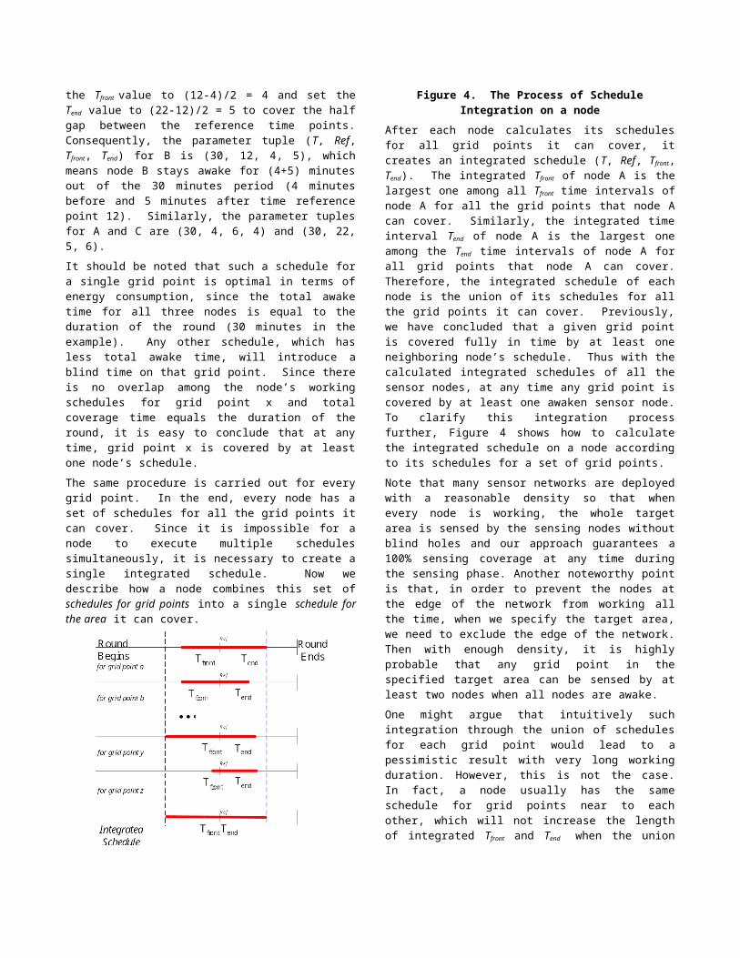
Figure 3. Calculating node schedules for a single grid pointTo understand the procedure better, we explain how to decide node schedules for a certain grid point x through an example shown in Figure 3. Suppose the duration of each round T is 30 minutes and only nodes A, B and C can provide coverage to grid point x. Nodes A, B and C choose reference time Ref values 4, 12 and 22, respectively. According to our algorithm, node B will set the Tfront value to (12-4)/2 = 4 and set the Tend value to (22-12)/2 = 5 to cover the half gap between the reference time points. Consequently, the parameter tuple (T, Ref, Tfront, Tend) for B is (30, 12, 4, 5), which means node B stays awake for (4+5) minutes out of the 30 minutes period (4 minutes before and 5 minutes after time reference point 12). Similarly, the parameter tuples for A and C are (30, 4, 6, 4) and (30, 22, 5, 6).

It should be noted that such a schedule for a single grid point is optimal in terms of energy consumption, since the total awake time for all three nodes is equal to the duration of the round (30 minutes in the example). Any other schedule, which has less total awake time, will introduce a blind time on that grid point. Since there is no overlap among the node’s working schedules for grid point x and total coverage time equals the duration of the round, it is easy to conclude that at any time, grid point x is covered by at least one node’s schedule.

The same procedure is carried out for every grid point. In the end, every node has a set of schedules for all the grid points it can cover. Since it is impossible for a node to execute multiple schedules simultaneously, it is necessary to create a single integrated schedule. Now we describe how a node combines this set of schedules for grid points into a single schedule for the area it can cover.

Figure 4. The Process of Schedule Integration on a nodeAfter each node calculates its schedules for all grid points it can cover, it creates an integrated schedule (T, Ref, Tfront, Tend). The integrated Tfront of node A is the largest one among all Tfront time intervals of node A for all the grid points that node A can cover. Similarly, the integrated time interval Tend of node A is the largest one among the Tend time intervals of node A for all grid points that node A can cover. Therefore, the integrated schedule of each node is the union of its schedules for all the grid points it can cover. Previously, we have concluded that a given grid point is covered fully in time by at least one neighboring node’s schedule. Thus with the calculated integrated schedules of all the sensor nodes, at any time any grid point is covered by at least one awaken sensor node. To clarify this integration process further, Figure 4 shows how to calculate the integrated schedule on a node according to its schedules for a set of grid points.

Note that many sensor networks are deployed with a reasonable density so that when every node is working, the whole target area is sensed by the sensing nodes without blind holes and our approach guarantees a 100% sensing coverage at any time during the sensing phase. Another noteworthy point is that, in order to prevent the nodes at the edge of the network from working all the time, when we specify the target area, we need to exclude the edge of the network. Then with enough density, it is highly probable that any grid point in the specified target area can be sensed by at least two nodes when all nodes are awake.

One might argue that intuitively such integration through the union of schedules for each grid point would lead to a pessimistic result with very long working duration. However, this is not the case. In fact, a node usually has the same schedule for grid points near to each other, which will not increase the length of integrated Tfront and Tend when the union operation takes place. This has been shown in the simulation.

Our approach has several major advantages for sensor network deployment:

1) Communication overhead in our approach is minimized. For the approach described above, each node needs only to beacon one message without consideration of collisions.

Compared to approaches that a node beacons each time it wakes up [22] or for each round [18], the energy consumed by our approach’s communication is much less.

2) The random time reference point with uniform distribution contributes to the energy balance among the nodes. An optimization on this (discussed later) can enhance this energy-balancing feature even more.

3) Due to the optimal energy consumption property for a single grid point1, the total energy consumption of our approach increases very slowly with the increase of node density. As a result, the system lifetime increases proportionally with the increase in node density. We show this in the evaluation section.

Although the length of working time for each node may differ due to randomness, the protocol is still fair in the sense that no node is given priority to work longer or shorter.

It can be easily seen from the above description that even when at the initialization phase some node is not discovered by its neighbors, once there are enough nodes to cover the target area, the 100% sensing coverage is still guaranteed. However, it may cause other nodes to work unnecessarily longer.

The protocol just described provides a guarantee of 100% sensing coverage at any time for the target area. Acknowledging that in some situations, full coverage by single sensor nodes is not enough to obtain high confidence in detection, our basic design can be easily extended to provide a guaranteed degree of coverage for a geographic area with very small overhead (see section 4).

3.4 Design IssuesThis section completes our approach with several design issues concerning grid granularity, clock skew, irregular sensing patterns and node failures.

3.4.1 Dealing with Possible Blind Points in Space due to the Large Granularity of the Grid SizeOne may argue that in our protocol description, there can be small sensing holes because we only guarantee grid point coverage, instead of a grid area. Here we will explain why this approach still makes sense. We denote the unit grid size as d. We also define a conservative sensing area of a sensor node as a smaller concentric circle than its actual sensing area in order to handle this problem and other issues.

d

d 2

actual

conservative

Figure 5. Grid Size Granularity Issues

1 However, the integrated schedule is sub-optimal due to working schedule redundancy among nodes.

From figure 5, it can be easily seen that the target area is fully covered by the sensor nodes' actual sensing areas as long as 1) each grid point is inside the conservative sensing area of at least one sensor node, and 2) the difference between the actual sensing radius and the conservative sensing radius

is greater than . Then the problem of covering the whole target area with actual sensing areas reduces to that of covering the grid points with conservative sensing areas. With such observations, we decide the upper bound of the grid size according to the following rules.

1) If we use the actual sensing radius to calculate the nodes’ working schedules, the grid size d should be smaller than the size of the objects we want to detect, so that these objects will not fit in the gap among the grid points.

2) If we use a conservative sensing radius, the grid size d should be smaller than .

At the same time, a lower bound for the grid size should be set with consideration of computational cost (see 3.7.1).

Other factors like the imprecision of location information and irregularity of the sensing areas should also be considered when we decide the conservative sensing radius.

In the remaining protocol description, we do not distinguish between concepts of grid point coverage and area coverage.

3.4.2 Dealing with Possible Blind Points in Time due to Synchronization SkewDue to the precision limits of synchronization algorithms for real sensor network systems, there is always some synchronization skew. When nodes try to trigger some events at the same time, the actual time the event is triggered on each node will be different due to the synchronization skew. Our protocol is based on synchronization, so we must compensate for the synchronization skew to make the schedules seamless. We define the maximum skew of the whole sensor network as Ts. In order to bridge the gaps caused by the synchronization skew, we only need to extend the schedule of each node for Ts/2 in both directions. This compensation affects the performance of the protocol. In order to minimize the impact of this performance degradation, it is favorable to increase the time duration T for each round. The reason is that when Ts is fixed, the longer a round is, the lower is the compensation overhead compared to the duration of a round or the schedules for a round. For example, suppose Tfront+Tend is 30 minutes, if we allow synchronization skew to be 1 second, the performance will be degraded less than 0.1%. However, T should not be very large, which may lead to unbalanced energy consumption.

3.4.3 Dealing with Possible Blind Points in Space due to Irregularity in Sensing PatternsIn the description of the protocol, we assume that the sensing area of each node is uniformly a regular circle, and the nodes are deployed in a two-dimensional Euclidean plane. However, if we review the protocol description, it is clear that these assumptions are not mandatory. We define a node’s sensing neighbors as the nodes that can sense at least a sub-area of its sensing area. Our protocol works as long as the sensing neighbors are aware of each other’s sensing area, through pre-existing knowledge or

communication with small overhead, no matter where the nodes are deployed and whether the sensing areas of nodes are regular or uniform. Even without precise information about sensing areas or node locations, we can use a conservative sensing range to make sure of sensing coverage.

3.4.4 Reschedule for Fault Tolerance In this subsection, we propose a mechanism to provide fault tolerance with the basic protocol that guarantees a 100% coverage. We assume any two nodes do not fail at the same time and when some node fails, it just stops working silently. After each node calculates its integrated schedule, it broadcast this schedule to its 2r neighbors. When a node is working, it sends a heartbeat signal periodically to its working neighbors within the 2r range. Each working node knows the schedules of its 2r neighbors and expects heartbeat signals from the working ones among such neighbors. After a node detects the failure of one of its neighbors through heartbeat timeout, it wakes up all its neighbors that are also the 2r neighbors of the failed node. The wakeup mechanism can be achieved through either a hardware wakeup circuit or a software solution. Then these 2r neighbors recalculate the schedules with the knowledge that the problematic node failed. With the new schedules, the target area is guaranteed to be fully covered by working nodes’ sensing areas. In exchange for the fault tolerance feature, the communication overhead increases significantly due to the heartbeat signals.

Figure 6. A Wakeup Example for Rescheduling

Figure 6 gives a simple proof to show that all sleeping 2r neighbor of a failed node A can be awakened up by at least one working node that is also node A’s 2r neighbor. There are two cases: 1) suppose a sleeping node B is inside the sensing area of node A. We extend the line segment that connects A and B. A point x on the extended line segment is very close, but outside of node A’s sensing area. There must be some working node C that is sensing point x. It can be easily seen that node C is in the 2r neighborhood of node A, and the distance of C and B is less than 2r so that node C can wake up node B. 2) Suppose a sleeping node B is outside of node A’s sensing area, we connect A and B with a line segment. We choose point x so that x is on the line segment and is very close, but outside of A’s sensing coverage. There must be some working node C that covers point x. It can be easily seen that C is in the 2r neighborhood of A and the distance of C and B is less than 2r so that C can wake up B.

3.5 Optimizations and ExtensionsThis section discusses optimizations and extensions built upon our basic design. These techniques achieve better performance in exchange for more beacons required.

3.5.1 Second Pass Optimization for Lower Energy ConsumptionEach node’s integrated schedule is the super set of its schedules for many grid points. It is possible that the integrated schedules are more than sufficient to provide the coverage guarantee. Therefore, we make a second pass optimization to reduce this kind of redundancy. In order to simplify the description, we only describe the optimization for a 100% degree of coverage. After a sensor node calculates the integrated schedule, it sends this integrated schedule to its neighbors within the distance of 2r. When some node finds out that it is the one with the longest schedule, which has the largest T front+Tend value compared to its 2r neighbors, it will recalculate a new schedule. The new schedule shrinks Tfront and Tend values as much as possible, while still guaranteeing 100% coverage for all the grid points the node is able to sense. Then it beacons the new schedule to its neighbors within 2r’s distance. Each node that has the longest schedule among the nodes in the 2r range that have not updated their schedules recalculates the schedule and beacons its new schedule. When there is a conflict of beacons, the conflicting nodes make use of a random back-off scheme to send the beacons again and avoid conflicts. In the evaluation section, we show that the system performance improves with this optimization.

3.5.2 Multi-Round Extension for Energy BalanceA sensor network’s lifetime is affected by both the total energy consumption of all the sensor nodes and the variation of energy consumption per unit time by each node. In a sensor network that has higher variance in energy consumption, some nodes run out of energy much earlier than others do. Then blind holes will appear in the target area, or another scheduling process should be applied to eliminate the blind holes. Given the same total energy consumed, the less is the variation of energy consumption per unit time, the longer the network lasts with full sensing coverage.

Energy consumption variance in our protocol can be attributed to at least two reasons. First, due to the randomness of node deployment, some nodes may have fewer neighbors than others in the range of 2r, so they have to work longer than others do. This unbalance is intrinsic for a certain deployment and little can be done to deal with this problem. The second reason is due to the randomness of reference time. As an example, if several sensor nodes can all sense a grid point, and their reference times are selected very close to each other, there must be an extraordinarily long schedule of one of the nodes for this grid point compared to others. Here we propose an extension to smooth the energy consumption variation caused by the randomness of reference time selection. Instead of calculating a single schedule, we calculate M schedules for each node according to M independently selected random reference times Ref for each node. At the initialization phase, each node beacons its M reference times Ref to its 2r neighbors. The ith (i is between 1 and M) schedule is calculated with the ith reference time of each node. Then at each round in the sensing phase, the

nodes choose one schedule consecutively. We will show in the evaluation section that this extension decreases the variation in energy consumption.

3.6 Effect on Communication Connectivity

Figure 7. Communication connectivitySensing coverage and communication connectivity are two major targets for energy-efficient approaches for sensor networks. For quite a few routing protocols like [10], the communication connectivity is based on the existence of a next hop closer to the destination. Say we want to send a message from a source to a destination and the source cannot reach the destination in one hop (Figure 7) in a sensor network whose 100% sensing coverage is guaranteed with our protocol. Let us consider the location A that is very close to, but out of the sensing circle of the source node and on the line segment connecting the source and the destination. In order to cover this location, there must be another node in the dashed circle with the radius r. We can see that any node inside the dashed circle is closer to the destination than the source node so that it can serve as the next hop. Thus, the existence of a next hop closer to the destination is guaranteed when a 100% sensing coverage is provided, which is a good feature that supports communication connectivity.

3.7 Protocol Analysis This section provides the theoretical analysis of our algorithm for a better understanding of the performance issues.

3.7.1 Complexity AnalysisThe major complexity involved in the proposed protocol is the computational complexity. In the following discussion, we analyze the steps the protocol takes to calculate the integrated schedule for a single node.

The first step is to calculate the schedules for each grid point. We know that the number of grid points in the node’s sensing area is about πr2/d2, and suppose that a single grid point can be sensed by N nearby nodes on average, which depends on node density. For each grid point, a node should decide if it is in the sensing area of each node in the 2r range, which involves 4Nπr2/d2 distance computations. For each grid point, all these nodes’ reference times are sorted, which takes cNlogN basic steps, where c is a small constant. The schedule for a grid point is decided in negligible time. Last, it takes 2πr2/d2 comparison to get the integrated schedule for this node. For instance, in a certain sensor network, we choose d as r/10 and N as 10, the basic steps it takes to calculate the integrated schedule is in the order of magnitude of ten thousand. In a typical hardware platform [5], the energy consumed for tens of thousands of basic calculations is in the same order of magnitude of transmitting a

single bit, so it is negligible compared to communication overhead.

The memory space occupied for calculating the integrated schedule is composed of 1) 4N entries on average for the neighborhood table, 2) N memory units for sorting the reference times on average and 3) 2πr2/d2 memory units for storing the schedules for grid points. Typically, the memory usage of the protocol on each node is in the order of magnitude of Kbytes, which is suitable for resource bounded sensor nodes like [5].

3.7.2 Communication Overhead AnalysisIn the basic design, each node only beacons once (without consideration of collisions) in the initialization phase, disseminating the information about its reference time and location. During the sensing phase, there is no need to send extra messages for coordination. In the second round optimization, each node beacons three messages indicating the reference time, the integrated schedule and the updated schedule. Typically, as mentioned, the energy consumption for sending or receiving a single bit is on the same order of magnitude as running thousands of instructions. In real sensor networks, the retransmissions used to deal with contention make the energy consumption for sending a message even higher. Therefore, the very few number of messages transmitted in our protocol is preferable for minimizing energy consumption and extending system lifetime. Any extra energy consumed by complicated computation is negligible compared to the energy saved by decreasing communication overhead.

4. ENHANCED DESIGN WITH DIFFERENTIATIONIt is easy to modify our basic protocol to deal with differentiated sensing coverage when there are different requirements, statically or dynamically. In the basic algorithm, the middle point between two reference times is selected as the start/end point of a schedule for a grid point. That is to say, T front and Tend

are chosen as half of the intervals between two reference times, respectively. If we want to adjust the degree of sensing coverage to an arbitrary degree α, the only change in the protocol required is to extend or shrink Tfront and Tend

proportionally, i.e., Tfront and Tend should be multiplied by α. It can be easily seen that with all the schedules for each grid point multiplied by α, the aggregate schedule of a sensor node is also multiplied by α. There is one constraint for the extension: if the sum of the intervals multiplied by α is greater than the round duration T, we should shrink the multiplier so that T front+Tend

does not exceed the round interval.

More formally, a node’s working schedule for differentiated coverage is determined by the tuple (T, Ref, Tfront , Tend , α ), and a node executes the following working schedule:

A node wakes up at time (T × i + Ref – T front× α) and it goes to sleep at time (T × i + Ref + Tend × α)

The intended degree of coverage α provides a guarantee that the average number of working nodes that sense each grid point in each round is at least α, up to the limitation imposed by the number of sensor nodes present. Specifically, when α is 2, at any time, each grid point is sensed by at least 2 working nodes. When any single node fails, the target area is still fully covered. For an α value other than 1 and 2, the number of working nodes

that sense a specific grid point is only guaranteed in the average sense. This feature is of great importance for a highly secured area. In fact, this differentiation mechanism can be generalized to the situations where α is smaller than 1. By doing so, our solution will provide partial coverage in time to the target area and further reduces the total energy consumed.

It should be noted that this differentiation mechanism can be applied with very small overhead. After the sensor network is deployed, the sensor nodes are programmed so that any grid point of the target area is covered. When an emergency event happens, sensor nodes in the whole sensor network or part of the network should raise the degree of coverage immediately. For example, when a sensor network used for surveillance detects an intruder, more nodes should be awakened to achieve a more precise and reliable tracking of the intruder. The obvious advantage of our scheme is that no rescheduling through beaconing is required. One can disseminate the degree of coverage α to the target area and nodes simply expand their schedules according to this parameter to provide higher degree of coverage without further beacon exchange.

5. BASELINES FOR COMPARISONTo enable a detailed evaluation, theoretical baselines and baselines from recent publications [18] [22] are considered in our evaluation.

5.1 Theoretical Upper Bound and Lower BoundHere we give the upper bound and lower bound of energy consumption per unit time for a 100% coverage of a target area. We use them as baselines. The upper bound is trivial and happens when all the sensor nodes are working all the time. For different hardware platforms, the energy consumed by a working node per unit time varies significantly. For generality, we denote it as one unit of energy consumption Ue. So the upper bound of energy consumption by a sensor network composed of N nodes is trivially NUe. The lower bound of energy consumption of a sensor network differs according to the deployment of the sensor nodes. However, we are able to obtain a theoretical lower bound although it may not be reachable by a certain sensor network. The lower bound is based on the following theorem:

When we cover a unit area with equivalent circles, the lower bound of the number of circles used is . The corresponding lower bound for energy consumption is

, where A is the size of the target area.

Details of this theorem can be found in [19].

5.2 Related Work for Comparisons[18] and [22] are the first works to address the sensing coverage problem in sensor networks. [22] proposes a mechanism based on probing for energy-efficient sensing coverage for sensor networks. In the mechanism, sleeping nodes wake up according to a dynamically changing wakeup rate. When a node wakes up, it broadcasts a probing message. If there is any working node in a radius of r centered at the wakeup node, the working node will broadcast a reply and the awakened node will receive it. If the awakened node does not receive any reply in a certain amount of

time, the node switches into working mode. The node in working mode continuously senses its sensing area until it fails or runs out of energy. [18] shows that such a probing-based mechanism is not able to ensure the original sensing coverage and avoid blind holes. It also points out that although by decreasing the probing area, the probing based mechanism can minimize the area of blind holes; it keeps more nodes working compared to the sponsor coverage-based scheme in [18]. Hence, more energy consumption is required in [22]. Therefore, in the evaluation section we only compare our protocol with [18].

ab

ab

Actual Contribution of b to a Sponsored Sector

Figure 8. Underestimation of sensor coverage by neighboring nodes

[18] is referred to as the sponsored coverage scheme in this paper. It presents a node-scheduling mechanism based on an eligibility rule. At the beginning of each round, each node calculates its eligibility for going to sleep. A back-off mechanism is used to avoid sensing holes caused by simultaneous actions of multiple nodes. Our approach has two advantages over this one. First, the sensor nodes only need to send a few messages for scheduling in the initialization phase, while the scheme in paper [18] requires broadcasting to the neighbors at the beginning of each round. Although the exact results depend on the system settings, it can be easily concluded that the per-round based broadcast messages cause more overhead than ours. Second, when calculating eligibility for going to sleep, the contribution of a neighbor node’s sensing area to the sensing area of the node itself is simplified to a “sponsored sector”, which is much smaller than the actual contribution, especially when the neighbor node is very close to the node itself (figure 8). So compared with our protocol, theirs needs more nodes to be awake; therefore, more energy consumption occurs.

6. EVALUATIONIn this evaluation section, we demonstrate the improved performance generated by our scheme in terms of 1) total amount of energy consumed, 2) energy variation among nodes, 3) half-life of the network and 4) sensing coverage over time. Moreover, we will also demonstrate a set of new features found in our enhanced differentiated service that is not supported by previous schemes.

In the evaluation we do not include communication cost due to data transfer because it is highly application specific. Also for some applications as intruder detection, data transfer only happens when some rare events are issued. For such systems, energy spent on data transfer is relatively insignificant.

6.1 Simulation ConfigurationWe run our basic protocol and extensions on a special purpose simulator. In our simulation, the sensor nodes are distributed in a 160mX160m square field. The sensing range is 10m and the

communication range is 25m. The sensor nodes are deployed with a uniform distribution into the square field. For our protocol, the target area is the 140mX140m square in the center of the square field to prevent the nodes at the edge from working all the time. We only do statistics on the central 100mX100m field to eliminate the edge effect. All experiments are repeated 10 times with different random seeds and different node deployments. The 95% confidence intervals of the results are about 5~10% of the means.

6.2 Total Energy Conservation In this experiment, we investigate the energy conservation performance in term of total energy consumed per unit of time. We collect results from our basic design, the second pass optimization of our design and [18]’s sponsored coverage scheme. We also compare the simulation results with the lower bound and the upper bounds. The following figure shows the simulation results.

Figure 9. Total Energy Consumption per Unit of TimeFrom Figure 9, we can see that our protocol consumes much less energy than [18]’s sponsored coverage scheme. This is due to the fact that in the sponsored sector based scheme, the contribution of one working node to another node’s sensing coverage is not fully considered. To be more specific, the sponsored sector is much less than the actual contribution (see 5.2). While in our protocol, the full contribution is considered so the redundancy is reduced. Another distinguished feature that our protocol provides is that with the increase of node density, total energy consumed by our protocol changes very little. In contrast, the sponsored sector based scheme suffers when density increases. This is because the closer nodes are to each other, the more severe an underestimation of sensor coverage by neighboring nodes is. As a result, our scheme outperforms sponsored coverage scheme by as much as a 50% reduction in energy consumption when the density is about 3 nodes per r-square. Our scheme ensures that the system lifetime will increase nearly proportionally with the node density of the sensor network, which is desirable for long-life-time surveillance applications.

6.3 Balancing the Energy ConsumptionIn this simulation, we investigate performance of energy balance. We measure the standard deviation of energy consumed by each node in our basic design and in the multiple round extension with M=10. Results are compared with the sponsored coverage scheme.

Figure 10 shows that in both the sponsored coverage scheme and our scheme, the average energy consumption for a single node reduces when the network density increases. However, our

scheme reduces at a much faster rate than the sector-based scheme. When the node density is reasonably high (> 2 node/ r-square), our protocol outperforms the sponsored vector based scheme with regards to energy consumption balance among nodes. From Figure 10, we can also see that the multiple round extension can effectively reduce a certain amount of the variation in energy consumption.

Figure 10. Single Node Energy Consumption: Average and Standard Deviation

6.4 Half-Life of the NetworkIn order to measure the system lifetime extension due to our protocol, we define the half-life of a sensor network as the time from the beginning of the deployment until exactly half of the sensor nodes are still alive. We assume that the lifetime of a node when always working is 1000 minutes. The round duration we used in simulation is 10 minutes.

We see from the Figure 11 that the distinguishing feature of our approach is that the system half-life increases nearly linearly as the node density increases, while the sponsored approach increases slowly when the node density increases. For example, our approach increases the half-life of the network by 130% when node density is 4 per r-square. There are two reasons contributing to this phenomenon. First, the sponsored coverage approach consumes more energy on average than our approach. Second, the standard deviation among nodes in the sponsored approach increases significantly as node density increases (Figure 11), which leads to some nodes dying faster than others.

Figure 11. Half-Life of the network

6.5 Coverage over TimeOne of the most important things that the designers of sensor networks are interested in is, after a certain amount of time from when the network is deployed, how much of the target area is covered by the working sensors. In order to answer this question, we simulate the percentage of coverage after certain

time intervals. The percentage of coverage takes care of the coverage in both time and space. For each grid point in the target area, we choose several sampling times during a round. If for some (grid point, time) pair, the grid point is sensed by some working node, we call this pair to be “valid”. We count the ratio of the valid pairs among all the pairs with both our proposed protocol and the sponsored sector based scheme described in [18]. Different curves shown in Figure 12 are obtained under different node density. The curves with the hollow markers are the results from the sponsored coverage scheme and the curves with the solid markers are the results form our scheme.

Figure 12. Sensing Coverage over TimeFrom the simulation results, we see that over time with the same node density, the target area is covered more with our protocol than with the sponsored coverage scheme. For example, at density of 2 per r-square, it take about 5000 minutes for our scheme to degrade to zero sensing coverage, while the sponsored coverage scheme degrades to zero sensing coverage in just 3500 minutes.

6.6 Total Energy Consumed for Differentiated SurveillanceUnlike previous schemes, our basic design can be easily extended to provide differentiated surveillance by proportionally increasing the Tfront and Tend interval values. Figure 13 shows the simulation results of differentiated coverage with two different node densities.

Figure 13. Total Energy Consumed for Differentiated Surveillance

From the results, we conclude that 1) the energy consumed per unit time increases linearly when the parameter of desired degree of coverage α increases and 2) the energy consumed under different node densities changes very little when the node densities are high enough. This is shown in Figure 13 where the two curves nearly overlap each other. This independence between the physical node density and actual energy consumed is quite desirable.

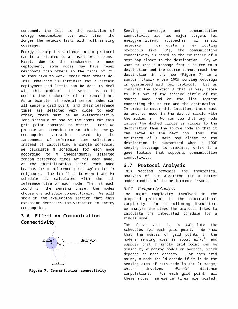
Figure 14. Actual Degree of Coverage for Differentiated Surveillance

6.7 Actual Degree of Coverage for Differentiated SurveillanceIn this simulation, we set the node density to be 5 per r2, and sample the actual degree of coverage for 100X100 grid points in the center. In addition to the proof from section 4, Figure 14 shows that our scheme can guarantee a degree of coverage to the desired value α for the target area. For example, if α is 2, then we guarantee that all grid points are covered by more than two sensor nodes and a single failure node will not affect the full coverage. However, the guaranteed α is the minimum possible degree of coverage for each grid point. Due to the protocol’s redundancy, most grid points are covered by a higher degree than the desired degree of coverage α. Figure 14 shows the distribution of actual degree of coverage for the grid points when we apply different desired degrees of coverage α. For example when α = 2, we guarantee that no grid point has an actual degree of coverage of less than 2. We acknowledge that the current solution only guarantees a sensor coverage lower bound and future work will continue to investigate the possibility to provide a sensor coverage upper bound for better energy conservation.

7. CONCLUSIONIn this paper, we introduce an adaptable sensing coverage mechanism for differentiated surveillance in sensor networks. Unlike previous schemes, our scheme guarantees not only full sensing coverage to a certain geographic area, but also the degree of coverage up to the limit imposed by the density of nodes available. The distinguishing advantages of our scheme are a much longer network half-life through energy conservation and balancing among sensor nodes, and a small communication overhead required to establish a working duty schedule among nodes. Several optimizations and extensions are proposed to provide even better performance. Simulations show that our protocol accomplishes differentiated surveillance with low energy consumption and outperforms other state-of-art schemes by as much as a 50% reduction in energy consumption and as much as a 130% increase in the half-life of the network.

8. ACKNOWLEDGEMENTSThis work was supported in part by NSF grant CCR-0098269, the MURI award N00014-01-1-0576 from ONR, and the DARPA IXO offices under the NEST project (grant number F336615-01-C-1905).

9. REFERENCES[1] G.H. Ahn, A. T. Campbell, A. Veres, and L. H. Sun,

“SWAN: Service Differentiation in Stateless Wireless Ad Hoc Networks,” IEEE INFOCOM'2002, New York, June 2002.

[2] S. Bhatnagar, B. Deb, and B. Nath, “Service Differentiation in Sensor Networks,” Fourth International Symposium on Wireless Personal Multimedia Communications, September 2001.

[3] S. Bhattacharya, H. Kim, S. Prabh, and T. Abdelzaher, “Energy-Conserving Data Placement and Asynchronous Multicast in Wireless Sensor Networks,” First International Conference on Mobile Systems, Applications, and Services (MobiSys), San Francisco, CA, May 2003.

[4] B. Chen , K. Jamieson, H. Balakrishnan, and R. Morris, “Span: An Energy-Efficient Coordination Algorithm for Topology Maintenance in Ad Hoc Wireless Networks,” Proceedings of the 6th ACM MOBICOM Conference, Rome, Italy, July 2001.

[5] Crossbow Technology, Inc., http://www.xbow.com/Products/Product_pdf_files/Wireless_pdf/6020-0042-01_A_MICA2.pdf.

[6] J. Elson, L. Girod, and D. Estrin, “Fine-Grained Network Time Synchronization using Reference Broadcasts,” Proceedings of the Fifth Symposium on Operating Systems Design and Implementation (OSDI 2002), Boston, MA.

[7] C. Guo, L. C. Zhong, and J. M. Rabaey, “Low Power Distributed MAC for Ad Hoc Sensor Radio Networks,” Proceedings of IEEE GlobeCom 2001, San Antonio, November 25-29, 2001.

[8] T. He, B. M. Blum, J. A. Stankovic, and T. F. Abdelzaher, “AIDA: Application Independent Data Aggregation in Wireless Sensor Networks,” ACM Transactions on Embedded Computing System, 2003, to appear.

[9] T. He, C. Huang, B. M. Blum, J. A. Stankovic, and T. F. Abdelzaher, “Range-Free Localization Schemes in Large Scale Sensor Networks,” MobiCom 2003, Sept. 2003.

[10] T. He, J. A. Stankovic, C. Lu, and T. F. Abdelzaher, “SPEED: A Stateless Protocol for Real-Time Communication in Sensor Networks,” International Conference on Distributed Computing Systems (ICDCS 2003), Providence, RI, May 2003.

[11] W. Heinzelman, A. Chandrakasan, and H. Balakrishnan, “Energy-Efficient Communication Protocol for Wireless Microsensor Networks,” HICSS '00, January 2000.

[12] C. Intanagonwiwat, D. Estrin, R. Govindan, and J. Heidemann, “Impact of Network Density on Data Aggregation in Wireless Sensor Networks,” Proceedings of the 22nd International Conference on Distributed Computing Systems, Vienna, Austria, IEEE. July 2002.

[13] B. Krishnamachari, D. Estrin, and S. Wicker, “Impact of

Data Aggregation in Wireless Sensor Networks,” International Workshop on Distributed Event-Based Systems, Vienna, Austria, July 2002.

[14] C. Lu, B. M. Blum, T. F. Abdelzaher, J. A. Stankovic, and T. He, “RAP: A Real-Time Communication Architecture for Large-Scale Wireless Sensor Networks,” IEEE RTAS 2002, San Jose, CA, September 2002.

[15] R. Min, M. Bhardwaj, S. H. Cho, A. Sinha, E. Shih, A. Wang, and A. Chandrakasan, “An Architecture for a Power-Aware Distributed Microsensor Node,” 2000 IEEE Workshop on Signal Processing Systems (SiPS '00), October 2000.

[16] R. Ramanathan and R. Rosales-Hain, “Topology control of multihop wireless networks using transmit power adjustment,” Proc. IEEE lnfocom 2000, March 2000.

[17] H. Takagi and L. Kleinrock, “Optimal Transmission Ranges For Randomly Distributed Packet Radio Terminals,” IEEE Trans. on Communications, 32(3):246-

257, March 1984.[18] D. Tian and N. D. Georganas, “A Node Scheduling

Scheme for Energy Conservation in Large Wireless Sensor Networks,” Wireless Communications and Mobile Computing Journal, May 2003.

[19] R. Williams, Geometrical Foundation of Natural Structure: A Source Book of Design, Dover Publications Inc, New York, pp. 51-52, 1979.

[20] Y. Xu, J. Heidemann, and D. Estrin, “Geography-informed Energy Conservation for Ad Hoc Routing,” ACM MOBICOM 2001, Rome, Italy, July 2001.

[21] Y. Xue and B. Li, “A Location-aided Power-aware Routing Protocol in Mobile Ad Hoc Networks,” Proceedings of IEEE Globecom 2001, Vol. 5, pp. 2837-2841, San Antonio, Texas, November 25-29, 2001.

[22] F. Ye, G. Zhong, S. Lu, and L. Zhang, “Energy Efficient Robust Sensing Coverage in Large Sensor Networks,” UCLA Technical Report 2002.