pathintegrals—elementarypropertiesand...
TRANSCRIPT
A dancing shape, an image gay,
To haunt, to startle, and waylay
W. Wordsworth (1770–1840), Phantom of Delight
2Path Integrals — Elementary Properties andSimple Solutions
The operator formalism of quantum mechanics and quantum statistics may notalways lead to the most transparent understanding of quantum phenomena. Thereexists another, equivalent formalism in which operators are avoided by the use ofinfinite products of integrals, called path integrals . In contrast to the Schrodingerequation, which is a differential equation determining the properties of a state at atime from their knowledge at an infinitesimally earlier time, path integrals yield thequantum-mechanical amplitudes in a global approach involving the properties of asystem at all times .
2.1 Path Integral Representation of Time Evolution
Amplitudes
The path integral approach to quantum mechanics was developed by Feynman1 in1942. In its original form, it applies to a point particle moving in a Cartesian co-ordinate system and yields the transition amplitudes of the time evolution operatorbetween the localized states of the particle (recall Section 1.7)
(xbtb|xata) = 〈xb|U(tb, ta)|xa〉, tb > ta. (2.1)
For simplicity, we shall at first assume the space to be one-dimensional. The exten-sion to D Cartesian dimensions will be given later. The introduction of curvilinearcoordinates will require a little more work. A further generalization to spaces witha nontrivial geometry, in which curvature and torsion are present, will be describedin Chapters 10–11.
2.1.1 Sliced Time Evolution Amplitude
We shall be interested mainly in the causal or retarded time evolution amplitudes[see Eq. (1.303)]. These contain all relevant quantum-mechanical information and
1For the historical development, see Notes and References at the end of this chapter.
89
90 2 Path Integrals — Elementary Properties and Simple Solutions
possess, in addition, pleasant analytic properties in the complex energy plane [seethe remarks after Eq. (1.310)]. This is why we shall always assume, from now on,the causal sequence of time arguments tb > ta.
Feynman realized that due to the fundamental composition law of the time evo-lution operator (see Section 1.7), the amplitude (2.1) could be sliced into a largenumber, say N + 1, of time evolution operators, each acting across an infinitesimaltime slice of thickness ǫ ≡ tn − tn−1= (tb − ta)/(N + 1)> 0:
(xbtb|xata) = 〈xb|U(tb, tN)U(tN , tN−1) · · · U(tn, tn−1) · · · U(t2, t1)U(t1, ta)|xa〉. (2.2)
When inserting a complete set of states between each pair of U ’s,
∫ ∞
−∞dxn|xn〉〈xn| = 1, n = 1, . . . , N, (2.3)
the amplitude becomes a product of N -integrals
(xbtb|xata) =N∏
n=1
[∫ ∞
−∞dxn
]N+1∏
n=1
(xntn|xn−1tn−1), (2.4)
where we have set xb ≡ xN+1, xa ≡ x0, tb ≡ tN+1, ta ≡ t0. The symbol Π[· · ·] denotesthe product of the quantities within the brackets. The integrand is the product ofthe amplitudes for the infinitesimal time intervals
(xntn|xn−1tn−1) = 〈xn|e−iǫH(tn)/h|xn−1〉, (2.5)
with the Hamiltonian operator
H(t) ≡ H(p, x, t). (2.6)
The further development becomes simplest under the assumption that the Hamil-tonian has the standard form, being the sum of a kinetic and a potential energy:
H(p, x, t) = T (p, t) + V (x, t). (2.7)
For a sufficiently small slice thickness, the time evolution operator
e−iǫH/h = e−iǫ(T+V )/h (2.8)
is factorizable as a consequence of the Baker-Campbell-Hausdorff formula (to beproved in Appendix 2A)
e−iǫ(T+V )/h = e−iǫV /he−iǫT /he−iǫ2X/h2
, (2.9)
where the operator X has the expansion
X ≡ i
2[V , T ]− ǫ
h
(
1
6[V , [V , T ]]− 1
3[[V , T ], T ]
)
+O(ǫ2) . (2.10)
2.1 Path Integral Representation of Time Evolution Amplitudes 91
The omitted terms of order ǫ4, ǫ5, . . . contain higher commutators of V and T . If weneglect, for the moment, the X-term which is suppressed by a factor ǫ2, we calculatefor the local matrix elements of e−iǫH/h the following simple expression:
〈xn|e−iǫH(p,x,tn)/h|xn−1〉 ≈∫ ∞
−∞dx〈xn|e−iǫV (x,tn)/h|x〉〈x|e−iǫT (p,tn)/h|xn−1〉
=∫ ∞
−∞dx〈xn|e−iǫV (x,tn)/h|x〉
∫ ∞
−∞
dpn2πh
eipn(x−xn−1)/he−iǫT (pn,tn)/h. (2.11)
Evaluating the local matrix elements,
〈xn|e−iǫV (x,tn)/h|x〉 = δ(xn − x)e−iǫV (xn,tn)/h, (2.12)
this becomes
〈xn|e−iǫH(p,x,tn)/h|xn−1〉 ≈∫ ∞
−∞
dpn2πh
exp ipn(xn − xn−1)/h− iǫ[T (pn, tn) + V (xn, tn)]/h . (2.13)
Inserting this back into (2.4), we obtain Feynman’s path integral formula, consistingof the multiple integral
(xbtb|xata) ≈N∏
n=1
[∫ ∞
−∞dxn
]N+1∏
n=1
[
∫ ∞
−∞
dpn2πh
]
exp(
i
hAN
)
, (2.14)
where AN is the sum
AN =N+1∑
n=1
[pn(xn − xn−1)− ǫH(pn, xn, tn)]. (2.15)
2.1.2 Zero-Hamiltonian Path Integral
Note that the path integral (2.14) with zero Hamiltonian produces the Hilbert spacestructure of the theory via a chain of scalar products:
(xbtb|xata) ≈N∏
n=1
[∫ ∞
−∞dxn
]N+1∏
n=1
[
∫ ∞
−∞
dpn2πh
]
ei∑N+1
n=1pn(xn−xn−1)/h, (2.16)
which is equal to
(xbtb|xata) ≈N∏
n=1
[∫ ∞
−∞dxn
] N+1∏
n=1
〈xn|xn−1〉 =N∏
n=1
[∫ ∞
−∞dxn
] N+1∏
n=1
δ(xn − xn−1)
= δ(xb − xa). (2.17)
whose continuum limit is
(xbtb|xata) =∫
Dx∫ Dp
2πhei∫
dtp(t)x(t)/h = 〈xb|xa〉 = δ(xb − xa). (2.18)
92 2 Path Integrals — Elementary Properties and Simple Solutions
In the operator expression (2.2), the right-hand side follows from the fact thatfor zero Hamiltonian the time evolution operators U(tn, tn−1) are all equal to unity.
At this point we make the important observation that a momentum variablepn inside the product of momentuma integrations in the expression (2.16) can begenerated by a derivative pn ≡ −ih∂xn outside of it. In Subsection 2.1.4 we shallgo to the continuum limit of time slicing in which the slice thickness ǫ goes to zero.In this limit, the discrete variables xn and pn become functions x(t) and p(t) of thecontinuous time t, and the momenta pn become differential operators p(t) = −ih∂x(t),satisfying the commutation relations with x(t):
[p(t), x(t)] = −ih. (2.19)
These are the canonical equal-time commutation relations of Heisenberg.This observation forms the basis for deriving, from the path integral (2.14), the
Schrodinger equation for the time evolution amplitude.
2.1.3 Schrodinger Equation for Time Evolution Amplitude
Let us split from the product of integrals in (2.14) the final time slice as a factor, sothat we obtain the recursion relation
(xbtb|xata) ≈∫ ∞
−∞dxN (xbtb|xN tN ) (xN tN |xata), (2.20)
where
(xbtb|xN tN ) ≈∫ ∞
−∞
dpb2πh
e(i/h)[pb(xb−xN )−ǫH(pb,xb,tb)]. (2.21)
The momentum pb inside the integral can be generated by a differential operatorpb ≡ −ih∂xb
outside of it. The same is true for any function of pb, so that theHamiltonian can be moved before the momentum integral yielding
(xbtb|xN tN)≈e−iǫH(−ih∂xb ,xb,tb)/h∫ ∞
−∞
dpb2πh
eipb(xb−xN )/h=e−iǫH(−ih∂xb ,xb,tb)/hδ(xb−xN ).(2.22)
Inserting this back into (2.20) we obtain
(xbtb|xata) ≈ e−iǫH(−ih∂xb ,xb,tb)/h(xb tb−ǫ|xata), (2.23)
or
1
ǫ[(xb tb+ǫ|xata)− (xbtb|xata)] ≈
1
ǫ
[
e−iǫH(−i∂xb ,xb,tb+ǫ)/h − 1]
(xb tb|xata). (2.24)
In the limit ǫ→ 0, this goes over into the differential equation for the time evolutionamplitude
ih∂tb(xbtb|xata) = H(−ih∂xb, xb, tb)(xb tb|xata), (2.25)
which is precisely the Schrodinger equation (1.301) of operator quantum mechanics.
2.1 Path Integral Representation of Time Evolution Amplitudes 93
2.1.4 Convergence of of the Time-Sliced Evolution Amplitude
Some remarks are necessary concerning the convergence of the time-sliced expression(2.14) to the quantum-mechanical amplitude in the continuum limit, where thethickness of the time slices ǫ = (tb − ta)/(N + 1) → 0 goes to zero and the numberN of slices tends to ∞. This convergence can be proved for the standard kineticenergy T = p2/2M only if the potential V (x, t) is sufficiently smooth. For time-independent potentials this is a consequence of the Trotter product formula whichreads
e−i(tb−ta)H/h = limN→∞
(
e−iǫV /he−iǫT /h)N+1
. (2.26)
If T and V are c-numbers, this is trivially true. If they are operators, we use Eq. (2.9)to rewrite the left-hand side of (2.26) as
e−i(tb−ta)H/h ≡(
e−iǫ(T+V )/h)N+1
≡(
e−iǫV /he−iǫT /he−iǫ2X/h2)N+1
.
The Trotter formula implies that the commutator term X proportional to ǫ2 doesnot contribute in the limit N → ∞. The mathematical conditions ensuring thisrequire functional analysis too technical to be presented here (for details, see theliterature quoted at the end of the chapter). For us it is sufficient to know thatthe Trotter formula holds for operators which are bounded from below and thatfor most physically interesting potentials, it cannot be used to derive Feynman’stime-sliced path integral representation (2.14), even in systems where the formulais known to be valid. In particular, the short-time amplitude may be differentfrom (2.13). Take, for example, an attractive Coulomb potential V (x) ∝ −1/|x|for which the Trotter formula has been proved to be valid. Feynman’s time-slicedformula, however, diverges even for two time slices. This will be discussed in detail inChapter 12. Similar problems will be found for other physically relevant potentialssuch as V (x) ∝ l(l +D − 2)h2/|x|2 (centrifugal barrier) and V (θ) ∝ m2h2/sin2 θ(angular barrier near the poles of a sphere). In all these cases, the commutatorsin the expansion (2.10) of X become more and more singular. In fact, as we shallsee, the expansion does not even converge, even for an infinitesimally small ǫ. Allatomic systems contain such potentials and the Feynman formula (2.14) cannot beused to calculate an approximation for the transition amplitude. A new path integralformula has to be found. This will be done in Chapter 12. Fortunately, it is possibleto eventually reduce the more general formula via some transformations back to aFeynman type formula with a bounded potential in an auxiliary space. Thus theabove derivation of Feynman’s formula for such potentials will be sufficient for thefurther development in this book. After this it serves as an independent startingpoint for all further quantum-mechanical calculations.
In the sequel, the symbol ≈ in all time-sliced formulas such as (2.14) will implythat an equality emerges in the continuum limit N → ∞, ǫ→ 0 unless the potential
94 2 Path Integrals — Elementary Properties and Simple Solutions
has singularities of the above type. In the action, the continuum limit is withoutsubtleties. The sum AN in (2.15) tends towards the integral
A[p, x] =∫ tb
tadt [p(t)x(t)−H(p(t), x(t), t)] (2.27)
under quite general circumstances. This expression is recognized as the classicalcanonical action for the path x(t), p(t) in phase space. Since the position variablesxN+1 and x0 are fixed at their initial and final values xb and xa, the paths satisfythe boundary condition x(tb) = xb, x(ta) = xa.
In the same limit, the product of infinitely many integrals in (2.14) will be calleda path integral . The limiting measure of integration is written as
limN→∞
N∏
n=1
[∫ ∞
−∞dxn
]N+1∏
n=1
[
∫ ∞
−∞
dpn2πh
]
≡∫ x(tb)=xb
x(ta)=xa
D′x∫ Dp
2πh. (2.28)
By definition, there is always one more pn-integral than xn-integrals in this product.While x0 and xN+1 are held fixed and the xn-integrals are done for n = 1, . . . , N , eachpair (xn, xn−1) is accompanied by one pn-integral for n = 1, . . . , N+1. The situationis recorded by the prime on the functional integral D′x. With this definition, theamplitude can be written in the short form
(xbtb|xata) =∫ x(tb)=xb
x(ta)=xa
D′x∫ Dp
2πheiA[p,x]/h. (2.29)
The path integral has a simple intuitive interpretation: Integrating over all pathscorresponds to summing over all histories along which a physical system can possiblyevolve. The exponential eiA[p,x]/h is the quantum analog of the Boltzmann factore−E/kBT in statistical mechanics. Instead of an exponential probability, a pure phasefactor is assigned to each possible history: The total amplitude for going from xa, tato xb, tb is obtained by adding up the phase factors for all these histories,
(xbtb|xata) =∑
all histories(xa,ta) (xb,tb)
eiA[p,x]/h, (2.30)
where the sum comprises all paths in phase space with fixed endpoints xb, xa inx-space.
2.1.5 Time Evolution Amplitude in Momentum Space
The above observed asymmetry in the functional integrals over x and p is a conse-quence of keeping the endpoints fixed in position space. There exists the possibilityof proceeding in a conjugate way keeping the initial and final momenta pb and pafixed. The associated time evolution amplitude can be derived by going throughthe same steps as before but working in the momentum space representation of theHilbert space, starting from the matrix elements of the time evolution operator
(pbtb|pata) ≡ 〈pb|U(tb, ta)|pa〉. (2.31)
2.1 Path Integral Representation of Time Evolution Amplitudes 95
The time slicing proceeds as in (2.2)–(2.4), with all x’s replaced by p’s, except inthe completeness relation (2.3) which we shall take as
∫ ∞
−∞
dp
2πh|p〉〈p| = 1, (2.32)
corresponding to the choice of the normalization of states [compare (1.186)]
〈pb|pa〉 = 2πhδ(pb − pa). (2.33)
In the resulting product of integrals, the integration measure has an opposite asym-metry: there is now one more xn-integral than pn-integrals. The sliced path integralreads
(pbtb|pata) ≈N∏
n=1
[
∫ ∞
−∞
dpn2πh
]
N∏
n=0
[∫ ∞
−∞dxn
]
× exp
i
h
N∑
n=0
[−xn(pn+1 − pn)− ǫH(pn, xn, tn)]
. (2.34)
The relation between this and the x-space amplitude (2.14) is simple: By takingin (2.14) the first and last integrals over p1 and pN+1 out of the product, renamingthem as pa and pb, and rearranging the sum
∑N+1n=1 pn(xn − xn−1) as follows
N+1∑
n=1
pn(xn − xn−1) = pN+1(xN+1 − xN ) + pN(xN − xN−1) + . . .
. . .+ p2(x2 − x1) + p1(x1 − x0)
= pN+1xN+1 − p1x0
−(pN+1 − pN)xN − (pN − pN−1)xN−1 − . . .− (p2 − p1)x1
= pN+1xN+1 − p1x0 −N∑
n=1
(pn+1 − pn)xn, (2.35)
the remaining product of integrals looks as in Eq. (2.34), except that the lowestindex n is one unit larger than in the sum in Eq. (2.34). In the limit N → ∞ thisdoes not matter, and we obtain the Fourier transform
(xbtb|xata) =∫ dpb
2πheipbxb/h
∫ dpa2πh
e−ipaxa/h(pbtb|pata). (2.36)
The inverse relation is
(pbtb|pata) =∫
dxb e−ipbxb/h
∫
dxa eipaxa/h(xbtb|xata). (2.37)
In the continuum limit, the amplitude (2.34) can be written as a path integral
(pbtb|pata) =∫ p(tb)=pb
p(ta)=pa
D′p
2πh
∫
DxeiA[p,x]/h, (2.38)
96 2 Path Integrals — Elementary Properties and Simple Solutions
where
A[p, x] =∫ tb
tadt [−p(t)x(t)−H(p(t), x(t), t)] = A[p, x]− pbxb + paxa. (2.39)
If the Hamiltonian is independent of x and t, the sliced path integral (2.34)becomes trivial. Then the N + 1 integrals over xn (n = 0, . . . , N) can be doneyielding a product of δ-functions δ(pb − pN) · · · δ(p1 − p0). As a conseqence, theintegrals over the N momenta pn (n = 1, . . . , N) are all squeezed to the initialmomentum pN = pN−1 = . . . = p1 = pa. A single a final δ-function 2πhδ(pb − pa)remains, accompanied by the product of N + 1 factors
∏Nn=0 e
−iǫH(pa)/h, which isequal to e−i(tb−ta)H(p)/h. Hence we obtain:
(pbtb|pata) = 2πhδ(pb − pa)e−i(tb−ta)H(p)/h. (2.40)
Inserting this into Eq. (2.36), we find a simple Fourier integral for the time evolutionamlitude in x-space:
(xbtb|xata) =∫
dp
2πheip(xb−xa)/h−i(tb−ta)H(p)/h. (2.41)
Note that in (2.40) contains an equal sign rather than the ≈-sign since the right-handsign is the same for any number of time slices.
2.1.6 Quantum-Mechanical Partition Function
A path integral symmetric in p and x arises when considering the quantum-mechanical partition function defined by the trace (recall Section 1.17)
ZQM(tb, ta) = Tr(
e−i(tb−ta)H/h)
. (2.42)
In the local basis, the trace becomes an integral over the amplitude(xbtb|xata) with xb = xa:
ZQM(tb, ta) =∫ ∞
−∞dxa(xatb|xata). (2.43)
The additional trace integral over xN+1 ≡ x0 makes the path integral for ZQM
symmetric in pn and xn:
∫ ∞
−∞dxN+1
N∏
n=1
[∫ ∞
−∞dxn
]N+1∏
n=1
[
∫ ∞
−∞
dpn2πh
]
=N+1∏
n=1
[
∫∫ ∞
−∞
dxndpn2πh
]
. (2.44)
In the continuum limit, the right-hand side is written as
limN→∞
N+1∏
n=1
[
∫∫ ∞
−∞
dxndpn2πh
]
≡∮
Dx∫ Dp
2πh, (2.45)
2.1 Path Integral Representation of Time Evolution Amplitudes 97
and the measures are related by
∫ ∞
−∞dxa
∫ x(tb)=xa
x(ta)=xa
D′x∫ Dp
2πh≡∮
Dx∫ Dp
2πh. (2.46)
The symbol∮
indicates the periodic boundary condition x(ta) = x(tb). In themomentum representation we would have similarly
∫ ∞
−∞
dpa2πh
∫ p(tb)=pa
p(ta)=pa
D′p
2πh
∫
Dx ≡∮ Dp
2πh
∫
Dx , (2.47)
with the periodic boundary condition p(ta) = p(tb), and the same right-hand side.Hence, the quantum-mechanical partition function is given by the path integral
ZQM(tb, ta) =∮
Dx∫ Dp
2πheiA[p,x]/h =
∮ Dp2πh
∫
DxeiA[p,x]/h. (2.48)
In the right-hand exponential, the action A[p, x] can be replaced by A[p, x], sincethe extra terms in (2.39) are removed by the periodic boundary conditions. In thetime-sliced expression, the equality is easily derived from the rearrangement of thesum (2.35), which shows that
N+1∑
n=1
pn(xn − xn−1)
∣
∣
∣
∣
∣
xN+1=x0
= −N∑
n=0
(pn+1 − pn)xn
∣
∣
∣
∣
∣
pN+1=p0
. (2.49)
In the path integral expression (2.48) for the partition function, the rules of quan-tum mechanics appear as a natural generalization of the rules of classical statisticalmechanics, as formulated by Planck. According to these rules, each volume elementin phase space dxdp/h is occupied with the exponential probability e−E/kBT . In thepath integral formulation of quantum mechanics, each volume element in the path
phase space∏
n dx(tn)dp(tn)/h is associated with a pure phase factor eiA[p,x]/h. Wesee here a manifestation of the correspondence principle which specifies the tran-sition from classical to quantum mechanics. In path integrals, it looks somewhatmore natural than in the historic formulation, where it requires the replacement ofall classical phase space variables p, x by operators, a rule which was initially hardto comprehend.
2.1.7 Feynman’s Configuration Space Path Integral
Actually, in his original paper, Feynman did not give the path integral formula inthe above phase space formulation. Since the kinetic energy in (2.7) has usually theform T (p, t) = p2/2M , he focused his attention upon the Hamiltonian
H =p2
2M+ V (x, t), (2.50)
98 2 Path Integrals — Elementary Properties and Simple Solutions
for which the time-sliced action (2.15) becomes
AN =N+1∑
n=1
[
pn(xn − xn−1)− ǫp2n2M
− ǫV (xn, tn)
]
. (2.51)
It can be quadratically completed to
AN =N+1∑
n=1
[
− ǫ
2M
(
pn −xn − xn−1
ǫM)2
+M
2ǫ(
xn − xn−1
ǫ
)2
− ǫV (xn, tn)
]
. (2.52)
The momentum integrals in (2.14) may then be performed using the Fresnel integralformula (1.337), yielding
∫ ∞
−∞
dpn2πh
exp
[
− i
h
ǫ
2M
(
pn −Mxn − xn−1
ǫ
)2]
=1
√
2πhiǫ/M, (2.53)
and we arrive at the alternative representation
(xbtb|xata) ≈1
√
2πhiǫ/M
N∏
n=1
∫ ∞
−∞
dxn√
2πhiǫ/M
exp(
i
hAN
)
, (2.54)
where AN is now the sum
AN = ǫN+1∑
n=1
[
M
2
(
xn − xn−1
ǫ
)2
− V (xn, tn)
]
, (2.55)
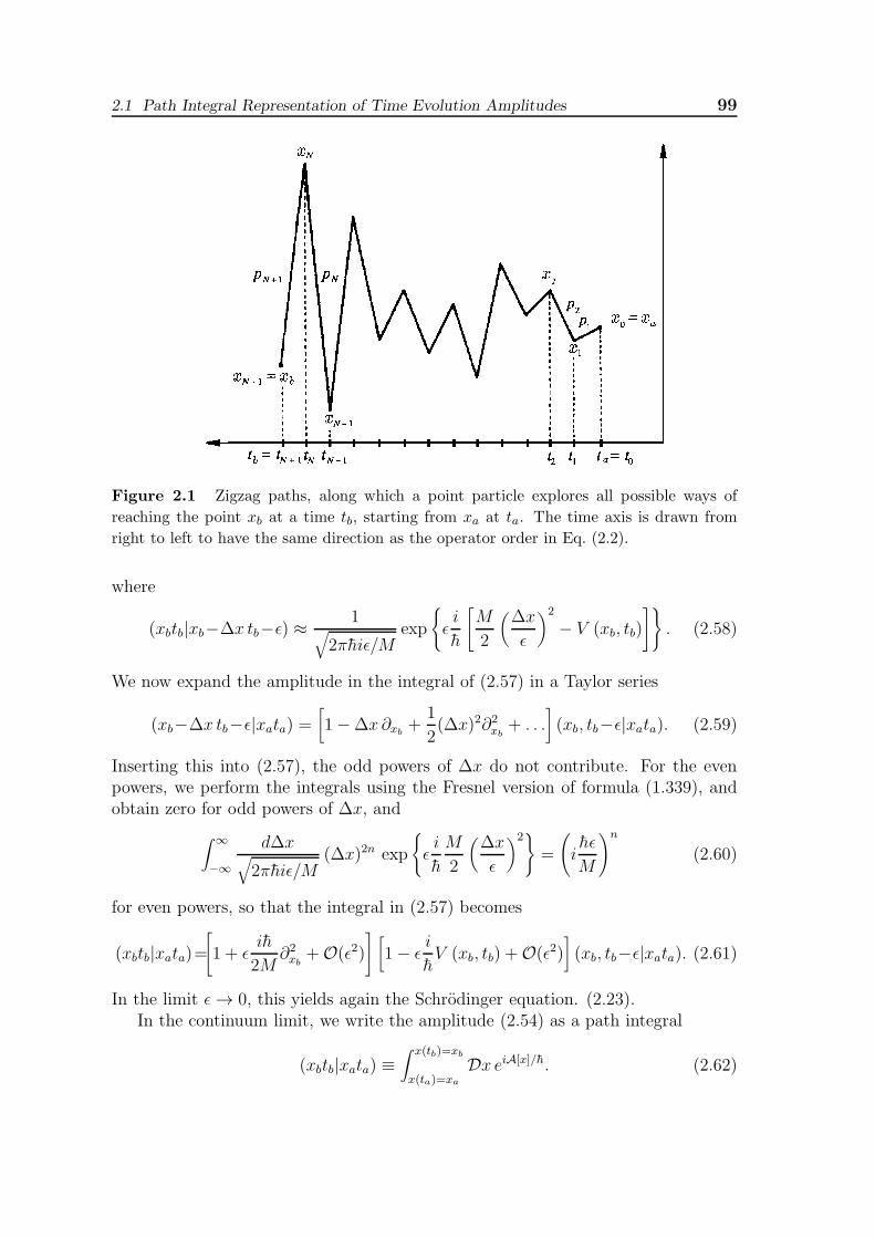
with xN+1 = xb and x0 = xa. Here the integrals run over all paths in configuration
space rather than phase space. They account for the fact that a quantum-mechanicalparticle starting from a given initial point xa will explore all possible ways of reachinga given final point xb. The amplitude of each path is exp(iAN/h). See Fig. 2.1 fora geometric illustration of the path integration. In the continuum limit, the sum(2.55) converges towards the action in the Lagrangian form:
A[x] =∫ tb
tadtL(x, x) =
∫ tb
tadt[
M
2x2 − V (x, t)
]
. (2.56)
Note that this action is a local functional of x(t) in the temporal sense as defined inEq. (1.26).2
For the time-sliced Feynman path integral, one verifies the Schrodinger equationas follows: As in (2.20), one splits off the last slice as follows:
(xbtb|xata) ≈∫ ∞
−∞dxN (xbtb|xN tN ) (xN tN |xata)
=∫ ∞
−∞d∆x (xbtb|xb−∆x tb−ǫ) (xb−∆x tb−ǫ|xata), (2.57)
2A functional F [x] is called local if it can be written as an integral∫
dtf(x(t), x(t)); it is calledultra-local if it has the form
∫
dtf(x(t)).
2.1 Path Integral Representation of Time Evolution Amplitudes 99
Figure 2.1 Zigzag paths, along which a point particle explores all possible ways of
reaching the point xb at a time tb, starting from xa at ta. The time axis is drawn from
right to left to have the same direction as the operator order in Eq. (2.2).
where
(xbtb|xb−∆x tb−ǫ) ≈1
√
2πhiǫ/Mexp
ǫi
h
[
M
2
(
∆x
ǫ
)2
− V (xb, tb)
]
. (2.58)
We now expand the amplitude in the integral of (2.57) in a Taylor series
(xb−∆x tb−ǫ|xata) =[
1−∆x ∂xb+
1
2(∆x)2∂2xb
+ . . .]
(xb, tb−ǫ|xata). (2.59)
Inserting this into (2.57), the odd powers of ∆x do not contribute. For the evenpowers, we perform the integrals using the Fresnel version of formula (1.339), andobtain zero for odd powers of ∆x, and
∫ ∞
−∞
d∆x√
2πhiǫ/M(∆x)2n exp
ǫi
h
M
2
(
∆x
ǫ
)2
=
(
ihǫ
M
)n
(2.60)
for even powers, so that the integral in (2.57) becomes
(xbtb|xata)=[
1 + ǫih
2M∂2xb
+O(ǫ2)
]
[
1− ǫi
hV (xb, tb) +O(ǫ2)
]
(xb, tb−ǫ|xata). (2.61)
In the limit ǫ→ 0, this yields again the Schrodinger equation. (2.23).In the continuum limit, we write the amplitude (2.54) as a path integral
(xbtb|xata) ≡∫ x(tb)=xb
x(ta)=xa
Dx eiA[x]/h. (2.62)
100 2 Path Integrals — Elementary Properties and Simple Solutions
This is Feynman’s original formula for the quantum-mechanical amplitude (2.1). Itconsists of a sum over all paths in configuration space with a phase factor containingthe form of the action A[x].
We have used the same measure symbol Dx for the paths in configuration spaceas for the completely different paths in phase space in the expressions (2.29), (2.38),(2.46), (2.47). There should be no danger of confusion. Note that the extra dpn-
integration in the phase space formula (2.14) results now in one extra 1/√
2πhiǫ/M
factor in (2.54) which is not accompanied by a dxn-integration.The Feynman amplitude can be used to calculate the quantum-mechanical par-
tition function (2.43) as a configuration space path integral
ZQM =∮
Dx eiA[x]/h. (2.63)
As in (2.45), (2.46), the symbol∮ Dx indicates that the paths have equal endpoints
x(ta) = x(tb), the path integral being the continuum limit of the product of integrals
∮
Dx ≈N+1∏
n=1
∫ ∞
−∞
dxn√
2πihǫ/M. (2.64)
There is no extra 1/√
2πihǫ/M factor as in (2.54) and (2.62), due to the integration
over the initial (= final) position xb = xa representing the quantum-mechanicaltrace. The use of the same symbol
∮ Dx as in (2.48) should not cause any confusionsince (2.48) is always accompanied by an integral
∫ Dp.For the sake of generality we might point out that it is not necessary to slice the
time axis in an equidistant way. In the continuum limit N → ∞, the canonical pathintegral (2.14) is indifferent to the choice of the infinitesimal spacings
ǫn = tn − tn−1. (2.65)
The configuration space formula contains the different spacings ǫn in the followingway: When performing the pn integrations, we obtain a formula of the type (2.54),with each ǫ replaced by ǫn, i.e.,
(xbtb|xata) ≈1
√
2πhiǫb/M
N∏
n=1
∫ ∞
−∞
dxn√
2πihǫn/M
× exp
i
h
N+1∑
n=1
[
M
2
(xn − xn−1)2
ǫn− ǫnV (xn, tn)
]
. (2.66)
To end this section, an important remark is necessary: It would certainly bepossible to define the path integral for the time evolution amplitude (2.29), withoutgoing through Feynman’s time-slicing procedure, as the solution of the Schrodingerdifferential equation [see Eq. (1.308))]:
[H(−ih∂x, x)− ih∂t](x t|xata) = −ihδ(t− ta)δ(x− xa). (2.67)
2.2 Exact Solution for the Free Particle 101
If one possesses an orthonormal and complete set of wave functions ψn(x) solvingthe time-independent Schrodinger equation Hψn(x)=Enψn(x), this solution is givenby the spectral representation (1.323)
(xbtb|xata) = Θ(tb − ta)∑
n
ψn(xb)ψ∗n(xa)e
−iEn(tb−ta)/h, (2.68)
where Θ(t) is the Heaviside function (1.304). This definition would, however, runcontrary to the very purpose of Feynman’s path integral approach, which is to un-derstand a quantum system from the global all-time fluctuation point of view. Thegoal is to find all properties from the globally defined time evolution amplitude, inparticular the Schrodinger wave functions.3 The global approach is usually morecomplicated than Schrodinger’s and, as we shall see in Chapters 8 and 12–14, con-tains novel subtleties caused by the finite time slicing. Nevertheless, it has at leastfour important advantages. First, it is conceptually very attractive by formulatinga quantum theory without operators which describe quantum fluctuations by closeanalogy with thermal fluctuations (as will be seen later in this chapter). Second,it links quantum mechanics smoothly with classical mechanics (as will be shown inChapter 4). Third, it offers new variational procedures for the approximate study ofcomplicated quantum-mechanical and -statistical systems (see Chapter 5). Fourth,it gives a natural geometric access to the dynamics of particles in spaces with cur-vature and torsion (see Chapters 10–11). This has recently led to results wherethe operator approach has failed due to operator-ordering problems, giving rise toa unique and correct description of the quantum dynamics of a particle in spaceswith curvature and torsion. From this it is possible to derive a unique extensionof Schrodinger’s theory to such general spaces whose predictions can be tested infuture experiments.4
2.2 Exact Solution for the Free Particle
In order to develop some experience with Feynman’s path integral formula we con-sider in detail the simplest case of a free particle, which in the canonical form reads
(xbtb|xata) =∫ x(tb)=xb
x(ta)=xa
D′x∫ Dp
2πhexp
[
i
h
∫ tb
tadt
(
px− p2
2M
)]
, (2.69)
and in the pure configuration form:
(xbtb|xata) =∫ x(tb)=xb
x(ta)=xa
Dx exp[
i
h
∫ tb
tadtM
2x2]
. (2.70)
Since the integration limits are obvious by looking at the left-hand sides of the equa-tions, they will be omitted from now on, unless clarity requires their specification.
3Many publications claiming to have solved the path integral of a system have violated this ruleby implicitly using the Schrodinger equation, although camouflaged by complicated-looking pathintegral notation.
4H. Kleinert, Mod. Phys. Lett. A 4 , 2329 (1989) (http://www.physik.fu-berlin.de/~klei-nert/199); Phys. Lett. B 236 , 315 (1990) (ibid.http/202).
102 2 Path Integrals — Elementary Properties and Simple Solutions
2.2.1 Trivial Solution
Since the Hamiltonian of a free particle H = p2/2M does not depend on x, the pathintegral in momentum space yields the simple result (2.40). In configuration spaceit reduces to simple Fourier integral Eq. (2.41). Inserting the above Hamiltonian,the integral reads
(xbtb|xata) =∫
dp
2πheip(xb−xa)/h−i(tb−ta)p2/2Mh, (2.71)
and can be done with the help of the Fresnel formula (2.53). The result is
(xbtb|xata) =1
√
2πih(tb − ta)/Mexp
[
i
h
M
2
(xb − xa)2
tb − ta
]
. (2.72)
This result is easily generalized to D dimensions, where the free-particle ampli-tude (2.40) reads
(pbtb|pata) = (2πh)Dδ(D)(pb − pa)e−i(tb−ta)p2/2Mh, (2.73)
and the Fourier transform yields
(xbtb|xata) =1
√
2πih(tb − ta)/MD exp
[
i
h
M
2
(xb − xa)2
tb − ta
]
, (2.74)
in agreement with the quantum-mechanical result in D dimensions (1.341).
2.2.2 Solution in Configuration Space
The problem can also be solved with little effort starting from Eq. (2.70). The time-sliced expression to be integrated is given by Eqs. (2.54), (2.55) with V (x) set equalto zero. The resulting product of Gaussian integrals can easily be done successivelyusing formula (1.337), from which we derive the simple rule
∫
dx′1
√
2πihAǫ/Mexp
[
i
h
M
2
(x′′ − x′)2
Aǫ
]
1√
2πihBǫ/Mexp
[
i
h
M
2
(x′ − x)2
Bǫ
]
=1
√
2πih(A +B)ǫ/Mexp
[
i
h
M
2
(x′′ − x)2
(A+B)ǫ
]
, (2.75)
which leads directly to the free-particle amplitude
(xbtb|xata) =1
√
2πih(N + 1)ǫ/Mexp
[
i
h
M
2
(xb − xa)2
(N + 1)ǫ
]
. (2.76)
After inserting (N + 1)ǫ = tb − ta, this agrees with the previous result (2.72). Notethat the free-particle amplitude happens to be independent of the number N + 1 oftime slices.
2.2 Exact Solution for the Free Particle 103
The calculation shows that the path integrals (2.69) and (2.70) possess a simplesolvable generalization to a time-dependent mass M(t) =Mg(t):
(xbtb|xata) =∫ x(tb)=xb
x(ta)=xa
D′x∫ Dp
2πhexp
[
i
h
∫ tb
tadt
(
px− p2
2Mg(t)
)]
, (2.77)
and in the pure configuration form:
(xbtb|xata) =∫ x(tb)=xb
x(ta)=xa
Dx√g exp[
i
h
∫ tb
tadtM
2g(t)x2(t)
]
. (2.78)
Here the measure of integration∫ Dx√g symbolizes the continuum limit of the
product [compare (2.54)]:
∫ x(tb)=xb
x(ta)=xa
Dx√g ≡ 1√
2πhiǫ/Mg(tb)
N∏
n=1
∫ ∞
−∞
dxn√
2πhiǫ/Mg(tn)
. (2.79)
The factor g(tn) enters in each of the integrations (2.75), where the previous timeslicing parameters ǫ becomes now ǫn = ǫ/g(tn), and we find instead of (2.72) theamplitude
(xbtb|xata) =1
√
2πihM−1∫ tbtag−1(t)
exp
[
i
h
M
2
(xb − xa)2
∫ tbta g
−1(t)
]
. (2.80)
This has the Fourier representation
(xbtb|xata) =∫
dp
2πhexp
i
h
[
ip(xb − xa)−p2
2M
∫ tb
tag−1(t)
]
. (2.81)
2.2.3 Fluctuations around the Classical Path
There exists yet another method of calculating this amplitude which is somewhatinvolved than the simple case at hand deserves, but which turns out to be useful forthe treatment of a certain class of more complicated path integrals, after a suitablegeneralization. This method is based on summing aver all path deviations from theclassical path, i.e., all paths are split into the classical path
xcl(t) = xa +xb − xatb − ta
(t− ta), (2.82)
along which the free particle would run following the equation of motion
xcl(t) = 0, (2.83)
plus deviations δx(t):
x(t) = xcl(t) + δx(t). (2.84)
104 2 Path Integrals — Elementary Properties and Simple Solutions
Since the initial and final points are fixed at xa, xb, respectively, the deviations vanishat the endpoints:
δx(ta) = δx(tb) = 0. (2.85)
The deviations δx(t) are referred to as the quantum fluctuations of the particleorbit. In mathematics, the boundary conditions (2.85) are referred to as Dirichlet
boundary conditions . When inserting the decomposition (2.84) into the action weobserve that due to the equation of motion (2.83) for the classical path, the actionseparates into the sum of a classical and a purely quadratic fluctuation term
M
2
∫ tb
tadt
x2cl(t) + 2xcl(t)δx(t) + [δx(t)]2
=M
2
∫ tb
tadtx2cl +Mxδx
∣
∣
∣
tb
ta−M
∫ tb
tadtxclδx+
M
2
∫ tb
tadt(δx)2
=M
2
[∫ tb
tadtx2cl +
∫ tb
tadt(δx)2
]
.
The absence of a mixed term is a general consequence of the extremality propertyof the classical path,
δA∣
∣
∣
x(t)=xcl(t)= 0. (2.86)
It implies that a quadratic fluctuation expansion around the classical action
Acl ≡ A[xcl] (2.87)
can have no linear term in δx(t), i.e., it must start as
A = Acl +1
2
∫ tb
tadt∫ tb
tadt′
δ2Aδx(t)δx(t′)
δx(t)δx(t′)
∣
∣
∣
∣
x(t)=xcl(t)+ . . . . (2.88)
With the action being a sum of two terms, the amplitude factorizes into the productof a classical amplitude eiAcl/h and a fluctuation factor F0(tb − ta),
(xbtb|xata) =∫
Dx eiA[x]/h = eiAcl/hF0(tb, ta). (2.89)
For the free particle with the classical action
Acl =∫ tb
tadtM
2x2cl, (2.90)
the function factor F0(tb − ta) is given by the path integral
F0(tb − ta) =∫
Dδx(t) exp[
i
h
∫ tb
tadtM
2(δx)2
]
. (2.91)
Due to the vanishing of δx(t) at the endpoints, this does not depend on xb, xa butonly on the initial and final times tb, ta. The time translational invariance reduces
2.2 Exact Solution for the Free Particle 105
this dependence further to the time difference tb−ta. The subscript zero of F0(tb−ta)indicates the free-particle nature of the fluctuation factor. After inserting (2.82) into(2.90), we find immediately
Acl =M
2
(xb − xa)2
tb − ta. (2.92)
The fluctuation factor, on the other hand, requires the evaluation of the multipleintegral
FN0 (tb − ta) =
1√
2πhiǫ/M
N∏
n=1
∫ ∞
−∞
dδxn√
2πhiǫ/M
exp(
i
hAN
fl
)
, (2.93)
where ANfl is the time-sliced fluctuation action
ANfl =
M
2ǫN+1∑
n=1
(
δxn − δxn−1
ǫ
)2
. (2.94)
At the end, we have to take the continuum limit
N → ∞, ǫ = (tb − ta)/(N + 1) → 0.
2.2.4 Fluctuation Factor
The remainder of this section will be devoted to calculating the fluctuation factor(2.93). Before doing this, we shall develop a general technique for dealing withsuch time-sliced expressions. Due to the frequent appearance of the fluctuatingδx-variables, we shorten the notation by omitting all δ’s and working only withx-variables.
A useful device for manipulating sums on a sliced time axis such as (2.94) is thedifference operator ∇ and its conjugate ∇, defined by
∇x(t) ≡ 1
ǫ[x(t + ǫ)− x(t)], ∇x(t) ≡ 1
ǫ[x(t)− x(t− ǫ)]. (2.95)
They are two different discrete versions of the time derivative ∂t, to which bothreduce in the continuum limit ǫ→ 0:
∇,∇ ǫ→0−−−→ ∂t, (2.96)
if they act upon differentiable functions. Since the discretized time axis with N +1steps constitutes a one-dimensional lattice, the difference operators ∇,∇ are alsocalled lattice derivatives .
For the coordinates xn = x(tn) at the discrete times tn we write
∇xn =1
ǫ(xn+1 − xn), N ≥ n ≥ 0,
∇xn =1
ǫ(xn − xn−1), N + 1 ≥ n ≥ 1. (2.97)
106 2 Path Integrals — Elementary Properties and Simple Solutions
The time-sliced action (2.94) can then be expressed in terms of ∇xn or ∇xn as(writing xn instead of δxn)
ANfl =
M
2ǫ
N∑
n=0
(∇xn)2 =M
2ǫN+1∑
n=1
(∇xn)2. (2.98)
In this notation, the limit ǫ → 0 is most obvious: The sum ǫ∑
n goes into theintegral
∫ tbta dt, whereas both (∇xn)2 and (∇xn)2 tend to x2, so that
ANfl →
∫ tb
tadtM
2x2. (2.99)
Thus, the time-sliced action becomes the Lagrangian action.Lattice derivatives have properties quite similar to ordinary derivatives. One
only has to be careful in distinguishing ∇ and ∇. For example, they allow for theuseful operation summation by parts which is analogous to integration by parts.Recall the rule for the integration by parts
∫ tb
tadtg(t)f(t) = g(t)f(t)
∣
∣
∣
tb
ta−∫ tb
tadtg(t)f(t). (2.100)
On the lattice, this relation yields for functions f(t) → xn and g(t) → pn:
ǫN+1∑
n=1
pn∇xn = pnxn|N+10 − ǫ
N∑
n=0
(∇pn)xn. (2.101)
This follows directly by rewriting (2.35).For functions vanishing at the endpoints, i.e., for xN+1 = x0 = 0, we can omit
the surface terms and shift the range of the sum on the right-hand side to obtainthe simple formula [see also Eq. (2.49)]
N+1∑
n=1
pn∇xn = −N∑
n=0
(∇pn)xn = −N+1∑
n=1
(∇pn)xn. (2.102)
The same thing holds if both p(t) and x(t) are periodic in the interval tb− ta, so thatp0 = pN+1, x0 = xN+1. In this case, it is possible to shift the sum on the right-handside by one unit arriving at the more symmetric-looking formula
N+1∑
n=1
pn∇xn = −N+1∑
n=1
(∇pn)xn. (2.103)
In the time-sliced action (2.94) the quantum fluctuations xn (=δxn) vanish at theends, so that (2.102) can be used to rewrite
N+1∑
n=1
(∇xn)2 = −N∑
n=1
xn∇∇xn. (2.104)
2.2 Exact Solution for the Free Particle 107
In the ∇xn -form of the action (2.98), the same expression is obtained by applyingformula (2.102) from the right- to the left-hand side and using the vanishing of x0and xN+1:
N∑
n=0
(∇xn)2 = −N+1∑
n=1
xn∇∇xn = −N∑
n=1
xn∇∇xn. (2.105)
The right-hand sides in (2.104) and (2.105) can be written in matrix form as
−N∑
n=1
xn∇∇xn ≡ −N∑
n,n′=1
xn(∇∇)nn′xn′ ,
−N∑
n=1
xn∇∇xn ≡ −N∑
n,n′=1
xn(∇∇)nn′xn′ , (2.106)
with the same N ×N -matrix
∇∇ ≡ ∇∇ ≡ 1
ǫ2
−2 1 0 . . . 0 0 01 −2 1 . . . 0 0 0...
...0 0 0 . . . 1 −2 10 0 0 . . . 0 1 −2
. (2.107)
This is obviously the lattice version of the double time derivative ∂2t , to which itreduces in the continuum limit ǫ→ 0. It will therefore be called the lattice Laplacian.
A further common property of lattice and ordinary derivatives is that they canboth be diagonalized by going to Fourier components. When decomposing
x(t) =∫ ∞
−∞dωe−iωtx(ω), (2.108)
and applying the lattice derivative ∇, we find
∇x(tn) =∫ ∞
−∞dω
1
ǫ
(
e−iω(tn+ǫ) − e−iωtn)
x(ω) (2.109)
=∫ ∞
−∞dωe−iωtn
1
ǫ(e−iωǫ − 1) x(ω).
Hence, on the Fourier components, ∇ has the eigenvalues
1
ǫ(e−iωǫ − 1). (2.110)
In the continuum limit ǫ → 0, this becomes the eigenvalue of the ordinary timederivative ∂t, i.e., −i times the frequency of the Fourier component ω. As a reminderof this we shall denote the eigenvalue of i∇ by Ω and have
(i∇x)(ω) = Ω x(ω) ≡ i
ǫ(e−iωǫ − 1) x(ω). (2.111)
108 2 Path Integrals — Elementary Properties and Simple Solutions
For the conjugate lattice derivative we find similarly
(i∇x)(ω) = Ω x(ω) ≡ − iǫ(eiωǫ − 1) x(ω), (2.112)
where Ω is the complex-conjugate number of Ω, i.e., Ω ≡ Ω∗. As a consequence, theeigenvalues of the negative lattice Laplacian −∇∇≡−∇∇ are real and nonnegative:
i
ǫ(e−iωǫ − 1)
i
ǫ(1− eiωǫ) =
1
ǫ2[2− 2 cos(ωǫ)] ≥ 0. (2.113)
Of course, Ω and Ω have the same continuum limit ω.When decomposing the quantum fluctuations x(t) [=δx(t)] into their Fourier
components, not all eigenfunctions occur. Since x(t) vanishes at the initial timet = ta, the decomposition can be restricted to the sine functions and we may expand
x(t) =∫ ∞
0dω sinω(t− ta) x(ω). (2.114)
The vanishing at the final time t = tb is enforced by a restriction of the frequenciesω to the discrete values
νm =πm
tb − ta=
πm
(N + 1)ǫ. (2.115)
Thus we are dealing with the Fourier series
x(t) =∞∑
m=1
√
2
(tb − ta)sin νm(t− ta) x(νm) (2.116)
with real Fourier components x(νm). A further restriction arises from the fact thatfor finite ǫ, the series has to represent x(t) only at the discrete points x(tn), n =0, . . . , N + 1. It is therefore sufficient to carry the sum only up to m = N and toexpand x(tn) as
x(tn) =N∑
m=1
√
2
N + 1sin νm(tn − ta) x(νm), (2.117)
where a factor√ǫ has been removed from the Fourier components, for convenience.
The expansion functions are orthogonal,
2
N + 1
N∑
n=1
sin νm(tn − ta) sin νm′(tn − ta) = δmm′ , (2.118)
and complete:
2
N + 1
N∑
m=1
sin νm(tn − ta) sin νm(tn′ − ta) = δnn′ (2.119)
2.2 Exact Solution for the Free Particle 109
(where 0 < m,m′ < N + 1). The orthogonality relation follows by rewriting theleft-hand side of (2.118) in the form
2
N + 1
1
2Re
N+1∑
n=0
exp
[
iπ(m−m′)
N + 1n
]
− exp
[
iπ(m+m′)
N + 1n
]
, (2.120)
with the sum extended without harm by a trivial term at each end. Being of thegeometric type, this can be calculated right away. For m = m′ the sum adds up to1, while for m 6= m′ it becomes
2
N + 1
1
2Re
[
1− eiπ(m−m′)eiπ(m−m′)/(N+1)
1− eiπ(m−m′)/(N+1)− (m′ → −m′)
]
. (2.121)
The first expression in the curly brackets is equal to 1 for even m −m′ 6= 0; whilebeing imaginary for odd m −m′ [since (1 + eiα)/(1 − eiα) is equal to (1 + eiα)(1 −e−iα)/|1− eiα|2 with the imaginary numerator eiα − e−iα]. For the second term thesame thing holds true for even and odd m+m′ 6= 0, respectively. Since m−m′ andm+m′ are either both even or both odd, the right-hand side of (2.118) vanishes form 6= m′ [remembering that m, m′ ∈ [0, N +1] in the expansion (2.117), and thus in(2.121)]. The proof of the completeness relation (2.119) can be carried out similarly.
Inserting now the expansion (2.117) into the time-sliced fluctuation action (2.94),the orthogonality relation (2.118) yields
ANfl =
M
2ǫ
N∑
n=0
(∇xn)2 =M
2ǫN+1∑
m=1
x(νm)ΩmΩmx(νm). (2.122)
Thus the action decomposes into a sum of independent quadratic terms involvingthe discrete set of eigenvalues
ΩmΩm =1
ǫ2[2− 2 cos(νmǫ)] =
1
ǫ2
[
2− 2 cos(
πm
N + 1
)]
, (2.123)
and the fluctuation factor (2.93) becomes
FN0 (tb − ta) =
1√
2πhiǫ/M
N∏
n=1
∫ ∞
−∞
dxn√
2πhiǫ/M
×N∏
m=1
exp
i
h
M
2ǫΩmΩm [x(νm)]
2
. (2.124)
Before performing the integrals, we must transform the measure of integration fromthe local variables xn to the Fourier components x(νm). Due to the orthogonalityrelation (2.118), the transformation has a unit determinant implying that
N∏
n=1
dxn =N∏
m=1
dx(νm). (2.125)
110 2 Path Integrals — Elementary Properties and Simple Solutions
With this, Eq. (2.124) can be integrated with the help of Fresnel’s formula (1.337).The result is
FN0 (tb − ta) =
1√
2πhiǫ/M
N∏
m=1
1√
ǫ2ΩmΩm
. (2.126)
To calculate the product we use the formula5
N∏
m=1
(
1 + x2 − 2x cosmπ
N + 1
)
=x2(N+1) − 1
x2 − 1. (2.127)
Taking the limit x→ 1 gives
N∏
m=1
ǫ2ΩmΩm =N∏
m=1
2(
1− cosmπ
N + 1
)
= N + 1. (2.128)
The time-sliced fluctuation factor of a free particle is therefore simply
FN0 (tb − ta) =
1√
2πih(N + 1)ǫ/M, (2.129)
or, expressed in terms of tb − ta,
F0(tb − ta) =1
√
2πih(tb − ta)/M. (2.130)
As in the amplitude (2.72) we have dropped the superscript N since this final resultis independent of the number of time slices.
Note that the dimension of the fluctuation factor is 1/length. In fact, one mayintroduce a length scale associated with the time interval tb − ta,
l(tb − ta) ≡√
2πh(tb − ta)/M, (2.131)
and write
F0(tb − ta) =1√
il(tb − ta). (2.132)
With (2.130) and (2.92), the full time evolution amplitude of a free particle (2.89)is again given by (2.72)
(xbtb|xata) =1
√
2πih(tb − ta)/Mexp
[
i
h
M
2
(xb − xa)2
tb − ta
]
. (2.133)
It is instructive to present an alternative calculation of the product of eigenvaluesin (2.126) which does not make use of the Fourier decomposition and works entirelyin configuration space. We observe that the product
N∏
m=1
ǫ2ΩmΩm (2.134)
5I.S. Gradshteyn and I.M. Ryzhik, op. cit., Formula 1.396.2.
2.2 Exact Solution for the Free Particle 111
is the determinant of the diagonalized N × N -matrix −ǫ2∇∇. This follows fromthe fact that for any matrix, the determinant is the product of its eigenvalues.The product (2.134) is therefore also called the fluctuation determinant of the freeparticle and written
N∏
m=1
ǫ2ΩmΩm ≡ detN (−ǫ2∇∇). (2.135)
With this notation, the fluctuation factor (2.126) reads
FN0 (tb − tb) =
1√
2πhiǫ/M
[
detN(−ǫ2∇∇)]−1/2
. (2.136)
Now one realizes that the determinant of ǫ2∇∇ can be found very simply from theexplicit N ×N matrix (2.107) by induction: For N = 1 we see directly that
detN=1(−ǫ2∇∇) = |2| = 2. (2.137)
For N = 2, the determinant is
detN=2(−ǫ2∇∇) =
∣
∣
∣
∣
∣
2 −1−1 2
∣
∣
∣
∣
∣
= 3. (2.138)
A recursion relation is obtained by developing the determinant twice with respectto the first row:
detN(−ǫ2∇∇) = 2 detN−1(−ǫ2∇∇)− detN−2(−ǫ2∇∇). (2.139)
With the initial condition (2.137), the solution is
detN(−ǫ2∇∇) = N + 1, (2.140)
in agreement with the previous result (2.128).
2.2.5 Finite Slicing Properties of Free-Particle Amplitude
The time-sliced free-particle time evolution amplitude (2.76) happens to be inde-pendent of the number N of time slices used for their calculation. We have pointedthis out earlier for the fluctuation factor (2.129). Let us study the origin of thisindependence for the classical action in the exponent. The difference equation ofmotion
−∇∇x(t) = 0 (2.141)
is solved by the same linear function
x(t) = At +B, (2.142)
112 2 Path Integrals — Elementary Properties and Simple Solutions
as in the continuum. Imposing the initial conditions gives
xcl(tn) = xa + (xb − xa)n
N + 1. (2.143)
The time-sliced action of the fluctuations is calculated, via a summation by partson the lattice [see (2.101)]. Using the difference equation ∇∇xcl = 0, we find
Acl = ǫN+1∑
n=1
M
2(∇xcl)2 (2.144)
=M
2
(
xcl∇xcl∣
∣
∣
N+1
n=0− ǫ
N∑
n=0
xcl∇∇xcl)
=M
2xcl∇xcl
∣
∣
∣
N+1
n=0=M
2
(xb − xa)2
tb − ta.
This coincides with the continuum action for any number of time slices.In the operator formulation of quantum mechanics, the ǫ-independence of the
amplitude of the free particle follows from the fact that in the absence of a potentialV (x), the two sides of the Trotter formula (2.26) coincide for any N .
2.3 Exact Solution for Harmonic Oscillator
A further problem to be solved along similar lines is the time evolution amplitudeof the linear oscillator
(xbtb|xata) =∫
D′x∫ Dp
2πhexp
i
hA[p, x]
=∫
Dx exp
i
hA[x]
, (2.145)
with the canonical action
A[p, x] =∫ tb
tadt
(
px− 1
2Mp2 − Mω2
2x2)
, (2.146)
and the Lagrangian action
A[x] =∫ tb
tadtM
2(x2 − ω2x2). (2.147)
2.3.1 Fluctuations around the Classical Path
As before, we proceed with the Lagrangian path integral, starting from the time-sliced form of the action
AN = ǫM
2
N+1∑
n=1
[
(∇xn)2 − ω2x2n]
. (2.148)
2.3 Exact Solution for Harmonic Oscillator 113
The path integral is again a product of Gaussian integrals which can be evaluatedsuccessively. In contrast to the free-particle case, however, the direct evaluationis now quite complicated; it will be presented in Appendix 2B. It is far easier toemploy the fluctuation expansion, splitting the paths into a classical path xcl(t) plusfluctuations δx(t). The fluctuation expansion makes use of the fact that the actionis quadratic in x = xcl + δx and decomposes into the sum of a classical part
Acl =∫ tb
tadtM
2(x2cl − ω2x2cl), (2.149)
and a fluctuation part
Afl =∫ tb
tadtM
2[(δx)2 − ω2(δx)2], (2.150)
with the boundary condition
δx(ta) = δx(tb) = 0. (2.151)
There is no mixed term, due to the extremality of the classical action. The equationof motion is
xcl = −ω2xcl. (2.152)
Thus, as for a free-particle, the total time evolution amplitude splits into a classicaland a fluctuation factor:
(xbtb|xata) =∫
Dx eiA[x]/h = eiAcl/hFω(tb − ta). (2.153)
The subscript of Fω records the frequency of the oscillator.The classical orbit connecting initial and final points is obviously
xcl(t) =xb sinω(t− ta) + xa sinω(tb − t)
sinω(tb − ta). (2.154)
Note that this equation only makes sense if tb− ta is not equal to an integer multipleof π/ω which we shall always assume from now on.6
After an integration by parts we can rewrite the classical action Acl as
Acl =∫ tb
tadtM
2
[
xcl(−xcl − ω2xcl)]
+M
2xclxcl
∣
∣
∣
tb
ta. (2.155)
The first term vanishes due to the equation of motion (2.152), and we obtain thesimple expression
Acl =M
2[xcl(tb)xcl(tb)− xcl(ta)xcl(ta)]. (2.156)
6For subtleties in the immediate neighborhood of the singularities which are known as caustic
phenomena, see Notes and References at the end of the chapter, as well as Section 4.8.
114 2 Path Integrals — Elementary Properties and Simple Solutions
Since
xcl(ta) =ω
sinω(tb − ta)[xb − xa cosω(tb − ta)], (2.157)
xcl(tb) =ω
sinω(tb − ta)[xb cosω(tb − ta)− xa], (2.158)
we can rewrite the classical action as
Acl =Mω
2 sinω(tb − ta)
[
(x2b + x2a) cosω(tb − ta)− 2xbxa]
. (2.159)
2.3.2 Fluctuation Factor
We now turn to the fluctuation factor. With the matrix notation for the latticeoperator −∇∇− ω2, we have to solve the multiple integral
FNω (tb, ta) =
1√
2πhiǫ/M
N∏
n=1
∫ ∞
−∞
dδxn√
2πhiǫ/M
× exp
i
h
M
2ǫ
N∑
n,n′=1
δxn[−∇∇− ω2]nn′δxn′
. (2.160)
When going to the Fourier components of the paths, the integral factorizes in thesame way as for the free-particle expression (2.124). The only difference lies in theeigenvalues of the fluctuation operator which are now
ΩmΩm − ω2 =1
ǫ2[2− 2 cos(νmǫ)]− ω2 (2.161)
instead of ΩmΩm. For times tb, ta where all eigenvalues are positive (which willbe specified below) we obtain from the upper part of the Fresnel formula (1.337)directly
FNω (tb, ta) =
1√
2πhiǫ/M
N∏
m=1
1√
ǫ2ΩmΩm − ǫ2ω2. (2.162)
The product of these eigenvalues is found by introducing an auxiliary frequency ωsatisfying
sinǫω
2≡ ǫω
2. (2.163)
Then we decompose the product as
N∏
m=1
[ǫ2ΩmΩm − ǫ2ω2] =N∏
m=1
[
ǫ2ΩmΩm
]
N∏
m=1
[
ǫ2ΩmΩm − ǫ2ω2
ǫ2ΩmΩm
]
=N∏
m=1
[
ǫ2ΩmΩm
]
N∏
m=1
1− sin2 ǫω2
sin2 mπ2(N+1)
. (2.164)
2.3 Exact Solution for Harmonic Oscillator 115
The first factor is equal to (N + 1) by (2.128). The second factor, the product ofthe ratios of the eigenvalues, is found from the standard formula7
N∏
m=1
1− sin2 x
sin2 mπ2(N+1)
=1
sin 2x
sin[2(N + 1)x]
(N + 1). (2.165)
With x = ωǫ/2, we arrive at the fluctuation determinant
detN(−ǫ2∇∇− ǫ2ω2) =N∏
m=1
[ǫ2ΩmΩm − ǫ2ω2] =sin ω(tb − ta)
sin ǫω, (2.166)
and the fluctuation factor is given by
FNω (tb, ta) =
1√
2πih/M
√
sin ωǫ
ǫ sin ω(tb − ta), tb − ta < π/ω, (2.167)
where, as we have agreed earlier in Eq. (1.337),√i means eiπ/4, and tb− ta is always
larger than zero.
2.3.3 The iη -Prescription and Maslov-Morse Index
The result (2.167) is initially valid only for
tb − ta < π/ω. (2.168)
In this time interval, all eigenvalues in the fluctuation determinant (2.166) are pos-itive, and the upper version of the Fresnel formula (1.337) applies to each of theintegrals in (2.160) [this was assumed in deriving (2.162)]. If tb − ta grows largerthan π/ω, the smallest eigenvalue Ω1Ω1 − ω2 becomes negative and the integrationover the associated Fourier component has to be done according to the lower case ofthe Fresnel formula (1.337). The resulting amplitude carries an extra phase factore−iπ/2 and remains valid until tb − ta becomes larger than 2π/ω, where the secondeigenvalue becomes negative introducing a further phase factor e−iπ/2.
All phase factors emerge naturally if we associate with the oscillator frequency ωan infinitesimal negative imaginary part, replacing everywhere ω by ω − iη with aninfinitesimal η > 0. This is referred to as the iη-prescription. Physically, it amountsto attaching an infinitesimal damping term to the oscillator, so that the amplitudebehaves like e−iωt−ηt and dies down to zero after a very long time (as opposed toan unphysical antidamping term which would make it diverge after a long time).Now, each time that tb − ta passes an integer multiple of π/ω, the square root ofsin ω(tb−ta) in (2.167) passes a singularity in a specific way which ensures the properphase.8 With such an iη-prescription it will be superfluous to restrict tb − ta to the
7I.S. Gradshteyn and I.M. Ryzhik, op. cit., Formula 1.391.1.8In the square root, we may equivalently assume tb − ta to carry a small negative imaginary
part. For a detailed discussion of the phases of the fluctuation factor in the literature, see Notesand References at the end of the chapter.
116 2 Path Integrals — Elementary Properties and Simple Solutions
range (2.168). Nevertheless it will sometimes be useful to exhibit the phase factorarising in this way in the fluctuation factor (2.167) for tb − ta > π/ω by writing
FNω (tb, ta) =
1√
2πih/M
√
sin ωǫ
ǫ| sin ω(tb − ta)|e−iνπ/2, (2.169)
where ν is the number of zeros encountered in the denominator along the trajectory.This number is called the Maslov-Morse index of the trajectory9.
2.3.4 Continuum Limit
Let us now go to the continuum limit, ǫ→ 0. Then the auxiliary frequency ω tendsto ω and the fluctuation determinant becomes
detN(−ǫ2∇∇− ǫ2ω2)ǫ→0−−−→ sinω(tb − ta)
ωǫ. (2.170)
The fluctuation factor FNω (tb − ta) goes over into
Fω(tb − ta) =1
√
2πih/M
√
ω
sinω(tb − ta), (2.171)
with the phase for tb − ta > π/ω determined as above.In the limit ω → 0, both fluctuation factors agree, of course, with the free-particle
result (2.130).In the continuum limit, the ratios of eigenvalues in (2.164) can also be calculated
in the following simple way. We perform the limit ǫ → 0 directly in each factor.This gives
ǫ2ΩmΩm − ǫ2ω2
ǫ2ΩmΩm
= 1− ǫ2ω2
2− 2 cos(νmǫ)
ǫ→0−−−→ 1− ω2(tb − ta)2
π2m2. (2.172)
As the number N goes to infinity we wind up with an infinite product of thesefactors. Using the well-known infinite-product formula for the sine function10
sin x = x∞∏
m=1
(
1− x2
m2π2
)
, (2.173)
we find, with x = ω(tb − ta),
∏
m
ΩmΩm
ΩmΩm − ω2
ǫ→0−−−→∞∏
m=1
ν2mν2m − ω2
=ω(tb − ta)
sinω(tb − ta), (2.174)
9V.P. Maslov and M.V. Fedoriuk, Semi-Classical Approximations in Quantum Mechanics , Rei-del, Boston, 1981.
10I.S. Gradshteyn and I.M. Ryzhik, op. cit., Formula 1.431.1.
2.3 Exact Solution for Harmonic Oscillator 117
and obtain once more the fluctuation factor in the continuum (2.171).Multiplying the fluctuation factor with the classical amplitude, the time evolu-
tion amplitude of the linear oscillator in the continuum reads
(xbtb|xata) =∫
Dx(t) exp[
i
h
∫ tb
tadtM
2(x2 − ω2x2)
]
=1
√
2πih/M
√
ω
sinω(tb − ta)(2.175)
× exp
i
2h
Mω
sinω(tb − ta)[(x2b + x2a) cosω(tb − ta)− 2xbxa]
.
The result can easily be extended to any number D of dimensions, where theaction is
A =∫ tb
tadtM
2
(
x2 − ω2x2)
. (2.176)
Being quadratic in x, the action is the sum of the actions of each component leadingto the factorized amplitude:
(xbtb|xata) =D∏
i=1
(xibtb|xiata) =1
√
2πih/MD
√
ω
sinω(tb − ta)
D
× exp
i
2h
Mω
sinω(tb − ta)[(x2
b + x2a) cosω(tb − ta)− 2xbxa]
, (2.177)
where the phase of the second square root for tb − ta > π/ω is determined as in theone-dimensional case [see Eq. (1.546)].
2.3.5 Useful Fluctuation Formulas
It is worth realizing that when performing the continuum limit in the ratio of eigenvalues (2.174),we have actually calculated the ratio of the functional determinants of the differential operators
det(−∂2t − ω2)
det(−∂2t )
. (2.178)
Indeed, the eigenvalues of −∂2t in the space of real fluctuations vanishing at the endpoints are
simply
ν2m =
(
πm
tb − ta
)2
, (2.179)
so that the ratio (2.178) is equal to the product
det(−∂2t − ω2)
det(−∂2t )
=
∞∏
m=1
ν2m − ω2
ν2m, (2.180)
which is the same as (2.174). This observation should, however, not lead us to believe that theentire fluctuation factor
Fω(tb − ta) =
∫
Dδx exp
i
h
∫ tb
ta
dtM
2[(δx)2 − ω2(δx)2]
(2.181)
118 2 Path Integrals — Elementary Properties and Simple Solutions
could be calculated via the continuum determinant
Fω(tb, ta)ǫ→0−−−→ 1
√
2πhiǫ/M
1√
det(−∂2t − ω2)
(false). (2.182)
The product of eigenvalues in det(−∂2t − ω2) would be a strongly divergent expression
det(−∂2t − ω2) =
∞∏
m=1
(ν2m − ω2) (2.183)
=∞∏
m=1
(
ν2m)
∞∏
m=1
[
ν2m − ω2
ν2m
]
=∞∏
m=1
[
π2m2
(tb − ta)2
]
× sinω(tb − ta)
ω(tb − ta).
Only ratios of determinants −∇∇ − ω2 with different ω’s can be replaced by their differentiallimits. Then the common divergent factor in (2.183) cancels.
Let us look at the origin of this strong divergence. The eigenvalues on the lattice and theircontinuum approximation start both out for small m as
ΩmΩm ≈ ν2m ≈ π2m2
(tb − ta)2. (2.184)
For large m ≤ N , the eigenvalues on the lattice saturate at ΩmΩm → 2/ǫ2, while the ν2m’s keepgrowing quadratically in m. This causes the divergence.
The correct time-sliced formulas for the fluctuation factor of a harmonic oscillator is summa-rized by the following sequence of equations:
FNω (tb − ta) =
1√
2πhiǫ/M
N∏
n=1
[
∫
dδxn√
2πhiǫ/M
]
exp
[
i
h
M
2ǫδxT (−ǫ2∇∇− ǫ2ω2)δx
]
=1
√
2πhiǫ/M
1√
detN (−ǫ2∇∇− ǫ2ω2), (2.185)
where in the first expression, the exponent is written in matrix notation with xT denoting the trans-posed vector x whose components are xn. Taking out a free-particle determinant detN (−ǫ2∇∇),formula (2.140), leads to the ratio formula
FNω (tb − ta) =
1√
2πhi(tb − ta)/M
[
detN (−ǫ2∇∇− ǫ2ω2)
detN (−ǫ2∇∇)
]−1/2
, (2.186)
which yields
FNω (tb − ta) =
1√
2πih/M
√
sin ωǫ
ǫ sin ω(tb − ta), (2.187)
If with ω of Eq. (2.163). If we are only interested in the continuum limit, we may let ǫ go to zeroon the right-hand side of (2.186) and evaluate
Fω(tb − ta) =1
√
2πhi(tb − ta)/M
[
det(−∂2t − ω2)
det(−∂2t )
]−1/2
=1
√
2πhi(tb − ta)/M
∞∏
m=1
[
ν2m − ω2
ν2m
]−1/2
=1
√
2πhi(tb − ta)/M
√
ω(tb − ta)
sinω(tb − ta). (2.188)

2.3 Exact Solution for Harmonic Oscillator 119
Let us calculate also here the time evolution amplitude in momentum space. The Fouriertransform of initial and final positions of (2.177) [as in (2.73)] yields
(pbtb|pata) =
∫
dDxb e−ipbxb/h
∫
dDxa eipaxa/h(xbtb|xata)
=(2πh)D√
2πihD
1√
Mω sinω(tb − ta)D
× exp
i
h
1
2Mω sinω(tb − ta)
[
(p2b + p2
a) cosω(tb − ta) − 2pbpa
]
. (2.189)
The limit ω → 0 reduces to the free-particle expression (2.73), not quite as directly as in thex-space amplitude (2.177). Expanding the exponent
1
2Mω sinω(tb − ta)
[
(p2b + pa) cosω(tb − ta) − 2pbp
2a
]
=1
2Mω2(tb − ta)
(pb − pa)2 − 1
2(p2
b + p2a)[ω(tb − ta)]
2 + . . .
, (2.190)
and going to the limit ω → 0, the leading term in (2.189)
(2π)D√
2πiω2(tb − ta)hMD
exp
i
h
1
2Mω2(tb − ta)(pb − pa)
2
(2.191)
tends to (2πh)Dδ(D)(pb − pa) [recall (1.534)], while the second term in (2.190) yields a factor
e−ip2(tb−ta)/2Mh, so that we recover indeed (2.73).
2.3.6 Oscillator Amplitude on Finite Time Lattice
Let us calculate the exact time evolution amplitude for a finite number of time slices. In contrast tothe free-particle case in Section 2.2.5, the oscillator amplitude is no longer equal to its continuumlimit but ǫ-dependent. This will allow us to study some typical convergence properties of pathintegrals in the continuum limit. Since the fluctuation factor was initially calculated at a finite ǫ in(2.169), we only need to find the classical action for finite ǫ. To maintain time reversal invarianceat any finite ǫ, we work with a slightly different sliced potential term in the action than before in(2.148), using
AN = ǫM
2
N+1∑
n=1
[
(∇xn)2 − ω2(x2n + x2
n−1)/2]
, (2.192)
or, written in another way,
AN = ǫM
2
N∑
n=0
[
(∇xn)2 − ω2(x2n+1 + x2
n)/2]
. (2.193)
This differs from the original time-sliced action (2.148) by having the potential ω2x2n replaced by
the more symmetric one ω2(x2n + x2
n−1)/2. The gradient term is the same in both cases and canbe rewritten, after a summation by parts, as
ǫN+1∑
n=1
(∇xn)2 = ǫN∑
n=0
(∇xn)2 =[
xb∇xb − xa∇xa
]
− ǫN∑
n=1
xn∇∇xn. (2.194)

120 2 Path Integrals — Elementary Properties and Simple Solutions
This leads to a time-sliced action
AN =M
2
(
xb∇xb − xa∇xa
)
− ǫM
4ω2(x2
b + x2a) − ǫ
M
2
N∑
n=1
xn(∇∇ + ω2)xn. (2.195)
Since the variation of AN is performed at fixed endpoints xa and xb, the fluctuation factor is thesame as in (2.160). The equation of motion on the sliced time axis is
(∇∇ + ω2)xcl(t) = 0. (2.196)
Here it is understood that the time variable takes only the discrete lattice values tn. The solutionof this difference equation with the initial and final values xa and xb, respectively, is given by
xcl(t) =1
sin ω(tb − ta)[xb sin ω(t− ta) + xa sin ω(tb − t)] , (2.197)
where ω is the auxiliary frequency introduced in (2.163). To calculate the classical action on thelattice, we insert (2.197) into (2.195). After some trigonometry, and replacing ǫ2ω2 by 4 sin2(ωǫ/2),the action resembles closely the continuum expression (2.159):
ANcl =
M
2ǫ
sin ωǫ
sin ω(tb − ta)
[
(x2b + x2
a) cos ω(tb − ta) − 2xbxa
]
. (2.198)
The total time evolution amplitude on the sliced time axis is
(xbtb|xata) = eiANcl/hFN
ω (tb − ta), (2.199)
with sliced action (2.198) and the sliced fluctuation factor (2.169).
2.4 Gelfand-Yaglom Formula
In many applications one encounters a slight generalization of the oscillator fluc-tuation problem: The action is harmonic but contains a time-dependent frequencyΩ2(t) instead of the constant oscillator frequency ω2. The associated fluctuationfactor is
F (tb, ta) =∫
Dδx(t) exp(
i
hA)
, (2.200)
with the action
A =∫ tb
tadtM
2[(δx)2 − Ω2(t)(δx)2]. (2.201)
Since Ω(t) may not be translationally invariant in time, the fluctuation factor de-pends now in general on both the initial and final times. The ratio formula (2.186)holds also in this more general case, i.e.,
FN(tb, ta) =1
√
2πhi(tb − ta)/M
[
detN (−ǫ2∇∇− ǫ2Ω2)
detN(−ǫ2∇∇)
]−1/2
. (2.202)
Here Ω2(t) denotes the diagonal matrix
Ω2(t) =
Ω2N
. . .
Ω21
, (2.203)
with the matrix elements Ω2n = Ω2(tn).
2.4 Gelfand-Yaglom Formula 121
2.4.1 Recursive Calculation of Fluctuation Determinant
In general, the full set of eigenvalues of the matrix −∇∇ − Ω2(t) is quite difficultto find, even in the continuum limit. It is, however, possible to derive a powerfuldifference equation for the fluctuation determinant which can often be used to find itsvalue without knowing all eigenvalues. The method is due to Gelfand and Yaglom.11
Let us denote the determinant of the N ×N fluctuation matrix by DN , i.e.,
DN ≡ detN(
−ǫ2∇∇− ǫ2Ω2)
(2.204)
≡
∣
∣
∣
∣
∣
∣
∣
∣
∣
∣
∣
∣
∣
2− ǫ2Ω2N −1 0 . . . 0 0 0
−1 2− ǫ2Ω2N−1 −1 . . . 0 0 0
......
0 0 0 . . . −1 2− ǫ2Ω22 −1
0 0 0 . . . 0 −1 2− ǫ2Ω21
∣
∣
∣
∣
∣
∣
∣
∣
∣
∣
∣
∣
∣
.
By expanding this along the first column, we obtain the recursion relation
DN = (2− ǫ2Ω2N )DN−1 −DN−2, (2.205)
which may be rewritten as
ǫ2[
1
ǫ
(
DN −DN−1
ǫ− DN−1 −DN−2
ǫ
)
+ Ω2NDN−1
]
= 0. (2.206)
Since the equation is valid for all N , it implies that the determinant DN satisfiesthe difference equation
(∇∇+ Ω2N+1)DN = 0. (2.207)
In this notation, the operator −∇∇ is understood to act on the dimensional labelN of the determinant. The determinant DN may be viewed as the discrete values ofa function of D(t) evaluated on the sliced time axis. Equation (2.207) is called theGelfand-Yaglom formula. Thus the determinant as a function of N is the solutionof the classical difference equation of motion and the desired result for a given N isobtained from the final value DN = D(tN+1). The initial conditions are
D1 = (2− ǫ2Ω21),
D2 = (2− ǫ2Ω21)(2− ǫ2Ω2
2)− 1.(2.208)
2.4.2 Examples
As an illustration of the power of the Gelfand-Yaglom formula, consider the known case of aconstant Ω2(t) ≡ ω2 where the Gelfand-Yaglom formula reads
(∇∇ + ω2)DN = 0. (2.209)
This is solved by a linear combination of sin(Nωǫ) and cos(Nωǫ), where ω is given by (2.163). Thesolution satisfying the correct boundary condition is obviously
DN =sin(N + 1)ǫω
sin ǫω. (2.210)
11I.M. Gelfand and A.M. Yaglom, J. Math. Phys. 1 , 48 (1960).
122 2 Path Integrals — Elementary Properties and Simple Solutions
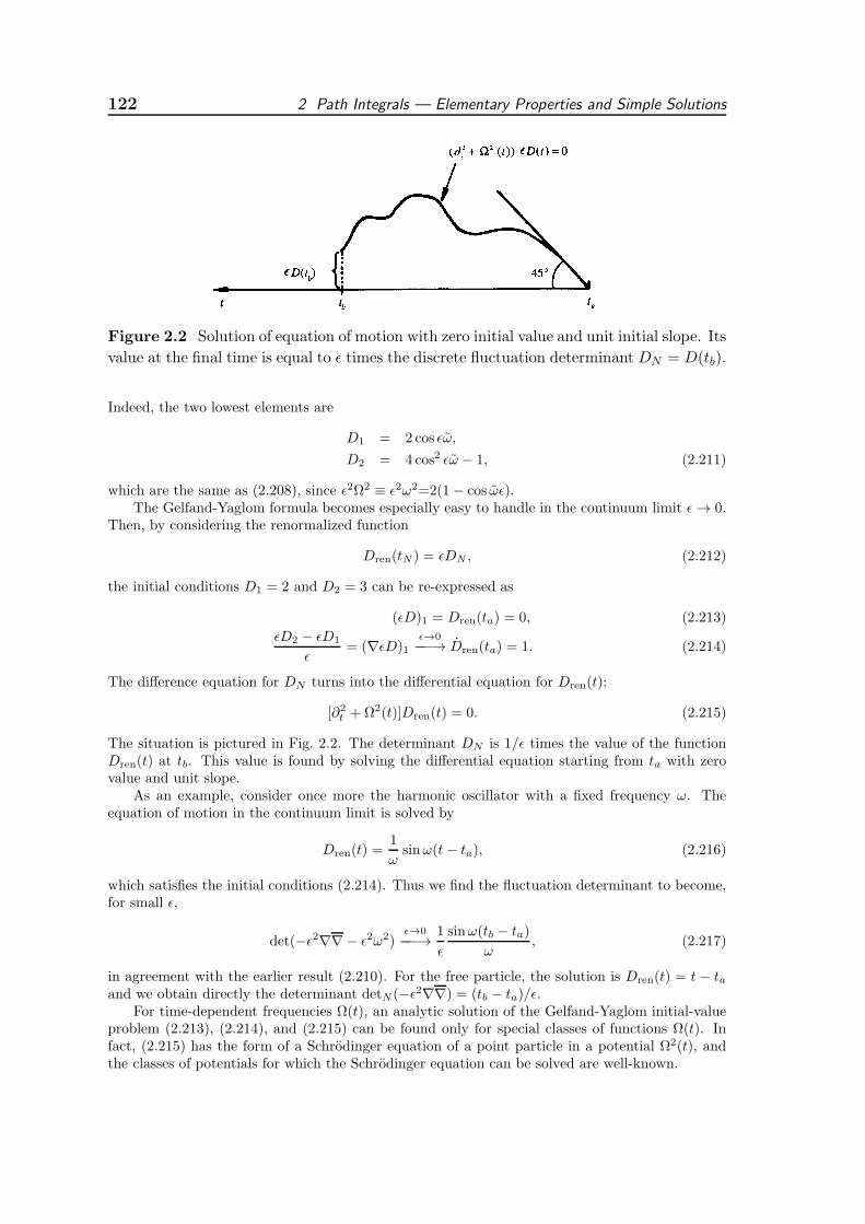
Figure 2.2 Solution of equation of motion with zero initial value and unit initial slope. Its
value at the final time is equal to ǫ times the discrete fluctuation determinant DN = D(tb).
Indeed, the two lowest elements are
D1 = 2 cos ǫω,
D2 = 4 cos2 ǫω − 1, (2.211)
which are the same as (2.208), since ǫ2Ω2 ≡ ǫ2ω2=2(1 − cos ωǫ).The Gelfand-Yaglom formula becomes especially easy to handle in the continuum limit ǫ → 0.
Then, by considering the renormalized function
Dren(tN ) = ǫDN , (2.212)
the initial conditions D1 = 2 and D2 = 3 can be re-expressed as
(ǫD)1 = Dren(ta) = 0, (2.213)
ǫD2 − ǫD1
ǫ= (∇ǫD)1
ǫ→0−−−→ Dren(ta) = 1. (2.214)
The difference equation for DN turns into the differential equation for Dren(t):
[∂2t + Ω2(t)]Dren(t) = 0. (2.215)
The situation is pictured in Fig. 2.2. The determinant DN is 1/ǫ times the value of the functionDren(t) at tb. This value is found by solving the differential equation starting from ta with zerovalue and unit slope.
As an example, consider once more the harmonic oscillator with a fixed frequency ω. Theequation of motion in the continuum limit is solved by
Dren(t) =1
ωsinω(t− ta), (2.216)
which satisfies the initial conditions (2.214). Thus we find the fluctuation determinant to become,for small ǫ,
det(−ǫ2∇∇− ǫ2ω2)ǫ→0−−−→ 1
ǫ
sinω(tb − ta)
ω, (2.217)
in agreement with the earlier result (2.210). For the free particle, the solution is Dren(t) = t− taand we obtain directly the determinant detN (−ǫ2∇∇) = (tb − ta)/ǫ.
For time-dependent frequencies Ω(t), an analytic solution of the Gelfand-Yaglom initial-valueproblem (2.213), (2.214), and (2.215) can be found only for special classes of functions Ω(t). Infact, (2.215) has the form of a Schrodinger equation of a point particle in a potential Ω2(t), andthe classes of potentials for which the Schrodinger equation can be solved are well-known.
2.4 Gelfand-Yaglom Formula 123
2.4.3 Calculation on Unsliced Time Axis
In general, the most explicit way of expressing the solution is by linearly combiningDren=ǫDN from any two independent solutions ξ(t) and η(t) of the homogeneousdifferential equation
[∂2t + Ω2(t)]x(t) = 0. (2.218)
The solution of (2.215) is found from a linear combination
Dren(t) = αξ(t) + βη(t). (2.219)
The coefficients are determined from the initial condition (2.214), which imply
αξ(ta) + βη(ta) = 0,
αξ(ta) + βη(ta) = 1, (2.220)
and thus
Dren(t) =ξ(t)η(ta)− ξ(ta)η(t)
ξ(ta)η(ta)− ξ(ta)η(ta). (2.221)
The denominator is recognized as the time-independent Wronski determinant of thetwo solutions
W ≡ ξ(t)↔
∂ t η(t) ≡ ξ(t)η(t)− ξ(t)η(t) (2.222)
at the initial point ta. The right-hand side is independent of t.The Wronskian is an important quantity in the theory of second-order differential
equations. It is defined for all equations of the Sturm-Liouville type
d
dt
[
a(t)dy(t)
dt
]
+ b(t)y(t) = 0, (2.223)
for which it is proportional to 1/a(t). The Wronskian is used to construct the Greenfunction for all such equations.12
In terms of the Wronskian, Eq. (2.221) has the general form
Dren(t) = − 1
W[ξ(t)η(ta)− ξ(ta)η(t)] . (2.224)
Inserting t = tb gives the desired determinant
Dren = − 1
W[ξ(tb)η(ta)− ξ(ta)η(tb)] . (2.225)
Note that the same functional determinant can be found from by evaluating thefunction
Dren(t) = − 1
W[ξ(tb)η(t)− ξ(t)η(tb)] (2.226)
12For its typical use in classical electrodynamics, see J.D. Jackson, Classical Electrodynamics ,John Wiley & Sons, New York, 1975, Section 3.11.
124 2 Path Integrals — Elementary Properties and Simple Solutions
at ta. This also satisfies the homogenous differential equation (2.215), but with theinitial conditions
Dren(tb) = 0, ˙Dren(tb) = −1. (2.227)
It will be useful to emphasize at which ends the Gelfand-Yaglom boundary condi-tions are satisfied by denoting Dren(t) and Dren(t) by Da(t) and Db(t), respectively,summarizing their symmetric properties as
[∂2t + Ω2(t)]Da(t) = 0 ; Da(ta) = 0, Da(ta) = 1, (2.228)
[∂2t + Ω2(t)]Db(t) = 0 ; Db(tb) = 0, Db(tb) = −1, (2.229)
with the determinant being obtained from either function as
Dren = Da(tb) = Db(ta). (2.230)
In contrast to this we see from the explicit equations (2.224) and (2.226) that thetime derivatives of two functions at opposite endpoints are in general not related.Only for frequencies Ω(t) with time reversal invariance, one has
Da(tb) = −Db(ta), for Ω(t) = Ω(−t). (2.231)
For arbitrary Ω(t), one can derive a relation
Da(tb) + Db(ta) = −2∫ tb
tadtΩ(t)Ω(t)Da(t)Db(t). (2.232)
As an application of these formulas, consider once more the linear oscillator, forwhich two independent solutions are
ξ(t) = cosωt, η(t) = sinωt. (2.233)
Hence
W = ω, (2.234)
and the fluctuation determinant becomes
Dren = − 1
ω(cosωtb sinωta − cosωta sinωtb) =
1
ωsinω(tb − ta). (2.235)
2.4.4 D’Alembert’s Construction
It is important to realize that the construction of the solutions of Eqs. (2.228) and(2.229) requires only the knowledge of one solution of the homogenous differentialequation (2.218), say ξ(t). A second linearly independent solution η(t) can alwaysbe found with the help of a formula due to d’Alembert,
η(t) = w ξ(t)∫ t dt′
ξ2(t′), (2.236)
2.4 Gelfand-Yaglom Formula 125
where w is some constant. Differentiation yields
η =ξη
ξ+w
ξ, η =
ξη
ξ. (2.237)
The second equation shows that with ξ(t), also η(t) is a solution of the homogenousdifferential equation (2.218). From the first equation we find that the Wronskideterminant of the two functions is equal to w:
W = ξ(t)η(t)− ξ(t)η(t) = w. (2.238)
Inserting the solution (2.236) into the formulas (2.224) and (2.226), we obtainexplicit expressions for the Gelfand-Yaglom functions in terms of one arbitrary so-lution of the homogenous differential equation (2.218):
Dren(t)=Da(t)=ξ(t)ξ(ta)∫ t
ta
dt′
ξ2(t′), Dren(t)=Db(t)=ξ(tb)ξ(t)
∫ tb
t
dt′
ξ2(t′). (2.239)
The desired functional determinant is
Dren = ξ(tb)ξ(ta)∫ tb
ta
dt′
ξ2(t′). (2.240)
2.4.5 Another Simple Formula
There exists yet another useful formula for the functional determinant. For this we solve thehomogenous differential equation (2.218) for an arbitrary initial position xa and initial velocityxa at the time ta. The result may be expressed as the following linear combination of Da(t) andDb(t):
x(xa, xa; t) =1
Db(ta)
[
Db(t) −Da(t)Db(ta)]
xa + Da(t)xa . (2.241)
We then see that the Gelfand-Yaglom function Dren(t) = Da(t) can be obtained from the partialderivative
Dren(t) =∂x(xa, xa; t)
∂xa. (2.242)
This function obviously satisfies the Gelfand-Yaglom initial conditions Dren(ta) = 0 and Dren(ta) =1 of (2.213) and (2.214), which are a direct consequence of the fact that xa and xa are independentvariables in the function x(xa, xa; t), for which ∂xa/∂xa = 0 and ∂xa/∂xa = 1.
The fluctuation determinant Dren = Da(tb) is then given by
Dren =∂xb
∂xa, (2.243)
where xb abbreviates the function x(xa, xa; tb). It is now obvious that the analogous equations(2.229) are satisfied by the partial derivative Db(t) = −∂x(t)/∂xb, where x(t) is expressed in termsof the final position xb and velocity xb as x(t) = x(xb, xb; t)
x(xb, xb; t) =1
Da(tb)
[
Da(t) + Db(t)Da(tb)]
xb −Db(t)xb , (2.244)
126 2 Path Integrals — Elementary Properties and Simple Solutions
so that we obtain the alternative formula
Dren = −∂xa
∂xb. (2.245)
These results can immediately be generalized to functional determinants of differential opera-tors of the form −∂2
t δij−Ω2ij(t) where the time-dependent frequency is a D×D-dimensional matrix
Ω2ij(t), (i, j = 1, . . . , D). Then the associated Gelfand-Yaglom function Da(t) becomes a matrix
Dij(t) satisfying the initial conditions Dij(ta) = 0, Dij(tb) = δij , and the desired functionaldeterminant Dren is equal to the ordinary determinant of Dij(tb):
Dren = Det[
−∂2t δij − Ω2
ij(t)]
= detDij(tb). (2.246)
The homogeneous differential equation and the initial conditions are obviously satisfied by thepartial derivative matrix Dij(t) = ∂xi(t)/∂xj
a, so that the explicit representations of Dij(t) interms of the general solution of the classical equations of motion
[
−∂2t δij − Ω2
ij(t)]
xj(t) = 0become
Dren = det∂xi
b
∂xja
= det
(
−∂xia
∂xjb
)
. (2.247)
A further couple of formulas for functional determinants can be found by constructing a solutionof the homogeneous differential equation (2.218) which passes through specific initial and finalpoints xa and xb at ta and tb, respectively:
x(xb, xa; t) =Db(t)
Db(ta)xa +
Da(t)
Da(tb)xb. (2.248)
The Gelfand-Yaglom functions Da(t) and Db(t) can therefore be obtained from the partial deriva-tives
Da(t)
Da(tb)=
∂x(xb, xa; t)
∂xb,
Db(t)
Db(ta)=
∂x(xb, xa; t)
∂xa. (2.249)
At the endpoints, Eqs. (2.248) yield
xa =Db(ta)
Db(ta)xa +
1
Da(tb)xb, (2.250)
xb = − 1
Db(ta)xa +
Da(tb)
Da(tb)xb, (2.251)
so that the fluctuation determinant Dren = Da(tb) = Db(ta) is given by the formulas
Dren =
(
∂xa
∂xb
)−1
= −(
∂xb
∂xa
)−1
, (2.252)
where xa and xb are functions of the independent variables xa and xb. The equality of these ex-pressions with the previous ones in (2.243) and (2.245) is a direct consequence of the mathematicalidentity for partial derivatives
∂xb
∂xa
∣
∣
∣
∣
xa
=
(
∂xa
∂xb
∣
∣
∣
∣
xa
)−1
. (2.253)
Let us emphasize that all functional determinants calculated in this Chapter apply to thefluctuation factor of paths with fixed endpoints. In mathematics, this property is referred toas Dirichlet boundary conditions. In the context of quantum statistics, we shall also need suchdeterminants for fluctuations with periodic boundary conditions, for which the Gelfand-Yaglommethod must be modified. We shall see in Section 2.11 that this causes considerable complications
2.5 Harmonic Oscillator with Time-Dependent Frequency 127
in the lattice derivation, which will make it desirable to find a simpler derivation of both functionaldeterminants. This will be found in Section 3.27 in a continuum formulation.
In general, the homogenous differential equation (2.218) with time-dependent frequency Ω(t)cannot be solved analytically. The equation has the same form as a Schrodinger equation fora point particle in one dimension moving in a one dimensional potential Ω2(t), and there areonly a few classes of potentials for which the solutions are known in closed form. Fortunately,however, the functional determinant will usually arise in the context of quadratic fluctuationsaround classical solutions in time-independent potentials (see in Section 4.3). If such a classicalsolution is known analytically, it will provide us automatically with a solution of the homogeneousdifferential equation (2.218). Some important examples will be discussed in Sections 17.4 and17.11.
2.4.6 Generalization to D Dimensions
The above formulas have an obvious generalization to a D-dimensional version ofthe fluctuation action (2.201)
A =∫ tb
tadtM
2[(δx)2 − δxT
2(t)δx], (2.254)
where 2(t) is a D×D matrix with elements Ω2ij(t). The fluctuation factor (2.202)
generalizes to
FN(tb, ta) =1
√
2πhi(tb − ta)/MD
[
detN (−ǫ2∇∇− ǫ22)
detN(−ǫ2∇∇)
]−1/2
. (2.255)
The fluctuation determinant is found by Gelfand-Yaglom’s construction from a for-mula
Dren = detDa(tb) = detDb(ta), (2.256)
with the matrices Da(t) and Db(t) satisfying the classical equations of motion andinitial conditions corresponding to (2.228) and (2.229):
[∂2t +2(t)]Da(t) = 0 ; Da(ta) = 0, Da(ta) = 1, (2.257)
[∂2t +2(t)]Db(t) = 0 ; Db(tb) = 0, Db(tb) = −1, (2.258)
where 1 is the unit matrix in D dimensions. We can then repeat all steps in the lastsection and find the D-dimensional generalization of formulas (2.252):
Dren =
(
det∂xia∂xjb
)−1
=
[
det
(
−∂xib
∂xja
)]−1
. (2.259)
2.5 Harmonic Oscillator with Time-Dependent Frequency
The results of the last section put us in a position to solve exactly the path integralof a harmonic oscillator with arbitrary time-dependent frequency Ω(t). We shallfirst do this in coordinate space, later in momentum space.
128 2 Path Integrals — Elementary Properties and Simple Solutions
2.5.1 Coordinate Space
Consider the path integral
(xbtb|xata) =∫
Dx exp
i
hA[x]
, (2.260)
with the Lagrangian action
A[x] =M
2
∫ tb
tadt[
x2(t)− Ω2(t)x2(t)]
, (2.261)
which is harmonic with a time-dependent frequency. As in Eq. (2.14), the result canbe written as a product of a fluctuation factor and an exponential containing theclassical action:
(xbtb|xata) =∫
Dx eiA[x]/h = FΩ(tb, ta)eiAcl/h. (2.262)
From the discussion in the last section we know that the fluctuation factor is, byanalogy with (2.171), and recalling (2.243),
FΩ(tb, ta) =1
√
2πih/M
1√
Da(tb). (2.263)
The determinant Da(tb) = Dren may be expressed in terms of partial derivativesaccording to formulas (2.243) and (2.252):
FΩ(tb, ta) =1
√
2πih/M
(
∂xb∂xa
)−1/2
=1
√
2πih/M
(
∂xa∂xb
)1/2
, (2.264)
where the first partial derivative is calculated from the function x(xa, xa; t), thesecond from x(xb, xa; t). Equivalently we may use (2.245) and the right-hand partof Eq. (2.252) to write
FΩ(tb, ta) =1
√
2πih/M
(
−∂xa∂xb
)−1/2
=1
√
2πih/M
(
−∂xb∂xa
)1/2
. (2.265)
It remains to calculate the classical action Acl. This can be done in the sameway as in Eqs. (2.155) to (2.159). After a partial integration, we have as before
Acl =M
2(xbxb − xaxa). (2.266)
Exploiting the linear dependence of xb and xa on the endpoints xb and xa, we mayrewrite this as
Acl =M
2
(
xb∂xb∂xb
xb − xa∂xa∂xa
xa + xb∂xb∂xa
xa − xa∂xa∂xb
xb
)
. (2.267)
2.5 Harmonic Oscillator with Time-Dependent Frequency 129
Inserting the partial derivatives from (2.250) and (2.251) and using the equality ofDa(tb) and Db(ta), we obtain the classical action
Acl =M
2Da(tb)
[
x2bDa(tb)− x2aDb(ta)− 2xbxa]
. (2.268)
Note that there exists another simple formula for the fluctuation determinant Dren:
Dren = Da(tb) = Db(ta) = −M(
∂2
∂xb∂xaAcl
)−1
. (2.269)
For the harmonic oscillator with time-independent frequency ω, the Gelfand-Yaglom function Da(t) of Eq. (2.235) has the property (2.231) due to time reversalinvariance, and (2.268) reproduces the known result (2.159).
The expressions containing partial derivatives are easily extended to D dimen-sions: We simply have to replace the partial derivatives ∂xb/∂xa, ∂xb/∂xa, . . . bythe corresponding D×D matrices, and write the action as the associated quadraticform.
The D-dimensional versions of the fluctuation factors (2.264) are
FΩ(tb, ta) =1
√
2πih/MD
[
det∂xib∂xja
]−1/2
=1
√
2πih/MD
[
det∂xia∂xjb
]1/2
. (2.270)
All formulas for fluctuation factors hold initially only for sufficiently short timestb − ta. For larger times, they carry phase factors determined as before in (2.169).The fully defined expression may be written as
FΩ(tb, ta) =1
√
2πih/MD
∣
∣
∣
∣
∣
det∂xib∂xja
∣
∣
∣
∣
∣
−1/2
e−iνπ/2 =1
√
2πih/MD
∣
∣
∣
∣
∣
det∂xia∂xjb
∣
∣
∣
∣
∣
1/2
e−iνπ/2,
(2.271)where ν is the Maslov-Morse index. In the one-dimensional case it counts the turn-ing points of the trajectory, in the multidimensional case the number of zeros indeterminant det ∂xib/∂x
ja along the trajectory, if the zero is caused by a reduction
of the rank of the matrix ∂xib/∂xja by one unit. If it is reduced by more than one
unit, ν increases accordingly. In this context, the number ν is also called the Morse
index of the trajectory.The zeros of the functional determinant are also called conjugate points . They
are generalizations of the turning points in one-dimensional systems. The surfacesin x-space, on which the determinant vanishes, are called caustics . The conjugatepoints are the places where the orbits touch the caustics.13
Note that for infinitesimally short times, all fluctuation factors and classical ac-tions coincide with those of a free particle. This is obvious for the time-independentharmonic oscillator, where the amplitude (2.177) reduces to that of a free particle
13See M.C. Gutzwiller, Chaos in Classical and Quantum Mechanics , Springer, Berlin, 1990.
130 2 Path Integrals — Elementary Properties and Simple Solutions
in Eq. (2.74) in the limit tb → ta. Since a time-dependent frequency is constant overan infinitesimal time, this same result holds also here. Expanding the solution ofthe equations of motion for infinitesimally short times as
xb ≈ (tb − ta)xa + xa, xa ≈ −(tb − ta)xb + xb, (2.272)
we have immediately
∂xib∂xja
= δij(tb − ta),∂xa
∂xjb= −δij(tb − ta). (2.273)
Similarly, the expansions
xb ≈ xa ≈xb − xa
tb − ta(2.274)
lead to
∂xib∂xja
= −δij1
tb − ta,
∂xia∂xjb
= δij1
tb − ta. (2.275)
Inserting the expansions (2.273) or (2.274) into (2.266) (in D dimensions), the actionreduces approximately to the free-particle action
Acl ≈M
2
(xb − xa)2
tb − ta. (2.276)
2.5.2 Momentum Space
Let us also find the time evolution amplitude in momentum space. For this we write the classicalaction (2.267) as a quadratic form
Acl =M
2(xb, xa)A
(
xb
xa
)
(2.277)
with a matrix
A =
∂xb
∂xb
∂xb
∂xa
−∂xa
∂xb−∂xa
∂xa
. (2.278)
The inverse of this matrix is
A−1 =
∂xb
∂xb− ∂xb
∂xa
∂xa
∂xb−∂xa
∂xa
. (2.279)
The partial derivatives of xb and xa are calculated from the solution of the homogeneous differentialequation (2.218) specified in terms of the final and initial velocities xb and xa:
x(xb, xa; t) =1
Da(tb)Db(ta) + 1
×[
Da(t) + Db(t)Da(tb)]
xa +[
−Db(t) + Da(t)Db(ta)]
xb
, (2.280)

2.5 Harmonic Oscillator with Time-Dependent Frequency 131
which yields
xa =1
Da(tb)Db(ta) + 1
[
Db(ta)Da(ta)xb −Db(ta)xb
]
, (2.281)
xb =1
Da(tb)Db(ta) + 1
[
Da(tb)xa + Da(tb)Db(ta)xb
]
, (2.282)
so that
A−1 =Da(tb)
Da(tb)Db(ta) + 1
Db(ta) −1
−1 −Da(tb)
. (2.283)
The determinant of A is the Jacobian
detA = −∂(xb, xa)
∂(xb, xa)= − Da(tb)Db(ta) + 1
Da(tb)Db(ta). (2.284)
We can now perform the Fourier transform of the time evolution amplitude and find, via a quadraticcompletion,
(pbtb|pata) =
∫
dxb e−ipbxb/h
∫
dxa eipaxa/h(xbtb|xata) (2.285)
=
√
2πh
iM
√
Da(tb)
Da(tb)Db(ta) + 1
× exp
i
h
1
2M
Da(tb)
Da(tb)Db(ta) + 1
[
−Db(ta)p2b + Da(tb)p
2a − 2pbpa
]
.
Inserting here Da(tb) = sinω(tb− ta)/ω and Da(tb) = cosω(tb− ta), we recover the oscillator result(2.189).
In D dimensions, the classical action has the same quadratic form as in (2.277)
Acl =M
2
(
xTb ,x
Ta
)
A
(
xb
xa
)
(2.286)
with a matrix A generalizing (2.278) by having the partial derivatives replaced by the correspondingD ×D-matrices. The inverse is the 2D × 2D-version of (2.279), i.e.
A =
∂xb
∂xb
∂xb
∂xa
−∂xa
∂xb−∂xa
∂xa
, A−1 =
∂xb
∂xb− ∂xb
∂xa
∂xa
∂xb−∂xa
∂xa
. (2.287)
The determinant of such a block matrix
A =
(
a bc d
)
(2.288)
is calculated after a triangular decomposition
A =
(
a bc d
)
=
(
a 0c 1
)(
1 a−1b0 d− ca−1b
)
=
(
1 b0 d
)(
a− bd−1c 0d−1c 1
)
(2.289)
in two possible ways as
det
(
a bc d
)
= det a · det (d− ca−1b) = det (a− bd−1c) · det d, (2.290)
132 2 Path Integrals — Elementary Properties and Simple Solutions
depending whether det a or det b is nonzero. The inverse is in the first case
A=
(
1 −a−1bx0 x
)(
a−1 0−ca−1 1
)
=
(
a−1+a−1bxca−1−a−1bx−xca−1 x
)
, x≡(d−ca−1b)−1. (2.291)
The resulting amplitude in momentum space is
(pbtb|pata) =
∫
dxb e−ipbxb/h
∫
dxa eipaxa/h(xbtb|xata)
=2π√
2πihM
1√DrendetA
exp
i
h
1
2M
[
(
pTb ,p
Ta
)
A−1
(
pb
pa
)]
. (2.292)
Also in momentum space, the amplitude (2.292) reduces to the free-particle one in Eq. (2.73)in the limit of infinitesimally short time tb− ta: For the time-independent harmonic oscillator, thiswas shown in Eq. (2.191), and the time-dependence of Ω(t) becomes irrelevant in the limit of smalltb − ta → 0.
2.6 Free-Particle and Oscillator Wave Functions
In Eq. (1.335) we have expressed the time evolution amplitude of the free particle(2.72) as a Fourier integral
(xbtb|xata) =∫
dp
(2πh)eip(xb−xa)/he−ip2(tb−ta)/2Mh. (2.293)
This expression contains the information on all stationary states of the system. Tofind these states we have to perform a spectral analysis of the amplitude. Recallthat according to Section 1.7, the amplitude of an arbitrary time-independent systempossesses a spectral representation of the form
(xbtb|xata) =∞∑
n=0
ψn(xb)ψ∗n(xa)e
−iEn(tb−ta)/h, (2.294)
where En are the eigenvalues and ψn(x) the wave functions of the stationary states.In the free-particle case the spectrum is continuous and the spectral sum is anintegral. Comparing (2.294) with (2.293) we see that the Fourier decompositionitself happens to be the spectral representation. If the sum over n is written as anintegral over the momenta, we can identify the wave functions as
ψp(x) =1√2πh
eipx. (2.295)
For the time evolution amplitude of the harmonic oscillator
(xbtb|xata) =1
√
2πih sin [ω(tb − ta)] /Mω(2.296)
× exp
iMω
2h sin [ω(tb − ta)]
[
(x2b + x2a) cosω(tb − ta)− 2xbxa]
,
2.6 Free-Particle and Oscillator Wave Functions 133
the procedure is not as straight-forward. Here we must make use of a summationformula for Hermite polynomials (see Appendix 2C) Hn(x) due to Mehler:14
1√1− a2
exp
− 1
2(1− a2)[(x2 + x′2)(1 + a2)− 4xx′a]
= exp(−x2/2− x′2/2)∞∑
n=0
an
2nn!Hn(x)Hn(x
′), (2.297)
with
H0(x) = 1, H1(x) = 2x, H2(x) = 4x2 − 2, . . . , Hn(x) = (−1)nex2 dn
dxne−x2
. (2.298)
Identifying
x ≡√
Mω/h xb, x′ ≡√
Mω/h xa, a ≡ e−iω(tb−ta), (2.299)
so that
a
1− a2=
1
2i sin [ω(tb − ta)],
1 + a2
1− a2=
1 + e−2iω(tb−ta)
1− e−2iω(tb−ta)=
cos [ω(tb − ta)]
i sin [ω(tb − ta)]
we arrive at the spectral representation
(xbtb|xata) =∞∑
n=0
ψn(xb)ψn(xa)e−i(n+1/2)ω(tb−ta). (2.300)
From this we deduce that the harmonic oscillator has the energy eigenvalues
En = hω(n+ 1/2) (2.301)
and the wave functions
ψn(x) = Nnλ−1/2ω e−x2/2λ2
ωHn(x/λω). (2.302)
Here, λω is the natural length scale of the oscillator
λω ≡√
h
Mω, (2.303)
and Nn the normalization constant
Nn = (1/2nn!√π)1/2. (2.304)
It is easy to check that the wave functions satisfy the orthonormality relation∫ ∞
−∞dxψn(x)ψn′(x)∗ = δnn′, (2.305)
using the well-known orthogonality relation of Hermite polynomials15
1
2nn!√π
∫ ∞
−∞dx e−x2
Hn(x)Hn′(x) = δn,n′. (2.306)
14See P.M. Morse and H. Feshbach, Methods of Theoretical Physics , McGraw-Hill, New York,Vol. I, p. 781 (1953).
15I.S. Gradshteyn and I.M. Ryzhik, op. cit., Formula 7.374.1.
134 2 Path Integrals — Elementary Properties and Simple Solutions
2.7 General Time-Dependent Harmonic Action
A simple generalization of the harmonic oscillator with time-dependent frequency allows also fora time-dependent mass, so that the action (2.307) becomes
A[x] =
∫ tb
ta
dtM
2
[
g(t)x2(t) − Ω2(t)x2(t)]
, (2.307)
with some dimensionless time-dependent factor g(t). This factor changes the measure of pathintegration so that the time evolution amplitude can no longer be calculated from (2.260). To findthe correct measure we must return to the canonical path integral (2.29) which now reads
(xbtb|xata) =
∫ x(tb)=xb
x(ta)=xa
D′x
∫ Dp
2πheiA[p,x]/h, (2.308)
with the canonical action
A[p, x] =
∫ tb
ta
dt
[
px− p2
2Mg(t)− M
2Ω2(t)x2(t)
]
. (2.309)
Integrating the momentum variables out in the sliced form of this path integral as in Eqs. (2.51)–(2.53) yields
(xbtb|xata) ≈1
√
2πhiǫ/Mg(tN+1)
N∏
n=1
[
∫ ∞
−∞
dxn√
2πhiǫ/Mg(tn)
]
exp
(
i
hAN
)
. (2.310)
The continuum limit of this path integral is written as
(xbtb|xata) =
∫
Dx√g exp
i
hA[x]
, (2.311)
with the action (2.307).The classical orbits solve the equation of motion
[
−∂tg(t)∂t − Ω2(t)]
x(t) = 0, (2.312)
which, by the transformation
x(t) =√
g(t)x(t), Ω2(t) =1
g(t)
[
Ω2(t) +g2(t)
4g(t)− g(t)
2
]
, (2.313)
can be reduced to the previous form
√
g(t)[
−∂2t − Ω2(t)
]
x(t) = 0. (2.314)
The result of the path integration is therefore
(xbtb|xata) =
∫
Dx√g eiA[x]/h = F (xb, tb;xa, ta)e
iAcl/h, (2.315)
with a fluctuation factor [compare (2.263)]
F (xb, tb;xa, ta) =1
√
2πih/M
1√
Da(tb), (2.316)
where Da(tb) is found from a generalization of the formulas (2.264)–(2.269). The classical actionis
Acl =M
2(gbxbxb − gaxaxa), (2.317)
2.8 Path Integrals and Quantum Statistics 135
where gb ≡ g(tb), ga ≡ g(ta). The solutions of the equation of motion can be expressed in termsof modified Gelfand-Yaglom functions (2.228) and (2.229) with the properties
[∂tg(t)∂t + Ω2(t)]Da(t) = 0 ; Da(ta) = 0, Da(ta) = 1/ga, (2.318)
[∂tg(t)∂t + Ω2(t)]Db(t) = 0 ; Db(tb) = 0, Db(tb) = −1/gb, (2.319)
as in (2.248):
x(xb, xa; t) =Db(t)
Db(ta)xa +
Da(t)
Da(tb)xb. (2.320)
This allows us to write the classical action (2.317) in the form
Acl =M
2Da(tb)
[
gbx2bDa(tb) − gax
2aDb(ta) − 2xbxa
]
. (2.321)
From this we find, as in (2.269),
Dren = Da(tb) = Db(ta) = −M
(
∂2Acl
∂xb∂xa
)−1
, (2.322)
so that the fluctuation factor becomes
F (xb, tb;xa, ta) =1√
2πih
√
− ∂2Acl
∂xb∂xa. (2.323)
As an example take a free particle with a time-dependent mass term, where
Da(t)=
∫ t
ta
dt′ g−1(t′), Db(t)=
∫ tb
t
dt′ g−1(t′), Dren=Da(tb)=Db(ta)=
∫ tb
ta
dt′ g−1(t′), (2.324)
and the classical action reads
Acl =M
2
(xb − xa)2
Da(tb). (2.325)
The result can easily be generalized to an arbitrary harmonic action
A =
∫ tb
ta
dtM
2
[
g(t)x2 + 2b(t)xx− Ω2(t)x2]
, (2.326)
which is extremized by the Euler-Lagrange equation [recall (1.8)][
∂tg(t)∂t + b(t) + Ω2(t)]
x = 0. (2.327)
The solution of the path integral (2.315) is again given by (2.315), with the fluctuation factor(2.323), where Acl is the action (2.326) along the classical path connecting the endpoints.
A further generalization to D dimensions is obvious by adapting the procedure in Subsec-tion 2.4.6, which makes Eqs. (2.318)–(2.320). matrix equations.
2.8 Path Integrals and Quantum Statistics
The path integral approach is useful to also understand the thermal equilibriumproperties of a system. We assume the system to have a time-independent Hamilto-nian and to be in contact with a reservoir of temperature T . As explained in Sec-tion 1.7, the bulk thermodynamic quantities can be determined from the quantum-statistical partition function
Z = Tr(
e−H/kBT)
=∑
n
e−En/kBT . (2.328)
136 2 Path Integrals — Elementary Properties and Simple Solutions
This, in turn, may be viewed as an analytic continuation of the quantum-mechanicalpartition function
ZQM = Tr(
e−i(tb−ta)H/h)
(2.329)
to the imaginary time
tb − ta = − ih
kBT≡ −ihβ. (2.330)
In the local particle basis |x〉, the quantum-mechanical trace corresponds to anintegral over all positions so that the quantum-statistical partition function can beobtained by integrating the time evolution amplitude over xb = xa and evaluatingit at the analytically continued time:
Z ≡∫ ∞
−∞dx z(x) =
∫ ∞
−∞dx 〈x|e−βH |x〉 =
∫ ∞
−∞dx (x tb|x ta)|tb−ta=−ihβ. (2.331)
The diagonal elements
z(x) ≡ 〈x|e−βH |x〉 = (x tb|x ta)|tb−ta=−ihβ (2.332)
play the role of a partition function density . For a harmonic oscillator, this quantityhas the explicit form [recall (2.175)]
zω(x) =1
√
2πh/M
√
ω
sinh hβωexp
(
−Mω
htanh
hβω
2x2)
. (2.333)
By splitting the Boltzmann factor e−βH into a product of N + 1 factors e−ǫH/h
with ǫ = h/kBT (N + 1), we can derive for Z a similar path integral representa-tion just as for the corresponding quantum-mechanical partition function in (2.42),(2.48):
Z ≡N+1∏
n=1
[∫ ∞
−∞dxn
]
(2.334)
× 〈xN+1|e−ǫH/h|xN〉〈xN |e−ǫH/h|xN−1〉 × . . .× 〈x2|e−ǫH/h|x1〉〈x1|e−ǫH/h|xN+1〉.
As in the quantum-mechanical case, the matrix elements 〈xn|e−ǫH/h|xn−1〉 are re-expressed in the form
〈xn|e−ǫH/h|xn−1〉 ≈∫ ∞
−∞
dpn2πh
eipn(xn−xn−1)/h−ǫH(pn,xn)/h, (2.335)
with the only difference that there is now no imaginary factor i in front of theHamiltonian. The product (2.334) can thus be written as
Z ≈N+1∏
n=1
[
∫ ∞
−∞dxn
∫ ∞
−∞
dpn2πh
]
exp(
−1
hAN
e
)
, (2.336)

2.8 Path Integrals and Quantum Statistics 137
where ANe denotes the sum
ANe =
N+1∑
n=1
[−ipn(xn − xn−1) + ǫH(pn, xn)] . (2.337)
In the continuum limit ǫ→ 0, the sum goes over into the integral
Ae[p, x] =∫ hβ
0dτ [−ip(τ)x(τ) +H(p(τ), x(τ))], (2.338)
and the partition function is given by the path integral
Z =∫
Dx∫ Dp
2πhe−Ae[p,x]/h. (2.339)
In this expression, p(τ), x(τ) may be considered as paths running along an “imag-inary time axis” τ = it. The expression Ae[p, x] is very similar to the mechanicalcanonical action (2.27). Since it governs the quantum-statistical path integrals itis called quantum-statistical action or Euclidean action, indicated by the subscripte. The name alludes to the fact that a D-dimensional Euclidean space extendedby an imaginary-time axis τ = it has the same geometric properties as a D + 1-dimensional Euclidean space. For instance, a four-vector in a Minkowski spacetimehas a square length dx2 = −(cdt)2 + (dx)2. Continued to an imaginary time, thisbecomes dx2 = (cdτ)2 + (dx)2 which is the square distance in a Euclidean four-dimensional space with four-vectors (cτ,x).
The integrand of the Euclidean action (2.339) is the Euclidean Lagrangian Le. Itis related to the Hamiltonian by the Euclidean Legendre transform [compare (1.9)]
H = Le + i∂Le
∂xx = Le + ipx (2.340)
in which x is eliminated in favor of p = ∂Le/∂x [compare (1.10)].Just as in the path integral for the quantum-mechanical partition function (2.48),
the measure of integration∮ Dx ∫ Dp/2πh in the quantum-statistical expression
(2.339) is automatically symmetric in all p’s and x’s:
∮
Dx∫ Dp
2πh=∮ Dp
2πh
∫
Dx =N+1∏
n=1
∫ ∞
−∞dxn
∫ ∞
−∞
dpn2πh
. (2.341)
The symmetry is of course due to the trace integration over all initial ≡ final posi-tions.
Most remarks made in connection with Eq. (2.48) carry over to the presentcase. The above path integral (2.339) is a natural extension of the rules of clas-sical statistical mechanics. According to these, each cell in phase space dxdp/h isoccupied with equal statistical weight, with the probability factor e−E/kBT . In quan-tum statistics, the paths of all particles fluctuate evenly over the cells in path phase
space∏
n dx(τn)dp(τn)/h (τn ≡ nǫ), each path carrying a probability factor e−Ae/h
involving the Euclidean action of the system.
138 2 Path Integrals — Elementary Properties and Simple Solutions
2.9 Density Matrix
The partition function does not determine any local thermodynamic quantities. Im-portant local information resides in the thermal analog of the time evolution ampli-tude 〈xb|e−H/kBT |xa〉. Consider, for instance, the diagonal elements of this amplituderenormalized by a factor Z−1:
ρ(xa) ≡ Z−1〈xa|e−H/kBT |xa〉. (2.342)
They determine the thermal average of the particle density of a quantum-statisticalsystem. Due to (2.334), the factor Z−1 makes the spatial integral over ρ equal tounity:
∫ ∞
−∞dx ρ(x) = 1. (2.343)
By inserting into (2.342) a complete set of eigenfunctions ψn(x) of the Hamiltonianoperator H, we find the spectral decomposition
ρ(xa) =∑
n
|ψn(xa)|2e−βEn
/
∑
n
e−βEn. (2.344)
Since |ψn(xa)|2 is the probability distribution of the system in the eigenstate |n〉,while the ratio e−βEn/
∑
n e−βEn is the normalized probability to encounter the sys-
tem in the state |n〉, the quantity ρ(xa) represents the normalized average particledensity in space as a function of temperature.
Note the limiting properties of ρ(xa). In the limit T → 0, only the lowest energystate survives and ρ(xa) tends towards the particle distribution in the ground state
ρ(xa)T→0−−−→ |ψ0(xa)|2. (2.345)
In the opposite limit of high temperatures, quantum effects are expected to becomeirrelevant and the partition function should converge to the classical expression(1.538) which is the integral over the phase space of the Boltzmann distribution
ZT→∞−−−→ Zcl =
∫ ∞
−∞dx∫ ∞
−∞
dp
2πhe−H(p,x)/kBT . (2.346)
We therefore expect the large-T limit of ρ(x) to be equal to the classical particle
distribution
ρ(x)T→∞−−−→ ρcl(x) = Z−1
cl
∫ ∞
−∞
dp
2πhe−H(p,x)/kBT . (2.347)
Within the path integral approach, this limit will be discussed in more detail inSection 2.13. At this place we roughly argue as follows: When going in the originaltime-sliced path integral (2.334) to large T , i.e., small τb − τa = h/kBT , we maykeep only a single time slice and write
Z ≈[∫ ∞
−∞dx]
〈x|e−ǫH/h|x〉, (2.348)
2.9 Density Matrix 139
with
〈x|e−ǫH |x〉 ≈∫ ∞
−∞
dpn2πh
e−ǫH(pn,x)/h. (2.349)
After substituting ǫ = τb − τa this gives directly (2.347). Physically speaking, thepath has at high temperatures “no (imaginary) time” to fluctuate, and only oneterm in the product of integrals needs to be considered.
If H(p, x) has the standard form
H(p, x) =p2
2M+ V (x), (2.350)
the momentum integral is Gaussian in p and can be done using the formula∫ ∞
−∞
dp
2πhe−ap2/2h =
1√2πha
. (2.351)
This leads to the pure x-integral for the classical partition function
Zcl =∫ ∞
−∞
dx√
2πh2/MkBTe−V (x)/kBT =
∫ ∞
−∞
dx
le(hβ)e−βV (x). (2.352)
In the second expression we have introduced the length
le(hβ) ≡√
2πh2β/M. (2.353)
It is the thermal (or Euclidean) analog of the characteristic length l(tb − ta) intro-duced before in (2.131). It is called the deBroglie wavelength associated with the
temperature T = 1/kBβ or, in short, the thermal de Broglie wavelength.Omitting the x-integration in (2.352) renders the large-T limit ρ(x), the classical
particle distribution
ρ(x)T→∞−−−→ ρcl(x) = Z−1
cl
1
le(hβ)e−V (x). (2.354)
For a free particle, the integral over x in (2.352) diverges. If we imagine the lengthof the x-axis to be very large but finite, say equal to L, the partition function isequal to
Zcl =L
le(hβ). (2.355)
In D dimensions, this becomes
Zcl =VD
lDe (hβ), (2.356)
where VD is the volume of the D-dimensional system. For a harmonic oscillatorwith potential Mω2x2/2, the integral over x in (2.352) is finite and yields, in theD-dimensional generalization
Zcl =lDω
lD(hβ), (2.357)
140 2 Path Integrals — Elementary Properties and Simple Solutions
where
lω ≡√
2π
βMω2(2.358)
denotes the classical length scale defined by the frequency of the harmonic oscillator.It is related to the quantum-mechanical one λω of Eq. (2.303) by
lω le(hβ) = 2π λ2ω. (2.359)
Thus we obtain the mnemonic rule for going over from the partition function of aharmonic oscillator to that of a free particle: we must simply replace
lω −−−→ω→0
L, (2.360)
or1
ω−−−→ω→0
√
βM
2πL. (2.361)
The real-time version of this is, of course,
1
ω−−−→ω→0
√
(tb − ta)M
2πhL. (2.362)
Let us write down a path integral representation for ρ(x). Omitting in (2.339)the final trace integration over xb ≡ xa and normalizing the expression by a factorZ−1, we obtain
ρ(xa) = Z−1∫ x(hβ)=xb
x(0)=xa
D′x∫ Dp
2πhe−Ae[p,x]/h
= Z−1∫ x(hβ)=xb
x(0)=xa
Dxe−Ae[x]/h. (2.363)
The thermal equilibrium expectation of an arbitrary Hermitian operator O isgiven by
〈O〉T ≡ Z−1∑
n
e−βEn〈n|O|n〉. (2.364)
In the local basis |x〉, this becomes
〈O〉T = Z−1∫∫ ∞
−∞dxbdxa〈xb|e−βH |xa〉〈xa|O|xb〉. (2.365)
An arbitrary function of the position operator x has the expectation
〈f(x)〉T = Z−1∫∫ ∞
−∞dxbdxa〈xb|e−βH |xa〉δ(xb − xa)f(xa) =
∫
dxρ(x)f(x). (2.366)
The particle density ρ(xa) determines the thermal averages of local observables.If f depends also on the momentum operator p, then the off-diagonal matrix
elements 〈xb|e−βH |xa〉 are also needed. They are contained in the density matrix
2.9 Density Matrix 141
introduced for pure quantum systems in Eq. (1.221), and reads now in a thermalensemble of temperature T :
ρ(xb, xa) ≡ Z−1〈xb|e−βH |xa〉, (2.367)
whose diagonal values coincide with the above particle density ρ(xa).It is useful to keep the analogy between quantum mechanics and quantum statis-
tics as close as possible and to introduce the time translation operator along theimaginary time axis
Ue(τb, τa) ≡ e−(τb−τa)H/h, τb > τa, (2.368)
defining its local matrix elements as imaginary or Euclidean time evolutionamplitudes16
(xbτb|xaτa) ≡ 〈xb|Ue(τb, τa)|xa〉, τb > τa. (2.369)
As in the real-time case, we shall only consider the causal time-ordering τb > τa.Otherwise the partition function and the density matrix do not exist in systems withenergies up to infinity. Given the imaginary-time amplitudes, the partition functionis found by integrating over the diagonal elements
Z =∫ ∞
−∞dx(x hβ|x 0), (2.370)
and the density matrix
ρ(xb, xa) = Z−1(xbhβ|xa0). (2.371)
For the sake of generality we may sometimes also consider the imaginary-timeevolution operators for time-dependent Hamiltonians and the associated amplitudes.They are obtained by time-slicing the local matrix elements of the operator
U(τb, τa) = Tτ exp[
−1
h
∫ τb
τadτH(−iτ)
]
. (2.372)
Here Tτ is an ordering operator along the imaginary-time axis.It must be emphasized that the usefulness of the operator (2.372) in describing
thermodynamic phenomena is restricted to the Hamiltonian operator H(t) depend-ing very weakly on the physical time t. The system has to remain close to equilibriumat all times. This is the range of validity of the so-called linear response theory (seeChapter 18 for more details).
The imaginary-time evolution amplitude (2.369) has a path integral representa-tion which is obtained by dropping the final integration in (2.336) and relaxing thecondition xb = xa:
(xbτb|xaτa) ≈N∏
n=1
[∫ ∞
−∞dxn
] N+1∏
n=1
[
∫ ∞
−∞
dpn2πh
]
exp(
−ANe /h
)
. (2.373)
16The imaginary-time amplitude (xbβ|xa 0) = 〈xb|e−βH |xa〉 is often referred to as heat kernel .
142 2 Path Integrals — Elementary Properties and Simple Solutions
The time-sliced Euclidean action is
ANe =
N+1∑
n=1
[−ipn(xn − xn−1) + ǫH(pn, xn, τn)] (2.374)
(we have omitted the factor −i in the τ -argument of H). In the continuum limitthis is written as a path integral
(xbτb|xaτa) =∫
D′x∫ Dp
2πhexp
−1
hAe[p, x]
(2.375)
[by analogy with (2.339)]. For a Hamiltonian of the standard form (2.7),
H(p, x, τ) =p2
2M+ V (x, τ),
with a smooth potential V (x, τ), the momenta can be integrated out, just as in(2.53), and the Euclidean version of the pure x-space path integral (2.54) leads to(2.55):
(xbτb|xaτa) =∫
Dx exp
−1
h
∫ hβ
0dτ[
M
2(∂τx)
2 + V (x, τ)]
≈ 1√
2πhǫ/M
N∏
n=1
∫ ∞
−∞
dxn√
2πβ/M
(2.376)
× exp
−1
hǫN+1∑
n=1
[
M
2
(
xn − xn−1
ǫ
)2
+ V (xn, τn)
]
.
From this we calculate the quantum-statistical partition function
Z =∫ ∞
−∞dx (x hβ|x 0)
=∫
dx∫ x(hβ)=x
x(0)=xDx e−Ae[x]/h =
∮
Dx e−Ae[x]/h, (2.377)
where Ae[x] is the Euclidean version of the Lagrangian action
Ae[x] =∫ τb
τadτ[
M
2x′2 + V (x, τ)
]
. (2.378)
The prime denotes differentiation with respect to the imaginary time. As in thequantum-mechanical partition function in (2.63), the path integral
∮ Dx now standsfor
∮
Dx ≈N+1∏
n=1
∫ ∞
−∞
dxn√
2πhǫ/M. (2.379)
It contains no extra 1/√
2πhǫ/M factor, as in (2.376), due to the trace integrationover the exterior x.

2.10 Quantum Statistics of the Harmonic Oscillator 143
The condition x(hβ) = x(0) is most easily enforced by expanding x(τ) into aFourier series
x(τ) =∞∑
m=−∞
1√N + 1
e−iωmτxm, (2.380)
with the Matsubara frequencies
ωm ≡ 2πmkBT/h =2πm
hβ, m = 0,±1,±2, . . . . (2.381)
When considered as functions on the entire τ -axis, the paths are periodic in hβ atany τ , i.e.,
x(τ) = x(τ + hβ). (2.382)
Thus the path integral for the quantum-statistical partition function comprises allperiodic paths with a period hβ. In the time-sliced path integral (2.376), the coor-dinates x(τ) are needed only at the discrete times τn = nǫ. Correspondingly, thesum over m in (2.380) can be restricted to run from m = −N/2 to N/2 for even Nand from −(N − 1)/2 to (N + 1)/2 for odd N (see Fig. 2.3). In order to have a realx(τn), we must require that
xm = x∗−m (modulo N + 1). (2.383)
Note that the Matsubara frequencies in the expansion of the paths x(τ) are nowtwice as big as the frequencies νm in the quantum fluctuations (2.115) (after analyticcontinuation of tb − ta to −ih/kBT ). Still, they have about the same total number,since they run over positive and negative integers. An exception is the zero frequencyωm = 0, which is included here, in contrast to the frequencies νm in (2.115) whichrun only over positive m = 1, 2, 3, . . . . This is necessary to describe paths witharbitrary nonzero endpoints xb = xa = x (included in the trace).
2.10 Quantum Statistics of the Harmonic Oscillator
The harmonic oscillator is a good example for solving the quantum-statistical path integral. Theτ -axis is sliced at τn = nǫ, with ǫ ≡ hβ/(N + 1) (n = 0, . . . , N + 1), and the partition function isgiven by the N → ∞ -limit of the product of integrals
ZNω =
N∏
n=0
[
∫ ∞
−∞
dxn√
2πhǫ/M
]
exp(
−ANe /h
)
, (2.384)
where ANe is the time-sliced Euclidean oscillator action
ANe =
M
2ǫ
N+1∑
n=1
xn(−ǫ2∇∇ + ǫ2ω2)xn. (2.385)
Integrating out the xn’s, we find immediately
ZNω =
1√
detN+1(−ǫ2∇∇ + ǫ2ω2). (2.386)
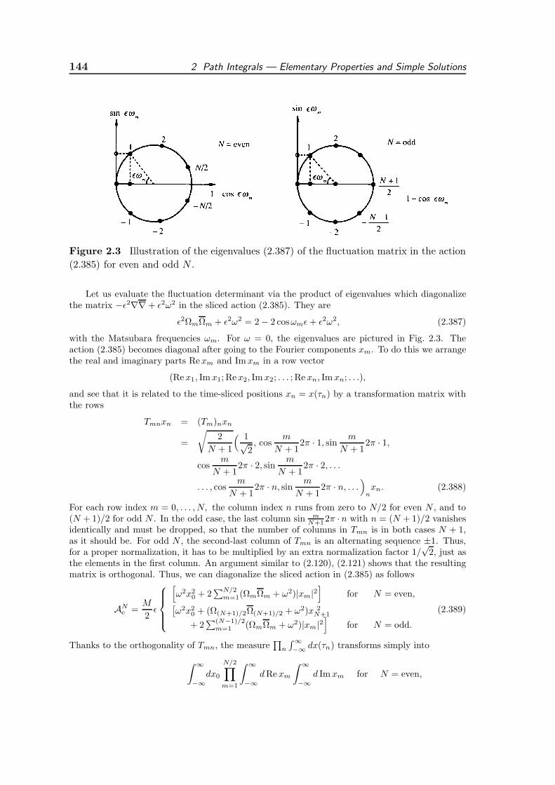
144 2 Path Integrals — Elementary Properties and Simple Solutions
Figure 2.3 Illustration of the eigenvalues (2.387) of the fluctuation matrix in the action
(2.385) for even and odd N .
Let us evaluate the fluctuation determinant via the product of eigenvalues which diagonalizethe matrix −ǫ2∇∇ + ǫ2ω2 in the sliced action (2.385). They are
ǫ2ΩmΩm + ǫ2ω2 = 2 − 2 cosωmǫ + ǫ2ω2, (2.387)
with the Matsubara frequencies ωm. For ω = 0, the eigenvalues are pictured in Fig. 2.3. Theaction (2.385) becomes diagonal after going to the Fourier components xm. To do this we arrangethe real and imaginary parts Rexm and Imxm in a row vector
(Rex1, Imx1; Rex2, Imx2; . . . ; Rexn, Imxn; . . .),
and see that it is related to the time-sliced positions xn = x(τn) by a transformation matrix withthe rows
Tmnxn = (Tm)nxn
=
√
2
N + 1
( 1√2, cos
m
N + 12π · 1, sin m
N + 12π · 1,
cosm
N + 12π · 2, sin m
N + 12π · 2, . . .
. . . , cosm
N + 12π · n, sin m
N + 12π · n, . . .
)
nxn. (2.388)
For each row index m = 0, . . . , N, the column index n runs from zero to N/2 for even N , and to(N + 1)/2 for odd N . In the odd case, the last column sin m
N+12π · n with n = (N + 1)/2 vanishesidentically and must be dropped, so that the number of columns in Tmn is in both cases N + 1,as it should be. For odd N , the second-last column of Tmn is an alternating sequence ±1. Thus,for a proper normalization, it has to be multiplied by an extra normalization factor 1/
√2, just as
the elements in the first column. An argument similar to (2.120), (2.121) shows that the resultingmatrix is orthogonal. Thus, we can diagonalize the sliced action in (2.385) as follows
ANe =
M
2ǫ
[
ω2x20 + 2
∑N/2m=1(ΩmΩm + ω2)|xm|2
]
for N = even,[
ω2x20 + (Ω(N+1)/2Ω(N+1)/2 + ω2)x 2
N+1
+ 2∑(N−1)/2
m=1 (ΩmΩm + ω2)|xm|2]
for N = odd.
(2.389)
Thanks to the orthogonality of Tmn, the measure∏
n
∫∞
−∞dx(τn) transforms simply into
∫ ∞
−∞
dx0
N/2∏
m=1
∫ ∞
−∞
dRexm
∫ ∞
−∞
d Imxm for N = even,
2.10 Quantum Statistics of the Harmonic Oscillator 145
(2.390)
∫ ∞
−∞
dx0
∫ ∞
−∞
dx(N+1)/2
(N−1)/2∏
m=1
∫ ∞
−∞
dRexm
∫ ∞
−∞
d Imxm for N = odd.
By performing the Gaussian integrals we obtain the partition function
ZNω =
[
detN+1(−ǫ2∇∇ + ǫ2ω2)]−1/2
=
[
N∏
m=0
(ǫ2ΩmΩm + ǫ2ω2)
]−1/2
=
N∏
m=0
[
2(1 − cosωmǫ) + ǫ2ω2]
−1/2
=
[
N∏
m=0
(
4 sin2 ωmǫ
2+ ǫ2ω2
)
]−1/2
. (2.391)
Thanks to the periodicity of the eigenvalues under the replacement n → n+N + 1, the result hasbecome a unique product expression for both even and odd N .
It is important to realize that contrary to the fluctuation factor (2.162) in the real-time am-plitude, the partition function (2.391) contains the square root of only positive eigenmodes as aunique result of Gaussian integrations. There are no phase subtleties as in the Fresnel integral(1.337).
To calculate the product, we observe that upon decomposing
sin2 ωmǫ
2=(
1 + cosωmǫ
2
)(
1 − cosωmǫ
2
)
, (2.392)
the sequence of first factors
1 + cosωmǫ
2≡ 1 + cos
πm
N + 1(2.393)
runs for m = 1, . . .N through the same values as the sequence of second factors
1 − cosωmǫ
2= 1 − cos
πm
N + 1≡ 1 + cosπ
N + 1 −m
N + 1, (2.394)
except in an opposite order. Thus, separating out the m = 0 -term, we rewrite (2.391) in the form
ZNω =
1
ǫω
[
N∏
m=1
2(
1 − cosωmǫ
2
)
]−1 [ N∏
m=1
(
1 +ǫ2ω2
4 sin2 ωmǫ2
)]−1/2
. (2.395)
The first factor on the right-hand side is the quantum-mechanical fluctuation determinant of thefree-particle determinant detN (−ǫ2∇∇) = N +1 [see (2.128)], so that we obtain for both even andodd N
ZNω =
kBT
hω
[
N∏
m=1
(
1 +ǫ2ω2
4 sin2 ωmǫ2
)]−1/2
. (2.396)
To evaluate the remaining product, we must distinguish again between even and odd cases of N .For even N , where every eigenvalue occurs twice (see Fig. 2.3), we obtain
ZNω =
kBT
hω
N/2∏
m=1
(
1 +ǫ2ω2
4 sin2 mπN+1
)
−1
. (2.397)
For odd N , the term with m = (N + 1)/2 occurs only once and must be treated separately so that
ZNω =
kBT
hω
(
1 +ǫ2ω2
4
)1/2 (N−1)/2∏
m=1
(
1 +ǫ2ω2
4 sin2 πmN+1
)
−1
. (2.398)
146 2 Path Integrals — Elementary Properties and Simple Solutions
We now introduce the parameter ωe, the Euclidean analog of (2.163), via the equations
sin iωeǫ
2≡ i
ωǫ
2, sinh
ωeǫ
2≡ ωǫ
2. (2.399)
In the odd case, the product formula17
(N−1)/2∏
m=1
[
1 − sin2 x
sin2 mπ(N+1)
]
=2
sin 2x
sin[(N + 1)x]
(N + 1)(2.400)
[similar to (2.165)] yields, with x = ωeǫ/2,
ZNω =
kBT
hω
[
1
sinh(ωeǫ/2)
sinh[(N + 1)ωeǫ/2]
N + 1
]−1
. (2.401)
In the even case, the formula18
N/2∏
m=1
[
1 − sin2 x
sin2 mπ(N+1)
]
=1
sinx
sin[(N + 1)x]
(N + 1), (2.402)
produces once more the same result as in Eq. (2.401). Inserting Eq. (2.399) leads to the partitionfunction on the sliced imaginary time axis:
ZNω =
1
2 sinh(hωeβ/2). (2.403)
The partition function can be expanded into the following series
ZNω = e−hωe/2kBT + e−3hωe/2kBT + e−5hωe/2kBT + . . . . (2.404)
By comparison with the general spectral expansion (2.328), we display the energy eigenvalues ofthe system:
En =
(
n +1
2
)
hωe. (2.405)
They show the typical linearly rising oscillator sequence with
ωe =2
ǫarsinh
ωǫ
2(2.406)
playing the role of the frequency on the sliced time axis, and hωe/2 being the zero-point energy.In the continuum limit ǫ → 0, the time-sliced partition function ZN
ω goes over into the usualoscillator partition function
Zω =1
2 sinh(βhω/2). (2.407)
In D dimensions this becomes, of course, [2 sinh(βhω/2)]−D, due to the additivity of the action ineach component of x.
Note that the continuum limit of the product in (2.396) can also be taken factor by factor.Then Zω becomes
Zω =kBT
hω
[
∞∏
m=1
(
1 +ω2
ω2m
)
]−1
. (2.408)
17I.S. Gradshteyn and I.M. Ryzhik, op. cit., Formula 1.391.1.18ibid., formula 1.391.3.
2.10 Quantum Statistics of the Harmonic Oscillator 147
According to formula (2.173), the product∏∞
m=1
(
1 + x2
m2π2
)
converges rapidly against sinhx/x
and we find with x = hωβ/2
Zω =kBT
hω
hω/2kBT
sinh(hω/2kBT )=
1
2 sinh(βhω/2). (2.409)
As discussed after Eq. (2.183), the continuum limit can be taken in each factor since the productin (2.396) contains only ratios of frequencies.
Just as in the quantum-mechanical case, this procedure of obtaining the continuum limit canbe summarized in the sequence of equations arriving at a ratio of differential operators
ZNω =
[
detN+1(−ǫ2∇∇ + ǫ2ω2)]−1/2
=[
det′N+1(−ǫ2∇∇)]−1/2
[
detN+1(−ǫ2∇∇ + ǫ2ω2)
det′N+1(−ǫ2∇∇)
]−1/2
ǫ→0−−−→ kBT
h
[
det(−∂2τ + ω2)
det′(−∂2τ )
]−1/2
=kBT
hω
∞∏
m=1
[
ω2m + ω2
ω2m
]−1
. (2.410)
In the ω = 0 -determinants, the zero Matsubara frequency is excluded to obtain a finite expression.This is indicated by a prime. The differential operator −∂2
τ acts on real functions which are periodicunder the replacement τ → τ+hβ. Remember that each eigenvalue ω2
m of −∂2τ occurs twice, except
for the zero frequency ω0 = 0, which appears only once.Let us finally mention that the results of this section could also have been obtained directly
from the quantum-mechanical amplitude (2.175) [or with the discrete times from (2.199)] by ananalytic continuation of the time difference tb − ta to imaginary values −i(τb − τa):
(xbτb|xaτa) =1
√
2πh/M
√
ω
sinhω(τb − τa)
× exp
− 1
2h
Mω
sinhω(τb − τa)[(x2
b + x2a) coshω(τb − τa) − 2xbxa]
. (2.411)
By setting x = xb = xa and integrating over x, we obtain [compare (2.333)]
Zω =
∫ ∞
−∞
dx (x τb|x τa) =1
√
2πh(τb − τa)/M
√
ω(τb − τa)
sinh[ω(τb − τa)]
×√
2πh sinh[ω(τb − τa)]/ωM
2 sinh[ω(τb − τa)/2]=
1
2 sinh[ω(τb − τa)/2]. (2.412)
Upon equating τb − τa = hβ, we retrieve the partition function (2.407). A similar treatment ofthe discrete-time version (2.199) would have led to (2.403). The main reason for presenting anindependent direct evaluation in the space of real periodic functions was to display the frequencystructure of periodic paths and to see the difference with respect to the quantum-mechanical pathswith fixed ends. We also wanted to show how to handle the ensuing product expressions.
For applications in polymer physics (see Chapter 15) one also needs the partition function ofall path fluctuations with open ends
Zopenω =
∫ ∞
−∞
dxb
∫ ∞
−∞
dxa (xbτb|xaτa) =1
√
2πh(τb − τa)/M
√
ω(τb − τa)
sinh[ω(τb − τa)]
2πh
Mω
=
√
2πh
Mω
1√
sinh[ω(τb − τa)]. (2.413)
The prefactor is√
2π times the length scale λω of Eq. (2.303).
148 2 Path Integrals — Elementary Properties and Simple Solutions
2.11 Time-Dependent Harmonic Potential
It is often necessary to calculate thermal fluctuation determinants for the case of a time-dependentfrequency Ω(τ) which is periodic under τ → τ + hβ. As in Section 2.3.6, we consider the amplitude
(xbτb|xaτa) =
∫
D′x
∫ Dp
2πhe−∫
τb
τadτ [−ipx+p2/2M+MΩ2(τ)x2/2]/h
=
∫
Dxe−∫
τb
τadτ [Mx2+Ω2(τ)x2]/2h
. (2.414)
The time-sliced fluctuation factor is [compare (2.202)]
FN (τa − τb) = detN+1[−ǫ2∇∇ + ǫΩ2(τ)]−1/2, (2.415)
with the continuum limit
F (τa − τb) =kBT
h
[
det(−∂2τ + Ω2(τ))
det′(−∂2τ )
]−1/2
. (2.416)
Actually, in the thermal case it is preferable to use the oscillator result for normalizing thefluctuation factor, rather than the free-particle result, and to work with the formula
F (τb, τa) =1
2 sinh(βhω/2)
[
det(−∂2τ + Ω2(τ))
det(−∂2τ + ω2)
]−1/2
. (2.417)
This has the advantage that the determinant in the denominator contains no zero eigenvalue whichwould require a special treatment as in (2.410); the operator −∂2
τ + ω2 is positive.As in the quantum-mechanical case, the spectrum of eigenvalues is not known for general Ω(τ).
It is, however, possible to find a differential equation for the entire determinant, analogous to theGelfand-Yaglom formula (2.209), with the initial condition (2.214), although the derivation is nowmuch more tedious. The origin of the additional difficulties lies in the periodic boundary conditionwhich introduces additional nonvanishing elements −1 in the upper right and lower left corners ofthe matrix −ǫ2∇∇ [compare (2.107)]:
−ǫ2∇∇ =
2 −1 0 . . . 0 0 −1−1 2 −1 . . . 0 0 0...
...0 0 0 . . . −1 2 −1−1 0 0 . . . 0 −1 2
. (2.418)
To better understand the relation with the previous result we shall replace the corner elements−1 by −α which can be set equal to zero at the end, for a comparison. Adding to −ǫ2∇∇ atime-dependent frequency matrix we then consider the fluctuation matrix
−ǫ2∇∇ + ǫ2Ω2 =
2 + ǫ2Ω2N+1 −1 0 . . . 0 −α
−1 2 + ǫ2Ω2N −1 . . . 0 0
......
−α 0 0 . . . −1 2 + ǫ2Ω21
.
(2.419)
Let us denote the determinant of this (N + 1)× (N + 1) matrix by DN+1. Expanding it along thefirst column, it is found to satisfy the equation
DN+1 = (2 + ǫ2Ω2N+1) (2.420)
×detN
2 + ǫ2Ω2N −1 0 . . . 0 0
......
0 0 0 . . . −1 2 + ǫ2Ω21
2.11 Time-Dependent Harmonic Potential 149
+detN
−1 0 0 0 . . . 0 −α−1 2 + ǫ2Ω2
N−1 −1 0 . . . 0 00 −1 2 + ǫ2Ω2
N−2 −1 . . . 0 0...
...0 0 0 0 . . . −1 2 + ǫ2Ω2
1
+(−1)N+1αdetN
−1 0 0 . . . 0 −α2 + ǫ2Ω2
N −1 0 . . . 0 0−1 2 + ǫ2Ω2
N−1 −1 . . . 0 0...
...0 0 0 . . . 2 + ǫ2Ω2
2 −1
.
The first determinant was encountered before in Eq. (2.204) (except that there it appeared with−ǫ2Ω2 instead of ǫ2Ω2). There it was denoted by DN , satisfying the difference equation
(
−ǫ2∇∇ + ǫ2Ω2N+1
)
DN = 0, (2.421)
with the initial conditions
D1 = 2 + ǫ2Ω21,
D2 = (2 + ǫ2Ω21)(2 + ǫ2Ω2
2) − 1. (2.422)
The second determinant in (2.420) can be expanded with respect to its first column yielding
−DN−1 − α. (2.423)
The third determinant is more involved. When expanded along the first column it gives
(−1)N[
1 + (2 + ǫ2Ω2N )HN−1 −HN−2
]
, (2.424)
with the (N − 1) × (N − 1) determinant
HN−1 ≡ (−1)N−1 (2.425)
×detN−1
0 0 0 . . . 0 0 −α2 + ǫ2Ω2
N−1 −1 0 . . . 0 0 0−1 2 + ǫ2Ω2
N−2 −1 . . . 0 0 0...
...0 0 0 . . . −1 2 + ǫ2Ω2
2 −1
.
By expanding this along the first column, we find that HN satisfies the same difference equationas DN :
(−ǫ2∇∇ + ǫ2Ω2N+1)HN = 0. (2.426)
However, the initial conditions for HN are different:
H2 =
∣
∣
∣
∣
0 −α2 + ǫ2Ω2
2 −1
∣
∣
∣
∣
= α(2 + ǫ2Ω22), (2.427)
H3 = −
∣
∣
∣
∣
∣
∣
∣
∣
0 0 −α2 + ǫ2Ω2
3 −1 0−1 2 + ǫ2Ω2
2 −1
∣
∣
∣
∣
∣
∣
∣
∣
= α[
(2 + ǫ2Ω22)(2 + ǫ2Ω2
3) − 1]
. (2.428)
150 2 Path Integrals — Elementary Properties and Simple Solutions
They show that HN is in fact equal to αDN−1, provided we shift Ω2N by one lattice unit upwards
to Ω2N+1. Let us indicate this by a superscript +, i.e., we write
HN = αD+N−1. (2.429)
Thus we arrive at the equation
DN+1 = (2 + ǫ2Ω2N )DN −DN−1 − α
−α[1 + (2 + ǫ2Ω2N )αD+
N−2 − αD+N−3]. (2.430)
Using the difference equations for DN and D+N , this can be brought to the convenient form
DN+1 = DN+1 − α2D+N−1 − 2α. (2.431)
For quantum-mechanical fluctuations with α = 0, this reduces to the earlier result in Section 2.3.6.For periodic fluctuations with α = 1, the result is
DN+1 = DN+1 −D+N−1 − 2. (2.432)
In the continuum limit, DN+1 − D+N−1 tends towards 2Dren, where Dren(τ) = Da(t) is the
imaginary-time version of the Gelfand-Yaglom function in Section 2.4 solving the homogenousdifferential equation (2.215), with the initial conditions (2.213) and (2.214), or Eqs. (2.228). Thecorresponding properties are now:
[
−∂2τ + Ω2(τ)
]
Dren(τ) = 0, Dren(0) = 0, Dren(0) = 1. (2.433)
In terms of Dren(τ), the determinant is given by the Gelfand-Yaglom-like formula
det(−ǫ2∇∇ + ǫΩ2)Tǫ→0−−−→ 2[Dren(hβ) − 1], (2.434)
and the partition function reads
ZΩ =1
√
2[
Dren(hβ) − 1]
. (2.435)
The result may be checked by going back to the amplitude (xbtb|xata) of Eq. (2.262), continuingit to imaginary times t = iτ , setting xb = xa = x, and integrating over all x. The result is
ZΩ =1
2√
Da(tb) − 1, tb = ihβ, (2.436)
in agreement with (2.435).As an example, take the harmonic oscillator for which the solution of (2.433) is
Dren(τ) =1
ωsinhωτ (2.437)
[the analytically continued (2.216)]. Then
2[Dren(τ) − 1] = 2(coshβhω − 1) = 4 sinh2(βhω/2), (2.438)
and we find the correct partition function:
Zω =
2[Dren(τ) − 1]−1/2 ∣
∣
∣
τ=hβ
=1
2 sinh(βhω/2). (2.439)
2.12 Functional Measure in Fourier Space 151
On a sliced imaginary-time axis, the case of a constant frequency Ω2 ≡ ω2 is solved as follows.From Eq. (2.210) we take the ordinary Gelfand-Yaglom function DN , and continue it to Euclideanωe, yielding the imaginary-time version
DN =sinh(N + 1)ωeǫ
sinh ωeǫ. (2.440)
Then we use formula (2.432), which simplifies for a constant Ω2 ≡ ω2 for which D+N−1 = DN−1,
and calculate
DN+1 =1
sinh ωeǫ[sinh(N + 2)ωeǫ− sinhNωeǫ] − 2
= 2 [cosh(N + 1)ωeǫ− 1] = 4 sinh2[(N + 1)ωeǫ/2]. (2.441)
Inserting this into Eq. (2.386) yields the partition function
Zω =1
√
DN+1
=1
2 sinh(hωeβ/2), (2.442)
in agreement with (2.403).
2.12 Functional Measure in Fourier Space
There exists an alternative definition for the quantum-statistical path integral whichis useful for some applications (for example in Section 2.13 and in Chapter 5). Thelimiting product formula (2.410) suggests that instead of summing over all zigzagconfigurations of paths on a sliced time axis, a path integral may be defined withthe help of the Fourier components of the paths on a continuous time axis. As in(2.380), but with a slightly different normalization of the coefficients, we expandthese paths here as
x(τ) = x0 + η(τ) ≡ x0 +∞∑
m=1
(
xmeiωmτ + c.c.
)
, x0 = real, x−m ≡ x∗m. (2.443)
Note that the temporal integral over the time-dependent fluctuations η(τ) is zero,∫ h/kBT0 dτ η(τ) = 0, so that the zero-frequency component x0 is the temporal averageof the fluctuating paths:
x0 = x ≡ kBT
h
∫ h/kBT
0dτ x(τ). (2.444)
In contrast to (2.380) which was valid on a sliced time axis and was thereforesubject to a restriction on the range of the m-sum, the present sum is unrestrictedand runs over all Matsubara frequencies ωm = 2πmkBT/h = 2πm/hβ. In terms ofxm, the Euclidean action of the linear oscillator is
Ae =M
2
∫ h/kBT
0dτ (x2 + ω2x2)
=Mh
kBT
[
ω2
2x20 +
∞∑
m=1
(ω2m + ω2)|xm|2
]
. (2.445)
152 2 Path Integrals — Elementary Properties and Simple Solutions
The integration variables of the time-sliced path integral were transformed to theFourier components xm in Eq. (2.388). The product of integrals
∏
n
∫∞−∞ dx(τn)
turned into the product (2.390) of integrals over real and imaginary parts of xm. Inthe continuum limit, the result is
∫ ∞
−∞dx0
∞∏
m=1
∫ ∞
−∞dRexm
∫ ∞
−∞d Im xm. (2.446)
Placing the exponential e−Ae/h with the frequency sum (2.445) into the integrand,the product of Gaussian integrals renders a product of inverse eigenvalues (ω2
m+ω2)−1
for m = 1, . . . ,∞, with some infinite factor. This may be determined by comparisonwith the known continuous result (2.410) for the harmonic partition function. Theinfinity is of the type encountered in Eq. (2.183), and must be divided out of themeasure (2.446). The correct result (2.408) is obtained from the following measureof integration in Fourier space
∮
Dx ≡∫ ∞
−∞
dx0le(hβ)
∞∏
m=1
[
∫ ∞
−∞
∫ ∞
−∞
dRexmd ImxmπkBT/Mω2
m
]
. (2.447)
The divergences in the product over the factors (ω2m + ω2)−1 discussed after
Eq. (2.183) are canceled by the factors ω2m in the measure. It will be convenient to
introduce a short-hand notation for the measure on the right-hand side, writing itas
∮
Dx ≡∫ ∞
−∞
dx0le(hβ)
∮
D′x. (2.448)
The denominator of the x0-integral is the length scale le(hβ) associated with βdefined in Eq. (2.353).
Then we calculate
Zx0ω ≡
∮
D′x e−Ae/h =∞∏
m=1
[
∫ ∞
−∞
∫ ∞
−∞
dRexmd Im xmπkBT/Mω2
m
]
e−Mh[ω2x20/2+
∑
∞
m=1(ω2
m+ω2)|xm|2]/kBT
= e−Mω2x20/2kBT
∞∏
m=1
[
ω2m + ω2
ω2m
]−1
. (2.449)
The final integral over the zero-frequency component x0 yields the partition function
Zω =∮
Dx e−Ae/h =∫ ∞
−∞
dx0le(hβ)
Zx0ω =
kBT
hω
∞∏
m=1
[
ω2m + ω2
ω2m
]−1
, (2.450)
as in (2.410).The same measure can be used for the more general amplitude (2.414), as is
obvious from (2.416). With the predominance of the kinetic term in the measureof path integrals [the divergencies discussed after (2.183) stem only from it], it can
2.12 Functional Measure in Fourier Space 153
easily be shown that the same measure is applicable to any system with the standardkinetic term.
It is also possible to find a Fourier decomposition of the paths and an associatedintegration measure for the open-end partition function in Eq. (2.413). We begin byconsidering the slightly reduced set of all paths satisfying the Neumann boundaryconditions
x(τa) = va = 0, x(τb) = vb = 0. (2.451)
They have the Fourier expansion
x(τ) = x0 + η(τ) = x0 +∞∑
n=1
xn cos νn(τ − τa), νn = nπ/β. (2.452)
The frequencies νn are the Euclidean version of the frequencies (3.64) for Dirichletboundary conditions. Let us calculate the partition function for such paths byanalogy with the above periodic case by a Fourier decomposition of the action
Ae =M
2
∫ h/kBT
0dτ (x2 + ω2x2) =
Mh
kBT
[
ω2
2x20 +
1
2
∞∑
n=1
(ν2n + ω2)x2n
]
, (2.453)
and of the measure
∮
Dx ≡∫ ∞
−∞
dx0le(hβ)
∞∏
n=1
[
∫ ∞
−∞
∫ ∞
−∞
d xnπkBT/2Mν2n
]
≡∫ ∞
−∞
dx0le(hβ)
∮
D′x. (2.454)
We now perform the path integral over all fluctuations at fixed x0 as in (2.449):
ZN,x0ω ≡
∮
D′x e−Ae/h =∞∏
n=1
[
∫ ∞
−∞
∫ ∞
−∞
d xnπkBT/2Mν2n
]
e−Mh[ω2x20/2+
∑
∞
n=1(ν2n+ω2)|xn|2]/kBT
= e−Mω2x20/2kBT
∞∏
n=1
[
ν2n + ω2
ν2n
]−1
. (2.455)
Using the product formula (2.183), this becomes
ZN,x0ω =
√
ωhβ
sinhωhβexp
(
−βM2ω2x20
)
. (2.456)
The final integral over the zero-frequency component x0 yields the partition function
ZNω =
1
le(hβ)
√
2πh
Mω
1√sinhωhβ
. (2.457)
We have replaced the denominator in the prefactor 1/le(hβ) by the length scale1/le(hβ) of Eq. (2.353). Apart from this prefactor, the Neumann partition functioncoincides precisely with the open-end partition function Zopen
ω in Eq. (2.413).
154 2 Path Integrals — Elementary Properties and Simple Solutions
What is the reason for this coincidence up to a trivial factor, even though thepaths satisfying Neumann boundary conditions do not comprise all paths with openends? Moreover, the integrals over the endpoints in the defining equation (2.413) donot force the endpoint velocities , but rather endpoint momenta to vanish. Indeed,recalling Eq. (2.189) for the time evolution amplitude in momentum space we cansee immediately that the partition function with open ends Zopen
ω in Eq. (2.413) isidentical to the imaginary-time amplitude with vanishing endpoint momenta:
Zopenω = (pb hβ|pa 0)|pb=pa=0. (2.458)
Thus, the sum over all paths with arbitrary open ends is equal to the sum of allpaths satisfying Dirichlet boundary conditions in momentum space. Only classically,the vanishing of the endpoint momenta implies the vanishing of the endpoint veloc-ities. From the general discussion of the time-sliced path integral in phase space inSection 2.1 we know that fluctuating paths have Mx 6= p. The fluctuations of thedifference are controlled by a Gaussian exponential of the type (2.53). This leads tothe explanation of the trivial factor between Zopen
ω and ZNω . The difference between
Mx and p appears only in the last short-time intervals at the ends. But at shorttime, the potential does not influence the fluctuations in (2.53). This is the reasonwhy the fluctuations at the endpoints contribute only a trivial overall factor le(hβ)to the partition function ZN
ω .
2.13 Classical Limit
The alternative measure of the last section serves to show, somewhat more convinc-ingly than before, that in the high-temperature limit the path integral representationof any quantum-statistical partition function reduces to the classical partition func-tion as stated in Eq. (2.346). We start out with the Lagrangian formulation (2.376).Inserting the Fourier decomposition (2.443), the kinetic term becomes
∫ hβ
0dτ
M
2x2 =
Mh
kBT
∞∑
m=1
ω2m|xm|2, (2.459)
and the partition function reads
Z =∮
Dx exp
[
− M
kBT
∞∑
m=1
ω2m|xm|2 −
1
h
∫ h/kBT
0dτ V (x0 +
∞∑
m=−∞
′ xme−iωmτ )
]
. (2.460)
The summation symbol with a prime implies the absence of the m = 0 -term. Themeasure is the product (2.447) of integrals of all Fourier components.
We now observe that for large temperatures, the Matsubara frequencies form 6= 0diverge like 2πmkBT/h . This has the consequence that the Boltzmann factor forthe xm6=0 fluctuations becomes sharply peaked around xm = 0. The average size of
xm is√
kBT/M/ωm = h/2πm√MkBT . If the potential V
(
x0 +∑′ ∞
m=−∞′ xme
−iωmτ)
is a smooth function of its arguments, we can approximate it by V (x0) plus terms

2.14 Calculation Techniques on Sliced Time Axis via the Poisson Formula 155
containing higher powers of xm. For large temperatures, these are small on theaverage and can be ignored. The leading term V (x0) is time-independent. Hencewe obtain in the high-temperature limit
ZT→∞−−−→
∮
Dx exp[
− M
kBT
∞∑
m=1
ω2m|xm|2 −
1
kBTV (x0)
]
. (2.461)
The right-hand side is quadratic in the Fourier components xm. With the measureof integration (2.447), we perform the integrals over xm and obtain
ZT→∞−−−→ Zcl =
∫ ∞
−∞
dx0le(hβ)
e−V (x0)/kBT . (2.462)
This agrees with the classical statistical partition function (2.352).The derivation reveals an important prerequisite for the validity of the classical
limit: It holds only for sufficiently smooth potentials. We shall see in Chapter 8that for singular potentials such as −1/|x| (Coulomb), 1/|x|2 (centrifugal barrier),1/ sin2 θ (angular barrier), this condition is not fulfilled and the classical limit is nolonger given by (2.462). The particle distribution ρ(x) at a fixed x does not havethis problem. It always tends towards the naively expected classical limit (2.354):
ρ(x)T→∞−−−→ Z−1
cl e−V (x)/kBT . (2.463)
The convergence is nonuniform in x, which is the reason why the limit does notalways carry over to the integral (2.462). This will be an important point in derivingin Chapter 12 a new path integral formula valid for singular potentials. At first, weshall ignore such subtleties and continue with the conventional discussion valid forsmooth potentials.
2.14 Calculation Techniques on Sliced Time Axis
via the Poisson Formula
In the previous sections we have used tabulated product formulas such as (2.127), (2.165), (2.173),(2.400), (2.402) to find fluctuation determinants on a finite sliced time axis. With the recentinterest in lattice models of quantum field theories, it is useful to possess an efficient calculationaltechnique to derive such product formulas (and related sums). Consider, as a typical example, thequantum-statistical partition function for a harmonic oscillator of frequency ω on a time axis withN + 1 slices of thickness ǫ,
Z =
N∏
m=0
[2(1 − cosωmǫ) + ǫ2ω2]−1/2, (2.464)
with the product running over all Matsubara frequencies ωm = 2πmkBT/h. Instead of dealingwith this product it is advantageous to consider the free energy
F = −kBT logZ =1
2kBT
N∑
m=0
log[2(1 − cosωmǫ) + ǫ2ω2]. (2.465)
156 2 Path Integrals — Elementary Properties and Simple Solutions
We now observe that by virtue of Poisson’s summation formula (1.205), the sum can be rewrittenas the following combination of a sum and an integral:
F =1
2kBT (N + 1)
∞∑
n=−∞
∫ 2π
0
dλ
2πeiλn(N+1) log[2(1 − cosλ) + ǫ2ω2]. (2.466)
The sum over n squeezes λ to integer multiples of 2π/(N + 1) = ωmǫ which is precisely what wewant.
We now calculate the integrals in (2.466):
∫ 2π
0
dλ
2πeiλn(N+1) log[2(1 − cosλ) + ǫ2ω2]. (2.467)
For this we rewrite the logarithm of an arbitrary positive argument as the limit
log a = limδ→0
[
−∫ ∞
δ
dτ
τe−τa/2
]
+ log(2δ) + γ, (2.468)
where
γ ≡ −Γ′(1)/Γ(1) = limN→∞
(
N∑
n=1
1
n− logN
)
≈ 0.5773156649 . . . (2.469)
is the Euler-Mascheroni constant. Indeed, the function
E1(x) =
∫ ∞
x
dt
te−t (2.470)
is known as the exponential integral with the small-x expansion19
E1(x) = −γ − log x−∞∑
k=1
(−x)k
kk!. (2.471)
With the representation (2.468) for the logarithm, the free energy can be rewritten as
F =1
2ǫ
∞∑
n=−∞
limδ→0
−∫ ∞
δ
dτ
τ
∫ 2π
0
dλ
2πeiλn(N+1)−τ [2(1−cosλ)+ǫ2ω2]/2 − δn0 [log(2δ) + γ]
.
(2.472)
The integral over λ is now performed20 giving rise to a modified Bessel function In(N+1)(τ):
F =1
2ǫ
∞∑
n=−∞
limδ→0
−∫ ∞
δ
dτ
τIn(N+1)(τ)e−τ(2+ǫ2ω2)/2 − δn0 [log(2δ) + γ]
.
(2.473)
If we differentiate this with respect to ǫ2ω2 ≡ m2, we obtain
∂F
∂m2=
1
4ǫ
∞∑
n=−∞
∫ ∞
0
dτIn(N+1)(τ)e−τ(2+m2)/2 (2.474)
and perform the τ -integral, using the formula valid for Re ν > −1, Re α > Re µ
∫ ∞
0
dτ Iν(µτ)e−τα = µν (α−√
α2 − µ2)−ν ,√
α2 − µ2= µ−ν (α−
√
α2 − µ2)ν√
α2 − µ2, (2.475)
19I.S. Gradshteyn and I.M. Ryzhik, op. cit., Formula 8.214.2.20I.S. Gradshteyn and I.M. Ryzhik, op. cit., Formulas 8.411.1 and 8.406.1.
2.14 Calculation Techniques on Sliced Time Axis via the Poisson Formula 157
to find
∂F
∂m2=
1
2ǫ
∞∑
n=−∞
1√
(m2 + 2)2 − 4
[
m2 + 2 −√
(m2 + 2)2 − 4
2
]|n|(N+1)
. (2.476)
From this we obtain F by integration over m2 + 1. The n = 0 -term under the sum gives
log[(m2 + 2 +√
(m2 + 2)2 − 4 )/2] + const (2.477)
and the n 6= 0 -terms:
− 1
|n|(N + 1)[(m2 + 2 +
√
(m2 + 2)2 − 4 )/2]−|n|(N+1) + const , (2.478)
where the constants of integration can depend on n(N + 1). They are adjusted by going to thelimit m2 → ∞ in (2.473). There the integral is dominated by the small-τ regime of the Besselfunctions
Iα(z) ∼ 1
|α|!(z
2
)α
[1 + O(z2)], (2.479)
and the first term in (2.473) becomes
− 1
(|n|(N + 1))!
∫ ∞
δ
dτ
τ
(τ
2
)|n|(N+1)
e−τm2/2
≈
logm2 + γ + log(2δ) n = 0
−(m2)−|n|(N+1)/|n|(N + 1) n 6= 0
. (2.480)
The limit m2 → ∞ in (2.477), (2.478) gives, on the other hand, logm2 + const and−(m2)−|n|(N+1)/|n|(N + 1) + const , respectively. Hence the constants of integration must bezero. We can therefore write down the free energy for N + 1 time steps as
F =1
2β
N∑
m=0
log[2(1 − cos(ωmǫ)) + ǫ2ω2]
=1
2ǫ
log[(
ǫ2ω2 + 2 +√
(ǫ2ω2 + 2)2 − 4)
/
2]
(2.481)
− 2
N + 1
∞∑
n=1
1
n
[(
ǫ2ω2 + 2 +√
(ǫ2ω2 + 2)2 − 4)
/
2]−|n|(N+1)
.
Here it is convenient to introduce the parameter
ǫωe ≡ log[
ǫ2ω2 + 2 +√
(ǫ2ω2 + 2)2 − 4]
/
2
, (2.482)
which satisfies
cosh(ǫωe) = (ǫ2ω2 + 2)/2, sinh(ǫωe) =√
(ǫ2ω2 + 2)2 − 4/2, (2.483)
or
sinh(ǫωe/2) = ǫω/2.
Thus it coincides with the parameter introduced in (2.399), which brings the free energy (2.481)to the simple form
F =h
2
[
ωe −2
ǫ(N + 1)
∞∑
n=1
1
ne−ǫωen(N+1)
]
=1
2
[
hωe + 2kBT log(1 − e−βhωe)]
=1
βlog [2 sinh(βhωe/2)] , (2.484)
158 2 Path Integrals — Elementary Properties and Simple Solutions
whose continuum limit is
Fǫ→0=
1
βlog [2 sinh (βhω/2)] =
hω
2+
1
βlog(1 − e−βhω). (2.485)
2.15 Field-Theoretic Definition of Harmonic Path Integrals
by Analytic Regularization
A slight modification of the calculational techniques developed in the last sectionfor the quantum partition function of a harmonic oscillator can be used to definethe harmonic path integral in a way which neither requires time slicing, as in theoriginal Feynman expression (2.66), nor a precise specification of the integrationmeasure in terms of Fourier components, as in Section 2.12. The path integral forthe partition function
Zω =∮
Dxe−∫ hβ
0M [x2(τ)+ω2x2(τ)]/2 =
∮
Dxe−∫ hβ
0Mx(τ)[−∂2
τ+ω2]x(τ)/2 (2.486)
is formally evaluated as
Zω =1
√
Det(−∂2τ + ω2)= e−
12Tr log(−∂2
τ+ω2). (2.487)
Since the determinant of an operator is the product of all its eigenvalues, we maywrite, again formally,
Zω =∏
ω′
1√ω′2 + ω2
. (2.488)
The product runs over an infinite set of quantities which grow with ω′2, thus beingcertainly divergent. It may be turned into a divergent sum by rewriting Zω as
Zω ≡ e−Fω/kBT = e−12
∑
ω′log(ω′2+ω2). (2.489)
This expression has two unsatisfactory features. First, it requires a proper definitionof the formal sum over a continuous set of frequencies. Second, the logarithm ofthe dimensionful arguments ω2
m + ω2 must be turned into a meaningful expression.The latter problem would be removed if we were able to exchange the logarithmby log[(ω′2 + ω2)/ω2]. This would require the formal sum
∑
ω′ log ω2 to vanish. Weshall see below in Eq. (2.514) that this is indeed one of the pleasant properties ofanalytic regularization.
At finite temperatures, the periodic boundary conditions along the imaginary-time axis make the frequencies ω′ in the spectrum of the differential operator−∂2τ+ω2
discrete, and the sum in the exponent of (2.489) becomes a sum over all Matsubarafrequencies ωm = 2πkBT/h (m = 0,±1,±2, . . .):
Zω = exp
[
−1
2
∞∑
m=−∞
log(ω2m + ω2)
]
. (2.490)
2.15 Field-Theoretic Definition of Harmonic Path Integrals by Analytic Regularization 159
For the free energy Fω ≡ (1/β) logZω, this implies
Fω =1
2βTr log(−∂2τ + ω2)
∣
∣
∣
per=
1
2β
∞∑
m=−∞
log(ω2m + ω2). (2.491)
where the subscript per emphasizes the periodic boundary conditions in the τ -interval (0, hβ).
2.15.1 Zero-Temperature Evaluation of the Frequency Sum
In the limit T → 0, the sum in (2.491) goes over into an integral, and the free energybecomes
Fω ≡ 1
2βTr log(−∂2τ + ω2)
∣
∣
∣
±∞=h
2
∫ ∞
−∞
dω′
2πlog(ω′2 + ω2), (2.492)
where the subscript ±∞ indicates the vanishing boundary conditions of the eigen-functions at τ = ±∞. Thus, at low temperature, we can replace the frequency sumin the exponent of (2.489) by
∑
ω′
−−−→T→0
hβ∫ ∞
−∞
dω′
2π. (2.493)
This could have been expected on the basis of Planck’s rules for the phase spaceinvoked earlier on p. 97 to explain the measure of path integration. According tothese rules, the volume element in the phase space of energy and time has the mea-sure
∫
dt dE/h =∫
dt dω/2π. If the integrand is independent of time, the temporalintegral produces an overall factor , which for the imaginary-time interval (0, hβ) ofstatistical mechanics is equal to hβ = h/kBT , thus explaining the integral versionof the sum (2.493).
The integral on the right-hand side of (2.492) diverges at large ω′. This is calledan ultraviolet divergence (UV-divergence), alluding to the fact that the ultravioletregime of light waves contains the high frequencies of the spectrum.
The important observation is now that the divergent integral (2.492) can bemade finite by a mathematical technique called analytic regularization.21 This isbased on rewriting the logarithm log(ω′2 + ω2) in the derivative form:
log(ω′2 + ω2) = − d
dǫ(ω′2 + ω2)−ǫ
∣
∣
∣
∣
∣
ǫ=0
. (2.494)
Equivalently, we may obtain the logarithm from an ǫ → 0 -limit of the function
lMS(ǫ) = −1
ǫ(ω′2 + ω2)−ǫ +
1
ǫ. (2.495)
21G. ’t Hooft and M. Veltman, Nucl. Phys. B 44 , 189 (1972). Analytic regularization is atpresent the only method that allows to renormalize nonabelian gauge theories without destroyinggauge invariance. See also the review by G. Leibbrandt, Rev. Mod. Phys. 74 , 843 (1975).
160 2 Path Integrals — Elementary Properties and Simple Solutions
The subtraction of the pole term 1/ǫ is commonly referred to a minimal subtraction.Indicating this process by a subscript MS, we may write
lMS(ǫ) = −1
ǫ(ω′2 + ω2)−ǫ
∣
∣
∣
∣
MS, ǫ→0. (2.496)
Using the derivative formula (2.494), the trace of the logarithm in the free energy(2.492) takes the form
1
hβTr log(−∂2τ + ω2) = − d
dǫ
∫ ∞
−∞
dω′
2π(ω′2 + ω2)−ǫ
∣
∣
∣
∣
∣
ǫ=0
. (2.497)
We now set up a useful integral representation, due to Schwinger, for a power a−ǫ
generalizing (2.468). Using the defining integral representation for the Gamma func-tion
∫ ∞
0
dτ
ττµe−τω2
= ω−µ/2Γ(µ), (2.498)
the desired generalization is
a−ǫ =1
Γ(ǫ)
∫ ∞
0
dτ
ττ ǫe−τa. (2.499)
This allows us to re-express (2.497) as
1
hβTr log(−∂2τ + ω2) = − d
dǫ
1
Γ(ǫ)
∫ ∞
−∞
dω′
2π
∫ ∞
0
dτ
ττ ǫe−τ(ω′2+ω2)
∣
∣
∣
∣
∣
ǫ=0
. (2.500)
As long as ǫ is larger than zero, the τ -integral converges absolutely, so that we caninterchange the τ - and ω′-integrations, and obtain
1
hβTr log(−∂2τ + ω2) = − d
dǫ
1
Γ(ǫ)
∫ ∞
0
dτ
ττ ǫ∫ ∞
−∞
dω′
2πe−τ(ω′2+ω2)
∣
∣
∣
∣
∣
ǫ=0
. (2.501)
At this point we can perform the Gaussian integral over ω′ using formula (1.338),and find
1
hβTr log(−∂2τ + ω2) = − d
dǫ
1
Γ(ǫ)
∫ ∞
0
dτ
ττ ǫ
1
2√τπe−τω2
∣
∣
∣
∣
∣
ǫ=0
. (2.502)
For small ǫ, the τ -integral is divergent at the origin. It can, however, be defined byan analytic continuation of the integral starting from the regime ǫ > 1/2, where itconverges absolutely, to ǫ = 0. The continuation must avoid the pole at ǫ = 1/2.Fortunately, this continuation is trivial since the integral can be expressed in terms ofthe Gamma function, whose analytic properties are well-known. Using the integralformula (2.498), we obtain
1
hβTr log(−∂2τ + ω2) = − 1
2√πω1−2ǫ d
dǫ
1
Γ(ǫ)Γ(ǫ− 1/2)
∣
∣
∣
∣
∣
ǫ=0
. (2.503)
2.15 Field-Theoretic Definition of Harmonic Path Integrals by Analytic Regularization 161
The right-hand side has to be continued analytically from ǫ > 1/2 to ǫ = 0. This iseasily done using the defining property of the Gamma function Γ(x) = Γ(1 + x)/x,from which we find Γ(−1/2) = −2Γ(1/2) = −2
√π, and 1/Γ(ǫ) ≈ ǫ/Γ(1 + ǫ) ≈ ǫ.
The derivative with respect to ǫ leads to the free energy of the harmonic oscillatorat low temperature via analytic regularization:
1
hβTr log(−∂2τ + ω2) =
∫ ∞
−∞
dω′
2πlog(ω′2 + ω2) = ω, (2.504)
so that the free energy of the oscillator at zero-temperature becomes
Fω =hω
2. (2.505)
This agrees precisely with the result obtained from the lattice definition of the pathintegral in Eq. (2.407), or from the path integral (3.808) with the Fourier measure(2.447).
With the above procedure in mind, we shall often use the sloppy formula ex-pressing the derivative of Eq. (2.499) at ǫ = 0:
log a = −∫ ∞
0
dτ
τe−τa. (2.506)
This formula differs from the correct one by a minimal subtraction and can beused in all calculations with analytic regularization. Its applicability is based onthe possibility of dropping the frequency integral over 1/ǫ in the alternative correctexpression
1
hβTr log(−∂2τ + ω2) = −1
ǫ
∫ ∞
−∞
dω′
2π
[
1
ǫ(ω′2 + ω2)−ǫ − 1
ǫ
]
ǫ→0. (2.507)
In fact, within analytic regularization one may set all integrals over arbitrary purepowers of the frequency equal to zero:
∫ ∞
0dω′ (ω′)α = 0 for all α. (2.508)
This is known as Veltman’s rule.22 It is a special limit of a frequency integral whichis a generalization of the integral in (2.497):
∫ ∞
−∞
dω′
2π
(ω′2)γ
(ω′2 + ω2)ǫ=
Γ(γ + 1/2)
2πΓ(ǫ)(ω2)γ+1/2−ǫ. (2.509)
This equation may be derived by rewriting the left-hand side as
1
Γ(ǫ)
∫ ∞
−∞
dω′
2π(ω′2)γ
∫ ∞
0
dτ
ττ ǫe−τ(ω′2+ω2). (2.510)
22See the textbook H. Kleinert and V. Schulte-Frohlinde, Critical Properties of φ4-Theories ,World Scientific, Singapore, 2001 (http://www.physik.fu-berlin.de/~kleinert/b8).
162 2 Path Integrals — Elementary Properties and Simple Solutions
The integral over ω′ is performed as follows:
∫ ∞
−∞
dω′
2π(ω′2)γe−τ(ω′2+ω2) =
1
2π
∫ ∞
0
dω′ 2
ω′ 2(ω′2)γ+1/2e−τ(ω′2+ω2) =
τ−γ−1/2
2πΓ(γ + 1/2),
(2.511)leading to a τ -integral in (2.510)
∫ ∞
0
dτ
ττ ǫ−γ−1/2e−τω2
= (ω2)γ+1/2+ǫ, (2.512)
and thus to the formula (2.509). The Veltman rule (2.508) follows from this directlyin the limit ǫ → 0, since 1/Γ(ǫ) → 0 on the right-hand side. This implies that thesubtracted 1/ǫ term in (2.507) gives no contribution.
The vanishing of all integrals over pure powers by Veltman’s rule (2.508) wasinitially postulated in the process of developing a finite quantum field theory ofweak and electromagnetic interactions. It has turned out to be extremely usefulfor the calculation of critical exponents of second-order phase transitions from fieldtheories.22
An important consequence of Veltman’s rule is to make the logarithms of di-mensionful arguments in the partition functions (2.489) and the free energy (2.491)meaningful quantities. First, since
∫
d(ω′/2π) logω2 = 0, we can divide the argu-ment of the logarithm in (2.492) by ω2 without harm, and make them dimensionless.At finite temperatures, we use the equality of the sum and the integral over an ωm-independent quantity c
kBT∞∑
m=−∞
c =∫ ∞
−∞
dωm
2πc (2.513)
to show that also
kBT∞∑
m=−∞
log ω2 = 0, (2.514)
so that we have, as a consequence of Veltman’s rule, that the Matsubara frequencysum over the constant log ω2 vanishes for all temperatures. For this reason, also theargument of the logarithm in the free energy (2.491) can be divided by ω2 withoutchange, thus becoming dimensionless.
2.15.2 Finite-Temperature Evaluation of the Frequency Sum
At finite temperature, the free energy contains an additional term consisting of thedifference between the Matsubara sum and the frequency integral
∆Fω =kBT
2
∞∑
m=−∞
log
(
ω2m
ω2+ 1
)
− h
2
∫ ∞
−∞
dωm
2πlog
(
ω2m
ω2+ 1
)
, (2.515)
2.15 Field-Theoretic Definition of Harmonic Path Integrals by Analytic Regularization 163
where we have used dimensionless logarithms as discussed at the end of the lastsubsection. The sum is conveniently split into a subtracted, manifestly convergentexpression
∆1Fω = kBT∞∑
m=1
[
log
(
ω2m
ω2+ 1
)
− logω2m
ω2
]
= kBT∞∑
m=1
log
(
1 +ω2
ω2m
)
, (2.516)
and a divergent sum
∆2Fω = kBT∞∑
m=1
logω2m
ω2. (2.517)
The convergent part is most easily evaluated. Taking the logarithm of the productin Eq. (2.408) and recalling (2.409), we find
∞∏
m=1
(
1 +ω2
ω2m
)
=sinh(βhω/2)
βhω/2, (2.518)
and therefore
∆F1 =1
βlog
sinh(βhω/2)
βhω/2. (2.519)
The divergent sum (2.517) is calculated by analytic regularization as follows: Werewrite
∞∑
m=1
logω2m
ω2= −
[
2d
dǫ
∞∑
m=1
(
ωm
ω
)−ǫ]
ǫ→0
= −
2d
dǫ
(
2π
βhω
)−ǫ ∞∑
m=1
m−ǫ
ǫ→0
, (2.520)
and express the sum over m−ǫ in terms of Riemann’s zeta function
ζ(z) =∞∑
m=1
m−z. (2.521)
This sum is well defined for z > 1, and can be continued analytically into the entirecomplex z-plane. The only singularity of this function lies at z = 1, where in theneighborhood ζ(z) ≈ 1/z. At the origin, ζ(z) is regular, and satisfies23
ζ(0) = −1/2, ζ ′(0) = −1
2log 2π, (2.522)
such that we may approximate
ζ(z) ≈ −1
2(2π)z, z ≈ 0. (2.523)
Hence we find
∞∑
m=1
logω2m
ω2= −
2d
dǫ
(
2π
βhω
)−ǫ
ζ(ǫ)
ǫ→0
=d
dǫ(βhω)ǫ
∣
∣
∣
∣
∣
ǫ→0
= log hωβ. (2.524)
23I.S. Gradshteyn and I.M. Ryzhik, op. cit., Formula 9.541.4.
164 2 Path Integrals — Elementary Properties and Simple Solutions
thus determining ∆2Fω in Eq. (2.517).By combining this with (2.519) and the contribution −hω/2 from the integral
(2.515), the finite-temperature part (2.491) of the free energy becomes
∆Fω =1
βlog(1− e−hβω). (2.525)
Together with the zero-temperature free energy (2.505), this yields the dimensionallyregularized sum formula
Fω =1
2βTr log(−∂2τ + ω2) =
1
2β
∞∑
m=−∞
log(ω2m + ω2) =
hω
2+
1
βlog(1− e−hω/kBT )
=1
βlog
(
2 sinhhωβ
2
)
, (2.526)
in agreement with the properly normalized free energy (2.485) at all temperatures.Note that the property of the zeta function ζ(0) = −1/2 in Eq. (2.522) leads once
more to our earlier result (2.514) that the Matsubara sum of a constant c vanishes:
∞∑
m=−∞
c =−1∑
m=−∞
c+ c+∞∑
m=1
c = 0, (2.527)
since∞∑
m=1
1 =−∞∑
m=−1
1 = ζ(0) = −1/2. (2.528)
As mentioned before, this allows us to divide ω2 out of the logarithms in the sumin Eq. (2.526) and rewrite this sum as
1
2β
∞∑
m=−∞
log
(
ω2m
ω2+ 1
)
=1
β
∞∑
m=1
log
(
ω2m
ω2+ 1
)
(2.529)
2.15.3 Quantum-Mechanical Harmonic Oscillator
This observation leads us directly to the analogous quantum-mechanical discussion.Starting from the fluctuation factor (2.91) of the free particle which can formally bewritten as
F0(∆t) =∫
Dδx(t) exp[
i
h
∫ tb
tadtM
2δx(−∂2t )δx
]
=1
√
2πhi∆t/M, (2.530)
where ∆t ≡ tb − ta [recall (2.130)]. The path integral of the harmonic oscillator hasthe fluctuation factor [compare (2.188)]
Fω(∆t) = F0(∆t)
[
Det(−∂2t − ω2)
Det(−∂2t )
]−1/2
. (2.531)
2.15 Field-Theoretic Definition of Harmonic Path Integrals by Analytic Regularization 165
The ratio of the determinants has the Fourier decomposition
Det(−∂2t − ω2)
Det(−∂2t )= exp
∞∑
n=1
[
log(ν2n − ω2)− log ν2n]
, (2.532)
where νn = nπ/∆t [recall (2.115)], and was calculated in Eq. (2.188) to be
Det(−∂2t − ω2)
Det(−∂2t )=
sinω∆t
ω∆t. (2.533)
This result can be reproduced with the help of formulas (2.529) and (2.526). Weraplace β by 2∆t, and use again Σn1 = ζ(0) = −1/2 to obtain
Det(−∂2t − ω2) =∞∑
n=1
log(ν2n + ω2)∣
∣
∣
ω→iω=
∞∑
n=1
[
log
(
ν2nω2
+ 1
)
+ log ω2
]
ω→iω
=
[
∞∑
n=1
log
(
ν2nω2
+ 1
)
− 1
2log ω2
]
ω→iω
= log(
2sinω∆t
ω
)
. (2.534)
For ω = 0 this reproduces Formula (2.524). Inserting this and (2.534) into (2.532),we recover the result (2.533). Thus we find the amplitude
(xbtb|xata) =1
√
πi/MDet−1/2(−∂2t − ω2)eiAcl/h =
1√
πi/M
√
ω
2 sinω∆teiAcl/h, (2.535)
in agreement with (2.175).
2.15.4 Tracelog of the First-Order Differential Operator
The trace of the logarithm in the free energy (2.492) can obviously be split into twoterms
Tr log(−∂2τ + ω2) = Tr log(∂τ + ω) + Tr log(−∂τ + ω). (2.536)
Since the left-hand side is equal to βhω by (2.504), and the two integrals must bethe same, we obtain the low-temperature result
Tr log(∂τ+ ω)=Tr log(−∂τ+ ω)= hβ∫ ∞
−∞
dω
2πlog(−iω′ + ω)= hβ
∫ ∞
−∞
dω
2πlog(iω′+ ω)
=hβω
2. (2.537)
The same result could be obtained from analytic continuation of the integrals over∂ǫ(±iω′ + ω)ǫ to ǫ = 0.
For a finite temperature, we may use Eq. (2.526) to find
Tr log(∂τ+ ω)=Tr log(−∂τ+ ω)=1
2Tr log(−∂2τ + ω2)=log
(
2 sinhβhω
2
)
, (2.538)

166 2 Path Integrals — Elementary Properties and Simple Solutions
which reduces to (2.537) for T → 0.The result is also the same if there is an extra factor i in the argument of
the tracelog. To see this we consider the case of time-independent frequency whereVeltman’s rule (2.508) tells us that it does not matter whether one evaluates integralsover log(iω′ ∓ ω) or over log(ω′ ± iω).
Let us also replace ω′ by iω′ in the zero-temperature tracelog (2.504) of thesecond-order differential operator (−∂2τ + ω2). Then we rotate the contour of inte-gration clockwise in the complex plane to find
∫ ∞
−∞
dω′
2πlog(−ω′2 + ω2 − iη) = ω, ω ≥ 0, (2.539)
where an infinitesimal positive η prescribes how to bypass the singularities at ω′ =±ω ∓ iη along the rotated contour of integration. Recall the discussion of the iη-prescription in Section 3.3. The integral (2.539) can be split into the integrals
∫ ∞
−∞
dω′
2πlog[ω′ ± (ω − iη)] = i
ω
2, ω ≥ 0. (2.540)
Hence formula (2.537) can be generalized to arbitrary complex frequencies ω =ωR + iωI as follows:
∫ ∞
−∞
dω′
2πlog(ω′ ± iω) = ∓ǫ(ωR)
ω
2, (2.541)
and∫ ∞
−∞
dω′
2πlog(ω′ ± ω) = −iǫ(ωI)
ω
2, (2.542)
where ǫ(x) = Θ(x)−Θ(−x) = x/|x| is the antisymmetric Heaviside function (1.315),which yields the sign of its argument. The formulas (2.541) and (2.542) are thelarge-time limit of the more complicated sums
kBT
h
∞∑
m=−∞
log(ωm ± iω) =kBT
hlog
[
2ǫ(ωR) sinhhω
2kBT
]
, (2.543)
and
kBT
h
∞∑
m=−∞
log(ωm ± ω) =kBT
hlog
[
−2iǫ(ωI) sinhω
2kBT
]
. (2.544)
The first expression is periodic in the imaginary part of ω, with period 2πkBT , thesecond in the real part. The determinants possess a meaningful large-time limit onlyif the periodic parts of ω vanish. In many applications, however, the fluctuations willinvolve sums of logarithms (2.544) and (2.543) with different complex frequenciesω, and only the sum of the imaginary or real parts will have to vanish to obtain ameaningful large-time limit. On these occasions we may use the simplified formulas(2.541) and (2.542). Important examples will be encountered in Section 18.9.2.
2.15 Field-Theoretic Definition of Harmonic Path Integrals by Analytic Regularization 167
In Subsection 3.3.2, Formula (2.538) will be generalized to arbitrary positivetime-dependent frequencies Ω(τ), where it reads [see (3.133)]
Tr log [±∂τ + Ω(τ)] = log
2 sinh
[
1
2
∫ hβ
0dτ ′′ Ω(τ ′′)
]
=1
2
∫ hβ
0dτ ′′ Ω(τ ′′) + log
[
1− e−∫ hβ
0dτ ′′ Ω(τ ′′)
]
. (2.545)
2.15.5 Gradient Expansion of the One-Dimensional Tracelog
Formula (2.545) may be used to calculate the trace of the logarithm of a second-order differential equation with arbitrary frequency as a semiclassical expansion. Weintroduce the Planck constant h and the potential w(τ) ≡ hΩ(τ), and factorize asin (2.536):
Det[
−h2∂2τ + w2(τ)]
= Det [−h∂τ − w(τ)]×Det [h∂τ − w(τ)] , (2.546)
where the function w(τ) satisfies the Riccati differential equation:24
h∂τ w(τ) + w2(τ) = w2(τ). (2.547)
By solving this we obtain the trace of the logarithm from (2.545):
Tr log[
−h2∂2τ + w2(τ)]
= log
4 sinh2
[
1
2h
∫ hβ
0dτ ′ w(τ ′)
]
. (2.548)
The exponential of this yields the functional determinant. For constant w(τ) =ω this agrees with the result (2.433) of the Gelfand-Yaglom formula for periodicboundary conditions.
This agreement is no coincidence. We can find the solution of any Riccati differ-ential equation if we know how to solve the second-order differential equation (2.433).Imposing the Gelfand-Yaglom boundary conditions in (2.433), we find Dren(τ) andfrom this the functional determinant 2[Dren(hβ)−1]. Comparison with (2.548) showsthat the solution of the Riccati differential equation (2.547) is given by
w(τ) = 2h∂τ arsinh√
[Dren(τ)− 1]/2. (2.549)
For the harmonic oscillator where Dren(τ) is equal to (2.437), this leads to theconstant w(τ) = hω, as it should.
If we cannot solve the second-order differential equation (2.433), a solution tothe Riccati equation (2.547) can still be found as a power series in h:
w(τ) =∞∑
n=0
wn(τ)hn, (2.550)
24Recall the general form of the Riccati differential equation y′ = f(τ)y + g(τ)y2 + h(y), whichis an inhomogeneous version of the Bernoulli differential equation y′ = f(τ)y + g(τ)yn for n = 2.
168 2 Path Integrals — Elementary Properties and Simple Solutions
which provides us with a so-called gradient expansion of the trace of the logarithm.The lowest-order coefficient function w0(τ) is obviously equal to w(τ). The higherones obey the recursion relation
wn(τ) = − 1
2w(τ)
(
˙wn−1(τ) +n−1∑
k=1
wn−k(τ)wk(τ)
)
, n ≥ 1. (2.551)
These are solved for n = 0, 1, 2, 3 by
√
v(τ),− v′(τ)
4 v(τ), − 5 v′(τ)
2
32 v(τ)5/2
+v′′(τ)
8 v(τ)3/2
, − 15 v′(τ)3
64 v(τ)4 +
9 v′(τ) v′′(τ)
32 v(τ)3 − v(3)(τ)
16 v(τ)2 ,
− 1105 v′(τ)4
2048 v(τ)11/2
+221 v′(τ)
2v′′(τ)
256 v(τ)9/2
− 19 v′′(τ)2
128 v(τ)7/2
− 7 v′(τ) v(3)(τ)
32 v(τ)7/2
+v(4)(τ)
32 v(τ)5/2
,(2.552)
where v(τ) ≡ w2(τ). The series can, of course, be trivially extended to any desiredorders.
2.15.6 Duality Transformation and Low-Temperature Expansion
There exists another method of calculating the finite-temperature part of the freeenergy (2.491) which is worth presenting at this place, due to its broad applicabilityin statistical mechanics. For this we rewrite (2.515) in the form
∆Fω =kBT
2
(
∞∑
m=−∞
− h
kBT
∫ ∞
−∞
dωm
2π
)
log(ω2m + ω2). (2.553)
Changing the integration variable to m, this becomes
∆Fω =kBT
2
(
∞∑
m=−∞
−∫ ∞
−∞dm
)
log
(
2πkBT
h
)2
m2 + ω2
. (2.554)
Within analytic regularization, this expression is rewritten with the help of formula(2.506) as
∆Fω = −kBT2
∫ ∞
0
dτ
τ
(
∞∑
m=−∞
−∫ ∞
−∞dm
)
e−τ[(2πkBT/h)2m2+ω2]. (2.555)
The duality transformation proceeds by performing the sum over the Matsubarafrequencies with the help of Poisson’s formula (1.205) as an integral
∫
dµ plus by anextra sum over integer numbers n. This brings (2.555) to the form (expressing thetemperature in terms of β),
∆Fω = − 1
2β
∫ ∞
0
dτ
τ
∫ ∞
−∞dµ
(
∞∑
n=−∞
e2πµni − 1
)
e−τ[(2π/hβ)2µ2+ω2]. (2.556)
2.15 Field-Theoretic Definition of Harmonic Path Integrals by Analytic Regularization 169
The parentheses contain the sum 2∑∞
n=1 e2πµni. After a quadratic completion of the
exponent
2πµni− τ
(
2π
hβ
)2
µ2 = −τ(
2π
hβ
)2 [
µ− inh2β2
4πτ
]2
− 1
4τ(hβn)2 , (2.557)
the integral over µ can be performed, with the result
∆Fω = − h
2√π
∫ ∞
0
dτ
ττ−1/2
∞∑
n=1
e−(nhβ)2/4τ−τω2
. (2.558)
Now we may use the integral formula [compare (1.347)]25
∫ ∞
0
dτ
ττ νe−a2/τ−b2τ = 2
(
a
b
)ν
Kν(2ab), Kν(2ab) = K−ν(2ab), (2.559)
to obtain the sum over modified Bessel functions
∆Fω = − hω
2√π
∞∑
n=1
2 (nβhω)−1/2√2K1/2(nβhω). (2.560)
The modified Bessel functions with index 1/2 are particularly simple:
K1/2(z) =
√
π
2ze−z. (2.561)
Inserting this into (2.560), the sum is a simple geometric one, and may be performedas follows:
∆Fω = − 1
β
∑
n=1
1
ne−βhωn =
1
βlog
(
1− e−βhω)
, (2.562)
in agreement with the previous result (2.525).The effect of the duality tranformation may be rephrased in another way. It
converts the sum over Matsubara frequencies ωm in (2.516):
S(βhω) = kBT∞∑
m=1
log
(
1 +ω2
ω2m
)
(2.563)
into a sum over the quantum numbers n of the harmonic oscillator:
S(βhω) =βhω
2− log βhω −
∞∑
n=1
1
ne−nβhω. (2.564)
The sum (2.563) converges fast at high temperatures, where it can be expanded inpowers of ω2:
S(βhω) = −∞∑
k=1
(−1)k
k
(
∞∑
m=1
1
m2k
)
(
βhω
2π
)2
k
. (2.565)
25I.S. Gradshteyn and I.M. Ryzhik, op. cit., Formulas 3.471.9 and 8.486.16.
170 2 Path Integrals — Elementary Properties and Simple Solutions
The expansion coefficients are equal to Riemann’s zeta function ζ(z) of Eq. (2.521)at even arguments z = 2k, so that we may write
S(βhω) = −∞∑
m=1
(−1)k
kζ(2k)
(
βhω
2π
)2k
. (2.566)
At even positive arguments, the values of the zeta function are related to theBernoulli numbers by26
ζ(2n) =(2π)2n
2(2n)!|B2n|. (2.567)
The Bernoulli numbers are defined by the expansion
t
et − 1=
∞∑
n=0
Bntn
n!. (2.568)
The lowest nonzero Bernoulli numbers are B0 = 1, B1 = −1/2, B2 = 1/2, B4 =−1/30, . . . . The Bernoulli numbers determine also the values of the zeta functionsat negative odd arguments:
ζ(1− 2n) = −B2n
2n, (2.569)
this being a consequence of the general identity27
ζ(z) = 2zπz−1 sin(πz/2)Γ(1− z)ζ(1− z) = 2z−1πzζ(1− z)/Γ(z) coszπ
2. (2.570)
Typical values of ζ(z) which will be needed here are28
ζ(2) =π2
6, ζ(4) =
π4
90, ζ(6) =
π6
945, . . . , ζ(∞) = 1. (2.571)
In contrast to the Matsubara frequency sum (2.563) and its expansion (2.566),the dually transformed sum over the quantum numbers n in (2.564) converges rapidlyfor low temperatures. It converges everywhere except at very large temperatures,where it diverges logarithmically. The precise behavior can be calculated as follows:For large T there exists a large number N which is still much smaller than 1/βhω,such that e−βhωN is close to unity. Then we split the sum as
∞∑
n=1
1
ne−nβhω ≈
N−1∑
n=1
1
n+
∞∑
n=N
1
ne−nβhω. (2.572)
26ibid., Formulas 9.542 and 9.535.27ibid., Formula 9.535.2.28Other often-needed values are ζ(0) = −1/2, ζ′(0) = − log(2π)/2, ζ(−2n) = 0, ζ(3) ≈
1.202057, ζ(5) ≈ 1.036928, . . . .
2.15 Field-Theoretic Definition of Harmonic Path Integrals by Analytic Regularization 171
Since N is large, the second sum can be approximated by an integral
∫ ∞
N
dn
ne−nβhω =
∫ ∞
Nβhω
dx
xe−x,
which is an exponential integral E1(Nβhω) of Eq. (2.470) with the large-argumentexpansion −γ − log(Nβhω) of Eq. (2.471).
The first sum in (2.572) is calculated with the help of the Digamma function
ψ(z) ≡ Γ′(z)
Γ(z). (2.573)
This has an expansion29
ψ(z) = −γ −∞∑
n=0
(
1
n+ z− 1
n + 1
)
, (2.574)
which reduces for integer arguments to
ψ(N) = −γ +N−1∑
n=1
1
n, (2.575)
and has the large-z expansion
ψ(z) ≈ log z − 1
2z−
∞∑
n=1
B2n
2nz2n. (2.576)
Combining this with (2.471), the logarithm of N cancels, and we find for the sumin (2.572) the large-T behavior
∞∑
n=1
1
ne−nβhω ≈
T→∞− log βhω +O(β). (2.577)
This cancels the logarithm in (2.564).The low-temperature series (2.564) can be used to illustrate the power of analytic
regularization. Suppose we want to extract from it the large-T behavior, where thesum
g(βhω) ≡∞∑
n=1
1
ne−nβhω (2.578)
converges slowly. We would like to expand the exponentials in the sum into powersof ω, but this gives rise to sums over positive powers of n. It is possible to makesense of these sums by analytic continuation. For this we introduce a generalizationof (2.578):
ζν(eβhω) ≡
∞∑
n=1
1
nνe−nβhω, (2.579)
29I.S. Gradshteyn and I.M. Ryzhik, op. cit., Formula 1.362.1.
172 2 Path Integrals — Elementary Properties and Simple Solutions
which reduces to g(βhω) for ν = 1. This sum is evaluated by splitting it into anintegral over n and a difference between sum and integral:
ζν(eβhω) =
∫ ∞
0dn
1
nνe−nβhω +
(
∞∑
n=1
−∫ ∞
0
)
1
nνe−nβhω. (2.580)
The integral is convergent for ν < 1 and yields Γ(1 − ν) (βhω)ν via the integralformula (2.498). For other ν’s it is defined by analytic continuation. The remaindermay be expanded sloppily in powers of ω and yields
ζν(eβhω)=
∫ ∞
0dn
1
nνe−nβhω +
(
∞∑
n=1
−∫ ∞
0
)
1
nν+
∞∑
k=1
[(
∞∑
n=1
−∫ ∞
0
)
nk−ν
]
(−1)k
k!(βhω)k.
(2.581)The second term is simply the Riemann zeta function ζ(ν) [recall (2.521)]. Sincethe additional integral vanishes due to Veltman’ rule (2.508), the zeta function mayalso be defined by
(
∞∑
n=1
−∫ ∞
0
)
1
νk= ζ(ν), (2.582)
If this formula is applied to the last term in (2.581), we obtain the so-called Robinson
expansion30
ζν(eβhω) = Γ(1− ν)(βhω)ν−1 + ζ(ν) +
∞∑
k=1
1
k!(−βhω)kζ(ν − k). (2.583)
This expansion will later play an important role in the discussion of Bose-Einsteincondensation [see Eq. (7.38)].
For various applications it is useful to record also the auxiliary formula
(
∞∑
n=1
−∫ ∞
0
)
enβhω
nν=
∞∑
k=1
1
k!(−βhω)kζ(ν − k) ≡ ζν(e
βhω), (2.584)
since in the sum minus the integral, the first Robinson terms are absent and theresult can be obtained from a naive Taylor expansion of the exponents enβhω andthe summation formula (2.582).
From (2.583) we can extract the desired sum (2.578) by going to the limit ν → 1.Close to the limit, the Gamma function has a pole Γ(1−ν) = 1/(1−ν)−γ+O(ν−1).From the identity
2zΓ(1− z)ζ(1− z) sinπz
2= π1−zζ(z) (2.585)
and (2.522) we see that ζ(ν) behaves near ν = 1 like
ζ(ν) =1
ν − 1+ γ +O(ν − 1) = −Γ(1− ν) +O(ν − 1). (2.586)
30J.E. Robinson, Phys. Rev. 83 , 678 (1951).
2.15 Field-Theoretic Definition of Harmonic Path Integrals by Analytic Regularization 173
Hence the first two terms in (2.583) can be combined to yield for ν → 1 the finiteresult limν→1 Γ(1 − ν) [(βhω)ν−1 − 1]=− log βhω. The remaining terms contain inthe limit the values ζ(0) = −1/2, ζ(−1), ζ(−2), etc. Here we use the property ofthe zeta function that it vanishes at even negative arguments, and that the functionat arbitrary negative argument is related to one at positive argument by the identity(2.585). This implies for the expansion coefficients in (2.583) with k = 1, 2, 3, . . . inthe limit ν → 1:
ζ(−2p) = 0, ζ(1− 2p) =1
p(−1)p
(2p)!
(2π)2pζ(2p), p = 1, 2, 3, . . . . (2.587)
Hence we obtain for the expansion (2.583) in the limit ν → 1:
g(βhω) = ζ1(eβhω) = − log βhω +
βhω
2+
∞∑
k=1
ζ(2k)(−1)k
k!(βhω)2k . (2.588)
This can now be inserted into Eq. (2.564) and we recover the previous expansion(2.566) for S(βhω) which was derived there by a proper duality transformation.
It is interesting to observe what goes wrong if we forget the separation (2.580)of the sum into integral plus sum-minus-integral and its regularization. For this were-expand (2.578) directly, and illegally, in powers of ω. Then we obtain for ν = 1the formal expansion
ζ1(eβhω) =
∞∑
p=0
(
∞∑
n=1
np−1
)
(−1)p
p!(βhω)p = −ζ(1) +
∞∑
p=1
ζ(1− p)(−1)p
p!(βhω)p ,
(2.589)
which contains the infinite quantity ζ(1). The correct result (2.588) is obtained fromthis by replacing the infinite quantity ζ(1) by − log βhω, which may be viewed as aregularized ζreg(1):
ζ(1) → ζreg(1) = − log βhω. (2.590)
The above derivation of the Robinson expansion can be supplemented by a dualversion as follows. With the help of Poisson’s formula (1.197) we rewrite the sum(2.579) as an integral over n and an auxiliary sum over integer numbers m, afterwhich the integral over n can be performed yielding
ζν(eβhω) ≡
∞∑
m=−∞
∫ ∞
0dn e(2πim+βhω)n 1
nν= Γ(1− ν)(−βhω)ν−1
+ Γ(1− ν) 2 Re∞∑
m=1
(−βhω − 2πim)ν−1 . (2.591)
The sum can again be expanded in powers of ω
2Re∞∑
m=1
(−2πim)ν−1
(
1 +βhω
2πim
)ν−1
= 2∞∑
k=0
(
ν − 1
k
)
cos[(1− ν − k)π/2] (2π)ν−1−kζ(1− ν + k) (βhω)k .(2.592)
174 2 Path Integrals — Elementary Properties and Simple Solutions
Using the relation (2.585) for zeta-functions, the expansion (2.591) is seen to coincidewith (2.579).
Note that the representation (2.591) of ζν(eβhω) is a sum over Matsubara fre-
quencies ωm = 2πm/β [recall Eq. (2.381)]:
ζν(eβhω) ≡
∞∑
m=−∞
∫ ∞
0dn e(iωm+hω)βn 1
nν
= Γ(1− ν)(−βhω)ν−1
[
1 + 2Re∞∑
m=1
(1 + iωm/hω)ν−1
]
. (2.593)
The first term coming from the integral over n in (2.580) is associated with thezero Matsubara frequency. This term represents the high-temperature or classicallimit of the expansion. The remainder contains the sum over all nonzero Matsubarafrequencies, and thus the effect of quantum fluctuations.
It should be mentioned that the first two terms in the low-temperature expansion(2.564) can also be found from the sum (2.563) with the help of the Euler-Maclaurinformula31 for a sum over discrete points t = a + (k + κ)∆ of a function F (t) fromk = 0 to K ≡ (b− a)/∆:
K∑
k=0
F (a+ k∆) =1
∆
∫ b
adt F (t) +
1
2[F (a) + F (b)]
+∞∑
p=1
∆2p−1
(2p)!B2p
[
F (2p−1)(b)− F (2p−1)(a)]
, (2.594)
or, more generally for t = a+ (k + κ)∆,
K−1∑
k=0
F (a+ (k + κ)∆)=1
∆
∫ b
adt F (t) +
∞∑
p=1
∆p−1
p!Bp(κ)
[
F (p−1)(b)− F (p−1)(a)]
,
(2.595)
where Bn(κ) are the Bernoulli functions defined by a generalization of the expansion(2.568):
teκt
et − 1=
∞∑
n=0
Bn(κ)tn
n!. (2.596)
At κ = 0, the Bernoulli functions start out with the Bernoulli numbers: Bn(0) = Bn.The function B0(κ) is equal to 1 everywhere.
Another way of writing formula (2.597) is
K−1∑
k=0
F (a+ (k + κ)∆) =1
∆
∫ b
adt
1 +∞∑
p=0
∆p
p!Bp(κ)∂
pt
F (t). (2.597)
This implies that a sum over discrete values of a function can be replaced by anintegral over a gradient expansion of the function.
31M. Abramowitz and I. Stegun, op. cit., Formulas 23.1.30 and 23.1.32.
2.16 Finite-N Behavior of Thermodynamic Quantities 175
Using the first Euler-Maclaurin formula (2.594) with a = ω21, b = ω2
M , and∆ = ω1, we find
M∑
m=0
[
log(ω2m + ω2)− log(ω2
m)]
=
πω
ω1
+ωm
ω1
[
log(ω2m + ω2)−2
]
∣
∣
∣
∣
m=M
m=1
−
ω = 0
∣
∣
∣
∣
∣
m=M
m=1
+1
2
log(ω21 + ω2) + log(ω2
M + ω2)
−
ω = 0
. (2.598)
For small T , the leading two terms on the right-hand side are
πω
ω1
− 1
2log
ω2
ω21
, (2.599)
in agreement with the first two terms in the low-temperature series (2.564). Notethat the Euler-Maclaurin formula is unable to recover the exponentially small termsin (2.564), since they are not expandable in powers of T .
The transformation of high- into low-temperature expansions is an importanttool for analyzing phase transitions in models of statistical mechanics.32
2.16 Finite-N Behavior of Thermodynamic Quantities
Thermodynamic fluctuations in Euclidean path integrals are often imitated in computer simula-tions. These are forced to employ a sliced time axis. It is then important to know in which waythe time-sliced thermodynamic quantities converge to their continuum limit. Let us calculate theinternal energy E and the specific heat at constant volume C for finite N from (2.484). Using(2.484) we have
∂(βωe)
∂β=
ω
cosh(ǫωe/2),
∂(ǫωe)
∂β=
2
βtanh(ǫωe/2), (2.600)
and find the internal energy
E =∂
∂β(βF ) =
h
2coth(βhωe/2)
∂(βωe)
∂β
=hω
2
coth(βhωe/2)
cosh(ǫωe/2). (2.601)
The specific heat at constant volume is given by
1
kBC = −β2 ∂2
∂β2(βF ) = −β2 ∂
∂βE (2.602)
=1
4β2h2ω2
[
1
sinh2(βhωe/2)+ coth(βhωe/2) tanh(ǫωe/2)
ǫ
hβ
]
1
cosh2(ǫωe/2).
Plots are shown in Fig. 2.5 for various N using natural units with h = 1, kB = 1. At high
32See H. Kleinert, Gauge Fields in Condensed Matter , Vol. I Superflow and Vortex Lines, WorldScientific, Singapore, 1989, pp. 1–742 (http://www.physik.fu-berlin.de/~kleinert/b1).
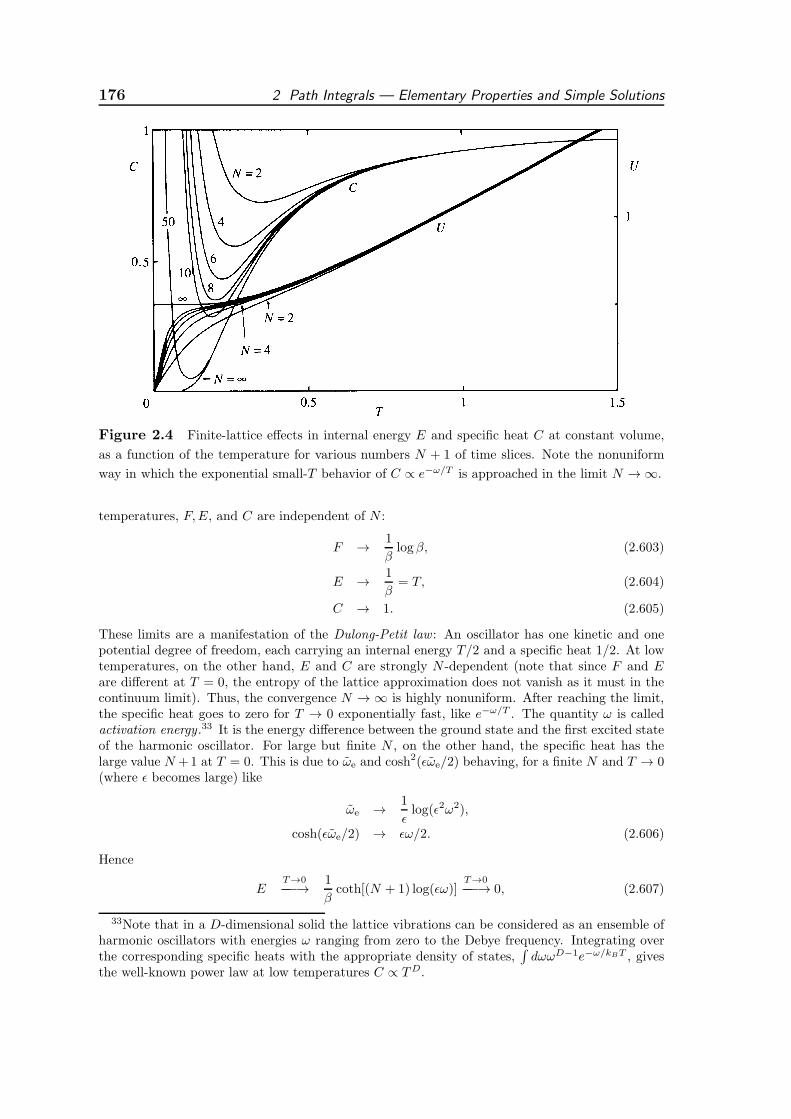
176 2 Path Integrals — Elementary Properties and Simple Solutions
Figure 2.4 Finite-lattice effects in internal energy E and specific heat C at constant volume,
as a function of the temperature for various numbers N + 1 of time slices. Note the nonuniform
way in which the exponential small-T behavior of C ∝ e−ω/T is approached in the limit N → ∞.
temperatures, F,E, and C are independent of N :
F → 1
βlog β, (2.603)
E → 1
β= T, (2.604)
C → 1. (2.605)
These limits are a manifestation of the Dulong-Petit law : An oscillator has one kinetic and onepotential degree of freedom, each carrying an internal energy T/2 and a specific heat 1/2. At lowtemperatures, on the other hand, E and C are strongly N -dependent (note that since F and Eare different at T = 0, the entropy of the lattice approximation does not vanish as it must in thecontinuum limit). Thus, the convergence N → ∞ is highly nonuniform. After reaching the limit,the specific heat goes to zero for T → 0 exponentially fast, like e−ω/T . The quantity ω is calledactivation energy.33 It is the energy difference between the ground state and the first excited stateof the harmonic oscillator. For large but finite N , on the other hand, the specific heat has thelarge value N +1 at T = 0. This is due to ωe and cosh2(ǫωe/2) behaving, for a finite N and T → 0(where ǫ becomes large) like
ωe → 1
ǫlog(ǫ2ω2),
cosh(ǫωe/2) → ǫω/2. (2.606)
Hence
ET→0−−−→ 1
βcoth[(N + 1) log(ǫω)]
T→0−−−→ 0, (2.607)
33Note that in a D-dimensional solid the lattice vibrations can be considered as an ensemble ofharmonic oscillators with energies ω ranging from zero to the Debye frequency. Integrating overthe corresponding specific heats with the appropriate density of states,
∫
dωωD−1e−ω/kBT , givesthe well-known power law at low temperatures C ∝ TD.
2.17 Time Evolution Amplitude of Freely Falling Particle 177
CT→0−−−→ N + 1. (2.608)
The reason for the nonuniform approach of the N → ∞ limit is obvious: If we expand (2.484) inpowers of ǫ, we find
ωe = ω
(
1 − 1
24ǫ2ω2 + . . .
)
. (2.609)
When going to low T at finite N the corrections are quite large, as can be seen by writing (2.609),with ǫ = hβ/(N + 1), as
ωe = ω
[
1 − 1
24
h2ω2
k2bT2(N + 1)2
+ . . .
]
. (2.610)
Note that (2.609) contains no corrections of the order ǫ. This implies that the convergence of
all thermodynamic quantities in the limit N → ∞, ǫ → 0 at fixed T is quite fast — one order in
1/N faster than we might at first expect [the Trotter formula (2.26) also shows the 1/N2 -behavior].
2.17 Time Evolution Amplitude of Freely Falling Particle
The gravitational potential of a particle on the surface of the earth is
V (x) = V0 +M g · x, (2.611)
where −g is the earth’s acceleration vector pointing towards the ground, and V0some constant. The equation of motion reads
x = −g, (2.612)
which is solved by
x = xa + va(t− ta) +g
2(t− ta)
2, (2.613)
with the initial velocity
va =xb − xa
tb − ta− g
2(tb − ta). (2.614)
Inserting this into the action
A =∫ tb
tadt(
M
2x2 − V0 − g · x
)
, (2.615)
we obtain the classical action
Acl = −V0(tb− ta)+M
2
(xb − xa)2
tb − ta− 1
2(tb− ta)g · (xb+xa)−
1
24(tb− ta)3g2. (2.616)
Since the quadratic part of (2.615) is the same as for a free particle, also the fluctu-ation factor is the same [see (2.130)], and we find the time evolution amplitude
(xbtb|xata) =1
√
2πih(tb − ta)/M3 e
− ihV0(tb−ta)
× exp
iM
2h
[
(xb − xa)2
tb − ta− (tb − ta)g · (xb + xa)−
1
12(tb − ta)
3g2
]
. (2.617)
178 2 Path Integrals — Elementary Properties and Simple Solutions
The potential (2.611) can be considered as a limit of a harmonic potential
V (x) = V0 +M
2ω2(x− x0)
2 (2.618)
for
ω → 0, x0 = −g/ω2 → −∞ ≈ g, V0 = −Mx20/2 = −Mg2/2ω4 → −∞, (2.619)
keepingg = −Mω2x0, (2.620)
and
v0 = V0 +M
2ω2x2
0 (2.621)
fixed. If we perform this limit in the amplitude (2.177), we find of course (2.617).The wave functions can be obtained most easily by performing this limiting
procedure on the wave functions of the harmonic oscillator. In one dimension, weset n = E/ω and find that the spectral representation (2.294) goes over into
(xbtb|xata) =∫
dEAE(xb)A∗E(xa)e
−i(E−v0)(tb−ta)/h, (2.622)
with the wave functions
AE(x) =1√lε
Ai(
x
l− E
ε
)
. (2.623)
Here ε ≡ (h2g2M/2)1/3 and l ≡ (h2/2M2g)1/3 = ε/Mg are the natural units ofenergy and length, respectively, and Ai(z) is the Airy function solving the differentialequation
Ai′′(z) = zAi(z), (2.624)
For positive z, the Airy function can be expressed in terms of modified Bessel func-tions Iν(ξ) and Kν(ξ):
34
Ai(z) =
√z
2[I−1/3(2z
3/2/3)− I1/3(2z3/2/3)] =
1
π
√
z
3K1/3
(
2z3/2/3)
. (2.625)
For large z, this falls off exponentially:
Ai(z) → 1
2√πz1/4
e−2z3/2/3, z → ∞. (2.626)
For negative z, an analytic continuation35
Iν(ξ) = e−πνi/2J(eπi/2ξ), − π < argξ ≤ π/2,
Iν(ξ) = e−πνi/2J(eπi/2ξ), π/2 < argξ ≤ π, (2.627)
34A compact description of the properties of Bessel functions is found in M. Abramowitz and I.Stegun, op. cit., Chapter 10. The Airy function is expressed in Formulas 10.4.14.
35I.S. Gradshteyn and I.M. Ryzhik, op. cit., Formulas 8.406.
2.18 Charged Particle in Magnetic Field 179
leads to
Ai(z) =1
3
√z[
J−1/3(2(−z)3/2/3) + J1/3(2(−z)3/2/3)]
, (2.628)
where J1/3(ξ) are ordinary Bessel functions. For large arguments, these oscillate like
Jν(ξ) →√
2
πξcos(ξ − πν/2− π/4) +O(ξ−1), (2.629)
from which we obtain the oscillating part of the Airy function
Ai(z) → 1√πz1/4
sin[
2(−z)3/2/3 + π/4]
, z → −∞. (2.630)
The Airy function has the simple Fourier representation
Ai(x) =∫ ∞
−∞
dk
2πei(xk+k3/3). (2.631)
In fact, the momentum space wave functions of energy E are
〈p|E〉 =√
l
εe−i(pE−p3/6M)l/εh (2.632)
fulfilling the orthogonality and completeness relations
∫
dp
2πh〈E ′|p〉〈p|E〉 = δ(E ′ −E),
∫
dE 〈p′|E〉〈E|p〉 = 2πhδ(p′ − p). (2.633)
The Fourier transform of (2.632) is equal to (2.623), due to (2.631).
2.18 Charged Particle in Magnetic Field
Having learned how to solve the path integral of the harmonic oscillator we are readyto study also a more involved harmonic system of physical importance: a chargedparticle in a magnetic field. This problem was first solved by L.D. Landau in 1930in Schrodinger theory.36
2.18.1 Action
The magnetic interaction of a particle of charge e is given by
Amag =e
c
∫ tb
tadt x(t) ·A(x(t)), (2.634)
where A(x) is the vector potential of the magnetic field. The total action is
A[x] =∫ tb
tadt[
M
2x2(t) +
e
cx(t) ·A(x(t))
]
. (2.635)
36L.D. Landau and E.M. Lifshitz, Quantum Mechanics , Pergamon, London, 1965.
180 2 Path Integrals — Elementary Properties and Simple Solutions
Suppose now that the particle moves in a homogeneous magnetic field B pointingalong the z-direction. Such a field can be described by a vector potential
A(x) = (0, Bx, 0). (2.636)
But there are other possibilities. The magnetic field
B(x) = ∇×A(x) (2.637)
as well as the magnetic interaction (2.634) are invariant under gauge transformations
A(x) → A(x) +∇Λ(x), (2.638)
where Λ(x) are arbitrary single-valued functions of x. As such they satisfy theSchwarz integrability condition [compare (1.40)–(1.41)]
(∂i∂j − ∂j∂i)Λ(x) = 0. (2.639)
For instance, the axially symmetric vector potential
A(x) =1
2B× x (2.640)
gives the same magnetic field; it differs from (2.636) by a gauge transformation
A(x) = A(x) +∇Λ(x), (2.641)
with the gauge function
Λ(x) = −1
2B xy. (2.642)
In the canonical form, the action reads
A[p,x] =∫ tb
tadt
p · x− 1
2M
[
p− e
cA(x)
]2
. (2.643)
The magnetic interaction of a point particle is thus included in the path integral bythe so-called minimal substitution of the momentum variable:
p → P ≡ p− e
cA(x). (2.644)
For the vector potential (2.636), the action (2.643) becomes
A[p,x] =∫ tb
tadt [p · x−H(p,x)] , (2.645)
with the Hamiltonian
H(p,x) =p2
2M+
1
8Mω2
Lx2 − 1
2ωLlz(p,x), (2.646)
2.18 Charged Particle in Magnetic Field 181
where x = (x, y) and p = (px, py) and
lz(p,x) = (x× p)z = xpy − ypx (2.647)
is the z-component of the orbital angular momentum. In a Schrodinger equation, thelast term in H(p,x) is diagonal on states with a given angular momentum aroundthe z-axis. We have introduced the field-dependent frequency
ωL =e
McB, (2.648)
called Landau frequency or cyclotron frequency . This can also be written in termsof the Bohr magneton
µB ≡ he
Mc, (2.649)
as
ωL = µBB/h. (2.650)
The first two terms in (2.646) describe a harmonic oscillator in the xy-plane witha field-dependent magnetic frequency
ωB ≡ ωL
2. (2.651)
Note that in the gauge gauge (2.636), the Hamiltonian would have the rotation-ally noninvariant form
H(p,x) =p2
2M+
1
2Mω2
Lx2 − ωLxpy (2.652)
rather than (2.646), implying oscillations of frequency ωL in the x-direction and afree motion in the y-direction.
The time-sliced form of the canonical action (2.643) reads
ANe =
N+1∑
n=1
pn(xn − xn−1)−1
2M
[
p2xn + (py n − Bxn)2 + p2zn
]
, (2.653)
and the associated time-evolution amplitude for the particle to run from xa to xb isgiven by
(xbtb|xata) =N∏
n=1
[∫
d3xn
]N+1∏
n=1
[
∫
d3pn(2πh)3
]
exp(
i
hAN
e
)
, (2.654)
with the time-sliced action
AN =N+1∑
n=1
pn(xn − xn−1)−1
2M
[
p2xn + (py n − Bxn)2 + p2zn
]
. (2.655)
182 2 Path Integrals — Elementary Properties and Simple Solutions
2.18.2 Gauge Properties
Note that the time evolution amplitude is not gauge-invariant. If we use the vectorpotential in some other gauge
A′(x) = A(x) +∇Λ(x), (2.656)
the action changes by a surface term
∆A =e
c
∫ tb
tadt x ·∇Λ(x) =
e
c[Λ(xb)− Λ(xa)]. (2.657)
The amplitude is therefore multiplied by a phase factor on both ends
(xbtb|xata)A → (xbtb|xata)A′ = eieΛ(xb)/ch(xbtb|xata)Ae−ieΛ(xa)/ch. (2.658)
For the observable particle distribution (x tb|x ta), the phase factors are obviouslyirrelevant. But all other observables of the system must also be independent of thephases Λ(x) which is assured if they correspond to gauge-invariant operators.
2.18.3 Time-Sliced Path Integration
Since the action AN contains the variables yn and zn only in the first term∑N+1
n=1 ipnxn, we can perform the yn, zn integrations and find a product of N ∆-functions in the y- and z-components of the momenta pn. If the projections of p tothe yz-plane are denoted by p′, the product is
(2πh)2δ(2)(
p′N+1 − p′
N
)
· · · (2πh)2δ(2) (p′2 − p′
1) . (2.659)
These allow performing all py n, pz n-integrals, except for one overall py, pz. The pathintegral reduces therefore to
(xbtb|xata) =∫ ∞
−∞
dpydpz(2πh)2
N∏
n=1
[∫ ∞
−∞dxn
]N+1∏
n=1
[
∫
dpxn
2πh
]
(2.660)
× exp
i
h
[
py(yb − ya) + pz(zb − za)− (tb − ta)p2z2M
]
exp(
i
hAN
x
)
,
where ANx is the time-sliced action involving only a one-dimensional path integral
over the x-component of the path, x(t), with the sliced action
ANx =
N+1∑
n=1
[
pxn(xn − xn−1)−p2xn
2M− 1
2M
(
py −e
cBxn
)2 ]
. (2.661)
This is the action of a one-dimensional harmonic oscillator with field-dependentfrequency ωB whose center of oscillation depends on py and lies at
x0 = py/MωL. (2.662)
2.18 Charged Particle in Magnetic Field 183
The path integral over x(t) is harmonic and known from (2.175):
(xbtb|xata)x0 =
√
MωL
2πih sinωL(tb − ta)
× exp(
i
h
MωL
2 sinωL(tb − ta)
[
(xb − x0)2 + (xa − x0)
2]
cosωL(tb − ta)
− 2(xb − x0)(xa − x0))
. (2.663)
Doing the pz-integral in (2.660), we arrive at the formula
(xbtb|xata) =1
√
2πih(tb − ta)/MeiM2h
(zb−za)2
tb−ta (x⊥b tb|x⊥
a ta), (2.664)
with the amplitude orthogonal to the magnetic field
(x⊥b tb|x⊥
a ta) ≡MωL
2πh
∫ ∞
−∞dx0 e
iMωLx0(yb−ya)/h(xbtb|xata)x0. (2.665)
After a quadratic completion in x0, the total exponent in (2.665) reads
iMωL
2h
[
−(x2b + x2a) tan[ωL(tb − ta)/2] + (xb − xa)2 1
sinωL(tb − ta)
]
−iMωL
htan[ωL(tb − ta)/2]
(
x0 −xb + xa
2− yb − ya
2 tan[ωL(tb − ta)/2]
)2
+iMωL
2h
[
(xb + xa)2
2tan[ωL(tb − ta)/2] +
(yb − ya)2
2 tan[ωL(tb − ta)/2]
]
+iMωL
2h(xb + xa)(yb − ya). (2.666)
The integration MωL
∫∞−∞ dx0/2πh removes the second term and results in a factor
MωL
2πh
√
πh
iMωL tan[ωL(tb − ta)/2]. (2.667)
By rearranging the remaining terms, we arrive at the amplitude
(xbtb|xata) =
√
M
2πih(tb − ta)
3ωL(tb − ta)/2
sin[ωL(tb − ta)/2]exp
[
i
h(Acl +Asf)
]
,
(2.668)
with an action
Acl =M
2
(zb − za)2
tb − ta+ωL
2cot[ωL(tb − ta)/2]
[
(xb − xa)2 + (yb − ya)
2]
+ ωL(xayb − xbya)
, (2.669)
and the surface term
Asf =MωL
2(xbyb − xaya) =
e
2cB xy
∣
∣
∣
b
a. (2.670)
184 2 Path Integrals — Elementary Properties and Simple Solutions
2.18.4 Classical Action
Since the action is harmonic, the amplitude is again a product of a phase eiAcl anda fluctuation factor. A comparison with (2.641) and (2.658) shows that the surfaceterm would be absent if the amplitude (xbtb|xata)A were calculated with the vectorpotential in the axially symmetric gauge (2.640). Thus Acl must be equal to theclassical action in this gauge. Indeed, the orthogonal part can be rewritten as
A⊥cl =
∫ tb
tadt
M
2
d
dt(xx+ yy) +
M
2[x(−x+ ωLy) + y(−y − ωLx)]
. (2.671)
The equations of motion are
x = ωLy, y = −ωLx, (2.672)
reducing the action of a classical orbit to
A⊥cl =
M
2(xx+ yy)
∣
∣
∣
tb
ta=M
2([xbxb − xaxa] + [ybyb − yaya]) . (2.673)
The orbits are easily determined. By inserting the two equations in (2.672) intoeach other we see that x and y perform independent oscillations:
˙x+ ω2Lx = 0, ˙y + ω2
Ly = 0. (2.674)
The general solution of these equations is
x =1
sinωL(tb − ta)[(xb − x0) sinωL(t− ta) − (xa − x0) sinωL(t− tb) ] + x0, (2.675)
y =1
sinωL(tb − ta)[(yb − y0) sinωL(t− ta) − (ya − y0) sinωL(t− tb) ] + y0, (2.676)
where we have incorporated the boundary condition x(ta,b) = xa,b, y(ta,b)= ya,b. The constants x0, y0 are fixed by satisfying (2.672). This gives
x0 =1
2
[
(xb + xa) + (yb − ya) cotωL
2(tb − ta)
]
, (2.677)
y0 =1
2
[
(yb + ya)− (xb− xa)cotωL
2(tb − ta)
]
. (2.678)
Now we calculate
xbxb =ωL
sinωL(tb − ta)xb [(x0 − xa) + (xb − x0) cosωL(tb − ta)] , (2.679)
xaxa =ωL
sinωL(tb − ta)xa [(x0 − xa) cosωL(tb − ta) + (xb − x0)] , (2.680)
and hence
xbxb − xaxa = ωLx0(xb + xa) tanωL
2(tb − ta)
+ωL
sinωL(tb − ta)
[
(x2b + x2a) cosωL(tb − ta)− 2xbxa]
=ωL
2
[
(xb − xa)2 cot
ωL
2(tb − ta) + (xb + xa)(yb − ya)
]
. (2.681)
2.18 Charged Particle in Magnetic Field 185
Similarly we find
ybyb − yaya = ωLy0(yb + ya) tanωL
2(tb − ta)
+ωL
sinωL(tb − ta)[(y2b + y2a) cosωL(tb − ta)− 2ybya]
=ωL
2
[
(yb − ya)2 cot
ωL
2(tb − ta)− (xb − xa)(yb + ya)
]
. (2.682)
Inserted into (2.673), this yields the classical action for the orthogonal motion
A⊥cl =
M
2
ωL
2cot[ωL(tb − ta)/2]
[
(xb − xa)2 + (yb − ya)
2]
+ ωL(xayb − xbya)
,
(2.683)
which is indeed the orthogonal part of the action (2.669).
2.18.5 Translational Invariance
It is interesting to see how the amplitude ensures the translational invariance of allphysical observables. The first term in the classical action is trivially invariant. Thelast term reads
∆A =MωL
2(xayb − xbya). (2.684)
Under a translation by a distance d,
x → x + d, (2.685)
this term changes by
MωL
2[dx(yb − ya) + dy(xa − xb)] =
MωL
2[(d× x)b − (d× x)a]z (2.686)
causing the amplitude to change by a pure gauge transformation as
(xbtb|xata) → eieΛ(xb)/ch(xbtb|xata)e−ieΛ(xa)/ch, (2.687)
with the phase
Λ(x) = −MωLhc
2e[d× x]z . (2.688)
Since observables involve only gauge-invariant quantities, such transformations areirrelevant.
This will be done in 2.23.3.
186 2 Path Integrals — Elementary Properties and Simple Solutions
2.19 Charged Particle in Magnetic Field plus
Harmonic Potential
For application in Chapter 5 we generalize the above magnetic system by adding aharmonic oscillator potential, thus leaving the path integral solvable. For simplicity,we consider only the orthogonal part of the resulting system with respect to themagnetic field. Omitting orthogonality symbols, the Hamiltonian is the same as in(2.646). Without much more work we may solve the path integral of a more generalsystem in which the harmonic potential in (2.646) has a different frequency ω 6= ωL,and thus a Hamiltonian
H(p,x) =p2
2M+
1
2Mω2x2 − ωBlz(p,x). (2.689)
The associated Euclidean action
Ae[p,x] =∫ τb
τadτ [−ip · x+H(p,x)] (2.690)
has the Lagrangian form
Ae[x] =∫ hβ
0dτ
M
2x2(τ) +
1
2M(ω2 − ω2
B)x2(τ)− iMωB[x(τ)× x(τ)]z
.
(2.691)
At this point we observe that the system is stable only for ω ≥ ωB. The action(2.691) can be written in matrix notation as
Acl =∫ hβ
0dτ
[
M
2
d
dτ(xx) +
M
2xT Dω2,B x
]
, (2.692)
where Dω2,B is the 2× 2 -matrix
Dω2,B(τ, τ′) ≡
(
−∂2τ + ω2 − ω2B −2iωB∂τ
2iωB∂τ −∂2τ + ω2 − ω2B
)
δ(τ − τ ′). (2.693)
Since the path integral is Gaussian, we can immediately calculate the partitionfunction
Z =1
(2πh/M)2detD
−1/2ω2,B . (2.694)
By expanding Dω2,B(τ, τ′) in a Fourier series
Dω2,B(τ, τ′) =
1
hβ
∞∑
m=−∞
Dω2,B(ωm)e−iωm(τ−τ ′), (2.695)
we find the Fourier components
Dω2,B(ωm) =
(
ω2m + ω2 − ω2
B −2ωBωm
2ωBωm ω2m + ω2 − ω2
B
)
, (2.696)
2.19 Charged Particle in Magnetic Field plus Harmonic Potential 187
with the determinants
det Dω2,B(ωm) = (ω2m + ω2 − ω2
B)2 + 4ω2
Bω2m. (2.697)
These can be factorized as
det Dω2,B(ωm) = (ω2m + ω2
+)(ω2m + ω2
−), (2.698)
withω± ≡ ω ± ωB. (2.699)
The eigenvectors of Dω2,B(ωm) are
e+ =1√2
(
1i
)
, e− = − 1√2
(
1−i
)
, (2.700)
with eigenvalues
d± = ω2m + ω2 ± 2iωmωB = (ωm + iω±)(ωm − iω∓). (2.701)
Thus the right- and left-circular combinations x± = ±(x ± iy)/√2 diagonalize the
Lagrangian (2.692) to
Acl =∫ hβ
0dτ
M
2
d
dτ
(
x∗+x+ + x∗−x−)
+M
2
[
x∗+(−∂τ − ω+)(−∂τ + ω−)x+ + x∗−(−∂τ − ω−)(−∂τ + ω+)x−]
. (2.702)
Continued back to real times, the components x±(t) are seen to oscillate indepen-dently with the frequencies ω±.
The factorization (2.698) makes (2.702) an action of two independent harmonicoscillators of frequencies ω±. The associated partition function has therefore theproduct form
Z =1
2 sinh (hβω+/2)
1
2 sinh (hβω−/2). (2.703)
For the original system of a charged particle in a magnetic field discussed inSection 2.18, the partition function is obtained by going to the limit ω → ωB inthe Hamiltonian (2.689). Then ω− → 0 and the partition function (2.703) diverges,since the system becomes translationally invariant in space. From the mnemonicreplacement rule (2.361) we see that in this limit we must replace the relevantvanishing inverse frequency by an expression proportional to the volume of thesystem. The role of ω2 in (2.361) is played here by the frequency in front of thex2-term of the Lagrangian (2.691). Since there are two dimensions, we must replace
1
ω2 − ω2B
−−−→ω→ωB
1
2ωω−
−−−→ω−→0
β
2π/MV2, (2.704)
and thus
Z −−−→ω−→0
1
2 sinh (hβω)
V2λ2ω, (2.705)
where λω is the quantum-mechanical length scale in Eqs. (2.303) and (2.359) of theharmonic oscillator.
188 2 Path Integrals — Elementary Properties and Simple Solutions
2.20 Gauge Invariance and Alternative Path Integral
Representation
The action (2.635) of a particle in an external ordinary potential V (x, t) and a vector potentialA(x, t) can be rewritten with the help of an arbitrary space- and time-dependent gauge functionΛ(x, t) in the following form:
A[x] =
∫ tb
ta
dt
M
2x2 +
e
cx(t)[A(x, t) + ∇Λ(x, t)]−V (x, t)+
e
c∂tΛ(x, t)
− e
c[Λ(xb, tb) − Λ(xa, ta)] . (2.706)
The Λ(x, t)-terms inside the integral are canceled by the last two surface terms making the actionindependent of Λ(x, t).
We may now choose a particular function Λ(x, t) equal to c/e-times the classical action A(x, t)which solves the Hamilton-Jacobi equation (1.65), i.e.,
1
2M
[
∇A(x, t) − e
cA(x, t)
]2
+ ∂tA(x, t) + V (x, t) = 0. (2.707)
Then we obtain the following alternative expression for the action:
A[x] =
∫ tb
ta
dt1
2M
[
M x−∇A(x, t) +e
cA(x, t)
]2
+ A(xb, tb) −A(xa, ta). (2.708)
For two infinitesimally different solutions of the Hamilton-Jacobi equation, the difference betweenthe associated action functions δA satisfies the differential equation
v ·∇δA + ∂tδA = 0, (2.709)
where v is the classical velocity field
v(x, t) ≡ (1/M)[
∇A(x, t) − e
cA(x, t)
]
. (2.710)
The differential equation (2.709) expresses the fact that two solutions A(x, t) for which the particleenergy and momenta at x and t differ by δE and δp, respectively, satisfy the kinematic relationδE = p · δp/M = xcl ·∇δA. This follows directly from E = p2/2M . The so-constrained variationsδE and δp leave the action (2.708) invariant.
A sequence of changes δA of this type can be used to make the function A(x, t) coincide withthe action A(x, t;xa, ta) of paths which start out from xa, ta and arrive at x, t. In terms of thisaction function, the path integral representation of the time evolution amplitude takes the form
(xbtb|xata) = eiA(xb,tb;xa,ta)/h
∫ x(tb)=xb
x(ta)=xa
Dx (2.711)
×exp
i
h
∫ tb
ta
dt1
2M
[
M x−∇A(x, t;xa, ta) +e
cA(x, t)
]2
or, using v(x(t), t),
(xbtb|xata) = eiA(xb,tb;xa,ta)/h
∫ x(tb)=xb
x(ta)=xa
Dx exp
[
i
h
∫ tb
ta
dtM
2(x− v)
2
]
.
(2.712)
2.21 Velocity Path Integral 189
The fluctuations are now controlled by the deviations of the instantaneous velocity x(t) from localvalue of the classical velocity field v(x, t). Since the path integral attempts to keep the deviationsas small as possible, we call v(x, t) the desired velocity of the particle at x and t. Introducingmomentum variables p(t), the amplitude may be written as a phase space path integral
(xbtb|xata) = eiA(xb,tb;xa,ta)/h
∫ x(tb)=xb
x(ta)=xa
D′x
∫ Dp
2πh
× exp
(
i
h
∫ tb
ta
dt
p(t) [x(t) − v(x(t), t)] − 1
2Mp2(t)
)
, (2.713)
which will be used in Section 18.15 to give a stochastic interpretation of quantum processes.
2.21 Velocity Path Integral
There exists yet another form of writing the path integral in which the fluctuating velocities play afundamental role and which will later be seen to be closely related to path integrals in the so-calledstochastic calculus to be introduced in Sections 18.13 and 18.640. We observe that by rewritingthe path integral as
(xbtb|xata)=
∫
D3x δ
(
xb−xa−∫ tb
ta
dt x(t)
)
exp
i
h
∫ tb
ta
dt
[
M
2x2−V (x)
]
, (2.714)
the δ-function allows us to include the last variable xn in the integration measure of the time-slicedversion of the path integral. Thus all time-sliced time derivatives (xn+1 − xn)/ǫ for n = 0 to Nare integrated over implying that they can be considered as independent fluctuating variables vn.In the potential, the dependence on the velocities can be made explicit by inserting
x(t) = xb −∫ tb
t
dtv(t), (2.715)
x(t) = xa +
∫ t
ta
dtv(t), (2.716)
x(t) = X +1
2
∫ tb
ta
dt′ v(t′)ǫ(t′ − t), (2.717)
where
X ≡ xb + xa
2(2.718)
is the average position of the endpoints and ǫ(t− t′) is the antisymmetric combination of Heavisidefunctions introduced in Eq. (1.315).
In the first replacement, we obtain the velocity path integral
(xbtb|xata)=
∫
D3v δ
(
xb−xa−∫ tb
ta
dtv(t)
)
exp
i
h
∫ tb
ta
dt
[
M
2v2−V
(
xb−∫ tb
t
dtv(t)
)]
. (2.719)
The measure of integration is normalized to make
∫
D3v exp
i
h
∫ tb
ta
dt
[
M
2v2
]
= 1. (2.720)
The correctness of this normalization can be verified by evaluating (2.719) for a free particle.Inserting the Fourier representation for the δ-function
δ
(
xb − xa −∫ tb
ta
dtv(t)
)
=
∫
d3p
(2πi)3exp
[
i
hp
(
xb − xa −∫ tb
ta
dtv(t)
)]
, (2.721)
190 2 Path Integrals — Elementary Properties and Simple Solutions
we can complete the square in the exponent and integrate out the v-fluctuations using (2.720) toobtain
(xbtb|xata) =
∫
d3p
(2πi)3exp
i
h
[
p (xb − xa) −p2
2M(tb − ta)
]
. (2.722)
This is precisely the spectral representation (1.333) of the free-particle time evolution amplitude(1.335) [see also Eq. (2.53)].
A more symmetric velocity path integral is obtained by choosing the third replacement (2.717).This leads to the expression
(xbtb|xata) =
∫
D3v δ
(
∆x−∫ tb
ta
dtv(t)
)
exp
i
h
∫ tb
ta
dtM
2v2
× exp
− i
h
∫ tb
ta
dt V
(
X +1
2
∫ tb
ta
dt′ v(t′)ǫ(t′ − t)
)
. (2.723)
The velocity representations are particularly useful if we want to know integrated amplitudes suchas
∫
d3xa (xbtb|xata) =
∫
D3v exp
i
h
∫ tb
ta
dtM
2v2
.
× exp
− i
h
∫ tb
ta
dtV
(
xb −1
2
∫ tb
t
dt′ v(t′)
)
, (2.724)
which will be of use in the next section.
2.22 Path Integral Representation of the Scattering Matrix
In Section 1.16 we have seen that the description of scattering processes requires several nontriviallimiting procedures on the time evolution amplitude. Let us see what these procedures yield whenapplied to the path integral representation of this amplitude.
2.22.1 General Development
Formula (1.474) for the scattering matrix expressed in terms of the time evolution operator inmomentum space has the following path integral representation:
〈pb|S|pa〉 ≡ limtb−ta→∞
ei(Ebtb−Eata)/h
∫
d3xb
∫
d3xae−i(pbxb−paxa)/h(xbtb|xata). (2.725)
Introducing the momentum transfer q ≡ (pb − pa), we rewrite e−i(pbxb−paxa)/h ase−iqxb/he−ipa(xb−xa)/h, and observe that the amplitude including the exponential prefactore−ipa(xb−xa)/h has the path integral representation:
e−ipa(xb−xa)/h(xbtb|xata) =
∫
D3x exp
i
h
∫ tb
ta
dt
[
M
2x2 − pax− V (x)
]
. (2.726)
The linear term in x is eliminated by shifting the path from x(t) to
y(t) = x(t) − pa
Mt (2.727)
leading to
e−ipa(xb−xb)/h(xbtb|xata)=e−ip2
a(tb−ta)/2Mh
∫
D3y exp
i
h
∫ tb
ta
dt
[
M
2y2−V
(
y+P
Mt
)]
.
(2.728)
2.22 Path Integral Representation of the Scattering Matrix 191
Inserting everything into (2.725) we obtain
〈pb|S|pa〉 ≡ limtb−ta→∞
eiq2tb/2Mh
∫
d3yb e−iqyb/h
∫
d3ya
×∫
D3y exp
i
h
∫ tb
ta
dt
[
M
2y2−V
(
y +pa
Mt)
]
. (2.729)
In the absence of an interaction, the path integral over y(t) gives simply
∫
d3ya1
√
2πhi(tb − ta)/Mexp
[
i
h
M
2
(yb − ya)2
tb − ta)
]
= 1, (2.730)
and the integral over ya yields
〈pb|S|pa〉|V ≡0 = limtb−ta→∞
eiq2(tb−ta)/8Mh(2πh)3δ(3)(q) = (2πh)3δ(3)(pb − pa), (2.731)
which is the contribution from the unscattered beam to the scattering matrix in Eq. (1.477).The first-order contribution from the interaction reads, after a Fourier decomposition of the
potential,
〈pb|S1|pa〉 = − i
hlim
tb−ta→∞eiq
2tb/2Mh
∫
d3yb e−iqyb/h
∫
d3Q
(2πh)3V (Q)
∫
d3ya
×∫ tb
ta
dt′ exp
(
i
h
paQ
Mt′)∫
D3y exp
i
h
∫ tb
ta
dt
[
M
2y2+ δ(t′−t)Qy
]
. (2.732)
The harmonic path integral was solved in one dimension for an arbitrary source j(t) in Eq. (3.168).For ω = 0 and the particular source j(t) = δ(t′ − t)Q the result reads, in three dimensions,
1√
2πih(tb − ta)/M3 exp
[
i
h
M
2
(yb − ya)2
tb − ta
]
× exp
(
i
h
1
tb − ta
[yb(t′ − ta) + ya(tb − t′)]Q− 1
2M(tb − t′)(t′ − ta)Q
2
)
. (2.733)
Performing here the integral over ya yields
exp
i
hQyb
exp
− i
h
1
2M(tb − t′)Q2
. (2.734)
The integral over yb in (2.732) leads now to a δ-function (2πh)3δ(3)(Q − q), such that the expo-nential prefactor in (2.732) is canceled by part of the second factor in (2.734).
In the limit tb− ta → ∞, the integral over t′ produces a δ-function 2πhδ(pbQ/M +Q2/2M) =2πhδ(Eb − Ea) which enforces the conservation of energy. Thus we find the well-known Bornapproximation
〈pb|S1|pa〉 = −2πiδ(Eb − Ea)V (q). (2.735)
In general, we subtract the unscattered particle term (2.731) from (2.729), to obtain a pathintegral representation for the T -matrix [for the definition recall (1.477)]:
2πhiδ(Eb − Ea)〈pb|T |pa〉 ≡ − limtb−ta→∞
eiq2tb/2Mh
∫
d3yb e−iqyb/h
∫
d3ya
×∫
D3y exp
(
i
h
∫ tb
ta
dtM
2y2
)
exp
[
− i
h
∫ tb
ta
dt V(
y +pa
Mt)
]
− 1
. (2.736)
192 2 Path Integrals — Elementary Properties and Simple Solutions
It is preferable to find a formula which does not contain the δ-function of energy conservation asa factor on the left-hand side. In order to remove this we observe that its origin lies in the time-translational invariance of the path integral in the limit tb−ta → ∞. If we go over to a shifted timevariable t → t + t0, and change simultaneously y → y − pat0/M , then the path integral remainsthe same except for shifted initial and final times tb + t0 and ta + t0. In the limit tb − ta → ∞, theintegrals
∫ tb+t0ta+t0
dt can be replaced again by∫ tbta
dt. The only place where a t0-dependence remains
is in the prefactor e−iqyb/h which changes to e−iqyb/heiqpat0/Mh. Among all path fluctuations, thereexists one degree of freedom which is equivalent to a temporal shift of the path. This is equivalent toan integral over t0 which yields a δ-function 2πhδ (qpa/M) = 2πhδ (Eb − Ea). We only must makesure to find the relation between this temporal shift and the corresponding measure in the pathintegral. This is obviously a shift of the path as a whole in the direction pa ≡ pa/|pa|. The formalway of isolating this degree of freedom proceeds according to a method developed by Faddeev andPopov37 by inserting into the path integral (2.729) the following integral representation of unity:
1 =|pa|M
∫ ∞
−∞
dt0 δ (pa(yb + pat0/M)) . (2.737)
In the following, we shall drop the subscript a of the incoming beam, writing
p ≡ pa, p ≡ |pa| = |pb|. (2.738)
After the above shift in the path integral, the δ-function in (2.737) becomes δ (payb) inside the pathintegral, with no t0-dependence. The integral over t0 can now be performed yielding the δ-functionin the energy. Removing this from the equation we obtain the path integral representation of theT -matrix
〈pb|T |pa〉 ≡ ip
Mlim
tb−ta→∞eiq
2(tb−ta)/8Mh
∫
d3yb δ (payb) e−iqyb/h
∫
d3ya
×∫
D3y exp
(
i
h
∫ tb
ta
dtM
2y2
)
exp
[
− i
h
∫ tb
ta
dt V
(
y+P
Mt
)]
−1
. (2.739)
At this point it is convenient to go over to the velocity representation of the path integral (2.723).This enables us to perform trivially the integral over yb, and we obtain the y version of (2.724).The δ-function enforces a vanishing longitudinal component of yb. The transverse component ofyb will be denoted by b:
b ≡ yb − (payb)p/a. (2.740)
Hence we find the path integral representation
〈pb|T |pa〉 ≡ ip
Mlim
tb−ta→∞eiq
2tb/2Mh
∫
d2b e−iqb/h
×∫
D3v exp
(
i
h
∫ tb
ta
dtM
2v2
)
[
eiχb,p[v] − 1]
, (2.741)
where the effect of the interaction is contained in the scattering phase
χb,p[v] ≡ − 1
h
∫ tb
ta
dt V
(
b +p
Mt−∫ tb
t
dt′ v(t′)
)
. (2.742)
We can go back to a more conventional path integral by replacing the velocity paths v(t) by
y(t) = −∫ tbt v(t). This vanishes at t = tb. Equivalently, we can use paths z(t) with periodic
boundary conditions and subtract from these z(tb) = zb.From 〈pb|T |pa〉 we obtain the scattering amplitude fpbpa
, whose square gives the differentialcross section, by multiplying it with a factor −M/2πh [see Eq. (1.497)].
37L.D. Faddeev and V.N. Popov, Phys. Lett. B 25 , 29 (1967).

2.22 Path Integral Representation of the Scattering Matrix 193
Note that in the velocity representation, the evaluation of the harmonic path integral integratedover ya in (2.732) is much simpler than before where we needed the steps (2.733), (2.734). Afterthe Fourier decomposition of V (x) in (2.742), the relevant integral is
∫
D3v exp
i
h
∫ tb
ta
dt
[
M
2v2−Θ(tb− t′)Qv
]
=e− i
2Mh
∫
tb
tadtΘ2(tb−t
′)Q2
=e−i
2Mh(tb−t′)Q2
. (2.743)
The first factor in (2.734) comes directly from the argument Y in the Fourier representation of thepotential
V
(
yb +p
Mt−
∫ tb
t
dt′ v(t′)
)
in the velocity representation of the S-matrix (2.729).
2.22.2 Improved Formulation
The prefactor eiq2tb/2Mh in Formula (2.741) is an obstacle to taking a more explicit limit tb−ta → ∞
on the right-hand side. To overcome this, we represent this factor by an auxiliary path integral38
over some vector field w(t):
eiq2tb/2Mh =
∫
D3w exp
[
− i
h
∫ tb
ta
dtM
2w2(t)
]
ei∫
tb
tadtΘ(t)w(t)q/h
. (2.744)
The last factor changes the exponential e−iqb/h in (2.741) into e−iq
[
b+∫
tb
tadtΘ(t)w(t)
]
/h. Since b is
a dummy variable of integration, we can equivalently replace b → bw ≡ b−∫ tbta
dtΘ(t)w(t) in the
scattering phase χb,p[v] and remain with
fpbpa= lim
tb−ta→∞
p
2πih
∫
d2b e−iqb/h
∫
D3w
×∫
D3v exp
[
i
h
∫ ∞
−∞
dtM
2
(
v2 −w2)
]
[exp (iχbw,p) − 1] . (2.745)
The scattering phase in this expression can be calculated from formula (2.742) with the integraltaken over the entire t-axis:
χbw,p[v,w] = − 1
h
∫ ∞
−∞
dt V
(
b +p
Mt−∫ tb
ta
dt′ [Θ(t′−t)v(t′) − Θ(t′)w(t′)]
)
. (2.746)
The fluctuations of w(t) are necessary to correct for the fact that the outgoing particle does notrun, on the average, with the velocity p/M = pa/M but with velocity pb/M = (p + q)/M .
We may also go back to a more conventional path integral by inserting y(t) = −∫ tbt
v(t) and
setting similarly z(t) = −∫ tbt
w(t). Then we obtain the alternative representation
fpbpa= lim
tb−ta→∞
p
2πih
∫
d2b e−iqb/h
∫
d3ya
∫
d3za
×∫
D3y
∫
D3z exp
[
i
h
∫ tb
ta
dtM
2
(
y2 − z2)
]
[
eiχbz,p[y] − 1]
, (2.747)
38See R. Rosenfelder, notes of a lecture held at the ETH Zurich in 1979: Pfadintegrale in der
Quantenphysik , 126 p., PSI Report 97-12, ISSN 1019-0643, and Lecture held at the 7th Int. Conf.on Path Integrals in Antwerpen, Path Integrals from Quarks to Galaxies , 2002; Phys. Rev. A 79,012701 (2009).
194 2 Path Integrals — Elementary Properties and Simple Solutions
with
χbz,p[y] ≡ − 1
h
∫ tb
ta
dt V(
b +p
Mt + y(t) − z(0)
)
, (2.748)
where the path integrals run over all paths with yb = 0 and zb = 0. In Section 3.26 this pathintegral will be evaluated perturbatively.
2.22.3 Eikonal Approximation to the Scattering Amplitude
To lowest approximation, we neglect the fluctuating variables y(t) and z(t) in (2.748). Since theintegral
∫
d3ya
∫
d3za
∫
D3y
∫
D3z exp
[
i
h
∫ tb
ta
dtM
2
(
y2 − z2)
]
(2.749)
in (2.747) has unit normalization [recall the calculation of (2.734)], we obtain directly the eikonalapproximation to the scattering amplitude
f eipbpa
≡ p
2πih
∫
d2b e−iqb/h[
exp(
iχeib,p
)
− 1]
, (2.750)
with
χeib,p ≡ − 1
h
∫ ∞
−∞
dt V(
b +p
Mt)
. (2.751)
The time integration can be converted into a line integration along the direction of the incomingparticles by introducing a variable z ≡ pt/M . Then we can write
χeib,p ≡ −M
p
1
h
∫ ∞
−∞
dz V (b + pz) . (2.752)
If V (x) is rotationally symmetric, it depends only on r ≡ |x|. Then we shall write the potentialas V (r) and calculate (2.752) as the integral
χeib,p ≡ −M
p
1
h
∫ ∞
−∞
dz V(
√
b2 + z2)
. (2.753)
Inserting this into (2.750), we can perform the integral over all angles between q and b using theformula
1
2π
∫ π
−π
dθ exp
(
i
hqb cos θ
)
= J0(qb), (2.754)
where J0(ξ) is the Bessel function, and find
f eipbpa
=p
ih
∫
db b J0(qb)[
exp(
iχeib,p
)
− 1]
. (2.755)
The variable of integration b coincides with the impact parameter b introduced in Eq. (1.500). Theresult (2.755) is precisely the eikonal approximation (1.500) with χei
b,p/2 playing the role of thescattering phases δl(p) of angular momentum l = pb/h:
χeib,p = 2iδpb/h(p). (2.756)
2.23 Heisenberg Operator Approach to Time Evolution
Amplitude
An interesting alternative to the path integral derivation of the time evolution amplitudes ofharmonic systems is based on quantum mechanics in the Heisenberg picture. It bears a closesimilarity with the path integral derivation in that it requires solving the classical equations ofmotion with given initial and final positions to obtain the exponential of the classical action eiA/h.The fluctuation factor, however, which accompanies this exponential is obtained quite differentlyfrom commutation rules of the operatorial orbits at different times as we shall now demonstrate.
2.23 Heisenberg Operator Approach to Time Evolution Amplitude 195
2.23.1 Free Particle
We want to calculate the matrix element of the time evolution operator
(x t|x′ 0) = 〈x|e−iHt/h|x′〉, (2.757)
where H is the Hamiltonian operator
H = H(p) =p2
2M. (2.758)
We shall calculate the time evolution amplitude (2.757) by solving the differential equation
ih∂t〈x t|x′ 0〉 ≡ 〈x|H e−iHt/h|x′〉 = 〈x|e−iHt/h[
eiHt/hH e−iHt/h]
|x′〉= 〈x t|H(p(t))|x′ 0〉. (2.759)
The argument contains now the time-dependent Heisenberg picture of the operator p. The evalu-ation of the right-hand side will be based on re-expressing the operator H(p(t)) as a function ofinitial and final position operators in such a way that all final position operators stand to the leftof all initial ones:
H = H(x(t), x(0); t). (2.760)
Then the matrix elements on the right-hand side can immediately be evaluated using the eigenvalueequations
〈x t|x(t) = x〈x t|, x(0)|x′ 0〉 = x′|x′ 0〉, (2.761)
as being
〈x t|H(x(t), x(0); t)|x 0〉 = H(x,x′; t)〈x t|x′ 0〉, (2.762)
and the differential equation (2.759) becomes
ih∂t〈x t|x′ 0〉 ≡ H(x,x′; t)〈x t|x′ 0〉, (2.763)
or
〈x t|x′ 0〉 = C(x,x′)E(x,x′; t) ≡ C(x,x′)e−i∫
tdt′ H(x,x′;t′)/h
. (2.764)
The prefactor C(x,x′) contains a possible constant of integration resulting from the time integralin the exponent.
The Hamiltonian operator is brought to the time-ordered form (2.760) by solving the Heisen-berg equations of motion
dx(t)
dt=
i
h
[
H, x(t)]
=p(t)
M, (2.765)
dp(t)
dt=
i
h
[
H, p(t)]
= 0. (2.766)
The second equation shows that the momentum is time-independent:
p(t) = p(0), (2.767)
so that the first equation is solved by
x(t) − x(0) = tp(t)
M, (2.768)

196 2 Path Integrals — Elementary Properties and Simple Solutions
which brings (2.758) to
H =M
2t2[x(t) − x(0)]
2. (2.769)
This is not yet the desired form (2.760) since there is one factor which is not time-ordered. Theproper order is achieved by rewriting H as
H =M
2t2
x2(t) − 2x(t)x(0) + x2(0) + [x(t), x(0)]
, (2.770)
and calculating the commutator from Eq. (2.768) and the canonical commutation rule [pi, xj ] =−ihδij as
[x(t), x(0)] = − ih
MDt, (2.771)
so that we find the desired expression
H = H(x(t), x(0); t) =M
2t2[
x2(t) − 2x(t)x(0) + x2(0)]
− ihD
2t. (2.772)
Its matrix elements (2.762) can now immediately be written down:
H(x,x′; t) =M
2t2(x− x′)
2 − ihD
2t. (2.773)
From this we find directly the exponential factor in (2.764)
E(x,x′; t) = e−i∫
dtH(x,x′;t)/h = exp
[
i
h
M
2t(x− x′)
2 − D
2log t
]
. (2.774)
Inserting (2.774) into Eq. (2.764), we obtain
〈x t|x′ 0〉 = C(x,x′)1
tD/2exp
[
i
h
M
2t(x− x′)
2]
. (2.775)
A possible constant of integration in (2.774) depending on x,x′ is absorbed in the prefactor C(x,x′).This is fixed by differential equations involving x:
−ih∇〈x t|x′ 0〉 = 〈x|pe−iHt/h|x′〉 = 〈x|e−iHt[
eiHt/hpe−iHt/h]
|x′〉 = 〈x t|p(t)|x′ 0〉.
ih∇′〈x t|x′ 0〉 = 〈x|e−iHt/hp|x′〉〈x t|p(0)|x′ 0〉. (2.776)
Inserting (2.768) and using the momentum conservation (2.767), these become
−ih∇〈x t|x′ 0〉 =M
t(x− x′) 〈x t|x′ 0〉,
ih∇′〈x t|x′ 0〉 =M
t(x− x′) 〈x t|x′ 0〉. (2.777)
Inserting here the previous result (2.775), we obtain the conditions
−i∇C(x,x′) = 0, i∇′C(x,x′) = 0, (2.778)
which are solved only by a constant C. The constant, in turn, is fixed by the initial condition
limt→0
〈x t|x′ 0〉 = δ(D)(x− x′), (2.779)
to be
C =
√
M
2πih
D
, (2.780)
so that we find the correct free-particle amplitude (2.74)
〈x t|x′ 0〉 ≡√
M
2πiht
D
exp
[
i
h
M
2t(x− x′)2
]
. (2.781)
Note that the fluctuation factor 1/tD/2 emerges in this approach as a consequence of the commu-tation relation (2.771).
2.23 Heisenberg Operator Approach to Time Evolution Amplitude 197
2.23.2 Harmonic Oscillator
Here we are dealing with the Hamiltonian operator
H = H(p, x) =p2
2M+
Mω2
2x2, (2.782)
which has to be brought again to the time-ordered form (2.760). We must now solve the Heisenbergequations of motion
dx(t)
dt=
i
h
[
H, x(t)]
=p(t)
M, (2.783)
dp(t)
dt=
i
h
[
H, p(t)]
= −Mω2x(t). (2.784)
By solving these equations we obtain [compare (2.158)]
p(t) = Mω
sinωt[x(t) cosωt− x(0)] . (2.785)
Inserting this into (2.782), we obtain
H =Mω2
2 sin2 ωt
[x(t) cosωt− x(0)]2+ sin2 ωt x2(t)
, (2.786)
which is equal to
H =Mω2
2 sin2 ωt
x2(t) + x2(0) − 2 cosωt x(t)x(0) + cosωt [x(t), x(0)]
. (2.787)
By commuting Eq. (2.785) with x(t), we find the commutator [compare (2.771)]
[x(t), x(0)] = − ih
MD
sinωt
ω, (2.788)
so that we find the matrix elements of the Hamiltonian operator in the form (2.762) [compare(2.773)]
H(x,x′; t) =Mω2
2 sin2 ωt
(
x2 + x′2 − 2 cosωtxx′)
− ihD
2ω cotωt. (2.789)
This has the integral [compare (2.774)]
∫
dtH(x,x′; t) = − Mω
2 sinωt
[(
x2 + x′2)
cosωt− 2xx′]
− ihD
2log
sinωt
ω. (2.790)
Inserting this into Eq. (2.764), we find precisely the harmonic oscillator amplitude (2.177), apartfrom the factor C(x,x′). This is again determined by the differential equations (2.776), leavingonly a simple normalization factor fixed by the initial condition (2.779) with the result (2.780).
Again, the fluctuation factor has its origin in the commutator (2.788).
2.23.3 Charged Particle in Magnetic Field
We now turn to a charged particle in three dimensions in a magnetic field treated in Section 2.18,where the Hamiltonian operator is most conveniently expressed in terms of the operator of thecovariant momentum (2.644),
P ≡ p− e
cA(x), (2.791)
198 2 Path Integrals — Elementary Properties and Simple Solutions
as [compare (2.643)]
H = H(p, x) =P2
2M. (2.792)
In the presence of a magnetic field, its components do not commute but satisfy the commutationrules:
[Pi, Pj ] = −e
c[pi, Aj ] −
e
c[Ai, pj] = i
eh
c(∇iAj −∇jAi) = i
eh
cBij , (2.793)
where Bij = ǫijkBK is the usual antisymmetric tensor representation of the magnetic field.We now have to solve the Heisenberg equations of motion
dx(t)
dt=
i
h
[
H, x (t)]
=P(t)
M(2.794)
dP(t)
dt=
i
h
[
H, P(t)]
=e
McB(x(t))P(t) + i
eh
Mc∇jBji(x(t)), (2.795)
where B(x(t))P(t) is understood as the product of the matrix Bij(x(t)) with the vector P. In aconstant field, where Bij(x(t)) is a constant matrix Bij , the last term in the second equation isabsent and we find directly the solution
P(t) = eΩLtP(0), (2.796)
where ΩL is a matrix version of the Landau frequency (2.648)
ΩL ij ≡e
McBij , (2.797)
which can also be rewritten with the help of the Landau frequency vector
!L ≡ e
McB (2.798)
and the 3 × 3-generators of the rotation group
(Lk)ij ≡ −iǫkij (2.799)
asΩL = iL · !L. (2.800)
Inserting this into Eq. (2.794), we find
x(t) = x(0) +eΩLt − 1
ΩL
P(0)
M, (2.801)
where the matrix on the right-hand side is again defined by a power series expansion
eΩLt − 1
ΩL= t + ΩL
t2
2+ Ω2
L
t3
3!+ . . . . (2.802)
We can invert (2.801) to find
P(0)
M=
ΩL/2
sinh ΩLt/2e−ΩLt/2 [x(t) − x(0)] . (2.803)
Using (2.796), this implies
P(t) = MN(ΩLt) [x(t) − x(0)] , (2.804)
2.23 Heisenberg Operator Approach to Time Evolution Amplitude 199
with the matrix
N(ΩLt) ≡ΩL/2
sinh ΩLt/2eΩLt/2. (2.805)
By squaring (2.804) we obtain
P2(t)
2M=
M
2[x(t) − x(0)]
TK(ΩLt) [x(t) − x(0)] , (2.806)
whereK(ΩLt) = NT (ΩLt)N(ΩLt). (2.807)
Using the antisymmetry of the matrix ΩL, we can rewrite this as
K(ΩLt) = N(−ΩLt)N(ΩLt) =Ω2
L/4
sinh2 ΩLt/2. (2.808)
The commutator between two operators x(t) at different times is, due to Eq. (2.801),
[xi(t), xj(0)] = − i
M
(
eΩLt − 1
ΩL
)
ij
, (2.809)
and
[
xi(t), xj(0)]
+ [xj(t), xi(0)] = − i
M
(
eΩLt − 1
ΩL+
eΩTLt − 1
ΩTL
)
ij
= − i
M
(
eΩLt − e−ΩLt
ΩL
)
ij
= −2i
M
[
sinh ΩLt
ΩL
]
ij
. (2.810)
Respecting this, we can expand (2.806) in powers of operators x(t) and x(0), thereby time-orderingthe later operators to the left of the earlier ones as follows:
H(x(t), x(0)) =M
2
[
xT (t)K(ΩLt)x(t) − 2xTK(ΩLt)x(0) + xTK(ΩLt)x(0)]
− ih
2tr
[
ΩL
2coth
ΩLt
2
]
. (2.811)
This has to be integrated in t, for which we use the formulas
∫
dtK(ΩLt) =
∫
dtΩ2
L/2
sinh2 ΩLt/2= −ΩL
2coth
ΩLt
2, (2.812)
and∫
dt1
2tr
[
ΩL
2coth
ΩLt
2
]
= tr logsinhΩLt/2
ΩL/2= tr log
sinh ΩLt/2
ΩLt/2+ 3 log t, (2.813)
these results following again from a Taylor expansion of both sides. The factor 3 in the last termis due to the three-dimensional trace. We can then immediately write down the exponential factorE(x,x′; t) in (2.764):
E(x,x′; t)=1
t3/2exp
i
h
M
2(x−x′)T
(
ΩL
2coth
ΩLt
2
)
(x−x′) − 1
2tr log
sinh ΩLt/2
ΩLt/2
. (2.814)
The last term gives rise to a prefactor
[
detsinh ΩLt/2
ΩLt/2
]−1/2
. (2.815)
200 2 Path Integrals — Elementary Properties and Simple Solutions
As before, the time-independent integration factor C(x,x′) in (2.764) is fixed by differentialequations in x and x′, which involve here the covariant derivatives:
[
−ih∇− e
cA(x)
]
〈x t|x′ 0〉 = 〈x|Pe−iHt/h|x′〉 = 〈x|e−iHt/h[
eiHt/hPe−iHt/h]
|x′〉
= 〈x t|P(t)|x′ 0〉 = L(ΩLt)(x− x′)〈x t|x′ 0〉, (2.816)[
ih∇′− e
cA(x)
]
〈x t|x′ 0〉 = 〈x|e−iHt/hP|x′〉
= 〈x t|P(0)|x′ 0〉 = L(ΩLt)(x− x′)〈x t|x′ 0〉. (2.817)
Calculating the partial derivative we find
−ih∇〈x t|x′ 0〉= [−ih∇C(x,x′)]E(x,x′; t)+C(x,x′)[−ih∇E(x,x′; t)]
= [−ih∇C(x,x′)]E(x,x′; t)+C(x,x′)M
(
ΩL
2coth
ΩLt
2
)
(x−x′)E(x,x′; t).
Subtracting the right-hand side of (2.816) leads to
M
(
ΩL
2coth
ΩLt
2
)
(x− x′) −ML(ΩLt)(x− x′) = −M
2ΩL(x− x′), (2.818)
so that C(x,x′) satisfies the time-independent differential equation
[
−ih∇− e
cA(x) − M
2ΩL(x− x′)
]
C(x,x′) = 0. (2.819)
A similar equation is found from the second equation (2.817):
[
ih∇′ − e
cA(x) − M
2ΩL(x− x′)
]
C(x,x′) = 0. (2.820)
These equations are solved by
C(x,x′) = C exp
i
h
∫ x
x′
d
[
e
cA() +
M
2ΩL(− x′)
]
. (2.821)
The contour of integration is arbitrary since the vector field in brackets,
e
cA′() ≡ e
cA() +
ΩL
2(− x′) =
e
c
[
A() − 1
2B× (− x′)
]
(2.822)
has a vanishing curl, ∇ × A′(x) = 0. We can therefore choose the contour to be a straight lineconnecting x′ and x, in which case d points in the same direction of x− x′ as − x′ so that thecross product vanishes. Hence we may write for a straight-line connection the ΩL-term
C(x,x′) = C exp
ie
c
∫ x
x′
dA()
. (2.823)
Finally, the normalization constant C is fixed by the initial condition (2.779) to have the value(2.780).
Collecting all terms, the amplitude is
〈x t|x′ 0〉 =1
√
2πih2t/M3
[
detsinh ΩLt/2
ΩLt/2
]−1/2
exp
ie
c
∫ x
x′
dA()
× exp
i
h
M
2(x− x′)T
(
ΩL
2coth
ΩLt
2
)
(x− x′)
. (2.824)
Appendix 2A Baker-Campbell-Hausdorff Formula and Magnus Expansion 201
All expressions simplify if we assume the magnetic field to point in the z-direction, in whichcase the frequency matrix becomes
ΩL =
0 ωL 0−ωL 0 0
0 0 0
, (2.825)
so that
cosΩLt
2=
cosωLt/2 0 00 cosωLt/2 00 0 1
, (2.826)
and
sinh ΩLt/2
ΩLt/2=
0 sinωLt/2 0− sinωLt/2 0 0
0 0 1
, (2.827)
whose determinant is
detsinh ΩLt/2
ΩLt/2=
(
sinhωLt/2
ωLt/2
)2
. (2.828)
Let us calculate the exponential involving the vector potential in (2.824) explicitly. We choosethe gauge in which the vector potential points in the y-direction [recall (2.636)], and parametrizethe straight line between x′ and x as
= x′ + s(x− x′), s ∈ [0, 1]. (2.829)
Then we find
∫ x
x′
dA() = B(y − y′)
∫ 1
0
ds [x′ + s(x− x′)] = B(y − y′)(x + x′)
= B(xy − x′y′) + B(x′y − xy′). (2.830)
Inserting this and (2.828) into (2.764), we recover the earlier result (2.668).
Appendix 2A Baker-Campbell-Hausdorff Formula and
Magnus Expansion
The standard Baker-Campbell-Hausdorff formula, from which our formula (2.9) can be derived,reads
eAeB = eC , (2A.1)
where
C = B +
∫ 1
0
dtg(eadAteadB)[A], (2A.2)
and g(z) is the function
g(z) ≡ log z
z − 1=
∞∑
n=0
(1 − z)n
n + 1, (2A.3)
and adB is the operator associated with B in the so-called adjoint representation, which is definedby
adB[A] ≡ [B, A]. (2A.4)
202 2 Path Integrals — Elementary Properties and Simple Solutions
One also defines the trivial adjoint operator (adB)0[A] = 1[A] ≡ A. By expanding the exponentialsin Eq. (2A.2) and using the power series (2A.3), one finds the explicit formula
C = B + A +
∞∑
n=1
(−1)n
n + 1
∑
pi,qi;pi+qi≥1
1
1 +∑n
i=1 pi
× (adA)p1
p1!
(adB)q1
q1!· · · (adA)pn
pn!
(adB)qn
qn![A]. (2A.5)
The lowest expansion terms are
C = B + A− 1
2
[
12adA + adB + 1
6(adA)2 + 12adA adB + 1
2(adB)2+. . .]
[A]
+1
3
[
13(adA)2 + 1
2adA adB + 12adB adA + (adB)2 + . . .
]
[A] (2A.6)
= A + B +1
2[A, B] +
1
12([A, [A, B]] + [B, [B, A]]) +
1
24[A, [[A, B], B]] . . . .
The result can be rearranged to the closely related Zassenhaus formula
eA+B = eAeB eZ2eZ3eZ4 · · · , (2A.7)
where
Z2 =1
2[B, A] (2A.8)
Z3 = −1
3[B, [B, A]] − 1
6[A, [B, A]]) (2A.9)
Z4 =1
8
(
[[[B, A], B], B] + [[[B, A], A], B])
+1
24[[[B, A], A], A] (2A.10)
... .
To prove formula (2A.2) and thus the expansion (2A.6), we proceed similar to the derivationof the interaction formula (1.295) by deriving and solving a differential equation for the operatorfunction
C(t) = log(eAteB). (2A.11)
Its value at t = 1 will supply us with the desired result C in (2A.5). The starting point is theobservation that for any operator M ,
eC(t)Me−C(t) = eadC(t)[M ], (2A.12)
by definition of adC. Inserting (2A.11), the left-hand side can also be rewritten as
eAteBMe−Be−At, which in turn is equal to eadAteadB[M ], by definition (2A.4). Hence we have
eadC(t) = eadA teadB . (2A.13)
Differentiation of (2A.11) yields
eC(t) d
dte−C(t) = −A. (2A.14)
The left-hand side, on the other hand, can be rewritten in general as
eC(t) d
dte−C(t) = −f(adC(t))[
˙C(t)], (2A.15)
where
f(z) ≡ ez − 1
z. (2A.16)
Appendix 2A Baker-Campbell-Hausdorff Formula and Magnus Expansion 203
This will be verified below. It implies that
f(adC(t))[˙C(t)] = A. (2A.17)
We now define the function g(z) as in (2A.3) and see that it satisfies
g(ez)f(z) ≡ 1. (2A.18)
We therefore have the trivial identity
˙C(t) = g(eadC(t))f(adC(t))[
˙C(t)]. (2A.19)
Using (2A.17) and (2A.13), this turns into the differential equation
˙C(t) = g(eadC(t))[A] = eadAteadB [A], (2A.20)
from which we find directly the result (2A.2).To complete the proof we must verify (2A.15). The expression is not simply equal to
−eC(t) ˙C(t)Me−C(t) since
˙C(t) does not, in general, commute with
˙C(t). To account for this
consider the operator
O(s, t) ≡ eC(t)s d
dte−C(t)s. (2A.21)
Differentiating this with respect to s gives
∂sO(s, t) = eC(t)sC(t)d
dt
(
e−C(t)s)
− eC(t)s d
dt
(
C(t)e−C(t)s)
= −eC(t)s ˙C(t)e−C(t)s
= −eadC(t)s[˙C(t)]. (2A.22)
Hence
O(s, t) − O(0, t) =
∫ s
0
ds′∂s′O(s′, t)
= −∞∑
n=0
sn+1
(n + 1)!(adC(t))
n[˙C(t)], (2A.23)
from which we obtain
O(1, t) = eC(t) d
dte−C(t) = −f(adC(t))[
˙C(t)], (2A.24)
which is what we wanted to prove.Note that the final form of the series for C in (2A.6) can be rearranged in many different ways,
using the Jacobi identity for the commutators. It is a nontrivial task to find a form involving thesmallest number of terms.39
The same mathematical technique can be used to derive a useful modification of the Neumann-Liouville expansion or Dyson series (1.239) and (1.251). This is the so-called Magnus expansion40,
in which one writes U(tb, ta) = eE , and expands the exponent E as
E = − i
h
∫ tb
ta
dt1 H(t1) +1
2
(−i
h
)2 ∫ tb
ta
dt2
∫ t2
ta
dt1
[
H(t2), H(t1)]
39For a discussion see J.A. Oteo, J. Math. Phys. 32 , 419 (1991).40See A. Iserles, A. Marthinsen, and S.P. Norsett, On the implementation of the method of
Magnus series for linear differential equations , BIT 39, 281 (1999) (http://www.damtp.cam.ac.uk/user/ai/Publications).
204 2 Path Integrals — Elementary Properties and Simple Solutions
+1
4
(−i
h
)3
∫ tb
ta
dt3
∫ t3
ta
dt2
∫ t2
ta
dt1
[
H(t3),[
H(t2), H(t1)]]
+1
3
∫ tb
ta
dt3
∫ tb
ta
dt2
∫ tb
ta
dt1
[[
H(t3), H(t2)]
, H(t1)]
+ . . . , (2A.25)
which converges faster than the Neumann-Liouville expansion.
Appendix 2B Direct Calculation of the Time-Sliced
Oscillator Amplitude
After time-slicing, the amplitude (2.145) becomes a multiple integral over short-time amplitudes[using the action (2.192)]
(xnǫ|xn−10) =1
√
2πhiǫ/Mexp
i
h
M
2
[
(xn − xn−1)2
ǫ− ǫω2 1
2(x2
n + x2n−1)
]
. (2B.26)
We shall write this as
(xnǫ|xn−10) = N1 exp
i
h
[
a1(x2n + x2
n−1) − 2b1xnxn−1
]
, (2B.27)
with
a1 =M
2ǫ
[
1 − 2(ωǫ
2
)2]
, b1 =M
2ǫ,
N1 =1
√
2πhiǫ/M. (2B.28)
When performing the intermediate integrations in a product of N such amplitudes, the result musthave the same general form
(xN ǫ|xN−10) = NN exp
i
h
[
aN (x2N + x2
0) − 2bNxNx0
]
. (2B.29)
Multiplying this by a further short-time amplitude and integrating over the intermediate positiongives the recursion relations
NN+1 = N1NN
√
iπh
aN + a1, (2B.30)
aN+1 =a2N − b2N + a1aN
a1 + aN=
a21 − b21 + a1aNa1 + aN
, (2B.31)
bN+1 =b1bN
a1 + aN. (2B.32)
From (2B.31) we find
a2N = b2N + a21 − b21, (2B.33)
and the only nontrivial recursion relation to be solved is that for bN . With (2B.32) it becomes
bN+1 =b1bN
a1 +√
b2N − (b21 − a21), (2B.34)
or
1
bN+1=
1
b1
(
a1bN
+
√
1 − b21 − a21b2N
)
. (2B.35)

Appendix 2C Derivation of Mehler Formula 205
We now introduce the auxiliary frequency ω of Eq. (2.163). Then
a1 =M
2ǫcos ω, (2B.36)
and the recursion for bN+1 reads
1
bN+1=
cos ωǫ
bN+
2ǫ
M
√
1 − M2
4ǫ2sin2 ωǫ
b2N. (2B.37)
By introducing the reduced quantities
βN ≡ 2ǫ
MbN , (2B.38)
withβ1 = 1, (2B.39)
the recursion becomes
1
βN+1=
cos ωǫ
βN+
√
1 − sin2 ωǫ
β2N
. (2B.40)
For N = 1, 2, this determines
1
β2= cos ωǫ +
√
1 − sin2 ωǫ =sin 2ωǫ
sin ωǫ,
1
β3= cos ωǫ
sin 2ωǫ
sin ωǫ+
√
1 − sin2 ωǫsin2 2ωǫ
sin2 ωǫ=
sin 3ωǫ
sin ωǫ. (2B.41)
We therefore expect the general result
1
βN+1=
sin ω(N + 1)ǫ
sin ωǫ. (2B.42)
It is easy to verify that this solves the recursion relation (2B.40). From (2B.38) we thus obtain
bN+1 =M
2ǫ
sin ωǫ
sin ω(N + 1)ǫ. (2B.43)
Inserting this into (2B.30) and (2B.33) yields
aN+1 =M
2ǫsin ωǫ
cos ω(N + 1)ǫ
sin ω(N + 1)ǫ, (2B.44)
NN+1 = N1
√
sin ωǫ
sin ω(N + 1)ǫ, (2B.45)
such that (2B.29) becomes the time-sliced amplitude (2.199).
Appendix 2C Derivation of Mehler Formula
Here we briefly sketch the derivation of Mehler’s formula.41 It is based on the observation that theleft-hand side of Eq. (2.297), let us call it F (x, x′), is the Fourier transform of the function
F (k, k′) = π e−(k2+k′2+akk′)/2, (2C.46)
41See P.M. Morse and H. Feshbach, Methods of Theoretical Physics , McGraw-Hill, New York,Vol. I, p. 781 (1953).

206 2 Path Integrals — Elementary Properties and Simple Solutions
as can easily be verified by performing the two Gaussian integrals in the Fourier representation
F (x;x′) =
∫ ∞
−∞
∫ ∞
−∞
dk
2π
dk′
2πeikx+ik′xF (k, k′). (2C.47)
We now consider the right-hand side of (2.297) and form the Fourier transform by recognizing the
exponential ek2/2−ikx as the generating function of the Hermite polynomials42
ek2/2−ikx =
∞∑
n=0
(−ik/2)n
n!Hn(x). (2C.48)
This leads to
F (k, k′) =
∫ ∞
−∞
∫ ∞
−∞
dx dx′F (x, x′)e−ikx−ik′x = e−(k2+k′2)/2
×∫ ∞
−∞
∫ ∞
−∞
dx dx′F (x, x′)
∞∑
n=0
∞∑
n′=0
(−ik/2)n
n!
(−ik′/2)n′
n′!Hn(x)Hn′ (x). (2C.49)
Inserting here the expansion on the right-hand side of (2.297) and using the orthogonality relationof Hermite polynomials (2.306), we obtain once more (2C.47).
Notes and References
The basic observation underlying path integrals for time evolution amplitudes goes back to thehistoric articleP.A.M. Dirac, Physikalische Zeitschrift der Sowjetunion 3, 64 (1933).He observed that the short-time propagator is the exponential of i/h times the classical action.See alsoP.A.M. Dirac, The Principles of Quantum Mechanics , Oxford University Press, Oxford, 1947;E.T. Whittaker, Proc. Roy. Soc. Edinb. 61, 1 (1940).
Path integrals in configuration space were invented by R. P. Feynman in his 1942 Princeton thesis.The theory was published in 1948 inR.P. Feynman, Rev. Mod. Phys. 20, 367 (1948).
The mathematics of path integration had previously been developed byN. Wiener, J. Math. Phys. 2, 131 (1923); Proc. London Math. Soc. 22, 454 (1924); Acta Math. 55,117 (1930);N. Wiener, Generalized Harmonic Analysis and Tauberian Theorems , MIT Press, Cambridge,Mass., 1964,after some earlier attempts byP.J. Daniell, Ann. Math. 19, 279; 20, 1 (1918); 20, 281 (1919); 21, 203 (1920);discussed inM. Kac, Bull. Am. Math. Soc. 72, Part II, 52 (1966).Note that even the name path integral appears in Wiener’s 1923 paper.
Further important papers areI.M. Gelfand and A.M. Yaglom, J. Math. Phys. 1, 48 (1960);S.G. Brush, Rev. Mod. Phys. 33, 79 (1961);E. Nelson, J. Math. Phys. 5, 332 (1964);A.M. Arthurs, ed., Functional Integration and Its Applications , Clarendon Press, Oxford, 1975,
42I.S. Gradshteyn and I.M. Ryzhik, op. cit., Formula 8.957.1.
Notes and References 207
C. DeWitt-Morette, A. Maheshwari, and B.L. Nelson, Phys. Rep. 50, 255 (1979);D.C. Khandekar and S.V. Lawande, Phys. Rep. 137, 115 (1986).
The general harmonic path integral is derived inM.J. Goovaerts, Physica 77, 379 (1974); C.C. Grosjean and M.J. Goovaerts, J. Comput. Appl.Math. 21, 311 (1988); G. Junker and A. Inomata, Phys. Lett. A 110, 195 (1985).
The Feynman path integral was applied to thermodynamics byM. Kac, Trans. Am. Math. Soc. 65, 1 (1949);M. Kac, Probability and Related Topics in Physical Science, Interscience, New York, 1959, Chap-ter IV.
A good selection of earlier textbooks on path integrals isR.P. Feynman, A.R. Hibbs, Quantum Mechanics and Path Integrals , McGraw Hill, New York 1965,L.S. Schulman, Techniques and Applications of Path Integration, Wiley-Interscience, New York,1981,F.W. Wiegel, Introduction to Path-Integral Methods in Physics and Polymer Science, World Sci-entific, Singapore, 1986.G. Roepstorff, Path Integral Approach to Quantum Physics , Springer, Berlin, 1994.
The path integral in phase space is reviewed byC. Garrod, Rev. Mod. Phys. 38, 483 (1966).
The path integral for the most general quadratic action has been studied in various ways byD.C. Khandekar and S.V. Lawande, J. Math. Phys. 16, 384 (1975); 20, 1870 (1979);V.V. Dodonov and V.I. Manko, Nuovo Cimento 44B, 265 (1978);A.D. Janussis, G.N. Brodimas, and A. Streclas, Phys. Lett. A 74, 6 (1979);C.C. Gerry, J. Math. Phys. 25, 1820 (1984);B.K. Cheng, J. Phys. A 17, 2475 (1984);G. Junker and A. Inomata, Phys. Lett. A 110, 195 (1985);H. Kleinert, J. Math. Phys. 27, 3003 (1986) (http://www.physik.fu-berlin.de/~klei-nert/144).
The caustic phenomena near the singularities of the harmonic oscillator amplitude at tb − ta =integer multiples of π/ω, in particular the phase of the fluctuation factor (2.169), have been dis-cussed byJ.M. Souriau, in Group Theoretical Methods in Physics, IVth International Colloquium, Nijmegen,1975, ed. by A. Janner, Springer Lecture Notes in Physics , 50;P.A. Horvathy, Int. J. Theor. Phys. 18, 245 (1979).See in particular the references therein.
The amplitude for the freely falling particle is discussed inG.P. Arrighini, N.L. Durante, C. Guidotti, Am. J. Phys. 64, 1036 (1996);B.R. Holstein, Am. J. Phys. 69, 414 (1997).
For the Baker-Campbell-Hausdorff formula seeJ.E. Campbell, Proc. London Math. Soc. 28, 381 (1897); 29, 14 (1898);H.F. Baker, ibid., 34, 347 (1902); 3, 24 (1905);F. Hausdorff, Berichte Verhandl. Sachs. Akad. Wiss. Leipzig, Math. Naturw. Kl. 58, 19 (1906);W. Magnus, Comm. Pure and Applied Math 7, 649 (1954), Chapter IV;J.A. Oteo, J. Math. Phys. 32, 419 (1991);See also the internet addressE.W. Weisstein, http://mathworld.wolfram.com/baker-hausdorffseries.html.
The Zassenhaus formula is derived in
208 2 Path Integrals — Elementary Properties and Simple Solutions
W. Magnus, Comm. Pure and Appl. Mathematics, 7, 649 (1954); C. Quesne, Disentangling q-Exponentials, (math-ph/0310038).
For Trotter’s formula see the original paper:E. Trotter, Proc. Am. Math. Soc. 10, 545 (1958).The mathematical conditions for its validity are discussed byE. Nelson, J. Math. Phys. 5, 332 (1964);T. Kato, in Topics in Functional Analysis, ed. by I. Gohberg and M. Kac, Academic Press, NewYork 1987.Faster convergent formulas:M. Suzuki, Comm. Math. Phys. 51, 183 (1976); Physica A 191, 501 (1992);H. De Raedt and B. De Raedt, Phys. Rev. A 28, 3575 (1983);W. Janke and T. Sauer, Phys. Lett. A 165, 199 (1992).See alsoM. Suzuki, Physica A 191, 501 (1992).
The path integral representation of the scattering amplitude is developed inW.B. Campbell, P. Finkler, C.E. Jones, and M.N. Misheloff, Phys. Rev. D 12, 12, 2363 (1975).See also:H.D.I. Abarbanel and C. Itzykson, Phys. Rev. Lett. 23, 53 (1969);R. Rosenfelder, see Footnote 38.
The alternative path integral representation in Section 2.18 is due toM. Roncadelli, Europhys. Lett. 16, 609 (1991); J. Phys. A 25, L997 (1992);A. Defendi and M. Roncadelli, Europhys. Lett. 21, 127 (1993).