quantizationofrelativisticfreefields - freie...

Life can only be understood backwards,

but it must be lived forwards.

S. Kierkegaard (1813-1855)

7

Quantization of Relativistic Free Fields

In Chapter 2 we have shown that quantum mechanics of the N -body Schrodingerequation can be replaced by a Schrodinger field theory , where the fields are oper-ators satisfying canonical equal-time commutation rules. They were given in Sec-tions 2.8 and 2.10 for bosons and fermions, respectively. A great advantage of thisreformulation of Schrodinger theory was that the field quantization leads automati-cally to symmetric or antisymmetric N -body wave functions, which in Schrodingertheory must be imposed from the outside in order to explain atomic spectra andBose-Einstein condensation. Here we shall generalize the procedure to relativisticparticles by quantizing the free relativistic fields of the previous section followingthe above general rules. For each field φ(x, t) in a classical Lagrangian L(t), wedefine a canonical field momentum as the functional derivative (2.156)

π(x, t) = px(t) =δL(t)

δφ(x, t). (7.1)

The fields are now turned into field operators by imposing the canonical equal-timecommutation rules (2.143):

[φ(x, t), φ(x′, t)] = 0, (7.2)

[π(x, t), π(x′, t)] = 0, (7.3)

[π(x, t), φ(x′, t)] = −iδ(3)(x− x′). (7.4)

For fermions, one postulates corresponding anticommutation rules.In these equations we have omitted the hat on top of the field operators, and

we shall do so from now on, for brevity, since most field expressions will containquantized fields. In the few cases which do not deal with field operators, or where itis not obvious that the fields are classical objects, we shall explicitly state this. Weshall also use natural units in which c = 1 and h = 1, except in some cases whereCGS-units are helpful.

Before implementing the commutation rules explicitly, it is useful to note thatall free Lagrangians constructed in the last chapter are local, in the sense that theyare given by volume integrals over a Lagrangian density

L(t) =∫

d3xL(x, t), (7.5)

474

7.1 Scalar Fields 475

where L(x, t) is an ordinary function of the fields and their first spacetime deriva-tives. The functional derivative (7.1) may therefore be calculated as a partial deriva-tive of the density L(x) = L(x, t):

π(x) =∂L(x)∂φ(x)

. (7.6)

Similarly, the Euler-Lagrange equations may be written down using only partialderivatives

∂µ∂L(x)

∂[∂µφ(x)]=∂L(x)∂φ(x)

. (7.7)

Here and in the sequel we employ a four-vector notation for all spacetime objectssuch as x = (x0,x), where x0 = ct coincides with the time t in natural units.

The locality is an important property of all present-day quantum field theoriesof elementary particles. The spacetime derivatives appear usually only in quadraticterms. Since a derivative measures the difference of the field between neighbor-ing spacetime points, the field described by a local Lagrangian propagates throughspacetime via a “nearest-neighbor hopping”. In field-theoretic models of solid-statesystems, such couplings are useful lowest approximations to more complicated short-range interactions. In field theories of elementary particles, the locality is an essentialingredient which seems to be present in all fundamental theories. All nonlocal effectsarise from higher-order perturbation expansions of local theories.

7.1 Scalar Fields

We begin by quantizing the field of a spinless particle. This is a scalar field φ(x)that can be real or complex.

7.1.1 Real Case

The action of the real field was given in Eq. (4.167). As we shall see in Subsec. 7.1.6,and even better in Subsec. 8.11.1, the quanta of the real field are neutral spinless

particles. For the canonical quantization we must use the real-field Lagrangiandensity (4.169) in which only first derivatives of the field occur:

L(x) = 1

2[∂φ(x)]2 −M2φ2(x). (7.8)

The associated Euler-Lagrange equation is the Klein-Gordon equation (4.170):

(−∂2 −M2)φ(x) = 0. (7.9)

7.1.2 Field Quantization

According to the rule (7.6), the canonical momentum of the field is

π(x) =∂L(x)∂φ(x)

= ∂0φ(x) = φ(x). (7.10)

476 7 Quantization of Relativistic Free Fields

As in the case of non-relativistic fields, the quantization rules (7.2)–(7.4) will even-tually render a multiparticle Hilbert space. To find it we expand the field operatorφ(x, t) in normalized plane-wave solutions (4.180) of the field equation (7.9):

φ(x) =∑

p

[

fp(x)ap + f ∗p(x)a†p

]

. (7.11)

Observe that in contrast to a corresponding expansion (2.209) of the nonrelativis-tic Schrodinger field, the right-hand side contains operators for the creation andannihilation of particles. This is an automatic consequence of the fact that thequantizations of φ(x) and π(x) lead to Hermitian field operators, and this is naturalfor quantum fields in the relativistic setting, which necessarily allow for the cre-ation and annihilation of particles. Inserting for fp(x) and f

∗p(x) the explicit wave

functions (4.180), the expansion (7.11) reads

φ(x) =∑

p

1√2p0V

(e−ipxap + eipxa†p). (7.12)

Since the zeroth component of the four-momentum pµ in the exponent is on the massshell, we should write px more explicitly as px = ωpt− px. However, the notationpx is shorter, and there is little danger of confusion. If there is such a danger, weshall explicitly state the off- or on-shell property p0 = ωp.

The expansions (7.11) and (7.12) are complete in the Hilbert space of free par-ticles. They may be inverted for ap and a†p with the help of the orthonormalityrelations (4.177), which lead to the scalar products

a†p = (fp, φ)t, ap = −(f ∗p, φ). (7.13)

More explicitly, these can be written as

ap

a†p

= e±ip0x0

1√2V p0

∫

d3x e∓ipx[

±iπ(x) + p0φ(x)]

, (7.14)

where we have inserted π(x) = φ(x).

Using the canonical field commutation rules (7.2)–(7.4) between φ(x) and π(x),we find for the coefficients of the plane-wave expansion (7.12) the commutationrelations

[ap, ap′] =[

a†p, a†p′

]

= 0,[

ap, a†p′

]

= δp,p′ , (7.15)

making them creation and annihilation operators of particles of momentum p on avacuum state |0〉 defined by ap|0〉 = 0. Conversely, reinserting (7.15) into (7.12), weverify the original local field commutation rules (7.2)–(7.4).


In an infinite volume one often uses, in (7.11), the wave functions (4.181) withcontinuous momenta, and works with a plane-wave decomposition in the form of aFourier integral

φ(x) =∫ d3p

(2π)31

2p0

(

e−ipxap + eipxa†p)

, (7.16)

with the identification [recall (2.217)]

ap =√

2p0V ap, a†p =√

2p0V a†p. (7.17)

The inverse of the expansion is now

apa†p

= e±ip0x0

∫

d3x e∓ipx[

±iπ(x) + p0φ(x)]

. (7.18)

This can of course be written in the same form as in (7.13), using the orthogonalityrelations (4.182) for continuous-momentum wave functions (4.181):

a†p = (fp, φ)t, ap = −(f∗p, φ)t. (7.19)

In the expansion (7.11), the commutators (7.15) are valid after the replacement

δp,p′ → 2p0 -δ(3)(p− p′) = 2p0(2πh)3δ(3)(p− p′), (7.20)

which is a consequence of (1.190) and (1.196).In the following we shall always prefer to work with a finite volume and sums

over p. If we want to find the large-volume limit of any formula, we can always goover to the continuum limit by replacing the sums, as in (2.257), by phase spaceintegrals:

∑

p

→∫

d3pV

(2πh)3, (7.21)

δp,p′ → (2πh)3

Vδ(3)(p− p′). (7.22)

After the replacement (7.17), the volume V disappears in all physical quantities.A single-particle state of a fixed momentum p is created by

|p〉 = a†p|0〉. (7.23)

Its wave function is obtained from the matrix elements of the field

〈0|φ(x)|p〉 =1√2V p0

e−ipx = fp(x),

〈p|φ(x)|0〉 =1√2V p0

eipx = f ∗p(x). (7.24)


As in the nonrelativistic case, the second-quantized Hilbert space is obtainedby applying the particle creation operators a†p to the vacuum state |0〉, defined bya†p|0〉 = 0. This produces basis states (2.219):

|np1np2

. . . npk〉 = N S,A(a†p1

)np1 · · · (a†pk)npk |0〉. (7.25)

Multiparticle wave functions are obtained by matrix elements of the type (2.221).The single-particle states are

|p〉 = a†p|0〉. (7.26)

They satisfy the orthogonality relation

(p′|p) = 2p0 -δ(3)(p′ − p). (7.27)

Their wave functions are

(0|φ(x)|p) = e−ipx = fp(x),

(p|φ(x)|0) = eipx = f∗p(x). (7.28)

Energy of Free Neutral Scalar Particles

On account of the local structure (7.5) of the Lagrangian, also the Hamiltonian canbe written as a volume integral

H =∫

d3xH(x). (7.29)

The Hamiltonian density is the Legendre transform of the Lagrangian density

H(x) = π(x)∂0φ(x)−L(x)

=1

2[∂0φ(x)]2 +

1

2[∂xφ(x)]

2 +M2

2φ2(x). (7.30)

Inserting the expansion (7.12), we obtain the Hamilton operator

H =∑

p,p′

1

2√p0p′0

δp,p′

(

p0p′0 + p · p′ +M2) (

a†pap′ + apa†p′

)

+1

2√p0p′0

δp,−p′

(

−p0p′0−p · p′ +M2) [

a†pa†p′ei(p

0+p′0)t + apap′e−i(p0+p′0)t

]

=∑

p

p0(

a†pap +1

2

)

. (7.31)

The vacuum state |0〉 has an energy

E0 ≡ 〈0|H|0〉 = 1

2

∑

p

p0 =1

2

∑

p

ωp. (7.32)


It contains the sum of the energies 12hωp of the zero-point oscillations of all “oscillator

quanta” in the second quantization formalism. It is the result of all the so-calledvacuum fluctuations of the field. In the limit of large volume, the momentum sumturns into an integral over the phase space according to the usual rule (7.21).

This energy is infinite. Fortunately, in most circumstances this infinity is un-observable. It is therefore often subtracted out of the Hamiltonian, replacing Hby

:H:≡ H − 〈0|H|0〉. (7.33)

The double dots to the left-hand side define what is called the normal product form ofH . It is obtained by the following prescription for products of operators a, a†. Givenan arbitrary product of creation and annihilation operators enclosed by double dots

:a† · · · a · · ·a† · · ·a : , (7.34)

the product is understood to be re-ordered in a way that all creation operators standto the left of all annihilation operators. For example,

:a†pap + apa†p : = 2a†pap, (7.35)

so that the normally-ordered free-particle Hamiltonian is

:H:=∑

p

ωpa†pap. (7.36)

A prescription like this is necessary to make sure that the vacuum is invariant undertime translations.

When following this ad hoc procedure, care has to be taken that one is notdealing with phenomena that are sensitive to the omitted zero-point oscillations.Gravitational interactions, for example, couple to zero-point energy. The infinitycreates a problem when trying to construct quantum field theories in the presenceof a classical gravitational field, since the vacuum energy gives rise to an infinitecosmological constant, which can be determined experimentally from solutions ofthe cosmological equations of motion, to have a finite value. A possible solutionof this problem will appear later in Section 7.4 when quantizing the Dirac field.We shall see in Eq. (7.248) that for a Dirac field, the vacuum energy has the sameform as for the scalar field, but with an opposite sign. In fact, this opposite signis a consequence of the Fermi-Dirac statistics of the electrons. As will be shownin Section 7.10, all particles with half-integer spins obey Fermi-Dirac statistics andrequire a different quantization than that of the Klein-Gordon field. They all give anegative contribution −hωp/2 to the vacuum energy for each momentum and spindegree of freedom. On the other hand, all particle with integer spins are bosonsas the scalar particles of the Klein-Gordon field and will be quantized in a similarway, thus contributing a positive vacuum energy hωp/2 for each momentum andspin degree of freedom.


The sum of bosonic and fermionic vacuum energies is therefore

Etotvac =

1

2

∑

p,bosons

ωp − 1

2

∑

p,fermions

ωp. (7.37)

Expanding ωp as

ωp =√

p2 +M2 = |p|(

1 +1

2

M2

p2− 1

8

M4

p4+ . . .

)

, (7.38)

we see that the vacuum energy can be finite if the universe contains as many Bosefields as Fermi fields, and if the masses of the associated particles satisfy the sumrules

∑

bosons

M2 =∑

fermions

M2,

∑

bosons

M4 =∑

fermions

M4. (7.39)

The higher powers in M contribute with finite momentum sums in (7.37).If these cancellations do not occur, the sums are divergent and a cutoff in mo-

mentum space is needed to make the sum over all vacuum energies finite. Summingover all momenta inside a momentum sphere |p| of radius Λ will lead to a divergentenergy proportional to Λ4.

Many authors have argued that all quantum field theories may be valid only ifthe momenta are smaller than the Planck momentum PP ≡ mPc = h/λP, where mP

is the Planck mass (4.356) and λP the associated Compton wavelength

λP =√

hG/c3 = 1.616252(81)× 10−33cm, (7.40)

which is also called Planck length. Then the vacuum energy would be of the orderm4

P ≈ 1076GeV4. From the present cosmological reexpansion rate one estimates acosmological constant of the order of 10−47GeV4. This is smaller than the vacuumenergy by a factor of roughly 10123. The authors conclude that, in the absenceof cancellations of Bose and Fermi vacuum energies, field theory gives a too largecosmological constant by a factor 10123. This conclusion is, however, definitelyfalse. As we shall see later when treating other infinities of quantum field theories,divergent quantities may be made finite by including an infinity in the initial bareparameters of the theory. Their values may be chosen such that the final resultis equal to the experimentally observed quantity [1]. The cutoff indicates that thequantity depends on ultra-short-distance physics which we shall never know. For thisreason one must always restrict one’s attention to theories which do not depend onultra-short-distance physics. These theories are called renormalizable theories . Thequantum electrodynamics to be discussed in detail in Chapter 12 was historically thefirst theory of this kind. In this theory, which is experimentally the most accuratetheory ever, the situation of the vacuum is precisely the same as for the mass of the


electron. Also here the mass emerging from the interactions needs a cutoff to befinite. But all cutoff dependence is absorbed into the initial bare mass parameterso that the final result is the experimentally observed quantity (see also the laterdiscussion on p. 1512).

If boundary conditions cause a modification of the sums over momenta, thevacuum energy leads to finite observable effects which are independent of the cutoff.These are the famous Casimir forces on conducting walls, or the van der Waals

forces between different dielectric media. Both will be discussed in Section 7.12.

7.1.3 Propagator of Free Scalar Particles

The free-particle propagator of the scalar field is obtained from the vacuum expec-tation

G(x, x′) = 〈0|Tφ(x)φ(x′)|0〉. (7.41)

As for nonrelativistic fields, the propagator coincides with the Green function of thefree-field equation. This follows from the explicit form of the time-ordered product

Tφ(x)φ(x′) = Θ(x0 − x′0)φ(x)φ(x′) + Θ(x′0 − x0)φ(x

′)φ(x). (7.42)

Multiplying G(x, x′) by the operator ∂2, we obtain

∂2Tφ(x)φ(x′) = T [∂2φ(x)]φ(x′) (7.43)

+2δ(x0 − x′0) [∂0φ(x), φ(x′)] + δ′(x0 − x′0) [φ(x), φ(x

′)] .

The last term can be manipulated according to the usual rules for distributions: Itis multiplied by an arbitrary smooth test function of x0, say f(x0), and becomesafter a partial integration:

∫

dx0f(x0)δ′(x0 − x′0)[φ(x), φ(x

′)] = (7.44)

−∫

dx0f′(x0)δ(x0 − x′0)[φ(x), φ(x

′)]−∫

dx0f(x0)δ(x0 − x′0)[φ(x), φ(x′)].

The first term on the right-hand side does not contribute, since it contains thecommutator of the fields only at equal-times, [φ(x), φ(x′)]x0=x0′, where it vanishes.Thus, dropping the test function f(x0), we have the equality between distributions

δ′(x0 − x′0)[φ(x), φ(x′)] = −δ(x0 − x′0)[φ(x), φ(x

′)], (7.45)

and therefore with (7.4), (7.10), (7.41)–(7.43):

(−∂2 −M2)G(x, x′) = iδ(x0 − x′0)δ(3)(x− x′) = iδ(4)(x− x′). (7.46)


To calculate G(x, x′) explicitly, we insert (7.12) and (7.42) into (7.41), and find

G(x, x′) = Θ(x0 − x′0)1

2V

∑

p,p′

1√p0p′0

e−i(px−p′x′)〈0|apa†p′ |0〉

+ Θ(x′0 − x0)1

2V

∑

p,p′

1√p0p′0

ei(px−p′x′)〈0|ap′a†p|0〉

= Θ(x0 − x′0)1

2V

∑

p

1

p0e−ip(x−x

′) +Θ(x′0 − x0)1

2V

∑

p

1

p0eip(x−x

′). (7.47)

It is useful to introduce the functions

G(±)(x, x′) =∑

p

1

2p0Ve∓ip(x−x

′). (7.48)

They are equal to the commutators of the positive- and negative-frequency parts ofthe field φ(x) defined by

φ(+)(x) =∑

p

1√2p0V

e−ipxap, φ(−)(x) =∑

p

1√2p0V

eipxa†p. (7.49)

They annihilate and create free single-particle states, respectively. In terms of these,

G(+)(x, x′)=[φ(+)(x), φ(−)(x′)], G(−)(x, x′)=−[φ(−)(x), φ(+)(x′)] = G(−)(x′, x).(7.50)

The commutators on the right-hand sides can also be replaced by the correspondingexpectation values. They can also be rewritten as Fourier integrals

G(±)(x, x′) =∫

d3p

(2π)31

2p0e±ip(x−x

′)G(±)(p, t− t′), (7.51)

with the Fourier components

G(±)(p, t− t′) ≡ e∓ip0(t−t′). (7.52)

These are equal to the expectation values

G(+)(p, t− t′) = 〈0|apH(t)a†pH(t′)|0〉,G(−)(p, t− t′) = 〈0|apH(t′)a†pH(t)|0〉 (7.53)

of Heisenberg creation and annihilation operators [recall the definition (1.286), and(2.132)], whose energy is p0 = ωp:

apH(t) ≡ eiHtape−iHt = e−ip

0tap, a†pH(t) ≡ eiHta†pe−iHt = eip

0ta†p. (7.54)

In the infinite-volume limit, the functions (7.48) have the Fourier representation

G(±)(x, x′) =∫

d3p

(2π)31

2p0e∓ip(x−x

′). (7.55)


The full commutator [φ(x), φ(x′)] receives contributions from both functions. It isgiven by the difference:

[φ(x), φ(x′)] = G(+)(x− x′)−G(−)(x− x′) ≡ C(x− x′). (7.56)

The right-hand side defines the commutator function, which has the Fourier repre-sentation

C(x− x′) = −i∫ d3p

(2π)31

2p0eip(x−x

′) sin[p0(x0 − x′0)]. (7.57)

This representation is convenient for verifying the canonical equal-time commutationrules (7.2) and (7.4), which imply that

C(x− x′) = 0, C(x− x′) = −iδ(3)(x− x′), for x0 = x′0. (7.58)

Indeed, for x0 = x′0, the integrand in (7.57) is zero, so that the integral vanishes.The time derivative of C(x−x′) removes p0 in the denominator, leading at x0 = x′0

directly to the Fourier representation of the spatial δ-function.Another way of writing (7.57) uses a four-dimensional momentum integral

C(x− x′) =∫

d4p

(2π)42πΘ(p0)δ(p2 −M2)e−ip(x−x

′). (7.59)

In contrast to the Feynman propagator which satisfies the inhomogenous Klein-Gordon equation, the commutator function (7.56) satisfies the homogenous equation:

(−∂2 −M2)C(x− x′) = 0. (7.60)

The Fourier representation (7.59) satisfies this equation since multiplication fromthe left by the Klein-Gordon operator produces an integrand proportional to (p2 −M2)δ(p2 −M2) = 0.

The equality of the two expressions (7.56) and (7.59) follows directly from theproperty of the δ-function

δ(p2 −M2) = δ(p02 − ω2p) =

1

2ωp

[δ(p0 − ωp) + δ(p0 + ωp)]. (7.61)

Due to Θ(p0) in (7.59), the integral over p0 runs only over positive p0 = ωp, thusleading to (7.57).

In terms of the functions G(±)(x, x′), the propagator can be written as

G(x, x′) = G(x, x′) = Θ(x0 − x′0)G(+)(x, x′) + Θ(x′0 − x0)G

(−)(x, x′). (7.62)

As follows from (7.55) and (7.62), all three functions G(x, x′), G(+)(x, x′), andG(−)(x, x′) depend only on x − x′, thus exhibiting the translational invariance ofthe vacuum state. In the following, we shall therefore always write one argumentx− x′ instead of x, x′.


As in the nonrelativistic case, it is convenient to use the integral representation(1.319) for the Heaviside functions:

Θ(x0 − x′0) =∫ ∞

−∞

dE

2π

i

E − p0 + iηe−i(E−p

0)(x0−x′0),

Θ(x′0 − x0) = −∫ ∞

−∞

dE

2π

i

E + p0 − iηe−i(E+p0)(x0−x′0), (7.63)

with an infinitesimal parameter η > 0. This allows us to reexpress G(x, x′) morecompactly using (7.55), (7.52), and (7.62) as

G(x− x′)=∫

dE

2π

d3p

(2π)31

2p0

(

i

E − p0 + iη− i

E + p0 − iη

)

e−iE(x0−x′0)+ip(x−x′). (7.64)

Here we have used the fact that p0 is an even function of p, thus permitting us tochange the integration variables p to −p in the second integral. By combining thedenominators, we find

G(x− x′) =∫

dE

2π

d3p

(2π)3i

E2 − p2 −M2 + iηe−iE(x0−x′0)+ip(x−x

′). (7.65)

This has a relativistically invariant form in which it is useful to rename E as p0, andwrite

G(x− x′) =∫

d4p

(2π)4i

p2 −M2 + iηe−ip(x−x

′). (7.66)

Note that in this expression, p0 is integrated over the entire p0-axis. In contrast toall earlier formulas in this section, the energy variable p0 is no longer constrained tosatisfy the mass shell conditions (p0)2 = p0

2= p2 +M2.

The integral representation (7.66) shows very directly that G(x, x′) is the Greenfunction of the free-field equation (7.9). An application of the differential operator(−∂2 −M2) cancels the denominator in the integrand and yields

(−∂2 −M2)G(x− x′) =∫

d4p

(2π)4(p2 −M2)

i


′)

= iδ(4)(x− x′). (7.67)

This calculation gives rise to a simple mnemonic rule for calculating the Greenfunction of an arbitrary free-field theory. We write the Lagrangian density (7.8) as

L(x) = 1

2φ(x)L(i∂)φ(x), (7.68)

with the differential operator

L(i∂) ≡ (−∂2 −M2). (7.69)


The Euler-Lagrange equation (7.9) can then be expressed as

L(i∂)φ(x) = 0. (7.70)

And the Green function is the Fourier transform of the inverse of L(i∂):

G(x− x′) =∫

d4p

(2π)4i

L(p)e−ip(x−x

′), (7.71)

with an infinitesimal −iη added to the mass of the particle. This rule can directlybe generalized to all other free-field theories to be discussed in the sequel.

7.1.4 Complex Case

Here we use the Lagrangian (4.165):

L(x) = ∂µϕ∗(x)∂µϕ(x)−M2ϕ∗(x)ϕ(x), (7.72)

whose Euler-Lagrange equation is the same as in the real case, i.e., it has the form(7.9). We shall see later in Subsec. 8.11.1, that the complex scalar field describescharged spinless particles.

Field Quantization

According to the canonical rules, the complex fields possess complex canonical mo-menta

πϕ(x) ≡ π(x) ≡ ∂L(x)∂[∂0ϕ(x)]

= ∂0ϕ∗(x),

πϕ∗(x) ≡ π∗(x) ≡ ∂L(x)∂[∂0ϕ∗(x)]

= ∂0ϕ(x). (7.73)

The associated operators are required to satisfy the equal-time commutation rules

[π(x, t), ϕ(x′, t)] = −iδ(3)(x− x′), (7.74)

[π†(x, t), ϕ†(x′, t)] = −iδ(3)(x− x′).

All other equal-time commutators vanish. We now expand the field operator intoits Fourier components

ϕ(x) =∑

p

1√2V p0

(

e−ipxap + eipx b†p)

, (7.75)

where, in contrast to the real case (7.12), b†p is no longer equal to a†p. The reader maywonder why we do not just use another set of annihilation operators d−p rather thancreation operators b†p. A negative sign in the momentum label would be appropriate

since the associated wave function f ∗p(x) = eipx/√2V p0 has a negative momentum.


One formal reason for using b†p instead of d−p is that this turns the expansion (7.75)into a straightforward generalization of the expansion (7.12) of the real field. A morephysical reason will be seen below when discussing Eq. (7.88).

By analogy with (7.14), we invert (7.75) to find

apb†p

= e±ip0x0

√

1

2V p0

∫

d3x e∓ipx[

±iπ†(x) + p0ϕ(x)]

. (7.76)

Corresponding equations hold for Hermitian-adjoint operators a†p and bp. Fromthese equations we find that the operators ap, a

†p, bp, and b

†p all commute with each

other, except for

[

ap, a†p′

]

= δp,p′,[

bp, b†p′

]

= δp,p′ . (7.77)

Thus there are two types of particle states, created as follows:

|p〉 ≡ a†p|0〉, |p〉 ≡ b†p|0〉, (7.78)

〈p| ≡ 〈0|ap, 〈p| ≡ 〈0|bp. (7.79)

They are referred to as particle and antiparticle states, respectively, and have thewave functions

〈0|ϕ(x)|p〉= 1√2V p0

e−ipx = fp(x), 〈0|ϕ†(x)|p〉 = 1√2V p0

e−ipx = fp(x), (7.80)

〈p|ϕ(x)|0〉= 1√2V p0

eipx = f ∗p(x), 〈p|ϕ†(x)|0〉 = 1√2V p0

eipx = f ∗p(x), (7.81)

which by analogy with (2.212) may be abbreviated as

〈0|ϕ(x)|p〉= 〈0|p〉, 〈0|ϕ†(x)|p〉 = 〈x|p〉, (7.82)

〈p|ϕ(x)|0〉= 〈p|x〉, 〈p|ϕ†(x)|0〉 = 〈p|x〉. (7.83)

We are now prepared to justify why we associated a creation operator for an-tiparticles b†p with the second term in the expansion (7.75), instead of an annihilationoperator for particles d−p. First, this is in closer analogy with the real field in (7.12),which contains a creation operator a†p accompanied by the negative-frequency wavefunction eipx. Second, only the above choice leads to commutation rules (7.77) withthe correct sign between bp and b†p. The choice dp would have led to the commuta-

tor [dp, d†p′ ] = −δp,p′ . For the second-quantized Hilbert space, this would imply a

negative norm for the states created by d†p. Third, the above choice ensures that thewave functions of incoming states |p〉 and |p〉 are both e−ipx, i.e., they both oscillatein time with a positive frequency like e−ip

0t, thus having a positive energy. Withannihilation operators dp instead of b†p, the energy of a state created by d†p wouldhave been negative. This will also be seen in the calculation of the second-quantizedenergy to be performed now.


Multiparticle states are formed in the same way as in the real-field case inEq. (7.25), except that creation operators a†p and b†p have to be applied to thevacuum state |0〉:

|np1np2

. . . npk; np1

np2. . . npk

〉 = N S,A(a†p1)np1 · · · (a†pk

)npk (b†p1)np1 · · · (b†pk

)npk |0〉.(7.84)

As in the real-field case, we shall sometimes work in an infinite volume and use thesingle-particle states

|p) = a†p|0), |p) = b†p|0), (7.85)

with the vacuum |0) defined by ap|0) = 0 and bp|0) = 0. These states satisfy thesame orthogonality relation as those in (7.27), and possess wave functions normalizedas in Eq. (7.28).

7.1.5 Energy of Free Charged Scalar Particles

The second-quantized energy density reads

H(x) = π(x)∂0ϕ(x) + π†(x)∂0ϕ†(x)−L(x)= 2∂0ϕ†(x)∂0ϕ(x)− L(x)= ∂0ϕ†(x)∂0ϕ(x) + ∂xϕ

†(x)∂xϕ(x) +M2ϕ†(x)ϕ(x). (7.86)

Inserting the expansion (7.75), we find the Hamilton operator [analogous to (7.31)]

H =∫

d3xH(x) =∑

p

[

p02+ p2 +M2

2p0(a†pap + bpb

†p)

+−p02 + p2 +M2

2p0

(

a†pb†−pe

2ip0t + b−pape−2ip0t

)

]

(7.87)

=∑

p

p0(

a†pap + b†pbp + 1)

.

Note that the mixed terms in the second line appear with opposite momentumlabels, since H does not change the total momentum. Had we used d−p rather thanb†p in the field expansion, the energy would have been

H =∫

d3xH(x) =∑

p

[

p02+ p2 +M2

2p0(a†pap + d†pdp)

+−p02 + p2 +M2

2p0(a†pdpe

2ip0t + d†pape−2ip0t)

]

(7.88)

=∑

p

p0(

a†pap + d†pdp)

.


Here the mixed terms have subscripts with equal momenta. Since the commutationrule of dp, d

†p have the wrong sign, the eigenvalues of d†pdp take negative integer values

implying the energy of the particles created by d†p to be negative. For an arbitrarynumber of such particles, this would have implied an energy spectrum without lowerbound, which is unphysical (since it would allow one to build a perpetuum mobile).

Taking the vacuum expectation value of the positive-definite energy (7.87), weobtain, as in Eq. (7.32),

E0 ≡ 〈0|H|0〉 =∑

p

p0 =∑

p

ωp. (7.89)

In comparison with Eq. (7.32), there is a factor 2 since the complex field has twiceas many degrees of freedom as a real field. As in the real case, we may subtract thisinfinite vacuum energy to obtain finite expressions via the earlier explained normal-ordering prescription. Only the gravitational interaction is sensitive to the vacuumenergy.

What is the difference between the particle states |p〉 and |p〉 created by a†p andb†p? We shall later see that they couple with opposite sign to the electromagneticfield. Here we only observe that they have the same intrinsic properties under thePoincare group, i.e., the same mass and spin. They are said to be antiparticles ofeach other.

Propagator of Free Charged Scalar Particles

The propagator of the complex scalar field can be calculated in the same fashion asfor real-fields with the result

G(x, x′) ≡ G(x− x′) = 〈0|Tϕ(x)ϕ†(x′)|0〉

=∫ d4p

(2π)4i


′). (7.90)

As before, the propagator is equal to the Green function of the free-field equation(7.9). It may again be obtained following the mnemonic rule on p. 484, by Fouriertransforming the inverse of the differential operator L(i∂) in the field equation [recall(7.365) and (7.71)].

7.1.6 Behavior under Discrete Symmetries

Let us now see how the discrete operations of space inversion, time reversal, andcomplex conjugation of Subsecs. 4.5.2–4.5.4 act in the Hilbert space of quantizedscalar fields.

Space Inversion

Under space inversion, defined by the transformation

xP−−−→ x′ = x = (x0,−x), (7.91)


a real or complex scalar field is transformed according to

ϕ(x)P−−−→ ϕ′P (x) = ηPϕ(x), (7.92)

withηP = ±1. (7.93)

For a real-field operator φ(x), this transformation can be achieved by assigning atransformation law

apP−−−→ a′p = ηPa−p,

a†pP−−−→ a′

†p = ηPa

†−p, (7.94)

to the creation and annihilation operators a†p and ap in the expansion (7.12). Indeed,by inserting (7.94) into (7.12), we find

φ′P (x) = ηP1√2p0V

∑

p

(

e−ipxa−p + eipxa†−p)

= ηP1√2p0V

∑

p

(e−ipxap + eipxa†p) = ηPφ(x). (7.95)

It is possible to find a parity operator P in the second-quantized Hilbert spacewhich generates the parity in the transformations (7.94), (7.95), i.e., it is defined by

PapP−1 ≡ a′p = ηPa−p,

Pa†pP−1 ≡ a′†p = ηPa†−p. (7.96)

An explicit representation of P is

P = eiπGP /2, GP =∑

p

[

a†−pap − ηPa†pap

]

. (7.97)

In order to prove that this operator has the desired effect, we form the operators

a+ †p ≡ a†p + ηP a†−p, a−†p ≡ a†p − ηP a

†−p, (7.98)

which are invariant under the parity operation (7.96), with eigenvalues ±1:

Pa±†p P−1 = ±a± †p . (7.99)

Then we calculate the same property with the help of the unitary operator (7.97),expanding eiGP π/2a±†p e−iGP π/2 with the help of Lie’s expansion formula (4.105).This turns out to be extremely simple since the first commutators on the right-handside of (4.105) are

[GP , a+ †p ] = 0; [GP , a

−†p ] = −2a−†p , (7.100)


so that the higher ones are obvious. The Lie series yields therefore

eiGP π/2a+ †p e−iGP π/2 = a+ †p ,

eiGP π/2a−†p e−iGP π/2 = a−†p

(

1− iπ +1

2!π2 + . . .

)

= a−†p e−iπ = −a−†p , (7.101)

showing that the operators a±†p do indeed satisfy (7.99).

For a complex field operator ϕ(x), the operator GP in (7.97) has to be extendedby the same expression involving the operators b†p and bp.

Let us denote the multiparticle states of the types (7.25) or (7.84) in the second-quantized Hilbert space by |Ψ〉. In the space of all such states, the operator P isunitary:

P† = P−1, (7.102)

i.e., for any two states |Ψ1〉 and |Ψ2〉, the scalar product remains unchanged by P

P 〈Ψ′1|Ψ′2〉P = 〈Ψ1|P†P|Ψ2〉 = 〈Ψ1|Ψ2〉. (7.103)

With this operator, the transformation (7.92) is generated by

ϕ(x)P−−−→ Pϕ(x)P−1 = ϕ′P (x) = ηPϕ(x). (7.104)

As an application, consider a state of two identical spinless particles which movein the common center of mass frame with a relative angular momentum l. Such astate is an eigenstate of the parity operation with the eigenvalue

ηP = (−)l. (7.105)

This follows directly by applying the parity operator P to the wave function

|Ψlm〉 =∫ ∞

0dpRl(p)

∫

d2pYlm(p) a†pa†−p|0〉, (7.106)

where Rl(p) is some radial wave function of p = |p|. Using (7.96), the commutativityof the creation operators a†p and a†−p with each other, and the well-known fact1 thatthe spherical harmonic for −p and p differ by a phase factor (−1)l, lead to

P|Ψlm〉 = (−1)l|Ψlm〉. (7.107)

For two different bosons of parities ηP1 and ηP2 , the right-hand side is multiplied byηP1ηP2.

1This follows from the property of the spherical harmonics Ylm(π − θ, φ) = (−1)l−mYlm(θ, φ)together with eim(φ+π) = (−1)meimφ.


Time Reversal

By time reversal we understand the coordinate transformation

xT−−−→ x′ = −x = (−x0,x). (7.108)

The operator implementation of time reversal is not straightforward. In a time-reversed state, all movements are reversed, i.e., for spin-zero particles all momentaare reversed (see Subsec. 4.5.3). In this respect, there is no difference to the parityoperation, and the transformation properties of the creation and annihilation op-erators are just the same as in (7.96). The associated phase factor is denoted byηT :

apT−−−→ a′p = ηTa−p,

a†pT−−−→ a′†p = ηTa

†−p. (7.109)

We have indicated before [see Eq. (4.226)] and shall see below, that in contrast tothe phase factor ηP = ±1 of parity, the phase factor ηT will not be restricted to ±1by the group structure. It is unmeasurable and can be chosen to be equal to unity.

If we apply the operation (7.109) to the Fourier components in the expansion(7.12) of the field, we find

φ′T (x) = ηT∑

p

1√2p0V

(

e−ipxa−p + eipxa†−p)

= ηT∑

p

1√2p0V

(

e−ipxap + e−ipxa†p)

= ηTφ(x). (7.110)

This, however, is not yet the physically intended transformation law that was spec-ified in Eq. (4.206):

φ(x)T−−−→ φ′T (x) = ηTφ(xT ), (7.111)

which amounts to

φ(x)T−−−→ φ′T (x) = ηTφ(−x). (7.112)

The sign change of the argument is achieved by requiring the time reversal trans-formation to be an antilinear operator T in the multiparticle Hilbert space. It isdefined by

T apT −1 ≡ a′p = ηTa−p,

T a†pT −1 ≡ a′†p = ηTa†−p, (7.113)

in combination with the antilinear property

T (αa+ βa†p)T −1 = α∗T apT −1 + β∗T a†pT −1. (7.114)


Whenever the time reversal operation is applied to a combination of creation andannihilation operators, the coefficients have to be switched to their complex conju-gates. Under this antilinear operation, we indeed obtain (7.111) rather than (7.110):

φ(x)T−−−→ T φ(x)T −1 = φ′T (x) = ηTφ(xT ). (7.115)

The same transformation law is found for complex scalar fields by defining forparticles and antiparticles

T apT −1 ≡ a′p = ηTa−p,

T b†pT −1 ≡ b′†p = ηT b†−p. (7.116)

In the second-quantized Hilbert space consisting of states (7.25) and (7.84), theantiunitarity has the consequence that all scalar products are changed into theircomplex conjugates:

〈Ψ2|Ψ1〉T−−−→ T 〈Ψ′2|Ψ′1〉T = 〈Ψ1|Ψ2〉∗, (7.117)

thus complying with the property (4.209) of scalar products of ordinary quantummechanics (to which the second-quantized formalism reduces in the one-particlesubspace). This makes the operator T antiunitary.

To formalize operations with the antiunitary operator T in the Dirac bra-ketlanguage, it is useful to introduce an antilinear unit operator 1A which has theeffect

〈Ψ2|1A|Ψ1〉 ≡ 1A〈Ψ2|Ψ1〉 ≡ 〈Ψ2|Ψ1〉∗. (7.118)

The antiunitarity of the time reversal transformation is then expressed by the equa-tion

T † = T −11A, (7.119)

the operator 1A causing all differences with respect to the unitary operator (7.102).Due to the antilinearity, the factor ηT in the transformation law of the complex

field is an arbitrary phase factor. We have mentioned this before in Subsec. 4.5.3.By applying the operator T twice to the complex field φ(x), we obtain from (7.114)and (7.115):

T 2φ(x)T −2 = ηT η∗Tφ(x), (7.120)

so that the cyclic property of time reversal T 2 = 1 fixes

ηTη∗T = 1. (7.121)

This is in contrast to the unitary operators P and C where the phase factors mustbe ±1.

For real scalar fields, this still holds, since the second transformation law (7.113)must be the complex-conjugate of the first, which requires ηT to be real, leavingonly the choices ±1.


The antilinearity has the consequence that a Hamilton operator which is invariantunder time reversal

T HT −1 = H, (7.122)

possesses a time evolution operator U(t, t0) = e−iH(t−t0)/h that satisfies

T U(t, t0)T −1 = U(t0, t) = U †(t, t0), (7.123)

in which the time order is inverted.

The antiunitary nature of T makes the phase factor ηT of a charged field anunmeasurable quantity. This is why we were able to choose ηT = 1 after Eq. (7.121)[see also (4.226)]. Time reversal invariance does not produce selection rules in thesame way as discrete unitary symmetries do, such as parity. This will be discussedin detail in Section 9.7, after having developed the theory of the scattering matrix.

Charge Conjugation

The operator implementation of the transformation (4.227) on a complex scalar fieldoperator

ϕ(x) =∑

p

1√2V p0

(

e−ipxap + eipx b†p)

(7.124)

is quite simple. We merely have to define a charge conjugation operator C by

Ca†pC−1 = ηCb†p, Cb†pC−1 = ηCa

†p,

CapC−1 = ηCbp, CbpC−1 = ηCap, (7.125)

where ηC = ±1 is the charge parity of the field. Applied to the complex scalar fieldoperator (7.124) the operator C produces the desired transformation correspondingto (4.227):

ϕ(x)C−−−→ Cϕ(x)C−1 = ϕ′C(x) = ηCϕ

†(x). (7.126)

For a real field, we may simply identify bp with ap, thus making the transformationlaws (7.125) trivial:

Ca†pC−1 = ηCa†p,

CapC−1 = ηCap. (7.127)

The antiparticles created by b†p have the same mass as the particles created bya†p. But they have an opposite charge. The latter follows directly from the trans-formation law (4.229) of the classical local current. In the present second-quantizedformulation it is instructive to calculate the matrix elements of the operator currentdensity (4.171):

jµ(x) = −iϕ†↔

∂µϕ. (7.128)


Evaluating this between single-particle states created by a†p and b†p, we find

〈p′|jµ(x)|p〉 = 〈0|ap′jµ(x)a†p|0〉 = (p′µ + pµ)1√

2p0 2p′0e−i(p−p

′)x,

〈p′|jµ(x)|p〉 = 〈0|bp′jµ(x)b†p|0〉 = −(p′µ + pµ)1√

2p0 2p′0e−i(p−p

′)x. (7.129)

The charge of the particle states |p〉 = a†p|0〉 and |p〉 = b†p|0〉 is given by the diagonalmatrix element of the charge operator Q =

∫

d3x j0(x) between these states:

〈p′|Q|p〉=∫

d3x〈p′|j0(x)|p〉 = δp′,p, 〈p′|Q|p〉=∫

d3x〈p′|j0(x)|p〉 = −δp′,p. (7.130)

The opposite sign of the charges of particles and antiparticles is caused by oppositeexponentials accompanying the annihilation and creation operators ap and b†p in thefield φ(x). As far as physical particles are concerned, the states |p〉 = a†p|0〉 may beidentified with π+-mesons of momentum p, the states |p〉 = b†p|0〉 with π−-mesons.The scalar particles associated with the negative frequency solutions of the waveequation are called antiparticles. In this nomenclature, the particles of a real fieldare antiparticles of themselves.

Note that the two matrix elements in (7.129) have the same exponential fac-tors, which is necessary to make sure that particles and antiparticles have the sameenergies and momenta.

An explicit representation of the unitary operator C is

C = eiπGC/2, GC =∑

p

[

b†pap + a†pbp − ηP (a†pap + b†pbp)

]

. (7.131)

The proof is completely analogous to the parity case in Eqs. (7.97)–(7.101).A bound state of a boson and its antiparticle in a relative angular momentum l

has a charge parity (−1)l. This follows directly from the wave function

|Ψ〉 =∫ ∞

0dpRl(p)

∫

d2pYlm(p)a†pb†−p|0〉, (7.132)

where Rl(p) is some radial wave function of p = |p|. Applying C to this we have

Ca†pb†−p|0〉 = b†pa†−p|0〉. (7.133)

Note that we must interchange the order of b†p and a†−p, as well as the momenta p

and −p, to get back to the original state. This results in a sign factor (−1)l fromthe spherical harmonic. An example is the ρ-meson which is a p-wave resonance ofa π+- and a π−-meson, and has therefore a charge parity ηC = −1.

7.2 Spacetime Behavior of Propagators

Let us evaluate the integral representations (7.66) and (7.90) for the propagatorsof real and complex scalar fields. To do this we use two methods which will be

7.2 Spacetime Behavior of Propagators 495

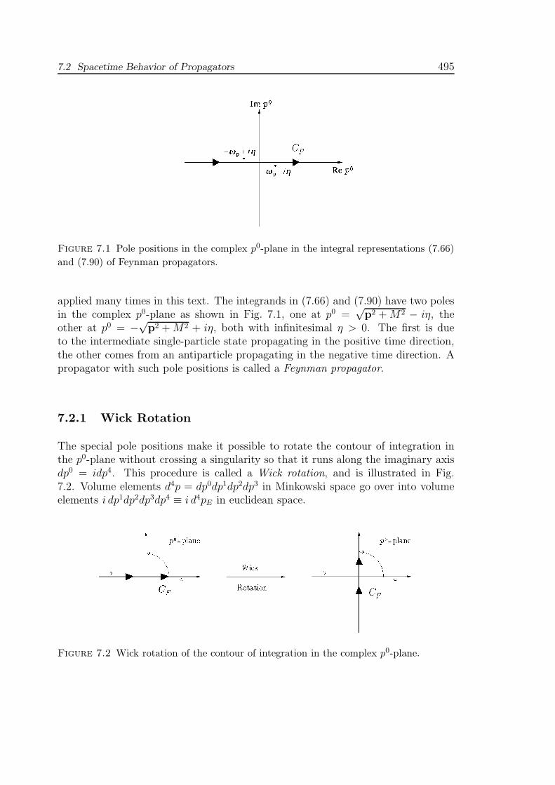
Figure 7.1 Pole positions in the complex p0-plane in the integral representations (7.66)

and (7.90) of Feynman propagators.

applied many times in this text. The integrands in (7.66) and (7.90) have two polesin the complex p0-plane as shown in Fig. 7.1, one at p0 =

√p2 +M2 − iη, the

other at p0 = −√p2 +M2 + iη, both with infinitesimal η > 0. The first is due

to the intermediate single-particle state propagating in the positive time direction,the other comes from an antiparticle propagating in the negative time direction. Apropagator with such pole positions is called a Feynman propagator.

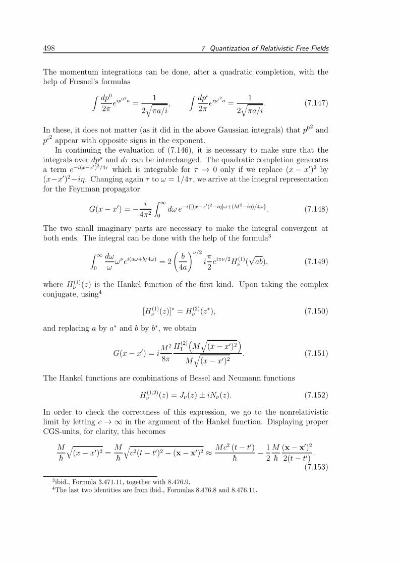
7.2.1 Wick Rotation

The special pole positions make it possible to rotate the contour of integration inthe p0-plane without crossing a singularity so that it runs along the imaginary axisdp0 = idp4. This procedure is called a Wick rotation, and is illustrated in Fig.7.2. Volume elements d4p = dp0dp1dp2dp3 in Minkowski space go over into volumeelements i dp1dp2dp3dp4 ≡ i d4pE in euclidean space.

Figure 7.2 Wick rotation of the contour of integration in the complex p0-plane.


By this procedure, the integral representations (7.66) and (7.90) for the propagatorbecome

G(x− x′) =∫

d4pE(2π)4

1

p2E +M2e−ipE(x−x′)E , (7.134)

where pµE is the four-momentum

pµE = (p1, p2, p3, p4 = −ip0), (7.135)

and p2E the square of the momentum pµE calculated in the euclidean metric, i.e.,p2E ≡ p1

2+ p2

2+ p3

2+ p4

2. The vector xµE is the corresponding euclidean spacetime

vectorxµE = (x1, x2, x3, x4 = −ix0), (7.136)

so that px = −pExE . With p2E+M2 being strictly positive, the integral (7.134) is now

well-defined. Moreover, the denominator possesses a simple integral representationin the form of an auxiliary integral over an auxiliary parameter τ which, as we shallsee later, plays the role of the proper time of the particle orbits:

1

p2E +M2=∫ ∞

0dτe−τ(p

2E+M2). (7.137)

Since this way of reexpressing denominators in propagators is extremely useful inquantum field theory, it is referred to, after its author, as Schwinger’s proper-time

formalism [2]. The τ -integral has turned the integral over the denominator into aquadratic exponential function. The exponent can therefore be quadratically com-pleted:

eipE(x−x′)E−τp2E → e−(x−x

′)2E/4τ−p′2Eτ , (7.138)

with p′E = pE− i(x−x′)E/2τ . Since the measure of integration is translationally in-variant, and the integrand has become symmetric under four-dimensional rotations,we can replace

∫

d4pE =∫

d4p′E = π2∫ ∞

0dp′E

2 p′E2, (7.139)

and integrate out the four-momentum p′E, yielding

G(x− x′) =1

16π2

∫ ∞

0

dτ

τ 2e−(x−x

′)2E/4τ−M2τ . (7.140)

The integral is a superposition of nonrelativistic propagators of the type (2.433),with Boltzmann-like weights e−M

2τ , and an additional weight factor τ−2 which maybe viewed as the effect of an entropy factor eS = e−2 log τ . This representation has aninteresting statistical interpretation. After deriving Eq. (2.433) for a nonrelativisticpropagator at imaginary times, we observed that this looks like the probability fora random walk of a fixed length proportional to hβ to go from x to x′ in three


dimensions. Here we see that the relativistic propagator looks like a random walk ofarbitrary length in four dimensions, with a length distribution ruled mainly by theabove Boltzmann factor. This leads to the possibility of describing, by relativisticquantum field theory, ensembles of random lines of arbitrary length. Such linesappear in many physical systems in the form of vortex lines and defect lines [6, 8, 18].

By changing the variable of integration from τ to ω = 1/4τ , this becomes

G(x− x′) =1

4π2

∫ ∞

0dω e−(x−x

′)2Eω−M2/4ω. (7.141)

Now we use the integral formula

∫ ∞

0

dω

ωωνe−aω−b/4ω = 2

(

b

4a

)ν/2

Kν(√ab), (7.142)

where Kν(z) is the modified Bessel function,2 to find

G(x− x′) =M2

4π2

K1

(

M√

(x− x′)2E

)

M√

(x− x′)2E. (7.143)

The D-dimensional generalization of this is calculated in the same way. Equation(7.140) becomes

G(x− x′) =1

(4π)D/2

∫ ∞

0

dτ

τD/2e−(x−x

′)2E/4τ−M2τ , (7.144)

yielding, via (7.142),

G(x− x′) =∫

dDq

(2π)D1

q2E +M2eiq(x−x

′)

=1

(2π)D/2

M√

(x− x′)2E

D/2−1

KD/2−1

(

M√

(x− x′)2E

)

. (7.145)

7.2.2 Feynman Propagator in Minkowski Space

Let us now do the calculation in Minkowski space. There the proper-time represen-tation of the propagators (7.66) and (7.90) reads

G(x−x′) =∫

d4p

(2π)4i


′) = i∫ ∞

0dτ∫

d4p

(2π)4e−i[p(x−x

′)−τ(p2−M2+iη)].

(7.146)

2I.S. Gradshteyn and I.M. Ryzhik, op. cit., Formula 3.471.9.


The momentum integrations can be done, after a quadratic completion, with thehelp of Fresnel’s formulas

∫

dp0

2πeip

02a =1

2√

πa/i,

∫

dpi

2πeip

i2a =1

2√

πa/i. (7.147)

In these, it does not matter (as it did in the above Gaussian integrals) that p02and

pi2appear with opposite signs in the exponent.In continuing the evaluation of (7.146), it is necessary to make sure that the

integrals over dpµ and dτ can be interchanged. The quadratic completion generatesa term e−i(x−x

′)2/4τ which is integrable for τ → 0 only if we replace (x − x′)2 by(x−x′)2−iη. Changing again τ to ω = 1/4τ , we arrive at the integral representationfor the Feynman propagator

G(x− x′) = − i

4π2

∫ ∞

0dω e−i[(x−x

′)2−iη]ω+(M2−iη)/4ω. (7.148)

The two small imaginary parts are necessary to make the integral convergent atboth ends. The integral can be done with the help of the formula3

∫ ∞

0

dω

ωωνei(aω+b/4ω) = 2

(

b

4a

)ν/2

iπ

2eiπν/2H(1)

ν (√ab), (7.149)

where H(1)ν (z) is the Hankel function of the first kind. Upon taking the complex

conjugate, using4

[H(1)ν (z)]∗ = H(2)

ν (z∗), (7.150)

and replacing a by a∗ and b by b∗, we obtain

G(x− x′) = iM2

8π

H(2)1

(

M√

(x− x′)2)

M√

(x− x′)2. (7.151)

The Hankel functions are combinations of Bessel and Neumann functions

H(1,2)ν (z) = Jν(z)± iNν(z). (7.152)

In order to check the correctness of this expression, we go to the nonrelativisticlimit by letting c → ∞ in the argument of the Hankel function. Displaying properCGS-units, for clarity, this becomes

M

h

√

(x− x′)2 =M

h

√

c2(t− t′)2 − (x− x′)2 ≈ Mc2 (t− t′)

h− 1

2

M

h

(x− x′)2

2(t− t′).

(7.153)

3ibid., Formula 3.471.11, together with 8.476.9.4The last two identities are from ibid., Formulas 8.476.8 and 8.476.11.


For large arguments, the Hankel functions behave like

H(1,2)ν (z) ≈ 2

πze±i(z−νπ/2−π/2), (7.154)

so that (7.151) becomes, for t > t′, and taking into account the nonrelativistic limit(4.156) of the fields,

G(x− x′)c→∞−−−→ 1

2M

1√

2πih(t− t′)/M3 exp

[

i

h

M

2t(x− x′)2

]

, (7.155)

in agreement with the nonrelativistic propagator (2.241).

In the spacelike regime (x − x′)2 < 0, we continue√

(x− x′)2 analytically to

−i√

−(x− x′)2, and H(2)1 (z) = H

(1)1 (−z) together with the relation5

πi

2

H(1)ν (iz)

(iz)ν=Kν(z)

zν, (7.156)

to rewrite (7.151) as

G(x− x′) =M

4π2

K1

(

M√

−(x− x′)2)

M√

−(x− x′)2, (x− x′)2 < 0, (7.157)

in agreement with (7.143).It is instructive to study the massless limit M → 0, in which the asymptotic

behavior6 K(z) → 1/z leads to

G(x− x′) → 1

4π2

1

(x− x′)2E. (7.158)

To continue this back to Minkowski space where (x−x′)2E = −(x−x′)2, it is necessaryto remember the small negative imaginary part on x2 which was necessary to makethe τ -integral (7.148) converge. The correct massless Green function in Minkowskispace is therefore

G(x− x′) = − 1

4π2

1

(x− x′)2 − iη. (7.159)

The same result is obtained from theM → 0 -limit of the Minkowski space expression(7.151), using the limiting property7

H(1)ν (z) ≈ −H(2)

ν (z) ≈ − i

πΓ(ν)

1

(z/2)ν. (7.160)

5ibid., Formula 8.407.1.6M. Abramowitz and I. Stegun, Handbook of Mathematical Functions , Dover, New York, 1965,

Formula 9.6.9.7ibid., Formula 9.1.9.


7.2.3 Retarded and Advanced Propagators

Let us contrast the spacetime behavior of the Feynman propagators (7.151) and(7.159) with that of the retarded propagator of classical electrodynamics. A retardedpropagator is defined for an arbitrary interacting field φ(x) by the expectation value

GR(x− x′) ≡ Θ(x0 − x′0)〈0|[φ(x), φ(x′)]|0〉. (7.161)

In general, one defines a commutator function C(x− x′) by

C(x− x′) ≡ 〈0|[φ(x), φ(x′)]|0〉, (7.162)

leading toGR(x− x′) = Θ(x0 − x′0)C(x− x′). (7.163)

For a free field φ(x), the commutator is a c-number, so that the vacuum expectationvalues can be omitted, and C(x − x′) is given by (7.56), leading to a retardedpropagator

GR(x− x′) = Θ(x0 − x′0)[G(+)(x− x′)−G(−)(x− x′)]. (7.164)

The Heaviside function in front of the commutator function C(x − x′) ensuresthe causality of this propagator. It also has the effect of turning C(x − x′), whichsolves the homogenous Klein-Gordon equation, into a solution of the inhomogenous

equation. In fact, by comparing (7.164) with (7.62) and using the Fourier repre-sentations (7.63) of the Heaviside functions, we find, for the retarded propagator, arepresentation very similar to that of the Feynman propagator in (7.64), except fora reversed iη-term in the negative-energy pole:

GR(x− x′)=∫

dE

2π

d3p

(2π)31

2p0

(

i

E − p0 + iη− i

E + p0 + iη

)

e−iE(x0−x′0)+ip(x−x′).(7.165)

By combining the denominators we now obtain, instead of (7.65),

∫

dE

2π

d3p

(2π)3i

(E + iη)2 − p2 −M2e−iE(x0−x′0)+ip(x−x

′), (7.166)

which may be written as an off-shell integral of the type (7.66):

GR(x− x′) =∫

d4p

(2π)4i

p2+ −M2 + iηe−ip(x−x

′), (7.167)

where the subscript of p+ indicates that a small iη-term has been added to p0.Note the difference in the Fourier representation with respect to that of the

commutator function in (7.59). Due to the absence of a Heaviside function, thecommutator function solves the homogenous Klein-Gordon equation.

It is important to realize that the retarded Green function could be derived froma time-ordered expectation value of second-quantized field operators if we assume


that the Fourier components with the negative frequencies are associated with an-nihilation operators d−p rather than creation operators b†p of antiparticles. Thenthe propagator would vanish for x0 < x′0, implying both poles in the p0-plane to liebelow the real energy axis.

For symmetry reasons, one also introduces an advanced propagator

GA(x− x′) ≡ Θ(x′0 − x0)〈0|[φ(x), φ(x′)]|0〉. (7.168)

It has the same Fourier representation as GR(x− x′), except that the poles lie bothabove the real axis:

GA(x− x′) =∫

d4p

(2π)4i

p2− −M2e−ip(x−x

′). (7.169)

There will be an application of this Green function in Subsec. 12.12.1.Let us calculate the spacetime behavior of the retarded propagator. We shall

first look at the massless case familiar from classical electrodynamics. For M = 0,the integral representation (7.167) reads

GR(x− x′) ≡∫ d4p

(2π)4e−ip(x−x

′) i

p2+, (7.170)

but with the poles in the p0-plane at

p0 = p0 = ±ωp = ±|p|, (7.171)

both sitting below the real axis. This is indicated by writing p2+ in the denominatorrather than p2, the plus sign indicating an infinitesimal +iη added to p0.

In the Feynman case, the p0-integral is evaluated with the decomposition (7.64)and the integral representation (7.63) of the Heaviside function as follows:

∫

dp0

2πe−ip

0(x0−x′0) i

2ωp

(

1

p0 − ωp + iη− 1

p0 + ωp − iη

)

(7.172)

=1

2ωp

[Θ(x0 − x′0)e−iωp(x0−x′0) +Θ(x′0 − x0)eiωp(x0−x′0)] =1

2ωp

e−iωp|x0−x′0|.

In contrast, the retarded expression reads

∫

dp0

2πe−ip

0(x0−x′0) i

2ωp

(

1

p0 − ωp + iη− 1

p0 + ωp + iη

)

= Θ(x0 − x′0)1

2ωp

[e−iωp(x0−x′0) − eiωp(x0−x′0)]. (7.173)

Thus we may write

G(x− x′) =∫ d3p

(2π)32ωp

eip(x−x′)e−iωp|x0−x′0|, (7.174)

GR(x− x′) = Θ(x0 − x′0)∫

d3p

(2π)32ωp

eip(x−x′)[e−iωp(x0−x′0) − eiωp(x0−x′0)]. (7.175)


In the retarded expression we recognize, behind the Heaviside prefactor Θ(x0−x′0),the massless limit of the commutator function C(x, x′) = C(x−x′) of Eq. (7.57), inaccordance with the general relation (7.163).

The angular parts of the spatial part of the Fourier integral

∫ d3p

(2π)3eip(x−x

′) (7.176)

are the same in both cases, producing an integral over |p|:1

2πR

∫ ∞

0

d|p|π

|p| sin (|p|R), (7.177)

where R ≡ |x−x′|. The Feynman propagator has therefore the integral representa-tion

G(x− x′) =1

4πR

∫ ∞

0

d|p|π

|p|ωp

sin (|p||R) e−iωp|x0−x′0|. (7.178)

In the massless case where ωp = |p|, we can easily perform the |p|-integration andrecover the previous result (7.159).

To calculate the retarded propagator GR(x − x′) = Θ(x0 − x′0)C(x − x′) inspacetime, we may focus our attention upon the commutator function, whose inte-gral representation is now

C(x− x′) =1

4πR

∫ ∞

0

dp

π

p

ωp

sin (pR) [e−iωp(x0−x′0)−eiωp(x0−x′0)]. (7.179)

In the massless case where ωp = p, we decompose the trigonometric function intoexponentials, and obtain

C(x− x′) = −i 1

4πR

∫ ∞

−∞

dω

2π

e−iω[(x0−x′0)−R]− e−iω[(x

0−x′0)+R]

, (7.180)

which is equal to

C(x− x′) = −i 1

4πR

[

δ(x0 − x′0 − R)− δ(x0 − x′0 +R)]

. (7.181)

It is instructive to verify in this expression the canonical equal-time commutationproperties (7.58). For this we multiply C(x) by a test function f(r) and calculate,with r = |x|,

∫

d3x C(x)f(r) = −i∫

dr r21

r

[

δ(x0 − r)− δ(x0 + r)]

. (7.182)

Since δ(x0 − r) − δ(x0 + r) = −(d/dr)[δ′(x0 − r) + δ′(x0 + r)], we can perform apartial integration and find

−i∫

dr[

δ(x0 − r) + δ(x0 + r)]

[rf(r)]′ = −i ddx0

[|x0|f(|x0|)]. (7.183)


At x0 = 0, this is equal to −if(0) at x0 = 0, as it should.Using the property of the δ-function (7.61) in spacetime

δ(x02 − r2) =1

2r[δ(x0 − r) + δ(x0 + r)], (7.184)

we can also write the commutator function as

C(x− x′) = −iǫ(x0 − x′0)1

2πδ((x− x′)2), (7.185)

where ǫ(x0 − x′0) is defined by

ǫ(x0 − x′0) ≡ Θ(x0 − x′0)−Θ(−x0 + x′0), (7.186)

which changes the sign of the second term in the decomposition (7.184) of δ((x−x′)2)to the form required in (7.184).

Note that in the form (7.185), the canonical properties (7.58) of the commutatorfunction cannot directly be verified, since ǫ(x0 − x′0) = 2δ(x0 − x′0) is too singularto be evaluated at equal times. In fact, products of distributions are in generalundefined, and their use is forbidden in mathematics.8 We must read ǫ(x0)δ(x2) asthe difference of distributions

ǫ(x0)δ(x2) ≡ 1

2r[δ(x0 − r)− δ(x0 + r)] (7.187)

to deduce its consequences. Then with (7.185), the retarded propagator (7.163)becomes

GR(x− x′) = −iΘ(x0 − x′0)1

4πR

[

δ(x0 − x′0 −R)− δ(x0 − x′0 +R)]

= −iΘ(x0 − x′0)1

2πδ((x− x′)2). (7.188)

The Heaviside function allows only positive x0−x′0, so that only the first δ-functionin (7.188) contributes, and we obtain the well-known expression of classical electro-dynamics:

GR(x− x′) = −iΘ(x0 − x′0)1

4πRδ(x0 − x′0 − R). (7.189)

This propagator exists only for a causal time order x0 > x′0, for which it is equal tothe Coulomb potential between points which can be connected by a light signal.

The retarded propagator GR(x, x′) describes the massless scalar field φ(x) caused

by a local spacetime event iδ(4)(x′). For a general source j(x′), it serves to solve theinhomogeneous field equation

−∂2φ(x) = j(x) (7.190)

8An extension of the theory of distributions that includes also their products is developed inthe textbook H. Kleinert, Path Integrals in Quantum Mechanics, Statistics, Polymer Physics, and

Financial Markets , World Scientific, Singapore 2009 (klnrt.de/b5).


by superposition:

φ(x) = −i∫

d4xGR(x, x′)j(x′). (7.191)

Inserting (7.189), and separating the integral into time and space parts, the time x′0can be integrated out and the result becomes

φ(x, t) = −∫

d3x′1

4π|x− x′|j(x′, tR), (7.192)

where

tR = t− |x− x′| (7.193)

is the time at which the source has emitted the field which arrives at the spacetimepoint x. Relation (7.192) is the basis for the derivation of the Lienard-Wiechert

potential, which is recapitulated in Appendix 7B.

7.2.4 Comparison of Singular Functions

Let us compare the spacetime behavior (7.188), (7.189) of the retarded propagatorwith that of the massless Feynman propagator. The denominator in (7.159) can bedecomposed into partial fractions, and we find a form very close to (7.188):

G(x− x′) = − 1

8π2R

[

1

|x0 − x′0| − R− iη− 1

|x0 − x′0|+R − iη

]

. (7.194)

Feynman has found it useful to denote the function 1/(t− iη) by iπδ+(t). This hasa Fourier representation which differs from that of a Dirac δ-function by containingonly positive frequencies:

δ+(t) ≡∫ ∞

0

dω

πe−iω(t−iη). (7.195)

The integral converges at large frequencies only due to the −iη -term, yielding

δ+(t) = −1

π

i

t− iη. (7.196)

The pole term can be decomposed as9

1

t− iη=

iη

t2 + η2+

t

t2 + η2= iπδ(t) +

Pt. (7.197)

Recall that the decomposition concerns distributions which make sense only if theyare used inside integrals as multipliers of smooth functions. The symbol P in the

9This is often referred to as Sochocki’s formula. It is the beginning of an expansion in powersof η > 0: 1/(x± iη) = P/x∓ iπδ(x) + η [πδ′(x) ± idxP/x] +O(η2).


second term means that the integral has to be calculated with the principal-value

prescription.10 For the function δ+(t), the decomposition reads

δ+(t) = δ(t)− i

π

Pt. (7.198)

An important property of this function is that it satisfies a relation like δ(t) in(7.184):

δ+(t2 − r2) =

1

2r[δ+(t− r)− δ+(t + r)]. (7.199)

Below we shall also need the complex conjugate of the function δ+(t):

δ−(t) =1

π

i

t + iη= [δ+(t)]

∗. (7.200)

From (7.197) we see that the two functions are related by

δ+(t) + δ−(t) = 2δ(t). (7.201)

Because of (7.199), the Feynman propagator (7.194) can be rewritten as

G(x− x′)=− 1

8π2R

[

δ+(|x0 − x′0| −R)− δ+(|x0 − x′0|+R)]

=− i

4πδ+((x− x′)2).

(7.202)

These expressions look very similar to those for the retarded propagator inEqs. (7.188) and (7.189).

It is instructive to see what becomes of the δ+-function in Feynman propagatorsin the presence of a particle mass. According to (7.148), a mass term modifies theintegrand in

δ+((x− x′)2) =∫ ∞

0

dω

πe−iω(x−x

′)2 , (7.203)

(in which we omit the −iη term, for brevity) from e−iω(x−x′)2 to e−iω(x−x

′)2−iM2/4ω.We may therefore define a massive version of δ+((x− x′)2) by

δM+ ((x− x′)2) =∫ ∞

0

dω

πe−iω(x−x

′)2−iM2/2ω = −M2

2

H(2)1

(

M√

(x− x′)2)

M√

(x− x′)2. (7.204)

A similar generalization of the function δ((x − x′)2) in (7.185) to δM((x − x′)2)may be found by evaluating the commutator function C(x − x′) in Eq. (7.185) ata nonzero mass M . Its Fourier representation was given in Eq. (7.179) and may bewritten as

C(x− x′) = − i

2π2

∫ ∞

0

d|p| |p|2√

|p|2 +M2

sin (|p|R)|p|R sin[p0(x0 − x′0)]. (7.205)

10Due to the entirely different context, no confusion is possible with the second-quantized parityoperator P introduced in (7.96).


This can be expressed as a derivative

C(x− x′) = − i

4π

1

r

d

drF (r, x0 − x′0) (7.206)

of the function

F (r, t) =1

π

∫ ∞

−∞

dp√p2 +M2

cos(pR) sin√

p2 +M2t. (7.207)

The integral yields [2]:

F (r, t) =

J0(M√t2 − r2) for t > r,

0 for t ∈ (−r, r),−J0(M

√t2 − r2) for t < −r,

(7.208)

where Jµ(z) are Bessel functions. By carrying out the differentiation in (7.206),using J ′0(z) = −J1(z), we may write

C(x− x′) = −iǫ(x0 − x′0)δM((x− x′)2), (7.209)

with

δM(x2) = δ(x2)−Θ(x2)M2

2

J1(M√x2)

M√x2

. (7.210)

The function Θ(x2) enforces the vanishing of the commutator at spacelike distances,a necessity for the causality of the theory. Using (7.210), we can write the retardedpropagator GR(x− x′) = Θ(x0 − x′0)C(x− x′) as

GR(x− x′) = −iΘ(x0 − x′0)1

2πδM((x− x′)2). (7.211)

In the massless limit, the second term in (7.210) disappears since J1(z) ≈ z for smallz, and (7.211) reduces to (7.188).

Summarizing, we may list the Fourier transforms of the various propagators asfollows:

Feynman propagator :i

p2 −M2 + iη= πδ−(p

2 −M2) = πδ−(p02 − ω2

p);

=π

2ωp

[δ−(p0 − ωp) + δ+(p

0 + ωp)];

retarded propagator :i

p2+ −M2=

π

2ωp

[δ−(p0 − ωp)− δ−(p

0 + ωp)];

advanced propagator :i

p2− −M2= − π

2ωp

[δ+(p0 − ωp)− δ+(p

0 + ωp)];

commutator : 2πǫ(p0)δ(p2 −M2) = 2πǫ(p0)δ(p02 − ω2p)

=π

ωp

[δ−(p0 − ωp)− δ+(p

0 + ωp)].

(7.212)


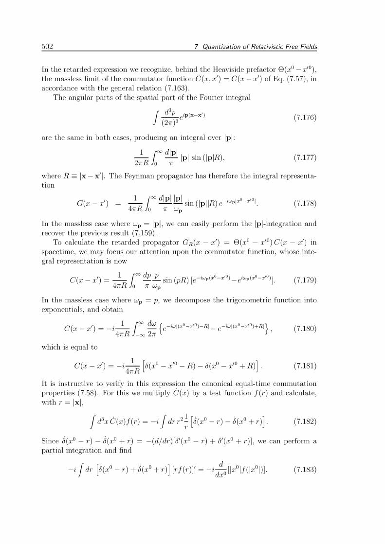
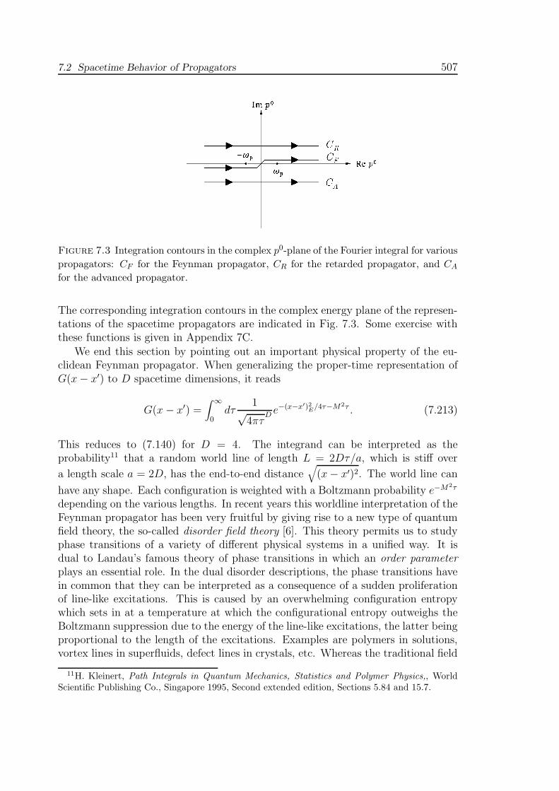
Figure 7.3 Integration contours in the complex p0-plane of the Fourier integral for various

propagators: CF for the Feynman propagator, CR for the retarded propagator, and CAfor the advanced propagator.

The corresponding integration contours in the complex energy plane of the represen-tations of the spacetime propagators are indicated in Fig. 7.3. Some exercise withthese functions is given in Appendix 7C.

We end this section by pointing out an important physical property of the eu-clidean Feynman propagator. When generalizing the proper-time representation ofG(x− x′) to D spacetime dimensions, it reads

G(x− x′) =∫ ∞

0dτ

1√4πτ

D e−(x−x′)2E/4τ−M

2τ . (7.213)

This reduces to (7.140) for D = 4. The integrand can be interpreted as theprobability11 that a random world line of length L = 2Dτ/a, which is stiff over

a length scale a = 2D, has the end-to-end distance√

(x− x′)2. The world line can

have any shape. Each configuration is weighted with a Boltzmann probability e−M2τ

depending on the various lengths. In recent years this worldline interpretation of theFeynman propagator has been very fruitful by giving rise to a new type of quantumfield theory, the so-called disorder field theory [6]. This theory permits us to studyphase transitions of a variety of different physical systems in a unified way. It isdual to Landau’s famous theory of phase transitions in which an order parameter

plays an essential role. In the dual disorder descriptions, the phase transitions havein common that they can be interpreted as a consequence of a sudden proliferationof line-like excitations. This is caused by an overwhelming configuration entropywhich sets in at a temperature at which the configurational entropy outweighs theBoltzmann suppression due to the energy of the line-like excitations, the latter beingproportional to the length of the excitations. Examples are polymers in solutions,vortex lines in superfluids, defect lines in crystals, etc. Whereas the traditional field

11H. Kleinert, Path Integrals in Quantum Mechanics, Statistics and Polymer Physics,, WorldScientific Publishing Co., Singapore 1995, Second extended edition, Sections 5.84 and 15.7.


theoretic description of phase transitions due to Landau is based on the introductionof an order parameter and its spacetime version, an order field, the new descriptionis based on a disorder field describing random fluctuations of line-like excitations.As a result of this different way of looking at phase transitions one obtains a fieldtheoretic formulation of the statistical mechanics of line ensembles, that yields asimple explanation of the phase transitions in superfluids and solids.

7.3 Collapse of Relativistic Wave Function

As earlier in the nonrelativistic discussion on p. 120, a four-field Green function canbe used to illustrate the relativistic version of the notorious phenomenon of thecollapse of the wave function in quantum mechanics [5]. If we create a particle atsome spacetime point x′ = (x′0,x

′), we generate a Klein-Gordon wave function thatcovers the forward light cone of this point x′. If we annihilate the particle at somedifferent spactime point x′ = (x′0,x

′), the wave function disappears from spacetime.Let us see how this happens about in the quantum field formalism. The creationand later annihilation process give rise to a Klein-Gordon field

〈ϕ(x)ϕ†(x′)〉 =∑

p

1

2V ωp

e−ip(x−x′). (7.214)

If we measure the particle densityat a spacetime x′′ point that lies only slightly laterthan the later spacetime point t by inserting the current operator (7.128) in theabove Green function, we find

G(x′′, x, x′) = 〈0|ρ(x′′)ϕ(x)ϕ†(x′)|0〉= −〈0|iϕ†(x′′)

↔

∂0ϕ(x′′)ϕ(x)ϕ†(x′)|0〉. (7.215)

The second and the fourth field operators yield a Green function Θ(x′′0−x′0)G(x′′−x′).This is multiplied by the Green function of the first and the third field operatorswhich is Θ(x− x′′)G(x′′ − x′), und is thus equal to zero since x

′′

0 > x0. Thus provesthat by the time x′0 > x0, the wave function created at the initial spacetime pointx′ has completely collapsed. More interesting is the situation if we perform ananalogous study for a state |ϕ(x′1)ϕ(x′2)〉 that contains two particles. Here we lookat the Green function

G(x′′, x1, x′1, x2, x

′2) = 〈0|ρ(x′′)ϕ(x1)ϕ(x2)ϕ†(x′1)ϕ†(x′2)|0〉

= −〈0|iϕ†(x′′)↔

∂0ϕ(x′′)ϕ(x1)ϕ(x2)ϕ

†(x′1)ϕ†(x′2)|0〉.(7.216)

Depending on the various positions of x′′ with respect to x1 and x2, we can ob-serve the consequences of putting counter for one particle of the two-particle wavefunction, i.e., from which we learn of the collapse of a one-particle content of thetwo-particle wave function.12

12K.E. Hellwig and K. Kraus, Phys. Rev. D 1, 566 (1970).

7.4 Free Dirac Field 509

7.4 Free Dirac Field

We now turn to the quantization of the Dirac field obeying the field equation (4.500):

(iγµ∂µ −M)ψ(x) = 0. (7.217)

Their plane-wave solutions were given in Subsec. 4.13.1, and just as in the case ofa scalar field, we shall introduce creation and annihilation operators for particlesassociated with these solutions.

The classical Lagrangian density is [recall (4.501)]:

L(x) = ψ(x)iγµ∂µψ(x)−Mψ(x)ψ(x). (7.218)


The canonical momentum of the ψ(x) field is

π(x) =∂L(x)

∂[∂0ψ(x)]= iψ(x)γ0 = iψ†(x). (7.219)

Up to the factor i, this is equal to the complex-conjugate field ψ†, as in the non-relativistic equation (7.5.1). Note that the field ψ has no conjugate momentum,since

∂L(x)∂[∂0ψ(x)]

= 0. (7.220)

This zero is a mere artifact of the use of complex field variables. It is unrelatedto a more severe problem in Section 7.5.1, where the canonical momentum of acomponent of the real electromagnetic vector field vanishes as a consequence ofgauge invariance.

If ψ(x, t) were a Bose field, its canonical commutation rule would read

[ψ(x, t), ψ†(x′, t)] = δ(3)(x− x′). (7.221)

However, since electrons must obey Fermi statistics to produce the periodic systemof elements, the fields have to satisfy anticommutation rules

ψ(x, t), ψ†(x′, t)

= δ(3)(x− x′). (7.222)

Recall that in the nonrelativistic case, this modification of the commutation ruleswas dictated by the Pauli principle and the implied antisymmetric electronic wavefunctions. To ensure this, the relativistic theory can be correctly quantized only

by anticommutation rules. Commutation rules (7.221) are incompatible either withmicrocausality or the positivity of the energy. This will be shown in Section 7.10.

We now expand the field ψ(x) into the complete set of classical plane-wavesolutions (4.662). In a large but finite volume V , the expansion reads

ψ(x) =∑

p,s3

[

fp s3(x)ap,s3 + f cp s3(x)b†p,s3

]

, (7.223)


or more explicitly:

ψ(x) =∑

p,s3

1√

V p0/M

[

e−ipxu(p, s3)ap,s3 + eipxv(p, s3)b†p,s3

]

. (7.224)

As in the scalar equation (7.12), we have associated the expansion coefficients of theplane waves eipx with a creation operator b†p,s3 rather than an annihilation operator

d†−p,−s3. For reasons similar to those explained after Eqs. (7.75) and (7.87), the signis reversed in both p and s3.

Expansion (7.224) is inverted and solved for ap,s3 and b†p,s3 by applying theorthogonality relations (4.665) for the bispinors u(p, s3) and v(−p, s3) to the spatialFourier transform∫

d3x e−ipxψ(x) =∑

p,s3

√V

√

p0/M

[

e−ip0x0u(p, s3)ap,s3 + eip

0x0v(−p, s3)b†−p,s3

]

. (7.225)

The results are

ap,s3 = eip0x0 1

√

V p0/Mu†(p, s3)

∫

d3x e−ipxψ(x),

b†p,s3 = e−ip0x0 1√

V p0/Mv†(p, s3)

∫

d3x eipxψ(x), (7.226)

these being the analogs of the scalar equations (7.76). The same results can, ofcourse, be obtained from (7.223) with the help of the scalar products (4.664), interms of which Eqs. (7.226) are simply

ap,s3 = (fp s3, ψ)t, b†p,s3 = (f cp s3 , ψ)t, (7.227)

as in the scalar equations (7.19).From (7.226) we derive that all anticommutators between ap,s3, a

†p′,s′3

, bp,s3, b†p′,s′3

vanish, except for

ap,s3, a†p′,s′3

=

√

M

p0M

p0′u†(p, s3)u(p

′, s′3)δp,p′ = δp,p′δs3,s′3, (7.228)

bp,s3, b†p′,s′3

=

√

M

p0M

p0′v†(p, s3)v(p, s3)δp,p′ = δp,p′δs3,s′3. (7.229)

The single-particle states|p, s3〉 = a†p,s3|0〉 (7.230)

have the wave functions

〈0|ψ(x)|p, s3〉 =1

√

V p0/Me−ipxu(p, s3) = fp,s3(x)

〈p, s3|ψ(x)|0〉 =1

√

V p0/Meipxu(p, s3) = fp,s3(x). (7.231)


The similar antiparticle states

|p, s3〉 = b†p,s3|0〉, (7.232)

have the matrix elements

〈ps3|ψ(x)|0〉 =1

√

V p0/Meipxv(p, s3) = fcp,s3(x),

〈0|ψ(x)|p, s3〉 =1

√

V p0/Me−ipxu(p, s3) = fcp,s3(x). (7.233)

As in the scalar field expansion (7.75), the negative-frequency solution v(p, s3)eipx

of the Dirac equation is associated with a creation operator b†p,s3 of an antiparticlerather than a second annihilation operator d−p,−s3. This ensures that the antiparticlestate |ps3〉 has the same exponential form e−ipx as that of |p, s3〉, both exhibiting thesame time dependence e−ip

0t with a positive energy p0 = ωp. The other assignmentwould have given a negative energy.

In an infinite volume, a more convenient field expansion makes use of the plane-wave solutions (4.666). It uses covariant creation and annihilation operators as in(7.16) to expand:

ψ(x) =∫

d3p

(2π)3p0/M

∑

s3

[

e−ipxu(p, s3)ap,s3 + eipxv(p, s3)b†p,s3

]

. (7.234)

The commutation rules between ap,s3, a†p,s3, bp,s3, and b†p,s3 are the same as in (7.228)

and (7.229), but with a replacement of the Kronecker symbols by their invariantcontinuum version similar to (7.20):

δp,p′ → p0

M-δ(3)(p− p′) =

p0

M(2πh)D -δ

(3)(p− p′). (7.235)

Note that this fermionic normalization is different from the bosonic one in (7.20),where the factor in front of the -δ-function was 2p0. This is a standard conventionthroughout the literature.

In an infinite volume, we may again introduce single-particle states

|p, s3) = a†p,s3|0), |p, s3) = b†p,s3|0), (7.236)

with the vacuum |0) defined by ap,s3|0) = 0 and bp,s3|0) = 0. These states willsatisfy the orthogonality relations

(p′, s′3|p, s3) =p0

M-δ(3)(p′ − p)δs′3,s3, (p′, s′3|p, s3) =

p0

M-δ(3)(p′ − p)δs′3,s3,

(7.237)in accordance with the replacement (7.235) [and in contrast to the normalization(7.27) for scalar particles]. They have the wave functions

(0|ψ(x)|p, s3) = e−ipxu(p, s3) = fp,s3(x), (p, s3|ψ(x)|0) = eipxu(p, s3) = fp,s3(x).

(p, s3|ψ(x)|0)= eipxv(p, s3) = fcp,s3(x), 〈0|ψ(x)|p, s3〉 = e−ipxv(p, s3) = fcp,s3(x).

(7.238)


We end this section by stating also the explicit form of the quantized field ofmassless left-handed neutrinos and their antiparticles, the right-handed antineutri-nos:

ψν(x) =1− γ5

2ψ(x) =

∑

p

1√2V p0

[

e−ipxuL(p)ap,− 12+ eipxvR(p)b

†

p, 12

]

, (7.239)

where the operators a†p,− 1

2

and b†p, 12

carry helicity labels ∓12, and p0 = |p|. The

massless helicity bispinors are those of Eqs. (4.726) and (4.727). Remember thenormalization (4.725):

u†L(p)uL(p) = 2p0, u†R(p)uR(p) = 2p0,

v†L(p)vL(p) = 2p0, v†R(p)vR(p) = 2p0, (7.240)

which is the reason for the factor 1/√2V p0 in the expansion (7.239) [as in the

expansions (7.12) and (7.75) for the scalar mesons].

7.4.2 Energy of Free Dirac Particles

We now turn to the energy of the free quantized Dirac field. The energy density isgiven by the Legendre transform of the Lagrangian density

H(x) = π(x)ψ(x)−L(x)= iψ†(x)ψ(x)− L(x)= ψ(x)iγi∂iψ(x) +Mψ(x)ψ(x). (7.241)

Inserting the expansion (7.224) and performing the spatial integral [recall the stepfrom (7.30) to (7.31)], the double sum over momenta reduces to a single sum, andwe obtain the second-quantized Hamilton operator

H =∑

p,s3,s′3

M

p0

[

a†p,s3ap,s′3u(p, s3)(γipi +M)u(p, s′3)

+ bp,s3b†p,s′3

v(p, s3)(−γipi +M)v(p, s′3)

+ a†p,s3b†−p,s′3

u(p, s3)(γipi +M)v(−p, s′3)e

2ip0t

+ b−p,s3ap,s′3 v(−p, s3)(γipi +M)u(p, s′3)e

2ip0t]

. (7.242)

We now use the Dirac equation, according to which

(γipi +M)u(p, s3) = γ0p0u(p, s3),

(−γipi +M)v(p, s3) = −γ0p0v(p, s3), (7.243)

and the orthogonality relations (4.696)–(4.699), and simplify (7.243) to

H =∑

p,s3

p0(

a†p,s3ap,s3 − bp,s3b†p,s3

)

. (7.244)


With the help of the anticommutation rule (7.229), this may be rewritten as

H =∑

p,s3

p0(

a†p,s3ap,s3 + b†p,s3bp,s3)

−∑

p,s3

p0. (7.245)

The total energy adds up all single-particle energies. In contrast to the second-quantized scalar field, the vacuum has now a negatively infinite energy due to thezero-point oscillations, as announced in the discussion of Eq. (7.37).

Note that if we had used here the annihilation operators of negative energy statesd−p,−s3 instead of the creation operators b†p,s3, then the energy would have read

H =∑

p,s3

p0(

a†p,s3ap,s3 − d†p,s3dp,s3)

, (7.246)

so that the particles created by d†p,s3 would again have had negative energies. Bygoing over from d−p,−s3 to b

†p,s3

, we have transformed missing negative energy statesinto states of antiparticles, thereby obtaining a positive sign for the energy of anantiparticle. This happens, however, at the expense of having a negatively infi-nite zero-point energy of the vacuum. This also explains why the spin orientations3 changes sign under the above replacement. A missing particle with spin downbehaves like a particle with spin up.

Actually, the above statements about the exchange dp,s3 → b†p,s3 are correct onlyas far as the sum of all momentum states and spin indices s3 in (7.246) is concerned.For a single state, we also have to consider the momentum operator and the spin.

The situation is the same as in the free-electron approximation to the electronsin a metal. At zero temperature, the electrons are in the ground state, forming aFermi sea in which all single-particle levels below a Fermi energy EF are occupied.If all energies are measured from that energy, all occupied levels have a negativeenergy, and the ground state has a large negative value. If an electron is kickedout from one of the negative-energy states, an electron-hole pair is observed, bothparticle and hole carrying a positive energy with respect to the undisturbed Fermiliquid. The hole appears with a positive charge relative to the Fermi sea.

Note also that unlike the Bose case, the exchange d−p,−s3 → b†p,s3 maintains thecorrect sign of canonical anticommutation rules (7.229). In fact, the negative sign ofthe term −d†p,s3dp,s3 in the Hamilton operator (7.246) is somewhat less devastatingthan in the Bose case. It can actually be avoided by a mere redefinition of thevacuum as the state in which all momenta are occupied by a d†p,s3 particle:

|0〉new =∏

p,s3

d†p,s3|0〉. (7.247)

This state has now the same negative infinite energy

E0 new ≡ new〈0|H|0〉new = −∑

p,s3

p0, (7.248)

found in the correct quantization. Counting from this ground state energy, allother states have positive energies, obtained either by adding a particle with the


operator a†p,s3 or by removing a particle with d−p,−s3. Of course, this descriptionis just a reflection of the fact that if creation and annihilation operators satisfyanticommutation rules −d†p,s3dp,s3 = dp,s3d

†p,s3−1, a reinterpretation of the operators

d−p,−s3 → b†p,s3 and d†−p,−s3 → bp,s3 makes the product dp,s3d

†p,s3 a positive operator.

For commutators, the same reinterpretation is impossible since −d†p,s3dp,s3 can haveany negative eigenvalue and it is impossible to introduce a new “zero level” thatwould make all energy differences positive!

It was the major discovery of Dirac that the annihilation of a negative-energyparticle may be viewed as a creation of a positive-energy particle with the samemass and spin, but with reversed directions of momentum and spin. Dirac calledit the antiparticle. When dealing with electrons, the antiparticle is a positron.Dirac imagined all negative energy states in the world as being filled, forming asea of negative energy states, just as the above-described Fermi sea in metals. Theannihilation of a negative-energy particle in the sea would create a hole which wouldappear to the observer as a particle of positive energy with the opposite charge.

As in the scalar case of Eqs. (7.32)–(7.36), it is often possible to simply dropthis infinite energy of the vacuum by introducing a normal product :H: . As before,the double dots mean: Order all operators such that all creators stand to the leftof all annihilators. But in contrast to the boson case, every transmutation of twoFermi operators, done to achieve the normal order, is now accompanied by a phasefactor −1.

7.4.3 Lorentz Transformation Properties of Particle States

The behavior of the bispinors u(p, s3) and v(p, s3) under Lorentz transformationsdetermines the behavior of the creation and annihilation operators of particles andantiparticles, and thus of the particle states created by them, in particular thesingle-particle states (7.230) and (7.232). Under a Lorentz transformation Λ, thefield operator ψ(x) transforms according to the law (4.521):

ψ(x)Λ−−−→ ψ′Λ(x) = D(Λ)ψ(Λ−1x) = e−i

12ωµνSµν

ψ(Λ−1x), (7.249)

On the right-hand side, we now insert the expansion (7.234), so that

D(Λ)ψ(Λ−1x) =∫

d3p

(2π)3p0/M

∑

s3,s′3

[

e−ip′xu(p′, s′3)Ws′3,s3

(p′,Λ, p) ap,s3

+ eip′xv(p′, s′3)W

∗s′3,s3

(p′,Λ, p) b†p,s3

]

,

where we have set p′ ≡ Λp, and used the fact that pΛ−1x = p′x. In order to derivethe transformation laws for the creation and annihilation operators, we rewrite thisexpansion in the same form as the original (7.234), expressing it now in terms ofprimed momenta and spins:

D(Λ)ψ(Λ−1x)=∫

d3p′

(2π)3p′0/M

∑

s3,s′3

[

e−ip′xu(p′, s′3)a

′p′,s′3

+ eip′xv(p′, s′3)b

′†p′,s′3

]

.(7.250)


Because of the Lorentz invariance of the integration measure in momentum spaceobserved in (4.184), we can replace in (7.250)

∫

d3p

(2π)3p0/M→∫

d3p

(2π)3p′0/M. (7.251)

Comparing now the coefficients, we find the transformation laws

ap′,s′3

Λ−−−→ a′p′,s′3=

1/2∑

s3=−1/2

Ws′3,s3(p′,Λ, p) ap,s3,

b†p′,s′3

Λ−−−→ b′†p′,s′3

=1/2∑

s3=−1/2

W ∗s′3,s3

(p′,Λ, p) b†p,s3. (7.252)

In contrast to the Lorentz transformations (7.249) of the field, the creation andannihilation operators are transformed unitarily under the Lorentz group. Theright-hand sides define a unitary representation of the Lorentz transformations Λ:

a′p′,s′3= U−1(Λ)ap′,s′3

U(Λ) =1/2∑

s3=−1/2

Ws′3,s3(p′,Λ, p) ap,s3,

b′†p′,s′3

= U−1(Λ)b†p′,s′3

U(Λ) =1/2∑

s3=−1/2

W ∗s′3,s3

(p′,Λ, p) b†p,s3, (7.253)

with similar relations for a†p,s3 and bp,s3. For the single-particle states (7.236), thisimplies the transformation laws:

U(Λ)|p, s3〉 = U(Λ)a†p,s3U−1(Λ)|0〉 =1/2∑

s′3=−1/2

|p′, s′3〉Ws′3,s3(p′,Λ, p),

U(Λ)|p, s3〉 = U(Λ)b†p,s3U−1(Λ)|0〉 =1/2∑

s′3=−1/2

|p′, s′3〉Ws′3,s3(p′,Λ, p), (7.254)

where we have used the Lorentz-invariance of the vacuum state

U(Λ)|0〉 = |0〉. (7.255)

We are now ready to understand the reason for introducing the matrix c in thebispinors v(p, s3) of Eq. (4.684), and thus the sign reversal of the spin orientation.In (4.742) we found that the canonical spin indices of v(p, s3) transformed underrotations by the complex-conjugate 2× 2 Wigner matrices with respect to those ofu(p, s3). This implies that the Wigner rotations mixing the spin components of theoperators ap,s3 and b†p,s3 are complex conjugate to each other. As a consequence,b†p,s3 transforms in the same way as a†p,s3, so that antiparticles behave in preciselythe same way as particles under Lorentz transformations.


For massless particles in the helicity representation, the creation and annihilationoperators transform under Lorentz transformations merely by a phase factor, asdiscussed at the end of Section 4.15.3.

Under translations by a four-vector aµ, the particle and antiparticle states|p, s3) = a†p,s3|0) and |p, s3) = b†p,s3|0) transform rather trivially. Since they havea definite momentum, they receive merely a phase factor eipa. This follows directlyfrom applying the transformation law (4.524) on the Dirac field operator:

ψ(x)−−−→ψ′(x) = ψ(x− a). (7.256)

Inserting the operator expansion (7.234) into the right-hand side, we see that thecreation and annihilation operators transform as follows:

ap,s3 −−−→ a′p,s3 = eipa ap,s3,

b†p,s3 −−−→ b′†p,s3 = e−ipa b†p,s3. (7.257)

These transformation laws define a unitary operator of translations U(a):

a′p,s3 = U−1(a)ap,s3U(a) = eipa ap,s3,

b′†p,s3 = U−1(a)b†p,s3U(a) = e−ipa b†p,s3. (7.258)

On the single-particle states, the operator U(a) has the effect

U(a)|p, s3〉 = U(a)a†p,s3U−1(a)|0〉 = |p, s3〉eipa,U(a)|p, s3〉 = U(a)b†p,s3U−1(Λ)|0〉 = |p, s3〉eipa. (7.259)

One can immediately write down an explicit expression for this operator:

U(a) = eiaP , (7.260)

where P 0 is the Hamilton operator (7.245), rewritten in the infinite-volume form as

P 0 ≡ H =∫

d3p

(2π)3p0/M

(

a†p,s3 p0 ap,s3 + b†p,s3 p

0 bp,s3 − p0p0

M-δ(3)(0)

)

. (7.261)

The last term is a formal infinite-volume expression for the finite-volume vacuumenergy

P 0vac = −

∫

d3pV

(2π)3p0, (7.262)

as we see from the Fourier representation of -δ(3)(p) =

∫

d3x eipx which is equal toV for p = 0. The operator of total momentum reads

P ≡∫

d3p

(2π)3p0/M

(

a†p,s3 p ap,s3 + b†p,s3 p bp,s3

)

. (7.263)


Together, they form the operator of total four-momentum P µ = (P 0,P) whichsatisfies the commutation rules with the particle creation and annihilation operators

[P µ, a†p,s3] = pµ a†p,s3, [P µ, b†p,s3] = pµ b†p,s3. (7.264)

These express the fact that by adding a particle of energy and momentum pµ to thesystem, the total energy-momentum P µ is increased by pµ.

By combining Lorentz transformations and translations as in (4.526), we coverthe entire Poincare group, and the single-particle states form an irreducible repre-sentation space of this group. The invariants of the representation are the massM =

√p2 and the spin s. Thus the complete specification of a representation state

is

|p, s3[M, s]〉. (7.265)

The Hilbert space of two-particle states |p, s3[M, s];p′, s′3[M′, s′]〉 gives rise to a

reducible representation of the Poincare group. The reducibility is obvious from thefact that if both particles are at rest, the state |0, s3[M, s]; 0′, s′3[M

′, s′]〉 is simply aproduct of two rotational states of spins s and s′, and decomposes into irreduciblerepresentations of the rotation group with spins S = |s− s′|, |s− s′|+ 1, . . . , s+ s′.If the two particles carry momenta, the combined state will also have all possibleorbital angular momenta. In the center-of-mass frame of the two particles, themomenta are of equal size and point in opposite directions. The states are thencharacterized by the direction of one of the momenta, say p, and may be written as|p, s3, s′3. They satisfy the completeness relation

s∑

s3=−s

s′∑

s′3=−s′

∫ π

0dθ∫ 2π

0dϕ |p, s3, s′3p, s3, s′3| = 1, (7.266)

where θ and ϕ are the spherical angles of the direction p.

In the absence of spin, it is then simple to find the irreducible contents of therotation group. We merely expand the state |p in partial waves:

|p =∑

l,m

|l, ml, m|p ≡∑

l,m

|l, mYlm(θ, φ), (7.267)

with the spherical harmonics Yl,m(θ, φ). The states |j,m are orthonormal andcomplete in this Hilbert space:

j,m|j′, m′ = δj,j′δm,m′ ,∑

j,m

|j,mj,m| = 1. (7.268)

In the presence of spins s, s′, the decomposition is simplest if the spin orientationsare specified in the helicity basis. Then the two-particle states possess an azimuthalangular momentum of size h − h′ around the direction p, and may be written as|p, h − h′. These have the same rotation properties as the wave functions of a


spinning top with an azimuthal angular momentum h − h′ around the body axis.The latter functions are well known — they are just the representation functions

Djmm′(α, β, γ) = e−i(mα+m

′γ)djmm′(β) (7.269)

of rotations of angular momentum j introduced in Eq. (4.865). These serve as wavefunctions of a spinning top with angular momentum j and magnetic quantum num-berm, and with an azimuthal component m′ of angular momentum around the bodyaxis. They are the basis states of irreducible representations of the rotation groupin the center-of-mass frame. Thus, extending (7.267), we can expand

|p, h− h′ =∑

j,m

|j,m, h− h′j,m, h− h′|p

≡∑

j,m

|j,m, h− h′√

2j + 1

4πDjmh−h′(ϕ, θ, 0), (7.270)

with an orthonormal and complete set of states |j,m, h − h′ at a fixed h − h′.The normalization factor is determined to comply with the orthonormality property(4.885) of the rotation functions.

Now we boost this expansion from the center-of-mass frame back to the initialframe in which the total momentum is P = p + p′, the energy P 0 = p0 + p′0, andthe mass µ =

√P 2. The direction of P may be chosen as a quantization axis for the

angular momentum j. Then the quantum number m is equal to the helicity of thecombined state. The angular momentum j in the rest frame determines the spin ofthe combined state. The resulting Clebsch-Gordan-like expansion of the two-particlestate into irreducible representations of the Poincare group is [10]

|p, s3 [M, s] ;p′, s′3 [M, s′] 〉 =∑

j,m

∞∫

(M+M ′)2

dµ

2π

∫

d3P

(2π)3P 0/µ|P, m [µ, j] η〉

×〈P, m [µ, j] η|p, s3 [M, s] ;p′, s′3 [M′, s′] 〉, (7.271)

with the expansion coefficients

〈P, m [µ, j] η|p, h [M, s] ;p′, h′ [M ′, s′] 〉 = -δ(4)(P − p− p′)N (µ;M,M ′)

×2j + 1

4πDjmh−h′(ϕ, θ, 0), (7.272)

where N (µ;M,M ′) is some normalization factor. The product representation is notsimply reducible. It requires distinguishing the different irreducible biparticle states

according to their spin S. For this purpose, a degeneracy label η is introduced. Itmay be taken as the pair of helicity indices (h.h′) of the individual particles which thebiparticle is composed of. However, to describe different processes most efficiently,other linear combinations may be more convenient. One may, for example, combinefirst the individual spins to a total intermediate spin S. After this one combinesthe states with spin S with the orbital angular momentum L (in the center-of-mass


frame) to states with a total angular momentum j of the biparticle (in that frame).This corresponds to the LS-coupling scheme in atomic physics. Explicitly, thesestates are

|P, m [µ, j] (LS)〉 = 〈j, h−h′|L, 0;S, h−h′〉〈S, h−h′|s, h; s′,−h′〉|P, m [µ, j] (h, h′)〉.(7.273)

A sum over all h, h′ is implied. Since the quantization axis is the direction of p inthe center-of-mass frame, the orbital angular momentum has no L3-component.

Figure 7.4 Different coupling schemes for two-particle states of total angular momentum

j and helicity m. The first is the LS-coupling, the second the JL-coupling scheme.

Another possibility of coupling the two particles corresponds to the multipoleradiation in electromagnetism. Here one of the particles, say [M, s], is singled outto carry off radiation, which is analyzed according to its total angular momentum Jcomposed of L and s. This total angular momentum is coupled with the other spins′ to the combined total angular momentum j of the biparticle. Here the states are

|P, m [µ, j] (JL)〉 = 〈J, h|s, h;L, 0〉〈j, h−h′|J, h; s′,−h′〉|P, m [µ, j] (h, h′)〉. (7.274)

As in (7.273), a sum over all h, h′ is implied. The (LS)- and (JL)-states are relatedto each other by Racah’s recoupling coefficients.13

The integral over µ can be performed after decomposing the -δ-function thatensures the conservation of energy and momentum as

-δ(4)(P − p− p′) = -δ

(3)(P− p− p′) -δ

(

µ−√

(p+ p′)2)

P 0

µ. (7.275)

A suitable normalization of the irreducible states is

〈P, m [µ, j] η|P′, m′ [µ′, j′] η′) = -δ(3)(P−P′〉 -δ(µ− µ′)δj,j′δm,m′δη,η′ . (7.276)

For more details on this subject see Notes and References.

13For the general recoupling theory of angular momenta see Chapter VI of the textbook byEdmonds, cited in Notes and References of Chapter 4.


Propagator of Free Dirac Particles

Let us now use the quantized field to calculate the propagator of the free Dirac field.Thus we form the vacuum expectation value of the time ordered product

S(x, x′) = 〈0|Tψ(x)ψ(x′)|0〉. (7.277)

For, if we use the explicit decomposition

Tψ(x)ψ(x′) = Θ(x0 − x′0)ψ(x)ψ(x′)−Θ(x′0 − x0)ψ(x

′)ψ(x), (7.278)

and apply the Dirac equation (4.661), we obtain

(iγµ∂µ −M)Tψ(x)ψ(x′)

= T (iγµ∂µ −M)ψ(x)ψ(x′) + iδ(x0 − x′0)

γ0ψ(x), ψ(x′)

. (7.279)

The right-hand side reduces indeed to iδ(4)(x−x′), due to the Dirac equation (7.217)and the canonical commutation relation (7.222).

Let us now insert the free-field expansion (7.224) into (7.277) and calculate, inanalogy to (7.47),

Sαβ(x, x′) = Sαβ(x− x′)

= Θ(x0 − x′0)1

V

∑

p,s3;p′,s3

M√

p0p0′ei(px−p

′x′)uα(p, s′3)uβ(p

′, s′3)〈0|ap,s3a†p′,s′3|0〉

−Θ(x′0 − x0)1

V

∑

p,s3;p′,s3

M√

p0p0′ei(px−p

′x′)vα(p, s3)vβ(p′, s′3)〈0|bp′,s′3

b†p,s′3|0〉

= Θ(x0 − x′0)1

V

∑

p,s3

M

p0e−ip(x−x

′)∑

s3

uα(p, s3)uβ(p, s3)

−Θ(x′0 − x0)1

V

∑

p,s3

M

p0eip(x−x

′)∑

s3

vα(p, s3)vβ(p, s3). (7.280)

We now recall the polarization sums (4.702) and (4.703), and obtain

Sαβ(x− x′) = Θ(x0 − x′0)1

2V

∑

p

1

p0e−ip(x−x

′)(/p +M)

+ Θ(x′0 − x0)1

2V

∑

p

1

p0eip(x−x

′)(−/p +M). (7.281)

Let us mention here that this type of decomposition can be found for particles ofany spin. In (4.705) we introduced the polarization sum

P (p) =∑

s3

u(p, s3)u(p, s3), P (p) =∑

s3

v(p, s3)v(p, s3) = −P (−p). (7.282)


In terms of these, the propagator has the general form

Sαβ(x− x′) = Θ(x0 − x′0)1

2V

∑

p

1

p0e−ip(x−x

′)P (p)

+ Θ(x′0 − x0)1

2V

∑

p

1

p0eip(x−x

′)P (−p). (7.283)

This structure is found for particles of any spin, in particular also for integer-valuedones. If the statistics is chosen properly, the inverted signs in relation (4.706) be-tween the polarization sums of particles and antiparticles is cancelled by the signchange in the definition of the time-ordered product for bosons and fermions. Thiswill be discussed in more detail in Section 7.10.

In an infinite volume, the momentum sums are replaced by integrals and yieldthe invariant functions G(+)(x−x′), G(−)(x−x′) [recall (7.48) and (7.55)]. The sumcontaining a momentum factor /p may be calculated by taking it outside in the formof a spacetime derivative, i.e., by writing

1

2V

∑

p

1

p0e∓ip(x−x

′)(±/p +M) = (±i∂/ +M)G(±)(x− x′). (7.284)

Note that the zeroth component inside the sum comes from the polarization sumover spinors and their energies lie all on the mass shell , so that the Green functionsG(+)(x − x′) and G(−)(x− x′) contain only wave functions with on-shell energies.We therefore find the propagator

Sαβ(x− x′) = Θ(x0 − x′0)(i∂/+M)G(+)(x− x′) + Θ(x′0 − x0)(i∂/+M)G(−)(x− x′).

(7.285)

This expression can be simplified further by moving the derivatives to the left of theHeaviside function. This gives

Sαβ(x− x′) = (i∂/+M)[

Θ(x0 − x′0)G(+)(x− x′) + Θ(x′0 − x0)G

(−)(x− x′)]

−iγ0δ(x0 − x′0)[

G(+)(x− x′)−G(−)(x− x′)]

. (7.286)

The second term happens to vanish because of the property

G(+)(x, 0) = G(−)(x, 0). (7.287)

The final result is therefore the simple expression

Sαβ(x− x′) = (i∂/+M)G(x− x′), (7.288)

i.e., the propagator of the Dirac field reduces to that of the scalar field multipliedby the differential operator i/∂ +M . Inserting on the right-hand side the Fourierrepresentation (7.66) of the scalar propagator, we find for Dirac particles the repre-sentation

Sαβ(x− x′) =∫

d4p

(2π)4(/p +M)

i


′). (7.289)


This has to be contrasted with the Fourier representation of the intermediate ex-pression (7.285). If the Heaviside functions are expressed as in Eq. (7.62), we seethat (7.285) can be written as

Sαβ(x− x′) = γ0∫

d4p

(2π)4i

2ωp

(

ωp

p0 − ωp + iη− −ωp

p0 + ωp − iη

)

e−ip(x−x′). (7.290)

The difference between (7.290) and (7.289) is an integral

−∫

dp0

2πe−ip

0(x0−x′0) i

2ωp

(

p0 − ωp

p0 − ωp + iη− p0 + ωp

p0 + ωp − iη

)

. (7.291)

Here the two distributions in the integrand are of the form x/(x± iη), so that theycancel each other and (7.291) vanishes.

The integrand in (7.289) can be rewritten in a more compact way using theproduct formula

(/p −M)(/p +M) = p2 −M2. (7.292)

This leads to the Fourier representation of the Dirac propagator

Sαβ(x− x′) =∫

d4p

(2π)4i

/p −M + iηe−ip(x−x

′). (7.293)

It is worth noting that while in Eq. (7.281) the particle energy p0 in /p lies on themass shell, being equal to

√p2 +M2, those in the integral (7.289) lie off-shell. They

are integrated over the entire p0-axis and have no relation to the spatial momentap.

As in the case of the scalar fields [see Eqs. (7.364)], the free-particle propagatoris equal to the Green function of the free-field equation. Indeed, by writing (4.661)as

L(i∂)ψ(x) = 0 (7.294)


L(i∂) = i/∂ −M, (7.295)

we see that the propagator is the Fourier transform of the inverse of L(p):

S(x− x′) =∫

d4p

(2π)4i

L(p)e−ip(x−x

′). (7.296)

It obviously satisfies the inhomogeneous Dirac equation

(iγµ∂µ −M)S(x, x′) = iδ(4)(x− x′). (7.297)

For completeness, we also write down the commutator function of Dirac fields.From the expansion (7.224) and the canonical commutation rules (7.228) and(7.229), we find directly

[ψ(x), ψ(x′)] ≡ Cαβ(x− x′) (7.298)


with the commutator function

Cαβ(x− x′) =1

2V

∑

p

1

p0e−ip(x−x

′)(/p +M)− 1

2V

∑

p

1

p0eip(x−x

′)(−/p +M)

= (i/∂ +M)C(x− x′). (7.299)


Let us conclude this section by studying the behavior of spin-12particles under the

discrete symmetries P, C, T .

Space Inversion

The space reflection

ψ(x)P−−−→ ψ′(x) = ηP

(

0 11 0

)

ψ(x) = ηPγ0ψ(x) (7.300)

is achieved by defining the unitary parity operator P on the creation and annihilationoperators as follows:

Pa†p,s3P−1 ≡ a′†(p, s3) = ηPa

†(−p, s3),

Pb†p,s3P−1 ≡ b′†(p, s3) =−ηP b†(−p, s3). (7.301)

The opposite sign in front of b†p,s3 is necessary since the spinors behave under parityas follows:

γ0u(p, s3) = u(−p, s3),

γ0v(p, s3) = −v(−p, s3). (7.302)

This follows directly from the explicit representation (4.674) and (4.684):

(

0 11 0

)

1√2

√

pσM

√

pσM

χ(s3) =1√2

√

pσM

√

pσM

χ(s3),

(

0 11 0

)

1√2

√

pσM

−√

pσM

χc(s3) = − 1√2

√

pσM

−√

pσM

χc(s3). (7.303)

It is easy to verify that with (7.301) and (7.302), the second-quantized field ψ(x)with the expansion (7.224) transforms as it should:

Pψ(x)P−1 = ψ′P (x) = ηPγ0ψ(x). (7.304)

The opposite phase factors of a†(p, s3) and b†(p, s3) under space inversion implythat in contrast to two identical scalar particles the bound state of a Dirac particle


with its antiparticle in a relative orbital angular momentum l carries an extra minussign, i.e., it has a parity

ηP = (−)l+1. (7.305)

Therefore, the ground state of a positronium atom, which is an s-wave bound stateof an electron and a positron, represents a pseudoscalar composite particle whosespins are coupled to zero. For the two different Dirac particles, the combined parity(7.305) carries an extra factor consisting of the two individual parties: ηP1ηP2.

Charge Conjugation

Charge conjugation transforms particles into antiparticles. We therefore define thisoperation on the creation and annihilation operators of the Dirac particles by

Ca†p,s3C−1 = a′†p,s3

= ηCb†p,s3

,

Cb†p,s3C−1 = b′†p,s3

= ηCa†p,s3

. (7.306)

To find out how this operation changes the Dirac field operator, we observe that thecharge conjugation matrix C introduced in Eq. (4.603) has the property of changinguT (p, s3) into v(p, s3), and v

T (p, s3) into u(p, s3):

v(p, s3) = CuT (p, s3), u(p, s3) = CvT (p, s3). (7.307)

The first property was proven in (4.680). The second is proven similarly. As a con-sequence, the operations (7.306) have the following effect upon the second-quantizedfield ψ(x):

Cψ(x)C−1 = ψ′C(x) = ηCCψT (x). (7.308)

Let us now check the transformation property of the second-quantized Diraccurrent jµ(x) under charge conjugation. In the first-quantized form we have foundin Eq. (4.617) that the current remains invariant. After field quantization however,there is a minus sign arising from the need to interchange the order of the Diracfield operators when bringing the transformed current ψT (x)γµT ψT (x) in Eq. (4.618)back to the original operator ordering ψ(x)γµψ(x) in the current jµ(x). Thus weobtain the second-quantized transformation law

jµ(x)C−−−→ jµ′(x) =−jµ(x), (7.309)

rather than (4.617). This is the law listed in Table 4.12.8.A bound state of a particle and its antiparticle such as the positronium in a

relative angular momentum l, with the spins coupled to S, has the charge parity

ηC = (−1)l+S. (7.310)

In order to see this we form the state

|ψSS3lm 〉 =

∫ ∞

0dp Rl(p)

∫

d2p Ylm(p)a†p,s3b

†−p,s′3

|0〉〈S, S3|s, s3; s, s′3〉, (7.311)


where 〈S, S3|s, s3; s, s′3〉 are the Clebsch-Gordan coefficients coupling the two spinsto a total spin S with a third component S3 [recall Table 4.2].

Under charge conjugation, the product a†p,s3b†−p,s′ goes over into b†p,s3a

†−p,s′3

. In

order to bring this back to the original state we have to interchange the order of thetwo operators and the spin indices s3 and s′3, and invert p into −p. The first givesa minus sign, the second a (−)l sign, and the third a (−)(S−2s3) sign, since

〈S, S3|s, s3; s′, s′3〉 = (−)S−s−s′〈S, S3|s′, s′3; s, s3〉. (7.312)

Altogether, this gives (−)l+S.

Time Reversal

Under time reversal, the Dirac equation is invariant under the transformation(4.620):

ψ(x)T−−−→ψ′T (x) =D(T )ψ∗(xT ), (7.313)

with the 4× 4 -representation matrix D(T ) of Eq. (4.629):

D(T ) = ηTCγ5. (7.314)

The second-quantized version of this transformation of the Dirac field operatorsreads

ψ(x)T−−−→ T −1ψ(x)T = ψ′T (x) =D(T )ψ(−x). (7.315)

The antilinearity of T generates the complex conjugation of the classical Diracfield in (7.313). Indeed, inserting the expansion (7.224) according to creation andannihilation operators into T −1ψ(x)T , the antilinearity leads to complex-conjugatespinor wave functions:

T −1ψ(x)T =∑

p,s3

1√

V p0/M

[

eipxu∗(p, s3)T −1ap,s3T + e−ipxv∗(p, s3)T −1b†p,s3T]

= D(T )ψ(−x). (7.316)

Expanding likewise the field operator ψ(−x) on the right-hand side, and comparingthe Fourier coefficients, we find the equations

u∗(−p, s3)T −1a−p,s3T = D(T )u(p, s3)ap,s3,

v∗(−p, s3)T −1b†−p,s3T = D(T )v(p, s3)b†p,s3

. (7.317)

To calculate the expressions on the right-hand sides we go to the chiral representa-tions (4.674), where

D(T ) = ηTCγ5 =

(

c 00 c

)

, (7.318)


and we see that

Cγ51√2

√

pσM

√

pσM

χ(s3) =1√2

c√

pσM

c√

pσM

χ(s3), (7.319)

Cγ51√2

√

pσM

−√

pσM

χc(s3) =1√2

c√

pσM

− c√

pσM

χc(s3).

We now proceed as in the treatment of Eq. (4.681), using relation (4.683) to find

Cγ51√2

√

pσM

√

pσM

χ(s3) =1√2

√

pσM

√

pσM

∗

χ(−s3)(−1)s−s3, (7.320)

Cγ51√2

√

pσM

−√

pσM

χ(s3) =1√2

√

pσM

−√

pσM

∗

χ(−s3)(−1)s−s3,

and therefore

Cγ5u(p, s3) = u∗(−p,−s3)(−1)s−s3,

Cγ5v(p, s3) = v∗(−p,−s3)(−1)s−s3. (7.321)

Comparing now the two sides of Eqs. (7.316), we obtain the transformation laws forthe creation and annihilation operators

T a†p,s3T −1 ≡ a′†p,s3

= ηTa†p,s′3

cs′3s3 = ηT (−1)s−s3a†−p,−s3,

T b†p,s3T −1 ≡ b′†p,s3

= ηT b†p,s′3

cs′3s3 = ηT (−1)s−s3b†−p,−s3. (7.322)

The occurrence of the c-matrix accounts for the fact that the time-reversed statehas the opposite internal rotational motion, with the phases adjusted so that therotation properties of the transformed state remain correct.

The operator T is antilinear and antiunitary. This has the effect that just asthe wave functions of the Schrodinger theory, the Dirac wave function of a particleof momentum p

fp(x) = u(p, s3)e−ipx (7.323)

receives a complex conjugation under time reversal:

fp,s3(x)T−−−→ fp,s3 T (x) = D(T )f∗p,s3(xT ) = D(T )u∗(p, s3)e

−ipx. (7.324)

The time-reversed wave function on the right-hand side satisfies again the Diracequation

(i/∂ −M)fp,s3 T (x) = 0. (7.325)

In momentum space this reads

(/p −M)D(T )u∗(−p, s3) = 0. (7.326)

7.5 Free Photon Field 527

It follows directly from (4.625) and a complex conjugation. A similar considerationholds for a wave function

fcp,s3(x) = v(p, s3)eipx, (7.327)

where(/p +M)D(T )v∗(−p, s3) = 0. (7.328)

As discussed previously on p. 314, parity is maximally violated. One may there-fore wonder why the neutron, which may be described by a Dirac spinor as far asits Lorentz transformation properties are concerned, has an extremely small electricdipole moment. At present, one has found only an upper bound for this:

del < 16× 10−25 e · cm. (7.329)

It was Landau who first pointed out that this can be understood as being a con-sequence of the extremely small violation of time reversal invariance. The electricdipole moment is a vector operator d = ex where x is the distance between thepositive and negative centers of charge in the particle. This operator is obviouslyinvariant under time reversal. Now, for a neutron at rest, d must be proportionalto the only other vector operator available, which is the spin operator , i.e.,

d = const.× . (7.330)

But under time reversal, the right-hand side changes its sign, whereas the left-handside does not. The constant must therefore be zero.14

Time reversal invariance ensures that a two-particle scattering amplitude for theprocess

1 + 2 → 3 + 4 (7.331)

is the same as for the reversed process

3 + 4 → 1 + 2. (7.332)

This will be discussed later in Section 9.7, after having developed a scattering theory.Also other consequences of time reversal invariance can be found there.

7.5 Free Photon Field

Let us now discuss the quantization of the electromagnetic field. The classicalLagrangian density is, according to (4.237),

L(x) = 1

2[E2(x)−B2(x)] = −1

4Fµν

2(x), (7.333)

where E(x) and B(x) are electric and magnetic fields, and the Euler-Lagrange equa-tions are

∂µ∂L

∂[∂µAν ]=

∂L∂Aν

, (7.334)

i.e.,

(gµν∂2 − ∂ν∂µ)A

ν(x) = 0. (7.335)

14This argument is due to L.D. Landau, Nucl. Phys. 3, 127 (1957).



The spatial components Ai(x) (i = 1, 2, 3) have the canonical momenta

πi(x) =∂L(x)∂Ai(x)

= −F0i(x) = −Ei(x), (7.336)

which are just the electric field components. The zeroth component A0(x), however,poses a problem. Its canonical momentum vanishes identically

π0(x) =∂L(x)∂A0(x)

= 0, (7.337)

since the action does not depend on the time derivative of A0(x). This property ofthe canonical momentum is a so-called primary constraint in Dirac’s classificationscheme of Hamiltonian systems.15 As a consequence, the Euler-Lagrange equationfor A0(x):

∂i∂L

∂[∂iA0]=

∂L∂A0

, (7.338)

is merely an equation of constraint

−∇ · E(x, t) = 0, (7.339)

which is Coulomb’s law for free fields, the first of the field equations (4.247). This isa so-called secondary constraint in Dirac’s nomenclature. In the presence of a chargedensity ρ(x, t), the right hand side is equal to −ρ(x, t).

We have encountered a vanishing field momentum before in the nonhermitianformulation of the complex nonrelativistic and scalar field theories. There, however,this was an artifact of the complex formulation of the canonical formalism [recallthe remarks after Eqs. (7.5.1) and (7.220)]. In contrast to the present situation, thefield was fully dynamical.

Let us return to electromagnetism and calculate the Hamiltonian density:

H =3∑

i=1

πiAi − L =

1

2(E2 +B2) + E ·∇A0. (7.340)

In the Hamiltonian H =∫

d3xH, the last term can be integrated by parts and wefind, after neglecting a surface term

∫

d3x∇ · (EA0)(x, t) and enforcing Coulomb’slaw (7.339), that the total energy is simply

H =1

2

∫

d3x (E2 +B2). (7.341)

15P.A.M. Dirac, The Principles of Quantum Mechanics, Oxford University Press, Oxford, ThirdEdition, 1947, p.114.


We now attempt to convert the canonical fields Ai(x, t) and Ei(x, t) into fieldoperators by enforcing canonical commutation rules. There is, however, an immedi-ate obstacle to this caused by Coulomb’s law. Proceeding naively, we would imposethe equal-time commutators

[

Ai(x, t), Aj(x′, t)]

= 0, (7.342)

[πi(x, t), πj(x′, t)] = 0, (7.343)

[

πi(x, t), Aj(x′, t)

]

= −[

Ei(x, t), Aj(x′, t)]

?=−iδijδ(3)(x− x′). (7.344)

But the third equation (7.344) is incompatible with Coulomb’s law (7.339). Thereason for this is clear: We have seen above that the zeroth component of the vectorpotential A0(x, t) is not even an operator. As a consequence, Coulomb’s law writtenout as

∇2A0(x, t) = −∂0 ∇ ·A(x, t), (7.345)

implies that ∇ · A(x) cannot be an operator either. As such it must commutewith both canonical field operators Ai(x, t) and Ei(x, t). The commutation withAi(x, t) follows directly from the first relation (7.342). In order to enforce also thecommutation with Ei(x, t), we must correct the canonical commutation rules (7.344)between Ei(x, t) and Aj(x′, t). We require instead that

[

πi(x, t), Aj(x′, t)

]

= −[


= −iδijT (x− x′), (7.346)

where δijT (x− x′) is the transverse δ-function:

δijT (x− x′) ≡∫ d3k

(2π)3eik(x−x

′)

(

δij − kikj

k2

)

. (7.347)

This guarantees the vanishing commutation rule[

Ei(x, t),∇ ·A(x′, t)]

= 0, (7.348)

which ensures that ∇ · A(x′, t) is a c-number field, and so is A0(x′, t) via (7.345),thus complying with Coulomb’s law (7.345).

In the second-quantized theory, the fields A0(x, t) and ∇ ·A(x, t) play a ratherinert role. Both are determined by an equation of motion. The reason for this liesin the gauge invariance of the action, which makes the theory independent of thechoice of ∇ ·A(x, t), or A0(x, t). In Section 4.6.2 we have learned that we are freeto choose the Coulomb gauge in which ∇ ·A(x, t) vanishes identically, so that by(7.345) also A0(x, t) ≡ 0.

In the Coulomb gauge, the canonical field momenta of the vector potential (7.336)are simply their time derivatives:

πi(x, t) = −Ei(x, t) = Ai(x, t), (7.349)

just as for scalar fields [see (7.1)].


We are now ready to expand each component of the vector potential into planewaves, just as previously the scalar field:

Aµ(x) =∑

k,λ

1√2V k0

[

e−ikxǫµ(k, λ)ak,λ + ǫµ ∗(k, λ)a†k,λ]

. (7.350)

Here ǫµ(k, λ) are four-dimensional polarization vectors (4.319), (4.331) labeled bythe helicities λ = ±1. They contain the transverse spatial polarization vectors

(k,±1) = ∓ 1√2

cos θ cosφ∓ i sinφcos θ sin φ± i sin φ

− sin θ

(7.351)

as ǫν(k, λ) ≡ (0, (k, λ)). The four-dimensional polarization vectors satisfy theorthonormality condition (4.337), and possess the polarization sums (4.340) and(4.345).

Let us quantize the vector field (7.350). In order to impose the canonical com-mutation rules upon the creation and annihilation operators, we invert the fieldexpansion (7.350), as in the scalar equation (7.14), and find:16

ak,λa†k,λ

= e±ik0x0 1√

2V k0

∗(k, λ) (k, λ)

∫

d3x e∓ikx[

±iA(x, t) + k0A(x, t)]

.

(7.352)

Using now the commutators (7.346), we find

[ak,λ, ak′,λ′] = 0, [a†k,λ, a†k′,λ′] = 0, (7.353)

and

[ak,λ, a†k′,λ′] =

√k0k′0

2V

(

1

k0+

1

k′0

)

ei(k0−k′0)x0

×∫

d3x d3x′e−i(kx−k′x′)ǫ∗i (k, λ)ǫj(k

′, λ′) δijT (x− x′). (7.354)

Inserting the finite-volume version of the Fourier representation (7.347) of the trans-verse δ-function (7.347), the spatial integrations can be done with the result

ǫ∗i (k, λ)ǫj(k′, λ′)δk,k′

(

δij − kikj/k2)

.

Due to the transversality condition (4.314), this reduces to

ǫ∗i (k, λ)ǫj(k′, λ′)δijδk,k′ .

Using the orthonormality relation (4.333), we therefore obtain

[ak,λ, a†k′,λ′] = δλλ′δk,k′ . (7.355)

Thus we have found the usual commutation rules for the creation and annihilationoperators of the two transversely polarized photons existing for each momentum k.

16The reader is invited to express this in terms of a scalar product in analogy with (7.13).


Energy of Free Photons

We can easily express the field energy (7.341) in terms of the field operators. Inthe Coulomb gauge with ∇ ·A(x, t) = 0, and E(x, t) = −A(x, t), the field energysimplifies to

H =∫

d3x1

2

(

∂0Ai∂0A

i +∇Ai ·∇Ai)

. (7.356)

This is a sum over the field energies of the three components Ai(x, t), each of thembeing of the same form as in Eq. (7.29) for a scalar field of zero mass. The subsequentcalculation is therefore the same as the one in that equation. Inserting the fieldexpansion (7.350), we find the Hamilton operator

H =∑

k,λ=±1

k0(

a†k,λak,λ +12

)

, (7.357)

which contains the vacuum energy

E0 ≡ 〈0|H|0〉 = 1

2

∑

k,λ=±1

k0 =∑

k

ωk, (7.358)

due to the zero-point oscillations. It consists of the sum of all energies ωk.

Propagator of Free Photons

Let us now calculate the Feynman propagator of the photon field, defined by thevacuum expectation value

Gµν(x, x′) ≡ 〈0|TAµ(x)Aν(x′)|0〉. (7.359)

Inserting the field expansion (7.350), we calculate the vacuum expectation separatelyfor t > t′ and t < t′ as in (7.47), and find

Gµν(x, x′) = Θ(x0 − x′0)1

2V

∑

k

1

ωk

e−ik(x−x′)∑

λ

ǫµ(k, λ)ǫν∗(k, λ)

+ Θ(x′0 − x0)1

2V

∑

k

1

ωk

eik(x−x′)∑

λ

ǫµ∗(k, λ)ǫν∗(k, λ). (7.360)

The Heaviside functions are represented as in Eqs. (7.63). The polarization sums inthe two terms are real and therefore the same, both being given by the projectionmatrices P µν

T (k) or P µνT (k) of Eqs. (4.340) or (4.345), respectively. Since these are

independent of k0, we may proceed as in the derivation of (7.64) from (7.47), thusarriving at a propagator in an infinite spatial volume:

Gµν(x− x′) =∫

d4k

(2π)4e−ik(x−x

′) i

k2 + iηP µνT (k). (7.361)

The independence of P µνT (k) on k0 permits us to assume k0 in the η-dependent

expression (4.345) to be off mass shell, with kµ covering the entire four-dimensional


momentum space in the integral (7.361). Alternatively, it may be assumed to beequal to the k-dependent mass-shell values ωk, i.e., we may use the polarization sumP µνT (ωk,k) rather than (4.345). The latter is, however, an unconventional option,

since the off-shell form is more convenient for deducing the consequences of gaugeinvariance in the presence of charged particles [see the discussion after (12.101)].

In any case, the free-photon propagator is a Green function of the field equations.Neglecting surface terms, we rewrite the action associated with the Lagrangian den-sity (7.333), after a partial integration, as

A =1

2

∫

d4xAµ(x)(gµν∂2 − ∂µ∂ν)A

ν(x). (7.362)

It corresponds to a Lagrangian density

L(x) = 1

2Aµ(x)Lµν(i∂)A

ν(x), (7.363)


Lµν(i∂) ≡ gµν∂2 − ∂µ∂ν . (7.364)

The Euler-Lagrange equation (7.335) can then be written as

Lµν(i∂)Aν(x) = 0. (7.365)

Ordinarily, we would define a Green function by the inhomogenous differential equa-tion

Lµν(i∂)Gνλ(x− x′) = iδµ

λδ(4)(x− x′). (7.366)

Here, however, this equation cannot be solved since the Fourier transform of thedifferential operator Lµν(i∂) is the 4× 4 -matrix

Lµν(k) = −gµνk2 + kµkν , (7.367)

and this possesses an eigenvector with eigenvalue zero, the vector kν . Thus Lµν(k)cannot have an inverse, and Eq. (7.366) cannot have a solution. Instead, the nonzerospatial components of the propagator (7.361) satisfy the transverse equation

Lij(i∂)Gjk(x− x′) = −iδikT (x− x′)δ(x0 − x′0), (7.368)

and the transversality condition

∂iGij(x− x′) = 0. (7.369)

Let us also calculate the commutator from the Feynman propagator accordingto the rules (7.212). It is most conveniently expressed in terms of the explicitlyk0-independent projection matrix (4.340) as

[Aµ(x), Aν(x′)] =∫

d4k

(2π)4ǫ(k0)δ(k2)e−ik(x−x

′)P µνT (k). (7.370)


Since the polarization sum depends only on the spatial momenta, it can be takenout of the integral replacing ki by −i∂i, yielding

[Aµ(x), Aν(x′)] =

−gµν +

1 0

0 −∂i∂j/2

µν

C(x− x′). (7.371)

Here C(x− x′) is the commutator function of the scalar field defined in (7.56) withFourier representations (7.57), (7.206), and (7.179). Taking the time derivative ofone of the fields and using the property C(x − x′) = −iδ(3)(x − x′) for x0 = x′0

which follows from Eq. (7.58), we find the canonical equal-time commutator

[Aµ(x, t), Aν(x′, t)] = −i

−gµν +

1 0

0 −∂i∂j/2

µν

δ(3)(x− x′). (7.372)

Recall that this was the starting point (7.346) of the quantization procedure in theCoulomb gauge with E(x, t) = −A(x, t).

It is instructive to see how the quantization proceeds in the presence of a sourceterm, where the action (7.362) reads

A =1

2

∫

d4xAµ(x)(gµν∂2 − ∂µ∂ν)A

ν(x)−∫

d4xAµ(x)jµ(x). (7.373)

Going to the individual components A0 and A = (A1, A2, A3) as in (4.249), thisreads

A =∫

d4x

1

2

[

A0(x)(−∇2)A0(x)− 2A0(x)∂0∇iAi(x)

− A(x)(∂20 −∇2)A(x)−Ai(x)∇i∇i(x)

]

− ρ(x)A0(x) + j(x)A(x)

. (7.374)

As we have observed in (4.249), the Coulomb gauge (4.274) ensures that the fieldequation for A0 has no time derivative and can be solved by the instantaneousCoulomb potential of the charge density ρ(x) by Eq. (4.273). The field equation forthe spatial components, however, is hyperbolic and amounts to Ampere’s law:

(∂20 −∇2)A(x) = j(x). (7.375)

This is solved in Eq. (5.21) with the help of the retarded Coulomb potential.

7.5.2 Covariant Field Quantization

There exists an alternative formalism in which the photon propagator is manifestlycovariant. This can, however, be achieved only at the expense of extending theHilbert space by a nonphysical sector from which the physical subspace is obtainedby certain operator conditions. Such an approach can be followed consistently if theinteraction does not mix physical states with unphysical ones. As a function of time,


physical states must remain physical, i.e., the physical subspace must be invariantunder the dynamics of the system.

Gauge transformations modify only the unphysical states. It will turn out thathalf of them have a negative or zero norm and do not allow for a probabilistic inter-pretation. This, however, does not cause any problems since the physical subspaceis positive-definite and dynamically invariant. On this space, the second-quantizedtime evolution operator U = e−iHt is unitary and the completeness sums betweenphysical observables can be restricted to physical states.

The covariant quantization method is based on a modified Lagrangian in whichA0(x) plays no longer a special role, so that every field component Aµ(x) possessesa canonically conjugate momentum. For this purpose one introduces an auxiliaryfield D(x), and adds to the original Lagrangian a so-called gauge-fixing term17

L(x) → L′(x) = L(x) + LGF(x), (7.376)

which is defined by

LGF(x) ≡ −D(x)∂µAµ(x) +α

2D2(x), α ≥ 0. (7.377)

Now, it is this auxiliary field D(x), which has no canonical momentum:

πD(x) =∂L(x)∂D(x)

≡ 0, (7.378)

so that the Euler-Lagrange equation for D(x) is not a proper equation of motion,but merely a constraint:

αD(x) = ∂µAµ(x). (7.379)

In contrast to the earlier treatment, all four components of the vector potentialAµ(x) are here dynamical fields and obey a proper equation of motion:

∂µFµν(x) = ∂2Aµ(x)− ∂µ∂νAν(x) = −∂νD(x). (7.380)

Together with the constraint (7.379), we can write these field equations as

∂2Aµ(x)−(

1− 1

α

)

∂µ ∂νAν(x) = 0. (7.381)

From these we may derive, by one more differentiation, a field equation for D(x):

∂2D(x) = 0, (7.382)

which shows that D(x) is a massless Klein-Gordon field.If we want to use the new extended Lagrangian for the description of electromag-

netism, where the field equations are ∂µFµν = 0, we have to make sure that D(x) is,

17This modification was proposed by E. Fermi, Rev. Mod. Phys. 4 , 125 (1932).


at the end, identically zero at all times. With D(x) satisfying the free Klein Gordonequation (7.382), this is guaranteed if D(x) satisfies the initial conditions

D(x, t) ≡ 0, t = t0, (7.383)

D(x, t) ≡ 0, t = t0. (7.384)

In other words, if the auxiliary field is zero and does not move at some initial timet0, for example at t0 → −∞, it will vanish everywhere at all times. With theseinitial conditions we can replace the original Lagrangian density by the extendedversion L′(x). This has the desired property that all field components Aµ(x) possessa proper canonically conjugate momentum:

πµ(x) =∂L(x)∂Aµ(x)

= −F0µ(x)− g0µD(x). (7.385)

Thus, while the spatial field components Ai(x) have the electric fields −Ei(x) astheir canonical momenta as before, the new auxiliary field −D(x) plays the role of acanonical momentum to the time component A0(x). We can now quantize the fieldsAµ(x) and the associate field momenta (−D(x),−Ei(x)) by the canonical equal-timecommutation rules:

[Aµ(x, t), Aν(x′, t)] = 0,[


= iδijδ(3)(x− x′),[

D(x, t), Ai(x′, t)]

= 0,[

D(x, t), A0(x′, t)]

= iδ(3)(x− x′),[

Ei(x, t), Ej(x′, t)]

= 0,[

D(x, t), Ei(x′, t)]

= 0,[

Ei(x, t), A0(x′, t)]

= 0, [D(x, t), D(x′, t)] = 0. (7.386)

The Hamiltonian density associated with the Lagrangian density L′(x) is

H′ = πµAµ − L = −E · A−DA0 − 1

2(E2 −B2) +D∂µAµ −

α

2D2. (7.387)

Expressing the electric field in terms of the vector potential, Ei = −F 0i = −Ai −∂iA

0, this becomes

H′ = 1

2

(

E2 +B2)

+ E ·∇A0 +D∇ ·A− α

2D2. (7.388)

For a vanishing field D(x), this is the same Hamiltonian density as before in (7.340).Let us now quantize this theory in terms of particle creation and annihilation

operators.

Feynman Gauge α=1

The field equations (7.381) become simplest if we take the special case α = 1 calledthe Feynman gauge. Then (7.381) reduces to

−∂2Aµ(x) = 0, (7.389)


so that the four components Aµ(x) simply obey four massless Klein-Gordon equa-tions. The fields can then be expanded into plane-wave solutions as

Aµ(x) =3∑

k,ν=0

1

2V k0

[

e−ikxǫµ(ν)ak,ν + eikxǫµ∗(ν)a†k,ν]

, (7.390)

where ǫµ(ν) are now four momentum-independent polarization vectors

ǫµ(ν) = gµν , (7.391)

satisfying the orthogonality and completeness relations

ǫµ∗(ν)ǫµ(ν′) = gνν′, (7.392)

∑

νν′gνν

′

ǫµ′

(ν)ǫν∗(ν ′) = gµν′

. (7.393)

Inverting the field expansion, we obtain

ak,νa†k,ν

= e±ik0x0

3∑

ν′=0

gνν′ 1√

2V k0

ǫ∗µ(ν′)

ǫµ(ν′)

∫

d3x e±ikx[

±iAµ(x) + k0Aµ(x)]

.

(7.394)

Here we use the canonical commutation rules. From Eqs. (7.386) we see that Aµ(x, t)and Aν(x, t) commute with each other at equal times:

[Aµ(x, t), Aν(x′, t)] = 0. (7.395)

Expressing the canonical momentum (7.385) in terms of the vector potential,πi(x) = −F0i(x) = −Ei(x) = Ai(x) + ∂iA

0(x), the canonical commutator[πi(x, t), A

j(x′, t)] = −iδijδ(3)(x− x′) implies

[Ai(x, t), Aj(x′, t)] = −iδijδ(3)(x− x′)− ∂i[A0(x, t), Aj(x′, t)]. (7.396)

Now we use (7.395) to see that

[Ai(x, t), Aj(x′, t)] = −iδijδ(3)(x− x′). (7.397)

In contrast to (7.346), the right-hand side is not restricted to the transverse δ-function.

To find the commutation relations for A0(x, t), we take the canonical commutator

[D(x, t), A0(x′, t)] = iδ(3)(x− x′) (7.398)

and express D in the Feynman gauge as ∂µAµ = ∂0A0+∂iA

i [recalling (7.379)]. Thecommutators of Ai(x) with A0(x) vanish so that (7.398) amounts to

[A0(x, t), A0(x′, t)] = iδ(3)(x− x′). (7.399)


We now use the fact that the commutators of D(x, t) with the spatial componentsAi(x′, t) vanish, due to the third of the canonical commutation rules (7.386). Thenthe identity (7.379) leads to

[A0(x, t), Ai(x′, t)] = 0. (7.400)

Similarly we derive[Ai(x, t), A0(x′, t)] = 0. (7.401)

This follows from the canonical commutator [Ei(x, t), A0(x′, t)] = 0 after express-ing again Ei = −Ai + ∂iA0, or more directly by differentiating the commutator[Ai(x, t), A0(x′, t)] = 0 with respect to t.

For the commutators between the time derivatives of the fields, we find similarly:[


=[

Ei, Ej]

+

[Ei, ∂jA0]− (ij)

+ [∂iA0, ∂jA

0] = 0,[

A0(x, t), Ai(x′, t)]

=[

D − ∂jAj,−Ei − ∂iA

0]

= 0,[

A0(x, t), A0(x′, t)]

=[

D − ∂jAj, D − ∂jA

j]

= 0. (7.402)

On the right-hand sides, the equal-time arguments x, t and x′, t have been omittedfor brevity.

Summarizing, the commutators between the field components Aν(x′, t) and theirtime derivatives are given by the manifestly covariant expressions

[

Aµ(x, t), Aν(x′, t)]

= igµνδ(3)(x− x′),

[Aµ(x, t), Aν(x′, t)] = 0, (7.403)[

Aµ(x, t), Aν(x′, t)]

= 0.

They have the same form as if Aµ(x, t) were four independent Klein-Gordon fields,except for the fact that the sign in the commutator between the temporal compo-nents of Aµ(x, t) is opposite to that between the spatial components. This will bethe source of considerable complications in the subsequent discussion.

Using the covariant commutation rules (7.403), we find from (7.394) the com-mutation rules for the creation and annihilation operators:

[ak,ν , ak′,ν′] = [a†k,ν , a†k′,ν′] = 0,

[ak,ν, a†k′,ν′] = −δk,k′gνν′. (7.404)

It is useful to introduce the contravariant creation and annihilation operators

aµ†k ≡3∑

ν=0

ǫµ∗(ν)a†k,ν , aµk ≡3∑

ν=0

ǫµ(ν)ak,ν. (7.405)

They satisfy the commutation rules

[aµk, aνk′ ] = [aµ†k , a

ν†k′ ] = 0,

[aµk, aν†k′ ] = −δk,k′gµν . (7.406)


The opposite sign of the commutator [A0(x, t), A0(x′, t)] shows up in the commu-tators (7.404) and (7.406) between creation and annihilation operators with thepolarization labels µ = 0 or ν = 0. This has the unpleasant consequence that thestates created by the operators a0†k = a†k,0 have a negative norm:

〈0|a0ka0†k |0〉 ≡ 〈0|[a0k, a0†k ]0〉 = −〈0|0〉 = −1. (7.407)

Such states cannot be physical. By applying any odd number of these creationoperators to the vacuum, one obtains an infinite set of unphysical states.

Another infinite set of unphysical states is

|0〉n ≡ (a0†k ± a3†k )n|0〉, n > 1. (7.408)

These have a vanishing norm, as follows from the fact that a0†k ± a3†k commutes withits Hermitian conjugate. The label 3 can of course be exchanged by 1 or 2.

Fermi-Dirac Subsidiary Condition

At first sight, this seems to make the usual probabilistic interpretation of quan-tum mechanical amplitudes impossible. However, as announced in the beginning,this problem can be circumvented. According to Eqs. (7.380)–(7.384), the classicalequations of motion are satisfied correctly only if the auxiliary field D(x) vanishes atsome initial time, together with its velocity D(x). In the quantized theory we haveto postulate an equivalent operator property. Exactly the same condition cannot beimposed upon the second-quantized field operator version of D(x). That would betoo stringent, since it would contradict the canonical quantization rule

[D(x, t), A0(x′, t)] = iδ(3)(x− x′). (7.409)

We must require that the equation D(x, t) = 0 is true only when applied to physicalstates. Thus we postulate that only those states in the Hilbert space are physicalwhich satisfy the subsidiary conditions

D(x, t)|ψphys〉 = 0, D(x, t)|ψphys〉 = 0 (7.410)

at some fixed initial time t. Because of the equation of motion (7.382) for D(x), thisis equivalent to requiring at all times:

D(x, t)|ψphys〉 ≡ 0. (7.411)

This is called the Fermi-Dirac condition.18

In order to discuss its consequences it is useful to introduce the “vectors”

kµs ≡ kµ/k0, kµl ≡ kµ/2k0, with k ≡ (k0,k), k ≡ (k0,−k), (7.412)

18E. Fermi, Rev. Mod. Phys. 4 , 87, (1932); P.A.M. Dirac, Lectures in Quantum Field Theory,Academic Press, New York, 1966; W. Heisenberg and W. Pauli, Z. Phys. 59 , 168 (1930).


with k0 = |k| on the light cone. The quotation marks are used in the same sense asin Section 4.9.6, where we introduced the “vector” (4.420). Due to the normalizationfactors, both kµs and kµl do not transform like vectors under Lorentz transformations.Nevertheless, they do have Lorentz-invariant scalar products when multiplied witheach other:

ksks = 0, klkl = 0, kskl = 1. (7.413)

By analogy with Eqs. (7.619) and (4.420), we shall span the four-dimensional vectorspace here by supplementing the transverse polarization vectors (7.619), (4.420) bythe four-component objects

ǫµ(k, s) = kµs , ǫµ(k, s) = kµs . (7.414)

These agree with the earlier-introduced scalar and antiscalar polarization vectors(7.619) and (4.420) in Section 4.9.6, except for a different normalization which willbe more convenient in the sequel. We shall use the same symbols for these newobjects. Since there is only little danger of confusion, this will help avoiding aproliferation of symbols. Together with the transverse polarization vectors (4.331),the four “vectors” satisfy the orthogonality relation

ǫµ∗(k, σ)ǫµ(k, σ′) = gσσ′ , (7.415)

where the index σ runs through +1,−1, s, s, and gσσ′ is the metric

gσσ′ =

−1 0 0 00 −1 0 00 0 0 10 0 1 0

σσ′

. (7.416)

The completeness relation reads, in a slight modification of (4.421),

∑

σ=±1,s,s

ǫµ(k, σ)ǫν∗(k, σ′)gσσ′

= gµν . (7.417)

Multiplying the field expansion (7.390) with the left-hand side of this relation, anddefining creation and annihilation operators with polarization label σ = ±1, s, s by

ak,σ = ǫ∗µ(σ)3∑

ν=0

ǫµ(ν)ak,ν , a†k,σ = ǫµ(σ)3∑

ν=0

ǫµ∗(ν)a†k,ν , (7.418)

we obtain the new field expansion

Aµ(x) =∑

k

1

2V k0∑

σ=±1,s,s

[

e−ikxǫµ(k, σ)ak,σ + eikxǫµ∗(k, σ)a†k,σ]

. (7.419)

This expansion may be inverted by equations like (7.394), expressing the new cre-ation and annihilation operators a†k,σ and ak,σ in terms of the fields Aµ(x) and


Aµ(x). The result looks precisely the same as in (7.394), except that the metric gνν′

is replaced by gσσ′

of (7.416), and the polarization vectors ǫµ(ν ′) by ǫµ(k, σ′).For the two transverse polarization labels σ = ±1, the new creation and an-

nihilation operators coincide with those introduced during the earlier noncovariantquantization in expansion (7.350), i.e., the operators a†k,σ are equal to a†k,λ for po-larization labels σ = λ = ±1. In addition, the new expansion (7.419) contains thecreation and annihilation operators:

ak,s = kµs

3∑

ν=0

ǫµ(ν)ak,ν , a†k,s = kµs

3∑

ν=0

ǫ∗µ(ν)a†k,ν , (7.420)

ak,s = kµs

3∑

ν=0

ǫµ(ν)ak,ν , a†k,s = kµs

3∑

ν=0

ǫ∗µ(ν)a†k,ν . (7.421)

For the spatial momenta k pointing in the z-direction, these are

ak,s = a0k − a3k, a†k,s = a0†k − a3†k ,

ak,s = a0k + a3k, a†k,s = a0†k + a3†k . (7.422)

Note that the previous physical polarization sum (7.403) may be written as

P µνphys(k) =

∑

σ=±1

ǫµ(k, σ)ǫν(k, σ) = −gµν + kµs kνs + kµs k

νs . (7.423)

The commutation rules for the new creation and annihilation operators are

[ak,σ, ak′,σ′ ] = [a†k,σ, a†k′,σ′ ] = 0,

[ak,σ, a†k,σ′ ] = −gσσ′δk,k′. (7.424)

By Fourier-transforming the field D(x), we see that the Fermi-Dirac conditioncan be rewritten as

ak,s|ψphys〉 = 0, (7.425)

a†k,s|ψphys〉 = 0, (7.426)

i.e., the physical vacuum is annihilated by both the scalar creation and by theannihilation operators.

Let us calculate the energy of the free-photon system. For this we integrate theHamiltonian density (7.388) over all space, insert D(x) = A0(x) + ∂iA

i(x), E(x) =−−Ai−∇A0, B(x) = ∇×A(x), and perform some partial integrations, neglectingsurface terms, to obtain for α = 1 the simple expression

H ′ =∫

d3x1

2(−AµAµ −∇Aµ∇Aµ). (7.427)

This is precisely the sum of four independent Klein-Gordon energies [compare with(7.30) and contrast this with (7.356)], one for each spacetime component Aµ(x).


Due to relativistic invariance, however, the energy of the component A0(x) has anopposite sign which is related to the above-observed opposite sign in the commu-tation relations (7.404) and (7.406) for the ν = 0 and µ = 0 polarizations of thecreation and annihilation operators.

Inserting now the expansion (7.390) of the field Aµ(x) in terms of creation andannihilation operators, we obtain by the same calculation which led to Eqs. (7.87)and (7.357):

H ′ =∑

k

k0

2

[

−a†k,νak,ν′ − ak,νa†k,ν′

]

gνν′

=∑

k

k0

2

[

−a†k,µaµk − aµka†k,µ

]

. (7.428)

This operator corresponds to an infinite set of four-dimensional oscillators, one forevery spatial momentum and polarization state. Due to the indefinite metric gνν

′

,the Hilbert space is not of the usual type, and the subsidiary conditions (7.425) and(7.426) are necessary to extract physically consistent results.

The expansion (7.419) in terms of transverse, scalar, and longitudinal creationand annihilation operators yields the Hamiltonian (7.428) in the form

H ′ =∑

k

k0

2

[

∑

σ=±1

(

a†k,σak,σ + ak,σa†k,σ

)

− ak,sa†k,s − ak,sa

†k,s − a†k,sak,s − a†k,sak,s

]

.

(7.429)

Let us bring this operator to normal order, i.e., to normal order with respect to thephysical vacuum. For the transverse modes we move the annihilation operators tothe right of the creation operators, as usual. For the modes s and l, the physicalnormal order has the operators ak,s and a†k,s on the right. This allows immediateuse of the subsidiary conditions (7.425) and (7.426) for the physical vacuum. Usingthe two commutation rules

[ak,s, a†k′,s] = −δk,k′ ,

[a†k,s, ak′,s] = δk,k′, (7.430)

the Hamiltonian takes the form:

H ′ =∑

k

k0[

∑

σ=±1

(

a†k,σak,σ +1

2

)

− ak,sa†k,s − a†k,sak,s

]

. (7.431)

Note that the ordering of the s and l components produces no constant term dueto the opposite signs on the right-hand sides of the commutation rules (7.430). TheDirac conditions (7.425) and (7.426) have the consequence that the last two termsvanish for all physical states. Thus the Hamilton operator contains only the energiesof transverse photons and can be replaced by

H ′phys =∑

k

k0

2

∑

σ=±1

(

a†k,σak,σ + ak,σa†k,σ

)

. (7.432)


Finally, we bring also the transverse creation and annihilation operators to a normalorder to obtain

H ′phys =∑

k

k0∑

σ=±1

(

a†k,σak,σ +1

2

)

. (7.433)

The second term gives the vacuum energy:

E0 ≡ 〈0|H ′|0〉 = 1

2

∑

k

k0 =∑

k

ωk. (7.434)

In contrast to all other particles, this divergent expression has immediate exper-imental consequences in the laboratory — it is observable as the so-called Casimir

effect , to be discussed in Section 7.12.The photon number operator is obtained by dropping the factor k0/2 in the

normally ordered part of the Hamiltonian (7.429):

N =∑

k

[

∑

σ=±1

a†k,σak,σ

− a†k,sak,s − a†k,sak,s

]

. (7.435)

With the Dirac conditions (7.425) and (7.426), the last two terms can be omittedbetween physical states, so that only the transverse photons are counted:

N =∑

k

∑

σ=±1

(

a†k,σak,σ)

. (7.436)

Its action on the physical subspace is completely analogous to that of H ′.

Physical Hilbert Space

In the above calculations of the energies we have assumed that the physical vacuum|0phys〉 has a unit norm. This, however, cannot be true. A simple argument showsthat the Fermi-Dirac condition (7.411) is inconsistent with the canonical commuta-tion rule (7.398). For this one considers the diagonal element

〈0phys|[D(x, t), A0(x′, t)]|0phys〉 = iδ(3)(x− x′)〈0phys||0phys〉. (7.437)

Writing out the commutator and taking D(x, t) out of the expectation values, theleft-hand side apparently vanishes whereas the right-hand side is obviously nonzero.However, this problem is not fatal for the quantization approach. It occurs andcan be solved in ordinary quantum mechanics. Consider the canonical commutator[p, x] = −i between localized states |x〉:

〈x|[p, x]|x〉 not= −i〈x|x〉. (7.438)

The left-hand side gives zero, the right-hand side infinity, so the Heisenberg uncer-tainty principle seems violated. The puzzle is resolved by the fact that Eq. (7.438)


is meaningless since the states |x〉 are not normalizable. They satisfy the ortho-gonality condition with a δ-function 〈x′|x〉 = δ(x′−x), in which the right-hand sideis a distribution. The equation must be multiplied by a smooth test function of xor x′ to turn into a finite equation, as in the treatment of Eq. (7.43). Similarly, wecan derive from the canonical commutator the equation

〈x′|[p, x]|x〉 = −i〈x′|x〉. (7.439)

This is zero for x 6= x′, and gives correct finite results after such a smearing proce-dure.

Another way to escape the contradiction is by abandoning the use of completelylocalized states |x〉 and working only with approximately localized states, for ex-ample the lattice states |xn〉 with the proper orthogonality relations (1.138) andcompleteness relations (1.143). Another possibility is to use a sequence of wavepackets in the form of narrow Gaussians

〈x′|x〉η = 1√πηe−(x

′−x)2/2η, (7.440)

which becomes more and more localized for η → 0.The same subtleties exist for the commutation rule (7.398). The physical states

in the Hilbert space are improper states. To see how this comes about let us go tothe position representation of the Hamilton operator (7.428) which reads

H =∑

k

k0

2

(

∂

∂χk

)2

− χ2k

, (7.441)

whereχ2k = χ0

k

2 − χ1k

2 − χ2k

2 − χ3k

2. (7.442)

The ground state is given by the product of harmonic wave functions

〈χ|0〉 =∏

k

1

π1/4eχ

2k/2. (7.443)

The excited states are obtained by applying to this the creation operators

aµ†k =1√2

(

χµk + gµν∂

∂χνk

)

. (7.444)

Due to the positive sign of χ0k

0in the ground state (7.443), this procedure does not

produce a traditional oscillator Hilbert space with the scalar product

〈ψ′|ψ〉 =∏

k,µ

[∫

dχµk

]

〈ψ′|χ〉〈χ|ψ〉. (7.445)

However, this is not a serious problem, since it can be resolved by rotating thecontour of integration in χ0

k in the complex χ0k-plane by 900, so that it runs along

the imaginary χ0k-axis.


We now impose the subsidiary conditions (7.425) and (7.426) upon this Hilbertspace. To simplify the discussion we shall consider only the problematic modes withpolarization labels 0 and 3 at a fixed momentum k in the z-direction, so that themomentum labels can be suppressed,

Then the conditions (7.425) and (7.426) take the simple form

(a0 − a3)|ψphys〉 = 0 (7.446)

and(a0† − a3†)|ψphys〉 = 0. (7.447)

In the position representation, these conditions amount to(

∂

∂χ0+

∂

∂χ3

)

〈χ|ψphys〉 = 0, (7.448)

(χ0 − χ3)〈χ|ψphys〉 = 0. (7.449)

The first condition is fulfilled by wave functions which do not depend on χ0 + χ3,the second restricts the dependence on χ0−χ3 to a δ-function. The wave function ofthe physical vacuum is therefore (for particles of a fixed momentum running alongthe z-axis)

〈χ|0phys〉 = δ(χ0 − χ3)1

π1/4e−(χ

12+χ22)/2. (7.450)

The complete set of physical states is obtained by applying to this any number ofcreation operators for transverse photons

a1† =1√2

(

χ1 − ∂

∂χ1

)

, a2† =1√2

(

χ2 − ∂

∂χ2

)

. (7.451)

The physical vacuum (7.450) displays precisely the unpleasant feature whichcaused the problems with the quantum mechanical equation (7.438). Due to thepresence of the δ-functions the wave function is not normalizable. The normalizationproblem of the wave function δ(χ0−χ3) is completely analogous to that of ordinaryplane waves, and we know how to do quantum mechanics with such generalizedstates. The standard Hilbert space is obtained by superimposing plane waves towave packets. Normalizable wave packets can be constructed to approximate thepositional wave functions δ(χ0−χ0) in various ways. One may, for instance, discretizethe field variables χµ and work on a lattice in field space. Alternatively one mayreplace the δ-function in (7.450) by a narrow Gaussian

δ(χ0 − χ3) → const × e−(χ0−χ3)2/2η, (7.452)

with an appropriate normalization factor.When performing calculations in the physical Hilbert space of the Dirac quanti-

zation scheme, we would like to proceed as in the case of Klein-Gordon and Diracparticles, assuming that the scalar product 〈0phys|0phys〉 is unity, as we did when eval-uating the vacuum energy (7.434) (which was really illegal as we have just learned).


Only with a unit norm of the vacuum state can we find physical expectation val-ues by simply bringing all creation and annihilation operators between the vacuumstates to normal order, the desired result being the sum of the c-numbers producedby the commutators. Such a unit norm is achieved by introducing the analogs of thewave packets (7.440), which in this case are normalizable would-be vacuum states tobe denoted by |0phys〉η which approach the true unnormalizable vacuum state arbi-trarily close for η → 0. These would-be vacuum states are most easily constructedalgebraically.19 Considering only the problematic creation and annihilation opera-tors a0†, a0 and a3†, a3, we define an auxiliary state |0aux〉 to be the one that isannihilated by a0† and a3:

a0†|0aux〉 = 0, a3|0aux〉 = 0. (7.453)

From this we construct the physical vacuum state as a power series

|0phys〉 =∞∑

n,m=0

cn,m(a3†)n(a0)m|0aux〉. (7.454)

The subsidiary conditions (7.425) and (7.426) are now

as|0phys〉 = (a0 − a3)|0phys〉 = 0, a†s|0phys〉 = (a0† − a3†)|0phys〉 = 0. (7.455)

These are obviously fulfilled by the coherent state:

|0phys〉 = ea3†a0 |0aux〉. (7.456)

To verify this we merely note that a3 acts on this state like a differential operator∂/∂a3† producing a factor a0, and the same holds with a3† and a3 replaced by a0†

and a0, respectively.The norm of this state is infinite:

〈0phys|0phys〉 =∞∑

n,m=0

1

n!m!〈0aux|(a3)n(a0†)n(a3†)m(a0)m|0aux〉 =

∞∑

n=0

1 = ∞. (7.457)

We now approximate this physical vacuum by a sequence of normalized states |0phys〉ηdefined by

|0phys〉η ≡√

η(2− η)e(1−η)a3†a0 =

√

η(2− η)∞∑

n=0

1

n![(1− η)a3†a0]n|0aux〉. (7.458)

It is easy to check that these have a unit norm:

η〈0phys|0phys〉η = η(2− η)∞∑

n=0

(1− η)2n = 1. (7.459)

19R. Utiyama, T. Imamura, S. Sunakawa, and T. Dodo, Progr. Theor. Phys. 6 , 587 (1951).


On this sequence of states, the subsidiary conditions (7.455) are not exactly satisfied.Using the above derivative rules, we see that

a3|0phys〉η =∂

∂a3†|0phys〉η = (1− η) a0|0phys〉η,

a0†|0phys〉η =∂

∂a0|0phys〉η = (1− η) a3†|0phys〉η, (7.460)

corresponding to the approximate subsidiary conditions

as|0phys〉η = η a0|0phys〉η,a†s|0phys〉η = η a3†|0phys〉η. (7.461)

Let us calculate the norm of the states on the right-hand side. Using the powerseries expansion (7.458), we find

η〈0phys|a3a3†|0phys〉η

= η(2− η)∞∑

n,m=0

1

n!m!〈0aux|(1− η)n(a3)n(a0†)n a3a3† (1− η)m(a3†)m(a0)m|0aux〉

= η(2− η)∞∑

n=0

(n+ 1)(1− η)2n, (7.462)

and thus

η〈0phys|a3a3†|0phys〉η =1

η(2− η). (7.463)

Similarly we derive

η〈0phys|a0†a0|0phys〉η =1

η(2− η), (7.464)

and via the commutation rules

a0a0† = −1 + a0†a0, a3†a3 = −1 + a3a3† (7.465)

the expectation values

η〈0phys|a0a0†|0phys〉η = η〈0phys|a3†a3|0phys〉η =(1− η)2

η(2− η). (7.466)

These results can actually be obtained directly by trivial algebra fromEqs. (7.461) using the commutation relations (7.465).

Equations (7.463) and (7.464) show that the norm of the states on the right-hand

side of Eqs. (7.461) is√

η/(1− η), the normalized states |0phys〉η satisfy the desired

constraints (7.455) in the limit η → 0, thus converging towards the physical vacuumstate.


To be consistent, all calculations in the Dirac quantization scheme have to bedone in one of the would-be vacuum states |0phys〉η, with the limit taken at theend. Only in this way the earlier-observed apparent contradiction in (7.437) can beavoided. In the present context, it is observed when taking the expectation value ofthe commutation relation [as, a

†s] = −1:

〈0phys|asa†s|0phys〉 − 〈0phys|a†sas|0phys〉 = −〈0phys|0phys〉. (7.467)

Since a†s annihilates the physical vacuum to its right and to its left, the left-handside should be zero, contradicting the right-hand side. For the normalized finite-ηwould-be vacuum, on the other hand, the equation becomes

η〈0phys|asa†s|0phys〉η − η〈0phys|a†sas|0phys〉η = −1. (7.468)

From (7.463)–(7.464), we find

η〈0phys|asa†s|0phys〉η = −1, η〈0phys|a†sas|0phys〉η = −1, (7.469)

so that (7.468) is a correct equation. Thus, although the states (7.461) have a smallnorm of order

√η, the products asa

†s and a

†sas have a unit expectation value.

We can easily see the reason for this by calculating

as|0phys〉η = (2− η) a0|0phys〉η,a†s|0phys〉η = (2− η) a3†|0phys〉η, (7.470)

and by observing that the norm of the states on the right-hand sides is, by (7.463)

and (7.464), equal to (2−η)/√

η(2− η) =√

(2− η)/η, which diverges like 1/√η for

η → 0 [being precisely the inverse of the norm of the states (7.461)]. Thus we canonly drop safely expectation values in which as or a

†s act upon the physical vacuum

to its right, if there is no operator a†s or as doing the same thing to its left. Thiscould be a problem with respect to the vacuum energy of the unphysical modes in(7.429), which is proportional to

− η〈0phys|asa†s + asa†s + a†sas + a†sas|0phys〉η. (7.471)

Fortunately, this expectation value does vanish, as it should, since by (7.463)–(7.466):

η〈0phys|asa†s|0phys〉η = η〈0phys|asa†s|0phys〉η = 1/2,η〈0phys|a†sas|0phys〉η = η〈0phys|a†sas|0phys〉η = −1/2, (7.472)

so that the energy of the unphysical modes in the normalized would-be vacuumstate |0phys〉η is indeed zero for all η, and the true vacuum energy in the limit η → 0contains only the zero-point oscillations of the physical transverse modes.

In this context it is worth emphasizing that the normally ordered operator a0†a0−a3†a3 is not normally ordered with respect to the physical vacuum |0phys〉 and thus


does not yield zero when sandwiched between two such states. This is obvious byrewriting a0†a0−a3†a3 as a†sas+a†sas, and the fact that the annihilation operators asand as on the right-hand side do not annihilate the physical vacuum: ak,s|0phys〉 6= 0,ak,s|0phys〉 6= 0.

In axiomatic quantum field theory, the vacuum is always postulated to be aproper discrete state with a unit norm. Without this property, the discussion ofsymmetry operations in a Hilbert space becomes quite subtle, since infinitesimaltransformations can produce finite changes of a state. The Dirac vacuum |0phys〉is not permitted by this postulate, whereas the pseudophysical vacuum |0phys′〉 is.There are other problems within axiomatic quantum field theory, however, due tothe non-uniqueness of this vacuum, and due to the fact that the vacuum is notseparated from all other states by an energy gap, an important additional postulate.That latter postulate is actually unphysical, due to the masslessness of the photonand the existence of many other massless particles in nature. But it is necessary forthe derivation of many “rigorous results” in that somewhat esoteric discipline.

Because of the subtleties with the limiting procedure of the vacuum state, itwill not be convenient to work with the Dirac quantization scheme. Instead weshall use a simplified procedure due to Gupta and Bleuler, to be introduced below.First, however, we shall complete the present discussion by calculating the photonpropagator within the Dirac scheme.

Propagator in Dirac Quantization Scheme

Let us calculate the propagator of the Aµ-field in the Dirac quantization scheme.We take the expansion of the field operator (7.419) and evaluate the expectationvalue

Gµν(x, x′) = η〈0phys|TAµ(x)Aν(x′)|0phys〉η, (7.473)

in which we take the limit η → 0 at the end. For x0 > x′0, we obtain a contributionproportional to

Θ(x0 − x′0)1

V

∑

k

1

2k0e−ik(x−x

′) (7.474)

multiplied by the sum of the expectation values of

ǫµ∗(k,+1)ǫν(k,+1)ak,+1a†k,+1, ǫµ∗(k,−1)ǫν(k,−1)ak,−1a

†k,−1, (7.475)

and

ǫµ∗(k, s)ǫν(k, s)ak,sa†k,s, ǫµ∗(k, s)ǫν(k, s)ak,sa

†k,s, (7.476)

and a contribution proportional to

Θ(x0 − x′0)1

V

∑

k

1

2k0eik(x−x

′) (7.477)


multiplied by the sum of the expectation values of

ǫµ(k,+1)ǫν∗(k,+1)a†k,+1ak,+1, ǫµ(k,−1)ǫν∗(k,−1)a†k,−1ak,−1, (7.478)

and

ǫµ(k, s)ǫν∗(k, s)a†k,sak,s, ǫµ(k, s)ǫν∗(k, s)a†k,sak,s. (7.479)

The first two terms containing transverse photons produce a polarization sum

ǫµ∗(k,+1)ǫν(k,+1) + ǫµ∗(k,−1)ǫν(k,−1). (7.480)

The expectation values of the normally ordered transverse photon terms (7.478)vanish. The remaining terms in (7.476) and (7.479) are evaluated with the helpof the matrix elements (7.472) of opposite signs. They cancel each other, due tothe evenness of ǫµ(k, s)ǫν∗(k, s) = k0

2 − k32as functions of kµ. Such a function,

appearing as a factor inside the momentum sums (7.474) and (7.477), guaranteestheir equality and ensures the cancellation of the contributions from (7.476) and(7.479).

For x0 < x′0, we obtain once more the same expression with spacetime andLorentz indices interchanged: x↔ x′, µ↔ ν.

The propagator becomes therefore

Gµν(x, x′) = η〈0phys|TAµ(x)Aν(x′)|0phys〉η

= Θ(x0 − x′0)1

V

∑

k

1

2k0e−ik(x−x

′)2∑

ν=1

ǫµ∗(k, ν)ǫν(k, ν)

+ Θ(x′0 − x0)1

V

∑

k

1

2k0eik(x−x

′)2∑

ν=1

ǫµ∗(k, ν)ǫν(k, ν). (7.481)

This is the same propagator as in Eq. (7.361), where it was obtained in the manifestlynoncovariant quantization scheme, in which only the physical degrees of freedomof the vector potential were made operators. Thus, although the field operatorshave been quantized with the covariant commutation relations (7.386), the selectionprocedure of the physical states has produced the same noncovariant propagator.

It is worth pointing out the difference between the propagator (7.361) and theretarded propagator used in classical electrodynamics. The classical one is given bythe same Fourier integral as G(x− x′):

GR(x− x′) ≡∫

d4k

(2π)4e−ik(x−x

′) i

k2, (7.482)

except that the poles at k0 ≡ ±ω = |k| are both placed below the real axis. Thequantum-field-theoretic k0-integral

∫

dk0

2πe−ik

0(x0−x′0) i

2|k|

(

1

k0 − |k|+ iη− 1

k0 + |k| − iη

)

(7.483)

=1

2ω[Θ(x0 − x′0)e−iω(x

0−x′0) +Θ(x′0 − x0)eiω(x0−x′0)] =

1

2ωe−iω|x

0−x′0|


with ω on the light cone, ω = |k|, has to be compared with the retarded expression

∫

dk0

2πe−ik

0(x0−x′0) i

2|k|

(

1

k0 − |k|+ iη− 1

k0 + |k|+ iη

)

(7.484)

= Θ(x0 − x′0)1

2ω(e−iω(x

0−x′0) − eiω(x0−x′0)) = −2iΘ(x0 − x′0)

1

2ωsin[ω(x0 − x′0)].

The angular part of the spatial integral

∫ d3k

(2π)3eikx (7.485)

can be done in either case in the same way leading to

1

2π2R

∫ ∞

0dω sin(ωR). (7.486)

Thus we find

GR(x− x′) = iΘ(x0 − x′0)∫ ∞

−∞dωe−iω[(x0−x′0)−R] − e−iω[(x

0−x′0)+R]. (7.487)

Since R and x0 − x′0 are both positive, the result is

GR(x− x′) = iΘ(x0 − x′0)1

4πRδ(x0 − x′0 −R). (7.488)

The retarded propagator exists only for causal times x0 > x′0 and it is equal tothe Coulomb potential if the end points can be connected by a light signal. Incontrast to this, the propagator of the quantized electromagnetic field, in which thecreation operator of antiparticles accompanies the negative energy solutions of thewave equation, is

G(x− x′) = i1

4πRδ+(|x0 − x′0| − R) + i

1

4πRδ+(−|x0 − x′0| −R), (7.489)

where

δ+(t) =∫

dω

πe−iωt (7.490)

is equal to twice the positive-frequency part of the Fourier decomposition of theδ-function. With the help of an infinitesimal imaginary part in the time argument,the integral can be done by closing the contour in the upper or lower half-plane, andthe results of both contours can be expressed as

δ+(t) =1

πi

1

t− iη. (7.491)

This, in turn, can be decomposed as follows:

δ+(t) =1

πi

(

iη

t2 + η2+

t

t+ η2

)

= δ(t) +1

πi

Pt. (7.492)


The second term selects the principal value in any integral involving δ+(t) .Incidentally, both δ+(t) and δ(t) satisfy

δ(t2 − R2) =1

2R[δ(t− R) + δ(t+R)]. (7.493)

As a consequence, the propagator G(x− x′) in (7.489) can also be written as

G(x− x′) = i1

2πδ+((x− x′)2), (7.494)

to be compared with the retarded propagator of (7.488):

GR(x− x′) = Θ(x0 − x′0)i1

2πδ((x− x′)2). (7.495)

In configuration space, the massive propagators are quite simply related to themassless ones. One simply writes the δ-functions δ((x − x′)2) and δ+((x − x′)2) inGR(x− x′) and G(x− x′) as Fourier integrals

δ((x− x′)2) =∫ ∞

−∞

dω

2πeωi(x−x

′)2 , δ+((x− x′)2) =∫ ∞

0

dω

πeωi(x−x

′)2 (7.496)

and replaces e−iω(x−x′)2 by e−iω(x−x

′)2−M2

2ω as in (7.141). With the additional term inthe exponent, the ω-integrals yield Bessel functions:

δ(x2) → δ(x2) + Θ(x2)M2

2

J1(M√x2)

M√x2

, (7.497)

δ+(x2) → δ(x2) + PM

2

2

J1(M√x2)− iN1(M

√x2)

M√x2

. (7.498)

For M → 0, we use the limiting behavior J1(z) → z/2, N1(z) → −2/πz and seethat the mass term disappears in the first equation, whereas in the second term itbecomes P/πix2.

According to the wave equation (7.381), the polarization vectors have to satisfy

k2ǫµ(k, ν)−(

1− 1

α

)

kµkνǫν(k, ν) = 0. (7.499)

The propagator of the fields Aµ in momentum space is obtained by inverting theinhomogeneous version of this equation: Correspondingly, the polarization vectorsin the field expansion (7.390) will now, instead of (7.392)–(7.393), satisfy the com-pleteness and orthogonality relations

∑

νν′gνν

′

ǫµ(k, ν)ǫµ′∗(k, ν ′) = gµµ

′ − (1− α)kµkµ

′

k2, (7.500)

[

gµµ′ − (1− α)

kµkµ′

k2

]

ǫµ∗(k, ν)ǫµ′(k, ν′) = gνν

′

. (7.501)


7.5.3 Gupta-Bleuler Subsidiary Condition

One may wonder whether it is possible to avoid the awesome limiting procedureη → 0 and find a way of working with an ordinary vacuum state. This is indeedpossible if one is only interested in physical matrix elements containing at least oneparticle. Such matrix elements can be calculated using only the condition (7.425),while discarding the condition (7.426). Thus, we select what we shall call pseudo-physical states by requiring only

ak,s|ψ“phys”〉 = 0. (7.502)

The restriction to this condition is the basis of the Gupta-Bleuler approach to quan-tum electrodynamics [11]. Take, for instance, the number operator (7.435) and insertit between two pseudo-physical states selected in this way. It yields

〈ψ′“phys”|N |ψ“phys”〉 = 〈ψ′“phys”|a†k,+1ak,+1 + a†k,−1ak,−1|ψ“phys”〉− 〈ψ′“phys”|[a†k,sak,s + a†k,sak,s]|ψ“phys”〉. (7.503)

The second line vanishes due to the condition (7.448) and its Hermitian adjoint.Thus the number operator counts only the number of transverse photons.

The same mechanism ensures correct particle energies. With the help of thefirst commutation rule in (7.430), we bring the Hamilton operator (7.431) to thenormally ordered form in the pseudo-physical vacuum state |0“phys”〉:

H ′ =∑

k

k0[

∑

σ=±1

(

a†k,σak,σ +1

2

)

+ 1− a†k,sak,s − a†k,sak,s

]

. (7.504)

The last two terms vanish because of the Gupta-Bleuler condition (7.502). Thus theHamilton operator counts only the energies of the transverse photons.

So why did we have to impose the second Dirac condition (7.426) at all? It isneeded to ensure only one property of the theory: the correct vacuum energy. Inthe Gupta-Bleuler approach this energy comes out wrong by a factor two, showingthat the unphysical degrees of freedom have not been completely eliminated. Thenormal ordering of the Hamilton operator (7.431) with respect to the pseudo-physicalvacuum state |0“phys”〉 has produced an extra vacuum energy

Eextra0 =

∑

k

k0 =∑

k

ωk, (7.505)

which previously did not appear because of the second Dirac condition (7.426). It isthe vacuum energy of two unphysical degrees of freedom for each momentum k. Thiswrong vacuum energy may also be seen directly by bringing the Hamilton operator(7.428) to normal order using the commutation rule (7.406), yielding

H =∑

k

k0(

−aµ†k ak,µ +1

2

)

, (7.506)

the second term showing the vacuum energy of four polarization degrees of freedom,rather than just the physical ones.

A heuristic remedy to the wrong vacuum energy in the Gupta-Bleuler formalismwill be discussed below, to be followed by a more satisfactory one in Section 14.16.


Photon Propagator in Gupta-Bleuler Approach

We now calculate the propagator of the Aµ-field in the Gupta-Bleuler quantizationscheme, which is given by the expectation value in the pseudo-physical vacuum state

Gµν(x, x′) = 〈0“phys”|TAµ(x)Aν(x′)|0“phys”〉. (7.507)

Expanding the vector field Aµ as in (7.419), and inserting it into (7.507), we obtainfor x0 > x′0 the same contributions as in Eqs. (7.474)–(7.479), except that the expec-tation values are to be taken in the pseudo-physical vacuum state |0“phys”〉, whereonly ak,s|0“phys”〉 = 0 and 〈0“phys”|a†k,s = 0. As a consequence, there are contributionsfrom the expectation values of the terms (7.476), yielding a polarization sum

ǫµ∗(k, s)ǫν(k, s) + ǫµ∗(k, s)ǫν(k, s),

which, together with the transverse sum (7.480), adds up to

∑

σ=±1

ǫµ∗(k, σ)ǫν(k, σ)− ǫµ∗(k, s)ǫν(k, s)− ǫµ∗(k, s)ǫν(k, s) = −gµν . (7.508)

For x0 < x′0, the same expression is found with spacetime and Lorentz indicesinterchanged: x↔ x′, µ↔ ν, so that the propagator becomes

Gµν(x, x′) = 〈0“phys”|TAµ(x)Aν(x′)|0“phys”〉 (7.509)

= −gµν[

Θ(x0 − x′0)1

V

∑

k

1

2k0e−ik(x−x

′) +Θ(x′0 − x0)1

V

∑

k

1

2k0eik(x−x

′)

]

.

Up to the prefactor −gµν , this agrees with Eq. (7.47) for the propagator G(x, x′) ofthe Klein-Gordon field for zero mass, which we write as in (7.62) in the form

Gµν(x, x′) = 〈0|TAµ(x)Aν(x′)|0〉= −gµν

[

Θ(x0 − x′0)G(+)(x, x′) + Θ(x′0 − x0)G

(−)(x, x′)]

(7.510)

= −gµνG(x, x′).

This photon propagator is much simpler than the previous one in (7.361), making itmuch easier to perform calculations, which is the main virtue of the Gupta-Bleulerquantization scheme. A second advantage of the propagator (7.510) is that, in con-trast to the noncovariant propagator (7.366), it is a proper Green function associatedwith the wave equation (7.389) in the α = 0 -gauge, satisfying the inhomogeneousfield equation

−∂2Gµν(x− x′) = −gµνiδ(4)(x− x′). (7.511)

A further special feature of the Gupta-Bleuler quantization procedure that isworth pointing out is that the condition ak,s|ψ“phys”〉 = 0 does not uniquely fixthe pseudo-physical vacuum state |0“phys”〉. The vacuum state |0“phys”〉 is only onepossible choice, but infinitely many other states are equally good candidates, as longas their physical photon number is zero. Focussing attention only on states of a fixed


photon momentum parallel to the z-axis, the zero-norm states (7.408) all satisfy thecondition ak,s|ψ“phys”〉 = 0. As a consequence, any superposition of such states

|0〉 = |0〉+ c(1)k |0〉1 + c

(2)k |0〉2 + . . . (7.512)

has a unit norm. It contains no transverse photon and satisfies the conditionak,s|0〉 = 0, and is thus an equally good pseudo-vacuum state of the system.

The expectation value of the vector potential Aµ in this vacuum is nonzero. Itskth component is equal to the coefficient c(1) associated with this momentum, i.e.,it is some function c(k). Because of the second of the commutation rules (7.430),its kth Fourier component ǫµ(k, ν)ak,ν has an expectation ǫµ(k, s), with a coefficient

ck = c(1)k :

〈0|Aµ|0〉 = ckǫµ(k, s), (7.513)

i.e., it is proportional to the four-momentum kµ. In x-space, the expectation value ofsuch a field is equal to a pure gradient ∂µΛ(x), so that it carries no electromagneticfield.

The condition (7.502) implies that

〈0|a†k,0ak,0|0〉 = 〈0|a†k,3ak,3|0〉. (7.514)

The two sides are equal to some function of k, say k02χ(k). In a covariant way, the

vacuum is thus characterized by the expectations

〈0|a†k,νak′,ν′|0〉 = kµǫµ∗(k, ν)kνǫ

ν(k, ν ′)χ(k)δk,k′ (7.515)

〈0|ak,νa†k′,ν′|0〉 = [−gνν′ + kµǫµ∗(k, ν)kνǫ

ν(k, ν ′)χ(k)]δk,k′ .

If we use any of these vacua and do not impose the condition (7.502), the propagator

G0µν(x− x′) = 〈0|TAµ(x)Aν(x′)|0〉 (7.516)

is a gauge-transformed version of the original one. Let us calculate it explicitly.Using (7.515), we obtain

G0µν(x− x′) = 〈0|TAµ(x)Aν(x′)|0〉

=1

V

∑

k,ν,ν′

1

2k0e−ik(x−x

′)[−Θ(x0 − x′0)gνν′ + kµ′ǫ

µ′∗(k, ν)kν′ǫν′(k, ν ′)χ(k)]

×ǫµ∗(k, ν)ǫν(k, ν ′)=

1

V

∑

k,ν,ν′

1

2k0eik(x−x

′) [−Θ(x′0 − x0)gνν′ + kµ′ǫ

µ′∗(k, ν)kν′ǫν′(k, ν ′)χ(k)]

×ǫµ∗(k, ν)ǫν(k, ν ′)=

1

V

∑

k

1

2k0e−ik(x−x

′)[−Θ(x0 − x′0)gµν + kµkνχ(k)]

+1

V

∑

k

1

2k0eik(x−x

′) [−Θ(x′0 − x0)gµν + kµkνχ(k)]. (7.517)


The gµν-terms are again equal to Gµν of Eq. (7.510). The kµkν terms may be placedoutside the integrals where they become spacetime derivatives −∂µ∂ν of a function

F (x− x′) =1

V

∑

k

1

2k0[e−ik(x−x

′) + eik(x−x′)]χ(k). (7.518)

Thus we find

G0µν(x− x′) = G0

µν(x− x′)− ∂µ∂νF (x− x′). (7.519)

Physical observables must, of course, be independent of F (x− x′). This will beproven in Chapter 12 after Eq. (12.101).

Note that in contrast to Gµν(x − x′), the Fourier components of F (x − x′) arerestricted to the light cone. This is seen more explicitly by rewriting the sums in(7.518) as integrals, and introducing the δ-function

δ(k2) =1

2ωk

[δ(k0 − ωk) + δ(k0 + ωk)], (7.520)

so that F (x− x′) is equal to the four-dimensional integral

F (x− x′) =∫

d4k

(2π)4e−ik(x−x

′)2πδ(k2)χ(k). (7.521)

The function F (x−x′) is therefore a solution of the Klein-Gordon equation ∂2F (x−x′) = 0. This is the same type of freedom we are used to from all Green functionsthat satisfy the same inhomogeneous differential equation

−∂2Gµν = −igµνδ(4)(x− x′). (7.522)

All solutions of this equation differ from each other by solutions of the homogeneousdifferential equation, and so do the propagators G0

µν(x−x′) and G0µν(x−x′) coming

from different vacuum states.

Remedy to Wrong Vacuum Energy in Gupta-Bleuler Approach

In the Hamilton operators (7.504) and (7.506) we found an important failure ofthe Gupta-Bleuler quantization scheme. The energy contains also the vacuum os-cillations of the two unphysical degrees of freedom oscillating in the 0- and thek-direction. Due to the opposite commutation rules of the associated creation andannihilation operators, there is no cancellation of the two contributions. The Gupta-Bleuler approach eliminates the unphysical modes from all multiparticle states ex-cept for the vacuum. The elimination of this vacuum energy in the covariant ap-proach was achieved almost two decades later by Faddeev and Popov [12]. Theirmethod was developed for the purpose of quantizing nonabelian gauge theories. Inthese theories, the elimination of the unphysical gauge degrees of freedom cannot be


achieved with the help of a Gupta-Bleuler type of subsidiary condition (7.502). Es-sential to their approach is the use of the functional-integral formulation of quantumfield theory. In it, all operator calculations are replaced by products of infinitelymany integrals over classical fluctuating fields. This formulation will be introducedin Chapter 14. When fixing a covariant gauge in the gauge-invariant quantum parti-tion function of the electromagnetic fields, one must multiply the functional integralby a factor that removes the unphysical modes from the partition function. At zerotemperature, this factor subtracts, in the abelian gauge theory of QED, preciselythe vacuum energies of the two unphysical modes. The removal requires an equalamount of negative vacuum energy. In Eq. (7.245) we have observed that fermionshave negative vacuum energies. The subtraction of the unphysical vacuum ener-gies can therefore be achieved by introducing two fictitious Fermi fields, a ghostfield C(x) and an anti-ghost field C(x). They are completely unphysical objectswith spin zero, so that they do not appear in the physical Hilbert space,20 i.e., thephysical state vectors satisfy the conditions

C†(x)|0phys〉 = 0, C†(x)|0phys〉 = 0. (7.523)

These fields are called Faddeev-Popov ghosts. In QED with gauge ∂µAµ(x) = 0,

their only contribution lies in the negative vacuum energy

Eghosts0 = −2

∑

k

k0

2(7.524)

which cancels the excessive vacuum energy (7.505) in the Gupta-Bleuler approach.In quantum electrodynamics, the effect of the ghosts is trivial so that their

introduction is superfluous for all purposes except for calculating the vacuum energy.This is the reason why their role was recognized only late in the development [13].In nonabelian gauge theories, the ghost fields have nontrivial interactions with thephysical particles, which must be included in all calculations to make the theoryconsistent.

In the light of this development, the correct way of writing the Lagrangian densityof the free-photon field is

Ltot = L+LGF+Lghost = −1

4Fµν

2−D(x)∂µAµ(x)+αD2(x)/2− i∂µC∂µC. (7.525)

We shall see that this Lagrangian has an interesting new global symmetry betweenthe Bose fields Aµ, D and the Fermi fields C, C, called supersymmetry, which willbe discussed in Chapter 25. In this context it is called BRS symmetry [?].

The Gupta-Bleuler gauge condition plus the subsidiary ghost conditions (7.523)eliminating the unphysical degrees of freedom are equivalent to requiring that thecharges generating all global symmetry transformations annihilate the physical vac-uum. Although structurally somewhat complicated, this is the most satisfactoryway of formulating the covariant quantization procedure of the photon field.

20For this reason, the failure to display the spin-statistics connection to be derived in Section 7.10does not produce any causality problems.


The pseudophysical vacuum |0phys′〉 of the Gupta-Bleuler approach has a unitnorm, which is an important advantage over the physical vacuum |0phys′〉 of theDirac approach. In axiomatic quantum field theory it can be proved that for anylocal operator O(x), one has

O(x)|0〉 = 0 if and only if O(x) = 0. (7.526)

This is the reason why the Gupta-Bleuler subsidiary condition involves necessarilynonlocal operators. Recall that the operator in (7.502) contains only the positive-frequency part of the local field D(x). The negative frequencies would be needed tomake the field local. This will become clear in the proof of the spin-statistic theoremin Section 7.10.

Arbitrary Gauge Parameter α

A quantization of the electromagnetic field is also possible for different values of thegauge parameter α in the Lagrangian density (7.377) which so far has been set equalto unity, for simplicity. For an arbitrary value of α, the field equation (7.381) canbe written as

Lµν(i∂)Aν(x) = 0, (7.527)


Lµν(i∂) ≡ −∂2gµν +(

1− 1

α

)

∂µ∂ν . (7.528)

Multiplying Eq. (7.527) by ∂µ, we find that the vector potential cannot have anyfour-divergence:

∂µAµ(x) = 0. (7.529)

In a gauge-invariant formulation, this property can be chosen as the Lorenz gauge

condition. If the Lagrangian contains a gauge-fixing part like (7.377), the Lorenzcondition ∂µA

µ(x) = 0 is a consequence of the equations of motion. For such a field,the equations of motion reduce to four Klein-Gordon equations, just as before in theFeynman case α = 1 [see (7.389)]:

−∂2Aµ(x) = 0. (7.530)

We shall not go through the entire quantization procedure and the derivation ofthe propagator in this case. What can be given without much work is the Greenfunction defined by the inhomogeneous field equation

Lµν(i∂)Gνκ(x− x′) = −iδµκδ(4)(x− x′). (7.531)

In momentum space, it reads

Lµν(k)Gνκ(k) = −iδµκ, (7.532)


with the 4× 4 -matrix

Lµν(k) = k2(

gµν − kµkν

k2

)

+k2

α

kµkν

k2. (7.533)

This matrix has an eigenvector kµ with an eigenvalue k2/α, and three eigenvectorsorthogonal to it with eigenvalues k2. For a finite α, the matrix has an inverse, whichis most easily found by decomposing Lµν(k) as

Lµν(k) = k2P µνT (k) +

k2

αP µνL (k), (7.534)

with

P µνT (k) = gµν − kµkν

k2,

P µνL (k) =

kµkν

k2. (7.535)

These matrices are projections. Indeed, they both satisfy the defining relation

P µνPνκ = P µκ. (7.536)

In the decomposition (7.534), the inverse is found by inverting the coefficients infront of the projections PT (k) and PL(k):

L−1µν(k) =1

k2P µνT (k) +

α

k2P µνL (k) =

1

k2

(

gµν − kµkν

k2

)

+α

k2kµkν

k2. (7.537)

After this, we can solve (7.532) by

Gµν(k) = −iL−1µν(k). (7.538)

The propagator has therefore the Fourier representation

Gµν(x− x′) =∫

d4k

(2π)4e−ik(x−x

′) i

k2 + iη

[

−gµν + (1− α)kµkν

k2 + iη

]

. (7.539)

As usual, we have inserted imaginary parts iη to regularize the integral in the sameway as in the propagator of the scalar field. For the term kµkν/(k2 + iη) the pre-scription how to place the additional poles is not immediately obvious. The bestway to derive it is by giving the photon a small mass and setting it later equal tozero. The reader is referred to the next section where the massive vector mesonis treated. He may be worried about the physical meaning of the double-pole inthe integrand of the propagator (7.539). A pole in the propagator is associatedwith a particle state in Hilbert space. How does a double pole manifest itself inHilbert space? Heisenberg called the associated state a dipole ghost [16]. Instead ofsatisfying a Schrodinger equation

(E −H)|ψ〉 = 0, (7.540)


such a state satisfies the two equations

(E −H)|ψ〉 6= 0, (E −H)2|ψ〉 = 0. (7.541)

It is unphysical. In the present context, such states do not cause any harm. Theyare an artifact of the gauge fixing procedure and do not contribute to any observablequantity, due to gauge invariance. A similar situation will arise from moving chargesin Chapter 12.

Since the D(x)-field is now equal to ∂µAµ(x)/α [recall (7.379)], the gauge para-

meter α enters in various commutation relations involving Aµ(x, t) and Aµ(x, t).Proceeding as in Eqs. (7.395)–(7.403), we find that the gauge parameter α entersinto the commutation rules among Aµ(x, t) and Aµ(x, t) of Eqs. (7.399)–(7.402) asfollows:

[A0(x, t), A0(x′, t)] = α[D(x, t), A0(x′, t)] = iαδ(3)(x− x′), (7.542)[


= 0, (7.543)[

A0(x, t), Ai(x′, t)]

= −(1− α)i∂iδ(3)(x− x′), (7.544)

[

A0(x, t), A0(x′, t)]

= 0. (7.545)

The other commutators (7.397), (7.400), and (7.401) remain unchanged.These commutators are needed to verify that the vacuum expectation of the

time-ordered product

Gµν(x− x′) ≡ 〈0|TAµ(x)Aν(x′)|0〉 (7.546)

satisfies the field equation with a δ-function source (7.656). The proof of this isnontrivial:

−[

∂2gµν −(

1− 1

α

)

∂µ∂ν

]

Gνκ(x− x′) =

−〈0|T[

∂2gµν −(

1− 1

α

)

∂µ∂ν

]

Aν(x)Aκ(x′)|0〉 − δ(x0 − x′0)gµν〈0|[Aν(x), Aκ(x′)]|0〉

+(

1− 1

α

)

g0µδ(x0 − x′0)〈0|[∂νAν(x), Aκ(x′)]|0〉 = −iδµκδ(4)(x− x′), (7.547)

the right-hand side requiring the commutation relations (7.542)–(7.545).It is useful to check the consistency of the propagator with the canonical com-

mutation rules. This is done in Appendix 7C.


Under P,C,T, the vector potential has the transformation properties [recall Section4.6]:

Aµ(x)P−−−→ A

′µP (x) = Aµ(x), (7.548)

Aµ(x)T−−−→ A

′µT (x) = Aµ(xT ), (7.549)

Aµ(x)C−−−→ A

′µC (x) = −Aµ(x). (7.550)


The photon has a negative charge parity which coincides with that of the vectorcurrent V µ(x) = ψ(x)γµψ(x) formed from Dirac fields (see Table 4.12.8), to whichit will later be coupled (see Chapter 12).

These properties are implemented in the second-quantized Hilbert space by trans-forming the photon creation operators as follows:

Pa†k,νP−1 ≡ a†−k,−ν, (7.551)

T a†k,νT −1 ≡ a†−k,ν , (7.552)

Ca†k,νC−1 ≡ −a†k,ν . (7.553)

The annihilation operators transform by the Hermitian-adjoint relations.

7.6 Massive Vector Bosons

Besides the massless photons, there exist also massive vector bosons. The mostimportant examples are the fundamental vector bosons mediating the weak inter-actions, to be discussed in detail in Chapter 27. They can be electrically neutralor carry an electric charge of either sign: ±e. There also exist strongly interactingvector particles of a composite nature. They are short-lived and only observableas resonances in scattering experiments, the most prominent being a resonance inthe two-pion scattering amplitude. These are the famous ρ-mesons which will bediscussed in Chapter 24. They also carry charges 0,±e. The actions of a neutraland charged massive vector field V µ(x) are:

A =∫

d4xL(x) =∫

d4x(

−1

4FµνF

µν +1

2M2VµV

µ)

, (7.554)

and

A =∫

d4xL(x) =∫

d4x(

−1

2F ∗µνF

µν +M2V ∗µ Vµ)

, (7.555)

with the equations of motion

∂µFµν +M2V ν = 0, (7.556)

or

[(−∂2 −M2)gµν + ∂µ∂ν ]Vµ(x) = 0. (7.557)

These imply that the vector field V µ(x) has no four-divergence:

∂µVµ(x) = 0, (7.558)

and that each component satisfies the Klein-Gordon equation

(−∂2 −M2)V µ(x) = 0. (7.559)

7.6 Massive Vector Bosons 561

It will sometimes be convenient to view the photon as an M → 0 -limit of amassive vector meson. For this purpose we have to add a gauge fixing term to theLagrangian to allow for a proper limit. The extended action reads

A =∫

d4xL(x) =∫

d4x[

−1

4FµνF

µν +1

2M2VµV

µ − 1

2α(∂µV

µ)2

, (7.560)

resulting in the field equation

∂µFµν +M2V ν +

1

α∂ν∂µV

µ = 0, (7.561)

which reads more explicitly

[

(−∂2 −M2)gµν +(

1− 1

α

)

∂µ∂ν

]

V µ(x) = 0. (7.562)

Multiplying (7.561) with ∂ν from the left gives, for the divergence ∂νVν , the Klein-

Gordon equation(∂2 + αM2)∂νV

ν(x) = 0, (7.563)

from which the constraint (7.558) follows in the limit of large α.


The canonical field momenta are

πµ =∂L

∂[∂0V µ]= −F ∗0µ, (7.564)

where the complex conjugation is, of course, irrelevant for a real field. As for electro-magnetic fields, the zeroth component V 0(x) has no canonical field momentum. Thevanishing of π0 is a primary constraint. It expresses the fact that the Euler-Lagrangeequation (4.811) for V 0(x) is not a dynamical field equation.

For the spatial components V i(x), there are nonvanishing canonical equal-timecommutation rules:

[πi(x, t), Vj(x′, t)] = −iδijδ(3)(x− x′),

[π†i (x, t), Vj†(x′, t)] = −iδijδ(3)(x− x′). (7.565)

From these we can calculate commutators involving V 0(x, t) by using relation(4.811). The results are

[V 0†(x, t), V i(x′, t)] =i

M2∂iδ

(3)(x− x′), (7.566)

and

[V 0(x, t), V i(x′, t)] = 0. (7.567)


To exhibit the particle content in the second-quantized fields, we now expandV µ(x) into the complete set of classical solutions of Eqs. (7.556) and (7.558) in alarge but finite volume V :

V µ(x) =∑

k,s3=0,±1

1√2V k0

[

e−ikxǫµ(k, s3)ak,s3 + eikxǫµ∗(k, s3)b†k,s3

]

. (7.568)

If the vector fields are real, the same expansion holds with particles and antiparticlesbeing identified. Dealing with massive vector particles, we may label the polarizationstates by the third components s3 of angular momentum in the particle’s rest frame.The polarization vectors were given explicitly in Eq. (4.815).

As for scalar and Dirac fields, we have associated the expansion coefficients of theplane waves of negative energy eikx with a creation operator b†k,s3 rather than a secondtype of annihilation operator dk,s3. In principle, the polarization vector associatedwith the antiparticles could have been some charge-conjugate polarization vectorǫµc (k, s3), by analogy with the spinors v(p, s3) = uc(p, s3) [recall (4.678)]. In thepresent case of a vector field, that is multiplied with a Lorentz transformation bya real 4 × 4 -Lorentz matrix Λµν . Charge conjugation exchanges the polarizationvector (or tensor) by its complex conjugate. This is a direct consequence of thecharge conjugation property (7.309) of the four-vector currents to which the standardmassive vector fields are coupled in the action. For the vector potential V µ(x) ≡Aµ(x) of electromagnetism this will be seen most explicitly in Eq. (12.54).

Alternatively we may expand the field V µ(x) in terms of helicity polarizationstates as

V µ(x) =∑

k

1√2V k0

∑

λ=±1,0

[

e−ipxǫµH(k, λ)ak,λ + eipxǫµ∗H (k, λ)b†k,λ]

, (7.569)

where ǫµH(k, λ) are the polarization vectors (4.822).The quantization of the massive vector field with the action (7.560) proceeds

most conveniently by introducing a transverse field

V Tµ (x) ≡ Vµ +

1

αM2∂µ∂νV

ν(x), (7.570)

which is divergenceless, as a consequence of (7.563):

∂µV Tµ (x) = 0. (7.571)

The full vector field is then a sum of a purely transverse field and the gradient of ascalar field ∂νV

ν(x):

Vµ(x) = V Tµ (x)− 1

αM2∂µ∂νV

ν(x). (7.572)

It can be expanded in terms of three creation and annihilation operators a†k,λ , ak,λfor the three physical polarization states with helicites λ = 0,±1, and an extra pairof operators a†k,s , ak,s for the scalar degree of freedom. The commutation rules are

[ak,λ, ak′,λ′ ] = [a†k,λ, a†k′,λ′ ] = 0,

[ak,λ, a†k′,λ′] = −δk,k′gνν′, (7.573)


where λ runs through the helicities 0,±1, and s . The metric gλλ′ has a negativesign for λ = 0,±1, and a positive one for ν = s. These commutation rules have thesame form as those in (7.404), except for the different meaning of the labels ν. Theproperly quantized field is then

V µ(x) =∑

k

∑

λ=0,±1

1√2V k0

[

e−ikxǫµ(k, λ)ak,λ + ǫµ ∗(k, λ)a†k,λ]

+1√2V k0

[

e−ikxǫµ(k, s)ak,s + ǫµ ∗(k, s)a†k,s]

. (7.574)

7.6.2 Energy of Massive Vector Particles

The energy can be calculated by close analogy with that of photons. We shallconsider a real field, and admit an additional coupling to an external current densityjµ(x), with an interaction

Lint = −jµ(x)Vµ(x). (7.575)

This causes only minor additional labor but will be useful to understand a specialfeature of the massive propagator to be calculated in the next section. The currentterm changes the equations of motion (7.556) to

∂µFµν +M2V ν − jν = 0, (7.576)

implying, for the non-dynamical zeroth component of V µ(x), the relation

V 0(x) =1

M2

[

∇ · V(x) +∇2V 0(x)− j0(x)

]

, (7.577)

rather than (4.811). As in electromagnetism, we define the negative vector of thecanonical field momenta (7.564) as the “electric” field strength of the massive vectorfield:

E(x) ≡ −(x) = −V(x)−∇V 0(x). (7.578)

Combining this with (7.577), we obtain

V(x) = −E(x)−∇V 0(x) = −E(x) +1

M2∇[∇ ·E(x)− j0(x)]. (7.579)

We now form the Hamiltonian density (7.340) as the Legendre transform

H = V − L0 − Lint. (7.580)

Inserting (7.579), we obtainH = H0 +Hint , (7.581)

with a free Hamiltonian density

H0 =1

2

[

E2 +B2 +V0M2

(∇ ·E) +M2V2

]

, (7.582)


and an interaction energy density

Hint = j ·V − 1

M2j0∇ · E+

1

M2j0

2. (7.583)

Here we have introduced the field

B(x) = ∇×V(x) (7.584)

by analogy with the magnetic field of electromagnetism [compare (7.340)].Discarding again the external current, we form the free Hamiltonian H0 =

∫

d3xH0, express E(x) as −V −∇V 0, and ∇ · E as −M2V 0, and find the Hamil-tonian

H0 =∫

d3x

1

2

[

−V µV µ −∇V µ ·∇Vµ −M2V µVµ]

−∇ · (E V 0)

. (7.585)

The last term is a surface term that can be omitted in an infinite volume. Insertingthe expansion (7.569) for the field operator, and proceeding as in the case of thephoton energy (7.356), we obtain the energy

H0 =∑

k,λ=0,±1

k0(

a†k,λak,λ +12

)

. (7.586)

This contains a vacuum energy

E0 ≡ 〈0|H0|0〉 =1

2

∑

k,λ=0±1

k0 =3

2

∑

k

ωk, (7.587)

due to the zero-point oscillations. The factor 3 accounts for the different polarizationstates.

7.6.3 Propagator of Massive Vector Particles

Let us now calculate the propagator of a massive vector particle from the vacuumexpectation value of the time-ordered product of two vector fields. As in (7.360) wefind

Gµν(x, x′) = Θ(x0 − x′0)1

2V

∑

k

1

k0e−ik(x−x

′)∑

λ

ǫµ(k, λ)ǫν∗(k, λ)

+ Θ(x′0 − x0)1

2V

∑

k

1

k0eik(x−x

′)∑

λ

ǫν(k, λ)ǫµ∗(k, λ), (7.588)

and insert the completeness relation (4.820) to write

Gµν(x, x′) = Θ(x0 − x′0)1

2V

∑

k

1

k0e−ik(x−x

′)

(

−gµν + kµkν

M2

)

+ Θ(x′0 − x0)1

2V

∑

k

1

k0eik(x−x

′)

(

−gµν + kµkν

M2

)

. (7.589)


This expression has precisely the general form (7.283), with the polarization sumsof particles and antiparticles being equal to one another. The common polarizationsum can be pulled in front of the Heaviside functions, yielding

Gµν(x, x′) (7.590)

=

(

−gµν − ∂µ∂ν

M2

)

[

Θ(x0 − x′0)G(+)(x− x′) + Θ(x′0 − x0)G

(−)(x− x′)]

+1

M2[∂µ∂ν ,Θ(x0 − x′0)]G(+)(x− x′) + [∂µ∂ν ,Θ(x′0 − x0)]G(−)(x− x′).

The bracket in the first expression is equal to the Feynman propagator of the scalarfield. The second term only contributes if both µ and ν are 0. For µ = i and ν = j,it vanishes trivially. For µ = 0 and ν = i, it gives

1

M2[∂iδ(x0 − x′0)G(+)(x− x′) + ∂iδ(x′0 − x0)G(−)(x− x′)].

Sinceδ(x0 − x′0)G(+)(x− x′) = δ(x′0 − x0)G(−)(x− x′),

these components vanish. If both components µ and ν are zero, we use the trivialidentities

[∂0∂0,Θ(x0 − x′0)] = ∂0δ′(x0 − x′0) + 2δ(x0 − x′0)∂0,

[∂0∂0,Θ(x′0 − x0)] = −∂0δ(x′0 − x0)− 2δ(x0 − x′0)∂0,

and the relation

∂0G(±)(x− x′)

∣

∣

∣

∣

x0=x′0=0= ∓ i

2δ(3)(x− x′), (7.591)

to obtain −2iδ(4)(x − x′) from the last two terms in (7.590). By a calculation like(7.44), we see that the first terms remove a factor 2 from this, so that we find forthe Feynman propagator of the massive vector field the expression

Gµν(x, x′) = −∫

d4k

(2π)4e−ik(x−x

′) i

k2 −M2 + iη

(

gµν − kµkν

M2

)

− i

M2δµ0δν0δ

(4)(x− x′). (7.592)

Only the first term is a Lorentz tensor. The second term destroys the covariance.It is known as a Schwinger term.

Let us trace its origin in momentum space. If we replace the Heaviside functionsin (7.588) by their Fourier integral representations (7.63), we find a representationof the type (7.290) for the propagator:

Gµν(x− x′) =∫

d4k

(2π)4i

2ωp

[

P µν(ωk,k)

k0 − ωk + iη− P µν(−ωk,k)

k0 + ωk − iη

]

e−ip(x−x′), (7.593)


with the on-shell projection matrices

P µν(ωk, k) ≡ P µν(k0,k)∣

∣

∣

k0=ωk

≡ −(

gµν − kµkν

M2

)∣

∣

∣

∣

∣

k0=ωk

. (7.594)

Expression (7.593) is a tensor only if the on-shell energy k0 = ωk in the argumentof P µν(k0,k) is replaced by the off-shell integration variable k0. The differencebetween (7.594) and such a covariant version has two contributions: one from thelinear term in k0, and one from the quadratic term. The first vanishes by the samemechanism as in the Dirac discussion of (7.290). The quadratic term contributesonly for (µ, ν) = (0, 0), where

P 00(ωk,k)− P 00(k0, k) =ω2k − k0

2

M2. (7.595)

The combination ω2k − k0

2= M2 − k2 cancels the denominators in (7.593), thus

producing precisely Schwinger’s δ-function term (7.592).The covariant part of the propagator coincides with the Green function of the

field equation (7.557). Indeed, the differential operator on the left-hand side can bewritten by analogy with (7.534) as

Lµν(i∂)Gνκ(x− x′) = −iδµκδ(4)(x− x′), (7.596)

so that the calculation of the Green function requires inverting the matrix in mo-mentum space [the analog of (7.534)]

Lµν(k) = (k2 −M2)PT µν(k)−M2PLµν(k). (7.597)

This has the inverse

L−1µν(k) =1

k2 −M2P µνT (k)− 1

M2P µνL (k) =

1

k2 −M2

(

gµν − kµkν

M2

)

, (7.598)

yielding the solution of (7.596) in momentum space:

Gµν(k) = −iL−1 µν(k). (7.599)

This is precisely the Fourier content in the first term of (7.592). The mass containsan infinitesimal −iη to ensure that particles and antiparticles decay both at positiveinfinite times.

For a massive vector meson whose action contains a gauge fixing term as in(7.560), the matrix (7.597) reads

Lµν(k) = (k2 −M2)PT µν(k) +

(

k2

α−M2

)

PLµν(k). (7.600)


It has an inverse (7.598):

L−1 µν(k) =1

k2 −M2P µνT (k) +

α

k2 − αM2P µνL (k)

=1

k2 −M2

[

gµν − (1− α)kµkν

k2 − αM2

]

. (7.601)

Due to the Schwinger term, the propagator is different from the Green functionassociated with the field equation (7.557). In Chapters 9, 10, and 14, we shall seethat in the presence of interactions there are two ways of evaluating the physicalconsequences. One of them is based on the interaction picture of quantum mechanicsand the Schwinger-Dyson perturbation expansion for scattering amplitudes derivedin Section 1.6. The other makes use of functional integrals and eventually leadsto similar results. The first is based on a Hamiltonian approach in which time-ordered propagators play a central role, and interactions are described with the helpof an interaction Hamiltonian. The second is centered on a spacetime formulation ofthe action, where covariant Green functions are relevant, rather than time-orderedpropagators. Eventually, the results will be the same in both cases, as we shallsee. The cancellation of all Schwinger terms will be caused by the last term in theHamiltonian density (7.583).

The commutator of two vector fields is

[V µ†(x), V ν(x′)] = Cµν(x− x′), (7.602)

with

Cµν(x− x′) =∫

d4k

(2π)4e−ik(x−x

′) 2πǫ(k0)δ(k2 −M2)

(

−gµν + kµkν

M2

)

=

(

−gµν − ∂µ∂ν

M2

)

C(x− x′). (7.603)

At equal times, we rewrite in the integrand

δ(k2 −M2) =1

2ωk

[δ(k0 − ωk) + δ(k0 + ωk)],

with ωk ≡√k2 +M2, and see that the oddness of ǫ(k0) makes the commutator

vanish, except for (µ, ν) = (0, i), where k0ǫ(k0) = |k0| produces at equal times aneven integral

∫

d4keik(x−x′)ǫ(k0)δ(k2−M2)k0ki=

∫

d3kkieik(x−x′)=−i∂iδ(3)(x−x′)= i∂iδ

(3)(x−x′),

thus verifying the canonical commutation relation (7.566).Let us end this section by justifying the earlier-used iη-prescription in the propa-

gator (7.539) of the photon field. For this we add a mass term to the electromagnetic


Lagrangian (7.376) with the gauge-fixing Lagrangian, which leads to a massive vec-tor photon Lagrangian

L = −1

4FµνF

µν +1

2M2AµA

µ −D(x)∂µAµ(x) +α

2D2(x), α ≥ 0. (7.604)

The Euler-Lagrange equations are now [compare (7.381)]

[

(−∂2 −M2)gµν +(

1− 1

α

)

∂µ∂ν

]

Aν(x) = 0, (7.605)

so that the propagator in momentum space obeys the equation

[

(k2 −M2)gµν −(

1− 1

α

)

kµkν

]

Gνκ(k) = −iδµκ. (7.606)

The matrix on the left-hand side is decomposed into transverse and longitudinalparts as

Lµν(k) = (k2 −M2)PT µν(k) +1

α

(

k2 − αM2)

PLµν(k), (7.607)

from which we obtain the inverse

L−1µν(k) =1

k2 −M2P µνT (k) +

α

k2 − αM2P µνL (k),

=1

k2 −M2

(

gµν − kµkν

k2

)

+α

k2 − αM2

kµkν

k2, (7.608)

which can be rearranged to

L−1µν(k) =gµν

k2 −M2+ (α− 1)

kµkν

(k2 − αM2)(k2 −M2), (7.609)

so that (7.547) is solved by the matrix

Gµν(k) = −iL−1 µν(k). (7.610)

The condition α > 0 in the Lagrangian (7.604) ensures that both poles in the seconddenominator lie at a physical mass square.

Adding to the mass an infinitesimal imaginary part −iη with α > 0, and lettingM → 0, we obtain precisely the iη-prescription of Eq. (7.539).

7.7 Wigner Rotation of Spin-1 Polarization Vectors

Let us verify that the polarization vectors ǫµ(k, s3) and their complex-conjugatesǫµ∗(k, s3) lead to the correct Wigner rotations for the annihilation and creationoperators ak,s3 and b†k,s3. These have to be the spin-1 generalizations of (4.736) and(4.742), or (4.737) and (4.738). The simplest check are the analogs of Eqs. (4.743).

7.7 Wigner Rotation of Spin-1 Polarization Vectors 569

For this we form the 4×3 -matrices corresponding to u(0) and v(0) in (4.743) [recall(4.669) and (4.670)]

ǫµ(k) ≡ ∓

0 0 01 0 1i 0 −i0 0 0

, ǫµ∗(k) ≡ ∓

0 0 01 0 1

−i 0 i0 0 0

. (7.611)

Multiplying these by the 4× 4 -generators [recall (4.54)–(4.56)]

L3=−i

0 0 0 00 0 1 00 −1 0 00 0 0 0

, L1=−i

0 0 0 00 0 0 00 0 0 10 0 −1 0

, L2=−i

0 0 0 00 0 0 −10 0 0 00 1 0 0

(7.612)from the left, we find the same result as by applying the 3× 3 spin-1 representationmatrices [recall (4.848)–(4.849)]:

Dj(L3) =

1 0 00 1 00 0 −1

, Dj(L1) =1√2

0 1 01 0 10 1 0

, Dj(L2) =−i√2

0 1 0−1 0 10 −1 0

(7.613)from the right.

For finite Lorentz transformation, the polarization vectors undergo the Wignerrotations

ǫµ(k, s3)Λ−−−→ ǫ′µ(k, s3) = Λµνǫ

ν(k, s3) =1∑

s′3=−1

ǫµ(p, s′3)W(1)s′3,s3

(p′,Λ, p), (7.614)

ǫµ∗(k, s3)Λ−−−→ ǫ′µ∗(k, s3) = Λµνǫ

ν∗(k, s3) =1∑

s′3=−1

ǫµ∗(p, s′3)W(1)∗s′3,s3

(p′,Λ, p), (7.615)

where W(1)s′3,s3

is the spin-1 representation of the 2× 2 Wigner rotations (4.736). The

second transformation law follows from the first as a consequence of the reality ofthe Lorentz transformations Λµν .

In closer analogy with (4.678), we can obtain the charge-conjugate polarizationvectors by forming

ǫµc (k, s3) ≡ −ǫµ(k, s′3)c(1)s′3s3, (7.616)

where c(s)s′3s3

denotes the spin-s representation of the rotation matrix c = e−iπσ2/2

introduced in Eq. (4.900). It is easy to verify that ǫµc (k, s3) coincides with ǫµ∗(k, s3).

The matrix c(s)s′3s3

turns the spin into the opposite direction:

c(s)s3,s′3

= 〈s, s3|e−iL2π/2|s, s′3〉 = dss3,s′3(π) = (−)s+s3δs3,−s′3, (7.617)


and has the property [recall (4.901)]:

Dj(R)c(j) = c(j)Dj∗(R), (7.618)

which confirms that ǫµc (k, s3) transforms with the complex-conjugate of the Wignerrotation of ǫµ(k, s3).

In principle, there exists also a fourth vector which may be called scalar polar-

ization vector to be denoted by

ǫµ(k, s) ≡ kµ. (7.619)

This polarization vector will be of use later in Subsecs. 4.9.6 and 7.5.2. It corre-sponds to a pure gauge degree of freedom since in x-space it has the form ∂µΛ. Assuch, it transforms under an extra independent and irreducible representation ofthe Lorentz group describing a scalar particle degree of freedom and no longer formspart of the vector particle. It certainly does not contribute to the gauge-invariantelectromagnetic action.

Observe that for a very small mass where ωk → |k|, the scalar polarization vectorhas the limit

Mǫµ(k, s)M→0−−−→ |k|

(

1

k

)

= kµ, (7.620)

i.e., it goes over into the unphysical scalar degree of freedom. This is why the longi-tudinal polarization does not contribute to the action of a massless vector particle.

7.7.1 Behavior under Discrete Symmetry Transformations

Under the discrete transformations P, T , and C, a massive vector field transforms inthe same way as the vector potential of electromagnetism in Eqs. (7.548)–(7.552),except for different possible phases ηP , ηT , ηC .

In the second-quantized Hilbert space, these amount to the following transfor-mation laws for the creation and annihilation operators of particles of helicity λ.Under parity we have:

Pa†k,λP−1 ≡ a′†k,λ= ηPa

†−k,−λ, (7.621)

with ηP = ±1. Under time reversal:

T a†k,λT −1 ≡ a′†k,λ= ηTa

†−k,λ, (7.622)

with an arbitrary phase factor ηT , and under charge conjugation

Ca†k,λC−1 ≡ a′†k,λ= ηCa

†k,λ, (7.623)

with ηC = ±1.Vector mesons such as the ρ-meson of mass mρ ≈ 759 MeV and the ω-meson of

mass mω ≈ 782 MeV transform with the three phase factors ηP , ηT , ηC being equal

7.8 Spin-3/2 Fields 571

to those of a photon. This is a prerequisite for the theory of vector meson dominance

of electromagnetic interactions which approximate all electromagnetic interactionsof strongly interacting particles by assuming the photon to become a mixture of aneutral ρ-meson and an ω-meson, which then participate in strong interactions.

We omit the calculation of the Hamilton operator since the result is an obviousgeneralization of the previous expression (7.586) for neutral vector bosons:

H =∑

p

p0∑

λ=±1,0

(

a†p,λap,λ − bp,λb†p,λ

)

=∑

p

p0∑

s3=±1,0

(


)

.

(7.624)

7.8 Spin-3/2 Fields

The Rarita-Schwinger field of massive spin-3/2 particles is expanded just like (7.224)as follows:

ψµ(x) =∑

p,S3

1√

V p0/M

[

e−ipxuµ(p, S3)ap,S3 + eipxvµ(p, S3)b†(p, S3)

]

, (7.625)

where the spinors uµ(p, S3) and vµ(p, S3) are solutions of equations analogous to(4.663):

Lµν(p)uν(p, S3) = 0, Lµν(−p)vν(p, S3) = 0. (7.626)

By analogy with the Dirac matrices (/p −M) and (−/p −M) in those equations,the matrices Lµν(p) and Lµν(−p) are the Fourier-transformed differential operators(4.955) with positive mass shell energy p0 =

√p2 +M2. The Rarita-Schwinger

spinors uµ(p, S3) and vµ(p, S3) can be constructed explicitly from those of spin 1/2and the polarization vectors (7.616) of spin 1 with the help of the Clebsch-Gordancoefficients in Table 4.2:

uµ(p, S3) =∑

s3,s′3

〈 32 , S3|1, s3; 1

2 , s′3〉ǫµ(p, s3)u(p, s′3), (7.627)

vµ(p, S3) =∑

s3,s′3

〈 32 , S3|1, s3; 1

2 , s′3〉ǫµ(p, s3)v(p, s′3). (7.628)

The calculation of the propagator

Sµν(x, x′) = 〈0|Tψµ(x)ψν(x′)|0〉 (7.629)

is now somewhat involved. As in the case of spin-zero, spin-1/2, and massive spin-1fields, the result can be derived most directly by inverting the matrix Lµν(p). For thiswe make use of the fact that, for reasons of covariance, L−1µν may be expanded intothe tensors gµν , γµγν , γµpν , γνpµ, pµpν with coefficients of the form A + B/p . When


multiplying this expansion by Lνλ(p) and requiring the result to be equal to δµλ, we

find L−1µν to be equal to the 4× 4 spinor matrix

L−1µν =

/p +M

p2 −M2

[

−gµν +1

3γµγν +

1

3M(γµpν − γνpµ) +

2

3

pµpνM

]

(7.630)

− 1

6M2

w + 1

(2w + 1)2[(4w + 2)γµpν + (w + 1)/p γµγν + 2wpµγν − 2wMγµγν ]

.

For simplicity, we have stated this matrix only for the case of a real w =. By analogywith (7.289), the propagator is equal to the Fourier transform of L−1µν(p):

Sµν(x, x′) =

∫

d4p

(2π)4L−1µν(p)e

−ip(x−x′). (7.631)

The wave equation has a nontrivial solution where L−1(p) has a singularity. From(7.630) we see that this happens only on the positive- and negative-energy massshells at

p0 = ±√

p2 +M2. (7.632)

By writing the prefactor in (7.630) as

/p +M

p2 −M2=

1

/p −M, (7.633)

we see that only solutions of

(/p −M)αα′

ψµα′(p) = 0, p0 = ±√

p2 +M2 (7.634)

can cause this singularity. These are the spinors uµ(p, S3) and vµ(−p, S3), respec-tively. The residue matrix accompanying the singularity is independent of the para-meter c. It must have the property of projecting precisely into the subspace ofψµα(p) in which the wave equation Lµν(p)ψν(p) = 0 is satisfied. Let

L−1µν(p) =2M

p2 −M2P µν(p) + regular piece. (7.635)

After a little algebra, we find

P µν(p) =/p +M

2M

[

−gµν +1

3γµγν +

1

3M(pµγν − pνγµ) +

2

3

pµpνM2

]

.

(7.636)

The residue matrix P µν(p) is uniquely fixed only for p0 on the upper and lower massshells p0 = ±√

p2 +M2. There it has the form P µν± (p), respectively. The expression

(7.636) is a common covariant off-shell extension of these two matrices.

7.9 Gravitons 573

These matrices and their extension P µν(p) are independent of the parameter c.They are projection matrices, satisfying

P µνgνκPκλ = P µλ. (7.637)

It is easy to verify that for p2 = M2, the matrix Pµν(p) satisfies the sameequations as the Rarita-Schwinger spinors uµ(p, S3) :

(/p −M)Pµν(p) = 0, (7.638)

Pµν(p)pν = 0, (7.639)

Pµν(p)γν = 0. (7.640)

For this reason, Pµν(±p) with p0 = ωp can be expanded as

Pµν(p) =∑

s3

uµ(p, S3)uν(p, S3), (7.641)

Pµν(−p) = −∑

s3

vµ(p, S3)vν(p, S3). (7.642)

The projection matrix is equal to the polarization sums of the spinors uµ(p, S3) andvµ(p, S3), except for a minus sign accounting for the fact that v(p, S3)v(p, S3) =−u(p, S3)u(p, S3), just as in the Dirac case [recall the discussion after Eq. (4.705)].

The behavior under discrete symmetry transformations of the creation and an-nihilation operators of a Rarita-Schwinger field is the same as that of a product ofa Dirac operator and a massive vector meson operator, i.e., it is given by a com-bination of the transformation laws (7.301), (7.322), (7.306) and (7.621), (7.622),(7.623).

7.9 Gravitons

In order to quantize the gravitational field we first have to rewrite the action assquares of first derivative terms. After a partial integration, it reads

A =1

8κ

∫

d4x[

∂λhµν∂λhµν − 2∂νhµλ∂λhµν + 2∂µh∂νh

µν − ∂µh∂νh]

, (7.643)

where h ≡ hµµ. A few further partial integrations bring this to the alternative form

A =∫

d4xL(x) = 1

2

∫

d4x πλµν∂λhµν , (7.644)

where

πλµν ≡1

8κ[∂λhµν − ∂µhλµ + gλν∂µh− gµν∂λh+ gµν∂

κhκλ − gλν∂κhκµ] + (µ ↔ ν)

(7.645)


is defined by

πλµν(x) ≡∂L(x)

∂[∂λhµν(x)]. (7.646)

It is antisymmetric in λµ and symmetric in µν. The components π0µν play the roleof the canonical field momenta. Similar to the electromagnetic case, four of thesix independent components π0ij vanish, as a consequence of the invariance of theaction under gauge transformations (4.380):

hµν(x) → hµν(x) + ∂µΛν(x) + ∂νΛµ(x). (7.647)

Going over to the field φµν(x) of Eq. (4.403) and the Hilbert gauge (4.403), we expandthe field into plane waves e−ikx with k0 = |k| and two transverse polarization tensors(4.403):

φµν(x) =1√2V p0

∑

k

∑

λ=±2

[

ak,λǫµν(k, λ)e−ikx + a†k,λǫ

µν∗(k, λ)eikx]

. (7.648)

The behavior under discrete symmetry transformations of the creation and an-nihilation operators of a free graviton field is the same as that of a product of twophoton operators in Eqs. (7.548)–(7.550).

7.10 Spin-Statistics Theorem

When quantizing Klein-Gordon and Dirac fields we directly used commutation rulesfor spin 0 and anticommutation rules for spin 1/2. In nonrelativistic quantum fieldtheory this procedure was dictated by experimental facts. It is one of the importantsuccesses of relativistic quantum field theory that this connection between spin andstatistics is a necessity if one wants to quantize free fields canonically. Let us firstlook at the real scalar field theory, and consider the field commutator expanded asin (7.11):

i[∂0φ(x, t), φ(x′, t)] (7.649)

=∑

p,p′

1√

2V p02V p0′

(

ei(px−p′x′))p0[ap, a

†p′ ] + e−i(px−p

′x′))(−p0)[a†p, ap′ ])

.

Here we have left out terms with vanishing commutators [ap, ap′ ] and [a†p, a†p′ ]. In-

serting the commutators (7.15), we see that both contributions just add up correctlyto give a δ-function, as they should, in order to satisfy the canonical field commu-tation rules (7.2)–(7.4). Suppose now for a moment that the particles obeyed Fermistatistics. Then the symbol [∂0φ(x, t), φ(x′, t)] would stand for anticommutators,and the two contributions would have to be subtracted from each other, giving zero.Thus a real relativistic scalar field cannot be quantized according to the (wrong)Fermi statistics. The situation is similar for a complex scalar field, where we obtain

i[∂0φ(x, t), φ†(x′, t)] (7.650)

=∑

p,p′

1√

2V p02V p0′

(

ei(px−p′x′)p0[ap, a

†p′ ] + e−i(px−p

′x′)(−p0)[b†p, bp′ ])

.

7.10 Spin-Statistics Theorem 575

Here all vanishing commutators have been omitted. Again, the two terms add upcorrectly to give a δ(3)-function, while the use of anticommutators would have ledto a vanishing of the right-hand side.

These observations are related to another remark made earlier when we expandedthe free complex field into the solutions of the wave equation, and where we wrotedown immediately creation operators b†p for the negative energy solutions eipx as ageneralization of a†p for the real field. At that place we could, in principle, have hadthe option of using bp. But looking at (7.650), we realize that this would not haveled to canonical commutation rules in either statistics.

Consider now the case of spin-1/2 fields. Here we calculate the anticommutatorexpanded via (7.223):

ψ(x, t), ψ†(x′, t)

=∑

p,p′

1√

V p0/M√

V p0′/M

∑

s3,s′3=±1/2

×[

ei(px−p′x′)


u(p, s3)u†(p′s′3)

+ e−i(px−p′x′)

b†p,s3, bp,s′3

v(p, s3)v†(p′, s′3)

]

. (7.651)

Inserting here the anticommutation rules (7.228) and (7.229),


= δp,p′δs3,s′3,

b†p,s3, bp′,s′3

= δp,p′δs3,s′3, (7.652)

and the polarization sums (4.702) and (4.703),

∑

s3

u(p, s3)u†(p, s3) =

/p +M

2Mγ0,

∑

s3

v(p, s3)v†(p, s3) =

/p −M

2Mγ0, (7.653)

we find

ψ(x, t), ψ†(x′, t)

=∑

p

1

V p0/M

(

e−ip(x−x′) /p +M

2Mγ0 + eip(x−x

′) /p −M

2Mγ0

)

=∑

p

1

Veip(x−x

′) = δ(3)(x− x′). (7.654)

The function δ(3)(x−x′) arises from the p0γ0-terms after a cancellation of the termswith M and p in the numerator.

Let us see what would happen if we use commutators for quantization and thusthe wrong particle statistics. Then the [b†p,s3, bp,s3] -term would change its sign and

fail to produce the desired δ(3)-function. At first sight, one might want to correctthis by using, in the expansion of ψ(x, t), annihilation operators dp,s3 rather thancreators b†p,s3. Then the commutator [b†p,s3, bp,s3] would be replaced by [dp,s3, d

†p,s3

],and give indeed a correct sign after all!


However, the problem would then appear at a different place. When calculatingthe energy in (7.624), we found

H =∑

p,s3

p0(


)

, (7.655)

independent of statistics. Changing bp,s3 to d†p,s3 in the field expansion, would giveinstead

H =∑

p,s3

p0(

a†p,s3ap,s3 − d†p,s3dp,s3)

. (7.656)

But this is an operator whose eigenvalues can take arbitrarily large negative values onstates containing a large number of creation operators d†p,s3 applied to the vacuumstate |0〉. Such an energy is unphysical since it would imply the existence of aperpetuum mobile.

The spin-statistics relation can be extended in a straightforward way to vectorand tensor fields, and further to fields of any spin s. For each of these fields,quantization with the wrong statistics would imply either a failure of locality or ofthe positivity of the energy.

We shall sketch the general proof only for the spinor field ξ(x) introduced inSection 4.19. This is expanded into plane waves (4.19) as before, assigning creationoperators of antiparticles to the Fourier components of the negative-energy solutions:

ξ(x) =∑

p

1√2V p0

[

e−ipxw(p, s3)ap,s3 + eipxwc(p, s3) b†p,s3

]

. (7.657)

Here

wc(p, s3) = c2sw∗(p, s3) = w(p, s′3)c(s)s′3,s3

= w(p,−s3)(−1)s−s3 (7.658)

are the charge-conjugate spinors. The matrices c2s have the labels c2sn1,n2;n′

1,n′2.

They are the spin-2s equivalent of the matrices c(s)s3,s′3

reversing the spin direction

by a rotation around the y-axis by an angle π [recall the defining equation (4.900)].The relation between their indices n1, n2 and s3 is the same as in the rest spinors(4.938). These matrices have the property

c2sc2s† = 1,(

c2s)2

= (−1)2s. (7.659)

The commutation or anticommutation relation between two such spinor fieldshas the form

i[φ(x, t), φ†(x′, t′)]∓ =∑

p

1

2V p0

[

e−ip(x−x′)∑

s3

w(p, s3)w∗(p, s3)

± eip(x−x′)∑

s3

wc(p, s3)wc∗(p, s3)

]

. (7.660)

7.10 Spin-Statistics Theorem 577

Recalling the polarization sum (4.940)

P (p) ≡∑

s3

w2s(p, s3)w2s∗(p, s3) =

(

pσ

M

)2s

, (7.661)

and noting that the charge-conjugate spinors have the same sum, this becomes

i[φ(x, t), φ†(x′, t′)]∓ =∑

p

1

2V p0P (p)

[

e−ip(x−x′) ∓ eip(x−x

′)]

. (7.662)

The polarization sum P (p) is a homogenous polynomial in p0 and p of degree 2s.It has therefore the symmetry property P (−p) = (−1)2sP (p). The energy p0 lieson the mass shell ωp =

√p2 +M2. Replacing all even powers ω2n

p by (p2 +M2)n,and all odd powers ω2n+1

p by ωp(p2+M2)n, we obtain for P (p) the following generic

dependence on the spatial momenta

P (p) = P0(p) + ωpP1(p), (7.663)

where P0(p) and P1(p) are polynomials of p with the reflection properties

P0(−p) = (−1)2sP0(p), P1(−p) = −(−1)2sP1(p). (7.664)

Thus we can write

i[φ(x, t), φ†(x′, t′)]∓ (7.665)

=∑

p

1

2V p0

[

P0(p) + p0P1(p)]

e−ip(x−x′) ∓ (−1)2s

[

P0(−p)− p0P1(−p)]

eip(x−x′)

.

After replacing ±p by spatial derivatives −i∇, the momentum-dependent factorscan be taken outside the momentum sums, and we obtain

i[φ(x, t), φ†(x′, t′)]∓ = P0(−i∇)∑

p

1

2V p0

[

e−ip(x−x′) ∓ (−1)2seip(x−x

′)]

+ P1(−i∇)∑

p

1

2V

[

e−ip(x−x′) ± (−1)2seip(x−x

′)]

. (7.666)

In the limit of infinite volume, the right-hand side becomes [recall (7.47)]

P0(−i∇)[

G(+)(x− x′)∓ (−1)2sG(+)(x− x′)]

+ P1(−i∇)[

G(+)(x− x′)± (−1)2sG(+)(x− x′)]

. (7.667)

At equal times, this reduces to

P0(−i∇)[1∓ (−1)2s]G(+)(x− x′, 0)

+P1(−i∇)[1± (−1)2s] δ(3)(x− x′). (7.668)


Locality requires that the commutator at spacelike distances vanishes. SinceG(+)(x− x′, 0) 6= 0, the prefactor of the first term must be zero, and hence

(−1)2s =

1 for bosonic commutators,−1 for fermionic anticommutators.

(7.669)

This proves the spin-statistics relation for spin-s spinor fields ξ(x).Note that the locality of the free fields always forces particles and antiparticles

to have the same mass and spin.

7.11 CPT-Theorem

All of the above local free-field theories have a universal property under the discretesymmetry operations C, P , and T . When being subjected to a product CPT ofthe three operations, the Lagrangian is invariant. We shall see later in Chapter 27that this remains true also in the presence of interactions that violate CP - or P -invariance, as long as these are local and Lorentz-invariant.

When introducing local interactions between local fields they will always havethe property of being invariant under the operation CPT . This is the content of theso-called CPT-theorem. This property guarantees that the equality of masses andspins of particles and antiparticles remains true also in the presence of interactions. Ifthere is a mass difference in nature, it must be extremely small. Direct measurementsof masses of electrons and protons and their antiparticles are too insensitive to detecta difference with present experiments.

7.12 Physical Consequences of Vacuum Fluctuations —

Casimir Effect

For each of the above relativistic quantum fields we have found an infinite vacuumenergy due to the vacuum fluctuations of the field. For a real scalar field, this energyis [see (7.32)]

E0 =1

2

∑

k

k0 =1

2

∑

k

ωk =hc

2

∑

k

√

k2 + c2M2/h2, (7.670)

where k = p/h are the wave vectors. In many calculations, this energy is irrelevantand can be discarded. There are, however, some important physical phenomenawhere this energy matters. One of them is the cosmological constant as discussedon p. 479. The other appears in electromagnetism and is observable in the form ofvan der Waals forces between different dielectric media.

In the present context of free fields in a vacuum, the most relevant phenomenon isthe Casimir effect. Vacuum fluctuations of electromagnetic fields cause an attractionbetween two parallel closely spaced silver plates in an otherwise empty space. Thebasic electromagnetic property of a silver plate is to enforce the vanishing of the

7.12 Physical Consequences of Vacuum Fluctuations. Casimir Effect 579

parallel electric field at its surface, due to the high conductivity. Let us study aspecific situation and suppose the silver plates to be parallel to the xy-plane, oneat z = 0 and the other at z = d. To have discrete momenta the whole system isimagined to be enclosed in a very large conducting box

x ∈ (−Lx/2, Lx/2), y ∈ (−Ly/2, Ly/2), , z ∈ (−Lz/2, Lz/2). (7.671)

The plates divide the box into a thin slice of volume LxLyd, and two large piecesof volumes LyLyLz/2 below, and LxLy(Lz/2 − d) above the slice (see Fig. 7.5).These are three typical resonant cavities of classical electrodynamics. For waves offrequency ω, the Maxwell equations ∂µF

µν = 0 read, in natural units with c = 1[recall (4.247)],

∇×B = E = −iωE, ∇ ·E = 0. (7.672)

Since the field components parallel to the conducting surface vanish, the first equa-tion implies that the same is true for the magnetic field components normal to thesurface. Combining the Maxwell equations (7.672) with the equations

∇× E = iωB, ∇ ·B = 0. (7.673)

which follow from the Bianchi identity ∂µFµν = 0 [recall (4.246)], the fields E and

B are seen to satisfy the Helmholtz equations

(

∇2 + ω2

)

E(x)B(x)

= 0. (7.674)

They are solved by the plane-wave ansatz

E(x)B(x)

=

E0(x⊥)B0(x⊥)

eikzz, (7.675)

Figure 7.5 Geometry of the plates for the calculation of the Casimir effect.


where x⊥ ≡ (x, y) are the components of x parallel to the plates. The fieldsE0(x⊥), B0(x⊥) satisfy the differential equation

(

∇⊥2 + ω2 − kz

2)

E0(x⊥)B0(x⊥)

= 0, (7.676)

where ∇⊥ is the transverse derivative

∇⊥ ≡ (∇x,∇y, 0). (7.677)

We now split the original fields E(x) and B(x) into a component parallel and or-thogonal to the unit vector z along the z-axis:

E = Ezz+ E⊥

B = Bzz+B⊥. (7.678)

Now we observe that the Maxwell equations (7.672) can be solved for E⊥,B⊥ interms of Ez, Bz:

B⊥ =1

ω2 +∇2 [∇⊥∂zBz + iωz×∇⊥Ez] ,

E⊥ =1

ω2 +∇2 [∇⊥∂zEz − iωz×∇⊥Bz] . (7.679)

Therefore we only have to find Ez, Bz. Let us see what boundary conditions thefield components satisfy at the conducting surfaces, where we certainly have

E⊥ = 0, Bz = 0. (7.680)

Due to (7.679), this implies ∇⊥∂zEz|surface = 0. The Maxwell equations admit twotypes of standing-wave solutions with these conditions:1) Transverse magnetic waves

Bz ≡ 0,

Ez = ϕE(x⊥) cosπz

dn n = 0, 1, 2, . . . . (7.681)

2) Transverse electric waves

Ez ≡ 0,

Bz = ϕB(x⊥) sinπz

dn n = 1, 2, 3, . . . , (7.682)

where ϕE,B(x⊥) solve the transverse Helmholtz equation

(

∇⊥2 + ω2 − kz

2)

ϕE,B(x⊥) = 0. (7.683)

If the dimensions of the box along x- and y-axes are much larger that d, the quan-tization of the transverse momenta becomes irrelevant. Any boundary condition


will yield a nearly continuous set of states with the transverse density of statesLxLy/(2π)

2. Thus we may record that there are two standing waves for each mo-mentum

k =(

kx, ky, knz =

π

dn)

, (7.684)

except for the case n = 0 when there is only one wave, namely the transversemagnetic wave. Using the discrete momenta in the sum (7.670), the energy betweenthe plates may therefore be written as

Ed =hc

2LxLy

∫

dkxdky(2π)2

2∑

knz

′√

k2x + k2y + kn 2z . (7.685)

We have reinserted the proper fundamental constants h and c. The sum carries aprime which is supposed to record the presence of an extra factor 1

2for n = 0. In

the two semi-infinite regions outside the two plates, also the momentum kz may betaken as a continuous variable so that there are the additional vacuum energies

Eoutside =hc

2LxLy

Lz2

∫ dkxdkydkz(2π)3

2√

k2x + k2y + k2z

+hc

2LxLy

(

Lz2

− d)∫ dkxdkydkz

(2π)32√

k2x + k2y + k2z . (7.686)

Let us now compare this energy with the corresponding expression in the absenceof the plates

E0 =hc

2LxLyLz

∫ dkxdkydkz(2π)3

2√

k2x + k2y + k2z . (7.687)

By subtracting this from Ed + Eoutside, we find the change of the energy due to thepresence of the plates

∆E = hcLxLy

∫

dkxdky(2π)2

∑

kz=knz

′−∫ ∞

0

dkzd

π

√

k2x + k2y + k2z . (7.688)

It is caused by the difference in the particle spectra, once with discrete knz betweenthe plates and once with continuous kz without plates. The evaluation of (7.688)proceeds in two steps. First we integrate over the k⊥ = (kx, ky) variables, butenforce the convergence by inserting a cutoff function f(k2⊥ + k2z). It is identicalto unity up to some large k2 = k2⊥ + k2z , say k2 ≤ Λ2. For k2 ≫ Λ2, the cutofffunction decreases rapidly to zero. Later we shall take the limit Λ2 → ∞. Thecutoff function is necessary to perform the mathematical operations. In the physicalsystem a function of this type is provided by the finite thickness and conductivityof the plates. This will have the effect that, for wavelengths much smaller than thethickness, the plates become transparent to the electromagnetic waves. Thus theyare no longer able to enforce the boundary conditions which are essential for thediscreteness of the spectrum. Since the energy difference comes mainly from longwavelengths, the precise way in which the short wavelengths are cut off is irrelevant.


We then proceed by considering the remaining function of kz

g(kz) ≡∫

dk2⊥

√

k2⊥ + k2zf(k2⊥ + k2z), (7.689)

in terms of which the energy difference is given by

∆E = hcLxLy1

4π2

∑

kz=knz

′−∫ ∞

0

dkzd

π

g(kz). (7.690)

To evaluate this expression it is convenient to change the variables from knz to n =kzd/π and from k2⊥ to ν2 = k2⊥d

2/π2, and to introduce the auxiliary function

G(n) ≡ d3

π4g(πn/d) =

d3

π3

∫ ∞

π2n2/d2dk2 kf(k2)

=∫ ∞

n2dν2νf

(

π2ν2/d2)

. (7.691)

Then ∆E can be written as

∆E = hcLxLyπ2

4d3

[

∞∑

n=0

′G(n)−

∫ ∞

0dnG(n)

]

. (7.692)

The difference between a sum and an integral over the function G(n) is given by thewell-known Euler-Maclaurin formula which reads [see Eq. (7A.20) in Appendix 7A]

1

2G(0) +G(1) +G(2) + . . .+G(n− 1) +

1

2G(n)−

∫ n

0dnG(n)

=∞∑

p=1

B2p

(2p)!

[

G(2p−1)(n)−G(2p−1)(0)]

. (7.693)

Here Bp are the Bernoulli numbers, defined by the Taylor expansion [see (7A.15)]

t

et − 1=∞∑

p=0

Bptp

p!, (7.694)

whose lowest values are [see (7A.6)]

B0 = 1, B1 = −1

2, B2 =

1

6, B3 = 0, B4 = − 1

30, B5 = 0, B6 =

1

42, . . . . (7.695)

The primed sum in (7.685) is therefore obtained from the expansion

∞∑

n=0

′G(n)−

∫ ∞

0dnG(n) = −B2

2![G′(0)−G′(∞)]

−B4

4![G′′′(0)−G′′′(∞)]

−B6

6![G(5)(0)−G(5)(∞)] (7.696)

...


Since the cutoff function f(k2) vanishes exponentially fast at infinity, the functionG(n) and all its derivatives vanish in the limit n→ ∞ (so that the factor 1/2 at theupper end of the primed sum is irrelevant). For n = 0, only one expansion coefficientturns out to be nonzero. To see this, we denote f(π2n2/d2) by f(n2) and calculate

G′(0) = −[2n2f(n2)]n=0 = 0,

G′′(0) = −[

4nf(

n2)

+ 4n3f ′(

n2)]

n=0= 0,

G′′′(0) = −[

4f(

n2)

+ 18n2f ′(

n2)

+ 8n4f ′′(n2)]

n=0= −4,

G(l)(0) = 0, l > 3. (7.697)

The higher derivatives contain an increasing number of derivatives of f(ν2). Sincef(ν2) starts out being unity up to large arguments, all derivatives vanish at ν = 0.Thus we arrive at

∞∑

n=0

′G(n)−

∫ ∞

0dnG(n) = 4

B4

4!= − 1

180. (7.698)

This yields the energy difference

∆E = −LxLy hcπ2

720d3. (7.699)

There is an attractive force between silver plates decreasing with the inverse forthpower of the distance:

F = −LxLy hcπ2

240d4. (7.700)

Between steel plates of an area 1 cm2 at a distance of 0.5 µm, the force is0.2 dyne/cm2. The existence of this force was verified experimentally [17].

Experiments are often done by bringing a conducting sphere close to a plate.Then the force (7.701) is modified by a factor 2πRd/3 to

F = −2πR d

3hc

π2

240d4. (7.701)

In dielectric media, a similar calculation renders the important van der Waalsforces between two plates of different dielectric constants.21

It is also interesting to study the force between an electrically conducting plateand a magnetically conducting plate. The transverse electric modes have the form(7.681), but with n running through the half-integer values n = 1

2 ,32 ,

52 , . . . . These

values ensure that the electric field is maximal at the second plate so that the trans-verse magnetic field vanishes. The transverse magnetic modes have the form (7.681)

21See H. Kleinert, Phys. Lett. A 136, 253 (1989), and references therein.


with n running through the same half-integer values. The relevant modification ofthe Euler-MacLaurin formula is

G( 12) +G( 3

2) + . . . G(n2 )−

∫ n

0dxG(x)

=∞∑

p=1

1

p!Bp(ω)

[

G(2p−1)(n)−G(2p−1)(0)]

. (7.702)

It is a special case of the general formula [see Eq. (7A.25) in Appendix 7A]

m−1∑

n=0

G(a+ nh+ ωh)−∫ b

adxG(x)

=∞∑

p=1

hp−1

p!Bp(ω)

[

G(2p−1)(b)−G(2p−1)(a)]

, (7.703)

where b = a +mh. Here Bp(ω) are the Bernoulli functions defined by the general-ization of formula (7.694):

teωt

et − 1=∞∑

p=0

Bp(ω)tp

p!. (7.704)

They are related to the Bernoulli numbers Bp by

Bn(ω) =n∑

p=1

(

n

p

)

Bp ωn−p. (7.705)

For instanceBn( 1

2) = −(1− 21−n)Bn, (7.706)

so that

B0( 12) = 1, B1( 1

2) = 0, B2( 12) = − 1

12 , B3( 12) = 0, B4( 1

2) =7

240 , B5( 12) = 0, . . . .

(7.707)For h = 1 and ω = 1

2 this is reduced to (7.702).The right-hand side is a modified version of (7.696):

∞∑

n=1

′G(n

2 )−∫ ∞

0dxG(x) = −B2( 1

2)

2![G′(0)−G′(∞)]

−B4( 12)

4![G′′′(0)−G′′′(∞)]

−B6( 12)

6![G(5)(0)−G(5)(∞)] (7.708)

...

and the previous result (7.698) is replaced by

∞∑

n=1

′G(n

2 )−∫ ∞

0dxG(x) = 4

B4( 12)

4!. (7.709)

7.13 Zeta Function Regularization 585

Since B4( 12) = 7

240 = − 78B4, the energy difference (7.699) is modified by a factor

−7/8:

∆E = LxLyhc7

8

π2

720d3. (7.710)

The force is now repulsive and a little weaker than the previous attraction [17].

7.13 Zeta Function Regularization

There exists a more elegant method of evaluating the energy difference (7.688) with-out using a cutoff function f(k2). This method has become popular in recent yearsin the context of the field theories of critical phenomena near second-order phasetransitions. The method will be discussed in detail when calculating the propertiesof interacting particles in Chapter 11. The Casimir effect presents a good opportu-nity for a short introduction. We observe that we can rewrite an arbitrary negativepower of a positive quantity a as an integral

a−z =1

Γ(z)

∫ ∞

0

dτ

ττ ze−τa. (7.711)

This follows by a simple rescaling from the integral representation for the Gammafunction22

Γ(z) =∫ ∞

0

dτ

ττ ze−τ , (7.712)

which converges for Re z > 0. Then we rewrite the energy difference (7.688) as

∆E = hcLxLy

∫

dkxdky(2π)2

∑

kz=knz

′ −∫ ∞

0

dkzd

π

(k2x + k2y + k2z)−z, (7.713)

and evaluate this exactly for sufficiently large z, where sum and integrals converge.At the end we continue the result analytically to z = −1/2.

If we do not worry about the convergence at each intermediate step, this proce-dure is equivalent to using formula (7.714) for z = −1/2

√a =

1

Γ(− 12)

∫ ∞

0

dτ

ττ−1/2e−τa, (7.714)

and by rewriting the energy difference (7.688) as

∆E = hcLxLy1

Γ(− 12)

∫ ∞

0

dτ

ττ−1/2

∫

dkxdky(2π)2

∑

kz=knz

′ −∫ ∞

0

dkzd

π

e−τ(k2x+k

2y+k

2z).

(7.715)

22I.S. Gradshteyn and I.M. Ryzhik, op. cit., Formula 8.310.1.


Being Gaussian, the integrals over kx, ky can immediately be done, yielding

∆E = hcLxLy1

4πΓ(− 12)

∫ ∞

0

dτ

ττ−3/2

∑

kz=knz

′−∫ ∞

0

dkzd

π

e−τk2z . (7.716)

The remaining sum-minus-integral over kz is evaluated as follows. First we write

∑

kz=knz

′ −∫ ∞

0

dkzd

π

e−τk2z =

1

2

(

∞∑

n=−∞

−∫ ∞

−∞dn

)

e−τπ2n2/d2 . (7.717)

Then we make use of the Poisson summation formula (1.205):

∞∑

m=−∞

e2πiµm =∞∑

n=−∞

δ(µ− n). (7.718)

This allows us to express the sum over n as an integral over n, which is restrictedto the original sum with the help of an extra sum over integers m:

1

2

∞∑

n=−∞

e−αn2

=1

2

∞∑

m=−∞

∫ ∞

−∞dn e−αn

2+2πinm. (7.719)

The Gaussian integral over n can then be performed after a quadratic completion.It gives

1

2

∞∑

n=−∞

e−αn2

=1

2

∞∑

m=−∞

√

π

αe−4π

2m2/α. (7.720)

The two sides are said to be the dual transforms of each other. The left-hand sideconverges fast for large α, the right-hand side does so for small α. This dualitytransformation is fundamental to the theoretical description of many phase transi-tions where the partition functions over fundamental excitations can be brought todifferent forms by such transformations, one converging fast for low temperatures,the other for high temperatures.23

Now, subtracting from the sum (7.720) over n the integral over dn removesprecisely the m = 0 term from the auxiliary sum over m on the right-hand side, sothat we find the difference between sum and integral:

1

2

(

∞∑

n=−∞

−∫ ∞

−∞dn

)

e−αn2

=∞∑

m=1

√

π

αe−4π

2m2/α. (7.721)

The left-hand side appears directly in (7.717), which therefore becomes

∑

kz=knz

′ −∫ ∞

0

dkzd

π

e−τk2z =

d√πτ

∞∑

m=1

e−d2m2/τ . (7.722)

23For a comprehensive discussion see the textbook H. Kleinert, Gauge Fields in Condensed

Matter , Vol. I, Superflow and Vortex Lines , pp. 1–744, World Scientific, Singapore 1989(http://www.physik.fu-berlin.de/~kleinert/b1). See also Vol. II, Stresses and Defects , pp.744-1443, World Scientific, Singapore 1989 (http://www.physik.fu-berlin.de/~kleinert/b2).

7.13 Zeta Function Regularization 587

To obtain the energy difference (7.716), this has to be multiplied by τ−3/2 andintegrated over dτ/τ . In the dually transformed integral, convergence at small τ isautomatic. The τ -integral can be done yielding

∫ ∞

0

dτ

ττ−3/2

d√πτ

∞∑

m=1

e−d2m2/τ =

d√π

Γ(2)

d4

∞∑

m=1

1

m4. (7.723)

The sum over m involves Riemann’s zeta function

ζ(z) ≡∞∑

m=1

1

mz, (7.724)

encountered before in calculations of statistical mechanics [see (2.277)]. Here it isequal to [recall (2.317)]

ζ(4) =8π4

4!|B4| =

8π4

4!

1

30. (7.725)

With this number, the energy difference (7.716) becomes, recalling the values of theGamma function Γ(2) = 1 and Γ(−1/2) = −2

√π,

∆E = hcLxLy1

4πΓ(− 12)

∫ ∞

0

dτ

ττ−3/2

∑

kz=knz

′ −∫ ∞

0

dkzd

π

e−τk2z

= hcLxLyΓ(2)

4π3/2Γ(− 12)d

3= −LxLy hc

π2

720d3. (7.726)

This is the same result as in Eq. (7.699). To be satisfactory, these calculations shouldall be done for the general expression (7.713), followed by an analytic continuationof the power z to −1/2 at the end.

While being formal, with the above justification via analytic continuation, wemay be mathematically even more sloppy, and process the τ -integral in the energydifference (7.716) as a shortcut via (7.717) and write

∫ ∞

0

dτ

ττ−3/2

∑

kz=knz

′ −∫ ∞

0

dkzd

π

e−τk2z =

1

2

(

∞∑

n=−∞

−∫ ∞

−∞dn

)

∫ ∞

0

dτ

ττ−3/2e−τπ

2n2/d2

= Γ(− 32)

(

∞∑

n=−∞

′−∫ ∞

0dn

)

n3. (7.727)

The divergent sum-minus-integral over n3 can formally be identified with the zetafunction

∑∞n=1 n

−z at the negative argument z = −3. With the help of formula(2.314), we find

ζ(−3) = −B4

4=

1

120. (7.728)

Inserting this together with Γ(− 32) = − 2

3Γ(− 12) into (7.727), and this further into

(31.15), we obtain

∆E = −LxLyhcπ2

720d3. (7.729)


The correctness of this formal approach is ensured by the explicit duality transfor-mation done before.

The formal procedure of evaluating apparently meaningless sum-minus-integralsover powers nν with ν > −1, using zeta functions of negative arguments definedby analytic continuation, is known as the zeta function regularization method. Weshall see later in Eq. (11.127), that by a similar analytic continuation the integral∫∞0 dk kα vanishes for all α. For this reason, the zeta-function regularization applieseven to the pure sum, allowing us to replace

∑∞n=1 n

ν by ζ(ν).Let us rederive also the repulsive result (7.710) with the help of this regularization

method. The energy difference has again the form (7.716), but with the discretevalues of knz running through all πn/d with half-integer values of n = 1

2 ,32 ,

52 , . . . .

Thus we must calculate (7.717) with the sum over all half-integer n. This can bedone with a slight modification of the Poisson summation formula (1.205):

∞∑

m=−∞

e2πiµm(−1)m =∞∑

m=−∞

e2πi(µ−12 )m =

∞∑

n=−∞

δ(µ− n− 12). (7.730)

As a result we obtain a modified version of (7.723):

∫ ∞

0

dτ

ττ−3/2

d√πτ

∞∑

m=1

e−d2m2/τ (−1)m =

d√π

Γ(2)

d4

∞∑

m=1

(−1)m

m4. (7.731)

It contains the modified zeta function

ζ(x) ≡∞∑

m=1

(−1)m

mx. (7.732)

It is now easy to derive the identity

ζ(x) ≡∞∑

m=1

[

− 1

mx+ 2

1

(2m)x

]

= −(1 − 21−x)ζ(x), (7.733)

so that

ζ(4) ≡ −(

1− 1

8

)

ζ(4) = −7

8ζ(4). (7.734)

As in the previous result (7.710), there is again a sign change and a factor 7/8with respect to the attractive result (7.726) that was obtained there from the Euler-MacLaurin summation formula.

7.14 Dimensional Regularization

The above results can also be obtained without the duality transformation (7.720) bya calculation in an arbitrary dimension D, and continuing everything to the physicaldimension D = 3 at the end. In D spatial dimensions, the energy difference (7.713)becomes

∆E = hcVD−1

∫

dD−1k

(2π)D−1

∑

kz=knz

′ −∫ ∞

0

dkzd

π

(k2x + k2y + k2z)−z, (7.735)

7.14 Dimensional Regularization 589

where VD−1 is the D − 1 -dimensional volume of the plates, the dimensional ex-tension of the area LxLy. After using the integral formula (7.714), we obtain theD-dimensional generalization of (7.715):

∆E = hcVD−11

Γ(− 12)

∫ ∞

0

dτ

ττ−1/2

∫

dD−1k

(2π)D−1

∑

kz=knz

′ −∫ ∞

0

dkzd

π

e−τ(k2x+k

2y+k

2z).

(7.736)

Performing now the D − 1 Gaussian momentum integrals yields

∆E = hcVD−11

Γ(− 12)

∫ ∞

0

dτ

ττ−1/2

(

1

4πτ

)

D−12

∑

kz=knz

′ −∫ ∞

0

dkzd

π

e−τk2z . (7.737)

After integrating over all τ , this becomes

∆E = hcVD−1Γ(−D

2 )

Γ(− 12)

(

1

4π

)

D−12

∑

kz=knz

′ −∫ ∞

0

dkzd

π

kDz . (7.738)

Inserting kz = knz = πn/d, the last factor is seen to be equal to

∑

kz=knz

′ −∫ ∞

0

dkzd

π

kDz =(

π

d

)D(

∑

n

′ −∫ ∞

0dn

)

nD. (7.739)

We now make use of the heuristic Veltman integral rule. This states that in anyrenormalizable quantum field theory (which a free-field theory trivially is), we mayalways set the following integrals equal to zero:

∫ ∞

0dk kα = 0. (7.740)

The proof of this can be found in the textbook [7] around Eq. (8.33). With this rulewe shall rewrite the sum-minus-integral expression in the energy difference (7.738),using a zeta function (7.724) as

∑

kz=knz

′ −∫ ∞

0

dkzd

π

kDz =(

π

d

)D

ζ(−D), (7.741)

and the energy difference (7.738) becomes

∆E = hcVD−1Γ(−D

2 )

Γ(− 12)

(

1

4π

)

D−12(

π

d

)D

ζ(−D). (7.742)

For D = 3 dimensions, this is equal to

∆E = hcV2Γ(− 3

2)

Γ(− 12)

(

1

4π

)(

π

d

)3

ζ(−3). (7.743)


Inserting Γ(− 32) = 4

√π/3, Γ(−1/2) = −2

√π, this becomes

∆E = −hcV2π2

6d3ζ(−3). (7.744)

The value of ζ(−3) cannot be calculated from the definition (7.724) since the sumdiverges. There exists, however, an integral representation for ζ(z) which agreeswith (7.724) for z > 1 where the sum converges, but which can also be evaluatedfor z ≤ 1. From this, one can derive the reflection formula

Γ(z/2)π−z/2ζ(z) = Γ((1− z)/2)π−(1−z)/2ζ(1− z). (7.745)

This allows us to calculate

ζ(−3) =3

4π4ζ(4) =

1

120, (7.746)

so that

∆E = −hc V2π2

6d33

4π4ζ(4) = −V2 hc

π2

720d3, (7.747)

in agreement with Eq. (7.729).Note that this result via dimensional regularization agrees with what was ob-

tained before with the help of the sloppy treatment in Eq. (7.716). The reason forthis is the fact that the reflection formula (7.745) is a direct consequence of the du-ality transformation in Eq. (7.720), which was the basis for the previous treatment.

The derivation of the factor −7/8 for the energy between the mixed electric andmagnetic conductor plates is more direct in the present approach than before. Herethe expression (7.748) becomes

∑

kz=knz

−∫ ∞

0

dkzd

π

kDz =(

π

d

)D

∞∑

n=1/2, 3/2,...

−∫ ∞

0dn

nD, (7.748)

and we may express the right-hand side in terms of the Hurwitz zeta function definedby24

ζ(x, q) ≡∞∑

n=0

1

(q + n)x(7.749)

as

∑

kz=knz

−∫ ∞

0

dkzd

π

kDz =(

π

d

)D

ζ(−D, 1/2). (7.750)

Now we use the property25

ζ(x, q) = (2x − 1)ζ(x), (7.751)

24I.S. Gradshteyn and I.M. Ryzhik, op. cit., Formula 9.52125ibid., Formula 9.535.1

7.15 Accelerated Frame and Unruh Temperature 591

to calculate the right-hand side of (7.750) as

ζ(−3, 1/2) = − 78ζ(−3). (7.752)

This exhibits immediately the desired factor −7/8 with respect to (7.747).At a finite temperature, the sum over the vacuum energies 2h

∑

k ωk/2 is modifiedby the Bose occupation factor nω of Eq. (2.264),

nωk =1

2+

1

eωk/kBT − 1=

1

2coth

hωk

2kBT. (7.753)

It becomes 2h∑

k ωknωk.How does this modify the vacuum energy, which in Eq. (7.744) was shown to be

equal to

∆E = −hcV2π2

6d3ζ(−3)? (7.754)

For small T , the sum over n3 in ζ(−3) is replaced by a sum over 2nDkBT/n. Thesubject is discussed in detail in Ref. [17], and the resulting force between a plateand a sphere of radius R is

F =ζ(3)

4

RkBT

d2. (7.755)

This has apparently been observed recently.

7.15 Accelerated Frame and Unruh Temperature

The vacuum oscillations of a field show unusual properties when they are observedfrom an accelerated frame. Such a frame is obtained by applying to a rest framean infinitesimal boost e−id·M, successively after each proper time interval dτ . Therapidity ζ increases as a function of the invariant time τ like ζ(τ) = aτ/c, where a isthe invariant acceleration. Hence the velocity v = c arctanh ζ increases as a functionof τ like

v(τ) = c arctan(aτ/c) (7.756)

If the acceleration points into the z-direction, the space and time coordinates evolvelike

z(τ) = (c/a) cosh(aτ/c), t(τ) = (c/a) sinh(aτ/c). (7.757)

The velocity seen from the initial Minkowski frame increases therefore like

dv(t)/dt = a(1− v2/c2)3/2. (7.758)

The energy of a particle transforms into

p0(τ) = cosh ζ(τ) p0 + sinh ζ(τ)p3. (7.759)


A massless particle has p3 = p0, where this becomes simply

p0(τ) = eζ(τ)p0 = eaτ/cp0. (7.760)

The temporal oscillations of the wave function of the particle eiωτ with ω = cp0/h

is observed in an accelerated frame to have a frequency e−ω(τ)τ = e−ωeaτ/cτ . As a

consequence, a wave of a single momentum p3 in the rest frame is seen to have anentire spectrum of frequencies. Their distribution can be calculated by a simpleFourier transformation [18]:

f(ω,Ω) =∫ ∞

∞dt e−iΩte−iωe

at/cc/a =(

iωc

a

)−iΩc/a

Γ(

iΩc

a

)

, (7.761)

or

f(ω,Ω) = eπΩc/2aΓ(

iΩc

a

)

e−iΩc/a log(ωc/a)c

a, (7.762)

f(ω,−Ω) = e−πΩc/2aΓ(

−iΩca

)

eiΩc/a log(ωc/a)c

a. (7.763)

We see that the probability to find the frequency Ω in f(ω,Ω) is |f(ω,Ω)|2 =|e−πΩc/2aΓ(−iΩc/a)c/a|2. Since

Γ(−ix)Γ(ix) = π/x sinh(πx), (7.764)

we obtain

|f(ω,Ω)|2 = 2πc

Ωa

1

e2πΩc/a − 1=

2πc

ΩanΩ. (7.765)

The factor nΩ is the thermal Bose-Einstein distribution of the frequencies Ω [recallEq. (2.423)] at a temperature TU = ha/2πckB, the so-called Unruh temperature [19].The particles in this heat bath can be detected by suitable particle reactions (fordetails see Ref. [20]).

Let us describe the situation in terms of the quantum field. For simplicity, wefocus attention upon the relevant dimensions z and t and study the field only at theorigin z = 0, where it has the expansion [compare (7.16)]

φ(0, t) =∫ ∞

−∞

dk

2π

√ch

2ωk

(

e−iωktak + eiωkta†k)

, ωk ≡ c|k|. (7.766)

The creation and annihilation operators satisfy the commutation rules

[ak, ak′] =[

a†k, a†k′

]

= 0,[

ak, a†k′

]

= 2k0 2πδ(k − k′). (7.767)

They can be recovered from the fields by the Fourier transform [compare (7.16)] :

aka†k

= 2cωk

∫ ∞

−∞dte±iωktφ(0, t). (7.768)

7.16 Photon Propagator in Dirac Quantization Scheme 593

The accelerated field has the form

φa(z, t) =∫

dk

2π

1

2ωk

(

e−ieat/cωktak + eiωkta†k

)

. (7.769)

Inverting the Fourier transformation (7.761), we can expand

φa(z, t) = c∫

dK

2π

(

e−iK(ct−z)AK + eiK(ct−z)A†K)

, (7.770)

where

AK =∫

dk

2π. (7.771)

In the following sections we shall study the quantum-statistical properties of thisfield in a thermal environment of temperature T .

7.16 Photon Propagator in Dirac Quantization Scheme

Let us calculate the propagator of the Aµ-field in the Dirac quantization scheme.We expand the vector field Aµ as in (7.419) and calculate

Gµν(x, x′) = 〈0phys|TAµ(x)Aν(x′)|0phys〉, (7.772)

obtaining for the time-ordered operators between the vacuum states the same termsas in (7.478)–(7.479). The transverse polarization terms contribute, as before, a sum

ǫµ(k, 1)∗ǫν(k, 1) + ǫµ(k, 2)∗ǫν(k, 2). (7.773)

However, in contrast to the Gupta-Bleuler case, the creation operators a†k,s annihilatethe physical vacuum to their right, and ak,s do the same thing to their left. Hencethere are no contributions proportional to ǫµ(k, s)∗ǫν(k, s) and ǫµ(k, s)∗ǫν(k, s). Forthe same reason, there are no contributions from (7.479). Thus we obtain, insteadof (7.509),

Gµν(x, x′) = 〈0phys|TAµ(x)Aν(x′)|0phys〉

= Θ(x0 − x′0)1

V

∑

k

1

2k0e−ik(x−x

′)2∑

λ=1

ǫµ(k, λ)∗ǫν(k, λ)

+ Θ(x′0 − x0)1

V

∑

k

1

2k0eik(x−x

′)2∑

λ=1

ǫµ(k, λ)∗ǫν(kλ). (7.774)

This is the same propagator as the one in Eq. (7.361), which was obtained in thenoncovariant quantization scheme where only the physical degrees of freedom of thevector potential became operators. Thus, although the field operators have beenquantized with covariant commutation relations (7.386), the selection procedure ofthe physical states has made the propagator noncovariant.


7.17 Free Green Functions of n Fields

For free fields of spin 0 and 1/2 quantized in the preceding sections we have shownthat the vacuum expectation value of the time-ordered product of two field oper-ators, i.e., the field propagator is equal to the Green function associated with thedifferential equation obeyed by the field. In the case of the real Klein-Gordon fieldwe had, for example,

G(x1, x2) = G(x1 − x2) ≡ 〈0|Tφ(x1)φ(x2)|0〉, (7.775)

satisfying

(−∂2 −M2)G(x, x2) = iδ(4)(x− x2). (7.776)

It is useful to define a generalization of the vacuum expectation values (7.775) toany number n of free fields:

G(n)(x1, x2, x3, . . . , xn) ≡ 〈0|Tφ(x1) . . . φ(xn)|0〉. (7.777)

This object will be referred to as the free n-point propagator, or n-point function.For massive vector fields and other massive fields with spin larger than 1/2, one mustwatch out for the discrepancy between propagator and Green function by Schwingerterms. For scalar fields, there is no problem of this kind. For complex scalar fields,the appropriate definition is

G(n,m)(x1, . . . , xn; x′1, . . . , x

′m) ≡ 〈0|Tφ(x1) · · ·φ(xn)φ†(x′1) · · ·φ†(x′m)|0〉. (7.778)

For free fields, the latter is nonzero only for n = m. Corresponding expressionsare used for fields of any spin. We shall see later that the set of all free n-pointfunctions plays a crucial role in extracting the information contained in an arbitraryinteracting field theory.

The n-point functions (7.778) may be considered as the relativistic generaliza-tions of the set of all nonrelativistic many-particle Schrodinger wave functions. Inthe local x-basis, these would consist of all scalar products

〈x1, . . . ,xn|ψ(t)〉 = 〈0|ψ(x1, 0) · · ·ψ(xn, 0)|ψ(t)〉. (7.779)

Choosing for the wave vectors |ψ(t)〉 any state in the local n-particle basis

|x′1, . . . ,x′n; t〉 = ψ†(x′1, t) · · ·ψ†(x′n, t)|0〉, (7.780)

we arrive at the scalar products

〈0|ψ(x, 0) · · ·ψ(xn, 0)ψ†(x′1, t) · · ·ψ†(x′n, t)|0〉. (7.781)

These, in turn, are a special class of propagators:

G(n,m)(x1, 0,x2, 0, . . . ,xn, 0;x′1, t, . . . ,x

′m, t), (7.782)

7.17 Free Green Functions of n Fields 595

where only two time arguments appear. When going to relativistic theories, the setof such equal-time objects is no longer invariant under Lorentz transformations. Twoevents which happen simultaneously in one frame do not do so in another frame.This is why the propagatorsG(n,m)(x, . . . , xn; x

′1, . . . , x

′m) require arbitrary spacetime

arguments to represent the relativistic generalization of the local wave functions.This argument does not yet justify the time ordering in the relativistic propagatorsin contrast to the relevance of the causal propagator in the nonrelativistic case.Its advantage will become apparent only later in the development of perturbationtheory.

At the present level where we are dealing only with free quantum fields, then-point functions have a special property. They can all be expanded into a sum ofproducts of the simple propagators. Before we develop the main expansion formulait is useful to recall that normal products were introduced in Subsecs. 7.1.5 and7.4.2 for Bose and Fermi fields, respectively. They were contrived as a simple trickto eliminate a bothersome infinite energy of the vacuum to the zero-point oscillationsof free fields, that helped us to avoid a proper physical discussion. This product isuseful in a purely mathematical discussion to evaluate vacuum expectation valuesof products of any number of field operators.

Given an arbitrary set of n free field operators φ1(x1) · · ·φn(xn), each of themconsists of a creation and an annihilation part:

φi(xi) = φci(xi) + φai (xi). (7.783)

Some φi may be commuting Bose fields, some anticommuting Fermi fields. Thenormally ordered product or normal product of n of these fields was introduced in(7.34) as :φ1(x)φ(x2) . . . φ(xn): . From now on we shall prefer a notation that ismore parallel to that of the time-ordered product: N(φ1(x)φ(x2) . . . φ(xn)). For thesubsequent discussion, the function symbol N(. . .) will be more convenient than theearlier double-dot notation. The normal product is a function of a product of fieldoperators which has the following two properties:

i) Linearity: The normal product is a linear function of all its n arguments, i.e.,it satisfies

N ((αφ1 + βφ′1)φ2φ3 · · ·φn) = αN(φ1φ2φ3 · · ·φn) + βN(φ′1φ2φ3 · · ·φn).(7.784)

If every φi is replaced by φci +φai , it can be expanded into a linear combination

of terms which are all pure products of creation and annihilation operators.

ii) Normal Reordering: The normal product reorders all products arising froma complete linear expansion of all fields according to i) in such a way thatall annihilators stand to the right of all creators. If the operators φi describefermions, the definition requires a factor −1 to be inserted for every transmu-tation of the order of two operators.


For example, let φ1, φ2, φ3 be scalar fields, then normal ordering produces for twofield operators

N(φc1φc2) = φc1φ

c2 = φc2φ

c1,

N(φc1φa2) = φc1φ

a2,

N(φa1φc2) = φc2φ

a1,

N(φa1φa2) = φa1φ

a2 = φa2φ

a1, (7.785)

and for three field operators

N(φc1φc2φ

a3) = φc1φ

c2φ

a3 = φc2φ

c1φ

a3,

N(φc1φa2φ

c3) = φc1φ

c3φ

a2 = φc3φ

c1φ

a2,

N(φa1φc2φ

c3) = φc2φ

c3φ

a1 = φc3φ

c2φ

a1. (7.786)

If the operators φi are fermions, the effect is

N(φc1φc2) = φc1φ

c2 = −φc2φc1,

N(φc1φa2) ≡ φc1φ

a2,

N(φa1φc2) = −φc2φa1,

N(φa1φa2) = φa1φ

a2 = −φa2φa1, (7.787)

and

N(φc1φc2φ

a3) = φc1φ

c2φ

a3 = −φc2φc1φa3,

N(φc1φa2φ

c3) = −φc1φc3φa2 = φc3φ

c1φ

a2,

N(φa1φc2φ

c3) = φc2φ

c3φ

a1 = −φc3φc2φa1. (7.788)

The normal product is uniquely defined. The remaining order of creation or anni-hilation parts among themselves is irrelevant, since these commute or anticommutewith each other by virtue of the canonical free-field commutation rules. In the fol-lowing, the fields φ may be Bose or Fermi fields and the sign of the Fermi case willbe recorded underneath the Bose sign.

The advantage of normal products is that their vacuum expectation values arezero. There is always an annihilator on the right-hand side or a creator on the left-hand side which produces 0 when matched between vacuum states. The method ofcalculating all n-point functions will consist in expanding all time-ordered productsof n field operators completely into normal products. Then only the terms with nooperators will survive between vacuum states. This will be the desired value of then-point function.

Let us see how this works for the simplest case of a time-ordered product of twoidentical field operators

T (φ(x1)φ(x2)) ≡ Θ(x01 − x02)φ(x1)φ(x2)±Θ(x02 − x01)φ(x2)φ(x1). (7.789)


The basic expansion formula is

T (φ(x1)φ(x2)) = N(φ(x1)φ(x2)) + 〈0|T (φ(x1)φ(x2))|0〉. (7.790)

For brevity, we shall denote the propagator of two fields as follows:

〈0|T (φ(x1)φ(x2))|0〉 = φ(x1)φ(x2) = G(x1 − x2). (7.791)

The hook which connects the two fields is referred to as a contraction of the fields.We shall prove the basic expansion formula (7.790) by considering it separately

for the creation and annihilation parts φc and φa. This will be sufficient since thetime-ordered product is linear in each field just as the normal product. Now, inboth cases x01

>< x02 we have

T (φc(x1)φc(x2)) =

φc(x1)φc(x2)

± φc(x2)φc(x1)

= φc(x1)φc(x2) + 〈0|

φc(x1)φc(x2)

± φc(x2)φc(x1)

|0〉, (7.792)

which is true since φc(x1)φc(x2) commute or anticommute with each other, and

annihilate the vacuum state |0〉. The same equation holds for φa(x1)φa(x2). The

only nontrivial cases are those with a time-ordered product of φc(x1)φa(x2) and

φa(x1)φc(x2). The first becomes for x01

>< x02:

T (φc(x1)φa(x2)) =

φc(x1)φa(x2)

± φa(x2)φc(x1)

= φc(x1)φa(x2) + 〈0|

φc(x1)φa(x2)

± φa(x2)φc(x1)

|0〉. (7.793)

For x01 > x02, this equation is obviously true. For x01 < x02, the normal orderingproduces an additional term

±(φa(x2)φc(x1)∓ φc(x1)φ

a(x2)) = ±[φa(x2), φc(x1)]∓. (7.794)

As the commutator or anticommutator of free fields is a c-number, they may equallywell be evaluated between vacuum states, so that we may replace (7.794) by

±〈0| [φa(x2), φc(x1)]∓ |0〉. (7.795)

Moreover, since φa annihilates the vacuum, this reduces to

±〈0|φa(x2), φc(x1)|0〉. (7.796)

The oppositely ordered operators φa(x1)φc(x2) can be processed by complete anal-

ogy.


We shall now generalize this basic result to an arbitrary number of field operators.In order to abbreviate the expressions let us define the concept of a contraction insidea normal product

N

(

φ1 · · ·φi−1φiφi+1 · · ·φj−1φjφj+1 · · ·φn)

≡ η φiφj N (φ1 · · ·φi−1φi+1 · · ·φj−1φj+1 · · ·φn) . (7.797)

The phase factor η is equal to 1 for bosons and (−1)j−i−1 for fermions accounting forthe number of fermion transmutations necessary to reach the final order. A normalproduct with several contractions is defined by the successive execution of each ofthem. If only one field is left inside the normal ordering symbol, it is automaticallynormally ordered so that

N(φ) = φ. (7.798)

Similarly, if all fields inside a normal product are contracted, the result is no longer anoperator and the symbol N may be dropped using linearity and the trivial property

N(1) ≡ 1. (7.799)

The fully contracted normal product will be the relevant one in determining then-particle propagator. With these preliminaries we are now ready to prove Wick’stheorem for the expansion of a time-ordered product in terms of normally orderedproducts.26

7.17.1 Wick’s Theorem

The theorem may be stated as follows. An arbitrary time ordered product of freefields can be expanded into a sum of normal products, one for each different con-traction between pairs of operators:

T (φ1 · · ·φn) = N(φ1 · · ·φn) (no contraction)

+N(φ1φ2 φ3φ4 · · ·φn) + N(φ1φ2φ3φ4 · · ·φn) + . . .+ N(φ1φ2φ3φ4 · · ·φn)

+N(φ1 φ2φ3φ4 · · ·φn) + N(φ1 φ2φ4 · · ·φn) + . . . (one contraction)

+N(φ1φ2 φ3φ4 φ5 · · ·φn) + N(φ1φ2 φ3φ4φ5 · · ·φn) + N(φ1φ2 φ3φ4φ5 . . . φn)

+N(φ1φ2φ3φ4 φ5 · · ·φn) + N(φ1φ2φ4φ3φ5 · · ·φn) (7.800)

+ N(φ1φ2φ4φ5φ3 · · ·φn) + . . . (two contractions)

+ . . .+ N(φ1φ2 φ3φ4 φ5φ6 . . . φn−1φn). (remaining contractions)

26G.C. Wick, Phys. Rev. 80 , 268 (1950); F. Dyson, Phys. Rev. 82 , 428 (1951).


In this particular expression we have assumed n to be even so that it is possible tocontract all operators. Otherwise each term in the last row would have containedone uncontracted field. In either case the expansion on the right-hand side will beabbreviated as

∑

allpaircontractions

N(φ1 · · ·φn), (7.801)

i.e., we shall state Wick’s theorem in the form

T (φ1 · · ·φn) =∑

allpaircontractions

N(φ1 · · ·φn). (7.802)

Using Wick’s theorem, it is a trivial matter to calculate an arbitrary n-point functionof free fields. Since the vacuum expectation values of all normal products are zeroexcept for the fully contracted ones, we may immediately write for an even numberof real fields:

G(n)(x1 · · ·xn) = 〈0|T (φ(x1) · · ·φ(xn)) |0〉〉=

∑

allfullpaircontractions

N (φ(x1) · · ·φ(xn)) . (7.803)

A simple combinatorical analysis shows that the right-hand side consists of

n!/(n/2)!2n/2 = 1 · 3 · 5 · · · (n− 1) ≡ (n− 1)!!

pair terms.In the case of complex fields, G(n,m) can only be nonzero for n = m and all

contractions φφ and φ†φ† vanish. Thus there are altogether n! different contractions.The proof of (7.802) goes by induction: For n = 2 the theorem was proved in

Eq. (7.790). Let it be true for a product of n fields φ1 · · ·φn, and allow for anadditional field φ. We may assume that it is earlier in time than the other fieldsφ1, . . . , φn. For if it were not, we could always choose the earliest of the n fields,move it completely to the right in the time ordered product, with a well-definedphase factor due to Fermi permutations, and proceed. Once the rightmost fieldis the earliest, it may be removed trivially from the time ordered product. Theresulting product can be expanded according to the Wick’s theorem for a productof n field operators as

T (φ1 · · ·φnφ) = T (φ1 · · ·φn)φ =∑

allpaircontractions

N(φ1 · · ·φn)φ. (7.804)

We now incorporate the extra field φ on the right-hand side into each of the normalproducts in the expansion. When doing so we obtain, from each term, preciselythe contractions required by Wick’s theorem for n + 1 field operators. The crucialformula which yields these is

N(φ1 · · ·φn)φ = N(φ1 · · ·φnφ) + N(φ1φ2 · · ·φnφ) + N(φ1 φ2 · · ·φnφ)

+ N(φ1 · · ·φn−1φnφ+N(φ1 · · ·φnφ), (7.805)


which is valid as long as φ is earlier than the others. This formula is proved bysplitting φ into creation and annihilation parts and considering each part separately,which is allowed because of the linearity of the normal products. For φ = φa, theformula is trivially true since all contractions vanish. Indeed, for a field φa with anearlier time argument than that of all others, we find:

φiφa ≡ 〈0|T (φ(xi)φa(x))|0〉 = 〈0|φ(xi)φa(x)|0〉 ≡ 0. (7.806)

For φ = φc, let us for a moment assume that all other φi’s are annihilating parts φai .If one or more creation parts φci are present, they will appear as left-hand factorsin each normally ordered term of (7.805), and participate only as spectators in allfurther operations. Thus we shall prove that

N(φa1 · · ·φan)φc = N(φa1 · · ·φanφc) + N(φa1 · · · φanφc) + . . .+ N(φa1 · · ·φanφc), (7.807)

for any creation part of a field φc that lies earlier than the annihilation parts φai ’s.The proof proceeds by induction.To start, we show that (7.807) is true for n = 2:

N(φa)φc = N(φaφc) + N(φaφc). (7.808)

Using (7.798), the left-hand side is equal to φaφc, which can be rewritten as

φaφc = ±φcφa[φa, φc]∓. (7.809)

Since the commutator or anticommutator is a c-number, it can be replaced as in(7.795) by its vacuum expectation value, and thus by a contraction (7.806):

[φa, φc]∓ = 〈0|[φa, φc]∓|0〉 = φaφc . (7.810)

Rewriting ±φcφa as N(φaφc) and trivially as φaφc, we see that (7.808) is true.Now suppose (7.807) to be true for n factors and consider one more annihilation

field φa0 inside a normal product. This field can immediately be taken outside:

N(φa0φa1 · · ·φan)φc = φa0N(φa1 · · ·φan)φc. (7.811)

The remainder can be expanded via (7.807):

N(φa0φa1φ

a2 · · ·φan)φc = φa0[N(φa1φ

a2 · · ·φanφc) + N(φa1φ

a2 . . . φ

an φ

c)

+ N(φ1φa2 . . . φ

c) + . . .+ N(φa1φa2 · · ·φanφc)]. (7.812)

The additional φa0 can now be taken into all terms where the creation operator φc

appears in a contraction:

N(φa0φa1φ

a2 · · ·φan)φc = φa0 +N(φa0φ

a1φ

a2 · · ·φanφc) + N(φa0 φ

a1φ

a2 . . . φ

an φ

c)

+ N(φa0 φ1φa2 . . . φ

c) + . . .+ N(φa1φa2 · · ·φanφc)]. (7.813)


Only in the first term work is needed to reorder the uncontracted creation operator.Writing out the normal product explicitly, this term reads

ηφa0φcφa1 · · ·φan, (7.814)

where η denotes the number of fermion transmutations necessary to bring φc fromthe right-hand side to its normal position. This product can now be rewritten innormal form by using one additional commutator or anticommutator:

±ηφcφa0φa1 · · ·φan + η[φa0, φc]∓φ

a1 · · ·φan. (7.815)

But the commutator or anticommutator is again a c-number, and since φc is earlier

than φa0, it is equal to the contraction φa0φc. The two terms in (7.815) can therefore

be rewritten as normal products

N(φa0 · · ·φanφc) + N(φa0 · · · φanφc). (7.816)

In both terms we have brought the field φc back to its original position, therebycanceling the sign factors η and ±η in (7.815). These two are just the missingterms in (7.812) to verify the expansion (7.807) for n+1 operators, and thus Wick’stheorem (7.802).

Examples are

T (φ1φ2φ3) = N(φ1φ2φ3) + φ1φ2N(φ3)± φ1φ3N(φ2) + φ2φ3N(φ1), (7.817)

and

T (φ1φ2φ3φ4) = N(φ1φ2φ3φ4)

+ φ1φ2N(φ3φ4)± φ1φ3N(φ2φ3) + φ1φ4N(φ2φ3)

+ φ2φ3N(φ1φ4)± φ2φ4N(φ1φ3) + φ3φ4N(φ1φ2)

= φ1φ2 φ3φ4±φ1φ3 φ2φ4+φ1φ4 φ2φ3 . (7.818)

Each expansion contains (n− 1)!! fully contracted terms.There is a useful lemma to Wick’s theorem which helps in evaluating vacuum

expectation values of ordinary products of field operators rather than time-orderedones. An ordinary product can be expanded in a sum of normal products with allpossible pair contractions just as in (7.801), except that contractions stand for com-mutators of the creation and annihilation parts of the fields, which are c-numbers:

φ(x1)φ(x2) ≡ [φa(x1), φc(x2)]. (7.819)

The proof proceeds by induction in the same way as before, except that one doesnot have to make the assumption of the additional field φ in the induction being theearliest of all field operators. For the calculation of scattering amplitudes we shallneed both expansions.


7.18 Functional Form of Wick’s Theorem

Although Wick’s rule for expanding the time ordered product of n fields in termsof normal products is quite transparent, it is somewhat cumbersome to state themexplicitly for any n, as we can see in formula (7.801). It would be useful to findan algorithm which specifies the expansion compactly in mathematical terms. Thiswould greatly simplify further manipulations of operator products. Such an algo-rithm can easily be found. Let δ/δφ(x) denote the functional differentiations forfunctions of space and time, i.e.,

δφ(x)

δφ(x′)= δ(4)(x− x′). (7.820)

Then we see immediately that the basic formula (7.790) can be rewritten as

T (φ(x1)φ(x2)) =

(

1± 1

2

∫

d4y1d4y2

δ

δφ(y1)G(y1, y2)

δ

δφ(y2)

)

N(φ(x1)φ(x2)),

(7.821)where functional differentiation treats field variables as c-numbers. The differenti-ation produces the single possible contraction which by (7.791) is equal to the freepropagator G(x1, x2). For three operators, the Wick expansion

T (φ(x1)φ(x2)φ(x3)) = N(φ(x1)φ(x2)φ(x3)) + N(φ(x1)φ(x2)φ(x3))

+ N(φ(x1)φ(x2)φ(x3)) + N(φ(x1)φ(x2)φ(x3)) (7.822)

can once more be obtained via the same operation(

1± 1

2

∫

d4y1d4y2

δ

δφ(y1)G(y1, y2)

δ

δφ(y2)

)

N(φ(x1)φ(x2)φ(x3)). (7.823)

If we want to recover the correct signs for fermions, we have to imagine the fieldvariables φ(x) to be anticommuting objects satisfying φ(x)φ(y) = −φ(y)φ(x), whichresults in the antisymmetry G(x1, x2) = −G(x2, x1).

A time-ordered product of four field operators has a Wick expansion

T (φ(x1)φ(x2)φ(x3)φ(x4)) = N(φ(x1)φ(x2)φ(x3)φ(x4))

+∑

onepaircontractions

N(φ(x1)φ(x2)φ(x3)φ(x4))

+∑

twopaircontractions

N(φ(x1)φ(x2)φ(x3)φ(x4)). (7.824)

Here we can obtain the same result by applying the functional differentiation

1± 1

2

∫

d4y1d4y2

δ

δφ(y1)G(y1, y2)

δ

δφ(y2)

+1

8

(

∫

d4y1d4y2

δ

δφ(y1)G(y1, y2)

δ

δφ(y2)

)2

. (7.825)

7.18 Functional Form of Wick’s Theorem 603

This looks like the first three pieces of a Taylor expansion of the exponential

exp

±1

2

∫

d4y1d4y2

δ

δφ(y1)G(y1, y2)

δ

δφ(y2)

.

Indeed, we shall now prove that the general Wick expansion is given by the functionalformula

T (φ(x1) · · ·φ(xn)) = e± 1

2

∫

d4y1∫

d4y2δ

δφ(y1)G(y1,y2)

δδφ(y2) N(φ(x1) · · ·φ(xn)).

(7.826)

To prepare the tools for deriving this result we introduce the following generat-ing functionals of ordinary, time-ordered, and normal-ordered operator products,respectively:

O[j] ≡ ei∫

d4x j(x)φ(x),

T [j] ≡ T ei∫

d4x j(x)φ(x),

N [j] ≡ Nei∫

d4x j(x)φ(x). (7.827)

Here j(x) is an arbitrary c-number local source term, usually referred to as anexternal current. For Fermi fields φ(x), the currents have to be anticommutingGrassmann variables which also anticommute with the fields. Under complex con-jugation, products of Grassmann variables interchange their order. The productj(x)φ(x) has therefore the complex-conjugation property

[j(x)φ(x)]∗ = −φ(x)j(x). (7.828)

The expressions (7.827) are operators. They have the obvious property thattheir nth functional derivatives with respect to j(x), evaluated at j(x) ≡ 0, give thecorresponding operator products of n fields:

φ(x1) · · ·φ(xn) = (−i)n δ

δj(x1)· · · δ

δj(xn)O[j]

∣

∣

∣

∣

∣

j(x)≡0

, (7.829)

T (φ(x1) · · ·φ(xn)) = (−i)n δ

δj(x1)· · · δ

δj(xn)T [j]

∣

∣

∣

∣

∣

j(x)≡0

, (7.830)

N(φ(x1) · · ·φ(xn)) = (−i)n δ

δj(x1)· · · δ

δj(xn)N [j]

∣

∣

∣

∣

∣

j(x)≡0

. (7.831)

We can now easily prove Wick’s lemma for ordinary products of field operators.We simply separate the field in the generating functional O[j] into creation andannihilation parts:

O[j] ≡ ei∫

d4x j(x)[φa(x)+φc(x)], (7.832)


and apply the Baker-Hausdorff formula (4.74) to this expression, with A ≡i∫

d4x j(x)φa(x) and B ≡ i∫

d4x j(x)φ(x)c. Because of the anticommutativity ofφ(x) and j(x) for fermions, the commutator [A,B] is

[A,B] = −∫

d4x1

∫

d4x2 [φa(x1), φ

c(x2)]∓j(x1)j(x2), (7.833)

which is a c-number. Thus the expansion on the right-hand side of (4.74) terminates,and we can use the formula as

eA+B = e−12[A,B]eAeB. (7.834)

This yields the simple result

O[j] = exp

1

2

∫

d4x1

∫

d4x2 [φa(x1), φ

c(x2)]∓ j(x1)j(x2)

× ei∫

d4x j(x)φc(x)ei∫

d4x j(x)φa(x). (7.835)

The operator on the right-hand side of the curly bracket is recognized to be preciselythe generating functional of the normal products:

N [j] = ei∫

d4x j(x)φc(x)ei∫

d4x j(x)φa(x). (7.836)

Now we observe that the currents j(x) in front of this operator are equivalent to afunctional differentiation with respect to the fields, j(x)=−iδ/δφ(x). Wick’s lemmacan therefore be rewritten in the following concise functional form

O[j] = exp

∓1

2

∫

d4x1

∫

d4x2[φa(x1), φ

c(x2)]∓δ

δφ(x1)

δ

δφ(x2)

N [j].

The ±-sign appears when commuting or anticommuting δ/δφ(x) with j(x).A Taylor expansion of the exponential prefactor renders, via the functional

derivatives, precisely all pair contractions required by Wick’s lemma, where a con-traction represents a commutator or anticommutator of the fields.

From the earlier proof in Section (7.17.1) it is now clear that exactly the sameset of pair contractions appears in the Wick expansion of the time-ordered productsof field operators, except that the pair contractions become free-field propagators

G(x1, x2) ≡ 〈0|T (φ(x1)φ(x2)) |0〉. (7.837)

Thus we may immediately conclude that Wick’s theorem has the functional form

T [j] = exp

±1

2

∫

d4x1

∫

d4x2G(x1, x2)δ

δφ(x1)

δ

δφ(x2)

N [j], (7.838)

which becomes, after reexpressing the functional derivatives in terms of the currents,

T [j] = e−12

∫

d4y1d4y2j(y1)G(y1,y2)j(y2)N [j]. (7.839)


Expanding both sides in powers of j(x), a comparison of the coefficients yields Wick’sexpansion for products of any number of time-ordered operators.

The functional T [j] has the important property that its vacuum expectationvalue

Z[j] ≡ 〈0|T [j]|0〉 (7.840)

collects all informations on n-point functions. Indeed, forming the nth functionalderivative as in (7.830) we see that

G(n)(x1, . . . , xn) = (−i)n δ

δj(x1)· · · δ

δj(xn)Z[j]. (7.841)

For this reason, the vacuum expectation value Z[j] is called the generating functionalof all n-point functions. We can take advantage of Wick’s expansion formula andwrite down a compact formula for all n-point functions of free fields. We only have toobserve that the generating functional of normal products N [j] has a trivial vacuumexpectation value

〈0|N [j]|0〉 ≡ 1. (7.842)

Then (7.839) leads directly to the simple expression

Z[j] = e−12

∫

d4y1d4y2 j(y1)G(y1,y2)j(y2). (7.843)

Expanding the right-hand side in powers of j(x), each term consists of a sum of com-binations of propagators G(xi, xi+1). These are precisely the fully pair contractedterms appearing in the Wick expansions (7.803) for the n-point functions.

There exists another way of proving Eq. (7.843), by making use of the equationof motion for the field φ(x). For simplicity, we shall consider a Klein-Gordon fieldsatisfying the equation of motion

(−∂2 −M2)φ(x) = 0. (7.844)

This equation can be applied to the first functional derivative of Z[j]:

δZ[j]

δj(x)= 〈0|Tφ(x)ei

∫

d4yj(y)φ(y)|0〉, (7.845)

to find the differential equation

(−∂2 −M2)δZ[j]

δj(x)= −ij(x)Z[j]. (7.846)

The correctness of this equation is verified by integrating it functionally with theinitial condition

Z[0] = 1, (7.847)

and by recovering the known equation (7.843) with G(x, y) = i/(−∂2 − M2). Adirect proof of the differential equation (7.846) proceeds by expanding both sides in


a Taylor series in j(x) and processing every expansion term as in (7.43)–(7.45). If wewere able to pass (−∂2−m2) through the time-ordering operation, we would obtainzero. During the passage, however, ∂20 encounters the Heaviside function Θ(x0−x′0)of the time ordering which generates additional terms. These are collected by theright-hand side of (7.846). The nth power expansion term of Z[j] contributes onthe left-hand side a term nTφ(x)[

∫

dzj(z)φ(z)]n−1/n!. Applying (−∂2 − m2) andusing the steps (7.43)–(7.45), we obtain n times a canonical commutator betweenφ(x) and φ(z) which can be written as −j(x)T [∫ dzj(z)φ(z)]n−2/(n− 2)!. Summingthese up gives −jZ[j]. These properties will find extensive use in Chapter 13.

The formulas can be generalized to complex fields by using the generating func-tionals

O[j, j†] = ei∫

d4x[j†(x)φ(x)+j(x)φ†(x)],

T [j, j†] = T ei∫

d4x[j†(x)φ(x)+j(x)φ†(x)],

N [j, j†] = Nei∫

d4x[j†(x)φ(x)+j(x)φ†(x)]. (7.848)

Note that for fermions, the interaction j†(x)φ(x) is odd under complex conjugation,just as for real anticommuting fields in (7.827).

Now the propagators of n fields φ and m fields φ† are obtained from the expec-tation value

Z[j, j†] = 〈0|T [j, j†]|0〉 (7.849)

as the functional derivatives

G(n,m)(x1, . . . , xn; y1 . . . ym) =

(−i)m+n δ

δj†(x1)· · · δ

δj†(xn)

δ

δj(y1)· · · δ

j(ym)Z[j, j†]

∣

∣

∣

∣

∣

j(x)≡0

. (7.850)

The explicit form of the generating functional Z[j, j†] is

Z[j, j†] = e−∫

d4xd4y j†(x)G(x,y)j(y). (7.851)

The latter form is valid for fermions if one uses anticommuting currents j(x), j†(x).

7.18.1 Thermodynamic Version of Wick’s Theorem

By analogy with the generalization of the one-particle Green function (7.775) to thethermodynamic n-point functions G(n) of (7.777) it is useful to generalize also thethermal propagator (2.391). We shall treat here explicitly only the nonrelativisticcase. The generalization to relativistic fields is straight-forward.

For this we introduce the thermal average of an imaginary-time-ordered productof n + n′ fields:

G(n,n′)(x1, τ1, . . . , xn, τn; x′1, τ′1, . . . , x

′n, τ

′n)

=Tr[

e−HG/kBTTτ(

ψ(x1, τ1) · · ·ψ(xn, τn)ψ†(x′1, τ ′1) · · ·ψ†(x′n, τ ′n))]

Tr [e−HG/kBT ], (7.852)


where the free fields are expanded as in (2.405):

ψ(x, τ) =∫

-d3p fp(x, τ)ap, (7.853)

ψ†(x, τ) =∫

-d3p f ∗p(x, τ)a†p, (7.854)

with the wave functions

fp(x, τ) ≡ ei[px−ξ(p)τ ]/h ≡ f ∗p(x,−τ), ξ(p) = ε(p)− µ, (7.855)

where µ is the chemical potential. We shall write all subsequent equations withan explicit h. An explicit evaluation of the thermal propagators (7.852) is muchmore involved than it was for vacuum expectation values. It proceeds using Wick’stheorem, expanding the thermal expectation values in G(n,n′) into a sum of productsof two-particle thermal propagators, the sum running over all possible pair contrac-tions, just as in Eq. (7.803) for the n-point function in the vacuum. All thermalinformation is therefore contained in the one-particle propagators which have theFourier decomposition (2.420) with (2.419). The detailed form is here irrelevant.

To prove now Wick’s expansion, we first observe that the free Hamiltonian con-serves particle number, so that G(n,n′) vanishes unless n = n′. As a next step weorder the product of field operators according to their imaginary time argumentsτn, thereby picking up some sign factor ±1 depending on the number of transposi-tions of Fermi fields. On the right-hand side of Wick’s expansion the correspondingpermutations lead to the same sign. Thus we may assume all field operators to betime-ordered. The ordering in τ yields a product in which the fields ψ and ψ† appearin a mixed fashion. We expand each field as

∫ -d3p fpαp, using the same notation forαp = ap and αp = a†p, with the tacit understanding that, in the latter case, the wavefunction is taken as f ∗p rather than fp. Expanding the product of field operators inthis way, we have

G(n,n) =∫

-d3p1 · · · -d3p2n f1 · · · f2n= Tr

(

e−HG/kBTα1 · · ·α2n

)

/Tr(

e−HG/kBT)

, (7.856)

where we have omitted the momentum labels on the operators α, using only theirnumeric subscripts. There are always equally many creators as annihilators amongthe αi’s. In order to reduce the traces to a pure number, let us commute or anti-commute α1 successively to the right via

α1α2α3 . . . α2n = [α1, α2]∓α3 · · ·α2n

±α2[α1, α3]∓α4 · · ·α2n

+ · · ·+α2α3 · · · [α1, α2n]∓

±α2α3 · · ·α2nα1. (7.857)


The commutators or anticommutators among α1 and αi will give 0 if both arecreators or annihilators, 1 if α1 is an annihilator and αi a creator, and ∓1 in theopposite case. At any rate, they are c-numbers, so that they may be taken out ofthe trace leading to

Tr(

e−HG/kBTα1α2 · · ·α2n

)

∓ Tr(

e−HG/kBTα2 · · ·α2nα1

)

= [α1, α2]∓Tr(


)

± [α1, α3]∓Tr(


)

+ · · ·+ [α1, α2n]∓Tr(

eHG/kBTα2α3 · · ·α2n−1

)

. (7.858)

Now we make use of the cyclic property of the trace and observe that

α1e−HG/kBT = e−HG/kBTα1e

ηξ(p)/kBT , (7.859)

where the sign factor η = ±1 depends on whether α1 is a creator or an annihilator,respectively. Then we can rewrite the left-hand side in (7.858) as

(

1∓ eηξ(p)/kBT)

Tr(

e−HG/kBTα2 · · ·α2nα1

)

. (7.860)

Dividing the prefactor out, we obtain

Tr(

e−HG/kBTα1 · · ·α2n

)

= Tr(

e−HG/kBT α1α2α3 · · ·α2n

)

+ Tr(

eHG/kBT α1α2α3 · · ·α2n

)

+ · · ·+ Tr

(

e−HG/kBT α1α2α3 · · · α2n

)

, (7.861)

where a thermal contraction is defined as

α1αi =[α1, αi]∓

1∓ eηξ(p)/kBT, (7.862)

with the same rules of taking these c-numbers outside the trace as in the ordinaryWick contractions in Subsec. 7.17.1.

These contractions are just the Fourier transforms of the one-particle thermalpropagators as given in (2.409) and (2.410). For if α1 and αi are both creators orannihilators, this is trivially true: both expressions vanish identically. If α1 is anannihilator and αi a creator, we see that [recalling (2.408) and (2.411)]

α1αi =[ap, a

†p′]∓

1∓ e−ξ(p)/kBT= δ(3)(p− p′)(1± nξ(p)). (7.863)

In the opposite case

α1αi =[a†p, ap′ ]∓

1∓ eξ(p)/kBT= δ(3)(p− p′)nξ(p). (7.864)


Multiplying either of these expressions by the product of wave functions fp(x)f∗p′(x),

and integrating everything over the entire momentum space, we find that thesecontractions are precisely the propagators G(x, τ ;x′, τ ′) = G(x− x′, τ − τ ′):

ψ(x, τ)ψ†(x′, τ ′) = ±ψ†(x′, τ ′)ψ(x, τ) = G(x− x′, τ − τ ′). (7.865)

In (7.861), the n-particle thermal Green function G(n,n) has been reduced to a sum of(n−1)-particle propagators, each multiplied by an ordinary propagator. Continuingthis procedure iteratively, we arrive at Wick’s expansion for thermal Green functions.

As before, this result can be expressed most concisely in a functional form. Forthis we introduce

Z[j, j†] = Tr(

e−HG/kBTTτei∫

d3xdτ [j(x,τ)ψ†(x,τ)+ψ(x,τ)j†(x,τ)])

/Tr(

e−HG/kBT)

(7.866)

as the generating functional of thermal Green functions. Then Wick’s expansionamounts to the statement

Z[i, j†] = e−∫

d3x dτd3x′dτ ′j†(x,τ)G(x−x′,τ−τ ′)j(x,τ). (7.867)

As before, this can be derived from the equation of motion [compare (2.399) and(2.400)]

(

−∂τ +∇

2

2M+ µ

)

δ

δj†(x, τ)Z[j, j†] = −Z[j, j†]j(x, τ),

Z[j, j†]

←

δ

δj(x, τ)

−←∂ τ +

←

∇2

2M+ µ

= −j†(x, τ)Z[j, j†], (7.868)

following the procedure to prove Eq. (7.846). Here the proof is simpler since only onetime derivative needs to be passed through the time-ordering operation Tτ producinga canonical equal-time commutator for every pair of fields, as in (2.237). As a checkwe integrate again (7.868) with the initial condition Z[0, 0] = 1, and recover (7.867).

It is worth deriving also a related theorem concerning the thermal expectationsof normally ordered field operators. According to Wick’s theorem in the operatorform (7.802), any product of time ordered operators can be expanded into normalproducts, so that

Z[j, j†] = e−∫

d4xd4x′j†(x)G(x−x′)j(x)

×Tr(

e−HG/kBTNei∫

d4x[j†(x)ψ(x)+ψ†(x)j(x)])

Tr(e−HG/kBT ), (7.869)

where we have used the four-vector notation x = (x, τ) and d4x = d3x dτ , for brevity.We can show that the expectation of the normal product can be expanded once morein a Wick-like way. For this we introduce the expectation of two normally orderedoperators

GN(x1, x2) ≡Tr[

e−HG/kBTN(

ψ†(x1)ψ(x2)])

Tr [e−HG/kBT ]. (7.870)


This quantity can be calculated by inserting (7.853) and (7.854), as well as interme-diate states, with the result

GN (x1, x2) =∫

-d3p ei[p(x2−x1)+iξ(p)(τ1−τ2)]/hnξ(p), (7.871)

where nξ is the particle distribution function for bosons and fermions, respectively:

nξ =1

eξ/kBT ± 1. (7.872)

It can now be shown that the thermal expectation value of an arbitrary normalproduct can be expanded into expectation values of the one-particle normal prod-ucts (7.870). This happens in the same way as the decomposition of the τ -orderedproducts into the expectations of one-particle τ -ordered propagators. The proof ismost easily given functionally. We consider the generating functional

N [j, j†] ≡ Tr(

e−HG/kBTNei∫

d4x(ψ†(x)j(x)+j†(x)ψ(x)))

/

Tr(

e−HG/kBT)

(7.873)

and differentiate this with respect to j†(x):

δN [j, j†]

iδj†(x)= Tr

[

e−HG/kBTN(

ψ(x)ei∫

d4x(ψ†j+j†ψ))]

/

Tr[

e−HG/kBT]

. (7.874)

Applying to this the field equation

(

−∂τ +∇

2

2M+ µ

)

ψ(x) = 0, (7.875)

we see that N [j, j†] satisfies

(

−∂τ +∇

2

2M+ µ

)

δ

δj†N [j, j†] = 0. (7.876)

This is solved by

N [j, j†] = e−∫

d4x1d4x2j†(x1)GN (x1,x2)j(x2), (7.877)

where GN(x1, x2) is a solution of the homogeneous differential equation. To obtainthe correct result for the ordinary imaginary-time propagator, we expand both sidesin j, j† and see that GN(x1, x2) coincides with (7.870), (7.871).

Appendix 7A Euler-Maclaurin Formula

The Euler-Maclaurin formula serves to calculate discrete sums such as those in Eqs. (7.693), (7.702),and (7.693). It can be derived from a fundamental summation formula due to Bernoulli. Startingpoint is the observation that a power np may be integrated over a real variable n to

∫ M

N

dnnp =bp+1(M)− bp+1(N)

p+ 1, (7A.1)

Appendix 7A Euler-Maclaurin Formula 611

where bp+1(x) ≡ xp+1. The corresponding summation formula produces Bernoulli polynomials

Bp(x) as follows:M∑

n=N

np =Bp+1(M + 1)−Bp+1(N)

p+ 1. (7A.2)

Here Bp(x) denote the Bernoulli polynomials:

B0(x) ≡ 1,

B1(x) = −1

2+ x,

B2(x) =1

6− x+ x2,

B3(x) =1

2x− 3

2x2 + x3,

B4(x) = − 1

30+ x2 − 2x3 + x4,

B5(x) = −1

6x+

5

3x3 − 5

2x4 + x5,

... (7A.3)

The more general integral

∫ M

N

dn (n+ x)p =bp+1(M + x)− bp+1(N + x)

p+ 1(7A.4)

goes into the sum:M∑

n=N

(n+ x)p =Bp+1(M + 1 + x) −Bp+1(N + x)

p+ 1. (7A.5)

The values of the polynomials Bp(x) at x = 0 are called Bernoulli numbers Bp:

B0 = 1, B1 = −1

2, B2 =

1

6, B3 = 0, B4 = − 1

30, B5 = 0, B6 =

1

42, . . . . (7A.6)

Except for B1, all odd Bernoulli numbers vanish.The close correspondence between integrals and sums has its counterpart in differential versus

difference equations: By differentiating bp(x) = xp, we find:

b′p(x) = pxp−1, (7A.7)

whose discrete counterpart is the difference equation

Bp(x+ 1)−Bp(x) = pxp−1, (7A.8)

and the initial conditionB0(x) ≡ 1. (7A.9)

The differential relationb′p(x) = pbp−1(x) (7A.10)

is completely shared by Bp(x):B′

p(x) = pBp−1(x). (7A.11)

There is another important property of the function bp(x) = xp. The binomial expansion of(x+ h)p,

bp(x+ h) =

p∑

q=0

(

p

q

)

bq(x)hp−q, (7A.12)


goes over into

Bp(x+ h) =

p∑

n=0

( p

n

)

Bn(x)hp−n. (7A.13)

A useful property of the Bernoulli polynomials is caused by the discrete nature of the sum andreads

Bp(1− x) = (−1)pBp(x). (7A.14)

There exists a simple generating function for the Bernoulli polynomials which ensures thefundamental property (7A.8):

text

et − 1=

∞∑

p=0

Bp(x)tp

p!. (7A.15)

The property (7A.5) can directly be used to calculate the difference between an integral anda discrete sum over a function F (t). If an interval t ∈ (a, b) is divided into m slices of widthh = (b− a)/N , we obviously have

h

N−1∑

n=0

F (a+ (n+ x)h) −∫ b

a

dt F (t) =

∞∑

p=1

hp

p![Bp(N + x)−Bp(x)]F

(p−1)(a). (7A.16)

This follows from expanding the left-hand side into powers of h. After this, the binomial expansion(7A.28) leads to

∞∑

p=1

hp

p!Bp(x+N + 1)F (p−1)(a) =

∞∑

p=1

p∑

l=0

hp

p!

(p

l

)

Bl(x)Np−lF (p−1)(a)

=

p∑

l=0

hl

l!Bl(x)

∞∑

p=l

1

(p− l)!(hN)p−lF (p−1)(a)

=

p∑

l=0

hl

l!Bl(x)F

(l−1)(b), (7A.17)

which brings (7A.16) to Euler’s formula

h

N−1∑

n=0

F (a+ (n+ x)h) −∫ b

a

dt F (t) =

∞∑

p=1

hp

p!Bp(x)[F

(p−1)(b)− F (p−1)(a)]. (7A.18)

Since all odd Bernoulli numbers vanish except for B1 = −1/2, it is useful to remove the p = 1-term from the right-hand side and rewrite (7A.25) as

h

N−1∑

n=0

F (a+ (n+ x)h)−∫ b

a

dt F (t) = (−1/2 + x) [F (b)− F (a)]

+∞∑

p=1

h2p

(2p)!B2p(x)[F

(2p−1)(b)− F (2p−1)(a)]. (7A.19)

For x = 0 we may extend the sum on the left-hand side to n = N and obtain the Euler-Maclaurin

formula:27

hN∑

n=0

F (a+ nh)−∫ b

a

dt F (t) =1

2[F (b) + F (a)]

+

∞∑

p=1

h2p

(2p)!B2p(x)[F

(2p−1)(b)− F (2p−1)(a)]. (7A.20)

27See M. Abramowitz and I. Stegun, Handbook of Mathematical Functions , Dover, New York,1965, Eqs. 23.1.30 and 23.1.32.

Appendix 7A Euler-Maclaurin Formula 613

If the sums (7A.5) are carried to infinity, they diverge. These infinities may, however, beremoved by considering such sums as analytic continuations of convergent sums

ζ(z, x) ≡∞∑

n=0

1

(n+ x)z, Re z > 1, (7A.21)

known as Riemann’s zeta functions. A continuation is possible by an appropriate deformation ofthe contour in the integral representation

ζ(z, x) =1

Γ(z)

∫ ∞

0

tz−1e−xt

1− e−t. (7A.22)

This yields the relation:

ζ(−p, x) = −Bp+1(x)

p+ 1. (7A.23)

Thus the finite sum (7A.5) can be understood as the difference between the regularized infinitesums

∞∑

n=0

(n+ x)p = ζ(−p, x) = −Bp+1(x)

p+ 1,

and∞∑

n=m+1

(n+ x)p = ζ(−p,m+ x) = −Bp+1(m+ 1 + x)

p+ 1.

(7A.24)

With the help of these regularized infinite sums we can derive Euler’s formula (7A.25) by consid-ering the left-hand side as a difference between the infinite sum

[

h∞∑

n=0

F (a+ (n+ x)h) −∫ ∞

a

dt F (t)

]

(7A.25)

and a corresponding sum for b instead of a. By expanding each sum in powers of h and using theformula (7A.24), we find directly (7A.25).

For completeness, let us mention that alternating sums are governed quite similarly by Euler

polynomials28

M∑

n=N

(−1)m−n(n+ x)n =En+1(M + 1 + x) + (−1)mEn+1(p+ x)

2. (7A.26)

The Euler polynomials satisfy

Ep(x + 1) + Ep(x) = 2xp−2, E′p(x) = pEp−1(x), Ep(1− x) = (−1)pEp(x), (7A.27)

and

Ep(x+ h) =

p∑

n=0

( p

n

)

En(x)hp−n. (7A.28)

The generating function of the Euler polynomials is29

2ext

et + 1=

∞∑

n=0

Ep(x)tp

p!. (7A.29)

28Note the difference with respect to the definition of the Bernoulli numbers (7A.6) which aredefined by the values of Bn(x) at x = 0.

29Further properties of these polynomials can be found in M. Abramowitz and I. Stegun, Hand-book of Mathematical Functions , Dover, New York, 1965, Chapter 23.


The values Ep(0) are related to the Bernoulli numbers by

Ep(0) = −2(2p+1 − 1)Bp+1/(p+ 1). (7A.30)

The quantities En ≡ 2nEn(1/2) are called Euler numbers. Their values are

E0 = 1, E1 = 0, E2 = −1, E3 = 0, E4 = 5, E5 = 0, E6 = −61, . . . . (7A.31)

Note that all odd Euler numbers vanish.

Appendix 7B Lienard-Wiechert Potential

Let us calculate the field around a point source with a time-dependent position x(t), whose currentis

j(t′,x′) =

∫

dτδ(4)(x′ − x(τ)) =1

dx0/dτδ(3)(x′ − x(t′)), (7B.1)

where τ is the proper time, and dx0/dτ =√

1− v2(t) = γ(t), with v(t) being the velocity alongthe trajectory x(t):

v(t) ≡ ˙x(t). (7B.2)

After performing the spatial integral in (7.191), we obtain

φ(x, t) =

∫

dt′ Θ(t− t′)1

4πR

1

γδ(t− t′ − R(t′)), (7B.3)

where R(t) is the distance from the moving source position at the time t:

R(t′) = |x− x(t′)|. (7B.4)

The integral over t′ gives a contribution only for t′ = tR determined from t by the retardationcondition

t− tR −R(tR) = 0. (7B.5)

At that point, the δ-function can be rewritten as

δ(t− t′ −R(t′)) =1

|d[t′ +R(t′)]/dt′|t′=tR

δ(t′ − tR) =1

1− n(tR) · v(tR)δ(t′ − tR), (7B.6)

where n(t) is the direction of the distance vector from the charge.

n(t) ≡ R(t)

|R(t)| . (7B.7)

Thus we find the Lienard-Wiechert-like potential:

φ(x, t) = −[

1

γ(1− n · v)R

]

ret

, (7B.8)

and the retarded distance from the point source

Rret(t) = |x− x(tR)|. (7B.9)

Appendix 7C Equal-Time Commutator from Time-Ordered Products 615

Appendix 7C Equal-Time Commutator fromTime-Ordered Products

As an exercise in handling the functions in Section 7.2, consider the relationship between thecommutator at equal-times and the time-ordered product. The first can be obtained from thelatter by forming the difference

[φ(x), φ(x′)]x0−x′0 = T (φ(x)φ(x′))|x0−x′0=ǫ − T (φ(x)φ(x′))|x0−x′0=−ǫ, (7C.1)

where ǫ is an infinitesimal positive time. Thus, the Fourier representation of the equal-time commu-tator is obtained from that of the Feynman propagator by replacing the exponential e−ip0(x0−x′0)

in the p0-integral of (7.66) by e−ip0ǫ − eip0ǫ. Thus we should get, for the commutator function at

equal times, the energy-momentum integral:

C(x− x′)|x0=x′0 =

∫

d3p

(2π)3eip(x−x′)

∫

dp0

2π(e−ip0ǫ − eip

0ǫ)i

p2 −M2 + iη. (7C.2)

The p0-integral can now be performed by closing the contour in the first term by a semicircle inthe lower half-plane, in the second term by one in the upper half-plane. To do this, we express theFeynman propagator via the first of the rules (7.212) [see also (7.199)] as

i

p2 −M2 + iη= πδ−(p

2 −M2) = πδ−(p02 − ω2

p), (7C.3)

and use the simple integrals∫ ∞

−∞

dp0

2πe−ip0ǫπδ−(p

0 − ωp) = 1,

∫ ∞

−∞

dp0

2πe−ip0ǫπδ+(p

0 + ωp) = 0, (7C.4)

∫ ∞

−∞

dp0

2πeip

0ǫ πδ−(p0 − ωp) = 0,

∫ ∞

−∞

dp0

2πeip

0ǫπδ+(p0 + ωp) = 1, (7C.5)

to find a vanishing commutator function.For its time derivative, these imply that exponentials e∓ip0ǫ together with δ−(p

0 − ωp) andδ+(p

0−ωp) have the same effect as Heaviside functions Θ(±p0) accompanied by 2πδ±(p0−ωp) and

2πδ±(p0 +ωp), respectively. We can therefore make the following replacements in the p0-integrals

of the Fourier representation (7C.2) of the commutator function:∫

dp0

2π(e−ip0ǫ− eip

0ǫ)i

p2 −M2 + iη→∫

dp0

2π

[

Θ(p0)−Θ(−p0)]

2πδ(p2 −M2). (7C.6)

The result is the same as the p0-integral in Eq. (7.206) for C(x−x′) at equal times, which vanishes.For the time derivative of the commutator function C(x − x′), the integrand carries an extra

factor −p0, and (7C.6) becomes∫

dp0

2π(−ip0)(e−ip0ǫ− eip

0ǫ)i

p2 −M2 + iη→−i

∫

dp0

2πωp2πδ(p

2 −M2) = −i, (7C.7)

so that we find the correct result C(−x′)x0−x′0 = −iδ(3)(x− x′).With the same formalism one may also check the consistency of the photon propagator (7.539)

with the commutation rules (7.542)–(7.545). As in (7C.2), we write in the p0-integral of (7.66):

[Aµ(x), Aν (x′)]|x0=x′0 =

∫

d4k

(2π)4(e−ik0ǫ − eik

0ǫ)eik(x−x′) i

k2 + iη

[

−gµν + (1− α)kµkν

k2 + iη

]

. (7C.8)

The contribution of −gµν in the brackets yields the commutator function C(x − x′) of the scalarfield. The second contribution proportional to kµkν is nontrivial. First we insert

1

k2 + iη= δ+(k

2) =1

2ωk

[δ+(k0 − ωk) + δ+(k

0 + ωk)],


with ωk = |k|. By forming the derivative ∂µ and taking ν = 0, the first term gives

iδ(3)(x− x′).

The second term is equal to

−i(1− α)

∫

d4k


0ǫ)eik(x−x′) 1

2ωk

[δ+(k0 − ωk) + δ+(k

0 + ωk)]k0.

(7C.9)

Since k0 changes the relative sign of the two pole contributions, the k-integration gives

−i(1− α)δ(3)(x− x′),

leading to the equal-time commutator

[∂µAµ(x), A0(x′)]|x0=x′0 = iαδ(3)(x − x′) (7C.10)

in agreement with (7.542), provided that

[∂iAi(x), A0(x′)]|x0=x′0 = 0. (7C.11)

This commutator has a spectral decomposition coming from the second term in (7C.8): It is equalto

−i(1− α)

∫

d4k


0ǫ)eik(x−x′) 1

2k0[δ+(k

0 − ωk) + δ+(k0 + ωk)]

× k2k01

2ωk

[δ+(k0 − ωk) + δ+(k

0 + ωk)]. (7C.12)

By writing

k01

2ωk

[δ+(k0 − ωk) + δ+(k

0 + ωk)] = k01

2ωk

[δ+(k0 − ωk)− δ+(k

0 + ωk)],

we see that the δ+-functions appear in the combination [δ+(k0−ωk)]

2−[δ+(k0+ωk)]

2. When closingthe integration contours in the upper or lower k0-plane, the double poles give no contribution.Hence

[∂iAi(x), A0(x′)]|x0=x′0 = 0. (7C.13)

For the same reason, the commutators [Ai(x), Aj(x′)]|x0=x′0 receive only a contribution from thefirst term and yield −iδijδ

(3)(x− x′). Other commutators are

[D(x), Ai(x′)]|x0=x′0 = −[D(x), ∂iA0(x′)]|x0=x′0

=

∫

d4k


0ǫ)eik(x−x′) i

k2 + iηαkik0, (7C.14)

yielding

αiδ(3)(x− x′),

which shows that D(x) commutes with Ei(x) at equal times. Together with the previous resultwe recover the third of the canonical commutators (7.542)–(7.545).

Notes and References 617

Notes and References

[1] For a detailed discussion of the vacuum energy of quantum fields seeC. Gruber and H. Kleinert, Astropart. Phys. 61, 72 (2015) klnrt.de/408.

[2] J. Schwinger, Phys. Rev. 75, 651 (1949); also ibid.76, 790 (1949); 82, 664, 914 (1951); 91,713, 728 (1953); 92, 1283 (1953); 93, 615 (1954);

[3] W. Greiner and J. Reinhardt, Quantum Electrodynamics , Springer, Berlin, 2008.

[4] C. Itzykson und J.-B. Zuber, Quantum Electrodynamics , Dover, New York, 2006.

[5] F. Giacosa, Quanta 3, 156 (2014) (arXiv:1406.2344).

[6] See the textbookH. Kleinert, Gauge Fields in Condensed Matter I , World Scientific, 1989(http://klnrt.de/b1).See also:K. Symanzik, Varenna Lectures 1986, in Euclidean Quantum Field Theory, ed. R. Jost,Academic Press, New York, 1969.

[7] H. Kleinert, V. Schulte-Frohlinde, Critical Properties of φ4-Theories, World Scientific, 2001(http://klnrt.de/b8).

[8] H. Kleinert, in Proceedings of a NATO Advanced Study Institute on Formation and Inter-

actions of Topological Defects at the University of Cambridge, England, A.C. Davis and R.Brandenberger, eds., Kluwer, London, 1995 (http://klnrt.de/227).

[9] H. Kleinert, Multivalued Fields in Condensed Matter, Electromagnetism, and Gravitation,World Scientific, Singapore 2008 (http://klnrt.de/b11).

[10] The Clebsch-Gordan-like reduction of two-particle states into irreducible representations ofthe Poincare group is discussed in detail inH. Joos, Fortschr. Phys. 10, 65 (1962);A. Macfarlane, Rev. Mod. Phys. 34, 41 (1962);J. Dreitlein, in Lectures in Theoretical Physics, Proceedings of the Boulder Summer School1964 Vol. VIIa, University of Colorado press, Boulder, 1965.The expansion is intimately related to the Jacob-Wick expansion of helicity amplitudes ofgeneral scattering and decay amplitudes:M. Jacob, Nuovo Cimento 9, 826 (1958);M. Jacob and G.C. Wick, Ann. Phys. 7, 404 (1959);G.C. Wick, Ann. Phys. 187, 65 (1962);L. Durand, L. De Celles, and L. Marr, Ann. Phys. 187, 65 (1962).A review of the quantization a la Dirac is given inL.V. Prokhorov, Sov. Phys. Uspekhi, 31, 151 (1988) [transl. in Sov. Phys. Usp. 31, 151(1988)].

[11] K. Bleuler, Helv. Phys. Acta 23, 567 (1950);S.N. Gupta, Proc. Phys. Soc. (London) A 63, 681 (1950); A 64, 426 (1951); Phys. Rev. 77,294L (1950); 117, 1146 (1960).See also the discussion in L.V. Prokhorov in [10].

[12] L.D. Faddeev and V.N. Popov, Phys. Lett. B 25 , 29 (1967).

[13] R.P. Feynman, Acta Phys. Polonica, 24 , 697 (1963);See also G. Barnich, Gen. Rel. Grav. 43 , 2527 (2011).

[14] C. Becchi, A. Rouet, and R. Stora, Ann. Phys. 98 , 287 (1976).


[15] R.F. Streater and A.S. Wightman, PCT, Spin & Statistics, and All That , Benjamin, NewYork, 1964, pp. 139, 163;F. Strocchi, Phys. Rev. 162, 1429 (1967).See also the discussion ofN. Nakanishi, inQuantum Electrodynamics , ed. by T. Kinoshita, World Scientific, Singapore,1990, pp. 36–80 .

[16] W. Heisenberg, Nucl. Phys. 4 , 532 (1957).

[17] M.J. Sparnaay, Physica 24, 751 (1958);J. Tabor and R.H.S. Winterton, Nature 219, 1120 (1968);T.H. Boyer, Annals of Physics 56, 474 (1970); Phys. Rev. 174, 1764 (1968);S.K. Lamoreaux, Phys. Rev. Lett. 78, 5 (1997).See alsoG. Esposito, A.Y. Kamenshchik, K. Kirsten, On the Zero-Point Energy of a Conducting

Spherical Shell , Int. J. Mod. Phys. A 14, 281 (1999) (hep-th/9707168);G. Bressi, G. Carugno, R. Onofrio, and G. Ruoso, Phys. Rev. Lett. 88, 041804 (2002).For plates forming spherical shells, the energy was calculated byA.A. Saharian, Phys. Rev. D 63, 125007 (2001).Further aspects of the Casimir force are discussed inM.V. Mustepanenko and N.N. Trunov, The Casimir Effect and its Applications, Clarendonpress, Oxford, 1997.Recent measurements are discussed inA.O. Sushkov, W.J. Kim, D.A.R. Dalvit, S.K. Lamoreaux, Nature Phys. 7, 230 (2011)(arXiv:1011.5219).The temperature dependence is discussed inI. Brevik, J.B. Aarseth, J.S. Hoeye, K.A. Milton, Phys. Rev. E 71, 056101 (2005).

[18] P.M. Alsing and P.W. Milonni, Am. J. Phys. 72, 1524 (2004) (arXiv:quant-ph/0401170).

[19] W.G. Unruh, Phys. Rev. D 14, 870 (1976).See alsoB.S. DeWitt, Phys. Rep. 19, 295 (1975);P.C.W. Davies, J. Phys. A 8, 609 (1975).

[20] A. Higuchi, G.E.A. Matsas, and D. Sudarsky, Phys. Rev. D 45, R3308 (1992); 46, 3450(1992); Phys. Rev. D 45 R3308 (1992); 46, 3450 (1992);D.A.T. Vanzella and G.E.A. Matsas, Phys. Rev. D 63, 014010 (2001); J. Mod. Phys. D 11,1573 (2002).

quantizationofrelativisticfreefields - freie...

Documents