quantumfieldtheoreticperturbationtheoryusers.physik.fu-berlin.de/~kleinert/b6/psfiles/chapter-9-pertthqf.pdf ·...
TRANSCRIPT
The only place outside of Heaven where you can be perfectly safe
from all the dangers and perturbations of love is Hell.
C. S. Lewis (1898–1963)
10Quantum Field Theoretic Perturbation Theory
In this chapter we would like to develop a method for calculating the physical conse-quences of a small interaction in a nearly free quantum field theory. All results willbe expressed as power series in the coupling strength. These powers series will havemany unpleasant mathematical properties to be discussed in later chapters. In thischapter, we shall ignore such problems and show only how the power series can becalculated in principle. More details can be found in standard textbooks [2, 3, 4].
10.1 The Interacting n-Point Function
We consider an interacting quantum field theory with a time-independent Hamil-tonian. All physical information of the theory is carried by the n-point functions
G(n)(x1, . . . , xn) = H〈0|TφH(x1)φH(x2) · · ·φH(xn)|0〉H. (10.1)
Here |0〉H is the Heisenberg ground state of the interaction system, i.e., the loweststeady eigenstate of the full Schrodinger Hamiltonian:
H|0〉H = E|0〉H. (10.2)
The fields φH(x) are the fully interacting time-dependent Heisenberg fields, i.e., theysatisfy
φH (x, t) = e−iHtφS(x)eiHt, (10.3)
where
H = H0 + V (10.4)
is the full Hamiltonian of the scalar field. Note that the field on the right-hand sideof Eq. (10.3) has the time argument t = 0 and is therefore the same in any pictureφI(x, 0) = φH(x, 0) = φ(x, 0) so that we shall also write
φH (x, t) = e−iHtφ(x, 0)eiHt. (10.5)
723
724 10 Quantum Field Theoretic Perturbation Theory
We now express φH(x) in terms of the field φI(x) of the interaction picture andrewrite
G(n)(x1, . . . , xn) = H〈0|T [UI(0, t1)φI(x1)UI(t1, t2)φI(x2) · · ·· · ·UI(tn−1, tn)φI(xn)UI (tn, 0)] |0〉H , (10.6)
where we have used the properties of the time displacement operator
U−1I (t, 0) = U †
I (t, 0) = UI(0, t),
UI(t1, t2) = UI(t1, 0)U−1I (0, t2). (10.7)
We shall now assume that the state |0〉H is a non-degenerate eigenstate of the fullHamiltonian. Then we can make use of the switching-on procedure of the interaction.Then, in the limit t → −∞, the vacuum state will develop towards the vacuum ofthe free field Hamiltonian H0. According to the Gell-Mann–Low formula we maywrite [5, 6]
|0〉H =UI (0,−∞) |0〉〈0|UI (0,∞) |0〉 ,
H〈0| =〈0|UI (∞, 0)
〈0|UI (∞, 0) |0〉 , (10.8)
where |0〉 is the free-particle vacuum. The presence of a switching parameter η andits limit η → 0 at the end are tacitly assumed. After this, formula (10.6) becomes
G(n) (x1, . . . , xn) = 〈0|UI (∞, 0)T(
UI (0, t1)φI(x1)UI (t1, t2)φI(x2) · · ·· · ·UI(tn−1, tn)φI(xn)UI (tn, 0))UI (0,−∞) |0〉
× 1/〈0|UI (∞, 0) |0〉〈0|UI (0,−∞) |0〉. (10.9)
The product in the denominator can be combined to a single expression using therelation (9.95):
〈0|UI (∞, 0) |0〉〈0|UI (0,−∞) |0〉 = 〈0|UI (∞,−∞) |0〉 = 〈0|S|0〉. (10.10)
The numerator consists of the S-matrix operator UI (∞,−∞), time-sliced into n+1pieces at t1, . . . , tn, with n fields φ(xi), i = 1, . . . , n, inserted successively. It isgratifying to observe that due to the definition of the time-ordering operator, theexpression can be written in the much more compact fashion
T(
S φI(x1)φI(x2) · · ·φI(xn))
, (10.11)
so that we arrive at the simple formula
G(n) (x1, . . . , xn) = 〈0|T(
S φI(x1) · · ·φI(xn))
|0〉/〈0|S|0〉 (10.12)
=〈0|Te−i
∫
∞
−∞dt VI (t)φI(x1) · · ·φI(xn)|0〉
〈0|e−i∫
∞
−∞dtVI (t)|0〉
.

10.2 Perturbation Expansion for Green Functions 725
The fields φI(x) are now expressed as
φI (x, t) = eiH0tφS(x)e−iH0t
= eiH0tφ (x, 0) e−iH0t. (10.13)
This implies that the field φI(x, t) changes in time in the same way as the Heisen-berg field φH (x, t) would do if the Hamiltonian H were without interaction. Thisobservation is the key to the upcoming evaluation of the n-point functions.
What is the interaction picture of the interaction VI itself? We assumed V tobe an arbitrary time-independent functional of φS (x),
V = V [φS (x)] . (10.14)
But then we may use (10.13) to calculate
VI(t) = V [φI (x, t)] . (10.15)
Thus the potential VI(t) in the interaction picture is simply the Schrodinger inter-action V with the fields φS(x) replaced by φI(x, t), which develop from the initialconfiguration φ(x, 0) according to the free-field equations of motion.
The state |0〉 is the ground state of the free Hamiltonian H0, i.e., the vacuumstate arising in the free-field quantization of Chapters 2 and 4. If we drop the indicesI, we can state the interacting n-particle Green function as
G(n) (x1, . . . , xn) =〈0|Te−i
∫
∞
−∞dtV [φ(x,t)]
φ(x1) · · ·φ(xn)|0〉〈0|Te−i
∫
∞
−∞dtV [φ(x,t)]|0〉
, (10.16)
where φ(x, t) is the free field and |0〉 the vacuum associated with it.Note that the functional brackets only hold for the spatial variable x. All fields
in V [φ(x, t)] have the same time argument. In a local quantum field theory, thefunctional is a spatial integral over a density
e−i∫
∞
−∞dt V [φ(x,t)]
e−i∫
∞
−∞dt∫
d3x v(φ(x,t)). (10.17)
10.2 Perturbation Expansion for Green Functions
In general, it is very hard to evaluate expressions like (10.16). If the interactionterm VI is very small, however, it is suggestive to perform a power series expansionand write
e−i∫
∞
−∞dtV [φ(x,t)]
= 1− i∫ ∞
−∞dtV [φ(x, t)]
+(−i)22!
∫ ∞
−∞dt1dt2T (V [φ(x1, t1)]V [φ(x2, t2)]) + . . . . (10.18)
In this way, we are confronted in (10.16) with the vacuum expectation value of manyfree fields φ(x), of which n are from the original product φ(x1) · · ·φ(xn), the others
726 10 Quantum Field Theoretic Perturbation Theory
from the interaction terms. From Wick’s theorem we know that we may reduce theexpression to a sum over products of free-particle Green functions G0(x− x′), withall possible pair contractions. The simplest formulation of this theorem was given interms of the generating functional of all free-particle Green functions [recall (7.840)],
Z0[j] = 〈0|Tei∫
d4x φ(x)j(x)|0〉, (10.19)
where the subscript 0 emphasizes now the absence of interactions. This functionalcan also be used to compactly specify the perturbation expansion. Let us also intro-duce the generating functional for the interacting case, where the Green functions areexpectation values of products of the Heisenberg fields φH(x) in the full Heisenbergvacuum state,
ZH [j] ≡ H〈0|Tei∫
d4x φH(x)j(x)|0〉H. (10.20)
The functional derivatives of this yield the full n-point functions (10.1). The per-turbation expansion derived above can now be phrased compactly in the formula
ZH [j] ≡ ZD[j]/Z[0], (10.21)
where Z[j] is the generating functional in the interaction or Dirac picture:
Z[j] ≡ 〈0|Te−i∫
∞
−∞dtV [φ(x)]+i
∫
d4xφ(x)j(x)|0〉. (10.22)
The fields and the vacuum state in Z[j] are those of the free field theory. Notethat ZH [j] and Z[j] differ only by an irrelevant constant Z[0] which appears in thedenominators of all Green functions (10.16), and which has an important physicalmeaning to be understood in Section 10.3.1. The main difference between them isthe prescription of how they have to be evaluated.
As functionals of the sources j, the generating functional yields the perturbationexpansion for all n-point functions. This can be verified by functional differentiationswith respect to j and comparison of the results with (10.16) and (10.1).
Note that while the generating functional ZH [j] is normalized to unity for j ≡ 0,this is not the case for the auxiliary functional Z[j]. However, for generating n-pointfunctions, Z[j] is just as useful as the properly normalized ZH [j] if one only modifiesthe differentiation rule by the overall factor Z[0]−1:
G(n)(x1, . . . , xn) =
[
1
Z[j]
δ
iδj(x1)· · · δ
iδj(xn)Z[j]
]
j=0
. (10.23)
This is what we shall do from now on so that we can refer to Z[j] as a generatingfunctional. This will also be of advantage when enumerating the different pertur-bative contributions to each Green function. Indeed, formula (10.23) enables us towrite down an immediate, although formal and implicit, solution for the interactinggenerating functional: Since differentiation δ/δj(x) produces a field φ(x) we may
10.3 Feynman Rules for φ4-Theory 727
rewrite the interaction V [φ(x)] as V [−iδ/δj(x)]. Then it is no longer a field op-erator. It may be removed from the vacuum expectation value by rewriting Z[j]as
Z[j] = e−i∫
∞
−∞dtV [−iδ/δj(x)]
Z0[j]. (10.24)
Recall that Z0[j] was calculated explicitly in (7.843) from Wick’s theorem
Z0[j] = exp
−1
2
∫
d4y1d4y2j(y1)G0(y1, y2)j(y2)
. (10.25)
The perturbation series of all n-point functions are now found by expanding theexponential in (10.24) in powers of V and performing the derivatives with respectto δ/δj(x). These produce precisely all Wick contractions involving the fields in theinteraction.
The explicit evaluation is quite difficult for an arbitrary interaction. It is there-fore advisable to learn dealing with such expressions by considering simple examples.
10.3 Feynman Rules for φ4-Theory
In order to understand the systematics of the perturbation expansion let us focusour attention on a very simple scalar field theory with the Lagrangian
L =1
2(∂φ)2 − m2
2φ2 +
g
4!φ4. (10.26)
This is usually referred to as φ4-theory. Here m is the mass of the free particles,and g the interaction strength. We shall assume g to be small enough to be able toexpand all interacting Green functions in a power series in g. It is well-known thatthe resulting series will be divergent since the coefficients of gk at large order k willgrow like k!. Fortunately, however, the limiting behavior of the coefficients is exactlyknown. This has made it possible to develop powerful resummation techniques forextracting reliable results from this series.
The interaction in the Schrodinger picture is
V [φS(x)] =g
4!
∫
d3xφ4S(x). (10.27)
In the interaction picture, after substituting φS(x) by the free field φ(x), the expo-nents in the formulas (10.16), (10.22) become
e−i∫
∞
−∞dtV [φS(x,t)] = e−i g
4!
∫
d4xφ4(x). (10.28)
In the functional formulation of the perturbation expansion, we have to calculatethe series
Z[j] = e−i g
4!
∫
d4x(−iδ/δj(x))4Z0[j]
728 10 Quantum Field Theoretic Perturbation Theory
=
[
1− ig
4!
∫
d4x
(
−i δ
δj(x)
)4
+(−i)22!
(
g
4!
)2 ∫
d4x1d4x2
(
−i δ
δj(x1)
)2 ( −iδδj(x2)
)2
+ . . .
]
× e−1
2
∫
d4y1d4y2j(y1)G0(y1,y2)j(y2). (10.29)
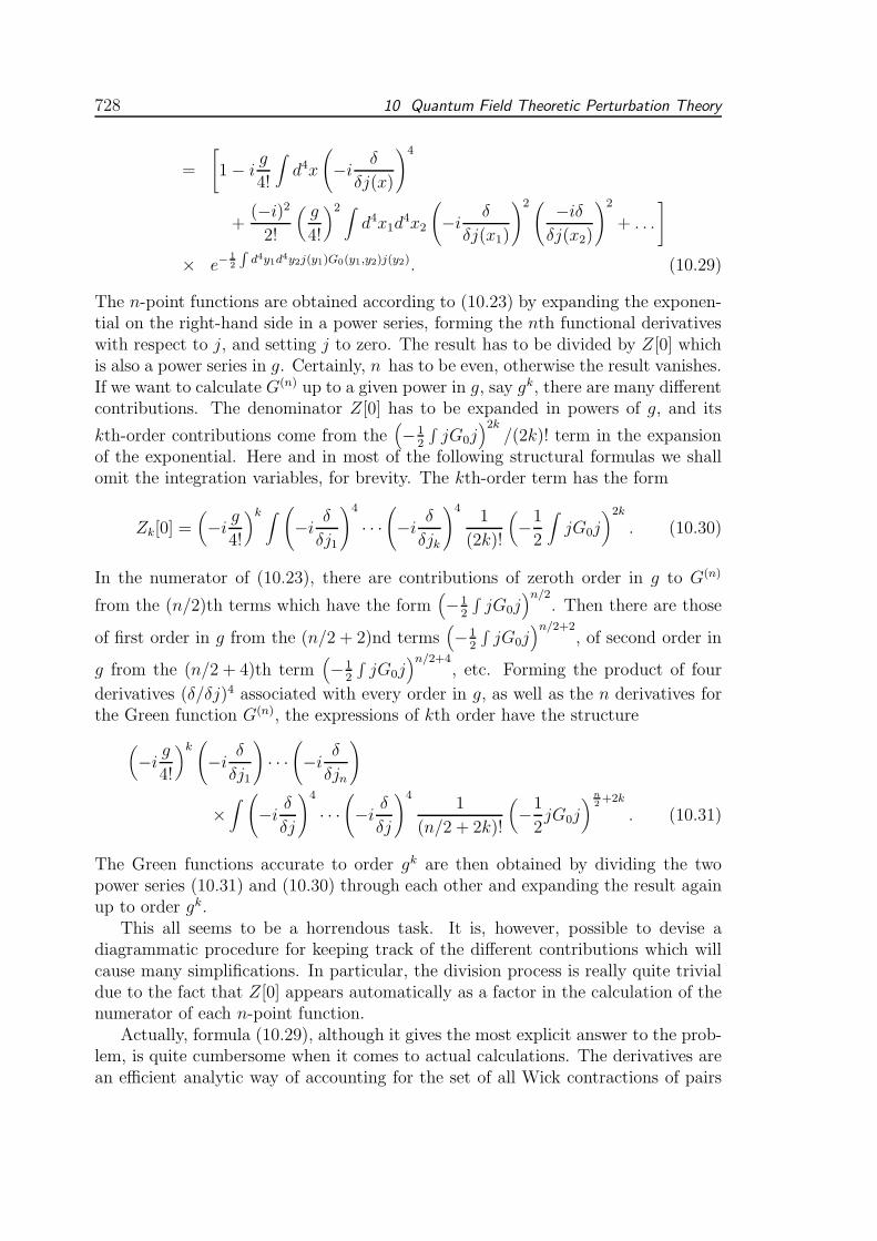
The n-point functions are obtained according to (10.23) by expanding the exponen-tial on the right-hand side in a power series, forming the nth functional derivativeswith respect to j, and setting j to zero. The result has to be divided by Z[0] whichis also a power series in g. Certainly, n has to be even, otherwise the result vanishes.If we want to calculate G(n) up to a given power in g, say gk, there are many differentcontributions. The denominator Z[0] has to be expanded in powers of g, and its
kth-order contributions come from the(
−12
∫
jG0j)2k
/(2k)! term in the expansionof the exponential. Here and in most of the following structural formulas we shallomit the integration variables, for brevity. The kth-order term has the form
Zk[0] =(
−i g4!
)k ∫(
−i δδj1
)4
· · ·(
−i δδjk
)41
(2k)!
(
−1
2
∫
jG0j)2k
. (10.30)
In the numerator of (10.23), there are contributions of zeroth order in g to G(n)
from the (n/2)th terms which have the form(
−12
∫
jG0j)n/2
. Then there are those
of first order in g from the (n/2 + 2)nd terms(
−12
∫
jG0j)n/2+2
, of second order in
g from the (n/2 + 4)th term(
−12
∫
jG0j)n/2+4
, etc. Forming the product of four
derivatives (δ/δj)4 associated with every order in g, as well as the n derivatives forthe Green function G(n), the expressions of kth order have the structure
(
−i g4!
)k(
−i δδj1
)
· · ·(
−i δδjn
)
×∫
(
−i δδj
)4
· · ·(
−i δδj
)41
(n/2 + 2k)!
(
−1
2jG0j
)
n2+2k
. (10.31)
The Green functions accurate to order gk are then obtained by dividing the twopower series (10.31) and (10.30) through each other and expanding the result againup to order gk.
This all seems to be a horrendous task. It is, however, possible to devise adiagrammatic procedure for keeping track of the different contributions which willcause many simplifications. In particular, the division process is really quite trivialdue to the fact that Z[0] appears automatically as a factor in the calculation of thenumerator of each n-point function.
Actually, formula (10.29), although it gives the most explicit answer to the prob-lem, is quite cumbersome when it comes to actual calculations. The derivatives arean efficient analytic way of accounting for the set of all Wick contractions of pairs
10.3 Feynman Rules for φ4-Theory 729
of field operations. In the calculation of a specific n-point function, however, it ismuch more advantageous to insert the expansion (10.18) into formula (10.16), andto separate numerator and denominator by writing
G(n) (x1, . . . , xn) ≡1
Z[0]G(n) (x1, . . . , xn) . (10.32)
Here the unnormalized Green function G(n) (x1, . . . , xn) is the unnormalized Greenfunction. This has the expansion
G(n) (x1, . . . , xn) ≡
= 〈0|T(
1− ig
4!
∫
d4zφ(z) +1
2!
(−ig4!
)2 ∫
d4z1d4z2φ
4(z1)φ4(z2) + . . .
)
× φ(x1) · · ·φ(xn)
|0〉, (10.33)
whereas the denominator Z[0] in (10.32) has the series
Z[0]=〈0|T(
1− ig
4!
∫
d4zφ4(z) +1
2!
(−ig4!
)2 ∫
d4z1d4z2φ
4(z1)φ4(z2)+ . . .
)
|0〉.(10.34)
By performing the Wick contractions in the two expansions explicitly we obtain G(n)p
and Zp[0], respectively, to be divided by one another.
10.3.1 The Vacuum Graphs
Because of its formal simplicity let us start a more explicit perturbation expansionwith the calculation of Z[0]. To first-order in the coupling constant g we have toevaluate
Z1[0] = −i g4!
∫
d4z〈0|T (φ(z)φ(z)φ(z)φ(z)) |0〉, (10.35)
where we have written down the four powers of φ(z) separately in order to seebetter how to perform all pair contractions. The first field can be contracted withthe three others. After this the second field has only one choice. Thus there are 3 ·1contractions, all of the form
−i g4!
∫
d4zG0(z, z)G0(z, z), (10.36)
so that
Z1[0] = −i3 g4!
∫
d4zG0(z, z)G0(z, z). (10.37)
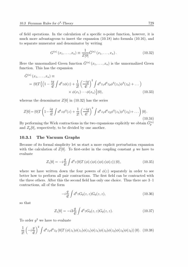
To order g2 we have to evaluate
1
2!
(
−i g4!
)2 ∫
d4z1d4z2 〈0|T (φ(z1)φ(z1)φ(z1)φ(z1)φ(z2)φ(z2)φ(z2)φ(z2)) |0〉. (10.38)
730 10 Quantum Field Theoretic Perturbation Theory
Expanding the expectation value of the product of eight fields into a sum over paircontractions, we obtain 7 · 5 · 3 · 1 = 105 contractions, 32 of them with φ(z1)’s andφ(z2)’s contracting among each other, for example,
φ(z1)φ(z1)φ(z1)φ(z1)|φ(z2)φ(z2)φ(z2)φ(z2), (10.39)
where we have explicitly separated the two interactions by a vertical line. Thereare further 4 · 3 · 2 = 24 contractions, where each φ(z1) connects with a φ(z2), forexample,
φ(z1)φ(z1)φ(z1)φ(z1)|φ(z2)φ(z2)φ(z2)φ(z2), (10.40)
and 6 · 6 · 2 = 72 of the mixed type, for example,
φ(z1)φ(z1)φ(z1)φ(z1)|φ(z2)φ(z2)φ(z2)φ(z2) . (10.41)
The factors six counts the six choices of one contraction within each factor φ4 afterwhich there are only two possible interconnections.The 105 terms obtained in this way correspond to the following integrals
1
2!
(
−i g4!
)2[
9(∫
d4z1G0(z1, z1)2)2
+ 24∫
d4z1d4z1G0 (z1, z2)
4
+ 72∫
d4zd4zG0(z1, z1)G0(z1, z2)2G0 (z1, z2)
2G0(z2, z2)]
. (10.42)
It is useful to picture the different contributions by means of so-called Feynman
diagrams: A line with x1, x2 at the ends
q qx1 x2
= G0(x1, x2) (10.43)
represents a free-particle propagator. A vertex with four emerging lines
z= −i g
4!(10.44)
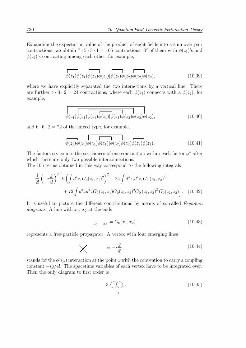
stands for the φ4(z) interaction at the point z with the convention to carry a couplingconstant −ig/4!. The spacetime variables of each vertex have to be integrated over.Then the only diagram to first order is
3 q♥♥. (10.45)
z1
10.3 Feynman Rules for φ4-Theory 731
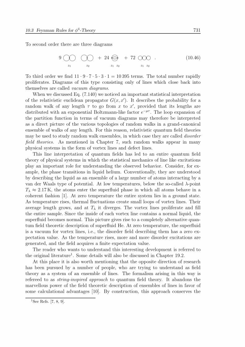
To second order there are three diagrams
9 q♥♥ q♥♥ + 24 q q♥................................................................................ + 72 q q . (10.46)
z1 z2 z1 z2 z1 z2
To third order we find 11 · 9 · 7 · 5 · 3 · 1 = 10 395 terms. The total number rapidlyproliferates. Diagrams of this type consisting only of lines which close back intothemselves are called vacuum diagrams.
When we discussed Eq. (7.140) we noticed an important statistical interpretationof the relativistic euclidean propagator G(x, x′). It describes the probability for arandom walk of any length τ to go from x to x′, provided that its lengths aredistributed with an exponential Boltzmann-like factor e−µτ . The loop expansion ofthe partition function in terms of vacuum diagrams may therefore be interpretedas a direct picture of the various topologies of random walks in a grand-canonicalensemble of walks of any length. For this reason, relativistic quantum field theoriesmay be used to study random walk ensembles, in which case they are called disorder
field theories. As mentioned in Chapter 7, such random walks appear in manyphysical systems in the form of vortex lines and defect lines.
This line interpretation of quantum fields has led to an entire quantum fieldtheory of physical systems in which the statistical mechanics of line like excitationsplay an important role for understanding the observed behavior. Consider, for ex-ample, the phase transitions in liquid helium. Conventionally, they are understoodby describing the liquid as an ensemble of a large number of atoms interacting by avan der Waals type of potential. At low temperatures, below the so-called λ-pointTλ ≈ 2.17K, the atoms enter the superfluid phase in which all atoms behave in acoherent fashion [1]. At zero temperature the entire system lies in a ground state.As temperature rises, thermal fluctuations create small loops of vortex lines. Theiraverage length grows, and at Tλ it diverges. The vortex lines proliferate and fillthe entire sample. Since the inside of each vortex line contains a normal liquid, thesuperfluid becomes normal. This picture gives rise to a completely alternative quan-tum field theoretic description of superfluid He. At zero temperature, the superfluidis a vacuum for vortex lines, i.e., the disorder field describing them has a zero ex-pectation value. As the temperature rises, more and more disorder excitations aregenerated, and the field acquires a finite expectation value.
The reader who wants to understand this interesting development is referred tothe original literature1. Some details will also be discussed in Chapter 19.2.
At this place it is also worth mentioning that the opposite direction of researchhas been pursued by a number of people, who are trying to understand as fieldtheory as a system of an ensemble of lines. The formalism arising in this way isrefereed to as string-inspired approach to quantum field theory. It abandons themarvellous power of the field theoretic description of ensembles of lines in favor ofsome calculational advantages [10]. By construction, this approach conserves the
1See Refs. [7, 8, 9].
732 10 Quantum Field Theoretic Perturbation Theory
number of lines, i.e., the number of particles. Thus it will not be efficient whenparticle condensation processes are important, since then vortex line numbers arecertainly not conserved.
10.4 The Two-Point Function
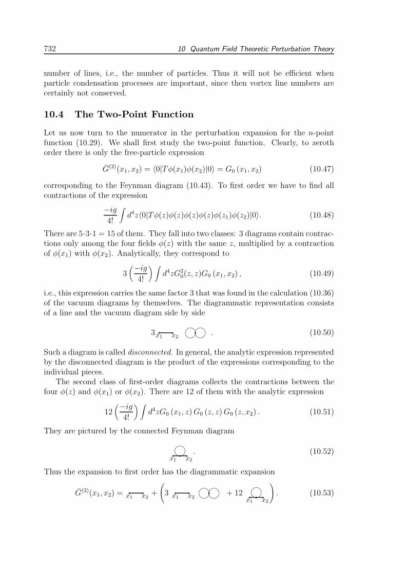
Let us now turn to the numerator in the perturbation expansion for the n-pointfunction (10.29). We shall first study the two-point function. Clearly, to zerothorder there is only the free-particle expression
G(2)(x1, x2) = 〈0|Tφ(x1)φ(x2)|0〉 = G0 (x1, x2) (10.47)
corresponding to the Feynman diagram (10.43). To first order we have to find allcontractions of the expression
−ig4!
∫
d4z〈0|Tφ(z)φ(z)φ(z)φ(z)φ(z1)φ(z2)|0〉. (10.48)
There are 5·3·1 = 15 of them. They fall into two classes: 3 diagrams contain contrac-tions only among the four fields φ(z) with the same z, multiplied by a contractionof φ(x1) with φ(x2). Analytically, they correspond to
3(−ig
4!
) ∫
d4zG20(z, z)G0 (x1, x2) , (10.49)
i.e., this expression carries the same factor 3 that was found in the calculation (10.36)of the vacuum diagrams by themselves. The diagrammatic representation consistsof a line and the vacuum diagram side by side
3 q qx1 x2
q♥♥. (10.50)
Such a diagram is called disconnected. In general, the analytic expression representedby the disconnected diagram is the product of the expressions corresponding to theindividual pieces.
The second class of first-order diagrams collects the contractions between thefour φ(z) and φ(x1) or φ(x2). There are 12 of them with the analytic expression
12(−ig
4!
)∫
d4zG0 (x1, z)G0 (z, z)G0 (z, x2) . (10.51)
They are pictured by the connected Feynman diagram
♥q qx1 x2
q . (10.52)
Thus the expansion to first order has the diagrammatic expansion
G(2)(x1, x2) = q qx1 x2
+
(
3 q qx1 x2
q♥♥ + 12 ♥q qx1 x2
q
)
. (10.53)
10.4 The Two-Point Function 733
Remembering the expansion of the denominator to this order
Z[0] = 1 + 3 q♥♥ , (10.54)
we see that the two-particle Green function is, to order g, given by the free diagramplus the diagram in Fig. 10.52:
G(2)(x1, x2) = q qx1 x2
+ 12 ♥q qx1 x2
q . (10.55)
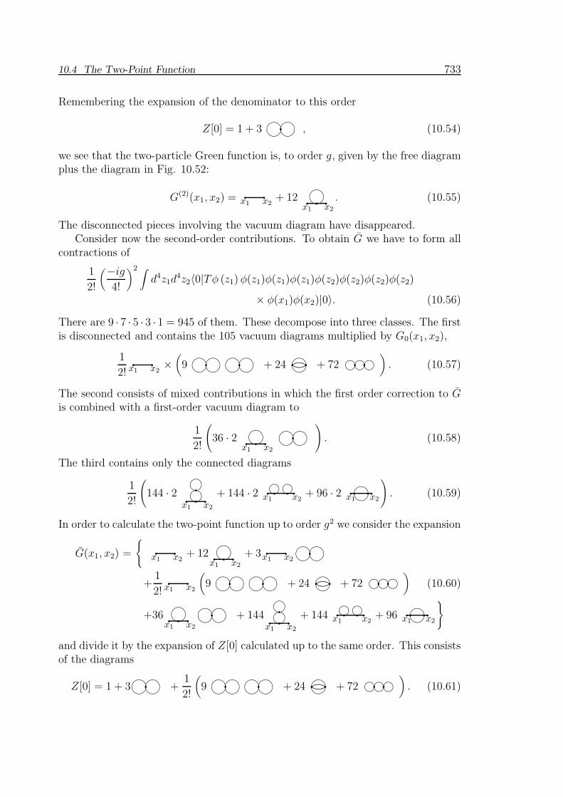
The disconnected pieces involving the vacuum diagram have disappeared.Consider now the second-order contributions. To obtain G we have to form all
contractions of
1
2!
(−ig4!
)2 ∫
d4z1d4z2〈0|Tφ (z1)φ(z1)φ(z1)φ(z1)φ(z2)φ(z2)φ(z2)φ(z2)
× φ(x1)φ(x2)|0〉. (10.56)
There are 9 · 7 · 5 · 3 · 1 = 945 of them. These decompose into three classes. The firstis disconnected and contains the 105 vacuum diagrams multiplied by G0(x1, x2),
1
2!q q
x1 x2×(
9 q♥♥ q♥♥ + 24 q q♥................................................................................ + 72 q q
)
. (10.57)
The second consists of mixed contributions in which the first order correction to Gis combined with a first-order vacuum diagram to
1
2!
(
36 · 2 ♥q qx1 x2
q q♥♥)
. (10.58)
The third contains only the connected diagrams
1
2!
(
144 · 2 qqq q
x1 x2
+ 144 · 2 q q
x1 x2
q q + 96 · 2 ♥q qq qx1 x2
)
. (10.59)
In order to calculate the two-point function up to order g2 we consider the expansion
G(x1, x2) =
q qx1 x2
+ 12 ♥q qx1 x2
q + 3 q qx1 x2
q♥♥
+1
2!q q
x1 x2
(
9 q♥♥ q♥♥ + 24 q q♥................................................................................ + 72 q q
)
(10.60)
+36 ♥q qx1 x2
q q♥♥ + 144qqq q
x1 x2
+ 144 q q
x1 x2
q q + 96 ♥q qq qx1 x2
and divide it by the expansion of Z[0] calculated up to the same order. This consistsof the diagrams
Z[0] = 1 + 3 q♥♥ +1
2!
(
9 q♥♥ q♥♥ + 24 q q♥................................................................................ + 72 q q
)
. (10.61)
734 10 Quantum Field Theoretic Perturbation Theory
Dividing G(x1, x2) by Z[0] gives the two-point function
G(2)(x1, x2) = q qx1 x2
+ 12 ♥q qx1 x2
q
+1
2!
(
144 · 2 qqq q
x1 x2
+ 144 · 2 q q
x1 x2
q q + 96 · 2 ♥q qq qx1 x2
)
+ . . . . (10.62)
10.5 The Four-Point Function
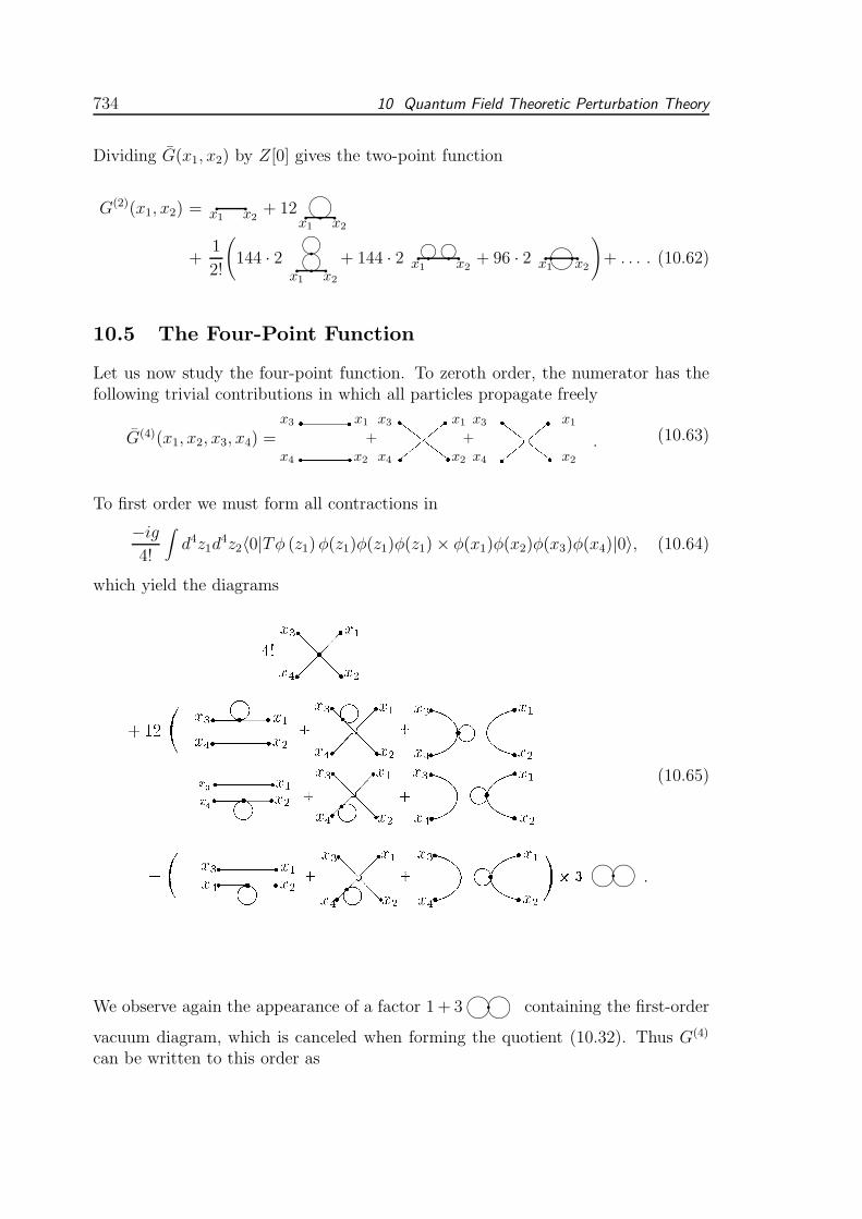
Let us now study the four-point function. To zeroth order, the numerator has thefollowing trivial contributions in which all particles propagate freely
G(4)(x1, x2, x3, x4) =x1
x2
x3
x4
x1
x2
x3
x4
x3
x4
x1
x2
+ + . (10.63)
To first order we must form all contractions in
−ig4!
∫
d4z1d4z2〈0|Tφ (z1)φ(z1)φ(z1)φ(z1)× φ(x1)φ(x2)φ(x3)φ(x4)|0〉, (10.64)
which yield the diagrams
q♥♥.
(10.65)
We observe again the appearance of a factor 1 + 3 q♥♥ containing the first-order
vacuum diagram, which is canceled when forming the quotient (10.32). Thus G(4)
can be written to this order as
10.5 The Four-Point Function 735
G(4)(x1, . . . , xn) =
. (10.66)
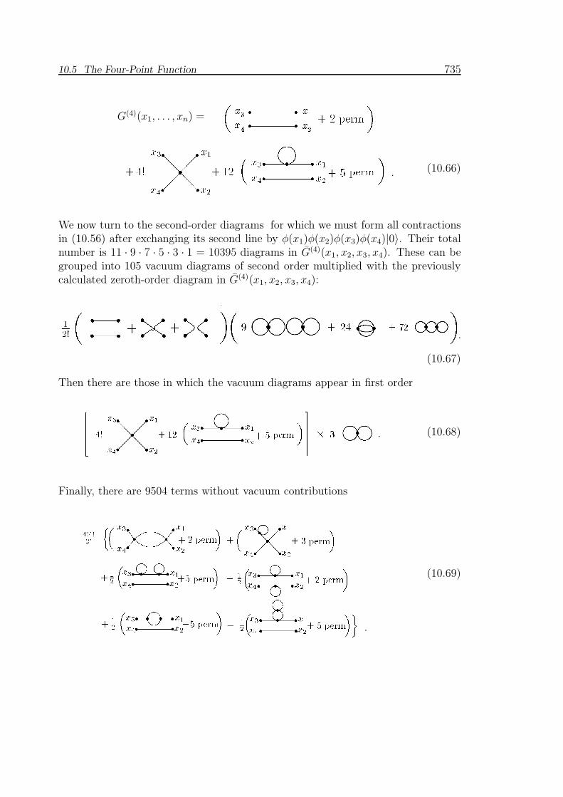
We now turn to the second-order diagrams for which we must form all contractionsin (10.56) after exchanging its second line by φ(x1)φ(x2)φ(x3)φ(x4)|0〉. Their totalnumber is 11 · 9 · 7 · 5 · 3 · 1 = 10395 diagrams in G(4)(x1, x2, x3, x4). These can begrouped into 105 vacuum diagrams of second order multiplied with the previouslycalculated zeroth-order diagram in G(4)(x1, x2, x3, x4):
.
(10.67)
Then there are those in which the vacuum diagrams appear in first order
. (10.68)
Finally, there are 9504 terms without vacuum contributions
.
(10.69)
736 10 Quantum Field Theoretic Perturbation Theory
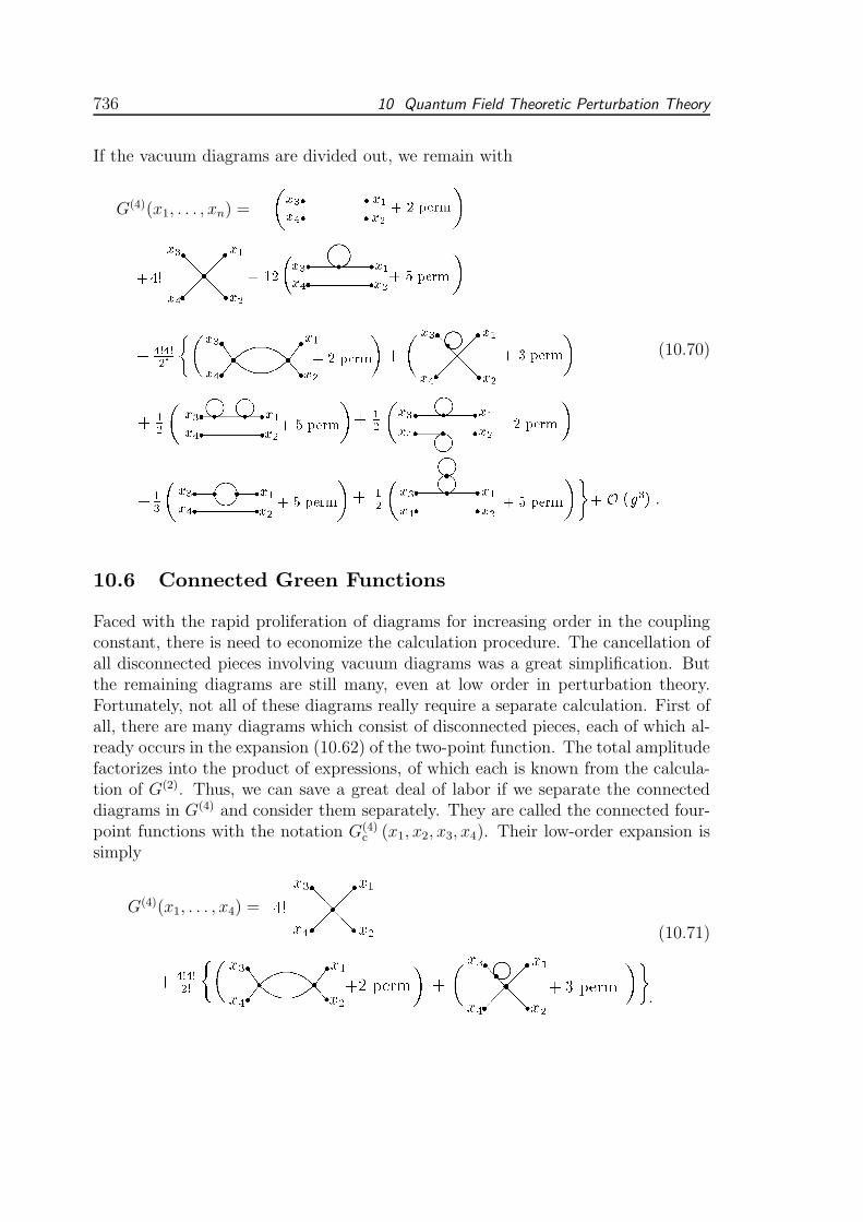
If the vacuum diagrams are divided out, we remain with
G(4)(x1, . . . , xn) =
.
(10.70)
10.6 Connected Green Functions
Faced with the rapid proliferation of diagrams for increasing order in the couplingconstant, there is need to economize the calculation procedure. The cancellation ofall disconnected pieces involving vacuum diagrams was a great simplification. Butthe remaining diagrams are still many, even at low order in perturbation theory.Fortunately, not all of these diagrams really require a separate calculation. First ofall, there are many diagrams which consist of disconnected pieces, each of which al-ready occurs in the expansion (10.62) of the two-point function. The total amplitudefactorizes into the product of expressions, of which each is known from the calcula-tion of G(2). Thus, we can save a great deal of labor if we separate the connecteddiagrams in G(4) and consider them separately. They are called the connected four-point functions with the notation G(4)
c (x1, x2, x3, x4). Their low-order expansion issimply
G(4)(x1, . . . , x4) =
.
(10.71)
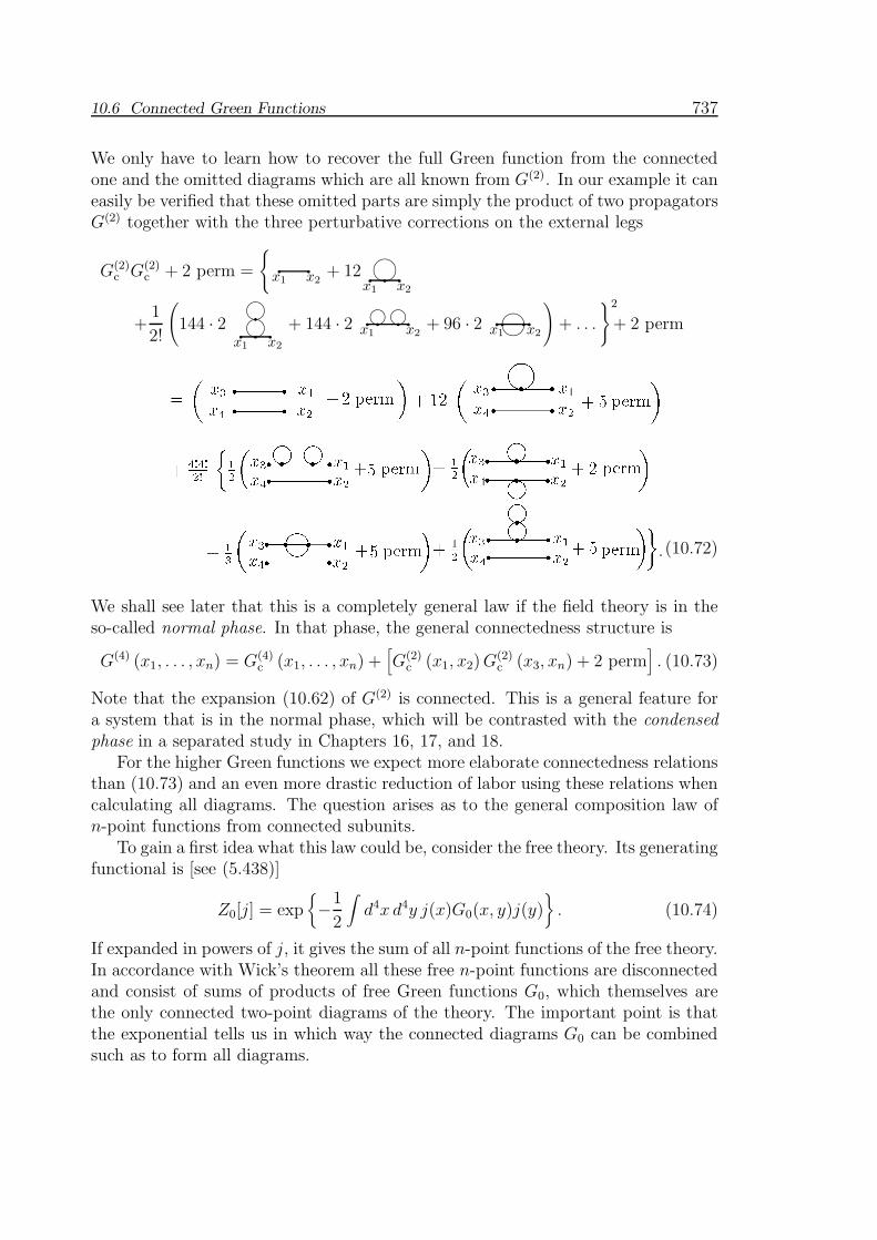
10.6 Connected Green Functions 737
We only have to learn how to recover the full Green function from the connectedone and the omitted diagrams which are all known from G(2). In our example it caneasily be verified that these omitted parts are simply the product of two propagatorsG(2) together with the three perturbative corrections on the external legs
G(2)c G(2)
c + 2 perm =
q qx1 x2
+ 12 ♥q qx1 x2
q
+1
2!
(
144 · 2 qqq q
x1 x2
+ 144 · 2 q q
x1 x2
q q + 96 · 2 ♥q qq qx1 x2
)
+ . . .
2
+ 2 perm
.(10.72)
We shall see later that this is a completely general law if the field theory is in theso-called normal phase. In that phase, the general connectedness structure is
G(4) (x1, . . . , xn) = G(4)c (x1, . . . , xn) +
[
G(2)c (x1, x2)G
(2)c (x3, xn) + 2 perm
]
. (10.73)
Note that the expansion (10.62) of G(2) is connected. This is a general feature fora system that is in the normal phase, which will be contrasted with the condensed
phase in a separated study in Chapters 16, 17, and 18.For the higher Green functions we expect more elaborate connectedness relations
than (10.73) and an even more drastic reduction of labor using these relations whencalculating all diagrams. The question arises as to the general composition law ofn-point functions from connected subunits.
To gain a first idea what this law could be, consider the free theory. Its generatingfunctional is [see (5.438)]
Z0[j] = exp
−1
2
∫
d4x d4y j(x)G0(x, y)j(y)
. (10.74)
If expanded in powers of j, it gives the sum of all n-point functions of the free theory.In accordance with Wick’s theorem all these free n-point functions are disconnectedand consist of sums of products of free Green functions G0, which themselves arethe only connected two-point diagrams of the theory. The important point is thatthe exponential tells us in which way the connected diagrams G0 can be combinedsuch as to form all diagrams.
738 10 Quantum Field Theoretic Perturbation Theory
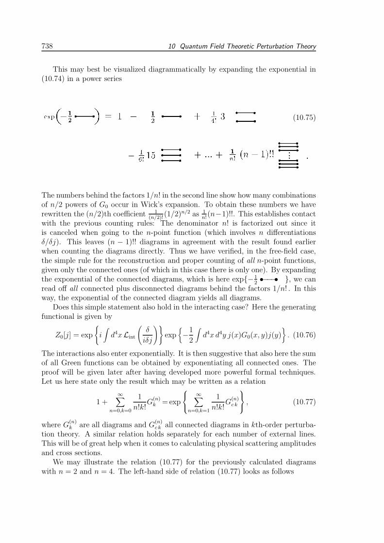
This may best be visualized diagrammatically by expanding the exponential in(10.74) in a power series
(10.75)
The numbers behind the factors 1/n! in the second line show how many combinationsof n/2 powers of G0 occur in Wick’s expansion. To obtain these numbers we haverewritten the (n/2)th coefficient 1
(n/2)!(1/2)n/2 as 1
n!(n−1)!!. This establishes contact
with the previous counting rules: The denominator n! is factorized out since itis canceled when going to the n-point function (which involves n differentiationsδ/δj). This leaves (n − 1)!! diagrams in agreement with the result found earlierwhen counting the diagrams directly. Thus we have verified, in the free-field case,the simple rule for the reconstruction and proper counting of all n-point functions,given only the connected ones (of which in this case there is only one). By expandingthe exponential of the connected diagrams, which is here exp−1
2•−−−• , we can
read off all connected plus disconnected diagrams behind the factors 1/n! . In thisway, the exponential of the connected diagram yields all diagrams.
Does this simple statement also hold in the interacting case? Here the generatingfunctional is given by
Z0[j] = exp
i∫
d4xLint
(
δ
iδj
)
exp
−1
2
∫
d4x d4y j(x)G0(x, y)j(y)
. (10.76)
The interactions also enter exponentially. It is then suggestive that also here the sumof all Green functions can be obtained by exponentiating all connected ones. Theproof will be given later after having developed more powerful formal techniques.Let us here state only the result which may be written as a relation
1 +∞∑
n=0,k=0
1
n!k!G
(n)k =exp
∞∑
n=0,k=1
1
n!k!G
(n)c k
, (10.77)
where G(n)k are all diagrams and G
(n)c k all connected diagrams in kth-order perturba-
tion theory. A similar relation holds separately for each number of external lines.This will be of great help when it comes to calculating physical scattering amplitudesand cross sections.
We may illustrate the relation (10.77) for the previously calculated diagramswith n = 2 and n = 4. The left-hand side of relation (10.77) looks as follows

10.6 Connected Green Functions 739
(10.78)
The right-hand side has the form
(10.79)
Indeed, by multiplying out the square in the last line we recover the correct sum ofdisconnected diagrams of the four-point function.
Also the vacuum diagrams satisfy the law of exponentiation: Up to the secondorder we have for all disconnected pieces
Z[0] = 1+3 q♥♥+1
2!
(
9 q♥♥ q♥♥ + 24 q q♥................................................................................ + 72 q q
)
+. . . , (10.80)
and see that this can be obtained as an exponential of the connected vacuum dia-grams
Z[0] = exp
3 q♥♥ +1
2!
(
24 q q♥................................................................................ + 72 q q
)
+ . . .
≡ eW [0]. (10.81)
740 10 Quantum Field Theoretic Perturbation Theory
This corresponds to equation (10.77) for n = 0:
1 +∞∑
k=0
1
k!G
(0)k = exp
[
∞∑
k=1
1
k!G
(0)c k
]
, (10.82)
where G(0)k collect all vacuum diagrams and G
(0)c k all connected ones in kth-order
perturbation theory.
10.6.1 One-Particle Irreducible Graphs
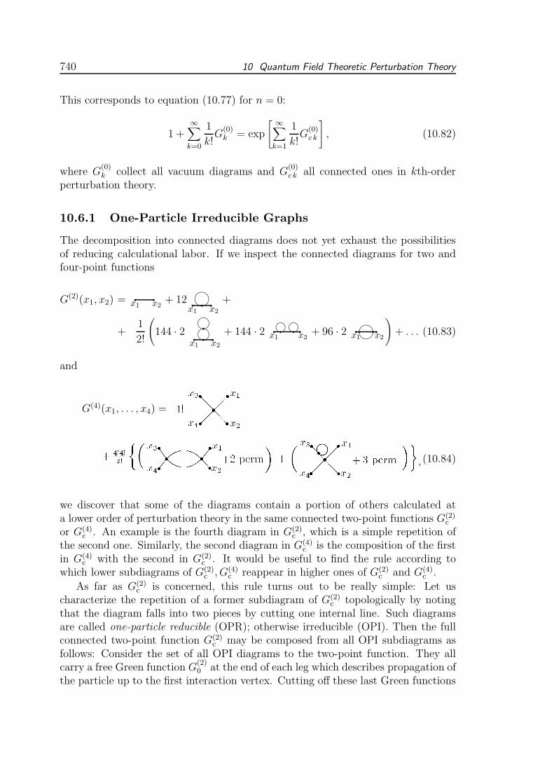
The decomposition into connected diagrams does not yet exhaust the possibilitiesof reducing calculational labor. If we inspect the connected diagrams for two andfour-point functions
G(2)(x1, x2) = q qx1 x2
+ 12 ♥q qx1 x2
q +
+1
2!
(
144 · 2 qqq q
x1 x2
+ 144 · 2 q q
x1 x2
q q + 96 · 2 ♥q qq qx1 x2
)
+ . . . (10.83)
and
G(4)(x1, . . . , x4) =
, (10.84)
we discover that some of the diagrams contain a portion of others calculated ata lower order of perturbation theory in the same connected two-point functions G(2)
c
or G(4)c . An example is the fourth diagram in G(2)
c , which is a simple repetition ofthe second one. Similarly, the second diagram in G(4)
c is the composition of the firstin G(4)
c with the second in G(2)c . It would be useful to find the rule according to
which lower subdiagrams of G(2)c , G(4)
c reappear in higher ones of G(2)c and G(4)
c .
As far as G(2)c is concerned, this rule turns out to be really simple: Let us
characterize the repetition of a former subdiagram of G(2)c topologically by noting
that the diagram falls into two pieces by cutting one internal line. Such diagramsare called one-particle reducible (OPR); otherwise irreducible (OPI). Then the fullconnected two-point function G(2)
c may be composed from all OPI subdiagrams asfollows: Consider the set of all OPI diagrams to the two-point function. They allcarry a free Green function G
(2)0 at the end of each leg which describes propagation of
the particle up to the first interaction vertex. Cutting off these last Green functions

10.6 Connected Green Functions 741
amounts diagramically to amputating the two legs of the diagram. The lowest ordercorrection to the two-point function is amputated as follows:
.
The two short little trunks indicate the places of amputation. Let −iΣ be the sumof all these amputated OPI two-point functions. Then the geometric series
G(2)c =
1
G−10 + Σ
= G0 +G0(−iΣ)G0 +G0(−iΣ)G0 + . . . (10.85)
gives precisely the connected two-point function G(2)c . Thus the one-particle re-
ducibility in the two-point function exhausts itself in a simple geometric series typeof repetition of the irreducible pieces, each term in the string having the same factor.Also this result will be proved later in Chapter 13 when studying the general formalproperties of perturbation theory.
The sum of all OPI connected two-point functions −iΣ is usually referred to asself-energy.
Consider now the four-point function G(4)c . Here we recognize that any ornamen-
tation of external legs can be taken care of by replacing the legs by the interactingtwo-point function. Thus we decide to introduce the concept of an arbitrary one-particle irreducible amputated Green function, shortly called the vertex function
Γ(n) (x1, . . . , xn). For any connected n-point function, cut all simple lines such thatthe diagrams decompose. What remains are parts with two, four, or more trunkssticking out. The first set consists of the OPI self-energy diagrams discussed before.The others are called three-, four-, n-point vertex parts Γ(n), n = 3, 4, . . . . Forexample,
can be cut into four proper self-energy diagrams and one four-point vertex part.The sum of all composite diagrams obtained in this way composes the n-point ver-tex function denoted by a fat dot. The important reconstruction principle for alldiagrams can now be states as follows: The set of all connected diagrams in a four-point function is obtained by connecting all vertex functions in the four-point vertexfunction G(4)
c with the full connected Green function G(2)c at each truncated leg. An-
alytically, this amounts to the formula (valid in normal systems)
742 10 Quantum Field Theoretic Perturbation Theory
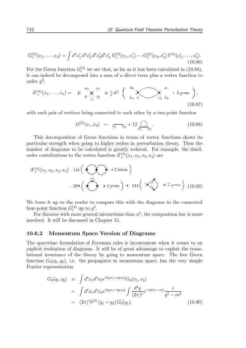
G(4)c (x1, . . . , x4) =
∫
d4x′1 d4x′2 d
4x′3d4x′4 G
(2)c (x1, x
′1) · · ·G(2)
c (x4, x′4) Γ
(4)(x′1, . . . , x′4).
(10.86)
For the Green function G(4)c we see that, as far as it has been calculated in (10.84),
it can indeed be decomposed into a sum of a direct term plus a vertex function toorder g2:
iΓ(4)c (x1, . . . , xn) = ,
(10.87)
with each pair of vertices being connected to each other by a two-point function
G(2)(x1, x2) = q qx1 x2
+ 12 ♥q qx1 x2
q . (10.88)
This decomposition of Green functions in terms of vertex functions shows itsparticular strength when going to higher orders in perturbation theory. Then thenumber of diagrams to be calculated is greatly reduced. For example, the third-order contributions to the vertex function iΓ(4)
c (x1, x2, x3, x4) are
iΓ(4)c (x1, x2, x3, x4)
.(10.89)
We leave it up to the reader to compare this with the diagrams in the connectedfour-point function G(4)
c up to g3.For theories with more general interactions than φ4, the composition law is more
involved. It will be discussed in Chapter 15.
10.6.2 Momentum Space Version of Diagrams
The spacetime formulation of Feynman rules is inconvenient when it comes to anexplicit evaluation of diagrams. It will be of great advantage to exploit the trans-lational invariance of the theory by going to momentum space. The free Greenfunction G0(q1, q2), i.e. the propagator in momentum space, has the very simpleFourier representation
G0(q1, q2) ≡∫
d4x1d4x2e
i(q1x1+q2x2)G0(x1, x2)
=∫
d4x1d4x2e
i(q1x1+q2x2)∫
d4q
(2π)4e−iq(x1−x2)
i
q2 −m2
= (2π)4δ(4) (q1 + q2)G0(q1). (10.90)
10.6 Connected Green Functions 743
There is an overall (2π)4 δ(4)-function which ensures the conservation of four-momenta. This is a consequence of the translational invariance of G0 (x1, x2) =G0 (x1 − x2). The same factor appears in the Fourier transform of all interactingn-point functions since G(n) (x1, . . . , x1) depends only on the differences between thecoordinates
G(n)(x1, . . . , xn) = G(n)(x1 − xn, x2 − xn, . . . , xn−1 − xn, 0) (10.91)
such that we can write∫
d4x1 . . . d4xne
iΣni=1
qixiG(n)(x1, . . . xn)
=∫
d4(x1 − xn) · · · d4(xn−1 − xn)ei∑n−1
i=1qi(xi−xn)
(∫
d4xneiΣ∞
i=1qixn
)
×G(n)(x1 − xn, x2 − xn, . . . , xn−1 − xn, 0) . (10.92)
Thus we may define the Fourier transform of an n-point function directly withoutthe factor of momentum conservation as
(2π)4δ(4) (q1 + . . .+ qn)G(n) (q1, . . . , qn)≡
∫
d4x1 · · · d4xn eiΣni=1
qixiG(n) (x1, . . . , xn) .
(10.93)
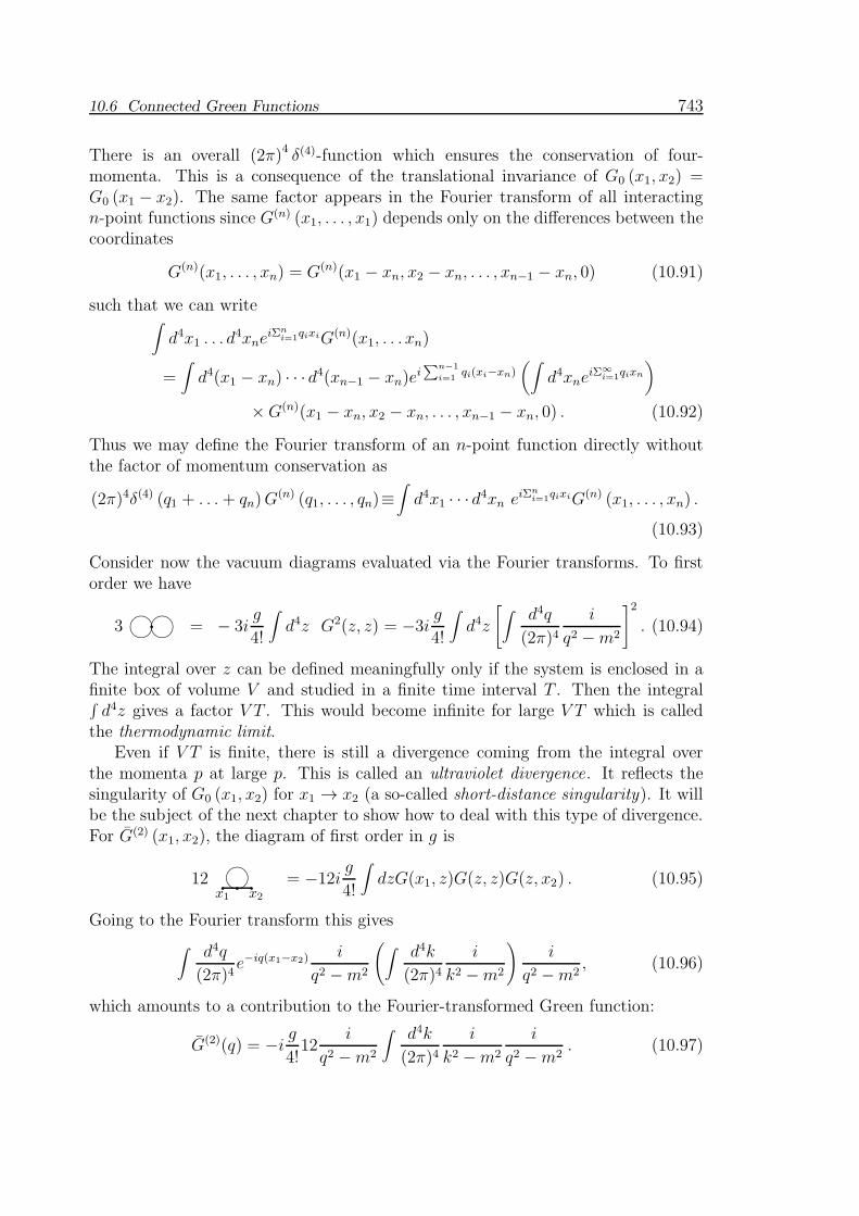
Consider now the vacuum diagrams evaluated via the Fourier transforms. To firstorder we have
3 q♥♥ = − 3ig
4!
∫
d4z G2(z, z) = −3ig
4!
∫
d4z
[
∫ d4q
(2π)4i
q2 −m2
]2
. (10.94)
The integral over z can be defined meaningfully only if the system is enclosed in afinite box of volume V and studied in a finite time interval T . Then the integral∫
d4z gives a factor V T . This would become infinite for large V T which is calledthe thermodynamic limit.
Even if V T is finite, there is still a divergence coming from the integral overthe momenta p at large p. This is called an ultraviolet divergence. It reflects thesingularity of G0 (x1, x2) for x1 → x2 (a so-called short-distance singularity). It willbe the subject of the next chapter to show how to deal with this type of divergence.For G(2) (x1, x2), the diagram of first order in g is
12 ♥q qx1 x2
q = −12ig
4!
∫
dzG(x1, z)G(z, z)G(z, x2) . (10.95)
Going to the Fourier transform this gives
∫
d4q
(2π)4e−iq(x1−x2)
i
q2 −m2
(
∫
d4k
(2π)4i
k2 −m2
)
i
q2 −m2, (10.96)
which amounts to a contribution to the Fourier-transformed Green function:
G(2)(q) = −i g4!12
i
q2 −m2
∫
d4k
(2π)4i
k2 −m2
i
q2 −m2. (10.97)
744 10 Quantum Field Theoretic Perturbation Theory
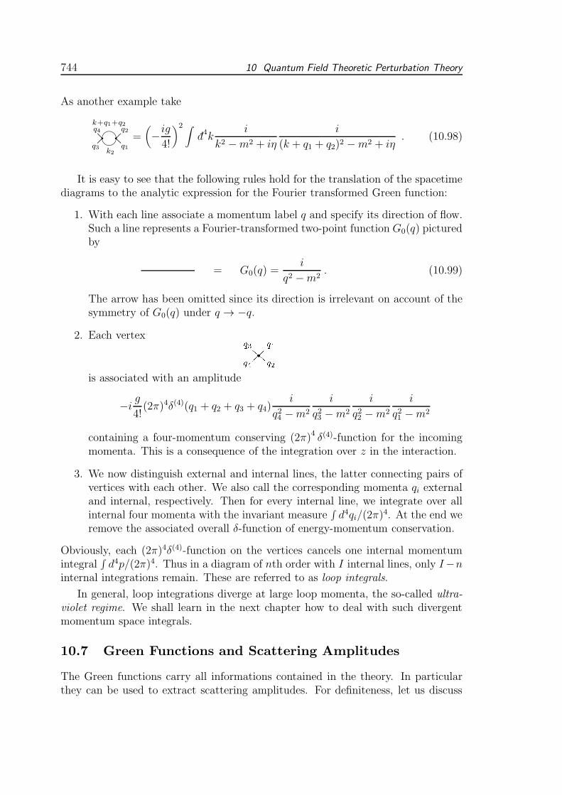
As another example take
♥q q ....................................
....................................
q3
q4
q1
q2
k2
k+q1+q2
=(
−ig4!
)2 ∫
-d4ki
k2 −m2 + iη
i
(k + q1 + q2)2 −m2 + iη. (10.98)
It is easy to see that the following rules hold for the translation of the spacetimediagrams to the analytic expression for the Fourier transformed Green function:
1. With each line associate a momentum label q and specify its direction of flow.Such a line represents a Fourier-transformed two-point function G0(q) picturedby
= G0(q) =i
q2 −m2. (10.99)
The arrow has been omitted since its direction is irrelevant on account of thesymmetry of G0(q) under q → −q.
2. Each vertex
is associated with an amplitude
−i g4!(2π)4δ(4)(q1 + q2 + q3 + q4)
i
q24 −m2
i
q23 −m2
i
q22 −m2
i
q21 −m2
containing a four-momentum conserving (2π)4 δ(4)-function for the incomingmomenta. This is a consequence of the integration over z in the interaction.
3. We now distinguish external and internal lines, the latter connecting pairs ofvertices with each other. We also call the corresponding momenta qi externaland internal, respectively. Then for every internal line, we integrate over allinternal four momenta with the invariant measure
∫
d4qi/(2π)4. At the end we
remove the associated overall δ-function of energy-momentum conservation.
Obviously, each (2π)4δ(4)-function on the vertices cancels one internal momentumintegral
∫
d4p/(2π)4. Thus in a diagram of nth order with I internal lines, only I−ninternal integrations remain. These are referred to as loop integrals.
In general, loop integrations diverge at large loop momenta, the so-called ultra-
violet regime. We shall learn in the next chapter how to deal with such divergentmomentum space integrals.
10.7 Green Functions and Scattering Amplitudes
The Green functions carry all informations contained in the theory. In particularthey can be used to extract scattering amplitudes. For definiteness, let us discuss
10.7 Green Functions and Scattering Amplitudes 745
here the simplest and most important case of the elastic scattering among twoparticles. The free initial state that exists long before the interaction takes place is
|ψin〉 = a†q2a†q1
|0〉. (10.100)
Long after the interaction, the state is given by
UηI (∞,−∞) a†q2
a†q1|0〉. (10.101)
If we analyze this state with respect to its free-particle content we find the amplitude
〈0|aq4aq3
UηI (∞,−∞) a†q2
a†q1|0〉 = 〈0|aq4
aq3Sηaq2
aq1|0〉. (10.102)
We shall soon observe that this amplitude has a divergent phase arising in the limitof the switching parameter η tending to zero. It is caused by the same vacuumdiagrams as before in the corresponding Green function. In order to obtain a well-defined η → 0 -limit we define the 2× 2 scattering amplitude as the ratio
S (q4,q3|q1,q2) ≡ SN (q4,q3|q1,q2)
Z[0], (10.103)
with the numerator
SN (q4,q3|q1,q2) ≡ 〈0|aq4aq3
Te−i∫
∞
−∞dt VI(t)a†q2
a†q1|0〉, (10.104)
and the denominator
Z[0] ≡ 〈0|e−i∫
∞
−∞dt VI (t)|0〉. (10.105)
We shall often use the four-momentum notation S (q4, q3|q1, q2) for S (q4,q3|q1,q2)with the tacit understanding that, in the S-matrix, the energies are always on themass shells q0 =
√q2 +m2.
It is now easy to see how these amplitudes can be extracted from the Greenfunctions calculated in the last section. There exists a mathematical framework todo this known as the Lehmann-Symanzik-Zimmermann formalism (LSZ-reductionformulas) [11]. Rather than presenting this we sketch here a simple pedestrianapproach to obtain the same results.
We begin with the observation that if the energies q0 on the mass shells of theparticles, i.e., if q0 = ωq =
√p2 +M2, the particle operators aq, a
†q can be written
as the large-time limits
aq = limx0→−∞
√
2q0
V
∫
d3x ei(q0x0−qx)φ(x), (10.106)
a†q = limx0→∞
√
2q0
V
∫
d3x e−i(q0x0−qx)φ(x). (10.107)

746 10 Quantum Field Theoretic Perturbation Theory
The limits have the important effect of eliminating undesired frequency contents inφ(x). Indeed, if we expand the field into creation and annihilation operators, we seethat the right-hand side of Eq. (10.106) becomes
limx0→−∞
√
2q0V
∫
d3xei(q0x0−qx)
∑
q
1√2p0V
(
e−ipxap + c.c.)
= limx0→−∞
∑
p
δp,q[
ei(q0−p0)x0
ap + ei(q0+p0)x0
a†p]
. (10.108)
The spatial δ-function enforces q = p and thus q0 = p0, so that the right-hand sidebecomes
aq + limx0→−∞
ei2q0x0
a†q. (10.109)
In the limit x0 → −∞, the second exponential function oscillates rapidly withdiverging frequency. Such an oscillating expression can be set equal to zero. Thereason why this makes sense uses the fact that no physical state is completely sharpin momentum space but contains some, possibly very narrow, distribution functionf(q− q′) in the momenta. Thus, instead of aq, we really deal with a packet state
∫
d3q′
(2π)3f(q− q′)aq′ ,
with f(q− q′) sharply peaked around q. Then Eq. (10.114) has to be smeared outwith such a would-be δ-function, and the second term in (10.109) becomes
limx0→−∞
∫
d3q′
(2π)3ei2q
′0x0
f(q− q′)a†q′ → 0 . (10.110)
The vanishing of this in the limit x0 → −∞ is a well-known consequence of theRiemann-Lebesgue Lemma (recall the remarks on p. 262). The other equation(10.107) is proved similarly.
We can now make use of formula (10.107), replace the operators aq, a†q by time-
ordered fields φ(x) and obtain, for the numerator part of the S matrix elements inEq. (10.104), the following expression:
SN (q4q3|q2q1)=
√
24q01q02q
03q
04
V 2lim
x01>x0
2→∞
x04<x0
3→−∞
ei[q0
4x0
4−q4x4+q0
3x0
3−q3x3−q0
2x0
2+q2x2−q0
1x0
1+q1x1]
× 〈0|Tφ(x4)φ(x3)Sφ(x2)φ(x1)|0〉. (10.111)
The last factor is precisely the four-point function G(4) (x4, x3, x2, x1).This formula looks somewhat cumbersome to implement in an actual calcula-
tion of the scattering amplitudes and it is useful to simplify it by evaluating theinfinite-time limits more explicitly. We observe that the perturbation series for
10.7 Green Functions and Scattering Amplitudes 747
G(n) (xn, . . . , x1) consists of sums of products of free two-point functions G0 whichcontain, for each spacetime argument x1, x2, . . . , xn in G(n), a two-point function G0
whose line ends at that point. Consider, for example, the point x1, and an associ-ated Green function G0(z1, x1). The operation (10.108) at this point corresponds totaking the limit
√
2q01V
limx01→−∞
∫
d3x1e−i(q0
1x0
1−q1x1)
∫ d4q
(2π)4e−iq(z−x1)
i
q2 −m2 + iη. (10.112)
The spatial integral over x1 enforces q = q1. The remaining integral over dq0 canbe done via Cauchy’s residue theorem. Since x01 → −∞, the contour of integrationmay be closed in the lower half of the complex q0-plane, where it contains only a
pole at q0 = ωq1=√
q21 +m2 − iη. Thus the integral over q0 can be done trivially,
and we find, that the limit (10.111) has the effect of replacing, in the Green functionG(z, x1) of the external leg, the amplitude by
G(z, x1)−−−→1
√
2q01Ve−iq1z, (10.113)
with q01 on the mass shell q01 =√
q21 +m2. The right-hand side is simply the wave
function e−iq1z/√
2q01V of the incoming particle with the argument z of the nearestvertex in the Feynman diagram.
Similarly, we obtain for an outgoing particle of momentum q3 the replacement
G(x3, z)−−−→1
√
2q03Veiq3z . (10.114)
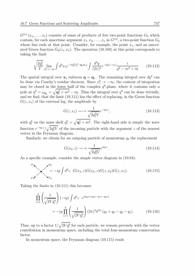
As a specific example, consider the simple vertex diagram in (10.84):
= −ig∫
d4z G(x4, z)G(x3, z)G(z, x2)G(z, x1). (10.115)
Taking the limits in (10.111) this becomes
4∏
i=1
1√
2V q0i
(−ig)∫
d4z ei(q4z+q3z−q1z−q2z)
= −ig4∏
i=1
1√
2V q0i
(2π)4δ(4) (q4 + q3 − q2 − q1) . (10.116)
Thus, up to a factor 1/√
2V q0i for each particle, we remain precisely with the vertexcontribution in momentum space, including the total four-momentum conservationfactor.
In momentum space, the Feynman diagram (10.115) reads
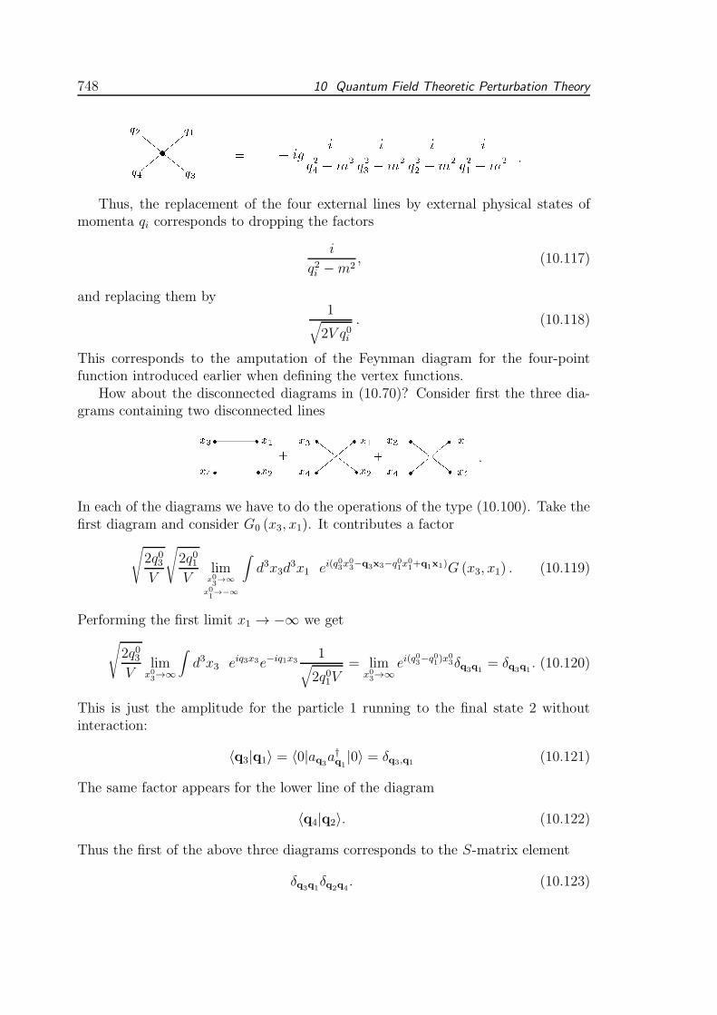
748 10 Quantum Field Theoretic Perturbation Theory
.
Thus, the replacement of the four external lines by external physical states ofmomenta qi corresponds to dropping the factors
i
q2i −m2, (10.117)
and replacing them by1
√
2V q0i. (10.118)
This corresponds to the amputation of the Feynman diagram for the four-pointfunction introduced earlier when defining the vertex functions.
How about the disconnected diagrams in (10.70)? Consider first the three dia-grams containing two disconnected lines
.
In each of the diagrams we have to do the operations of the type (10.100). Take thefirst diagram and consider G0 (x3, x1). It contributes a factor
√
2q03V
√
2q01V
limx03→∞
x01→−∞
∫
d3x3d3x1 ei(q
03x03−q3x3−q0
1x01+q1x1)G (x3, x1) . (10.119)
Performing the first limit x1 → −∞ we get
√
2q03V
limx0
3→∞
∫
d3x3 eiq3x3e−iq1x31
√
2q01V= lim
x0
3→∞
ei(q03−q0
1)x0
3δq3q1= δq3q1
. (10.120)
This is just the amplitude for the particle 1 running to the final state 2 withoutinteraction:
〈q3|q1〉 = 〈0|aq3a†q1
|0〉 = δq3,q1(10.121)
The same factor appears for the lower line of the diagram
〈q4|q2〉. (10.122)
Thus the first of the above three diagrams corresponds to the S-matrix element
δq3q1δq2q4
. (10.123)

10.7 Green Functions and Scattering Amplitudes 749
The second diagram results in the same product of δ-functions, except that q3 andq4 are interchanged. The third diagram is different. Here the Fourier limit to bedone is
√
2q01V
√
2q02V
limt1<t2→−∞
∫
d3x1d4x32e
−i(q02x0
2−q2x2−q0
1x0
1+q1x1)G(x2, x1).
(10.124)
The first limit on x1 leads to√
2q02V
limt2→−∞
∫
d3x2e−iq2x2−iq1x2
1√
2q01V, (10.125)
and the integration gives
limx2→−∞
e−i(q02+q0
1)x0
2δq2,−q1. (10.126)
The limit x0 → −∞ of the exponential oscillates infinitely rapid, so that the resultvanishes for the same reasons as before.
Let us now look at the diagrams
(10.127)
contained in the set (10.70). From the lowest line, this obviously contains a factor
〈q4|q2〉 = δq4q2, (10.128)
just as in (10.120). The upper line corresponds to the integral
12(
−ig4!
) ∫
d4z G(x3, z)G(z, z)G(z, x1) . (10.129)
Adding this to the line without the loop correction leads to the one-loop correctedGreen function
GR(x3, x1) = 12(
−ig4!
)∫
d4z G(x3, z)G(z, z)G(z, x1) . (10.130)
The Fourier representation of the free Green function i/(q2 −m2) is replaced by
i
q2 −m2→ i
q2 −m2− i
g
2
∫
d4q′
(2π)4i
q′2 −m2
[
i
q2 −m2
]2
. (10.131)
This may be viewed as the first-order corrected Fourier transform of the renormalizedpropagator
GR(x2, x1) =∫
d4q
(2π)4e−iq(x2−x1)
i
q2 −m2 − δm2(10.132)
750 10 Quantum Field Theoretic Perturbation Theory
with a mass shift
δm2 =g
2
∫
d4q
(2π)4i
q2 −m2. (10.133)
The scattering amplitude is extracted from the amplitude with the renormalizedGreen function as before, the only difference being that the factor (10.118) containsnow q0i with the renormalized masses.
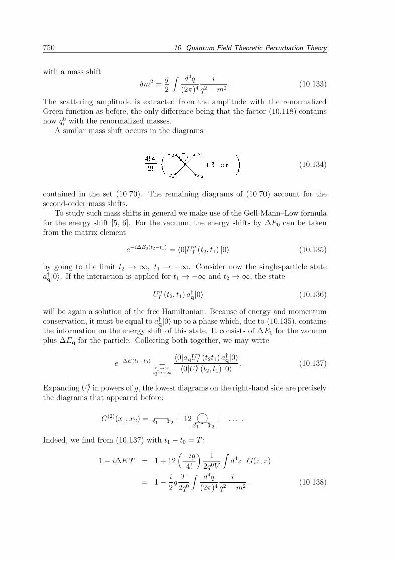
A similar mass shift occurs in the diagrams
(10.134)
contained in the set (10.70). The remaining diagrams of (10.70) account for thesecond-order mass shifts.
To study such mass shifts in general we make use of the Gell-Mann–Low formulafor the energy shift [5, 6]. For the vacuum, the energy shifts by ∆E0 can be takenfrom the matrix element
e−i∆E0(t2−t1) = 〈0|UηI (t2, t1) |0〉 (10.135)
by going to the limit t2 → ∞, t1 → −∞. Consider now the single-particle statea†q|0〉. If the interaction is applied for t1 → −∞ and t2 → ∞, the state
UηI (t2, t1) a
†q|0〉 (10.136)
will be again a solution of the free Hamiltonian. Because of energy and momentumconservation, it must be equal to a†q|0〉 up to a phase which, due to (10.135), containsthe information on the energy shift of this state. It consists of ∆E0 for the vacuumplus ∆Eq for the particle. Collecting both together, we may write
e−∆E(t1−t0) =t1→∞
t2→−∞
〈0|aqUηI (t2t1) a
†q|0〉
〈0|UηI (t2, t1) |0〉
. (10.137)
Expanding UηI in powers of g, the lowest diagrams on the right-hand side are precisely
the diagrams that appeared before:
G(2)(x1, x2) = q qx1 x2
+ 12 ♥q qx1 x2
q + . . . .
Indeed, we find from (10.137) with t1 − t0 = T :
1− i∆E T = 1 + 12(−ig
4!
)
1
2q0V
∫
d4z G(z, z)
= 1− i
2gT
2q0
∫
d4q
(2π)4i
q2 −m2. (10.138)
10.8 Wick Rules for Scattering Amplitudes 751
Similarly, we may use formulas (10.106), (10.107), and the energy shifts q0 → q0 +∆E = q0R, to write
a†q = limx0→−∞
√
2q0RV
∫
d3x ei(q0
Rx0−qx)φ(x), (10.139)
aq = limx0→∞
√
2q0RV
∫
d3x e−i(q0Rx0−qx)φ(x). (10.140)
Now every particle line automatically receives a factor ei∆EqT , which removes pre-cisely the phase factor (10.135).
To higher orders in g, it is somewhat hard to proceed in this fashion. Theproblem will be solved in the next section with more elegance.
Note that formula (10.137) allows us to evaluate the shift in the particle massin another way. If q0 =
√q2 +m2 is the energy before turning on the interaction,
then
q0 +∆E =√
q2 +m2 + δm2 = q0 +δm2
2q0(10.141)
is the energy afterwards, and we find once more the mass shift (10.133).
10.8 Wick Rules for Scattering Amplitudes
The possibilityX of obtaining external particle states from fields with the help oftemporal limiting procedures of the type (10.107) allows us to incorporate the cre-ation and annihilation operators of these particles into the general framework ofWick’s contraction rules. Confronted with the numerator of the perturbative scat-tering amplitude in (10.103),
SN (q4q3|q1q2) ≡ 〈0|aq4aq3
Te−i∫
∞
−∞dtVI (t)a†q2
a†q1|0〉, (10.142)
we may imagine the incoming particle operators on the one side to carry negativeinfinite time arguments, and the outgoing ones on the other side to carry positiveinfinite times. Then they can be brought inside the parentheses of the time-orderingoperator. This, in turn, can be evaluated as usual via Wick contractions.
The results of the last section show that the Wick contractions leading to anexternal particles are
φ(x)a†p = [φ(x),a†p] =1
√
2V ωp
e−iqx, (10.143)
apφ(x) = [ap,φ(x)] =1
√
2V ωp
e−iqx, (10.144)
752 10 Quantum Field Theoretic Perturbation Theory
where ωp =√p+M2.
For Dirac particles, there are the corresponding contraction rules
ψ(x)a†p,s3 = φ(x),a†p =1
√
V Ep
u(p, s3)e−ipx, (10.145)
ap,s3ψ(x) = ap,s3,ψ(x) =1
√
V Ep
eipxu(p, s3), (10.146)
and for antiparticles:
ψ(x)b†p,s3 = φ(x),b†p =1
√
V Ep
e−ipxv(p, s3), (10.147)
bp,s3ψ(x) = ap,s3,ψ(x) =1
√
V Ep
v(p, s3)eipx, (10.148)
where Ep ≡√p+M2.
10.9 Thermal Perturbation Theory
Since Wick’s theorem was valid for thermal Green functions, we expect all pertur-bation expansions to have a simple generalization to the thermal case. Let us definea thermal Heisenberg picture for operators by
OH(τ) = eHτ/hOSe−Hτ/h, (10.149)
and an interaction picture which moves according to the free equations of motion,
OI(τ) = eH0Gτ/hOSe−H0Gτ/h. (10.150)
Thus, a Heisenberg operator can be transformed to the free operator via
OH(τ) = UI(0, τ)OI(τ)UI(τ, 0) (10.151)
where
UI(τ2, τ1) = eH0Gτ2/he−HG(τ2−τ1)e−H0Gτ1/h (10.152)
is the time displacement operator along the euclidean time axis τ . Therefore it hasthe same factorization property as the quantum mechanical operator UI(t2, t1) inEq. (9.17):
UI(τ3, τ2)UI(τ2, τ1) = UI(τ3, τ1). (10.153)
10.9 Thermal Perturbation Theory 753
Certainly
UI(τ1, τ1) = 1. (10.154)
However, in contrast to UI(t2, t1), this operator does not satisfy the unitarity relation(9.26), but instead:
UI(τ2, τ1)† = UI(−τ1,−τ2). (10.155)
It obeys the following equation of motion
h∂τUI(τ, τ′) = eH0τ/h (H0G −HG) e
−HG(τ−τ)/he−H0Gτ/h
= −VI(τ)UI(τ, τ′), (10.156)
where VI(τ) is the time-dependent thermal interaction picture of the time indepen-dent Schrodinger perturbation V = VS
VI(τ) = eH0Gτ/hV e−H0Gτ/h. (10.157)
Therefore we can solve (10.156) for UI(τ, τ′) using the standard exponential
Neumann-Liouville expansion (9.19), now time-ordered with respect to the euclideantime τ :
UI(τ, τ′) =
∞∑
n=0
(
−1
h
)n 1
n!
∫ τ
τ ′dτ1
∫ τ
τ ′dτ2 . . .
∫ τ
τ ′dτnTT [VI(τ1) · · ·VI(τn)]
= Tτe− 1
h
∫ τ
τ ′dτ ′′VI (τ
′′). (10.158)
By construction, UI(τ, 0) satisfies the relation
e−HGτ/h = e−H0τ/hUI(τ, 0). (10.159)
Thus, using the thermal value for the imaginary time τ/h = 1/kBT ≡ β, we obtaindirectly a perturbation expansion of the partition function
Z = Tr(
e−βHG
)
= Tr[
e−βH0GUI (β, 0)]
(10.160)
=∞∑
n=0
(
−1
h
)n 1
n!
∫ β
0dτ1 · · ·
∫ β
0dτnTr
[
e−βH0GTτ (VI(τ1) · · ·VI(τn))]
.
Consider now a thermal two-body Green function in the presence of interaction,defined for τ > τ ′ as follows:
G(x, τ ;x′, τ ′) ≡ Tr[
e−βHGψ(x, τ)ψ†(x′, τ ′)]
/Tr(
e−βHG
)
= Tr[
e−βH0GUI (β, 0)UI(0, τ)ψI(x, τ)UI(τ, 0) (10.161)
× UI(0, τ′)ψ†
I(x′, τ ′)UI(τ
′, 0)]
/Tr[
e−βH0GUI (β, 0)]
.
754 10 Quantum Field Theoretic Perturbation Theory
For τ < τ ′, on the other hand, we have
G(x, τ ;x′, τ ′) ≡ ±Tr[
e−βHGψ†(x′, τ ′)ψ(x, τ)]
/Tr(
e−βHG
)
= Tr[
e−βH0GUI (0, τ′)ψ†
I(x′, τ ′)UI(τ
′, 0) (10.162)
× UI(0, τ)ψI(x, τ)UI(τ, 0)] /Tr[
e−βH0GUI (β, 0)]
.
Both equations may be combined in the single formula
G(x, τ ;x′, τ ′) = Tr[
e−βH0GTτUI (β, 0)ψ(x, τ)ψ† (x′, τ ′)
]
/Tr[
e−βH0GUI (β, 0)]
.
(10.163)
In comparison with the field theoretic formulas (10.9) and (10.12), the vacuum ex-pectation values are replaced by the Boltzmann-weighted thermal traces, and thevacuum expectation value of the S matrix operator UI (∞,−∞) in the denom-inators is replaced by the Boltzmann-weighted trace of the interaction operatorUI (h/kBT , 0) along the euclidean time axis τ .
Note that the denominator ensures the existence of the zero temperature limitin just the same way as the phase factor did in the switching-on limit η → 0. Infact, the grand canonical partition function in the denominator may be written as
ZG = eβΩ =∑
n
e−(βEn−µNn), (10.164)
such that the limit T → 0 renders a pure exponential with the ground state energy
ZG →T→0
e−β(E0−µN0) → e±∞. (10.165)
This is the analogue of the infinite phase factor for the field theoretic denominatorin Eq. (10.9).
Let us now expand the interaction operator UI (h/kBT , 0) in powers of the in-teraction, just as before in real time. This leads to a series of thermally aver-aged products of many fields ψI(x, τ) which move according to the free field equa-tions. Therefore Wick’s theorem can be applied and we obtain an expansion ofG(x, τ ;x′, τ ′) completely analogous to the field theoretic one. The only differenceis the finite-time interaction. When going to Fourier transformed space, the finiteeuclidean time interval is fully taken into account by the sum over the discreteimaginary Matsubara frequencies.
We have seen before that the evaluation of field-theoretic Green functions pro-ceeds best via a Wick rotation of the energy in the perturbative digrams to animaginary axis. This is precisely the axis along which the Matsubara frequenciesare situated. Thus, as far as perturbation theory in Fourier transformed space isconcerned, the diagrammatic rules are exactly the same, except that the Wick ro-tated integrals over the imaginary energy have to be replaced by the Matsubarafrequency sums [recall Eq. (2.415)]:
∫ dp0
2π→ i
∫ ∞
−∞
dpE2π
→ kBT
h
∑
ωm
=1
β
∑
ωm
, ωm=2π
hβ
m for bosons,m+ 1
2for fermions.
(10.166)
Notes and References 755
In the limit of small temperatures, the Matsubara frequencies move closer and closerto each other, and sums over them tend to frequency integrals.
The two descriptions coincide, apart from the trivial presence of the chemicalpotential in the grand canonical energy. We conclude that the Wick-rotated calcula-tion of field theoretic Green functions really amounts to thermal equilibrium physicsin the limit of zero temperature.
Let us point out that the result (10.163) implies the same periodicity in h/kBT =β of the full Green functionG(x, τ ;x′, τ ′) as in the free case (2.413). First, we observethat due to the time independence of the Hamiltonian, there is now translationalinvariance in euclidean time T such that G(x, τ ;x′, τ ′) depends only on the differenceτ − τ ′:
G(x, τ ;x′, τ ′) =Tr[
e−HG(β− τh)ψ(x, 0)e−HG
τ−τ ′
h ψ†(x′, 0)e−HGτ ′/h]
/ Tr(e−βHG)
=Tr[
e−HG(β− τh)ψ(x, 0)e−HGτ−τ ′/hψ†(x′, 0)
]
/Tr(e−βHG). (10.167)
Similarly, we conclude the dependence only on x− x′ by translational invariance inspace, using ψ (x, τ) = eiPx/hψ(0, τ)e−iPx/h with the momentum operator P. Thuswe may write
G(x, τ ;x′, τ ′) = G(x− x′, τ − τ ′), (10.168)
just as for the field theoretic Green functions in the vacuum. Now it is easy to seethe periodicity. For the interval τ − τ ′ ∈ (−h/kBT , 0) we calculate
G (x− x′, τ − τ ′) = ±Tr[
e−βHGψ†(x′, τ ′)ψ(x, τ)]
/Tr(e−βHG)
= ±Tr[
ψ(x, τ)e−βHGψ†(x′, τ ′)]
/Tr(e−βHG)
= ±Tr[
e−βHGψ (x, τ + β)ψ†(x′, τ ′)]
/Tr(e−βHG)
= ±G (x− x′, τ − τ ′ + β) , (10.169)
thus showing that interacting Boson and Fermion thermal Green functions are pe-riodic and antiperiodic under the replacement τ → τ + β, just as in the free case inEq. (2.413).
Notes and References
[1] R.P. Feynman, Phys. Rev. 91, 1291 (1953); G.V. Chester, Phys. Rev. 93, 1412 (1954).
[2] S. Schweber, Relativistic Quantum Fields , Harper and Row, N.Y., 1961.
[3] M.E. Peskin and D.V. Schroeder, Introduction to Quantum Field Theory, Addison-Wesley,Reading, MA, 1995.
[4] H. Kleinert and V. Schulte-Frohlinde, Critical Properties of φ4-Theories , World Scientific,Singapore 2001, pp. 1–489 (http://klnrt.de/b8).
[5] M. Gell-Mann and F. Low, Phys. Rev. 84, 350 (1951).
756 10 Quantum Field Theoretic Perturbation Theory
[6] M. Gell-Mann and M.L. Goldberger, Phys. Rev. 91, 398 (1953).
[7] H. Kleinert, Gauge Fields in Condensed Matter , World Scientific, 1989, pp. 1–744 (kl/b1).
[8] H. Kleinert, in Proceedings of a NATO Advanced Study Institute on Formation and Inter-
actions of Topological Defects at the University of Cambridge, England, A.C. Davis and R.Brandenberger, eds., Kluwer, London, 1995 (kl/227).
[9] H. Kleinert, Multivalued Fields , World Scientific, Singapore 2008, pp. 1–497 (kl/b11).
[10] C. Schubert, Perturbative Quantum Field Theory in the String-Inspired Formalism, Phys.Rept. 355, 73, (2001) (arXiv:hep-th/0101036).
[11] See for instance Chapter 7 in the textbookS. Gasiorowicz, Elementary Particle Physics, John Wiley, New York, 1955.