WORKING PAPERS

PROCESS ANALYSIS, CAPITAL UTILIZATION, AND

THE EXISTENCE OF DUAL COST AND PRODUCTION FUNCTIONS*

Christopher C. Klein

WORKING PAPER NO. 116

May 1984

Fl'C Bureau of Economics working papers are preliminary materials circulated to stimulate discussion and critical comment All data contained in them are in the public domain. This includes information obtained by the Commission which has become part of public record. The analyses and conclusions set forth are those of the authors and do not necessarily reflect the views of other members of the Bureau of Economics, other Commission staff, or the Commission itself. Upon request, single copies of the paper will be provided. References in publications to FfC Bureau of Economics working papers by FfC economists (other than acknowledgement by a writer that he has access to such unpublished materials) should be cleared with the author to protect the tentative character of these papers.

BUREAU OF ECONOMICS FEDERAL TRADE COMMISSION

WASHINGTON, DC 20580

EX ISTENCE

PROCESS ANALYSIS, CAP ITA L UTI L IZATION, AND

THE OF DUAL COST AN D PRODUCTION FUNCTIONS*

Christop her c. Klein

Federal Trade Commission

Bureau of

Was hington,

March 1984

Economics

D. C. 20580

* Thanks are due to Knox Lovell, John Stewart, Helen. Tauchen, and, especially, Nicholas Georgescu-Roegen for their invaluable comments. The views expressed here are those of the author alone and do not represent those of the Federal Trade Commission.

I. Introduction

This paper integrates the literature on capital utilization

and shiftwork with the duality theory of cost and production

functions. The model constructed below posits a production

technology consisting of an instantaneous rate of production

function and a time duration variable. The existence of a cost

function dual to this tec hnology then follow9 directly from

assumptions on the mathematical properties of the rate function.

Marris's (1964) original work on the economics of capital

utilization, and the more recent contributions of Betancourt and

Clague (1981), and Winston (1982) either ignore or are outright

hostile toward duality theory. The·time utilization of plant and

equipment embodied in these models, however, is not inconsistent

with the mathematical methods used in the "timeless'' duality

theory. Indeed, the model proposed here contains neoclassical

duality theory as a special cas .

The crucial tool in this construction is Georgescu-Roegen 's

(1970, 1971, 1972) process analysis of production. His analysis

of an idealized factory yields a production model that precisely

specifies the inputs and initially recognizes the time duration of

production. Thus, the production process is directly modeled,

rather than abstractly constructed. In this way the model is

similar to engineering approaches to production. l

The interesting aspects of the model, however, derive not

from the process analysis, but from the speci fication of input

prices. The· time element enters the cost function because the

input prices must account for the time use of the inputs. Time

affects the cost of labor directly, while the purchase price of

capital is generally invariant wit h respect to production time.

This asymmetry in the behavior of input prices over time combined

with the returns to scale characteristics of the rate function

determine the cost minimizing length of the "working day".

For the sake of argument, the term "neoclassical" is used to

denote the class of production models whic h ignore the firm's

c hoice of the working day. These models treat inputs as flows

accumulated over a fixed period of time with fixed (time

invariant) prices. Recent theory has employed these models to

such an extent that Winston criticizes them under the heading of

duality models. Nevertheless, the objectionable assumptions

underlying this literature can be traced to Wicksteed's pioneering

work in the Nineteenth Century. 2 Thus, neoclassical is used here,

however unfairly, to characterize a diverse literature in

production theory. 3

Fortunately, the mathematics behind duality approaches to

production are blissfully indifferent to the meanings we attac h to

them. 4 This allows us to

results

apply familiar mat hematical concepts to

a novel production tec hnology with relative ease. In fact, it is

possible to derive obtained by Winston, and by Betancourt

and Clague for linearly homogeneous production functions and

extend them to the class of homothetic production functions.

For purposes of exposition, the model is built in reference

to a working day. This is not a prerequisite. The time period to

-2­

Factory Analysis

be determined can be structured in any number of ways. Daily pro­

duction, however, is immediately applicable to questions of

capital utilization and shiftwork on which the existing literature

has focused.

The process analysis of factory production is reviewed in the

following section. Section III establishes the cost function dual

to the production tec hnology of sect.ion II, and demonstrates some

grap hical properties of the model using familiar isoquant

concepts. Section IV extends the model to include time variable

prices and a sloped output demand curve in the context of profit

ma ximization. Section V examines the characteristics of the

optimum length of the working day and section VI concludes the

investigation.

I I. Production: A Process View

Suppose we wish to analyze the production process of an

industrial factory. By the term factory is meant an assembly line

or "in line" process as opposed to an "in parallel" process suc h

as agriculture. In an assembly line factory there are a succes­

sion of work stations suc h that at any given time there is a

potential unit of output in each work station. Furt hermore, each

worker and each article of capital are continuously employed by

switching to a new unit of output as soon as their task on the

previous unit has been completed. What we observe is a continuous

line of "goods in process" moving successively from work station

to work station until exiting the process as finis hed goods.

-3-

The process analysis of a factory begins by surrounding the

factory wit h an analytical boundary. This boundary is an

imaginary barrier placed around the factory at the discretion of

the investigator in order to separate the process to be observed

from the rest of the world. The investigator may also choose the

placement of this boundary as it best suits the goals of the

analysis. Let us .choose our analytical boundary suc h that all raw

materials, energy, and previously processed (i. e. , intermediate)

inputs must move across this boundary directly into the factory

process, and all outputs cross the boundary immediately upon exit

from the process. This has been done schematically in Figure 1.

We can observe that at any moment there is some flow of

inputs across the boundary and some associated flow of output and

"waste products" across the boundary in the opposite direct ion.

We also observe some factors of production present inside the

boundary whenever the factory is· in operation. 1'hese factors are

what we commonly think of as labor and capital, plus the goods in

process present at each work station along the assembly line.

Thus the flow of output produced is related to the flow of

material and energy inputs and the "quantity" of labor and capital

present at the time. In mathematical notation

(1) q('t') f(K(T), H(T), X('t')) =

says that the maximum rate at which output crosses the process

boundary at time T, q(T), is a function of the capital K and labor

H present at T, and the rate x at which ot her inputs enter the

-4-

.

Capital

7

. I .

I

I

I

I

raw materials

energy

intermediate goods

(K) land stru ctures machines tools etc.

Labor (H)

skilled workers unskilled workers supervisors etc •

Analytical Boundary

product

waste

Fig. 1. Process Analysis of a Factory

process at time T. Notice that q can be a vector of output rates,

excluding the residual waste products, for the case of joint

saleable outputs; that K is a census of mac hines and structures of

each types present at T; that H is a census of workers of each

type present at T; and x is a vector of input flow rates at time

T.

If T is the period over which the factory operates, then

total production is given by

T ( 2) Q = J0

f ( K (T), H (T),x (T))dT.

If the capital and labor present over the period and the flow

rates of inputs are constant, and the productivities of the

factors are not affected by the length of the period, we can

simplify (2) to

(3) Q T•f (K, H, x). =

This says that the total output of the factory is determined by

the length of time the factory operates T, the capital and labor

on hand over the period, and the flow of ot her inputs over the

period. In addition (3) indicates that in order to produce the

quantity Q of product the firm must choose the capital and labor

to hire, the flow of inputs to purchase, and the length of the

period to operate, T. Therefore the process analysis of factory

production provides us wit h a production model that therequ·ires

- 6 -

model

among

fund

actually

process

firm to choose input factor proportions as well as a time period

of operation in order to produce the desired output quantity Q.

Equation (3) also shows an unf amiliar relation between the

input factors and the quantity of output. K and H are just

numbers of men and machines independent of time, while x is a

vector of flow rates, or quantities per unit time. The first to

develop a accounting for, and elaborating on, the

differences capital , labor, and flow inputs was Nicholas

Georgescu-Roegen (1971). He denoted the capital-· .

and labor

components of (3) by the and the material and

energy inputs by the term derivation of the

flow factor's nomenclature is fairly obvious from (3) since the

flow factors appear as flows in the function f. The case for the

factors is not, in comparison, clear.

Georgescu-Roegen reasons that the stock of capital inputs is

a stock of machines that is perpetually maintained by the

in which it participates. This stock

represents the available capital services the firm buys when it

purc hases a machine, or a whole plant, where the actual amount of

capital services used is measured as machine hours for each type

of machine. This "is less misleading than talking of service

stocks because there is no physical flow that augments or depletes

the capital fund. In fact, the capital fund can only be drawn

down by running the machine until it is no longer economically

feasible to do so. One cannot consume the entire ·fund immediately

nor stretch the fund over a longer period by feedi ng in new

term fund factors

flow factors. The

-7­

supplies of services. Regular maintenance must be undertaken to

insure eac h mac hine's operating efficiency, of course, but this

does not increase the fund represented by a machine. At some

point the machine will become very expensive to maintain, at which

time it will be scrapped.

There are two ma jor characteristics of a fund factor of

production that we can identify :

1. The fund factors are not quantitatively altered by the

production process.

2. A period of time is required to exhaust the services

represented by a fund factor.

It is obvious that the capital and labor elements of (3)

represent fund factors in the factory process. Moreover, it is

the of fund service that appears in (3) and is denoted by K

and H. This can be illustrated wit h a simple example. Suppose a

factory employs 50 wor kers for a period of 10 hours. The quantity

of labor services used over the period is given by (50 men)•(lO

hours) = 500 manhours. The rate of service use is then the

quantity of labor services used divided by the period of time over

which the services are rendered, or (500 manhours)/ (10 hours) = 50

men. The rate of fund service is just the number of each fund

factor present at any time the factory is in operation.

Now reconsider the right hand side of (3). Since K and H are

the census figures for machines and workers present while the

factory operates, they are the number of each type of fund factor

therefore they represent the rates of fund service. Inpresent,

-8-

addition, the vector x represents the observed rates of flow of

material and energy inputs into the process. This indicates that

the function f(K, H, x) relates the rate at whic h output is

produced to the rates at which input factors are used (as in

(1) ) •

It may be instructive to consider two comments on factory

processes. The first is by Georgescu-Roegen as he explains the

fund factors participation in the process, " • • • in the case of

manufactured or mi ned products, we can arrange the elementary

processes in line in such a manner that each fund shifts to

another process as soon as it has finished its task in the

previous one. This is how any factory operates, like an assembly

line even though orie is not in direct view. "S A similar point has

been mentioned by Marsden, Pingry, and Whinston, "• • • an

assembly plant could be characterized by a series of assembly

units (reactors), and the process could be described in terms of a

rate equation. " 6 This is precisely what equation (1) and its

counterpart equation (3) attempt for a factory process. The rate

of output is determined by a function of input rates, and the

total quantity is found by multiplying the rate of output by the

time period T.

Georgescu-Roegen spent a great deal of time formulating

the substitution relationships among the inputs so that their

co mpliance with the physicists' principle of Conservation of

Matter-Energy was clear. This expanded the number and complexity

of the structural equations and emp hasized the unusual aspects of

-9­

it

the flow-fund approach. While his treatment of the waste outputs

and the relation of the inputs and outputs to plant capacity was

uniquely insightful, it undermined the intuitive appeal and the

empirical utility of his production model.

Fortunately it is possible to construct a model in the spirit

of Georgescu-Roegen that can be represented more simply. Equation

(3) and a dose of Alfred Mars hall's "sensitiveness of touch" are

the main ingredients. The primary diff iculty is in understanding

the way in which substitution occurs between the flow and fund

factors and its relation to the conservation principle. Examine

equation (2) once again

q f(K, H, x). =

By the conservation principle we know that in matter-energy

terms the flow inputs must equal the flow outputs. Suppose we

define q to be only the product flow, or a restricted output

vector that excludes the waste products. If we are given (2) and

some values K, H, and x, we can find q. We can then calculate

the "waste" output from q and x : w [x-q] . Since we can never=

observe a process that defeats the conservation principle, it is

not necessary to carry as an explicit constraint. We can

presume that any process_we might meet obeys all physical law s and

subsume these implicitly in the f function.

There are several advantages to this approach. First, this

allows the rate function f to display all the usual substitu­

tability properties we are accustomed to, except in terms of rates

-10­

Duality

• •

III. In the Flow-Fund Production Model

Suppose we have an N factor neoclassical

instead of quantities as in the strict neoclassical world. If we

wish to increase the rate of output of the product by hiring more

labor but no more material inputs, then this requires that the

additional labor alter the relative amount of waste product flows.

If the waste flow is not altered then the rate of product flow

will not change, but the f function still gives us a maximum

output rate q for any values of K, H, and x.

Furthermore, we can define the "product" an<i the "waste"

outputs by letting q be the outputs wit h positive prices. The

waste products are then identified as the residuals.

In sum mary, we have a production model in (2) and (3) that

gives the rate of output as a function of rates of input flows and

rates of fund service. This model allows sub stitution among the

inputs similar to the usual neoclassical production function,

while incorporating the strengths of the flow-fund model.

production function

F : u = F(yl, Y2, • , YN) F(y) where u is the· amount of output =

produced during a given period of time and y = (yl, • • , YN) ) O N•

is a nonnegative vector of input quantities used during the

period. Suppose also that the producer faces fixed positive

prices for inputs (pl, P2, • • • , PN) = p and that the producer does

not possess market power in the input markets.

-11­

Assumption

Properties

linearly homogeneous

We now define the producer's function C as the solution

to the problem of mi nimizing the cost of producing at least output

level u, given the input prices p, or

(4) C(u, p) miny {p'y : F(y) ) u } •=

Assumption 1 below is sufficient to imply the existence of

solutions to the cost minimization problem as stated in the lemma

that follows.

1 : F is continuous from above; i. e. , for every u €

range F, L(u) = {y : y ) O N, F(y) ) u } is a closed set.

L emma 1 : If F satisfies Assumption 1 wit h p >> ON, then for

every u € range F, miny { p'y : F(y) ) u } exists.

Furthermore the following seven properties ca n be derived for

the cost function C requiring only Assumption 1 on F.

I for C :

Cl : C is a non-negative function; i. e. , for every u € range F and

p >> ON, C ( u , p ) ) 0 •

C2 : C is (positively) in input prices

for any fixed level of output; i. e. , for every u €

range F, if p >> ON and k > 0, then C(u, kp) = kC (u, p).

C3 : If any combination of input prices increases, then the

minimum cost of producing any feasible output level u

will not decrease; i. e. , if u € range F and Pl ) POr

then C(u, Pl) ) C(u, po).

-12­

non-decreasing

Lemma

p *) •

C4: For every

range F, C(u, p) is continuous in p,

is in u for fixed p;

u E range F, C(u, p) is a concave function of p.

CS: For u E p > > ON•

C6: C(u, p) i. e. , if

p >> ON, uo, Ul E range F and uo Ul, then C(uo, p) C(ul, p) .

C7: For every p > > ON, C(u, p) is continuous from below in u;

i. e. if p* > > ON, u* E range F, un E range F for n 1, 2, =

. . . , Ul u2 ••• and lim Un = u*, then limnC(un,p) = C(u*,

These results are well known and the proofs can be found in

numerous places. We have followed Diewert's (19 82) rendition of

the standard duality results above and follow his work once again

in stating the ne xt result, frequently called Shep hard's Lemma.

2: 'I f the cost function satisfies Properties

input prices

I for C and,

in addition, is di fferentiable with respect to at the

point (u*, p*) , then

(5 ) y ( u *, p*) Vp C ( u *, p*)=

where y(u*, p*) = [yl(u*, p*) , •••, YN(u*, p*) ]' is the vector of

cost minimizing input quantities needed to produce u* unit s of

output given input prices p*, where the underlying production

function F is defined above, u* E range F and p* >> ON•

The advantage of using Lemma 2 is that only the cost function

is req uired to have certain properties and the corresponding

production function F is derived from the given cost function.

Given a cost function satisfying Properties I, we can derive the

-13­

(7)

input demand equations directly from the functional form of C. It

is not necessary to find F nor to carry through the entire

constrained maximization of the production function explicitly to

find the input demand equations.

Now suppose we have the production rate function below:

(6) q = f(K, H, x) .

where q is the ma ximum quantity produced by continuous operation

of a factory at a constant instantaneous rate for a 24 hour

period; K is the rate of capital fund service over the period, or

the number of ma chines and structures present over the period,

assumed constant for any "day"; H is the rate of fund ser vice for

labor, or the number or wor kers of each type present at any time

during the period; and x is the quantity of material inputs used

for a constant instantaneous rate of input flow sustained for a 24

hour period.

Notice that equation (6) describes a production tec hnology

commensurate wit h the neoclassical production function when the

given period of time is 24 hours and the measurement of labor and

capital inputs is specified more precisely. However, the quantity

produced in a working day is given by·

Q = t • f(K, H, x) , 0 < t <: 1

where t is the utilization rate, or proportion of a 24 hour period

that the factory is in operation, and it follow s that Q = tq.

-14­

Since a dual cost function must· exist for f in (6) with given

input prices by Lemma 1, a cost function dual to (7) should also

exist, but it will not be identical to the neoclassical cost func­

tion due to the institutional differences in payments to ca pital

vs. the other inputs. We take account of the firm's ability to

purc hase labor services and material input flow s, but only the

capital fund in the definition of the flow-fund cost function

( 8) C0(0, t, p) - min { pkK + tphH + tpxx : tf (K,H, x) ;> 0 } K,H,x

or equivalently

(9) C(q, P) - min { pkK + tphH + tpxx : f( K, H, x) ;> q, K,H,x

tq = 0 }

where

for any

where 0 =

P is the modified input price vector, P - (pk,tPhrtPx) . 7

Since given value of t, tf (K, H, x) ;> Q implies f(K, H, x)

;> q tq by definition, the two forms of cost (8) and (9)

are identical for any quantity O, and given values for t and input

prices p.

The equivalence of (8) and (9) causes some difficulties in

notation when the derivatives of C and co with respect to q and t

are encountered. Since this .occurs repeately, the following con­

ventions in notation are followed:

=cq ac;aq = dC0/dq p =po t=to

aco;ao (30/aq) = (ac;ao) t

(10)

Ct = ac;at = dC0/dt I = aco;ao (3Q/3t) + aco;at q=qo

-15­

The usual notation for a partial derivative is used throug hout.

Note that prices are not required to remain fixed for Ct since we

will presently allow some prices to change with utilization rate.

We interpret Cq and Ct as the marginal cost of increasing output

by increasing rate of production and the ma rginal cost of

increasing output by increasing utilization rate, respectively.

Recall that the input prices in (8) - (10) are daily prices,

or prices per 24 hours. This means that Pk is depreciation and

interest for one day; Ph is the cost of employing one worker for

24 hours, or Ph = 24wh where wh is the hourly wage; and Px is just

the price per unit of the flow inputs.

Suppose that C and co have properties I for C, so that

factor demand equations can be found by Lemma 2. Suppose further

that C(q, P) is twice continuously differentiable at the point

(q*, P*) . Then differentiating (9) with respect to factor prices

gives daily factor dema nd functions

ac;apk = K(q*, P*) , ac;aph = tH (q*, P*) ,

(11)

ac;apx = tx(q*, P*) .

Further, we know the following so-called sym metry conditions must

holds

-16­

But here is a surprise. For the labor and flow inputs we get the

usual result

while for the capital input we find

i. e. , the usual conditions are now weig hted by the utilization

rate t. Georgescu-Roegen (1972) derives an equivalent result

using the Lagrangean method: that the marginal rate of substitu­

tion of capital for labor is equal to the price ratio weig hted by

the utilization rate. He interprets this to mean that the budget

line in K and H space is not tangent to the relevant isoquant when

t < 1. We know that this is not possible for a (K, H) co mbination

that is a solution to the cost minim ization problem. A closer

look at (14) resolves this parado x.

Recall, first of all, that Ph is defined as a

for labor, Ph 24wh when wh is the hourly wage. This

daily price

means=

changes in Ph arise from changes in wh alone, or

And using this with (14) yields

which we rea rrange to find

=(17) 3K/3w h 24t(3H/3pk) T(3H/3pk) 3(TH) /3Pkr= =

-17­

where T is the number of hours per day that the factory operates.

Of course TH is nothing more than the number of ma nhours, or the

quantity of labor services, used by the firm in a working day. We

can now write the demand for labor services as

(18) M(T, q, P) = T•H(q, ),

and this allow s us to rew rite (14) in the more familar form

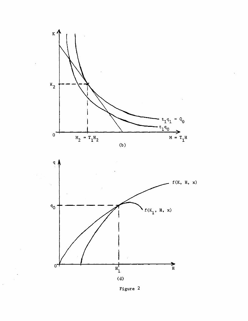
Clearly the relevant isoquant is in K and M = TH space as

shown in Fig. 2 (a) . Furthermore, the isoquants contain both a

production rate and a utilization rate component, Q = t·q. In

2 (a) the isoq uant is drawn for a fixed utilization rate to, and

the labor services determined by the tangency imply some number of

wor kers, Hl, for the entire working day, To = 24to, so M1 = ToHl•

If we wish to consider utilization rates other than to, it

is necessary to redraw the isoquant map for the new t. This has

been done in Fig. 2(b) for t1 < to. Reducing the length of the

working day from To to T1 shifts the isoquants so that the firm

moves to a hig her rate q1 to maintain output at Oo. Figure 2(c)

shows this change in the utilization rate in K and H space. Here

the fall in the length of the working day appears as a fall in the

"price," or relative daily cost, of a worker which rotates the

budget line away from the H axis. The firm reacts to this change

as it would to a change in the wage, by substituting labor for

-18­

�--------�------�------------�

-· .

K

0 M = T H.

0 (a)

K

0 H

Figure 2

K

0 M = T H1

(b)

f(K, H, x)

q

0 H

Figure 2

Output Input

cap ital and moving to a higher rate of production. We can see

that the deciding factor for the firm is no longer the relative

pri ces of the inputs, but the relative daily cost of the inputs

when the lengt h of the working day is a decision variable.

Suppose the producer chooses production rate qo and hires K1

and H1. This represents only one point on the plant's planning,

or long run, production rate function f(K, H, x) . The producer is

free to vary his labor and flow inputs on a daily basis so he has

the short run production rate function f( Kl, H, x) shown in Fig.

2 (d) . The firm is always able to move along f( K, H, x) at any

time, but can forego the cost of rea rranging its capital from day

to day by moving along f( Kl, H, x) as dem and fluctuates. Now we

may observe the firm adj usting its input mi x as well as the length

of the working day in response to short run fluctuations.

IV.

Two obvious extensions of the model involve the usual

"monopoly problem" , in which the firm faces a sloped demand curve,

and the case of input prices that va ry with the utilization rate.

The derivations of both of these are based on Diewert (1982) ,

where the case of a variable input price is formally a modifica­

tion of the monoposony problem. This section derives the flow­

fund equivalents of the neoclassical duality results.

Suppose we have a flow-fund production function f that

satisfies the following conditions:

Variable and Prices

-21­

increasing.

quasiconcave

(i) f is a real valued function defined over the non-

and continuous

a

negative orthant on this domain.

(ii) f is

(iii) f is function.

then given f and positive inputs and outputs, we write the

profit maximization problem as

(20) max { D(Q) Q - C(q, P) Q = tq > 0, 0 < t ( 1} t,q

= D(Q*) Q* - C(q*, P*).

Q is total daily output, D(Q) is a daily inverse demand function,

and C(q, P,) is the cost function dual to f. Solutions to the

profit maximization problem are denoted by an asterisk. The first

order conditions for a ma ximum are

D(Q) q + (aDjaQ) qQ - Ct = 0 ( 21)

=D(Q) t + (aDjaQ) tQ - Cq 0

where Cq and Ct are defined by (1 0). This condition can be

restated as

= =(22) Cq/t MR Ct/q

where MR is marginal revenue in the usual sense. This condition

can be interpreted as a variant of the typical neoclassical

marginal condition: the firm chooses to operate where the marginal

gain from an increment to time in production is just equal to the

marginal gain from an increment to rate of production. Cq/t and

-22­

Ct/q are "marginal cost" in the two output dimensions weighted

by the reciprocals of t and q. Thus "marginal revenue equals

marginal cost" in (30).

Input prices that va ry by "time of day" can be incorporated

in this framework, if the utilization rate can be measured

relative to a specific starting time during the day. The proper

measurement of t will guarantee that the size of t corresponds to

a known set of operating hours such that t and "time of day" are

paired. In this context input prices that change over the course

of the day can be desc ribed by a price function P, P(t) > 0, that

depends on utilization rate.

Applying Diewert's (1982) treatment of the monopoly and

monopsony problems for econometric purposes, if we know the ou tput

demand function and the input price or supply func tions, then the

system defined by (21) is identical to the profit function dual to

f when the output and input prices have been "linearized" as thei r

shadow prices. That is, for example, if

=Pq D(Q) + [aD (Q) jaQ] Q P; + D' (Q) Q, =

is the shadow or marginal price of output, where P* is theQ

product price, then

maxq,t {pqO - P'X : Q tq > 0, 0 < t(l} = IT(pq,P ) =

where IT is the firm's true profit function which is dual to the

rate function f. 9

-23­

( /2 4 )

V. Restrictions on the Production and Cost Functions

We can now make some statements on the firm's optimal choice

of q and t by im posing restrictions on the form of f, which imply

a form for C. Suppose f is homogeneous of degree l/ 8 suc h that

(23) f(X) = [g (X) ] l/ 8

where g(X) is linearly homogeneous. Then

f (>.X) = >.l/ 8 f(X) = [g (>.X) ]l/ 8 = [>.g(X) ] l/ 8 = J,)/ 8 [g (X) ]l/ 8

and the cost function dual to f decomposes in the following way.

where

8c(q, P ) = q 8c( 1 ,P ) = q c( P )

8 = 1 implies constant returns to scale, 8 < 1 im plies

increasing returns to scale, 8 > 1 implies decreasing returns to

scale, and c(P) is the unit cost function dual to g.

If we impose the neoclassical assumptions of cons tant

returns to scale and perfectly competitive firm s, the firs t order

conditions for profit maximization become

(24) c(P) --= = ac ( P)

att

If all factors of production are paid only for the time they

actually participate in the process, t, and all factor prices are

=constant over all values of t, then P tp and

c ( P) = c ( tp) = tc ( p)

-24-

by the homogeneity property of c in P. The first order conditions

then become

(26) c(p) = p* = c ( p) • Q

In this case any combination of t and q will do, since all combi­

nations have identical marginal cost. This occurs because we have

ignored the differences in factor payments that distinguish the

flow-fund model from neoclassical production models. (Note that

we can derive (26) by assuming t = 1. ) Thus the neoclassical

ignorance of the time factor in production, t, is perfectly con­

sistent with ignoring the differences in factor payments. In

fact, q•c(p) is the neoclassical cost function dual to f.

The conditions required for the firm to choose t < 1 can now

be derived from the firm's average daily cost function,

(27) A (q,P) : C(q,P)/tq = qe-1 t -lc(P)

Totally differentiating and rearranging (27) gives

(28) Idt dA aA .::9. aA= .99. + =

dQ=O aq dt at aq t + at

where we have used dQ = tdq + qdt = 0. Equation ( 28) shows two

effects. The first is the change in the rate of production

required to hold the total quantity, Q, constant as t changes.

The second is the effect of changing input prices on factor

proportions and average cost caused by changes in t. Carrying out

the differentiation yields

-25 -

�� \ = [(e-l)qe-2 t-lc(P)J(-q/t) + qe-1 t-lac (P)/at dQ=O

- qe-1 t-2c(P)

which reduces to

(29) dA = (qe-1 t-1) [ac;at - ec (P)/tJ dt I dQ=O

and produces the condition

(30) dA j 0 as [ac;at - ec (P)/t] f:< 0dt (·dQ=O

for q > 0, t > 0.

Therefore, the value of t that minimizes the average cost of

producing any quantity Q depends not only on the slope of c in t,

but also on the returns to scale parameter e. The

these factors can be illustrated in an example.

Suppose there are only two inputs, capital K

w here capital has a time invariant price Pk and labor's price

varies directly with t, PH = tPh• We evaluate the brac keted term

in ( 30) as

[ac;at - ec(P)/tJ = (ac;apk)(apk/at) + (ac;apH)(apH/at)

- 8/t (p kK + PHH)

where K and H are the dual input dema nd functions from Lemma 2.

Using Lemma 2 again and sim plifying, we have

(31) [ac;at - ec (P)/tJ = PhH - e((Pk/t)K + PhH1

interaction of

and labor H,

since apkfat = 0 and PH = tPh•

-26­

For e = 1, (31) is negative over all t and the firm choses

t = 1. As e increases (31) declines, implying that the firm is

more likely to choose a small value of t when economies of scale

are more pronounced. If we rewrite (31) for the more general case

of PH = Ph(t), p' > 0, then h

( 32) [ac;at - ec(P)/t] = (aph/at)H - e;t <PkK + PhH)

and we can derive the following condition

where SH = PhH/c (P) is labor's share of cost, and e = Ecq is the

elasticity of cost with respect to q. Therefore the optimal t

depends on the slope of labor's price in t as well as labor's

share of cost and the scale properties of the rate function.

Equation (33) contains the results obtained by Betancourt

and Clague in their propositions 2, 3, and 4, and by Winston for

linearly homogeneous rate functions. lO Yet (33) holds not only

for homogenous rate functions of any degree as defined by (23),

but also for homothetic rate functions. The reader may verify

this result using the cost function dual to a homothetic

production rate function,

C(q,P) = m(q)c(P) and A(q,P) = q -1 t-1 m(q)c(P).

where m is a postive, increasing function. It then follows easily

that

-27-

for the two input case.

V I. Conclusion

We have shown that dual cost and production functions exist

for the flow-fund production tec hnology deri ved from a process

analysis of factory production. This duality includes the time

utilization of the factors of production and asymmetric time pat­

terns of payment of those factors. The usual results associated

with the op timal utilization rate for linearly homogeneous rate

functions can be extended to include homothetic rate functions.

The rela tionship between neoclassical production theory and

the capital utilization literature is ill uminated by the results

of section v. If one ignores the time util ization problem,

including the asymmetric variation in .input prices with respect to

time, and assumes a linearly homogeneous production function, then

the flow-fund dual cost function collapses to the neoclassical

cost function. Thus, the flow-fund production and cost relation­

ships contain neoclassical production theory as a special case.

The flow-fund duality model encompasses the best attributes

of neoclassical production theory, the mathematics of duality

theory, and the time characteristics of capital utilization

models. The neoclassical isoquant concepts remain useful and

valid. The empirical vitality of duality theory is preserved.

-28-

The captial utilization problem is incorporated and extended to a

wider range of tec hnologies. In this way the unifying goal of

this inquiry is achieved.

Furthermore, a general approach to production modeling is

suggested. One begins with a process analysis of the system in

question. This identi fies the inputs and outputs concretely.

E xamination of the time pattern of input payments all ows the

construction of an appropriate cost function using duality theory.

It is then a simple matter to derive the input demand equations

for econometric estimation, given the appropriate data, or to

estimate the cost function directly with the usual tec hiques.

This method also guarantees that the error for which Winston

criticizes Shep herd, that "t he representations of tec hnology and

input prices, and hence costs, that underlie and justify duality

theory are eit her internally inconsistent or else applicable on ly

to a firm that is, in very central ways, unlike any we know, nll

is not repeated . One cannot properly apply the process analysis

approach without unveiling the deficiency of neoclassical produc­

tion duality analysis, "the failure to recognize that input flows

to production differ in essential respects in their tec hnological

and ownership characteristics and that those differences are an

integral part of the production process that must be captured

either in its tec hnological representation or in the representa­

tion of its prices and costs. "l2 That "capture" has been ef fected

here, in no small part, by following the instruction of

Georgescu-Roegen:

-29­

"From all we know, only cost is a fact; the produc­

tion functions are analytical fictions in a broader

sense of the term than the formulas of the natural

sciences. The latter are calculating devices,

while the former are analytical similes which only

help our Understanding to deal wit h a complex

actuality pervaded by qualitative change. All the

more necessary it is that these similes should be

as faithful as Analysis can allow them to be. "13

-30-

FOOTNOTES

1 Smith (1961) constructed a similar model based on the concept

of "economic balance" . Marsden, Pingry, and Whinston (1974) built

a reaction model for chemical processes. Stewart (198 0) and

Cowing (1974) investigate steam electric power generation using an

engineering approach.

2 This was pointed out by Georgescu-Roegen (197 0), p. 1, some

time ago .

3 In fact, J. M. Clark's (1923) work foreshadows much of this

literature on capital utilization. This is one reason why Winston

lauds the more intuitive and casual contributions to prod uction

theory under the blanket term neoclassical. Nevert heless, his

condemnation of mathematical duality theory is misplaced . It is

not the mathematics, but some well-worn interp retations of its

applications 'that are at fault. Since these date from the

marginalist period, we use the neoclassical label.

4 Some argue that the modern scientists' reliance on mathematics

has blinded much research to the world of common sense. See, for

instance, Barrett (1978) and Georgescu-Roegen (1971). A sim ilar

case can be made here: That economists in their zeal for develop­

ing a mathematical literature failed to incorporate some obvious

characteristics of real production processes. Winston (1982),

Chapter 6, attacks neoclassical duality models for this fault. At

any rate, this tendency may have contributed to the belated atten­

tion given to questions of capital utilization and shiftwork.

-31-

FOOTNOTES--Continued

5 Georgescu-Roegen (1972), p. 284.

6 Marsden, Pingry, and Whinston (1974), p. 136.

7 It is a trivial exercize to show that

C(q,P) = minx {P'X : f(X) > q, tq = 0}

exists for f(X) satisfying Assumption 1 with input vector X and an

appropriately modified price vector, P = (Plr•••PmrtPm+lr•••tPnT ·

w here all Pi and t are given.

8 The Hessian matrix of the cost function with respect to the

input prices evaluated at (q*,P*) is defined as

We know that

Where 3Xi/3Pj is the matr ix of partial derivatives of the input

demand functions with repsect to the input prices. Concavity of

C in P, along with twice contiDuous differentiability of C with

respect to P at (q*,P*), implies that the Hessian is a negative

semidefinite matri x. Thus, we can find that

-32-

FOOTNOTES--Continued

or that the ith cost minimizing input demand function cannot slope

upward with respect to its own price. Furthermore, twice

continuous differentiability of C with respect to P at (q*,P*)

implies that the hessian is a symmetric matrix, so the following

symmetry conditions must hold

aXi/aPj aXj /aPi, for all i and j.

9 Diewert (1982}, pp. 587-588.

10 Betancourt and Clague (1981}, pp. 18 and 26, and Winston

( 1982}, p. 79.

=

11 Winston

(1982)

(1982} p. 129.

12 Winston pp. 131-132.

13 Georgescu-Roegen (1972} p. 293.

-33-

Technique. 1978.

1981.

1923.

Economics.

Entropy --"":'H=-a-r_v_a_r_d University 1971.

Agricultural

Ca ital University 196

Theory,

1961.

Timing University 1982.

Diewert, w. E. " Duality Approaches to Microeconomic Theory. " Arrow, K. and N. Intrilligator, eds. Handbook of Mathematical

Amsterdam: North-Holland Publishing Co. , 1982.

G eorgescu-Roegen, Nicholas. "The Economics of Production. " Richard T. Ely Lecture, American Economic Review, May 197 0 , pp. 1-9 •

• The Law and the Economic Process. Cambridge: Press,

"Process Analysis and the Neocl assical Theory of Production. " American Journal of Economics, May 1972, pp. 279-294.

Marris, Robin. The Economics of Utilization. Cambridge: Cambridge Press, •

Marsden, James, David Pingry, and Andrew Whinston. "Engineering Foundations of Production Functions. " Journal of Economic

October 1974, pp. 124-139.

Smith, Vernon L. Investment and Production. Cambridge: Harva rd . University Press,

RE FERENCES

Bar rett, York:

Betancourt, Roger Cambridge:

Clark, J. M. of

William. The Illusion of Garden City, New Anchor/ Doubleday,

and Christop her Clague. Capital Utilization. Cambridge University Press,

The Economics of Overhead Costs. Chicago: Univer sity Chicago Press,

Cowing, Thomas G. Technical Change and Scale Economies in an Engineering Production Function: The Case of Stea m Electric Power. " Journal Of Industrial Economics, December, 1974.

Stewart, John. "Plant Size, Plant Factor, and the Shape of the Average Cost Function in Electric Power Generation: A Non­Homogeneous Capital Approach. " Bell Journal of Economics, Autumn 1979, pp. 549- 565.

Winston, Gordon c. The of Economic Activities. Cambridge: Cambridge Press,

-34-