production scheduling in the tmc in marel iceland

Production Scheduling in the TMC in Marel Iceland

Hrafnhildur Ýr Matthíasdóttir

Thesis of 30 ECTS

Master of Science (M.Sc.) in Engineering Management

June 2016

http://www.google.com/url?sa=i&rct=j&q=&esrc=s&source=images&cd=&cad=rja&uact=8&ved=0ahUKEwiC3ZG8it_MAhXLbxQKHTw-A24QjRwIBw&url=http://marel.com/corporate/investor-relations/investor-news/changes-in-marel%E2%80%99s-corporate-identity-and-branding-structure--/3972&psig=AFQjCNHX1NVgrwNah7TF-he4plH15YmWpg&ust=1463504825034990


by


Thesis of 30 ECTS credits submitted to the School of Science and

Engineering at Reykjavík University in partial fulfillment of the requirements for the degree of


June 2016

Research Thesis Committee:

Eyjólfur Ingi Ásgeirsson, Supervisor

PhD, Assistant Professor, School of Science and Engineering at

Reykjavík University

Páll Jensson, Supervisor

PhD, Professor, School of Science and Engineering at

Reykjavik University

Agni Ásgeirsson, Examiner

PhD, Head of Risk Management

LSR, Pension Fund for State Employees



June 2016

Abstract

To be capable of thriving in today’s competitive markets, the pressure on

manufacturing companies to deliver products to their customer at the right time, at the

right cost and of the right quality is constantly increasing. The main subject of this

project is a real-world scheduling problem that originates in a production cell in Marel

Iceland. The objective is to analyze the problem from a scheduling theory standpoint

and answer the question, if by using the current resources in place, it is possible to

improve the production scheduling process in order to minimize late deliveries to the

customer. The current situation is explored and delivery reliability is introduced as a

KPI. The problem is mathematically described as a formal notation in order to connect

it to scheduling theory. The results indicate that with improved production scheduling,

based on the capacity of each machine in the production cell, the delivery reliability

can be increased. The results also indicate that the quality of data registration gives

multiple disadvantages when trying to apply scheduling methods. However, with

relatively manageable changes, and by using the right tools, the delivery reliability

can indeed be increased from 88% to 100%. Furthermore, the time that goes into the

current scheduling process can be reduced.

Verkniðurröðun framleiðslupantana í renniliði Marel á

Íslandi


Júní 2016

Útdráttur

Til þess að geta þrifist á samkeppnishæfum markaði eykst pressan á

framleiðslufyrirtæki við að afhenda vörur til viðskiptavina sinna á réttum tíma, í

réttum kostnaði og í réttum gæðum, í sífellu. Aðalviðfangsefni þessa verkefnis er

raunverulegt vandamál sem snýr að skipulagningu á framleiðslu í ákveðinni

framleiðslusellu í Marel á Íslandi. Markmið verkefnisins eru að greina vandamálið

út frá verkniðurröðunarfræðum og svara spurningunni hvort að með því að nota

þær auðlindir sem eru til staðar í sellunni, sé hægt að bæta ferlið í kringum

skipulag á framleiðslu í þeim tilgangi til að auka afhendingaröryggi til

viðskiptavinar. Núverandi staða er skoðuð og afhendingaröryggi kynnt sem

lykilárangursþáttur. Vandamálið er sett fram stærðfræðilega með formlegum

rithætti í þeim tilgangi að tengja hið raunverulega vandamál við fræðin.

Niðurstöður gefa til kynna að með bættri verkniðurröðun, út frá heildarafkastagetu

hverrar vélar fyrir sig, er hægt að bæta afhendingaröryggi til muna. Niðurstöður

gefa einnig til kynna að léleg gæði gagna hafa talsverð neikvæð áhrif þegar kemur

að því að beita fræðilegum aðferðum við verkniðurröðun. Hins vegar kemur í ljós

að með tiltölulega viðráðanlegum breytingum og með því að nota réttu verkfærin,

er hægt að hækka afhendingaröryggi sellunnar úr 88% í 100%. Einnig er hægt að

minnka tímann sem fer í núverandi skipulag á framleiðslu talsvert.

Production Scheduling in the TMC in Marel

Iceland


Thesis of 30 ECTS credits submitted to the School of Science and Engineering at Reykjavík University in partial fulfillment of

the requirements for the degree of


June 2016

Student:

__________________________________________


Supervisors:

__________________________________________

Eyjólfur Ingi Ásgeirsson, Supervisor

PhD, Assistant Professor, School of Science and Engineering

at Reykjavík University

__________________________________________

Páll Jensson, Supervisor

PhD, Professor, School of Science and Engineering

at Reykjavík University

Examiner:

__________________________________________

Agni Ásgeirsson, Examiner

PhD, Head of Risk Management

LSR, Pension Fund for State Employees

The undersigned hereby grants permission to the Reykjavík University Library to

reproduce single copies of this Thesis entitled Production Scheduling in the TMC

in Marel Iceland and to lend or sell such copies for private, scholarly or scientific

research purposes only.

The author reserves all other publication and other rights in association with the

copyright in the Thesis, and except as herein before provided, neither the Thesis nor

any substantial portion thereof may be printed or otherwise reproduced in any

material form whatsoever without the author’s prior written permission.

______________________

Date

_____________________________________________________


Master of Science

I dedicate this thesis to my grandparents, Svava and Valdi, who are always in my heart.

Acknowledgements

Foremost, I would like to thank my supervisors from Reykjavík University, Dr.

Eyjólfur Ingi Ásgeirsson and Dr. Páll Jensson for their excellent guidance and advice

while working on this project.

For showing incredible amount of faith in me and this project, as well as giving

me endless support and help throughout, I would like to thank my team of co-workers

at Marel – you know who you are.

Last, but not least, I want to thank my family and especially my parents,

Ljósbrá Baldursdóttir and Matthías Gísli Þorvaldsson, for their moral support and

constant encouragement throughout my engineering studies.

xiv

Contents

List of figures ............................................................................................................................ xvii

List of tables ............................................................................................................................ xviii

1 Introduction ............................................................................................................................... 1

1.1 Marel .............................................................................................................................. 1

1.2 Cellular manufacturing ................................................................................................... 2

1.3 The Turning and Milling Cell ........................................................................................ 3

1.4 Problem statement .......................................................................................................... 4

1.5 Structure of the thesis ..................................................................................................... 5

1.6 Contributions .................................................................................................................. 6

2 Detailed analysis of the problem .............................................................................................. 7

2.1 Outsourcing and recent changes within the TMC ........................................................ 10

3 Delivery reliability ................................................................................................................... 13

3.1 Delivery reliability as a KPI ......................................................................................... 13

4 Methods .................................................................................................................................... 17

4.1 Scheduling .................................................................................................................... 17

4.2 Manual scheduling ....................................................................................................... 19

4.3 The Earliest Due Date (EDD) rule ............................................................................... 20

4.4 Mathematical description of the problem ..................................................................... 21

4.5 Recent work .................................................................................................................. 24

5 Dataset ...................................................................................................................................... 25

5.1 Data analysis................................................................................................................. 30

5.2 High-mix/low volume production ................................................................................ 31

6 Results ....................................................................................................................................... 33

6.1 Real production ............................................................................................................ 33

6.2 Calculation of available hours ...................................................................................... 36

6.3 Applying the JIT strategy ............................................................................................. 38

6.4 Applying the EDD rule ................................................................................................. 43

6.5 Further analysis ............................................................................................................ 45

6.6 Suggestions for improvements ..................................................................................... 46

7 Conclusions .............................................................................................................................. 49

References ................................................................................................................................... 51

Appendix A ................................................................................................................................. 53

Appendix B .................................................................................................................................. 54 xvi

List of figures

Figure 1: Streamline for poultry processing ..................................................................................... 2

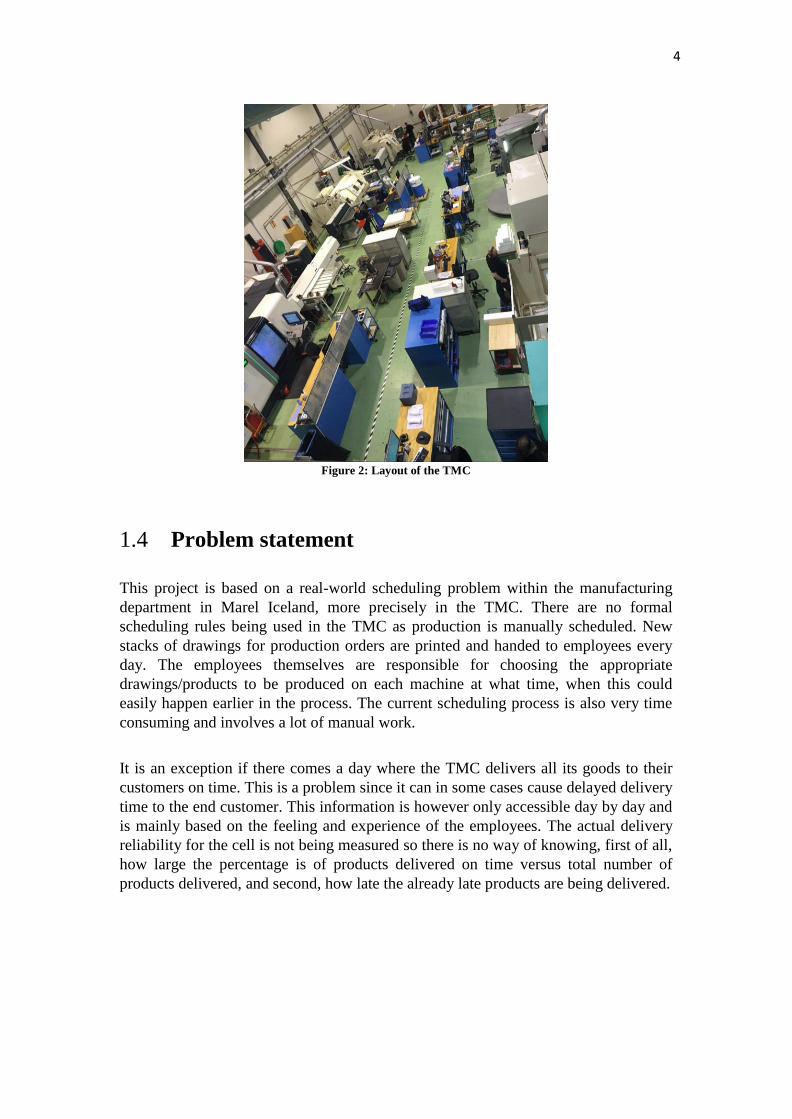
Figure 2: Layout of the TMC............................................................................................................ 4

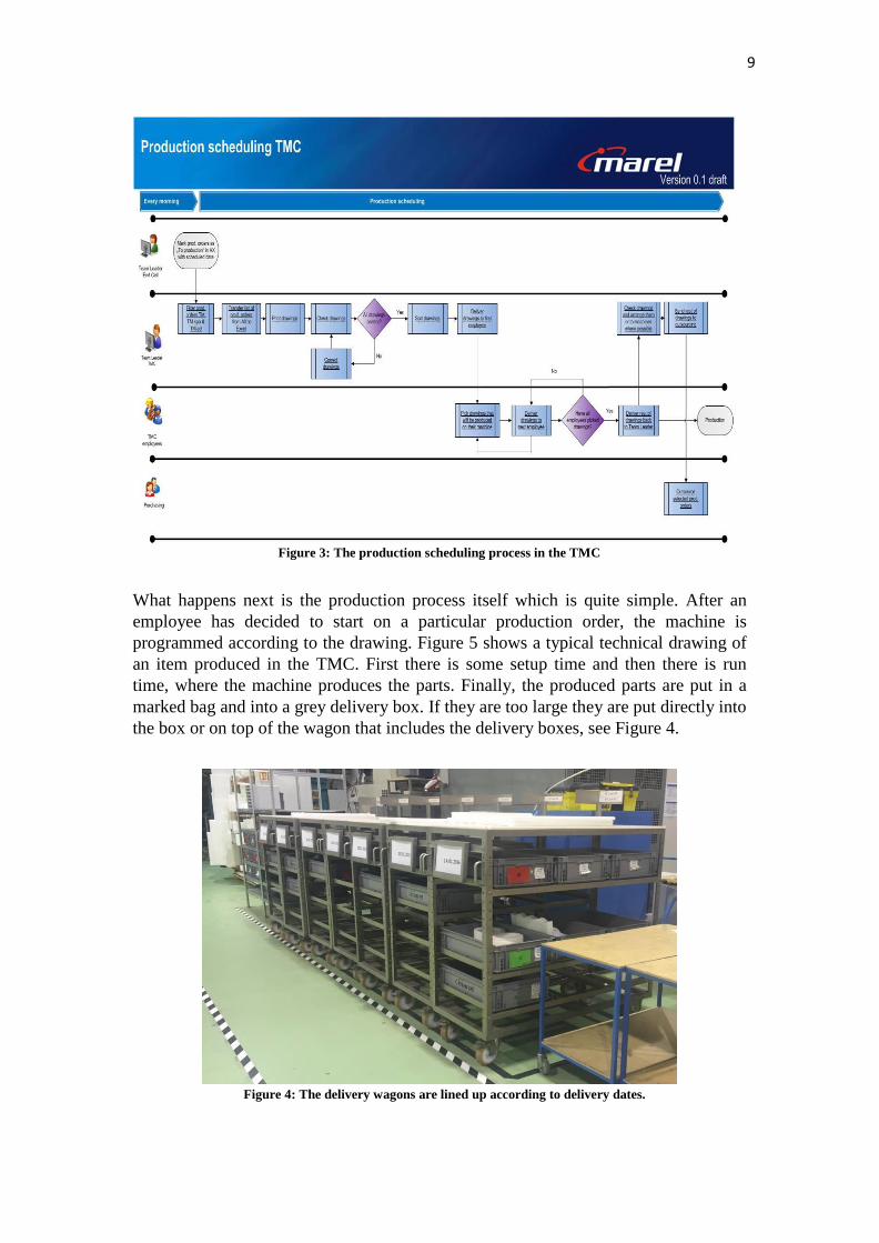
Figure 3: The production scheduling process in the TMC ............................................................... 9

Figure 4: The delivery wagons are lined up according to delivery dates. ........................................ 9

Figure 5: A typical drawing of a milled part produced in the TMC ............................................... 11

Figure 6: Delivery reliability for the first three months of 2016 .................................................... 15

Figure 7: Late deliveries Jan 2016 .................................................................................................. 16

Figure 8: Late deliveries Feb 2016 ................................................................................................. 16

Figure 9: Late deliveries Mar 2016 ................................................................................................ 16

Figure 10: A simple application of the TSP ................................................................................... 19

Figure 11: A screenshot of the Excel file ....................................................................................... 28

Figure 12: TMC production 2014 ................................................................................................... 31

Figure 13: Production Jan 2016 ...................................................................................................... 34

Figure 14: Production Feb 2016 ..................................................................................................... 35

Figure 15: Production Mar 2016 ..................................................................................................... 35

Figure 16: OLE - Availability for End Cells .................................................................................. 36

Figure 17: Available hours versus ordered hours for each machine in January 2016 .................... 39

Figure 18: Available hours versus ordered hours for each machine in February 2016 .................. 40

Figure 19: Available hours versus ordered hours for each machine in March 2016 ...................... 41

Figure 20: Available hours versus ordered hours for each machine in January 2016 with EDD ... 44

Figure 21: The delivery reliability sheet ......................................................................................... 53

Figure 22: Real production Jan 2016. JIT production orders are highlighted in green. ................. 54

Figure 23: Real production Feb 2016. JIT production orders are highlighted in green. ................. 55

Figure 24: Real production Mar 2016. JIT production orders are highlighted in green. ................ 56

List of tables

Table 1: Shift schedule for the TMC ................................................................................................ 8

Table 2: TMC's customer categories .............................................................................................. 28

Table 3: Work center identification ................................................................................................ 29

Table 4: Calculation of available hours .......................................................................................... 37

Table 5: Available hours left to spare each month ......................................................................... 42

Table 6: Results if the EDD rule with preemptions would have been applied ............................... 43

xviii

1

Chapter 1

Introduction

In today’s manufacturing competitive markets, companies need to be capable of

delivering products to their customer at the right time, at the right cost and in the right

quality. When manufacturing companies fail to schedule their production in an

optimal way, the risk of not being able to deliver their products, according to the right

standards, increases. Scheduling deals with the allocation of available resources to

tasks over a given time period [1]. In the manufacturing environment the resources are

usually machines and/or employees. It can be both challenging and time consuming to

create a good schedule as it is a decision making process with the goal of optimizing

one or more objectives, but a good and disciplined scheduling process can result in

better utilization of resources and therefore in higher delivery reliability to the end-

customer.

The thesis is the result of work done in the period of January to May 2016. During the

time of writing the thesis, the author was employed at Marel in Iceland.

1.1 Marel

In terms of total sales, Marel is amongst the ten largest companies in Iceland [2].

Marel is an innovative manufacturing company considered to be the leading global

provider of advanced equipment and systems for three different food processing

industries; poultry, meat and fish. Marel originated in Iceland in 1983 but since then it

has become the global phenomenon it is today, with over 4.500 employees working in

manufacturing, offices and subsidiaries in over 30 countries worldwide [3].

2

Marel’s primary goal is to advance food processing by delivering market-driven

innovation that helps their customers proactively adapt to continually changing

consumer habits and environmental challenges. The vision is of a world where quality

food is produced sustainably and affordably [3]. One of its core values is its

partnership with customers and the focus on creating added value. Therefore, Marel

does not only sell standard products but also customized products which can be

designed closely with the customers in order to fulfill their needs. Figure 1 shows an

example of a streamline for poultry processing, a product produced at Marel.

Figure 1: Streamline for poultry processing

Cellular manufacturing 1.2

Cellular manufacturing is a method from the lean manufacturing toolbox, focusing on

how manufacturing companies can organize their workshop floor. In cellular

manufacturing, production work stations and equipment are arranged in a sequence

that supports a smooth flow of materials and components through the production

process with minimal transport or delay. Cellular manufacturing is a method which

seeks to minimize the time it takes for a single product to flow through the entire

production process [4].

Marel is currently basing their manufacturing floor on cellular manufacturing and has

a total of 14 cells which all play a part in the production process. Marel has 6 support

cells: Turning and Milling Cell, Sheet Metal Cell, Glass Beading Cell, Electronic

Cell, Printed Circuit Boards cell and the Inventory Cell. The support cells provide

components to the end product cells in order for them to be able to assemble the final

product. There are two types of end product cells: SP cells which produce standard

products and Grader cells which produce customized products. There are four SP

cells, SP1- SP4 and four Grader cells, FL1-FL4. Furthermore, there is a Spareparts

Cell within SP1 and each cell has its own Team Leader.

3

The Turning and Milling Cell 1.3

The Turning and Milling Cell (from now on referred to as TMC), one of the support

cells within Marel Iceland, is the main focus of this project. The cell operates by the

Make-To-Order strategy, which means that production of goods only occurs after a

customer’s order is received [5]. Along with the customer’s order the cell receives a

requested delivery date from the customer.

The TMC produces around 1400 to roughly 2000 production orders every month,

where amount of items in each production order can vary from 1 to 300. However, the

average production order has only 6 items. The items produced are turned and milled

parts made mainly from steel and plastic, and production is carried out according to

drawings from designers that should include relevant and technical specifications.

The employees in the TMC are encouraged to arrange their production according to

the Just-In-Time (JIT) strategy, made popular by Toyota in Japan in the 1970s-80s.

Simply put, JIT is an inventory strategy companies use to increase their efficiency

and decrease waste by producing goods only when they are needed in the production

process and thereby reducing inventory costs [6].

The JIT strategy translates to the TMC and its employees in such way that production

should not occur too late but at the same time not too early. Therefore, unnecessary

batch production ahead of time is highly discouraged. Supporting that argument is the

fact that the flow of production orders into the cell are extremely fluctuating, both in

quantity and in product types as well as there are at least 300 new items introduced

each month, so item variability can be considered quite high. All of this results in the

fact that there is no effective forecast available for the TMC that could help with their

planning.

TMC has a production of high-mix/low-volume items which means that there can be a

lot of new things which have to be responded to during each day. A total number of

22 employees work in the cell, including the Team Leader. There are 4 lathes and 7

milling machines operating in the cell. Figure 2 shows the layout of the cell.

4

Figure 2: Layout of the TMC

Problem statement 1.4

This project is based on a real-world scheduling problem within the manufacturing

department in Marel Iceland, more precisely in the TMC. There are no formal

scheduling rules being used in the TMC as production is manually scheduled. New

stacks of drawings for production orders are printed and handed to employees every

day. The employees themselves are responsible for choosing the appropriate

drawings/products to be produced on each machine at what time, when this could

easily happen earlier in the process. The current scheduling process is also very time

consuming and involves a lot of manual work.

It is an exception if there comes a day where the TMC delivers all its goods to their

customers on time. This is a problem since it can in some cases cause delayed delivery

time to the end customer. This information is however only accessible day by day and

is mainly based on the feeling and experience of the employees. The actual delivery

reliability for the cell is not being measured so there is no way of knowing, first of all,

how large the percentage is of products delivered on time versus total number of

products delivered, and second, how late the already late products are being delivered.

5

The main problem in question is twofold. Firstly, we are looking at a scheduling

problem i.e. how production orders for multiple product types are organized onto

machines. Secondly, the employees of the cell are dealing with a lot of paperwork and

time which goes into printing, checking, organizing drawings etc. So on the one hand

there is the scheduling problem while on the other hand there is the lean

manufacturing problem where a lot of extra steps are being taken during the

scheduling process when they might not be necessary. During this project the main

focus will be on the scheduling problem, focusing on due-date related objectives.

The main objective of this project is to take this problem, analyze it in regards to

scheduling theory and from that analysis come up with a good and more automated

solution to the problem.

The research question being answered is the following:

By using the current resources in place, is it possible to improve the production

scheduling process by focusing on eliminating waste in the process flow in order to

minimize late deliveries on TMC’s products?

The goal for the TMC is therefore to deliver as many production orders as possible on,

or before, the requested delivery date. Or, to relate it to theory, to minimize the

tardiness.

Structure of the thesis 1.5

The structure of the thesis is as follows: Chapter 2 is a detailed analysis of the

problem. Chapter 3 discusses delivery reliability and Chapter 4 is a literature review

where the methods used to get closer to the solution are explained. Chapter 5

describes the dataset used in the project and the results and suggestions for

improvements are presented in Chapter 6. Conclusions are discussed in Chapter 7.

6

Contributions 1.6

The following contributions will be delivered through this project:

To Marel:

Process and data analysis

The current manual scheduling process in the TMC is analyzed and mapped up in a

flow chart. Ideas for improvements by focusing on eliminating waste in the process

flow are put forth, and a KPI introduced in order to encourage employee engagement

in reaching the company’s goal of improving delivery reliability.

Data for the first three months of the year 2016 was gathered and a comparison is

made between the real delivery reliability performance and the performance that could

have been achieved if scheduling rules would have been applied. By gathering new

data and displaying the results in a way that has never been done before in the Turning

and Milling Cell, understanding is increased and new light shed on underlying

problems prompting the Production Management in Marel Iceland to take action.

New scheduling methods introduced

Faults in the data registration are highlighted and new methods for scheduling the

production orders in TMC are introduced. Furthermore, suggestions for improving the

data registration in the cell are made in order to create a better foundation for applying

more advanced scheduling solutions.

To theory:

Actual scheduling problem connected to theory

Mathematically describing the real-life scheduling problem in a formal notation

provides an opportunity to compare the problem to other similar cases and relate it to

theory. In order to use theory in production scheduling, certain criteria needs to be

met, which is highlighted in the project.

7

Chapter 2

Detailed analysis of the problem

The current situation in the TMC was analyzed thoroughly. The author spent a few

days in the cell for observation purposes and information gathering, from both the

employees and the Team Leader. Both ways of working and the morale in the cell was

explored, in order to get a better feeling of how the production is planned and be able

to identify more opportunities for improvements.

It became clear that the cell has a strong culture and that the employees believe that

their ways of working are optimal for the company. There is little or no overview of

the status of production. For an outsider, e.g. a customer who is looking for

information about an item that is already late, there is no way of seeing when or on

which machine it will be produced. The person would have to walk up to every

machine and look through multiple stacks of drawings in order to find the item, and

basically ask the employee when the item will be produced.

This chapter describes the production cell in more detail as well as giving a more

thorough analysis of the scheduling problem.

8

The customers for the TMC are currently being segmented into three categories,

characterized by delivery time, based on how high they rank in priority decided by the

TMC and Production Management. The customers are Product Development, the

Spareparts cell and the End product cells.

The operation time for each of the 11 machines in the production cell is the same; five

days a week in two shifts, a day shift and a night shift. Table 1 shows exact work

hours and breaks for each day.

Table 1: Shift schedule for the TMC

TMC Days Work hours Break Lunch

Day shift Mon – Thu 06:00 - 15:00 09:00-09:10 12:00-12:30

Fri 06:00-12:00 09:00-09:10

Night shift Mon – Thu 15:00 - 00:00 21:00-21:10 17:30-18:00

Fri 12:00-18:00 15:00-15:10

The scheduling process has been examined and mapped up by the author of this

thesis. What triggers the process is when the Team Leader in the TMC filters out

production numbers marked with the status “To Production” in Marel’s enterprise

resource planning (ERP) system, Dynamics AX. The system is a production system

that holds all information regarding production orders and planning.

The Team Leader filters out production orders with delivery dates up to two weeks

into the future. The process is executed every morning when the Team Leader shows

up to work and can take up to a few hours, depending on the amount of interruptions.

Without any interruptions it is assumed to take around two hours to get the task done

each morning.

A flowchart was made in order to help the author to both visualize the steps in the

process and analyze where the biggest problems lie. The flowchart was made based on

information gathered from discussions with both the Team Leader of the cell and its

employees, during the days spent in the cell for observation purposes.

Figure 3 displays the flow chart of the current production scheduling process for the

TMC. The process looks overly complicated where there are multiple steps taken

while manually scheduling the production. The purpose of this project is again, to

come up with a solution to simplify this process.

9

Figure 3: The production scheduling process in the TMC

What happens next is the production process itself which is quite simple. After an

employee has decided to start on a particular production order, the machine is

programmed according to the drawing. Figure 5 shows a typical technical drawing of

an item produced in the TMC. First there is some setup time and then there is run

time, where the machine produces the parts. Finally, the produced parts are put in a

marked bag and into a grey delivery box. If they are too large they are put directly into

the box or on top of the wagon that includes the delivery boxes, see Figure 4.

Figure 4: The delivery wagons are lined up according to delivery dates.

10

2.1 Outsourcing and recent changes within the TMC

In some cases a production order comes through the production system in the TMC,

where the cell does not necessarily produce the part but outsources it to other

companies and contractors in Iceland. The reasons behind the choice of which

products are outsourced, are not clear.

Today, a significant part of the outsourced products are chosen in order to minimize

the load in the cell. In those cases, the products are usually the more complicated

products, e.g. products that have to go through both a turning and milling process.

Some of Marel’s contractors have access to more advanced machines and can

therefore produce those products more quickly. The main reason behind outsourcing

those products is to improve the flow in the TMC.

On the other hand, there has been more focus recently towards outsourcing high-

runner items (and getting fixed prices for them from contractors), to be able to free up

capacity for the more complicated items and by doing that, strengthening TMCs

position to be able to provide better service to Product Development. This vision, to

outsource more standard items which are sold more regularly, in order to free up

capacity for customized items, is considered appropriate in the TMC since the

production in the cell is categorized as high-mix/low-volume. The cell should be

highly responsive and flexible, which might go against economies of scale, again

underlining the focus on outsourcing high-runner items.

However, the amount of outsourced production orders without fixed prices so far this

year are estimated to be around 150-600 production orders (or 9000-11.500 items) per

month. That amounts to around 15-18% of the production orders that originally come

into the production system from the TMC’s customers per month. These numbers do

not include the outsourced items that Marel has in contract (i.e. with fixed prices). So,

the items that are usually outsourced are done so on short notice and can therefore

become more expensive. The cost of outsourcing these production orders have, for the

first three months of this year, accumulated to 140.000€.

The make or buy decision, on which types of products should be outsourced and

which should not, is not the main point in this research. However, it is something that

needs to be addressed by Production Management as it would give the TMC much

better direction on what jobs to keep in-house and which jobs to outsource.

11

In January 2016 the TMC went through changes which underline the need for a

refined production scheduling solution. Before the changes were made, there were

two Team Leaders working in the cell who took turns in managing the day shift

versus the nightshift. Multiple reasons led to one Team Leader being transferred to a

new position, an operational purchaser for the TMC. One of the reasons was the

increase in outsourcing which called for resources with a lot of product knowledge

performing that task for the cell.

Therefore, one of the Team Leaders was selected for the job which means that today

there is only one Team Leader operating in the cell and he works during the day shift.

The cell operates itself during the night shift, i.e. the employees work on their tasks

during the night shift with no Team Leader. There is no particular production

scheduling done for the night shift and none for the day shift either for that matter, as

each machine gets its stack of drawings of items that have been released for

production from Dynamics AX by the Team Leader.

Figure 5: A typical drawing of a milled part produced in the TMC

13

Chapter 3

Delivery reliability

The problem concerning on-time deliveries from the TMC to its customers was

justified. There was no way of knowing the real delivery reliability since it was only a

common understanding within the company that there were usually shortages in

production orders from the TMC. It can also be related to the lack of overview of the

production status, not only to customers, but also to both to the Team Leader and the

employees in the cell. Therefore, the objective was getting clear key performance

indicators (KPIs) for the current situation and thus make it easier to see how much

potential progress this research could lead to and to have a real measurable progress

afterwards.

This chapter will explain why and how the current delivery reliability was found.

3.1 Delivery reliability as a KPI

A KPI is a business metric used to evaluate factors that are crucial to the success of an

organization [7]. In other words, KPIs are a way of measuring how well an individual,

a company, a business unit or even a production cell is performing. Bernard Marr, the

best-selling author and enterprise performance expert, discusses in his article “What

the heck is a KPI?” how the potential value of KPIs remains in the hands of those that

use them [8]. Marr establishes the importance of choosing the right KPI to ensure

employee engagement and favorable results. The right KPI needs to be aligned with

the company objectives; hence the choice of delivery reliability as a KPI in this

project as the objective is to improve on-time deliveries to customers.

14

Delivery reliability is a key strategic attribute in supply chain management. It can be

used as a KPI when measuring the success and quality of manufacturing companies.

Delivery reliability can have a great impact on the customers’ choice when he decides

who he would like to do business with. The customers want to make sure they get the

right product, for the right price delivered on the right time; the higher the delivery

reliability, the better. In calculating delivery reliability, the ratio of the number of

deliveries made without any error (regarding time, place, price, quantity and/or

quality) to the total number of deliveries in a specified period is found [9].

The Production Management in Marel has focused on measuring delivery reliability

as a KPI when measuring deliveries from their End cells to customers. However, there

is no reason why delivery reliability cannot also be used as a KPI to measure

performance on the workshop floor from the support cells to their customers. The

main focus is on measuring delivery dates, i.e. time, while price, quantity and quality

are always assumed to be correct.

Like mentioned earlier, the delivery reliability needed to be measured in order to

explore the current situation in the cell. An Excel sheet was designed based on the

query used in order to access the data in this research. The delivery reliability was

measured by the amount of production orders, not quantities, delivered on time versus

the total number of production orders processed in the TMC. The production manager

for TMC can now access and use the sheet in order to continue monitoring the

delivery reliability in the cell and regularly inform both the Team Leader and

employees in the cell of their performance.

The delivery reliability sheet can be found in Appendix A and the results for the TMC

for the first three months in the year 2016 are shown in a graph in Figure 6.

15

Figure 6: Delivery reliability for the first three months of 2016

When looking at Figure 6, the delivery reliability is very stable between months or

87.8% on average. The target of 95% delivery reliability is decided by Production

Management in Marel.

87.8% delivery reliability supports the information put forth in the problem statement

in Chapter 1.4, where the feeling from employees was that there was rarely a day

when TMC delivered all their products on time. Taking January as an example, a total

of 1430 production orders was delivered. If 87.8% of them were delivered on time

that gives a total of 175 late orders. With 20 work days in January that gives a result

of 8.75 late deliveries on average per day.

February delivered similar results or 11.10 late deliveries on average per day with a

total number of 1796 production orders. March had 10.45 late deliveries per day with

a total number of 2098 production orders. Note that these numbers show delivery

reliability for production orders that end up actually being produced in the TMC,

hence excluding all outsourced items.

The delivery reliability is calculated on a monthly basis, but in practice, in order to

encourage employee engagement, it would be better to measure down to weeks. That

generates both more detailed information and more frequent updates to the employees,

making it easier for them to be aware of their performance.

87,7% 87,6% 88,0%

75,0%

80,0%

85,0%

90,0%

95,0%

100,0%

Delivery reliability - TMC Monthly 2016

16

Further analysis of late deliveries was done in order to see how late they were actually

being delivered. In all three cases, over 68% of late deliveries were being delivered

within 5 days too late, as shown in Figures 7-9.

Figure 7: Late deliveries Jan 2016

Figure 8: Late deliveries Feb 2016

Figure 9: Late deliveries Mar 2016

65 prod. 37%

86 prod. 50%

19 prod. 11%

4 prod. 2%

Late deliveries - Jan 2016

1 day 2-5 days 6-10 days >10 days

81 prod. 36%

105 prod. 47%

30 prod. 14%

6 prod. 3%

Late deliveries - Feb 2016


102 prod. 41%

69 prod. 27%

53 prod. 21%

27 prod. 11%

Late deliveries - Mar 2016


17

Chapter 4

Methods

This chapter will explain in further detail how the problem was approached, and the

selection of tools and methods used to get closer to the solution is explained.

4.1 Scheduling

Production scheduling is often identified with Frederick Taylor, Henry L. Gantt and

Selmer M. Johnson. In 1911, Frederick Taylor defined the key planning functions and

created a planning office in his monograph, The Principles of Scientific Management

[10]. How he separated planning from execution justified the use of formal scheduling

methods, which became critical as manufacturing companies where growing fast in

complexity during this time [11]. His work was supported by Gantt, who provided

useful charts to improve scheduling decision making. Later on, Johnson, an American

mathematician, wrote a highly influential paper on the mathematical analysis of

production scheduling problems [11]. All in all, those three individuals took their own

approach on how to improve production scheduling. In short, Taylor changed the

organization, Gantt created tools to improve the decision-making process, and

Johnson solved optimization problems [11].

The most common scheduling problems, and the most manageable ones, involve

single or parallel machines [1]. More complicated problems are shop environments

which can be divided into three categories: open shop, flow shop and a job shop. As

[1] states, an open shop has no restrictions with regards to the routing of each job

trough the machine environment, so the scheduler is allowed to determine the route

for each job, and different jobs may have different routes in the production process.

18

A flow shop is where each job has to go through the same route through different

machines. A flexible flow shop has a number of stages and at every stage there are a

number of machines. In a job shop environment each job has its own route with n jobs

and m machines. So the main difference between a flow shop and job shop is that in a

flow shop, all products follow the same route through the production process but in a

job shop each product has its own route.

The problem considered in this research is classified as a job shop environment. As

mentioned before, the job shop problem is NP-hard [1]. The TMC resembles a job

shop production environment where each job has its own route. As stated in [1], a job

shop is a scheduling problem with n jobs and m machines. The job shop problem is

NP-hard and therefore difficult to solve to optimality [1]. A distinction is made

between job shops where each job visits any machine at most once and job shops

where a job may visit a machine more than once. In this case we are working with the

first example; however the complexity of this problem increases since a job may need

to visit two different machines in its production process, i.e. when a product needs to

go through both turning and milling.

The famous travelling salesman problem (TSP) has been proven to be NP-hard, and

the job shop problem is more difficult since the TSP can be formulated as a special

case of a job shop problem with m=1 (the salesman is the machine and the cities are

the jobs). Therefore, the job shop problem is also NP-hard.

A basic description of the TSP is that a salesman tries to find the shortest route that

passes through each of a set of points (cities) once and only once [12]. Figure 10

displays a simple application of the TSP. The Travelling Salesman Problem is a

mathematical problem that has been studied extensively all around the world for many

years. In Iceland back in 2005, Jensson, Kristinsson and Gunnarsdottir published an

article where they explained how they used two different methods to formulate this

famous problem, a genetic algorithm (GA) and an integer programming approach

[13].

In 1953, job shop problems were examined by S.M. Johnson. He introduced a

heuristic algorithm that can be used to solve the case of a 2 machine n job problem

where all jobs are to go through both machines and be processed in the same order

(also referred to as Johnson’s rule) [14]. There must also be no job priorities and the

time for each job has to be a constant.

19

Figure 10: A simple application of the TSP

Manual scheduling 4.2

As mentioned earlier, the TMC currently schedules its production manually based on

the production orders received through the production system. The Team Leader and

employees in the cell have a lot of experience and knowledge in their field so they are

capable of manually scheduling and delivering an acceptable performance.

In an Optisol article from 2013, Prasad Velaga talks about manual scheduling in

regards to job shop production [15]. Velaga states that a job shop production is in fact

manageable with manual scheduling but it can lead to increased work-in-progress

(WIP), longer lead times, poor on-time delivery and frequent firefighting. Manual

scheduling amounts to push scheduling, which is usually discouraged by lean

manufacturing experts [15]. Manual scheduling is further explained by this short

excerpt from the article:

“While struggling to meet the due dates, they do extensive real-time scheduling, that

is, firefighting without knowing the ripple effect of their real-time decisions on

production plan.”

This description fits well to the current scheduling arrangement within the TMC

today. The article also states that job shops cannot easily improve their performance

until the need for firefighting is minimized [15]. Furthermore, it describes how

inefficient manual scheduling is for complex job shops with high-mix/low-volume

production that need to be able to handle numerous diverse orders at any time, like in

the case of TMC.

Based on the views in this article, should scheduling methods be applied to the TMC,

it will result in increased delivery reliability, throughput and resource utilization in the

cell.

20

The Earliest Due Date (EDD) rule 4.3

The Earliest Due Date (EDD) rule is one of the simplest rules in scheduling theory.

The EDD rule gives the job with the earliest due date, based on assigned due dates,

the highest priority. A theorem stated in [1] explaines:

“The EDD rule minimizes expected maximum lateness for arbitrarily distributed

processing times and deterministic due dates in the class of nonpreemptive static list

policies, the class of nonpreemptive dynamic policies, and the class of preemptive

dynamic policies.”

Preemptions imply that it is not necessary to keep a job on a machine until

completion. In other words, when preemptions are allowed, the processing of a job

may be interrupted at any time and another job is allowed to be put on the machine.

The amount of processing a preempted job has already received is not lost and the job

can be resumed at any time [1].

To elaborate, if the EDD rule with preemptions would be applied in the TMC, it

would allow stopping the processing of a particular job one day and resuming it the

next day, without upsetting the flow of production.

Other scheduling rules worth mentioning, but will not be explained in detail, are the

first-come, first-served (FCFS) rule where the job arriving at the workstation first gets

the highest priority, the Shortest Processing Time (SPT) rule, the Critical Ratio (CR)

and Slack per Remaining Operations (S/RO) [16].

The EDD rule is considered most likely to be helpful to this project as it focuses on

due-date related objectives.

21

Mathematical description of the problem 4.4

Traditionally, when describing a scheduling problem it is put forth as a formal

notation (α|β|γ) consisting of three fields, where α describes the machine environment,

β describes the constraints and γ describes the objective which is to be minimized [1].

The use of this formal notation for theoretic scheduling problems was first introduced

in 1979 by Ronald Graham, Eugene Lawler, Jan Karel Lenstra and Alexander

Rinnooy Kan [17].

The scheduling problem in this case study is put forth as:

J11|pij, rj, dj |ΣTj

J11 denotes the machine environment which is a job shop consisting of 11 machines.

The constraints are pij, rj and dj and the objective function that is to be minimized is

ΣTj which represents the sum of tardiness of jobs j. The notation is explained further

in the following segment.

Machine environment, α

The machine environment in question is considered a job shop with 11 machines,

denoted as J11. A job shop is where the route of every job is fixed but not all jobs

follow the same route. Like stated in [18], a typical job shop is a “high-mix, low-

volume production unit that processes simultaneously several diverse, low-quantity

jobs using shared resources.”

In general, a job shop is a production unit where:

o order quantities are usually small

o process requirements vary with customer order

o processing starts for an order only after receiving the order from customer

By this description, most custom manufacturing units in the real world qualify as job

shops, and the subject in this case study is no exception.

22

Constraints, β

Three constraints are defined in the notation. Since the scheduling problem has a due

date related objective, there needs to be at least one date related constraint. Therefore,

we have the release date, rj. According to [1] the due date, dj is sometimes not

specified in the description as it is clear from the objective that we are working with

due dates, but in this case dj is a part of a notation as well.

The constraint pij denotes the processing time of job j on machine i. The subscript i is

usually omitted if the processing time of job j does not depend on the machine or

when job j is only to be processed on one give machine [1]. This constraint is

interesting since the job shop concerned involves some cases where a job is only to be

processed on one given machine and then other cases where a job can be processed on

more than one machine. The right thing to do is to include the i and make the

constraint pij, since in reality the time spent on any given job varies between

machines. However, the next chapter will highlight how, with the dataset given, the

constraint would need to be pj in practice for the problem in this case.

All setup times are assumed to be sequence independent, where they will simply be

added to the processing times. Therefore, there is no constraint regarding the setup

time in this notation.

Along with the before mentioned constraints, there are also constraints that are valid

for all job shops. Firstly, each machine can only process one job at a time. Secondly,

each job can only be processed by one machine at any time. And thirdly, since

preemptions are not allowed, once a machine has started processing a job, it will

continue running on that job until it is finished. Lastly, the number of jobs n and

number of machines m are finite numbers.

The objective function, γ

Generally, there are three basic due-date-related penalty functions; lateness (L),

tardiness (T) and the unit penalty (U) [1]. When choosing the most appropriate

objective these three functions were examined.

23

Lateness of job j is defined as

Lj = Cj – dj

Tardiness of job j is defined as

Tj = max(Cj – dj;0)

Unit penalty of job j is defined as

Uj = {1 if Cj > dj

0 otherwise

Cj is the completion time of order j and dj is the due date (the requested delivery date

made by TMC’s customers) for order j. In this case, the orders are being scheduled for

multiple product types with a due date related objective.

By choosing ΣLj as the objective to be minimized, it would encourage the employees

in the TMC to produce orders as early as possible. That does not support the JIT

strategy which should be being pursued in the cell, and is therefore not a good fit for

the objective.

Choosing the numerical value of ΣLj, Σ|Lj|, as the objective would however come

closer to the desired result. The advantage gained that way, is that production is

encouraged to happen on the scheduled due date, or just-in-time, since there would

never be a negative value. In that case however there wouldn’t be any distinction

between a production order being produced a day early or a day too late. This could

be the most feasible objective in some cases. However, in this case it is not always

possible to produce all production orders on the scheduled due date, due to

fluctuations in demand. This would therefore give misleading results.

The unit penalty or total number of late orders, ΣUj, could also be chosen as the

objective. However, that does not give any distinction between late production orders

being delivered a day too late or e.g. 14 days late, when it is obvious which is more

feasible.

By choosing tardiness over lateness, all productions that occur before the scheduled

due date get the same value, 0, as if they were produced on that exact date instead of

the negative value they would get if we were minimizing lateness. Tardiness is

positive when a product is delivered late and zero when a product is delivered on or

before the due date.

Therefore, minimizing tardiness, ΣTj, was considered to be the best fit to the criteria.

24

Recent work 4.5

Multiple research studies have been done in collaboration with manufacturing

companies in Iceland, Marel included.

In 2010, H. Ludviksson did a research that involved identifying reasons for high

inventory costs for one of the support cells, Printed Circuit Boards Cell. Ludviksson

made recommendations in his work based on lean methodology that could reduce

inventory cost in the future [18].

More recently, in 2015, R. Valgeirsdottir studied the production process in the End

product cells FL1-4 which produce customized products [19]. Valgeirsdottir focused

on discovering opportunities where the lead time could be shortened by minimizing

the slack in the production system, and making suggestions to Production

Management at Marel. It was specifically pointed out how the overview of the

production system could be improved. That is familiar to the situation in the TMC,

where even the Team Leader does not have any accessible overview of the status of

production in his production cell.

In 2012, P.Winrow analyzed the delivery reliability for Make-To-Order productions at

a company called Plastprent. By using a supply chain operation reference model

Winrow analyzed the processes that were affecting the delivery reliability and from

that delivered improvement suggestions to the company [21].

R. Gudmundsdottir studied a scheduling problem for a pharmaceutical company in

2012. The company’s workshop was categorized as a flow shop with organized batch

production. Gudmundsdottir was able to automate the scheduling process by

introducing an optimization model that arranged orders in a campaign plan, where a

short term schedule based on a long term campaign plan was made [20]. In this case,

there were product families to work with and a sales forecast at hand, which certainly

can help a lot when applying scheduling methods.

Gudmundsdottir’s research was inspired by a study by H. Stefansson from 2006

where a dataset from the same pharmaceutical company was used and a multi-scale

modelling approach with three hierarchical levels of decisions was introduced [22].

G.H. Axelsdottir also studied the same problem [23, 24], with the focus on short term

planning and scheduling jobs to preplanned campaigns using a mixed integer model.

It was shown that it was possible to automate the scheduling process in question.

25

Chapter 5

Dataset

The data used in this research was acquired through the company‘s enterprise resource

planning (ERP) system, Dynamics AX. The system is a production system that holds

all information regarding production orders and planning. To acquire the necessary

data from the system a query was made in order to transfer information over to a

Microsoft Excel file.

The file appears as a one sheet list including all production orders for the production

cell, whether the order has already been produced or remains to be produced. The

sheet list contains one line for each production order, and multiple columns describing

that production order i.e. a production id number, production pool, status of

production, work center, item id number, process time, quantity, delivery date and

physical date. Figure 11 shows the Excel file that was created through the query to

Dynamics AX.

26

The sheet makes it possible to filter out any column when necessary and in the

following segment every column will be explained in detail.

PRODID: Production identification number or a production order number. Each

production order gets its own number but the number of items produced in each

production order can vary from 1 item to over 200 items.

PRODPOOL: Production pool. Implies which customer the production order

belongs to. In this research the focus will be on scheduling the three main customers

TM, TM-SPA or TM-PD. To note, when an outsourcing decision is made for a

particular production order, the production pool changes into TM-OUT in Dynamics

AX, and therefore the relevant line disappears from the list in the file.

The customer categories and their pre-promised delivery time are displayed in Table

2. To explain further, Product Development can create a production order in

Dynamics AX and expect a delivery in 5 days’ time whereas a Team Leader from an

end cell has to assume at least 14 days for his item to arrive.

STATUS: The status of the production order. There are seven different statuses

each production order will have at some point. The order is created, estimated,

scheduled, released, started, reported as finished and ended. What happens in each

status is described in further detail here below:

Created: The production order is created. At this stage there is no requirement

in the system and the production order remains invisible to the TMC.

Estimated: Production order is estimated by the Team Leader in the End

Cells/Spareparts Cell or Product Development. This estimates work hours and

cost for the main production, but the order still remains invisible to the TMC.

Scheduled: Production order is scheduled by the Team Leader in the End

Cells/Spareparts Cell or Product Development where they put in the requested

delivery date. Here the production order becomes visible to the Team Leader

in the TMC.

Released: The Team Leader in TMC has “released” the production order as

ready for production i.e. he has printed out the appropriate drawing and

delivered it to his employees. This happens between 1 or 14 days before the

delivery date.

Started: This means the production has started. An employee in TMC has

started producing the items according to the drawing.

27

Reported as finished: Production has been completed with all produced items

for the relevant production order having been placed in the appropriate

delivery box. The delivery box is taken to the relevant customer on the

scheduled delivery date.

Ended: The production order has been charged in the system by the Production

Manager of the TMC.

WRKCTRID: Work center identification. This column shows which machine

each production order should be produced on. Sometimes there are products that can

be produced on more than one machine. However, this field only shows one

suggestion. In the case where an item has to go through two different machines

(turned and milled part) there will be two lines with the same PRODID number. Table

3 shows the WRKCRTID for each of the 11 machines available, machine type and

name as well as which material is used for production on each machine.

PROCESSTIME: Shows the runtime in hours, per item.

DLVDATE: Shows the scheduled delivery date, which comes directly from the

customer when a new production order is placed into Dynamics AX with the status

“Scheduled”. The requested delivery date by the customers is used as the due date.

DATEPHYSICAL: Shows the exact date when the production was changed from

“Started” to “Reported as finished”. This column makes it possible to gather reliable

data back in time, and also to see both how early and how late production orders are

being produced.

QTYCALC: Shows the amount of items which are included in the production order.

This is the number of pieces that should be produced and delivered to the customer.

ITEMID: This is the item identification number which is displayed on the

drawing.

28

Figure 11: A screenshot of the Excel file

Table 2: TMC's customer categories

PRODPOOL Customer Promised delivery time

TM-PD Product Development 5 days

TM-SPA Spareparts cell 10 days

TM End cells 14 days

29

Table 3: Work center identification

WRKCRTID Machine name and material Type

oku_10 Okuma 10 – plastic/steel Turning

oku_15 Okuma 15 – plastic/steel Turning

gild_800 Gildemeister 800 - plastic/steel Turning

gild_320 Gildemeister 320 - plastic/steel Turning

htm Htm – plastic Milling

reichen Reichenbacher 1 – plastic Milling

reichen Reichenbacher 2 – plastic Milling

dmc_63 DMC63 – plastic Milling

oku_45 Okuma 45 – plastic/steel Milling

oku_55 Okuma 55 – plastic/steel Milling

dmu_100 DMU 100 – plastic/steel Milling

30

5.1 Data analysis

Since the Excel file gathers data from Dynamics AX, it is important for the query in

Excel to be refreshed every time before it is used in reality. That ensures that the data

is always up to date, and contains, for example, all recently added production orders

as well as all information about all production orders that have been outsourced and

therefore get erased from the production lines (since it has been put as „TM-OUT“ in

the PRODPOOLID column).

Thus, the data sheet does not contain any fixed number of future production orders

that need to be scheduled, since it is a “constantly alive” production system where

customers can add orders, postpone orders etc. All that the sheet needs, to keep up

with the production system, is that it is refreshed.

Since the column DATEPHYSICAL makes it possible to gather reliable data back in

time, it was decided to use data from the first three months of the year 2016 in this

analysis to compare the real performance of the TMC versus what could have been

done if scheduling rules would have been applied. By choosing to do so the query did

not need to be refreshed every time, because there are no changes being made to the

production system back in time (expect for maybe the status going from reported as

finished to ended, but that does not have any influence on delivery time).

To note, the fact that each production order is already marked with an appropriate

machine (WRKCTRID) when the production order enters the production system, it

limits the way scheduling methods could be applied on the data. In reality, most of the

products can be produced on more than one machine, with different run times

depending on the machine. However, the data does not give the option of choosing

available machines, which would be necessary in order to automatically and optimally

arrange production orders onto different machines.

Furthermore, since there is no information on the setup time available through the

data, assumptions for all the multiple product types has to be made, which in reality is

not recommendable since it can never give detailed enough information in order to

optimally schedule the production orders. Adding to that, the setup time in reality can

be diverse between machines so again, since there is only one machine behind each

production order limits the problem even more.

There are no preventive maintenance times registered in the data as in reality there is

no preventive maintenance performed in the TMC. When a machine breakdown

occurs, the machine is fixed and production is simply down during the time it takes to

fix it. When that happens, that time is nowhere registered in the production system so

all actual maintenance times appear invisible through the data.

31

It has been established that the dataset possesses multiple disadvantages when trying

to connect it to scheduling theory. With the current data available, simpler scheduling

rules and strategies have to be relied on in order to improve the scheduling process in

the TMC.

High-mix/low volume production 5.2

Figure 12: TMC production 2014

As mentioned in Chapter 1.3, TMC has a production of high-mix/low-volume items.

Figure 12 shows how many times each item number is produced in the TMC over the

course of 1 year.

When gathering information on the variance of produced items, the data received

showed that the total number of different items produced in the production cell was

3672 during the year 2014. According to Production Management in Marel, the

numbers are assumed to be at least similar if not higher for the year 2015, with the

same trend materializing in YTD 2016. This means that on average there are at least

300 different item numbers being produced each month.

Interestingly, 51.8% of items produced in 2014 belonged to only 1-4 production

orders, as new item numbers are frequently introduced by Product Development with

around 300-400 new item numbers filed into the production system per month. Item

variability is therefore considered to be very high and when comparing those numbers

32

to other similar manufacturing companies in Iceland in the industry, it can be assumed

that the TMC is in fact producing a range of high-mix/low-volume items.

When producing new items it is inevitable that the setup time is longer than for a

high-runner product. There has to be some programming performed and in some cases

employees from Product Development (one of the TMCs customers) work closely

with employees from the TMC while the product is still in the design phase. Again,

since the data given does not include any setup times, and some assumptions have to

be done for simplification reasons, this does not necessarily reflect the correct

information, especially when it comes to production orders for TM-PD. In this

research however, the overall setup time is assumed to be 25% versus 75% runtime

for each product.

In reality, longer setup times actually encourage employees to produce ahead of time

(batch production) so they don’t need to setup again for the same or similar product

day after day. But according to the data, fewer than 20% of all item-numbers

produced in the cell are produced in more than 20 pieces over the course of a whole

year. That fact, along with the JIT strategy which is being pursued, is another reason

that underlines once again why batch production is strongly discouraged.

33

Chapter 6

Results

The scheduling problem concerned in this thesis was approached in such way that the

data for the first three months of 2016, January-March, was used. The data was

analyzed using Microsoft Excel.

This chapter delivers the main results and the comparison between the real

performance and the performance that could have been achieved if scheduling rules

would have been applied.

6.1 Real production

Assuming the JIT strategy is being followed, the delivery reliability numbers raise the

question whether the machines are either not capable of handling the load of

production orders, leading to even more outsourcing, or that some organized batch

production would be something to consider in order to increase the numbers.

However, when exploring the data for each month further, it can be shown exactly

how many days before or after the scheduled delivery date production is being

performed. By doing so, it becomes obvious that the JIT strategy is not being

followed directly. Even though in most cases production orders are being produced on

the same day as its scheduled delivery date (which is considered to be on-time and

JIT), orders are also commonly produced up to two weeks ahead of time and in the

worst cases up to 49 days ahead. At the same time, the TMC manages to deliver late.

34

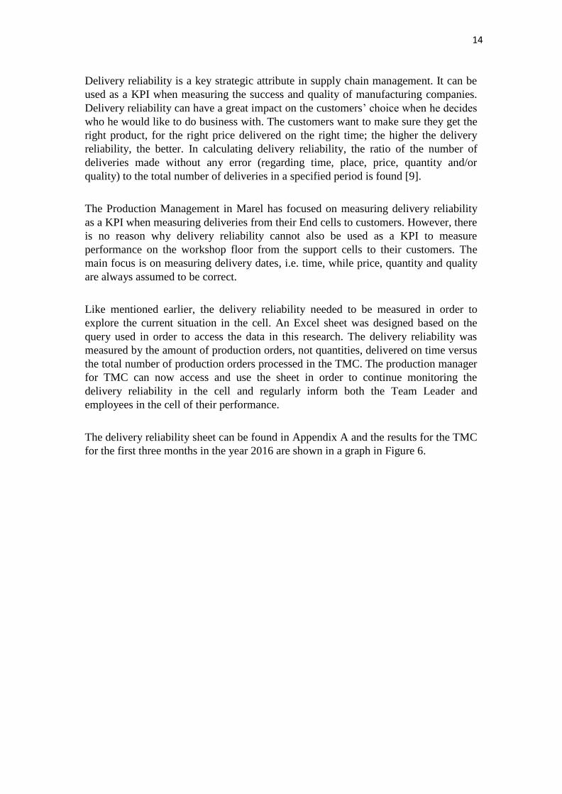
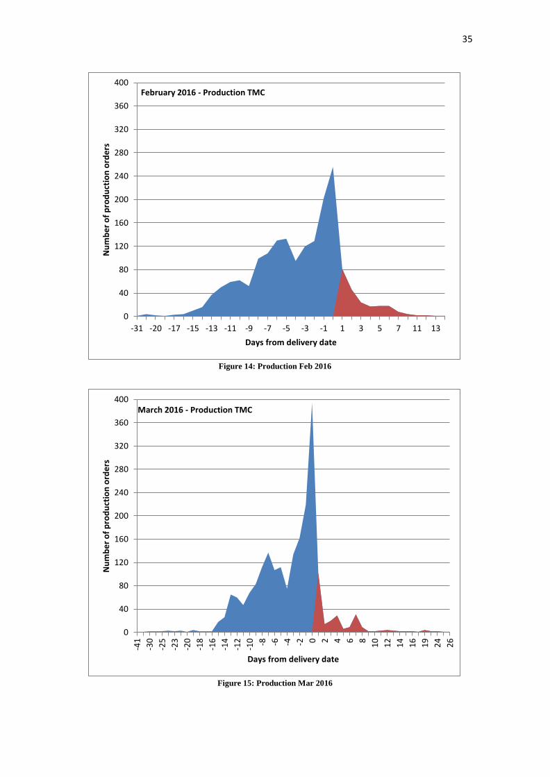
Figures 13-15 show the real production performance of the TMC for the first three

months of the year 2016 by manually scheduling with the objective to minimize the

tardiness. The employees should be keeping in mind the JIT strategy that is being

pursued in the company in order to minimize inventory costs, but like previously

mentioned, they do not appear to be following the strategy as strictly as one would

think.

The blue areas show the production orders that were delivered on or before the due

date and the red areas show late deliveries. The x-axis shows at what time the

production order was produced in regards to the scheduled delivery date. Furthermore,

if a production order was produced on the delivery date it gets the value 0 (which is

the case in most instances). If a production order was produced before the scheduled

delivery date it gets a negative value and likewise, it gets a positive value when

produced late. The y-axis shows how many production orders were delivered on each

date, on, before or after the scheduled delivery date.

Figure 15 shows the highest peak of just under 400 production orders produced on the

scheduled delivery date, but the peak can partly be explained by the fact that out of

the three months, March had the highest number of total production orders.

The detailed data that Figures 13-15 are based on is displayed in Appendix B.

Figure 13: Production Jan 2016

0

40

80

120

160

200

240

280

320

360

400

-49 -40 -33 -29 -27 -24 -22 -20 -17 -15 -13 -11 -9 -7 -5 -3 -1 1 3 5 7 9 17 32

Nu

mb

er

of

pro

du

ctio

n o

rde

rs

Days from delivery date

January 2016 - Production TMC

35

Figure 14: Production Feb 2016

Figure 15: Production Mar 2016

0

40

80

120

160

200

240

280

320

360

400

-31 -20 -17 -15 -13 -11 -9 -7 -5 -3 -1 1 3 5 7 11 13

Nu

mb

er

of

pro

du

ctio

n o

rde

rs


February 2016 - Production TMC

0

40

80

120

160

200

240

280

320

360

400

-41

-30

-25

-23

-20

-18

-16

-14

-12

-10 -8 -6 -4 -2 0 2 4 6 8

10

12

14

16

19

24

26

Nu

mb

er

of

pro

du

ctio

n o

rde

rs


March 2016 - Production TMC

36

Calculation of available hours 6.2

With the purpose of finding out how much improvement could have been

accomplished if scheduling according to the JIT strategy had been applied at the

beginning of the month, it was decided to explore first how many available hours each

machine had per month. That way it would be possible to organize the production

according to the capacity of each machine.

Four days a week, the shifts have a total of 16.5 available hours when breaks have

been deducted (11.25 hours on Fridays). Because of faults in the data, the setup time

needs to be estimated. As previously mentioned in Chapter 5.2, it is assumed to be

25% against the run time of 75%. The setup time varies between products, and even

machines, but this is an overall assumption based on information from both

Production Management and employees in the cell. Normally it is assumed to be from

10-30% depending on the product so choosing 25% for the setup time overall is a

rough assumption.

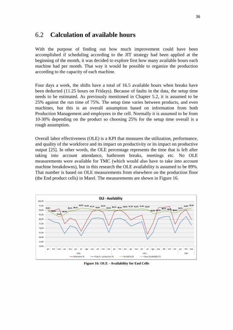
Overall labor effectiveness (OLE) is a KPI that measures the utilization, performance,

and quality of the workforce and its impact on productivity or its impact on productive

output [25]. In other words, the OLE percentage represents the time that is left after

taking into account attendance, bathroom breaks, meetings etc. No OLE

measurements were available for TMC (which would also have to take into account

machine breakdowns), but in this research the OLE availability is assumed to be 89%.

That number is based on OLE measurements from elsewhere on the production floor

(the End product cells) in Marel. The measurements are shown in Figure 16.

Figure 16: OLE - Availability for End Cells

37

To conclude, the calculation of available hours is given under the following

assumptions:

All machines are available at any moment and there is an employee working

on each machine at all times.

Runtime is 75% of available hours (versus 25% setup time)

Availability is 89%

Table 4: Calculation of available hours

Timetable

From To Tot. hrs Breaks Avl. hrs Runtime/Avl. hrs. /Calc. OLE

Mon 06:00 23:59 17:59 01:30 16:29 12:22 11:00

Tue 06:00 23:59 17:59 01:30 16:29 12:21 11:00

Wed 06:00 23:59 17:59 01:30 16:29 12:21 11:00

Thu 06:00 23:59 17:59 01:30 16:29 12:21 11:00

Fri 06:00 17:59 11:59 00:45 11:14 08:25 07:29

Table 4 displays how the availability of 11 hours per day (7.5 hours on Fridays) was

calculated.

After taking the assumptions into account what is left is that each machine has 11

hours available for runtime out of the 18 hours that employees are working in the cell

(7.5 hours on Fridays). That leads to the fact that during 61.1% of the total available

time each day, the machines could possibly be running.

It is debatable whether that number is sufficient, and perhaps it would be more

realistic to calculate that number down to each machine as some might have more

setup time and others less, but in this research, for simplification reasons, all machines

are assumed to have the same amount of available run time each day.

Again, because of faults in the dataset, it is impossible to realize which production

orders can be produced on which machines, other than the one stated in the “work

center identification” column in the dataset. That fact limits the ability to move

production orders automatically between machines like can be done in reality.

38

Applying the JIT strategy 6.3

With available run time per day for each machine being 11 hours (7.5 hours on

Fridays), gives the machines 206 available hours each month consisting of 20

workdays (23 in March). Considering the nature of the real production displayed in

Chapter 6.1, what was explored was if the JIT strategy had been strictly applied, how

much higher could the delivery reliability have been?

To explain further, by strictly applying the JIT strategy it makes sure that every

production order is produced exactly on the scheduled delivery date, neither before

nor after. That also means that the machines are left idle when all production orders

have been produced for the day.

The graphs in Figures 17-19 show the load of production orders for each of the

machines separately during the course of one month. There are ten graphs (one for

each machine) shown for each month. Note that there are two Reichenbacker

machines in the cell (machine 6) and therefore, the amount of available hours is

double compared to the other machines.

The graphs show the number of days in the month on the x-axis and amount of

available hours on the y-axis. The blue area shows the cumulative available hours as it

adds on more availability as the days go by. The red area shows the cumulative

amount of ordered hours.

39

0

100

200

1 2 3 4 5 6 7 8 9 10 11 12 13 14 15 16 17 18 19 20

Ho

urs

Days

Jan 16 - Machine 2 - oku_15

Available hours Ordered hours

0

100

200

1 2 3 4 5 6 7 8 9 101112 1314151617181920

Ho

urs

Days


Available Hours Ordered hours

0

100

200

1 2 3 4 5 6 7 8 9 10 11 12 13 14 15 16 17 18 19 20

Ho

urs

Days

Jan 16 - Machine 3 - gild_800


0

100

200

1 2 3 4 5 6 7 8 9 10 11 12 13 14 15 16 17 18 19 20H

ou

rs

Days



0

100

200

1 2 3 4 5 6 7 8 9 10 11 12 13 14 15 16 17 18 19 20

Ho

urs

Days

Jan 16 - Machine 5 - htm


0

200

400

1 2 3 4 5 6 7 8 9 1011121314151617181920

Ho

urs

Days

Jan 16 - Machine 6 - reichen


0

100

200

1 2 3 4 5 6 7 8 9 10 11 12 13 14 15 16 17 18 19 20

Ho

urs

Days

Jan 16 - Machine 7 - dmc_63


0

100

200

1 2 3 4 5 6 7 8 9 10 11 12 13 14 15 16 17 18 19 20

Ho

urs

Days



0

100

200

1 2 3 4 5 6 7 8 9 10 11 12 13 14 15 16 17 18 19 20

Ho

urs

Days



0

100

200

1 2 3 4 5 6 7 8 9 10 11 12 13 14 15 16 17 18 19 20

Ho

urs

Days

Jan 16 - Machine 10 - dmu_100


Figure 17: Available hours versus ordered hours for each machine in January 2016

https://www.google.com/url?sa=i&rct=j&q=&esrc=s&source=images&cd=&cad=rja&uact=8&ved=0ahUKEwifnu_mut_MAhXBchQKHUW2A0cQjRwIBw&url=https://en.fotolia.com/id/42756131&psig=AFQjCNECrisJQxwr_OqUz-cXT-KhxekY-g&ust=1463517789010089

40

0

100

200

1 2 3 4 5 6 7 8 9 1011121314151617181920

Ho

urs

Days

Feb 16 - Machine 1 - oku_10


0

100

200

1 2 3 4 5 6 7 8 9 10 11 12 13 14 15 16 17 18 19 20

Ho

urs

Days



0

100

200

1 2 3 4 5 6 7 8 9 10 11 12 13 14 15 16 17 18 19 20

Ho

urs

Days

Feb 16 - Machine 3 - gild_800


0

100

200

1 2 3 4 5 6 7 8 9 10 11 12 13 14 15 16 17 18 19 20H

ou

rs

Days

Feb 16 - Machine 4 - gild_320


0

100

200

1 2 3 4 5 6 7 8 9 10 11 12 13 14 15 16 17 18 19 20

Ho

urs

Days

Feb 16 - Machine 5 - htm


0,0

200,0

400,0

1 2 3 4 5 6 7 8 9 1011121314151617181920

Ho

urs

Days

Feb 16 - Machine 6 - reichen


0

100

200

1 2 3 4 5 6 7 8 9 1011121314151617181920

Ho

urs

Days

Feb 16 - Machine 7 - dmc_63


0

100

200

1 2 3 4 5 6 7 8 9 10 11 12 13 14 15 16 17 18 19 20

Ho

urs

Days



0

100

200

1 2 3 4 5 6 7 8 9 1011121314151617181920

Ho

urs

Days



0

100

200

1 2 3 4 5 6 7 8 9 1011121314151617181920

Ho

urs

Days

Feb 16 - Machine 10 - dmu_100


Figure 18: Available hours versus ordered hours for each machine in February 2016


41

0

100

200

1 3 5 7 9 11 13 15 17 19 21 23

Ho

urs

Days

Mar 16 - Machine 1 - oku_10


0

100

200

1 3 5 7 9 11 13 15 17 19 21 23

Ho

urs

Days



0

100

200

1 3 5 7 9 11 13 15 17 19 21 23

Ho

urs

Days

Mar 16 - Machine 3 - gild_800


0

100

200

1 3 5 7 9 11 13 15 17 19 21 23H

ou

rs

Days

Mar 16 - Machine 4 - gild_320


0

100

200

1 3 5 7 9 11 13 15 17 19 21 23

Ho

urs

Days

Mar 16 - Machine 5 - htm


0

200

400

1 3 5 7 9 11 13 15 17 19 21 23

Ho

urs

Days

Mar 16 - Machine 6 - reichen


0

100

200

1 3 5 7 9 11 13 15 17 19 21 23

Ho

urs

Days

Mar 16 - Machine 7 - dmc_63


0

100

200

1 3 5 7 9 11 13 15 17 19 21 23

Ho

urs

Days



0

100

200

1 3 5 7 9 11 13 15 17 19 21 23

Ho

urs

Days



0

100

200

1 3 5 7 9 11 13 15 17 19 21 23

Ho

urs

Days

Mar 16 - Machine 10 - dmu_100


Figure 19: Available hours versus ordered hours for each machine in March 2016


42

If it is assumed that, during days when the production orders for a machine exceed the

available hours for that particular machine, another similar machine is able to cover

for it, the following results would have been achieved:

Over the course of the first three months of the year 2016, the delivery

reliability from the TMC to its customers would have been 100% with

multiple hours left to spare each month (see Table 5).

This ultimately gives an answer to the research question put forth in Chapter 1.4,

whether if it would be possible to increase the delivery reliability in the cell by

improving the production scheduling process.

Table 5: Available hours left to spare each month

Month January February March

Available hours left

to spare: 1146 830 1007

43

Applying the EDD rule 6.4

Even though the data greatly limits the use of formal scheduling methods, it would be

interesting to apply the EDD rule with preemptions when scheduling the production

orders in the TMC. In that case, the machines would never be left idle, at least not

until all production orders had been processed for that month. Further, when allowing

preemptions it is assumed that each job can start at the end of one day and continue

running the next day even though that is not necessarily always the case in reality.

Applying this rule would enable the TMC to pinpoint to each machine, exactly on

what date of the month all production orders should be finished according to the data.

That would give the Team Leader and Production Management an even better

overview of the production status in the cell. Even though the JIT strategy is

preferred, this option is worth exploring for the Production Management in Marel.

If the EDD rule with preemptions would have been applied for the month of January,

the information shown in Table 6 and in Figure 20 would have been accessible before

production begun. The overview could be demonstrated with a table and a graph for

each machine and employees would know exactly on which date production would be

finished if the employees would produce directly based on the earliest due date.

Table 6: Results if the EDD rule with preemptions would have been applied

Machine

no: 1 2 3 4 5 6 7 8 9 10

Machine

name: oku_10 oku_15 gild_800 gild_320 htm reichen dmc_63 oku_45 oku_55

dmu_

100

Day

finished: 20 13 13 13 7 6 5 6 8 10

Date

finished: 29.01 20.01 20.01 20.01 12.01 11.01 08.01 11.01 13.01 15.01

44

0

100

200

1 2 3 4 5 6 7 8 9 10 11 12 13 14 15 16 17 18 19 20

Ho

urs

Days



0

100

200

1 2 3 4 5 6 7 8 9 10 11 12 13 14 15 16 17 18 19 20

Ho

urs

Days



0

100

200

1 2 3 4 5 6 7 8 9 10 11 12 13 14 15 16 17 18 19 20

Ho

urs

Days



0

100

200

1 2 3 4 5 6 7 8 9 10 11 12 13 14 15 16 17 18 19 20H

ou

rs

Days

Jan 16 - Machine 4- gild_320


0

100

200

1 2 3 4 5 6 7 8 9 10 11 12 13 14 15 16 17 18 19 20

Ho

urs

Days

Jan 16 - Machine 5 - htm


0

200

400

600

1 2 3 4 5 6 7 8 9 10 11 12 13 14 15 16 17 18 19 20

Ho

urs

Days

Jan 16 - Machine 6 - reichen


0

100

200

1 2 3 4 5 6 7 8 9 10 11 12 13 14 15 16 17 18 19 20

Ho

urs

Days

Jan 16 - Machine 7 - dmc_63


0

100

200

1 2 3 4 5 6 7 8 9 10 11 12 13 14 15 16 17 18 19 20

Ho

urs

Days



0

100

200

1 2 3 4 5 6 7 8 9 10 11 12 13 14 15 16 17 18 19 20

Ho

urs

Days



0

100

200

1 2 3 4 5 6 7 8 9 10 11 12 13 14 15 16 17 18 19 20

Ho

urs

Days

Jan 16 - Machine 10 - dmu_100


Figure 20: Available hours versus ordered hours for each machine in January 2016 by applying the EDD rule with preemptions


45

Further analysis 6.5

Overall, the results are very surprising and raise the question, what is happening

during those available hours that at first glance seem to be unused time within the

production cell? How could the delivery reliability end up being just fewer than 88%

for those months when every machine in the workshop had, according to the data,

many unused hours left to spare and around 150-600 production being orders

outsourced each month?

It is important to keep in mind that the results are even excluding multiple production

orders that were outsourced for whatever reason (see Chapter 2.1). It is interesting to

examine the amount of production orders that were outsourced during the months

concerned in this research.

Estimated number of production orders and cost due to outsourcing each month is:

January: 270 production orders with a cost of 14.000€

February: 172 production orders with a cost of 37.000€

March: 588 production orders whit a cost of 90.000€

According to the data, the production cell is not being utilized as much as it could and

too much is being outsourced. The company could have saved large amounts had it

scheduled the production better. In other words, the question whether the TMC is

capable of handling all the load of production orders that comes into the system has

been answered. Likewise, the research question put forth in Chapter 1.4, whether by

using the current resources in place, it is possible to improve the production

scheduling process in order to minimize late deliveries on TMC’s products, has been

answered, with the results showing that this can indeed be achieved.

The real performance shown in Chapter 6.1 can partly be explained by the fact that

today employees gather stacks of drawings for each machine which involve

production orders with scheduled delivery dates for the next two weeks, since that is

the amount of time the Team Leader looks ahead in the production system when

filtering out new orders every morning. How orders are able to be produced even

earlier than two weeks ahead of the scheduled delivery date is suspicious.

Questions worth exploring further are; how accurate is the current available data from

the company’s production system? Is the runtime behind each product correct? Why

aren’t machine breakdowns somehow registered into the system? How accurately can

the company assume the setup time in order to make the data more believable if it

isn’t believable now? Why are rework hours nowhere registered?

46

Suggestions for improvements 6.6

The data suggests that the employees in the cell are not using their time effectively. It

is always risky when the entire production is basically in the hands of the employees

themselves with little or no overview given to the employees and their Team Leader.

But what is it that is eating up the employees’ time that is not being captured by the

data available? At this time, there is no way to be completely sure but there are some

obvious faults in the data which have been mentioned throughout the project, which

will be further established here:

Faults in the data:

No setup times – which leads to assumptions having to be made

No machine breakdowns

No rework hours

Unexpected excess time in serving Product Development

In order to be able to apply more advanced scheduling methods, the data needs to be

updated for all product numbers in the production system which would cost an

enormous amount of work for the company. It involves adding setup times to all

numbers in the system, as well as adding all potential machines (work center

identifications) with representing setup/run time on each machine.

Whether that work would be worthy in the end is debatable but reflecting on the

current load of production orders coming into the production system, and by applying

the JIT strategy and/or concepts from the EDD rule, to improve the delivery

reliability, and generate better tools for the Team Leader and the employees in the cell

in order to do that is definitely an option worth considering.

Applying information about the work center identification onto the drawings right

away and changing the way the order of production orders processed which is

currently chosen by the employees themselves is easy to change immediately. Which

orders should be produced on each machine on each shift can then easily be planned

by the Team Leader. All he needs are the right tools to do it and something that would

give him a better overview of the production status. It is recommended that the given

tools be based on the Excel sheet made from the query that was used in this research

and graphs similar to the ones displayed prepared before each month.

47

Furthermore, the second part of the problem which described all the manual work,

printing of drawings and so on, can also be solved by using the same Excel sheet and

displayed on the computer screens next to each machine in the cell. That way, each

employee gets access to the sheet displaying an overview for his machine and even in

what row production orders should be processed. Each employee would also be able

to get a display of the drawing on his screen which would improve the process both in

a lean and in an environmental way as it would cut out all the printing, so both time

and paper would be saved.

The current customer segmentation involving separate delivery times is currently not

having any influence on the production. Therefore it is recommended to start

delivering the same promised delivery time no matter what customer segment is

ordering each time. To accommodate the priority the cell wants to give to Product

Development and Spareparts, there are other solutions to work around that. For

example, organizing each shift in a way where the products with the earliest due date

are produced first, and if more than one production order has to be processed, the PD-

products will be processed first, then spareparts and finally production orders for the

end cells.

Registration for rework hours is highly suggested as there are no information available

on how much employees in the cell spend doing rework every month. A preventive

maintenance cycle is also suggested, especially since the machines in the TMC tend to

break down on a regular basis as most of them are past its prime. Another thing to be

considered is the training of new employees. When a new employee first starts

working at Marel, is he being taught how to best treat the machines in order to reduce

the chances of breakdowns? Furthermore, is he really being taught sufficiently about

the JIT strategy?

Before any of those tools or methods can be implemented in the cell, decisions need to

be made by the Production Management in Marel. The learning points from the two

different approaches of the JIT strategy and the EDD rule have to be reflected upon,

and a decision on precisely what direction the TMC should take now has to be made.

49

Chapter 7

Conclusions

Making changes to people’s way of working is always a challenge. There is a strong

culture in the TMC on how employees are used to doing things which goes back many

years. This thesis delivers results in the form of a data analysis which sheds new light

on the present scheduling problem in the Turning and Milling Cell at Marel in Iceland

and suggestions on how it can potentially be improved.

It is striking that a large company like Marel adopts so many short cuts in their data

registration. In the end, assumptions made in the support cells can affect the end

customer for Marel in a way that the customer is not necessarily paying exactly the

right cost for the amount of work or material that the customer is buying. Thus, the

data registration for the TMC needs some rethinking.

The problem chosen and subsequent results of the thesis have been an eye-opener for

the Production Management in Marel. There have been suspicions for a long time

about whether the TMC could in fact handle the entire load of production orders and

that question has now been answered. The results from the data analysis show that

during the first three months of the year 2016, the delivery reliability from the TMC to

its customers would have been 100% with almost 3000 hours left to spare if the

production had been scheduled better.

The author believes that with the right tools delivered to the Team Leader in the TMC,

and by displaying the right KPI to the employees in the cell, the suggested changes

could be implemented successfully and the delivery reliability from the cell to its

customers would increase from 88% to 100%.

What the company chooses to do with the results remains to be seen, but one thing is

certain; when change is needed when facing a strong culture, numbers speak louder

than words.

51

References

[1] M.L. Pinedo, Scheduling: Theory, Algorithms and Systems. 3

rd ed. New York,

Springer, 2008.

[2] ASK IR, “Iceland’s largest companies”, Jul. 2014. [Online]. Available:

http://icelandreview.com/stuff/ask-

ir/2014/07/28/icelands-largest-companies.

[3] Marel, “About Marel”, 2015. [Online]. Available:

http://marel.com/corporate/about-marel

[4] David McBride, “Manufacturing Cells”, Dec. 2004. ermstrategies.com.

[Online]. Available:

http://www.emsstrategies.com/dm020104article.html

[5] Lean-Manufacturing-Japan, “MTO (Make To Order)”, 2008. [Online].

http://www.lean-manufacturing-japan.com/scm-

terminology/mto-make-to-order.html.

[6] INVESTOPEDIA, “Just In Time – JIT”, [Online]. Available:

http://www.investopedia.com/terms/j/jit.asp

[7] TechTarget. “Key performance indicator (KPI)”. [Online]. Available:

http://searchcrm.techtarget.com/definition/key-

performance-indicator

[8] Bernard Marr. “What the heck is a KPI?” May. 2013. [Online]. Available:

https://www.linkedin.com/pulse/20130516061123-64875646-

what-the-hell-is-a-kpi.

[9] Business dictionary. “Delivery reliability”, 2016. [Online]. Available:

http://www.businessdictionary.com/definition/delivery-

reliability.html.

[10] F.W. Taylor. The Principles of Scientific Management. New York, Harper, 1911.

[11] Jeffrey W. Herrmann. The Perspectives of Taylor, Gantt , and Johnson: How to

improve Production Scheduling, Sept. 2010. [Online]. Available:

http://www.isr.umd.edu/~jwh2/papers/Herrmann.IJOQM.2010.

pdf

[12] J.K. Lenstra and A.H.G. Rinnooy Kan . Some simple applications of the

Travelling Salesman Problem, pp717-733. 1975. [Online]. Available:

http://oai.cwi.nl/oai/asset/21825/21825A.pdf.

[13] P.Jensson, B.P.Kristinsdottir and H.Gunnarsson, Optimal sequencing of tasks in

an aluminium smelter casthouse Feb. 2005. Computers in Industry - Special issue:

Application of genetics algorithms in industry archive, pp 221 – 234, Volume 56

Issue 2.

[14] S.M. Johnson, Optimal two- and three-stage production schedules with setup

times included, Naval Res. Log. Quart. I(1954) p61-68.

[15] Prasad Velaga, Production Scheduling for Job Shops. 2013. [Online]. Available:

http://www.optisol.biz/job_shop_scheduling.html.

http://icelandreview.com/stuff/ask-ir/2014/07/28/icelands-largest-companies

http://icelandreview.com/stuff/ask-ir/2014/07/28/icelands-largest-companies

http://marel.com/corporate/about-marel

http://www.emsstrategies.com/dm020104article.html

http://www.lean-manufacturing-japan.com/scm-terminology/mto-make-to-order.html

http://www.lean-manufacturing-japan.com/scm-terminology/mto-make-to-order.html

http://www.investopedia.com/terms/j/jit.asp

http://searchcrm.techtarget.com/definition/key-performance-indicator

http://searchcrm.techtarget.com/definition/key-performance-indicator

https://www.linkedin.com/pulse/20130516061123-64875646-what-the-hell-is-a-kpi

https://www.linkedin.com/pulse/20130516061123-64875646-what-the-hell-is-a-kpi

http://www.businessdictionary.com/definition/delivery-reliability.html

http://www.businessdictionary.com/definition/delivery-reliability.html

http://www.isr.umd.edu/~jwh2/papers/Herrmann.IJOQM.2010.pdf

http://www.isr.umd.edu/~jwh2/papers/Herrmann.IJOQM.2010.pdf

http://oai.cwi.nl/oai/asset/21825/21825A.pdf

http://www.optisol.biz/job_shop_scheduling.html

52

[16] Krajewski, Ritzman, Malhotra. Operations Management – Processes and Supply

Chains, Supplement j, 9th

ed. Pearson, 2010. [Online]. Available: http://wps.prenhall.com/wps/media/objects/7117/7288732/krm9e_S

uppJ.pdf

[17] Graham, R. L.; Lawler, E. L.; Lenstra, J.K.; Rinnooy Kan, A.H.G. Optimization

and Approximation in Deterministic Sequencing and Scheduling: a Survey.

Proceedings of the Advanced Research Institute on Discrete Optimization and

Systems Applications of the Systems Science Panel of NATO and of the Discrete

Optimization Symposium. Elsevier. pp. (5) 287–326, 1979.

[18] H. Ludviksson . Lean Concepts and Inventory Control Applied to Component

Stock Analysis. Analysis of a Component Stock at Marel Food Systems. M.S. thesis

University of Iceland, Reykjavík, 2010.

[19] R.Valgeirsdottir. Verkþáttaáætlun fyrir sérsmíðaðar vörur hjá Marel. M.S.

thesis, University of Iceland, Reykjavík, 2015.

[20] R.Gudmundsdottir. Production scheduling in a campaign based flexible flow

shop. M.S. thesis, Sch. Og Sci. & Eng, Reykjavík University, Reykjavík 2012.

[21] H.Stefansson, N.Shah, P.Jensson. Multiscale planning and scheduling in the

secondary pharmaceutical industry. AIChE Journal, vol. 52, pp. 4133-4149, Dec.

2006.

[22] G.S. Axelsdottir. Automating a manual process of scheduling jobs to production

machines in a pharmaceutical company. M.S. thesis, Sch. Of Sci. & Eng, Reykjavík

University, Reykjavík 2010.

[23] E.I.Asgeirsson, G.S. Axelsdottir, H.Stefansson. Automating a manual production

scheduling process at a pharmaceutical company, in IEE Symposium Series in

Computational Intelligence, Workshop on Computational Intelligence in Production

and Logistics System (CIPLS), 2011, pp. 1-8.

[24] P.K.Winrow. Analysis of Make-To-Order productions at Plastprent Ltd. M.S.

thesis, Faculty of Industrial Engineering, Mehcanical Engineering and Computer

Science, University of Iceland, Reykjavík 2012.

[25] Unknown, New KPI measures plants' overall labor effectiveness. [Online].

Available: http://www.reliableplant.com/Read/6388/new-kpi-measures-plants'-overall-labor-effectiveness

http://wps.prenhall.com/wps/media/objects/7117/7288732/krm9e_SuppJ.pdf

http://wps.prenhall.com/wps/media/objects/7117/7288732/krm9e_SuppJ.pdf

http://www.reliableplant.com/Read/6388/new-kpi-measures-plants'-overall-labor-effectiveness

http://www.reliableplant.com/Read/6388/new-kpi-measures-plants'-overall-labor-effectiveness

53

Appendix A

Figure 21 shows the delivery reliability sheet that was made and is now being used to

measure the delivery reliability in the Turning and Milling Cell in Marel in Iceland.

Figure 21: The delivery reliability sheet.

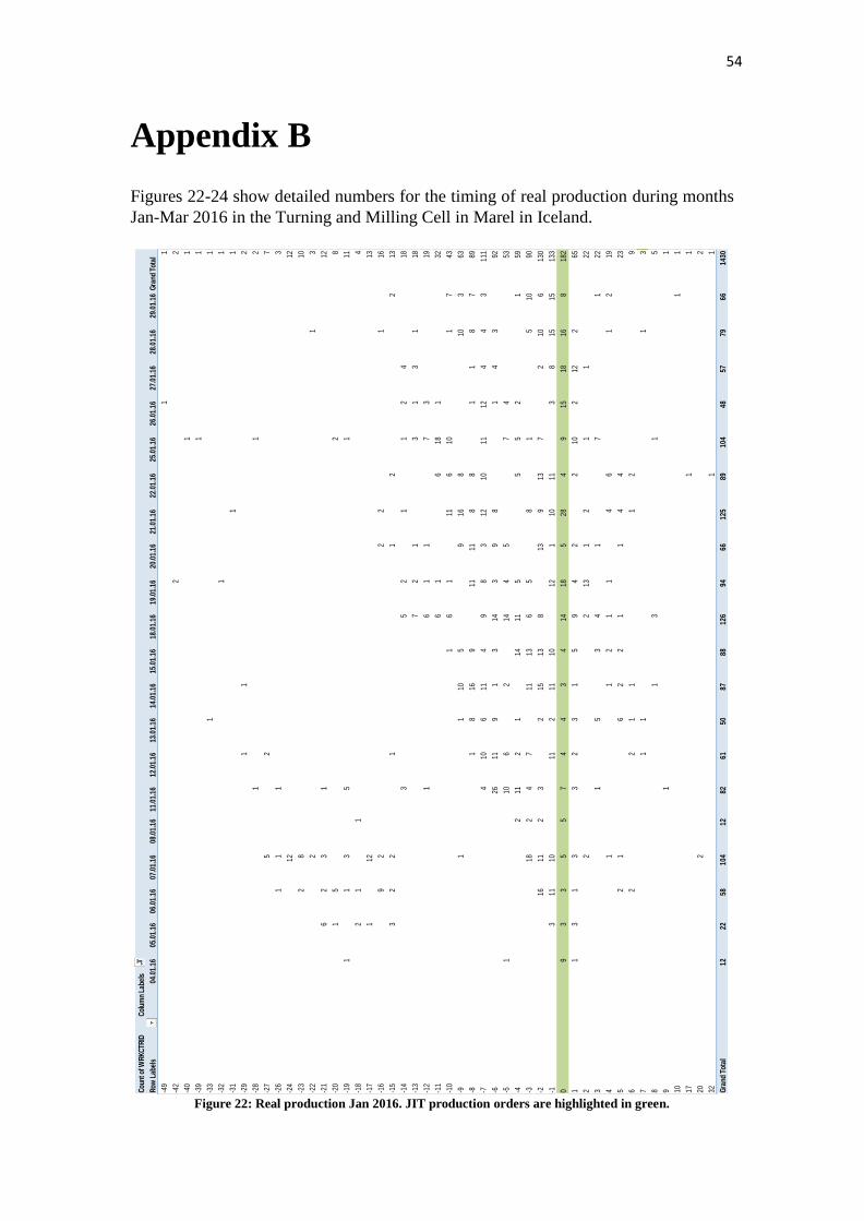
54

Appendix B

Figures 22-24 show detailed numbers for the timing of real production during months

Jan-Mar 2016 in the Turning and Milling Cell in Marel in Iceland.

Figure 22: Real production Jan 2016. JIT production orders are highlighted in green.

Cou

nt o

f WR

KC

TRID

Col

umn

Labe

ls

Row

Lab

els

04.0

1.16

05.0

1.16

06.0

1.16

07.0

1.16

08.0

1.16

11.0

1.16

12.0

1.16

13.0

1.16

14.0

1.16

15.0

1.16

18.0

1.16

19.0

1.16

20.0

1.16

21.0

1.16

22.0

1.16

25.0

1.16

26.0

1.16

27.0

1.16

28.0

1.16

29.0

1.16

Gra

nd T

otal

-49

11

-42

22

-40

11

-39

11

-33

11

-32

11

-31

11

-29

11

2

-28

11

2

-27

52

7

-26

11

13

-24

1212

-23

28

10

-22

21

3

-21

62

31

12

-20

15

28

-19

11

35

111

-18

21

14

-17

112

13

-16

92

22

116

-15

32

21

12

213

-14

35

21

12

418

-13

72

13

13

118

-12

16

11

73

19

-11

61

618

132

-10

16

111

610

17

43

-91

110

59

168

103

63

-81

816

911

118

81

18

789

-74

106

114

98

312

1011

124

43

111

-626

119

13

143

98

14

392

-51

106

214

45

74

53

-42

112

114

115

55

21

59

-318

24

711

136

58

15

1090

-216

112

32

1513

813

913

72

106

130

-13

1110

112

1110

121

1011

38

1515

133

09

33

55

74

43

414

185

284

915

1816

818

2

11

31

33

23

15

94

22

102

122

65

22

213

12

11

22

31

53

41

71

22

41

12

11

46

12

19

52

16

22

11

44

23

62

21

11

29

71

11

3

81

31

5

91

1

101

1

171

1

202

2

321

1

Gra

nd T

otal

1222

5810

412

8261

5087

8812

694

6612

589

104

4857

7966

1430

55

Figure 23: Real production Feb 2016. JIT production orders are highlighted in green.

Row

Lab

els

01.0

2.16

02.0

2.16

03.0

2.16

04.0

2.16

05.0

2.16

08.0

2.16

09.0

2.16

10.0

2.16

11.0

2.16

12.0

2.16

15.0

2.16

16.0

2.16

17.0

2.16

18.0

2.16

19.0

2.16

22.0

2.16

23.0

2.16

24.0

2.16

25.0

2.16

26.0

2.16

Gran

d To

tal

-31

11

-21

44

-20

22

-18

11

-17

13

4

-16

22

15

-15

27

110

-14

12

34

14

116

-13

317

33

55

137

-12

111

311

32

135

150

-11

37

41

112

22

224

159

-10

122

84

52

23

77

64

62

-91

134

51

23

52

14

1051

-818

104

83

25

38

1013

41

82

99

-715

122

610

63

32

31

149

76

24

310

8

-611

2111

46

23

210

229

811

23

412

9

-524

1218

311

46

76

2515

213

3

-410

43

620

29

15

1214

1096

-34

37

122

48

711

218

121

1011

9

-216

88

68

86

217

715

315

1012

9

-19

714

1411

2010

118

3119

2015

18

420

2

021

244

1610

2317

1418

158

1810

513

813

311

525

6

18

91

43

97

25

64

43

93

13

81

24

14

135

42

43

33

46

31

76

11

14

12

24

41

11

43

61

17

52

33

25

21

18

61

32

21

32

11

11

18

73

11

21

8

81

21

4

112

2

121

12

131

1

401

1

Gran

d To

tal

118

128

112

9787

101

9783

6670

5655

133

7212

312

499

1692

6717

96

56

Figure 24: Real production Mar 2016. JIT production orders are highlighted in green.

Co

un

t o

f W

RK

CT

RID

Co

lum

n L

ab

els

Ro

w L

ab

els

29

.02

.16

01

.03

.16

02

.03

.16

03

.03

.16

04

.03

.16

07

.03

.16

08

.03

.16

09

.03

.16

10

.03

.16

11

.03

.16

14

.03

.16

15

.03

.16

16

.03

.16

17

.03

.16

18

.03

.16

21

.03

.16

22

.03

.16

23

.03

.16

24

.03

.16

25

.03

.16

28

.03

.16

29

.03

.16

30

.03

.16

31

.03

.16

Gra

nd

To

tal

-41

11

-38

11

-30

22

-29

22

-25

22

-24

33

-23

22

-22

12

3

-20

11

-19

13

4

-18

22

-17

22

-16

11

2

-15

21

34

21

32

18

-14

22

28

11

12

62

5

-13

32

11

33

15

10

27

91

44

65

-12

22

26

61

21

24

25

27

76

0

-11

41

33

27

44

57

74

7

-10

11

52

81

82

14

61

64

68

-92

15

62

63

35

24

62

62

10

83

-87

85

10

10

55

11

41

08

41

79

54

11

3

-71

12

21

09

65

12

10

36

15

32

42

15

21

37

-61

11

97

78

34

16

47

83

22

21

31

07

-51

55

35

12

27

14

14

29

13

21

12

-42

21

01

25

31

16

73

53

33

75

-33

87

12

18

15

30

22

19

41

22

13

4

-23

14

18

21

92

46

11

31

91

23

41

02

11

16

1

-12

27

51

01

76

14

72

02

81

73

61

17

33

72

20

06

16

62

31

41

32

11

52

21

17

31

31

91

61

21

51

42

34

31

93

94

13

31

35

47

44

25

23

31

91

06

10

2

21

11

33

12

11

14

38

43

32

20

42

22

35

21

12

29

51

22

16

61

11

21

11

19

71

20

15

13

31

82

11

31

19

91

12

10

22

11

11

13

12

11

11

4

13

21

3

14

22

15

11

2

16

11

2

18

11

19

13

4

20

22

24

22

28

11

26

11

Gra

nd

To

tal

50

33

87

10

91

04

86

12

88

98

89

12

12

93

12

01

87

72

57

44

35

62

38

51

06

13

46

72

09

7

57

School of Science and Engineering Reykjavík University Menntavegur 1 101 Reykjavík, Iceland Tel. +354 599 6200 Fax +354 599 6201 www.ru.is

http://www.ru.is/

production scheduling in the tmc in marel iceland

Documents