Project Report: Find the difference! 01/09/2015

Jean FeydyEcole Normale Superieure

jean.feydy@ens.fr

Vincent VidalEcole Normale Superieurevincent.vidal@ens.fr

1. IntroductionWith time, historical monuments may change and –

slightly – evolve: thanks to old paintings or photos, weare able to appreciate it, and point at the differences. Butwhat about computers? This is not a trivial problem at all.Indeed, two different pictures of the “same” building (e.g.a modern photo and an impressionist painting of Notre-Dame) may differ widely, as local textures or small archi-tectural features are left subjects to the artist’s good will.

In this work we shall see how SIFT Features can beused to detect occlusions, architectural deformations anddrawing-errors, the main tool being the “SIFT Flow” algo-rithm proposed in [4].

We shall start in section 2 by giving a brief overview ofthe SIFT Flow algorithm. Then, we will discuss the pos-sibility of using other features than SIFT to compute theoptical flow, before describing in section 3 how the featuresflow can be used to detect occlusions. Eventually, in sec-tion 4, we will present a way to compute a quantitative eval-uation of the distortion – “drawing errors” – for paintingsand drawings.

2. SIFT Flow AlgorithmBasis Algorithm Being given two very different picturesof the same object (e.g. a monument), we would like tofind a dense correspondence map between them, identifyingregions in spite of variations in texture and appearance.

In order to reach this target, we first compute a densefeature field on each image, which gives a local descriptionof every pixel’s neighborhood – SIFT features are used in[4]. Using those features as a measure of similarity, we arethen able to compute a deformation flow w, the “Featureflow”: each pixel p in the first image is identified to thepixel p+wp of the second image. To compute a relevant w,we minimize the following energy function:

E (w) =∑p

‖φ1 (p)− φ2 (p+ wp)‖1

+ γ.∑p

‖wp‖22

+ α.R (w, d)

(1)

0123456789

10

Distortion strengthM

ean

Square

Error

SIFTCNN.3CNN.7Nothing

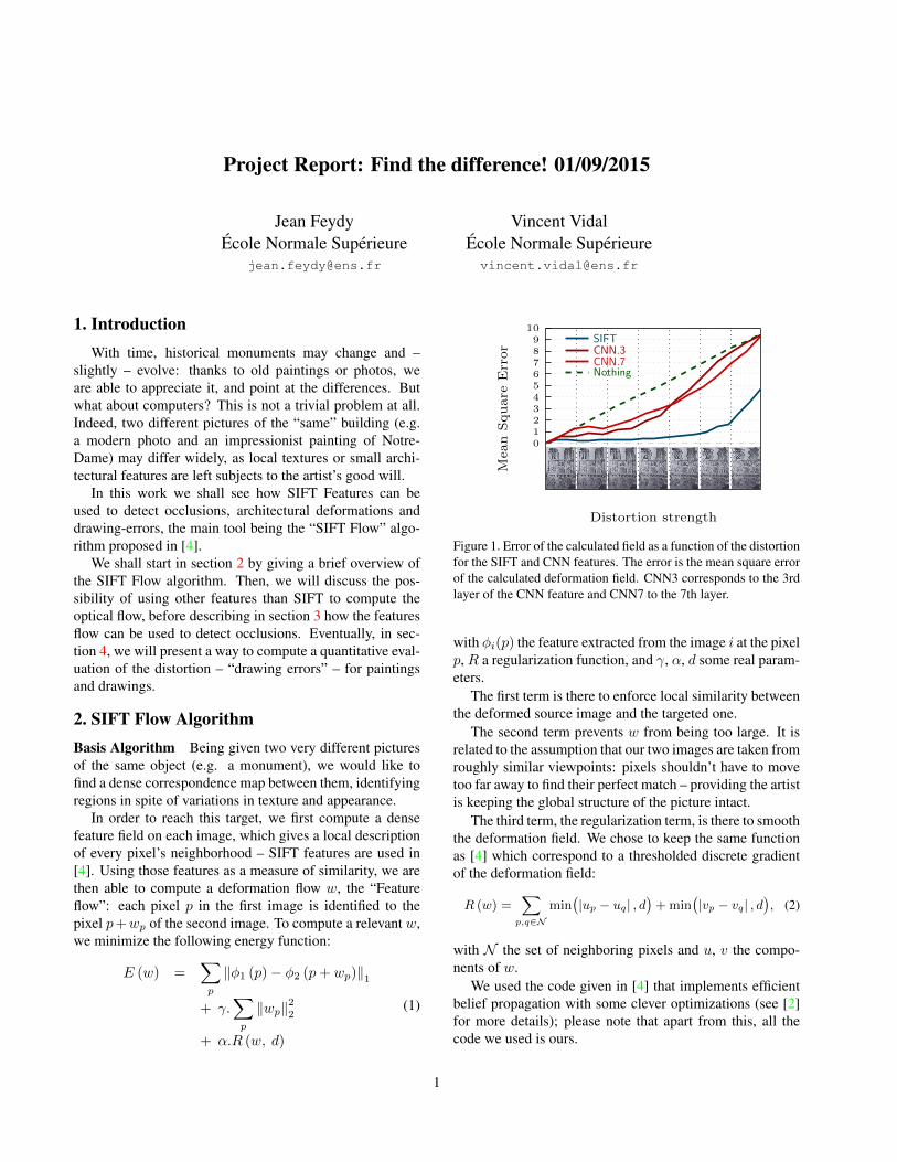
Figure 1. Error of the calculated field as a function of the distortionfor the SIFT and CNN features. The error is the mean square errorof the calculated deformation field. CNN3 corresponds to the 3rdlayer of the CNN feature and CNN7 to the 7th layer.

with φi(p) the feature extracted from the image i at the pixelp, R a regularization function, and γ, α, d some real param-eters.

The first term is there to enforce local similarity betweenthe deformed source image and the targeted one.

The second term prevents w from being too large. It isrelated to the assumption that our two images are taken fromroughly similar viewpoints: pixels shouldn’t have to movetoo far away to find their perfect match – providing the artistis keeping the global structure of the picture intact.

The third term, the regularization term, is there to smooththe deformation field. We chose to keep the same functionas [4] which correspond to a thresholded discrete gradientof the deformation field:

R (w) =∑

p,q∈N

min(|up − uq| , d

)+min

(|vp − vq| , d

), (2)

with N the set of neighboring pixels and u, v the compo-nents of w.

We used the code given in [4] that implements efficientbelief propagation with some clever optimizations (see [2]for more details); please note that apart from this, all thecode we used is ours.

1

Figure 2. From top to bottom, left to right: Reference image,Target image, Method 1 (constrained) result and Method 2 (free-matching) result thresholded so that red corresponds to 10px dis-placement. Notice that the “occlusions” detected on the upper partof Notre-Dame correspond to actual architectural modifications.

Using CNN features A suitable path of improvement ofSIFT flow is the introduction of CNN features. For that pur-pose, we use a “simple” neural network and choose one ofthe layers as the feature’s map feeding the Flow algorithm.

In order to compare the efficiency of the different choicesof features, we take an image, distort it with a known defor-mation v and measure the mean square error of the com-puted field. Figure 1 shows the error curves as a function ofthe distortion for the SIFT and CNN features.

The problem with choosing a layer as feature’s map isthat if we use a layer too deep, the size of the layer’s gridwill be too small and we will lose precision in the deforma-tion field, which explains the bad performances in Figure 1for small deformation, and if we use a shallower layer, theresults are not that good. A good way to do so would be toextract a dense CNN features but a naive approach wouldtake too much time; we would therefore need some deepoptimization, which is the subject of [3].

3. Occlusions detectionThe two strategies We now want to use SIFT flow todetect occlusions in a target image (e.g. an old painting)compared to a reference source image (e.g. a recent, cleanphoto). Our main idea is that occlusions should lead to out-liers in the deformation field, that will be detected simply.

The energy function (eqn. 1) can be written as follows:

E (w) = EFeat + γ.ENorm + α.EReg (d) . (3)

To detect occlusion, we developed two strategies. Thefirst one is to constrain the deformation field to be smooth

and small (γ ∼ 10−3), and detect occlusion by looking atthe first term: “Feature’s Energy”. The second strategy con-sists in lightening the ENorm term (γ ∼ 10−6), so that partsof the objects that are visible in the source image but oc-cluded in the targeted one might be tempted to match otherareas of the picture: in order to minimize the prevailingEFeat, pixels from a brick wall occluded by a tree will tendto match brick regions elsewhere in the picture (which arevery likely to be found) instead of mis-matching with theoccluding foliage texture. We can then detect those move-ments by looking at the “Norm’s Energy”.

Experimentally, the second strategy produces results thatare easier to use for detection purpose (see Figure 2). In-deed, as the first strategy roughly consists in taking the SIFTnorm of the “difference” of the two images – the deforma-tion flow correcting the small irregularities –, occlusions donot lead to plain high energy zones, but to noisy, cloudy ar-eas. After all, the occluding mask may happen to have thesame local aspect as the occluded area once every ten pixels.

Implementation First things first, we have to find param-eters γ, α, d and P that lead to usable ENorm maps – Pis the patchsize of our SIFT descriptors. By hand (trying alarge range of values for every parameter), we chose P = 8,α = 5.10−6, α = 2, d = 2 – some small tuning throughlearning could have been done, but it wouldn’t have lead togroundbreaking improvements as the most meaningful pa-rameter in our case, P , is very constrained.

Without any treatment, sides and corners of our imageare freer to move than its center, as a rectangle image canbe “fold” without introducing any discontinuity. This be-haviour makes little sense in the context of occlusion de-tection, and, instead of modifying the SIFT flow algorithm,we decided to solve this problem by using a framing trick:adding the same 20px-large border frame to the source andtarget image, we tend to fix the borders of the image, thusimposing the same continuity constraint on every pixel.

Eventually, not entirely satisfied by the rough shape ofour occlusion regions (suplevel sets of ENorm), we decidedto combine it with an image segmentation algorithm basedon Mean Shift [1]. Results can be seen in Figure 3, andwould mainly benefit from a more efficient and entirely au-tomatized segmentation technique.

4. Quantitative evaluation

We now want to get a quantitative evaluation of the de-formation between the two images, which can be used tomeasure the accuracy of the representation.

A first way to do so could be to measure the norm of thedeformation field. As we don’t want to include a shiftingpart, we first remove the mean deformation to the deforma-tion field and we don’t want either to consider some occlud-

2

(a) Reference image (b) Occluded image (c) Norm Energy (d) Detected occlusions

Figure 3. Occlusion’s detection using the Norm Energy of SIFT Flow. (a) is the source image. (b) is the occluded target image. (c) is therepresentation of the norm energy (red threshold corresponds to a 10px displacement), with P = 8, α = 5.10−6, α = 2, d = 2. (d) showsthe detected occlusion, obtained by thresholding (c) and applying some segmentation method.

ing objects we need first to remove the occluded part of thedeformation field.

We could also need a more local evaluation of the defor-mation: we want to be able to detect local contraction andextension of the deformation field. In order to get this in-formation, we measure the gradient on a blurred field, to re-duce the noise, and calculate a kind of divergence, as shown

(a) Referenced Image (b) Deformed Picture

(c) Deformation field (d) Deformation label

Figure 4. Painting deformation using SIFT Flow. (a) shows thereferenced image. (b) shows the deformed picture from (a). (c)display the deformation field obtained with the SIFT Flow. (d)shows the divergence of the gradient of the deformation (red cor-responds to dilatation, blue to shrinking).

in Figure 4:

D(w) =∂u

∂x+∂u

∂y+∂v

∂x+∂v

∂ywith w = (u, v) . (4)

We notice that the blur variance parameter corresponds tothe typical scale of the observed deformation.

5. ConclusionWe illustrated here the use of the feature flow algorithm

to solve a non-trivial problem, the comparison of pictures ofa similar scene with a huge variation in rendering style. De-spite obtaining convincing result, we would like to mentionthe work that is still to be done, especially in the dynamicestimation of the scale and segmentation parameters.

References[1] D. Comaniciu and P. Meer. Mean shift: A robust approach

toward feature space analysis. Pattern Analysis and MachineIntelligence, IEEE Transactions on, 24(5):603–619, 2002. 2

[2] P. F. Felzenszwalb and D. P. Huttenlocher. Efficient beliefpropagation for early vision. Int. J. Comput. Vision, 70(1):41–54, Oct. 2006. 1

[3] F. N. Iandola, M. W. Moskewicz, S. Karayev, R. B. Girshick,T. Darrell, and K. Keutzer. Densenet: Implementing efficientconvnet descriptor pyramids. CoRR, abs/1404.1869, 2014. 2

[4] C. Liu, J. Yuen, A. Torralba, J. Sivic, and W. T. Freeman.Sift flow: Dense correspondence across different scenes. InProceedings of the 10th European Conference on ComputerVision: Part III, ECCV ’08, pages 28–42, Berlin, Heidelberg,2008. Springer-Verlag. 1

3