09-07 Project Title: Relating Environmental Conditions to Recruitment and Growth of the Atlantic Sea Scallop (Placopecten magellanicus). Principal Investigators: Burton Shank1, Dvora Hart1, Kevin Friedland2 Contributing Scientists: Grant Law3, Daniel Hennen1

1. Northeast Fisheries Science Center, Woods Hole, MA 2. Northeast Fisheries Science Center, Narragansett, RI 3. Center for Coastal Margin Observation and Prediction, Oregon Health & Science

University, Beaverton, OR Goals:

1. Understand inter-annual variability in recruitment dynamics in the Mid-Atlantic Bight based on environmental or biological factors expected to determine larval supply and early life-history mortality rates. Candidate predictive variables include:

a. Estimated larval supply through calculated spawning stock biomass and potential larval connectivity via the implementation of a larval dispersal model.

b. Coastal phytoplankton blooms as a food supply for pre-spawning brood stock, planktonic larvae, and post-settlement juveniles.

c. Temporal dynamics of benthic invertebrates and demersal fishes that are known scallop predators.

2. Understand inter-annual variability in scallop growth rates by examining appropriate spatial scales of anomalous growth patterns and potential linkages to coastal phytoplankton productivity.

Scope of this report: This report contains a brief description of scallop recruitment dynamics and the work completed to date. The report contains individual section with preliminary results for Goals 1-a, b, and c above. Work on Goal 2 is still in an early phase and is not included in this report. Project timeline: Work on this project began in December 2009. We’ve intentionally spread our effort across the analysis of different datasets in order to screen datasets for promising patterns and allow for lag-times when collaboration with other researchers is necessary. Funding for the first author is expected to continue into January 2011. In the remaining months of this project, we expect to perform further analysis on datasets that are becoming available and write manuscripts as sections of this project solidify. Finally, analyses that prove valuable to understanding or predicting recruitment dynamics will be consolidated into R code modules to allow updated analyses as datasets grow. Introduction Densities of adult sea scallops (Placopecten magellanicus) have increased markedly in the past 15 years in the Mid-Atlantic Bight (MAB) such that fishery catch from the MAB currently is several times that from Georges Bank (GB) which was historically the most productive sea

scallop grounds. High scallop density in the MAB is attributed to an extended period of unusually high recruitment of juvenile scallops combined with improved management (Hart and Rago 2006). Whether or not the increased recruitment is likely to continue (due to e.g., increased spawning stock biomass) or will revert to the lower levels when the environmental regime shifts back to historical norms, is a crucial question for assessment and management of the sea scallop fishery. Scallop larvae disperse in the water column for a period of four to seven weeks before settlement and coastal ocean currents may carry larvae hundreds of kilometers from their spawning ground, making it difficult to predict potential larval supplies for different areas. Also, densities of juvenile scallops are not quantitatively sampled by the NMFS dredge survey until scallops have reached an age of ~2 years. Thus, the observed spatial distribution of juvenile scallops is the result of dispersal patterns coupled with multiple variables: spawning stock fecundity, planktonic survivorship, and post-settlement survivorship acting over a period of a couple years. The central goal of this study is to attempt to quantify the relative contribution of these environmental and biological variables to observed densities of juvenile sea scallops to improve understanding of spatiotemporal variability, improve predictability in population forecasting, and understand how related management actions (fishing activities, ocean zoning) contribute to the population dynamics.

Spatial variation and temporal dynamics of scallop recruitment Inter-annual patterns in juvenile sea scallop density vary spatially. Thus, it was necessary to define sub-regions in the MAB where juvenile density is temporally synchronized. To define these sub-regions (or zones), we first defined a region in the MAB where we judged NMFS dredge surveys were consistently sampled between 1980 and 2009. Using NEFSC sea scallop survey data, we kriged juvenile densities within years across space to a regular grid. We then applied an agglomerative clustering to the predicted densities, using each cell as a sampling unit and each year as a replicate. A trade-off between splitting the MAB into too few sub-regions, which would mask relevant patterns and too many sub-regions, which would potentially complicate analysis and model noise in the dataset, resulted in delineating ten recruitment zones in the MAB, one of which was discontinuous (zone 8) and one of which was subsequently dropped due to insufficient data density (zone 10, Figure 1). Recruitment dynamics in these zones is highly variable among zones, justifying treating the MAB as a set of discontinuous zones rather than a single homogeneous region (Figure 2). Of particular interest, zone 5 shows a remarkable recruitment spike in 2001 and 2002. Goal 1a: Estimation of larval supply from spawning stock biomass and potential larval connectivity via the implementation of a larval dispersal model.

Approach: We estimated larval supply to different areas of the MAB by combining:

1. Survey data on adult sea scallop density and shell height from 1978 – 2009. 2. Statistically-derived relationships between scallop shell height and gonad biomass 3. Estimation of potential larval connectivity using a larval dispersal model.

Work Completed: Estimation of realized larval supply to individual recruitment zones involves calculating spawning stock gonad biomass and potential larval connectivity. We assumed that larval production is proportional to gonad biomass and calculated gonad biomass for all years from individual shell heights using statistical models for the MAB and GB provided by Daniel Hennen. Gonad biomass was then summed across individuals within tows and kriged across the MAB and GB study areas. Potential connectivity matrices for the region were supplied by Grant Law who developed an individual-based sea scallop dispersal model for the region with individual model output for 1980 – 2003. The geographic extent of the model was trimmed to the limits of the study area and potential upstream larval sources (Figure 3). We calculated realized connectivity by combining potential connectivity matrices with calculated gonad biomass and visualized larval connectivity patterns by plotting the resulting realized connectivity matrices (Figure 4). We rescaled realized connectivity to each recruitment zone by spatially sampling the model predictions, weighted by the degree of overlap of the model polygons with the recruitment zone. Resulting predicted larval supplies suggest that zones in the northern Mid-Atlantic and further offshore get the majority of their larvae from Georges Bank while the southern zones in the Mid-Atlantic are seeded by stocks in the northern and central Mid-Atlantic (Figure 5).

Future work: While the calculation of larval supply based on the dispersal model and gonad biomass is instructive, it still does a poor job of predicting the observed spatiotemporal variations in juvenile scallop densities. There are a couple potentially critical parameters we have not yet included in the model that may improve the predictive capacity. We have not included any relationship between gonad biomass and fertilization success which may well be non-linear and affected by small-scale aggregations (10’s or 100’s of meters). Models for the effect of interscallop distance on fertilization success have been developed (Clareboudt 1999, Smith and Rago 2004). It may be possible to use these models with estimates of small-scale spatial variability from the HabCam benthic camera system developed by researchers at Woods Hole Oceanographic Institute, to include the effect of small scale spatial variability in fertilization success. Including fertilization success may be especially important in elucidating the effects of closed areas on larval supply, since sea scallops in closed areas tend to be more aggregated than in fished areas. Food supply may also be a factor in per-capita larval production. Calculations of brood stock food supply may eventually be included in later models, dependent on results from the analysis of coastal phytoplankton densities (Goal 1b). Goal 1b: Coastal phytoplankton blooms as a food supply for pre-spawning brood stock, planktonic larvae, and post-settlement juveniles.

Approach: We hypothesize that food supply during critical early life stages (pre- and post-spawning) may partially determine settlement success and recruitment patterns. Scallops are believed to spawn in the Mid-Atlantic in September and on Georges around October 1 (Hart and Chute 2004). A spring spawn may also occur, especially in the Mid-Atlantic. However, because phytoplankton blooms may affect multiple aspects of scallop reproductive success, the period of time before

and after spawning and the regions where coastal blooms impact recruitment dynamics is difficult to predict. Using satellite-based datasets (SeaWiFS and MODIS) of coastal chlorophyll concentration from 1998 – 2007, we first screened the data for patterns of general correlations between inter-annual fluctuations in chlorophyll concentration and recruitment densities. Based on this, we defined discrete regions and time periods that we hypothesize are potentially linked to recruitment dynamics and examine the capacity for data from these regions to effectively predict fluctuations in recruitment.

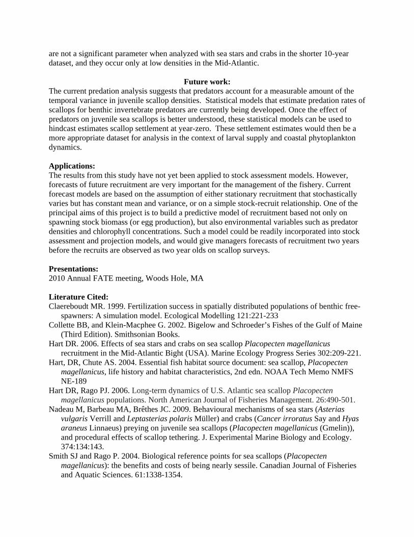
Work Completed: We examined correlations between chlorophyll concentrations and recruitment dynamics using Partial Least Squares analysis. We examined all models for all zones using average chlorophyll densities at half-degree resolution across time periods of eight to 64 days, ending between August 4th and October 31st. We plotted the resulting fit of each model on a surface to examine patterns in model fit for different sample periods and the loadings of chlorophyll from each geographic cell to determine when and where chlorophyll blooms have an apparent relationship with recruit densities. Plots of model results commonly suggest sample periods of 32 to 40 days in length with end dates in late September for zones that recruit from within the Mid-Atlantic and end dates in early or mid-October (see example Figure 6) for zones that tend to recruit from Georges Bank. Resulting maps tended to identify two specific regions where chlorophyll potentially influences recruitment dynamics, one off the coast of New Jersey and one more or less centered on Georges Bank (Figure 7). From this analysis, we initially select different regions and time periods for further analysis: one region off New Jersey with a 32-day time period ending in mid-September and one region on Georges Bank, also with a 32-day time period but ending in mid-October, both 1.5 square degrees in area. We then examined the degree to which average chlorophyll from these regions and time periods predict recruitment in each zone. Chlorophyll densities from both of the selected regions are statistically correlated with juvenile densities in both zone 2 and zone 5 (Figure 8). However, preliminary analysis does not indicate that chlorophyll from these two regions is a significant predictor of juvenile densities in the other zones.

Future work: It is apparent that chlorophyll levels alone are potentially predictive of recruitment dynamics in the Mid-Atlantic, at least in some regions. However, the selection of discrete regions as sources of food for pre-spawning or larval-stage scallops, though useful for explaining some of the anomalously high recruitment events, is both subjective and of limited application across this region. We anticipate combining the chlorophyll dataset with the larval supply model to create a more fully parameterized model of larval production and dispersal. Because satellite data give chlorophyll densities on the surface whereas scallops feed in the benthos, chlorophyll data may be a better indicator of food supply for planktonic larvae than of carbon flux to the brood stock. Variability in chlorophyll densities and the existence of shelf fronts may be a better indicator of benthic carbon flux than mean surface chlorophyll.

Goal 1c: Predation effects of benthic invertebrates and demersal fishes on juvenile sea scallops.

Approach: Predation on juvenile sea scallops is a potentially important process structuring scallop densities (Hart 2006, Nadeau et al. 2009). We look for evidence of predators influencing juvenile densities of sea scallops by examining temporal synchrony between scallop densities and densities of benthic invertebrate and demersal fish predators. The primary dataset contains densities of three known benthic invertebrate predators that are common in sea scallop habitats in the Mid-Atlantic; the sea stars Asterias spp. and Astropecten americanus, and Cancer crabs. Data on these three groups have been collected as a part of NMFS dredge survey since 2000. Predator densities vary temporally and there may be a temporal lag between the life history stage when predators are actually consuming juvenile sea scallops and the sampling of predators and sea scallops. Thus, we estimate predator densities at time lags of up to two years prior to sampling and examine if temporal fluctuation in juvenile scallop densities correlate with fluctuations in predator densities. A secondary dataset contains densities of American lobster (Homarus americanus) and demersal fishes that have been recorded to prey on sea scallops. This dataset is taken from the NMFS trawl survey from 1980 – 2009 and similarly interpolated to dredge survey locations and examined for temporal synchrony.

Work Completed: We initially examined temporal synchrony in predator / sea scallop densities by grouping the study area into half-degree regions and analyzing temporal dynamics within each region. Having detected robust negative relationships between two of the predators (Astropecten and Cancer), we re-scaled the spatial regions to the recruitment zones and re-analyzed. Similar negative relationships between predator and prey densities were found for the recruitment zones with Cancer crabs showing a variable effect across the zones (Figure 9). The estimated slope coefficient for Cancer is steeper than the slope for Astropecten, suggesting that the crabs have a higher per-capita predation rate. However, densities of Astropecten sea stars in the Mid-Atlantic are much higher than crabs (Figure 10), so both species have potentially large impacts on scallop populations. Scallop recruitment is negatively correlated with predator densities in all zones, and the combined effects of the two predators significantly predict juvenile scallop densities in zone 2 and 5 and account for a trend in zone 6 (Figure 11). To analyze the 30-year dataset of predators from the bottom trawl database, we first detrended all predator populations as well as sea stars. After detrending, two demersal fishes were significantly related with sea star dynamics: winter flounder (Pseudopleuronectes americanus) which were associated with year-two scallops (p=0.0002), and ocean pout (Zoarces americanus) which were associated with year-one scallops (p=0.005). Molluscs make up a very small portion of the diet of winter flounder (Collette and Klein-Macphee 2002) and their gape is probably too small to effectively eat year-two scallops (25mm+) so the observed relationship between winter flounder and sea scallops is probably the result of both species responding to an environmental variable rather than a predatory/prey relationship. Sea scallops are a known dietary constituent of ocean pout so this observed relationship is potentially worth retaining. However, ocean pout

are not a significant parameter when analyzed with sea stars and crabs in the shorter 10-year dataset, and they occur only at low densities in the Mid-Atlantic.

Future work: The current predation analysis suggests that predators account for a measurable amount of the temporal variance in juvenile scallop densities. Statistical models that estimate predation rates of scallops for benthic invertebrate predators are currently being developed. Once the effect of predators on juvenile sea scallops is better understood, these statistical models can be used to hindcast estimates scallop settlement at year-zero. These settlement estimates would then be a more appropriate dataset for analysis in the context of larval supply and coastal phytoplankton dynamics. Applications: The results from this study have not yet been applied to stock assessment models. However, forecasts of future recruitment are very important for the management of the fishery. Current forecast models are based on the assumption of either stationary recruitment that stochastically varies but has constant mean and variance, or on a simple stock-recruit relationship. One of the principal aims of this project is to build a predictive model of recruitment based not only on spawning stock biomass (or egg production), but also environmental variables such as predator densities and chlorophyll concentrations. Such a model could be readily incorporated into stock assessment and projection models, and would give managers forecasts of recruitment two years before the recruits are observed as two year olds on scallop surveys. Presentations: 2010 Annual FATE meeting, Woods Hole, MA Literature Cited: Claereboudt MR. 1999. Fertilization success in spatially distributed populations of benthic free- spawners: A simulation model. Ecological Modelling 121:221-233 Collette BB, and Klein-Macphee G. 2002. Bigelow and Schroeder’s Fishes of the Gulf of Maine

(Third Edition). Smithsonian Books. Hart DR. 2006. Effects of sea stars and crabs on sea scallop Placopecten magellanicus

recruitment in the Mid-Atlantic Bight (USA). Marine Ecology Progress Series 302:209-221. Hart, DR, Chute AS. 2004. Essential fish habitat source document: sea scallop, Placopecten

magellanicus, life history and habitat characteristics, 2nd edn. NOAA Tech Memo NMFS NE-189 Hart DR, Rago PJ. 2006. Long-term dynamics of U.S. Atlantic sea scallop Placopecten

magellanicus populations. North American Journal of Fisheries Management. 26:490-501. Nadeau M, Barbeau MA, Brêthes JC. 2009. Behavioural mechanisms of sea stars (Asterias

vulgaris Verrill and Leptasterias polaris Müller) and crabs (Cancer irroratus Say and Hyas araneus Linnaeus) preying on juvenile sea scallops (Placopecten magellanicus (Gmelin)), and procedural effects of scallop tethering. J. Experimental Marine Biology and Ecology. 374:134:143.

Smith SJ and Rago P. 2004. Biological reference points for sea scallops (Placopecten magellanicus): the benefits and costs of being nearly sessile. Canadian Journal of Fisheries and Aquatic Sciences. 61:1338-1354.

Figure 1. Mean juvenile sea scallop density 1978 – 2007. Color indicates density (# juveniles / survey tow). Polygons represent recruitment zones, derived from cluster analysis, where juvenile dynamics are temporally synchronized. Zone 10 was excluded from further analysis due to insufficient sample size.

Figure 2. Temporal dynamics of juvenile sea scallops in the nine recruitment zones: (a) linear scale with a common Y-axis for all subplots, (b) log-scaled with different Y-axes for each recruitment zone. Zones are labeled in the strip to the left of each plot. Dotted black and dashed red lines indicate the beginnings of the satellite chlorophyll and invertebrate predator datasets respectively.

Figure 3. Geographic extent of the original larval dispersal model and the portion of the model included in the study area (numbered cells). Retained geographic regions include: DMV – DelMarVa, ET – Elephant Trunk, HC – Hudson Canyon, NMA – Northern Mid-Atlantic, LSR – Nantucket Lightship Region, and GB – Georges Bank.

Figure 4. Example log-scaled realized connectivity matrices for 1998 – 2003. Yellow indicates a large larval supply while dark colors indicate small or no larval supply. Sinks are in rows where sources are in columns; rows indicate where larvae for a location came from while columns indicate where larvae from a location went to. Regions (MAB vs. GB) are divided by the solid line while subregions are divided by a dashed line. Subregions are DMV – DelMarVa, ET – Elephant Trunk, HC – Hudson Canyon, NMA – Northern Mid-Atlantic, LSR – Nantucket Lightship Region, GB – Georges Bank.

Figure 5. Modeled larval supply for recruitment zones in the Mid-Atlantic. Filled blue and open black markers indicate MAB and GB sources, respectively. Triangular markers represent year-specific model predictions while circular markers represent an average potential connectivity model with year-varying gonad biomass.

Figure 6. Surface of model fits for different sampling durations and end dates from the chlorophyll dataset. Plotted results are the R-square for the first PLS latent variable on recruitment dynamics in recruitment zone 5 for 1999 – 2007. From such plots, we selected sampling period lengths and end dates that provided good fits to the data but with moderate length time periods that were more probable to retain predictive capacity with the addition of new data.

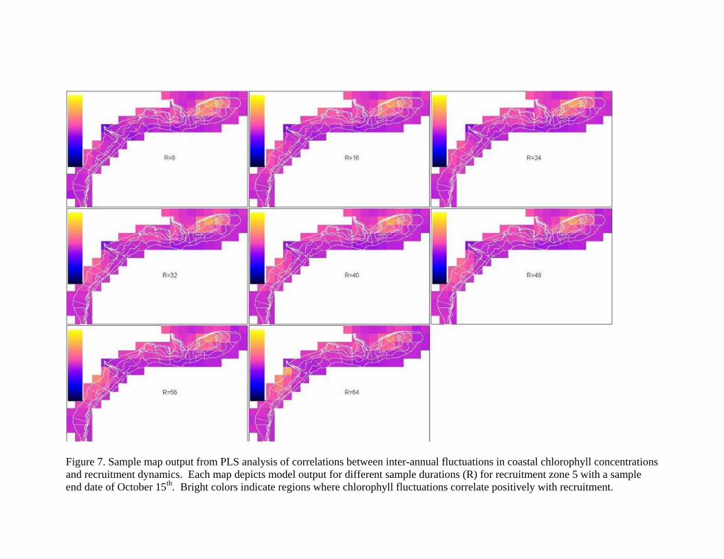
Figure 7. Sample map output from PLS analysis of correlations between inter-annual fluctuations in coastal chlorophyll concentrations and recruitment dynamics. Each map depicts model output for different sample durations (R) for recruitment zone 5 with a sample end date of October 15th. Bright colors indicate regions where chlorophyll fluctuations correlate positively with recruitment.

Figure 8. Correlation between average chlorophyll concentrations (x – axis) in the Mid-Atlantic (A) and Georges Bank (B) and scallop recruit densities in the Mid-Atlantic for 1999 – 2007. Statistically-significant relationships are shown in red with p-values listed.

Figure 9. Temporal correlation between Astropecten and Cancer predator densities and juvenile scallop densities. Top figures estimate a common predator/prey relationship for all recruitment zones. Bottom figures estimate separate predator/prey relationships for each recruitment zone.

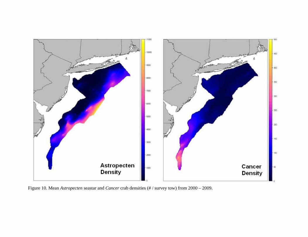
Figure 10. Mean Astropecten seastar and Cancer crab densities (# / survey tow) from 2000 – 2009.

Figure 11. Effect of predator density fluctuations on densities of juvenile scallops. For the model scallop density ~ sea star density + crab density, the x-axis is predicted values from the model while the y-axis is actual scallop densities. Significant relationships (p<0.05) are shown with a red trendline while trends (p<0.10) are shown with a blue line.