projection-based methods in optimization
TRANSCRIPT

Projection-Based Methods in Optimization
Charles Byrne(Charles [email protected])
http://faculty.uml.edu/cbyrne/cbyrne.htmlDepartment of Mathematical Sciences
University of Massachusetts LowellLowell, MA 01854, USA
June 3, 2013

Talk Available on Web Site
This slide presentation and accompanying article are availableon my web site, http://faculty.uml.edu/cbyrne/cbyrne.html ; clickon “Talks”.

Using Prior Knowledge
Figure : Minimum Two-Norm and Minimum Weighted Two-NormReconstruction.

Fourier Transform as Data
Figure : Far-field Measurements. The distance from x to P isapproximately D − x cos θ.
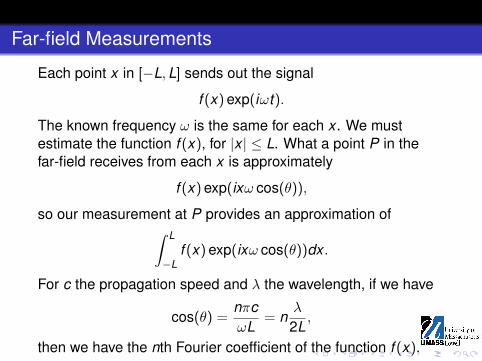
Far-field Measurements
Each point x in [−L,L] sends out the signal
f (x) exp(iωt).
The known frequency ω is the same for each x . We mustestimate the function f (x), for |x | ≤ L. What a point P in thefar-field receives from each x is approximately
f (x) exp(ixω cos(θ)),
so our measurement at P provides an approximation of∫ L
−Lf (x) exp(ixω cos(θ))dx .
For c the propagation speed and λ the wavelength, if we have
cos(θ) =nπcωL
= nλ
2L,
then we have the nth Fourier coefficient of the function f (x).

The Limited-Data Problem
We can havecos(θ) =
nπcωL
= nλ
2Lonly if
|n| ≤ 2Lλ,
so we can measure only a limited number of the Fouriercoefficients of f (x). Note that the upper bound on |n| is thelength of the interval [−L,L] in units of wavelength.
Can We Get More Data?
Clearly, we can take our measurements at any point P on thecircle, not just at those satisfying the equation
cos(θ) =nπcωL
= nλ
2L.
These measurements provide additional information about f (x),but won’t be additional Fourier coefficients for the Fourier seriesof f (x) on [−L,L]. How can we use these additionalmeasurements to improve our estimate of f (x)?

Over-Sampled Data
Suppose that we over-sample; let us take measurements atpoints P such that the associated angle θ satisfies
cos(θ) =nπcωKL
,
where K > 1 is a positive integer, instead of
cos(θ) =nπcωL
.
Now we have Fourier coefficients for the function g(x) that isf (x) for |x | ≤ L, and is zero on the remainder of the interval[−KL,KL].

Using Support Information
Given our original limited data, we can calculate the orthogonalprojection of the zero function onto the subset of all functionson [−L,L] consistent with this data; this is the minimum-normestimate of f (x), also called the discrete Fourier transform(DFT) estimate, shown in the second graph below.If we use the over-sampled data as Fourier coefficients for g(x)on the interval [−KL,KL], we find that we haven’t improved ourestimate of f (x) for |x | ≤ L.Instead, we calculate the orthogonal projection of the zerofunction onto the subset of all functions on [−L,L] that areconsistent with the over-sampled data. This is sometimescalled the modified DFT (MDFT) estimate. The top graph belowshows the MDFT for a case of K = 30.
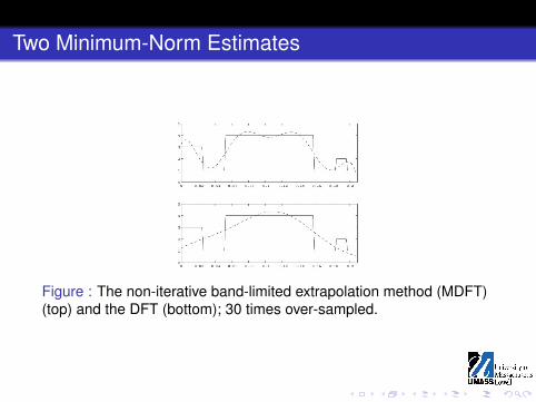
Two Minimum-Norm Estimates
Figure : The non-iterative band-limited extrapolation method (MDFT)(top) and the DFT (bottom); 30 times over-sampled.

Over-Sampled Fourier-Transform Data
For the simulation in the figure above, f (x) = 0 for |x | > L. Thetop graph is the minimum-norm estimator, with respect to theHilbert space L2(−L,L), called the modified DFT (MDFT); thebottom graph is the DFT, the minimum-norm estimator withrespect to the Hilbert space L2(−30L,30L), shown only for[−L,L]. The MDFT is a non-iterative variant ofGerchberg-Papoulis band-limited extrapolation.

Using Orthogonal Projection
In both of the examples above we see minimum two-normsolutions consistent with the data. These reconstructionsinvolve the orthogonal projection of the zero vector onto the setof solutions consistent with the data. The improvementsillustrate the advantage gained by the selection of anappropriate ambient space within which to perform theprojection. The constraints of data consistency define a subsetonto which we project, and the distance to zero is the functionbeing minimized, subject to the constraints. This leads to themore general problem of optimizing a function, subject toconstraints.

The Basic Problem
The basic problem we consider here is to minimize areal-valued function
f : X → R,
over a subset C ⊆ X , where X is an arbitrary set. With
ιC(x) = 0, for x ∈ C, and +∞, otherwise,
we can rewrite the problem as minimizing f (x) + ιC(x), over allx ∈ X .

The Limited-Data Problem
We want to reconstruct or estimate a function of severalcontinuous variables. We have limited noisy measured dataand some prior information that serve to constrain that function.We discretize the function, so that the object is described as anunknown vector x in RJ .

Constraints
We want our reconstruction to be at least approximatelyconsistent with the measured data. We may know that theentries of x are non-negative. When x is a vectorized image,we may have prior knowledge of its general appearance (ahead slice, for example). If x is an extrapolated band-limitedtime series, we may have prior knowledge of the extent of theband.

Representing Constraints
Prior knowledge of general properties of x can be incorporatedthrough the choice of the ambient space. Other constraints,such as the measured data, tell us that x lies in a subset C ofthe ambient space.

An Example: Linear Functional Data
Suppose that the measured data vector b is linear in x , withAx = b under-determined. The minimum two-norm solutionminimizes
J∑j=1
|xj |2,
subject to Ax = b. Let the vector p with entries pj > 0 be a priorestimate of the magnitudes |xj |. The minimum weightedtwo-norm solution minimizes
J∑j=1
|xj |2/pj ,
subject to Ax = b.

Using Optimization
When the constraint set C is relatively small, any member of Cmay provide an adequate solution to the problem. More likely,C is relatively large, and we may choose to determine x byminimizing a cost function over the set C.
An Example- Systems of Linear Equations
Let the data b pertaining to x be linear, so that Ax = b for somematrix A.
1. When there are infinitely many solutions, we may selectx to minimize a norm or other suitable distance measure;2. When there are no solutions, we may select aleast-squares or other approximate solution;3. When the data b is noisy, we may select a regularizedsolution.

Barrier Functions: An Example
The problem is to minimize the function
f (x) = f (x1, x2) = x21 + x2
2 , subject to x1 + x2 ≥ 1.
For each positive integer k , the vector xk with entries
xk1 = xk
2 =14
+14
√1 +
4k
minimizes the function
Bk (x) = x21 + x2
2 −1k
log(x1 + x2 − 1) = f (x) +1k
b(x).
Notice that xk1 + xk
2 > 1, so each xk satisfies the constraint. Ask → +∞, xk converges to (1
2 ,12), which solves the original
problem.

Penalty Functions: An Example
The problem is to minimize the function
f (x) = (x + 1)2, subject to x ≥ 0.
Our penalty function is
p(x) = x2, for x ≤ 0, p(x) = 0, for x > 0.
At the k th step we minimize
f (x) + kp(x)
to get xk = −1k+1 , which converges to the right answer, x∗ = 0,
as k →∞. The limit x∗ satisfies the constraint, but the xk donot; this is an exterior-point method.
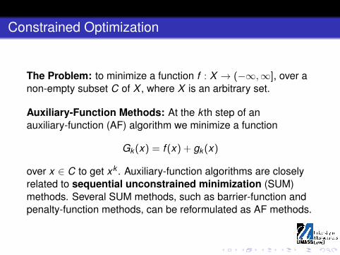
Constrained Optimization
The Problem: to minimize a function f : X → (−∞,∞], over anon-empty subset C of X , where X is an arbitrary set.
Auxiliary-Function Methods: At the k th step of anauxiliary-function (AF) algorithm we minimize a function
Gk (x) = f (x) + gk (x)
over x ∈ C to get xk . Auxiliary-function algorithms are closelyrelated to sequential unconstrained minimization (SUM)methods. Several SUM methods, such as barrier-function andpenalty-function methods, can be reformulated as AF methods.
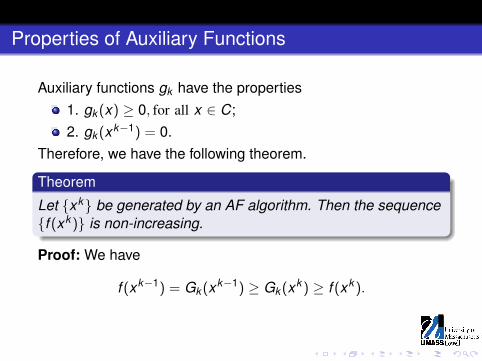
Properties of Auxiliary Functions
Auxiliary functions gk have the properties1. gk (x) ≥ 0, for all x ∈ C;2. gk (xk−1) = 0.
Therefore, we have the following theorem.
Theorem
Let {xk} be generated by an AF algorithm. Then the sequence{f (xk )} is non-increasing.
Proof: We have
f (xk−1) = Gk (xk−1) ≥ Gk (xk ) ≥ f (xk ).
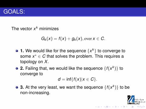
GOALS:
The vector xk minimizes
Gk (x) = f (x) + gk (x), over x ∈ C.
1. We would like for the sequence {xk} to converge tosome x∗ ∈ C that solves the problem. This requires atopology on X .2. Failing that, we would like the sequence {f (xk )} toconverge to
d = inf{f (x)|x ∈ C}.
3. At the very least, we want the sequence {f (xk )} to benon-increasing.

SUMMA
An AF algorithm in said to be in the SUMMA class if
Gk (x)−Gk (xk ) ≥ gk+1(x) ≥ 0,
for all x ∈ C.
Theorem
For algorithms in the SUMMA class, the sequence {f (xk )} isnon-increasing, and we have
{f (xk )} ↓ d = inf{f (x)|x ∈ C}.

SUMMA Proof:
If f (xk ) ≥ d∗ > f (z) ≥ d for all k , then
gk (z)− gk+1(z) ≥ gk (z)− (Gk (z)−Gk (xk ))
= f (xk )− f (z) + gk (xk ) ≥ d∗ − f (z) > 0.
But the decreasing non-negative sequence {gk (z)} cannothave its successive differences bounded away from zero.
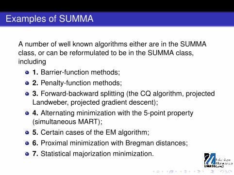
Examples of SUMMA
A number of well known algorithms either are in the SUMMAclass, or can be reformulated to be in the SUMMA class,including
1. Barrier-function methods;2. Penalty-function methods;3. Forward-backward splitting (the CQ algorithm, projectedLandweber, projected gradient descent);4. Alternating minimization with the 5-point property(simultaneous MART);5. Certain cases of the EM algorithm;6. Proximal minimization with Bregman distances;7. Statistical majorization minimization.

Barrier-Function Methods
A function b : C → [0,+∞] is a barrier function for C, that is, bis finite on C, b(x) = +∞, for x not in C, and, for topologized X ,has the property that b(x)→ +∞ as x approaches theboundary of C. At the k th step of the iteration we minimize
f (x) +1k
b(x)
to get xk . Equivalently, we minimize
Gk (x) = f (x) + gk (x),
with
gk (x) = [(k − 1)f (x) + b(x)]− [(k − 1)f (xk−1) + b(xk−1)].
ThenGk (x)−Gk (xk ) = gk+1(x).

Penalty-Function Methods
We select a non-negative function p : X → R with the propertythat p(x) = 0 if and only if x is in C and then, for each positiveinteger k , we minimize
f (x) + kp(x),
or, equivalently,
p(x) +1k
f (x),
to get xk . Most, but not all, of what we need concerningpenalty-function methods can then be obtained from thediscussion of barrier-function methods.

Bregman Distances
Let f : Z ⊆ RJ → R be convex on its domain Z , anddifferentiable on the interior U of Z . For x ∈ Z and y ∈ U, theBregman distance from y to x is
Df (x , y) = f (x)− f (y)− 〈∇f (y), x − y〉.
Then, because of the convexity of f , Df (x , y) ≥ 0 for all x and y .
The Euclidean distance is the Bregman distance for
f (x) =12‖x‖22.
Proximal Minimization Algorithms (PMA)
Let f : C ⊆ RJ → R be convex on C and differentiable on theinterior U of C. At the k th step of a proximal minimization (proxmin) algorithm (PMA), we minimize the function
Gk (x) = f (x) + Dh(x , xk−1),
to get xk . The function gk (x) = Dh(x , xk−1) is the Bregmandistance associated with the Bregman function h. We assumethat each xk lies in U, whose closure is the set C. We have
Gk (x)−Gk (xk ) = Df (x , xk ) + Dh(x , xk ) ≥ Dh(x , xk ) = gk+1(x).

Another Job for the PMA
Suppose that
f (x) =12‖Ax − b‖22,
with AAT invertible. If the PMA sequence {xk} converges tosome x∗ and ∇h(x0) is in the range of AT then x∗ minimizesh(x) over all x with Ax = b.

Obstacles in the PMA
To obtain xk in the PMA we must solve the equation
∇f (xk ) +∇h(xk ) = ∇h(xk−1).
This is usually not easy. However, we can modify the PMA toovercome this obstacle. This modified PMA is an interior-pointalgorithm that we have called the IPA.
The IPA
We still get xk by minimizing
Gk (x) = f (x) + Dh(x , xk−1).
Witha(x) = h(x) + f (x),
we find that xk solves
∇a(xk ) = ∇a(xk−1)−∇f (xk−1).
Therefore, we look for a(x) so that1. h(x) = a(x)− f (x) is convex;2. obtaining xk from ∇a(xk ) is easy now.

The IPA and Constraints
In the PMA, h can be chosen to force xk to be in U, the interiorof the domain of h. In the IPA it is a(x) that we select, andincorporating the constraints within a(x) may not be easy.

The Projected Landweber Algorithm as IPA
We want to
minimize f (x) =12‖Ax − b‖22, over x ∈ C.
We select γ so that 0 < γ < 1ρ(AT A) and
a(x) =1
2γ‖x‖22.
We haveDf (x , y) =
12‖Ax − Ay‖22,
and we minimize
Gk (x) = f (x) +1
2γ‖x − xk−1‖22 −
12‖Ax − Axk−1‖22
over x in C to get
xk = PC(xk−1 − γAT (Axk−1 − b)).

An Example of the IPA: Projected Gradient Descent
Let f be convex and differentiable on RJ , with ∇f L-Lipschitz,and 0 < γ ≤ 1
L . Let C ⊆ RJ be closed, nonempty, and convex.Let
a(x) =1
2γ‖x‖22.
At the k th step we minimize
Gk (x) = f (x) +1
2γ‖x − xk−1‖22 − Df (x , xk−1),
over x ∈ C, obtaining
xk = PC(xk−1 − γ∇f (xk−1));
PC is the orthogonal projection onto C.

Projected Gradient Descent as SUMMA
The auxiliary function gk (x) can be written as
gk (x) =1
2γ‖x − xk−1‖22 − Df (x , xk−1) = Dh(x , xk−1),
where h(x) is the convex differentiable function
h(x) = a(x)− f (x) =1
2γ‖x‖22 − f (x).
Then
Gk (x)−Gk (xk ) = Da(x , xk ) ≥ Dh(x , xk ) = gk+1(x).

Majorization Minimization or Optimization Transfer
Majorization minimization or optimization transfer is used instatistical optimization.
For each fixed y , let g(x |y) ≥ f (x), for all x , and g(y |y) = f (y).At the k th step we minimize g(x |xk−1) to get xk . This statisticalmethod is equivalent to minimizing
f (x) + D(x , xk−1) = f (x) + gk (x),
wheregk (x) = D(x , xk−1),
for some distance measure D(x , z) ≥ 0, with D(z, z) = 0.

The Method of Auslander and Teboulle
The method of Auslander and Teboulle is a particular exampleof an MM method that is not in SUMMA. At the k th step of theirmethod
minimize Gk (x) = f (x) + D(x , xk−1) to get xk .
They assume that D has an associated induced proximaldistance H(a,b) ≥ 0, finite for a and b in C, with H(a,a) = 0and
〈∇1d(b,a), c − b〉 ≤ H(c,a)− H(c,b),
for all c in C. Here ∇1D(x , y) denotes the x gradient. We dohave {f (xk )} → d . If D = Dh, then H = Dh also; Bregmandistances are self-proximal.

Projected Gradient Descent (PGD) Revisited
At the k th step of the PGD we minimize
Gk (x) = f (x) +1
2γ‖x − xk−1‖22 − Df (x , xk−1),
over x ∈ C. Equivalently, we minimize the function
ιC(x) + f (x) +1
2γ‖x − xk−1‖22 − Df (x , xk−1),
over all x in RJ , with ιC(x) = 0 for x ∈ C and ιC(x) = +∞otherwise. Now the objective function is a sum of two functions,one non-differentiable. The forward-backward splitting methodthen applies.

Moreau’s Proximity Operators
Let f : RJ → R be convex. For each z ∈ RJ the function
mf (z) := minx{f (x) +
12‖x − z‖22}
is minimized by a unique x = proxf (z). Moreau’s proximityoperator proxf extends the notion of orthogonal projection ontoa closed convex set: if f (x) = ιC(x) then proxf (x) = PC(x). Also
x = proxf (z) iff z − x ∈ ∂f (x) iff x = J∂f (z),
where J∂f (z) is the resolvent of the set-valued operator ∂f .

Forward-Backward Splitting
Let f : RJ → R be convex, with f = f1 + f2, both convex, f2differentiable, and ∇f2 L-Lipschitz continuous. The iterative stepof the FBS algorithm is
xk = proxγf1
(xk−1 − γ∇f2(xk−1)
),
which can be obtained by minimizing
Gk (x) = f (x) +1
2γ‖x − xk−1‖22 − Df2(x , xk−1).
Convergence of the sequence {xk} to a solution can beestablished, if γ is chosen to lie within the interval (0,1/L].

Projected Gradient Descent as FBS
To put the projected gradient descent method into theframework of the forward-backward splitting we let
f1(x) = ιC(x),
the indicator function of the set C, which is zero for x ∈ C and+∞ otherwise. Then we minimize the function
f1(x) + f2(x) = ιC(x) + f (x)
over all x ∈ RJ .

The CQ Algorithm
Let A be a real I by J matrix, C ⊆ RJ , and Q ⊆ RI , both closedconvex sets. The split feasibility problem (SFP) is to find x inC such that Ax is in Q. The function
f2(x) =12‖PQAx − Ax‖22
is convex and differentiable, ∇f2 is ρ(AT A)-Lipschitz, and
∇f2(x) = AT (I − PQ)Ax .
We want to minimize the function f (x) = ιC(x) + f2(x), over allx . The FBS algorithm gives the iterative step for the CQalgorithm; with 0 < γ ≤ 1/L,
xk = PC
(xk−1 − γAT (I − PQ)Axk−1
).

Alternating Minimization
Suppose that P and Q are arbitrary non-empty sets and thefunction Θ(p,q) satisfies −∞ < Θ(p,q) ≤ +∞, for each p ∈ Pand q ∈ Q.The general AM method proceeds in two steps: we begin withsome q0, and, having found qk−1, we
1. minimize Θ(p,qk−1) over p ∈ P to get p = pk , and then2. minimize Θ(pk ,q) over q ∈ Q to get q = qk .
The 5-point property of Csiszár and Tusnády is
Θ(p,q) + Θ(p,qk−1) ≥ Θ(p,qk ) + Θ(pk ,qk−1).

AM as SUMMA
When the 5-point property holds for AM, the sequence{Θ(pk ,qk )} converges to
d = infp,q
Θ(p,q).
For each p ∈ P, define q(p) to be some member of Q for whichΘ(p,q(p)) ≤ Θ(p,q), for all q ∈ Q; then q(pk ) = qk . Define
f (p) = Θ(p,q(p)).
At the k th step of AM we minimize
Gk (p) = Θ(p,qk−1) = f (p) + gk (p),
wheregk (p) = Θ(p,qk−1)−Θ(p,q(p)).
The 5-point property is then the SUMMA condition
Gk (p)−Gk (pk ) ≥ gk+1(p) ≥ 0.

Kullback-Leibler Distances
For a > 0 and b > 0, the Kullback-Leibler distance from a tob is
KL(a,b) = a log a− a log b + b − a,
with KL(0,b) = b, and KL(a,0) = +∞. The KL distance isextended to non-negative vectors entry-wise.
Let y ∈ RI be positive, and P an I by J matrix with non-negativeentries. The simultaneous MART (SMART) algorithmminimizes KL(Px , y), and the EMML algorithm minimizesKL(y ,Px), both over all non-negative x ∈ RJ . Both algorithmscan be viewed as particular cases of alternating minimization.

The General EM Algorithm
The general EM algorithm is essentially non-stochastic. Let Zbe an arbitrary set. We want to maximize
L(z) =
∫b(x , z)dx , over z ∈ Z ,
where b(x , z) : RJ × Z → [0,+∞]. Given zk−1, we takef (z) = −L(z) and
minimize Gk (z) = f (z) +
∫KL(b(x , zk−1),b(x , z))dx to get zk .
Sincegk (z) =
∫KL(b(x , zk−1),b(x , z))dx ≥ 0,
for all z ∈ Z and gk (zk−1) = 0, we have an AF method.

KL Projections
For a fixed x , minimizing the distance KL(z, x) over z in thehyperplane
Hi = {z|(Pz)i = yi}
generally cannot be done in closed form. However, assumingthat
∑Ii=1 Pij = 1, the weighted KL projections z i = Ti(x)
onto hyperplanes Hi obtained by minimizing
J∑j=1
PijKL(zj , xj)
over z in Hi , are given in closed form by
z ij = Ti(x)j = xj
yi
(Px)i, for j = 1, ..., J.

SMART and EMML
Having found xk , the next vector in the SMART sequence is
xk+1j =
I∏i=1
(Ti(xk )j)Pij ,
so xk+1 is a weighted geometric mean of the Ti(xk ).
For the EMML algorithm the next vector in the EMMLsequence is
xk+1j =
I∑i=1
PijTi(xk )j ,
so xk+1 is a weighted arithmetic mean of the Ti(xk ).

The MART
The MART algorithm has the iterative step
xk+1j = xk
j (yi/(Pxk )i)Pij m
−1i ,
where i = k(mod I) + 1 and
mi = max{Pij |j = 1,2, ..., J}.
We can express the MART in terms of the weighted KLprojections Ti(xk );
xk+1j = (xk
j )1−Pij m−1i (Ti(xk )j)
Pij m−1i .
We see then that the iterative step of the MART is a relaxedweighted KL projection onto Hi , and a weighted geometricmean of the current xk
j and Ti(xk )j .

The EMART
The iterative step of the EMART algorithm is
xk+1j = (1− Pijm−1
i )xkj + Pijm−1
i Ti(xk )j .
We can express the EMART in terms of the weighted KLprojections Ti(xk );
xk+1j = (1− Pijm−1
i )xkj + Pijm−1
i Ti(xk )j .
We see then that the iterative step of the EMART is a relaxedweighted KL projection onto Hi , and a weighted arithmeticmean of the current xk
j and Ti(xk )j .

MART and EMART Compared
When there are non-negative solutions of the system y = Px ,the MART sequence {xk} converges to the solution x thatminimizes KL(x , x0). The EMART sequence {xk} alsoconverges to a non-negative solution, but nothing further isknown about this solution. One advantage that the EMART hasover the MART is the substitution of multiplication forexponentiation.

SMART as SUMMA
At the k th step of the SMART we minimize the function
Gk (x) = KL(Px , y) + KL(x , xk−1)− KL(Px ,Pxk−1)
to get xk with entries
xkj = xk−1
j exp( I∑
i=1
Pij log(yi/(Pxk−1)i)).
We assume that P and x have been rescaled so that∑Ii=1 Pij = 1, for all j . Then
gk (x) = KL(x , xk−1)− KL(Px ,Pxk−1)) ≥ 0.
andGk (x)−Gk (xk ) = KL(x , xk ) ≥ gk+1(x) ≥ 0.

SMART as IPA
Withf (x) = KL(Px , y),
the associated Bregman distance is
Df (x , z) = KL(Px ,Pz).
With
a(x) =J∑
j=1
xj log(xj)− xj ,
we have
Da(x , z) = KL(x , z) ≥ KL(Px ,Pz) = Df (x , z).
Therefore, h(x) = a(x)− f (x) is convex.

Convergence of the FBS
For each k = 1,2, ... let
Gk (x) = f (x) +1
2γ‖x − xk−1‖22 − Df2(x , xk−1),
where
Df2(x , xk−1) = f2(x)− f2(xk−1)− 〈∇f2(xk−1), x − xk−1〉.Here Df2(x , y) is the Bregman distance formed from thefunction f2. The auxiliary function
gk (x) =1
2γ‖x − xk−1‖22 − Df2(x , xk−1)
can be rewritten as
gk (x) = Dh(x , xk−1),
whereh(x) =
12γ‖x‖22 − f2(x).

Proof (p.2):
Therefore, gk (x) ≥ 0 whenever h(x) is a convex function. Weknow that h(x) is convex if and only if
〈∇h(x)−∇h(y), x − y〉 ≥ 0,
for all x and y . This is equivalent to
1γ‖x − y‖22 − 〈∇f2(x)−∇f2(y), x − y〉 ≥ 0.
Since ∇f2 is L-Lipschitz, the inequality holds for 0 < γ ≤ 1/L.

Proof (p.3):
Lemma
The xk that minimizes Gk (x) over x is given by
xk = proxγf1
(xk−1 − γ∇f2(xk−1)
).
Proof: We know that xk minimizes Gk (x) if and only if
0 ∈ ∇f2(xk ) +1γ
(xk − xk−1)−∇f2(xk ) +∇f2(xk−1) + ∂f1(xk ),
or, equivalently,(xk−1 − γ∇f2(xk−1)
)− xk ∈ ∂(γf1)(xk ).
Consequently,
xk = proxγf1(xk−1 − γ∇f2(xk−1)).
Proof (p.4):
Theorem
The sequence {xk} converges to a minimizer of the functionf (x), whenever minimizers exist.
Proof: Gk (x)−Gk (xk ) = 12γ ‖x − xk‖22 +(
f1(x)− f1(xk )− 1γ〈(xk−1 − γ∇f2(xk−1))− xk , x − xk 〉
)≥ 1
2γ‖x − xk‖22 ≥ gk+1(x),
because
(xk−1 − γ∇f2(xk−1))− xk ∈ ∂(γf1)(xk ).

Proof (p.5):
Therefore,
Gk (x)−Gk (xk ) ≥ 12γ‖x − xk‖22 ≥ gk+1(x),
and the iteration fits into the SUMMA class. Now let x̂ minimizef (x) over all x . Then
Gk (x̂)−Gk (xk ) = f (x̂) + gk (x̂)− f (xk )− gk (xk )
≤ f (x̂) + Gk−1(x̂)−Gk−1(xk−1)− f (xk )− gk (xk ),
so that (Gk−1(x̂)−Gk−1(xk−1)
)−(
Gk (x̂)−Gk (xk ))
≥ f (xk )− f (x̂) + gk (xk ) ≥ 0.

Proof (p.6):
Therefore, the sequence {Gk (x̂)−Gk (xk )} is decreasing andthe sequences {gk (xk )} and {f (xk )− f (x̂)} converge to zero.From
Gk (x̂)−Gk (xk ) ≥ 12γ‖x̂ − xk‖22,
it follows that the sequence {xk} is bounded. Therefore, wemay select a subsequence {xkn} converging to some x∗∗, with{xkn−1} converging to some x∗, and thereforef (x∗) = f (x∗∗) = f (x̂). Replacing the generic x̂ with x∗∗, we findthat {Gk (x∗∗)−Gk (xk )} is decreasing to zero. We concludethat the sequence {‖x∗ − xk‖22} converges to zero, and so {xk}converges to x∗. This completes the proof of the theorem.

Summary
1. Auxiliary-function methods can be used to imposeconstraints, but also to provide closed-form iterations.2. When the SUMMA condition holds, the iterativesequence converges to the infimum of f (x) over C.3. A wide variety of iterative methods fall into the SUMMAclass.4. The alternating minimization method is anauxiliary-function method and the 5-point property isidentical to the SUMMA condition.6. The SUMMA framework helps in proving convergence.

The End
THE END