properties of solar plage from a spatially coupled ... · c eso 2015 january 7, 2015 properties of...
TRANSCRIPT

Astronomy & Astrophysics manuscript no. Plage˙arXiv c© ESO 2018October 5, 2018
Properties of solar plage from a spatially coupled inversion ofHinode SP data
D. Buehler1, A. Lagg1, S.K. Solanki1,2 and M. van Noort1
1 Max Planck Institute for Solar System Research, Justus-von-Liebig-Weg 3, 37077 Gottingen, Germany2 School of Space Research, Kyung Hee University, Yongin, Gyeonggi, 446-701, Korea
ABSTRACT
Aims. The properties of magnetic fields forming an extended plage region in AR 10953 were investigated.Methods. Stokes spectra of the Fe I line pair at 6302 Å recorded by the spectropolarimeter aboard the Hinode satellite were invertedusing the SPINOR code. The code performed a 2D spatially coupled inversion on the Stokes spectra, allowing the retrieval of gradientsin optical depth within the atmosphere of each pixel, whilst accounting for the effects of the instrument’s PSF. Consequently, nomagnetic filling factor was needed.Results. The inversion results reveal that plage is composed of magnetic flux concentrations (MFCs) with typical field strengths of1520 G at log(τ) = −0.9 and inclinations of 10◦ − 15◦. The MFCs expand by forming magnetic canopies composed of weaker andmore inclined magnetic fields. The expansion and average temperature stratification of isolated MFCs can be approximated well withan empirical plage thin flux tube model. The highest temperatures of MFCs are located at their edges in all log(τ) layers. Whilst theplasma inside MFCs is nearly at rest, each is surrounded by a ring of downflows of on average 2.4 km/s at log(τ) = 0 and peakvelocities of up to 10 km/s, which are supersonic. The downflow ring of an MFC weakens and shifts outwards with height, tracing theMFC’s expansion. Such downflow rings often harbour magnetic patches of opposite polarity to that of the main MFC with typical fieldstrengths below 300 G at log(τ) = 0. These opposite polarity patches are situated beneath the canopy of their main MFC. We foundevidence of a strong broadening of the Stokes profiles in MFCs and particularly in the downflow rings surrounding MFCs (expressedby a microturbulence in the inversion). This indicates the presence of strong unresolved velocities. Larger magnetic structures such assunspots cause the field of nearby MFCs to be more inclined.
Key words. faculae,plage – magnetic fields – photosphere
1. Introduction
In a typical active region on the solar disc three types of featurescan be identified most easily at visible wavelengths: sunspots,pores and plage. Whilst sunspots and pores are defined bytheir characteristic darkening of the continuum intensity, plageappears brighter than the surrounding quiet Sun mainly inspectral lines, or as faculae near the solar limb in the continuum.It has been known since the work of Hale (1908) that sunspotsand pores harbour magnetic fields with strengths of the orderof kG. Babcock & Babcock (1955) showed that plage, too, isassociated with magnetic fields, but it was only realised muchlater that it is also predominantly composed of kG magneticfeatures (Howard & Stenflo 1972; Frazier & Stenflo 1972;Stenflo 1973).The kG magnetic fields, or magnetic flux concentrations(MFCs), in plage are often considered to take the form of smallflux tubes or sheets, and considerable effort has gone into thedetails that determine their structure and dynamics (see thereview by Solanki 1993). The convective collapse mechanism(Parker 1978; Spruit 1979; Grossmann-Doerth et al. 1998) isthought to concentrate the field on kG values (Nagata et al.2008; Danilovic et al. 2010; Requerey et al. 2014), whereby theplasma inside the tube is evacuated and the magnetic field isconcentrated. This mechanism may not always lead to kG fields,however (e.g. Venkatakrishnan 1986; Solanki et al. 1996b;Grossmann-Doerth et al. 1998; Socas-Navarro & Manso Sainz2005). The diameter of an individual kG flux tube is expectedto be a few 100 km or less, although a lower limit for kG fieldsmay exist (Venkatakrishnan 1986; Solanki et al. 1996a). In the
internetwork quiet Sun, diameters typically do not exceed 100km, necessitating an instrument with an angular resolution of0.′′15 or better to fully resolve an individual flux tube (Lagget al. 2010).Owning to the comparatively small lateral size of these fluxtubes, they are commonly treated using a thin flux tube model(Spruit 1976; Defouw 1976), where the lateral variation inthe atmospheric parameters inside the tube is smaller than thepressure scale height. The 3D radiative MHD simulations byVogler et al. (2005) give rise to magnetic concentrations withproperties that are close to those of the (2nd order) thin-tubeapproximation (Yelles Chaouche et al. 2009). More complexflux-tube models have also been proposed (see Zayer et al.(1989) and references therein).Despite their small size, many of the general properties offlux tubes residing in plage have nonetheless been determinedby observations. This has been achieved by analyzing thepolarisation of the light that is produced by the Zeeman effectin areas containing magnetic field (Solanki 1993). Thus, Rabin(1992); Zayer et al. (1989) and Ruedi et al. (1992) for example,used the deep photospheric infrared Fe I 1.56 µm line to findmagnetic field strengths of 1400 − 1700 G directly from thesplitting of this strongly Zeeman sensitive line. Field strengthsof around 1400 G were also obtained by Wiehr (1978) andMartınez Pillet et al. (1997) when using lines in the visible, suchas the 6302 Å line pair, whilst values of only 1000 − 1100 Gwere found by Stenflo & Harvey (1985) with the 5250 Å lines,which are formed somewhat higher in the photosphere. Finally,the Mg I 12.3 µm lines, used by Zirin & Popp (1989), returned
1
arX
iv:1
501.
0115
1v1
[as
tro-
ph.S
R]
6 J
an 2
015

D. Buehler, et al.: Properties of solar plage
values as low as 200 − 500 G in plage regions, which are fullyconsistent with the kG fields observed in the aforementionedlines due to the even greater formation height of the Mg I 12.3µm lines, their different response to unresolved magnetic fieldsand the merging of neighbouring flux tubes (Bruls & Solanki1995).The expansion with height of MFCs has also been investigated.Pietarila et al. (2010) used SOT/SP images recorded at increas-ing µ-values and examined the change in the Stokes V signal ofMFCs in the quiet Sun network. The variations of the Stokes Vsignal across a MFC was, with the help of MHD simulations,found to be compatible with a thin flux tube approximation.Martınez Gonzalez et al. (2012) analysed the Stokes V areaasymmetry across a large network patch recorded with IMaX(Martınez Pillet et al. 2011) aboard Sunrise (Solanki et al.2010; Barthol et al. 2011) on the solar disc centre and foundthat the internal structure of the large network patch was likelyto be more complex than that of a simple thin flux tube. Asimilar conclusion concerning the internal structure of plageswas reached by Berger et al. (2004). Rezaei et al. (2007) alsoexamined the change of the Stokes V area asymmetry of anetwork patch situated at disc centre using SOT/SP and showedthat it was surrounded by a magnetic canopy. Yelles Chaoucheet al. (2009) analysed thin flux tubes and sheets produced byMHD simulations and concluded that a 2nd order flux tubeapproximation is necessary to accurately describe the structureof the magnetic features. Solanki et al. (1999) showed that therelative expansion of sunspot canopies is close to that of a thinflux tube, which could imply that the relative expansion of allflux tubes is similar.The inclination with respect to the solar surface of MFCs inplage was found to be predominantly vertical, with typicalinclinations of 10◦ (Topka et al. 1992; Martınez Pillet et al.1997), which can be attributed to the magnetic buoyancy ofthe flux tubes (Schussler 1986), although MFCs with highlyinclined magnetic fields were also found (Topka et al. 1992;Bernasconi et al. 1995; Martınez Pillet et al. 1997). Theazimuthal orientation of MFCs was shown to have no preferreddirection (Martınez Pillet et al. 1997) and to form so called’azimuth centres’, although Bernasconi et al. (1995) did find apreferred E −W orientation.The potential existence of mass motions inside MFCs has beenfueled by the observation of significant asymmetries in theStokes Q, U, and particularly V profiles, in both amplitudeand area (Solanki & Stenflo 1984). However, Solanki (1986)showed that within a MFC no stationary mass motions strongerthan 300 m/s are present. This result was confirmed by MartınezPillet et al. (1997) using Milne-Eddington (ME) inversionresults based on data of the Advanced Stokes Polarimeter (ASP)(Elmore et al. 1992). Stokes profiles in plage display a markedasymmetry between the areas of their blue and red lobes (Stenfloet al. 1984). This asymmetry is thought to result from the inter-play between the magnetic element and the convecting plasmain which it is immersed (Grossmann-Doerth et al. 1988; Solanki1989). Following this scenario Briand & Solanki (1998) showedthat low resolution Stokes I and V profiles of the Mg I b2 linecan be fitted with a combination of atmospheres representing amagnetic flux tube expanding with height, containing no signif-icant flows, which is surrounded by strong downflows of up to5 km/s representing the field-free convecting plasma around it.This scenario is generally supported by magneto-hydrodynamic(MHD) simulations performed by e.g. Deinzer et al. (1984);Grossmann-Doerth et al. (1988); Steiner et al. (1996); Vogleret al. (2005), although some of the simulated magnetic features
do display internal downflows.More recently, observations performed at higher spatial resolu-tion using the Swedish Solar Telescope (SST; Scharmer et al.2003) have further confirmed the basic picture (Rouppe van derVoort et al. 2005). Langangen et al. (2007) found, by placing aslit across a plage-like feature, downflows in the range of 1 − 3km/s at the edges of the feature. Similarly, Cho et al. (2010)observed, using SOT/SP, that pores, too, are surrounded bystrong downflows in the photosphere.The relationship between the magnetic field strength andcontinuum intensity of plage was studied extensively by Kobelet al. (2011) using ME inversions of SOT/SP data and a cleardependence of the continuum intensity on the magnetic fieldstrength was found (c.f. Topka et al. 1997; Lawrence et al.1993). Furthermore, the granular convection in plage areashas an abnormal appearance (e.g. Title et al. 1989; Narayan &Scharmer 2010). Morinaga et al. (2008) and Kobel et al. (2012)concluded that the high spatial density of the kG magnetic fieldscauses a suppression of the convection process.As illustrated by the above papers, which are only a small sam-ple of the rich literature on this topic, there has been significantprogress in our knowledge of plage in the last two decades.Nonetheless, no comprehensive study of plage properties usinginversions has been published since the work of Martınez Pilletet al. (1997), which was based on 1′′ resolution data from theAdvanced Stokes Polarimeter (ASP). In the following sectionswe aim to both test and expand upon our knowledge of thetypical characteristics associated with plage using the resultsprovided by the recently developed and powerful spatiallycoupled inversion method (van Noort 2012) applied to HinodeSOT/SP observations. We concentrate here on the strong-fieldmagnetic elements and do not discuss the horizontal weak-fieldfeatures also found in active region plage areas (Ishikawa et al.2008; Ishikawa & Tsuneta 2009).
2. Data
The data set used in this investigation was recorded by the spec-tropolarimeter (Lites & Ichimoto 2013), which forms part of thesolar optical telescope (SOT/SP) (Tsuneta et al. 2008; Suematsuet al. 2008; Ichimoto et al. 2008; Shimizu et al. 2008) aboard theHinode satellite (Kosugi et al. 2007). The observation was per-formed on the 30th of April 2007, UT 18:35:18 - 19:39:53, usingthe normal observation mode, hence, a total exposure time of 4.8s per slit position and an angular resolution of 0.′′3 was achieved.All four Stokes parameters, I, Q, U and V , were recorded at eachslit position with a noise level of 1 × 10⁻³Ic. The field of viewcontains a fully developed sunspot of the active region (AR)10953 with an extended plage forming region trailing it. Duringthe observation the spot was located in the southern hemispheretowards the east limb, −190X, −200Y , at µ = 0.97 (µ = cos(|θ|),where θ is the heliocentric angle). A normalized continuum im-age of the investigated region used in the inversion is shown inFig. 1. The data were reduced using the standard sp prep routine(Lites & Ichimoto 2013) from the solar software package.
3. Inversion Method
The region of the SOT/SP scan containing most of the plage wasinverted using the SPINOR code (Frutiger et al. 2000), whichuses response functions in order to perform a least-squares fit-ting of the Stokes spectra. It is based upon the STOPRO rou-tines described by Solanki et al. (1987). The SPINOR code was
2

D. Buehler, et al.: Properties of solar plage
extended by van Noort (2012) to perform spatially coupled in-versions using the point-spread-function (PSF) of SOT/SP. Suchspatially coupled inversions have already been successfully ap-plied to Hinode SOT/SP data of sunspots by Riethmuller et al.(2013); van Noort et al. (2013); Tiwari et al. (2013); Lagg et al.(2014). We employ the same PSF used by these authors, whichis based on the work of Danilovic et al. (2008). The size ofthe inverted area, corresponding to that shown in Fig. 1, is thelargest that can currently be inverted in a single run by the em-ployed code due to computer memory limitations. The inver-sion code allows the recovery of thermal, magnetic and velocitygradients with optical depth, among others, which reveal them-selves by the strengths, shapes and asymmetries present in theSOT/SP Stokes profiles (Solanki 1993; Stenflo 2010; Viticchie &Sanchez Almeida 2011). The stratification of each atmosphericparameter with optical depth is calculated using a spline interpo-lation through preset log(τ) nodes, where the code can modify apixel’s atmosphere. The resultant full atmosphere is then used tosolve the radiative transfer equation and the emergent syntheticspectra are fitted iteratively by a Levenberg-Marquardt algorithmthat minimizes the χ2 merit function.The choice of the log(τ) nodes is important for achieving a credi-ble atmospheric stratification. Three nodes were chosen. A largernumber of log(τ) nodes produced more complex atmospheres atthe expense of the uniqueness of the solution, while fewer log(τ)nodes failed to fit the asymmetries in the observed spectra. Thechosen nodes corresponded to optical depths at log(τ) = 0,−0.9and −2.3 based on calculated contribution functions of the 630nm line pair. The contribution functions were obtained from anempirical atmosphere simulating a plage pixel, i.e. containingmagnetic field of 2000 G at log(τ) = 0 and satisfying the thin-tube approximation at all heights. We also carried out inversionswith nodes at slightly different log(τ) values, to see if a bettercombination was available, but did not find one for plage. Ateach of the three chosen nodes the temperature, T , magnetic fieldstrength, B, inclination relative to the line-of-sight (LOS), γ, az-imuth, ψ, line-of-sight velocity, v, and micro turbulence, ξmic,were fitted, leading to 18 free parameters in total. We stress thatno macro turbulent broadening was allowed and a fixed µ-valueof µ = 0.97 was assumed during the inversion. The influenceof straylight from neighbouring pixels is taken into account bythe PSF and the simultaneous coupled inversion of all pixels.Consequently, no magnetic filling factor was introduced in theinversion.A common problem affecting this inversion process is the possi-bility that the fitting algorithm finds a solution that correspondsto a local χ2 minimum. This is particularly so if the initial guessatmosphere for a pixel is far from the global minimum. In aneffort to ensure that the solution for each pixel of the inversioncorresponds to the global minimum, the inversion process wasperformed a total of four times with each inversion performing12 iterations. Save for the initial inversion each successive inver-sion used the smoothed results of the previous inversion as aninitial input, thereby ensuring that the initial guess for each pixelis closer to the global minimum (under the assumption that theinversion does reach the global minimum by itself for the major-ity of pixels, but runs into danger of falling into a local minimumfor a minority). After the fourth inversion process the mean χ2
value of all the pixels could not be decreased any further, e.g. byinverting the scan a successive time.
0.4
0.6
0.8
1.0
1.2
I C
250 240 230 220 210X [arcsec]
200
150
100
Y [a
rcse
c]
Fig. 1. Normalized continuum intensity image of the region inwhich the Stokes profiles were inverted. Pixels where T < 5800K are enclosed by the red contour line. The x and y axes indi-cate the distance to the solar equator and central meridian, re-spectively. The black box denotes the area taken as a quiet Sunreference.
4. Results
In this section we describe the various results obtained from theinversion. First we give a general overview of the output of theinversion followed by subsections dealing with more specificpoints. Figure 1 provides an overview of the continuum inten-
3

D. Buehler, et al.: Properties of solar plage
200
150
100
y [a
rcse
c]
a
250 240 230 220 210x [arcsec]
200
150
100
y [a
rcse
c]
d
b
250 240 230 220 210x [arcsec]
e
0
500
1000
1500
2000
Mag
netic
fiel
d, [G
]
c
0
50
100
150
Incl
inat
ion,
[d
eg]
250 240 230 220 210x [arcsec]
f
Fig. 2. a-c: Magnetic field strength retrieved by the inversion at log(τ) = 0,−0.9 and −2.3, from left to right. The colour scale givenon the right is identical in all the three images. d-f: The line-of-sight inclination of the magnetic field obtained by the inversionat log(τ) = 0,−0.9 and −2.3, from left to right. All three images have the same colour scale. The black contours in all imagesencompass pixels where T < 5800 K.
sity, Figs. 2a-c of the magnetic field strength returned by the in-version, and Figs. 2d-f of the inclination, γ, of the magnetic fieldvector. All these figures display the entire field of view (FOV)to which the inversion code was applied. Fig. 1 reveals that partof the sunspot’s penumbra as well as pores of various sizes arecontained in the FOV and had to be excluded from the analysis.The sunspot’s penumbra and the largest pores in the image were
cut out by excluding the lower right hand side of the FOV fromthe analysis. However, many of the pores in the figure are onlya few pixels in size, illustrated by the contour lines in Figs. 1 &2a-c and are often entirely embedded within a larger magneticfeature. These small pores were removed from the analysis us-ing a temperature threshold of T < 5800 K at log(τ) = 0. Bothhigher and lower temperature thresholds, ±150 K, were tested
4

D. Buehler, et al.: Properties of solar plage
0 500 1000 1500
Magnetic field [G]
230 229 228 227X [arcsec]
0.00.51.01.52.02.5
heig
ht [
log(
)]
a 0 90 180
Inclination [deg]
230 229 228 227X [arcsec]
0.00.51.01.52.02.5
heig
ht [
log(
)]
b 2 1 0 1 2 3 4 5
Velocity [km/s]
230 229 228 227X [arcsec]
0.00.51.01.52.02.5
heig
ht [
log(
)]
c
4500 5000 5500 6000 6500Temperature [K]
230 229 228 227X [arcsec]
0.00.51.01.52.02.5
heig
ht [
log(
)]
d
0 1 2 3 4 5
Microturbulence [km/s]
230 229 228 227X [arcsec]
0.00.51.01.52.02.5
heig
ht [
log(
)] e
50 0 50
Azimuth [deg]
230 229 228 227X [arcsec]
0.00.51.01.52.02.5
heig
ht [
log(
)]
f
Fig. 4. Vertical slice through a typical MFC. The Y coordinate of this MFC is -151”. a-c: Magnetic field, LOS inclination and LOSvelocity from left to right. d-f: Temperature, microturbulence and azimuth from left to right.
with insignificant effect upon the following results. The 5800 Kthreshold was finally chosen since it corresponds to the lowesttemperature found in the quiet Sun, (see black box in Fig. 1).An (alternative) intensity threshold to remove the pores yieldedstatistically similar results. The area within the black box servesas a quiet Sun reference throughout the following sections, sinceit is almost devoid of kG magnetic fields, although hG fieldsare present. The LOS velocities were corrected by subtractingan offset of 140 m/s, which was obtained by assuming that thepores are at rest on average.Figures 2a-c reveal that all MFCs expand significantly withheight, suggesting that many pixels harbour magnetic fields onlyin higher layers of the atmosphere, indicating the presence ofmagnetic canopies. Therefore, all MFC pixels in the inversionresult were subsequently divided into two populations: core pix-els and canopy pixels. The core pixels were defined by a pos-itive magnetic field gradient with optical depth, i.e. a magneticfield strength decreasing with height, and an absolute magneticfield strength, B, > 1000 G at log(τ) = 0. Higher thresholds atlog(τ) = 0 merely reduced the number of selected pixels but didnot provide results that differ qualitatively from those presentedhere.The canopy pixels were defined by a negative magnetic field gra-dient with optical depth and an absolute magnetic field strength,B, above 300 G at log(τ) = −2.3. A threshold < 300 G atlog(τ) = −2.3 caused the selection of a large number of pix-els that were not directly connected to MFCs forming plage re-gions. These ’extra’ pixels were predominantly associated withthe sunspot penumbra and canopy, a filament and with weak hor-izontal magnetic fields found on top of granules in the few quietSun areas in Fig. 1. This last group is likely related to the weakhorizontal fields found in plage by Ishikawa & Tsuneta (2009).All selected pixels have a Stokes Q, U or V amplitude of at least5σ, whereσ = 1×10⁻³Ic. The location of core and canopy pixelsusing these thresholds is illustrated in Fig. 3. The figure showsthat the canopy pixels associated with MFCs surround the corepixels. The sunspot’s canopy forms an extended ring around itand photospheric loops between the sunspot and adjacent, op-posite polarity pores with field strengths of up to 1000 G at theloop apex can be seen. Such a loop structure is located at approx-
imately −215X, −200Y . The sunspot’s canopy extends particu-larly far, as elongated finger-like structures at −210X, −160Y .These fingers are presumably very low lying loops connectingthe spot to MFCs. The clear division between these various mag-netic structures is only possible by applying the inversion codein 2D coupled mode, since the inversion requires no secondaryatmosphere and/or a filling factor and the remaining single at-mosphere is given the freedom to differentiate between core andcanopy fields.Most of the MFCs in Figs. 2d-f have the same, positive, polarity(shown in blue). Only in the lower right hand corner of the field-of-view (FOV) can MFCs of negative polarity be found (shownin red in Figs. 2d-f). The dominant polarity of the MFCs is oppo-site to that of the sunspot. Between the MFCs of opposite polar-ities a polarity inversion line (PIL) can be seen, stretching fromapproximately −212X, −245Y to −227X, −210Y in Figs. 1 & 2.Hα images, not shown here, indicate the presence of a filamentalong this PIL. The photospheric part of this filament is visiblein Fig. 2 at log(τ) = −2.3 in the form of predominantly horizon-tal magnetic fields (Fig. 2f) of around 350 G. The atmospherebelow the PIL is almost free of magnetic field (Fig. 2a). Thelocation of the filament is clearly seen as the elongated canopy-like structure following the PIL in Fig. 3. For a more detailedanalysis of this filament the reader is referred to Okamoto et al.(2008, 2009). Here we can add to their findings that, althoughthe filament’s magnetic field reaches down into the photosphere,it is largely restricted to layers more than roughly 200 km abovethe solar surface. This geometrical height was obtained from thehydrostatic atmospheres returned by SPINOR. The B value of350 G in the filament is comparable (within a factor of 2) tothe field strengths found in AR filaments by Xu et al. (2010);Kuckein et al. (2012); Sasso et al. (2011) in the chromospheresampled by the He I 10830 Å triplet. The azimuthal orienta-tion of the magnetic field within the filament is almost invariantacross the whole filament. Also, the orientation is not alignedwith the sunspot’s canopy, but rather almost parallel to the axisof the PIL, indicating sheared magnetic fields. This excludes thepossibility that the field we assign to the filament could merelybe a low-lying part of the sunspot’s canopy.Fig. 4 displays a vertical cut through a typical MFC and qual-
5

D. Buehler, et al.: Properties of solar plage
0
I C
250 240 230 220 210X [arcsec]
240
220
200
180
160
140
120
100Y
[arc
sec]
Fig. 3. Image showing the location of core and canopy pixelsusing the definition given in Sect. 3. Core pixels are shown inorange and canopy pixels are coloured green. The white areascontain weak magnetic fields that were not considered to belongdirectly to the MFCs in plage regions.
itatively illustrates many properties analysed in more detail inthe following sections. The MFC is composed of nearly verticalkG magnetic fields that decrease with height, whilst the MFCexpands. The apparent asymmetric expansion of the feature at−288X arises from the merging of the feature’s canopy with thecanopy of a nearby MFC. Both the temperature and the micro-turbulence are enhanced at mid-photospheric layers within theMFC, but even more so at the interface between it and the sur-rounding quiet Sun, where strong downflows are also present.The feature lies between two granules, which can be identifiedin the temperature image at log(τ) = 0. The pixel-to-pixel vari-
4000 4500 5000 5500 6000 6500 7000Temperature [K]
0.00.1
0.2
0.3
0.4
Nor
mal
ised
Fre
quen
cy
0 500 1000 1500 2000 2500 3000Magnetic field [G]
0.000.050.100.150.200.250.30
Nor
mal
ized
Fre
quen
cy
0 20 40 60 80Inclination, [degrees]
0.000.020.040.060.080.100.12
Nor
mal
ized
Fre
quen
cy
90 0 90 180 270Azimuth, [degrees]
0.000.020.040.060.080.100.12
Nor
mal
ized
Fre
quen
cy
S W N E S
2 0 2 4 6Velocity [km/s]
0.0
0.1
0.2
0.3
Nor
mal
ized
Fre
quen
cy
0 1 2 3 4 5Microturbulence [km/s]
0.0
0.1
0.2
0.3
0.4
Nor
mal
ized
Fre
quen
cy
180 90 0 90 180Azimuth difference [degrees]
0.00
0.05
0.10
0.15
0.20
Nor
mal
ized
Fre
quen
cy
Fig. 5. Histograms of B values found in MFCs. The threecoloured histograms are restricted to core pixels, where redrefers to log(τ) = 0, green indicates log(τ) = −0.9 and bluerefers to log(τ) = −2.3. The dashed histogram shows the fieldstrengths of canopy pixels at log(τ) = −2.3.
ations seen in Fig. 4 are sizeable, but statistically the results arequite robust in that they apply to most plage MFCs.
4.1. Magnetic field strength
Figures 2a-c indicate that the MFCs in plage regions arecomposed of magnetic fields on the order of kG in the lowerand middle photosphere. This is confirmed by the histograms ofmagnetic field strength in Fig. 5, which are restricted to pixelsselected using the magnetic field thresholds defined in Sect.4. Besides histograms of B of core MFC fields at each opticaldepth, the histogram of the canopy pixels at log(τ) = −2.3is plotted as well. Histograms of the magnetic field strengthfor the canopy at log(τ) = 0 and −0.9 have been omitted asat these heights the atmosphere is similar to the quiet Sun orcontains other, weaker fields that are analysed in Sect. 4.9.According to Fig. 5 the magnetic field strength at log(τ) = −0.9has an average value of 1520 G. At this height the two Fe Iabsorption lines show the greatest response to all the fittedparameters, making the results from this node the most robustand comparable to results obtained from Milne-Eddington (ME)inversions (e.g. Martınez Pillet et al. 1997) of this line pair.As expected, the average magnetic field strength in core pixelsdecreases with decreasing optical depth, so whilst at log(τ) = 0the average field strength is 1660 G, at log(τ) = −2.3 the averagefield strength drops to 1180 G. Fig. 5 also reveals that the widthsof the histograms using core pixels decreases with height. Atlog(τ) = 0 the FWHM of the histogram is 800 G that thensubsequently decreases to 580 G at log(τ) = −0.9 and to 400 Glog(τ) = −2.3, which is half the value measured at log(τ) = 0.The comparatively broad distribution at log(τ) = 0 appears tobe intrinsic to the MFCs. Large MFCs display a magnetic fieldgradient across the feature, beginning at one kG at its borderand rising to over two kG within the space of ≈ 0.′′5. SmallerMFCs, too, often decompose into several smaller featureswhen higher magnetic field thresholds are used. However, itcannot be completely ruled out, that the field strengths of thesmallest MFCs are partially underestimated due to the finiteresolution of SOT/SP. At greater heights neighbouring MFCsmerge to create a more homogenous magnetic field with asmaller lateral gradient in B and appear to loose some of theirunderlying complexity. Nonetheless, differences in the distancebetween neighbouring MFCs still can lead to an inhomogeneousmagnetic field strength above the merging height of the field(Bruls & Solanki 1995), which itself strongly depends on thisdistance.
6

D. Buehler, et al.: Properties of solar plage
4000 4500 5000 5500 6000 6500 7000Temperature [K]
0.00.1
0.2
0.3
0.4
Nor
mal
ised
Fre
quen
cy
0 500 1000 1500 2000 2500 3000Magnetic field [G]
0.000.050.100.150.200.250.30
Nor
mal
ized
Fre
quen
cy
0 20 40 60 80Inclination, [degrees]
0.000.020.040.060.080.100.12
Nor
mal
ized
Fre
quen
cy
90 0 90 180 270Azimuth, [degrees]
0.000.020.040.060.080.100.12
Nor
mal
ized
Fre
quen
cy
S W N E S
2 0 2 4 6Velocity [km/s]
0.0
0.1
0.2
0.3
Nor
mal
ized
Fre
quen
cy
0 1 2 3 4 5Microturbulence [km/s]
0.0
0.1
0.2
0.3
0.4
Nor
mal
ized
Fre
quen
cy
180 90 0 90 180Azimuth difference [degrees]
0.00
0.05
0.10
0.15
0.20
Nor
mal
ized
Fre
quen
cy
1000 1500 2000 2500 3000Blog( ) = 0 [G]
0.00.2
0.4
0.6
0.81.0
d
Fig. 6. Ratio between field strengths at different log(τ), d, calcu-lated using Eq. 3, of core pixels plotted against the local solarcoordinate corrected LOS magnetic field, B. The dashed line in-dicates the d of a thin flux tube with B=2000 G at log(τ) = 0.
The distribution of the canopy pixels indicated by the dashedline in Fig. 5 reveals that B in the canopy is generally muchweaker than in the core pixels. The distribution also has noobvious cut-off save for the arbitrary 300 G threshold, suggest-ing that the MFCs keep expanding with height in directions inwhich they are not hindered by neighbouring magnetic features.
4.2. Magnetic field gradient
The change in the peak magnetic field strength in each of thecoloured histograms in Fig. 5 (see Sect. 4.1) indicates that themagnetic field strength of the core pixels decreases with height.This was investigated further, first, by correlating the relative de-crease, d, of the magnetic field for each core pixel using
d =B(log(τ) = −2.3)
B(log(τ) = 0), (1)
against B(log(τ) = 0), which is displayed in Fig. 6. The dashedline in Fig. 6 shows the d predicted by a thin flux-tube modelwith B=2000 G at log(τ) = 0. The thin flux-tube model is identi-cal to the plage model described by Solanki & Brigljevic (1992).Fig. 6 reveals that only magnetic fields above about 2000 G
at log(τ) = 0 have a d close to the plage thin flux-tube model(Solanki & Brigljevic 1992). The greatest limiting factor regard-ing the calculation of d appears to suffer from a lack of magneticflux conservation between the log(τ) = 0 &−2.3 nodes. The fluxof isolated magnetic features at different log(τ) was calculatedby drawing a box around it, which was large enough to easily en-compass the entire MFC at all heights. Whilst the flux betweenthe lower two nodes agreed within 5%, the log(τ) = −2.3 nodeconsistently contained 20% more flux than the log(τ) = 0 node.This flux discrepancy between the nodes remained unchangedwhen the flux from a box containing several merged MFCs wasused. Without this flux discrepancy, a core pixel with 2500 G atlog(τ) = 0 would have a d value of 0.44 instead of 0.55, whichwould bring it close to the predicted value of the plage flux-tubemodel. Between the lower two log(τ) nodes, where the flux isroughly conserved, the decrease in the magnetic field strengthwith height of such a pixel closely follows the thin flux-tube ap-proximation. The core pixels with weakest B are found at theedges of their respective MFC and thus may already be partiallypart of the canopy, due to the limited spatial resolution. Thiswould reduce the vertical field strength gradient, thus increasingd in particular for core pixels close to one kG. The small oppo-site polarity patches described in Sect. 4.9 allow the possibilityof two opposite polarity magnetic fields to exist within a weak
core pixel at the boundary of the MFC in the lower nodes. TheStokes V signals from those two fields would at least partiallycancel each other, leading to a reduction in the retrieved B value(and apparent magnetic flux) in the lower two log(τ) nodes andhence to an increase in d. Another contribution to the mismatchin Fig. 6 is that some of the smallest core pixel patches are fluxtubes which are not fully resolved by Hinode, in particular inthe lower two layers. The expansion of such an unresolved fluxtube would then take place primarily within the pixel, leading toa nearly unchanging B in all three log(τ) nodes, i.e. a d close tounity.The inversion also returns a geometric scale for each pixel.However, the inversion process only prescribes hydrostatic equi-librium within each pixel, but does not impose horizontal pres-sure balance across pixels. Therefore, each pixel has an indi-vidual geometric height scale,that can be off-set with respect toother pixels. This makes the comparison of gradients in (for ex-ample) B between pixels with very different atmospheres dif-ficult. However, the core pixels found at the very centre of aMFC, with B ¿ 2000 G, have very similar atmospheres, allowingthe estimation of a common gradient in B. The gradient, ∆B, inthe magnetic field of these core pixels is −2.6 ± 0.5 G/km be-tween log(τ) = 0 and log(τ) = −2.3. As expected from Fig. 6,this ∆B is smaller than the gradient given by the thin flux tubemodel, which takes a value of ∆B = −3.9 G/km over the sameinterval in log(τ), but if magnetic flux conservation is imposedthen the gradient of the inversion agrees with the thin-tube ap-proximation.
4.3. Expansion of magnetic features with height
Fig. 2 and, in particular, Fig. 3 demonstrate that the MFCs inthe FOV expand with height. Furthermore, inclination and az-imuth, reveal that MFCs generally expand in all directions andare not subjected to extreme foreshortening effects or deforma-tions, (see Fig. 16 discussed in detail in Sect. 4.6), except due toother nearby MFCs (see Sect. 4.7). This raises the question ofhow close this expansion is to that of a model thin flux-tube.Several methods were tested to find a robust measure of thechange in size of a magnetic feature with height. The most obvi-ous method, the conservation of magnetic flux with height, wasfound to be unreliable to estimate the expansion of the magneticfeatures (see Sect. 4.2).The expansion of the MFCs was, therefore, estimated in the fol-lowing way. At log(τ) = 0 the size of a magnetic feature was ar-bitrarily defined by the number of pixels that harboured a mag-netic field of at least 900 G. Thresholds above and below thisvalue (±200 G) did not significantly alter the results. Then allthe magnetic field values in the log(τ) = 0 image were nor-malized by the maximum field strength in the feature and theratio, rt, was calculated using rt = 900G
Bmax(τ=1) . Each subsequentlog(τ) layer above log(τ) = 0 was in turn normalized by its ownBmax(τ) value. The expansion of a magnetic feature could thenbe tracked by the total number of pixels at a given log(τ) layerwhere B(τ)
Bmax(τ) > rt. This method assumes that the MFCs followa self-similar structure with height. The thin-tube approximationas well as some other models (e.g. Osherovich et al. 1983) fol-low this principle. Rather than tracking the expansion of a fea-ture using only the three log(τ) nodes returned by the inversion,the change of the magnetic field with height was tracked usinga finer grid of log(τ) layers, with a log(τ) increment of 0.1. Thisfiner log(τ) grid was created using the same spline interpolationbetween the three nodes as was used during the fitting by the
7

D. Buehler, et al.: Properties of solar plage
1.0 1.2 1.4 1.6 1.8 2.0Relative distance from tube centre R( )/R0
0.00.5
1.0
1.5
2.0Ca
nopy
hei
ght [
log(
)]
0 500 1000 1500 2000 2500 3000Magnetic field log( )=0 [G]
201510505
10
Mag
netic
fiel
d gr
adie
nt [G
/km
0 500 1000 1500 2000 2500 3000Magnetic field log( )= 2.3 [G]
201510505
10
Mag
netic
fiel
d gr
adie
nt [G
/km
]
2.5 2.0 1.5 1.0 0.5 0.0Optical depth [log( )]
4500
5000
5500
6000
6500
Tem
pera
ture
[K]
Fig. 7. Relative expansion of five isolated magnetic features us-ing Eq. 2 and shown by the dotted lines. The solid line representsthe relative expansion of a zeroth order plage and the dashed linea network thin flux tube model.
inversion procedure (see Fig. 4). The 300 G threshold used toselect canopy pixels in other parts of this investigation was notimposed here in order to avoid an artificial obstruction of theexpansion. Finally, the relative expansion of a feature was calcu-lated using
R(τ)R0
=
√A(τ)A0
, (2)
where R and A are the radius and area, respectively, of the fluxtube at optical depth τ, R0 and A0 at log(τ) = 0.Five isolated magnetic features were selected from within thefield of view. The number of selected features is small since mostmagnetic features have merged with other features at log(τ) =−2.3, as demonstrated in Figs. 2 & 3. The R(τ)/R0 of the fiveselected features are represented in Fig. 7 by the dotted curves,while the solid line shows the relative radius of the 0th orderthin flux-tube plage model of Solanki & Brigljevic (1992). Allthe dotted lines in Fig. 7 follow the expansion predicted by theplage model reasonably well. Interestingly, the thin flux-tubemodel for the solar network (Solanki 1986), dashed line in Fig.7, did not fit the expansion of the observed MFCs as well as theplage model (solid line in Fig. 7). The reduced relative expan-sion of the selected features above log(τ) = −2 when comparedto the model may be an indication of the merging of featureslimiting the expansion at those heights. Another possibility isthat a zeroth order model is not sufficient to describe the expan-sion of the selected features, especially in higher layers (YellesChaouche et al. 2009), since the lateral variation of the magneticfield within the tube is no longer negligible in higher order fluxtube models (Pneuman et al. 1986). Given that the majority ofMFCs merge with nearby MFCs, it follows that the majority ofMFCs are expected to depart from the expansion displayed byisolated MFCs.
4.4. Velocities
Figure 8a-c displays the LOS velocities retrieved by the inver-sion at the three log(τ) nodes. The small FOV for this figure,representing a typical plage region, was chosen to better high-light the striking differences between velocities in field-free andkG regions and the unusual velocities recorded at the interfacebetween these two regions. The core pixels in the images areenclosed by the thin black contour lines. Outside the areas har-bouring core pixels, the typical granular convection pattern canbe seen at log(τ) = 0 & −0.9. The LOS velocities in the topnode outline only traces of the stronger granules and displaysome similarities with chromospheric observations, albeit with
4000 4500 5000 5500 6000 6500 7000Temperature [K]
0.00.1
0.2
0.3
0.4
Nor
mal
ised
Fre
quen
cy
0 500 1000 1500 2000 2500 3000Magnetic field [G]
0.000.050.100.150.200.250.30
Nor
mal
ized
Fre
quen
cy
0 20 40 60 80Inclination, [degrees]
0.000.020.040.060.080.100.12
Nor
mal
ized
Fre
quen
cy
90 0 90 180 270Azimuth, [degrees]
0.000.020.040.060.080.100.12
Nor
mal
ized
Fre
quen
cy
S W N E S
2 0 2 4 6Velocity [km/s]
0.0
0.1
0.2
0.3
Nor
mal
ized
Fre
quen
cy
0 1 2 3 4 5Microturbulence [km/s]
0.0
0.1
0.2
0.3
0.4
Nor
mal
ized
Fre
quen
cy
180 90 0 90 180Azimuth difference [degrees]
0.00
0.05
0.10
0.15
0.20
Nor
mal
ized
Fre
quen
cy
Fig. 9. Histograms of the LOS velocities found in MFCs. Thecoloured histograms were obtained for core pixels, where redrefers to log(τ) = 0, green to log(τ) = −0.9 and blue refers tolog(τ) = −2.3. The dashed histogram shows the los velocities ofcanopy pixels at log(τ) = −2.3.
smaller velocity amplitudes. The dotted contour lines outline thecanopy fields.The plasma within the majority of core pixels is nearly at rest inall log(τ) nodes, as Figs. 8a-c qualitatively indicate. Histogramsof the LOS velocities of these pixels displayed in Fig. 9 supportthis assertion. The mean and median velocities of these core pix-els are 0.8 km/s and 0.6 km/s, respectively, at log(τ) = 0. Theydrop to 0.2 km/s and 0.2 km/s at log(τ) = −0.9, and to 0.1 km/sand 0.0 km/s at log(τ) = −2.3. The red histogram in Fig. 9, cor-responding to the log(τ) = 0 layer, also contains a significantfraction of pixels with downflows larger than 1 km/s. The tail offaster downflows is mainly responsible for the larger than aver-age velocity at log(τ) = 0. The individual MFCs, one of whichis displayed in Fig. 10, were inspected further to determine thelocation and nature of these fast downflows at log τ = 0. Fig.10a reveals the core pixels of a MFC, enclosed by the black con-tour line, to be surrounded by a ring of strong downflows. OtherMFCs show similar downflow rings at log(τ) = 0 and can oftenbe identified based on such a ring alone. Downflows that exceed1 km/s are never found within a MFC, but occasionally a corepixel located at the edge of a MFC can coincide with a strongdownflow, giving rise to the tail of strong downflows seen in thered histogram in Fig. 9. Furthermore, the velocities within therings are not of uniform magnitude. Often some portions of aring show very fast downflows, up to 10 km/s, whilst others canharbour flows of barely 1 km/s. The portions featuring the fastestdownflows do not have a positional preference with respect to itsMFC, of which Fig. 10 is one example, which precludes that themagnitude of the downflow is affected by the viewing geometry.The downflow ring seen at log(τ) = 0 in Fig. 10a is still visibleat log(τ) = −0.9, in Fig. 10b. However, the pixels with the fastestdownflows in the ring seem to be located further away from thecore pixels in this layer, when compared to Fig. 10a. It appearsthat the downflow ring shifts outwards as the magnetic field ofthe MFC expands with height (see Sect. 4.3). Also, the ring ap-pears to be wider at this height. At log(τ) = −2.3 the ring can nolonger be identified.A quantitative picture of the LOS velocities within these ringswas gained by analyzing the pixels, which directly adjoin thecore pixels. Only the lower two layers were analysed and aredisplayed in Fig. 11, since the rings are no longer present atlog(τ) = −2.3. LOS velocities of up to 10 km/s were foundwithin these rings at log(τ) = 0 and the mean and median valuesfor the corresponding histogram are 2.44 km/s and 2.16 km/s,respectively. For comparison, the fastest downflow in the quiet
8

D. Buehler, et al.: Properties of solar plage
4 2 0 2 4 6
Velocity [km/s]
242 240 238 236x [arcsec]
240
238
236
234
y [a
rcse
c]
a
3 2 1 0 1 2 3 4
Velocity [km/s]
242 240 238 236x [arcsec]
240
238
236
234
y [a
rcse
c]
b
2 1 0 1 2 3
Velocity [km/s]
242 240 238 236x [arcsec]
240
238
236
234
y [a
rcse
c]
c
Fig. 8. a-c: Line-of-sight (LOS) velocities retrieved by the inversion at log(τ) = 0,−0.9 and −2.3, from left to right. The thin blackcontours outline core pixels and the black areas at log(τ) = 0 mark supersonic velocities. The dotted lines (in panel c) displaycanopy pixels.
4
2
0
2
4
6
Velo
city
[km
/s]
241.5 241.0 240.5 240.0 239.5x [arcsec]
215.0
214.5
214.0
213.5
213.0
y [a
rcse
c]
a
3
2
1
0
1
2
3
4
Velo
city
[km
/s]
241.5 241.0 240.5 240.0 239.5x [arcsec]
215.0
214.5
214.0
213.5
213.0
y [a
rcse
c]
b
2
1
0
1
2
3
Velo
city
[km
/s]
241.5 241.0 240.5 240.0 239.5x [arcsec]
215.0
214.5
214.0
213.5
213.0
y [a
rcse
c]
c
Fig. 10. Same as Fig. 8, but for a single MFC.
4
2
0
2
4
6
8
Velo
city
[km
/s]
248.0 247.5 247.0 246.5 246.0 245.5 245.0x [arcsec]
242.5
242.0
241.5
241.0
240.5
240.0
y [a
rcse
c]
a
3
2
1
0
1
2
3
4
Velo
city
[km
/s]
248.0 247.5 247.0 246.5 246.0 245.5 245.0x [arcsec]
242.5
242.0
241.5
241.0
240.5
240.0
y [a
rcse
c]
b
2
1
0
1
2
Velo
city
[km
/s]
248.0 247.5 247.0 246.5 246.0 245.5 245.0x [arcsec]
242.5
242.0
241.5
241.0
240.5
240.0
y [a
rcse
c]
c
Fig. 12. Same as Fig. 8, but for a small part of the full FOV, chosen to reveal a downflow plume around a MFC. The solid contourline bounds core pixels and the dotted line (in panel c) canopy pixels. The arrows point to the location of the plume at each height.
Sun region, see the black box in Fig. 1, is only 6 km/s. Atlog(τ) = −0.9 the rings no longer contain downflow velocitiesfaster than those found in the quiet Sun at the same log τ layer,but the histogram of the velocities in the ring still has a meanLOS velocity of 0.84 km/s and a median of 0.77 km/s. We furtherinvestigated whether the fast downflow velocities at log(τ) = 0in these rings attain supersonic values. Since the SPINOR codecalculates a full atmosphere, including density and pressure, foreach pixel, we were able to directly calculate a local sound speedfor each pixel over its entire log(τ) range, using the same ap-proach as Lagg et al. (2014). The adiabatic index, also neededto calculate the sound speed, was acquired from look-up tablesproduced by the MURaM MHD simulation code (Vogler et al.
2005). Supersonic velocities were found in pixels with down-flows exceeding 8 km/s at log(τ) = 0 and the fastest downflows,reaching 10 km/s, have a Mach number of 1.25. Higher log(τ)layers did not show any supersonic velocities in any of the pix-els. Since the highest speed found in the quiet Sun reach up to6 km/s, no supersonic velocities were consequently found in thequiet Sun. Furthermore, we determined that 2.5% of a MFC’sdownflow ring contain supersonic velocities. Pixels containingsupersonic velocities are coloured black in Fig. 8.Whilst the downflow rings seen at log(τ) = 0 & − 0.9 are gen-erally not traceable at log(τ) = −2.3, many MFCs additionallyhave downflows in the form of a plume-like feature, which canbe traced through all three log(τ) layers. An example of such a
9

D. Buehler, et al.: Properties of solar plage
2 0 2 4 6 8 10Velocity [km/s]
0.0
0.1
0.2
0.3N
orm
aliz
ed F
requ
ency
Fig. 11. Histograms of the LOS velocities of pixels immediatelysurrounding core pixels, where red refers to log(τ) = 0, green tolog(τ) = −0.9. The dotted histograms display LOS velocities inthe quiet Sun.
plume-like feature is displayed in Fig. 12. The plume lies justoutside the core pixels at log(τ) = 0 (Fig. 12a), but is consider-ably further away, at the boundary of the canopy at log(τ) = −2.3(Fig. 12c), and appears to trace the expansion of the MFC. It alsoincreases in size with height. At all heights the LOS velocitiesof the feature are high when compared to their immediate sur-roundings, but only at log(τ) = 0 are the velocities in the featurehigher than can be found in the quiet Sun. As with the downflowrings the velocities progressively increase with depth.
4.5. Temperature
The temperatures at each of the three log(τ) nodes is displayedin Fig. 13 for the same FOV as in Fig. 8. Fig. 13a correspondsto the temperature at log(τ) = 0 and exhibits the familiargranulation pattern. The positions of core pixels are revealed bythe black contour line in the images and show that they (the corepixels) are predominantly found within the comparatively coolintergranular lanes. Figures 13b & 13c display the temperatureat log(τ) = −0.9 and −2.3, respectively. Both images indicatethe high temperatures within MFCs when compared to thequiet Sun at these heights. Furthermore, the temperature map atlog(τ) = −2.3 not only reveals the comparatively hot MFCs butalso a reversed granulation pattern.The higher temperatures within MFCs at log(τ) = −0.9 and−2.3, compared to the quiet Sun, are illustrated more quan-titatively by the histograms in Fig. 14. At both those layersthe average temperature is around 300 K higher within corepixels, with average temperatures of 5690 K and 5070 K atlog(τ) = −0.9 and −2.3, respectively, than in quiet Sun pixels,where the average temperatures at the same log(τ) heights are5290 K and 4780 K, respectively. Fig. 14c further demonstratesthat the average temperature in canopy pixels at log(τ) = −2.3is only slightly lower than the temperatures of core pixels at thesame height, with a mean of 5000 K. Only at log(τ) = 0 is theaverage quiet Sun temperature higher, at 6410 K, than in thecore pixels, which have a mean temperature of 6270 K. QuietSun pixels harbouring downflows (dotted red histogram in Fig.14a) have a slightly lower mean temperature at 6240 K thanMFCs, which are also located predominantly in downflowingregions. The MFC temperature histograms at log(τ) = 0 havebeen artificially curtailed by the 5800 K threshold imposed atthe beginning of the investigation to remove pores. However,the bulk of plage pixels is well above this threshold. Quiet Sunpixels in upflowing regions at log(τ) = 0 (dotted blue histogram
in Fig. 14a) have a mean temperature of 6590 K, well above thevalues of MFCs.The temperature gradient within core pixels was studied further,first, by taking the ratio of the log(τ) = 0 and −2.3 temperatures.A histogram of these ratios is seen in the left panel of Fig.15. The average ratio for core pixels is 0.81 ± 0.02, whichdemonstrates that the majority of core pixels have a very similartemperature stratification. The ratios were then compared to thetemperature ratio obtained from a plage flux tube model derivedby Solanki & Brigljevic (1992), which is shown by the dottedline in the left panel in Fig. 15. The temperature ratio of themodel, which has a ratio of 0.79, agrees reasonably well withthe inversion results. The thin flux-tube network model (Solanki1986), has a ratio of 0.7 between the same log(τ) heights andlies outside the histogram. The temperature stratification ofMFCs studied in this investigation significantly deviate from thenetwork model’s prediction, which is not surprising given thatwe are studying strong plage.The temperature stratification of various models is depicted inthe right panel of Fig. 15. The dotted and dot-dashed curvesrepresent the plage and network flux-tube models (Solanki1986; Solanki & Brigljevic 1992), while the solid line in thesame panel shows the typical temperature stratification obtainedfrom core pixels by the inversion. Whilst quantitatively themodel and inversion results agree quite well, in particular at thethree log(τ) nodes, qualitatively there is an important difference.The temperature stratification of the model has a notable bendbetween log(τ) = −1 and −1.5, which is entirely absent from theinversion result. However, such a bend can only be reproducedby the inversion by employing at least four nodes, which wouldin turn introduce too many free parameters, when inverting only2 spectral lines.Whilst on average the temperature stratification of a MFCfollows that a thin flux tube model, a closer inspection of theMFC’s cross-sections reveals that the temperature within a MFCis not uniformly distributed at all. The highest temperaturesappear to be preferentially located at the edges of the MFCs.At log(τ) = 0, Fig. 13a, the temperature gradients across aMFC are strongest, whilst higher layers display an ever moreuniform distribution of temperatures. Nevertheless, even atlog(τ) = −2.3, Fig. 13c, some areas within the MFCs havean enhanced temperature when compared to their immediatesurroundings. These enhanced temperature areas can usually betraced through all three layers and become smaller in size indeeper layers, e.g. at −242.5X and −235Y or at −238.5X and−240Y . The white areas in Fig. 13a indicate the pixels contain-ing supersonic velocities (see Sect. 4.4). Many examples can befound in Fig. 13 of a match between the location of supersonicvelocities and a nearby (1-2 pixels away, but always within theMFC) local temperature enhancement. However, there is noone-to-one relationship between the two. At numerous locationsthroughout the plage region, e.g. at −238X and −237.5Y inFig. 13, there is a clear local enhanced of the temperatureacross all three log(τ) layers, but no nearby supersonic velocity.Furthermore, no linear relationship seems to exist between themagnitude of the temperature enhancement (in any layer) andthe magnitude of the nearby supersonic downflow.
4.6. Inclination & Azimuth
The inclinations of the magnetic field plotted in Figs. 2 areinclinations in the observer’s frame of reference. Due to thesmall heliocentric angle (〈θ〉 = 13o) a qualitative picture of the
10

D. Buehler, et al.: Properties of solar plage
5800 6000 6200 6400 6600 6800
Temperature [K]
242 240 238 236x [arcsec]
240
238
236
234
y [a
rcse
c]
a
5000 5200 5400 5600 5800 6000
Temperature [K]
242 240 238 236x [arcsec]
240
238
236
234
y [a
rcse
c]
b
4600 4800 5000 5200
Temperature [K]
242 240 238 236x [arcsec]
240
238
236
234
y [a
rcse
c]
c
Fig. 13. a-c: Images of the temperature at log(τ) = 0,−0.9 and −2.3, respectively. The black contour lines encompass core pixelsand the white areas at log(τ) = 0 denote pixels containing also supersonic velocities. The dotted lines (in panel c) display canopypixels.
5000 5500 6000 6500 7000Temperaturelog( ) = 0 [K]
0.000.050.100.150.200.250.300.35
Nor
mal
ised
Fre
quen
cy
5000 5500 6000 6500 7000Temperaturelog( ) = 0 [K]
0.000.050.100.150.200.250.300.35
Nor
mal
ised
Fre
quen
cy
a
4500 5000 5500 6000 6500Temperaturelog( ) = 0.9 [K]
0.000.050.100.150.200.250.300.35
Nor
mal
ised
Fre
quen
cy
b
4000 4500 5000 5500 6000Temperaturelog( ) = 2.3 [K]
0.000.050.100.150.200.250.300.35
Nor
mal
ised
Fre
quen
cy
c
0 1 2 3 4 5Microturbulencelog( ) = 0 [km/s]
0.0
0.1
0.2
0.3
0.4
Nor
mal
ized
Fre
quen
cy
a
0 1 2 3 4 5Microturbulencelog( ) = 0.9 [km/s]
0.0
0.1
0.2
0.3
0.4
Nor
mal
ized
Fre
quen
cy
b
0 1 2 3 4 5Microturbulencelog( ) = 2.3 [km/s]
0.0
0.1
0.2
0.3
0.4
Nor
mal
ized
Fre
quen
cy
c
5000 5500 6000 6500 7000Temperaturelog( ) = 0 [K]
0.000.050.100.150.200.250.300.35
Nor
mal
ised
Fre
quen
cy
5000 5500 6000 6500 7000Temperaturelog( ) = 0 [K]
0.000.050.100.150.200.250.300.35
Nor
mal
ised
Fre
quen
cy
a
4500 5000 5500 6000 6500Temperaturelog( ) = 0.9 [K]
0.000.050.100.150.200.250.300.35
Nor
mal
ised
Fre
quen
cy
b
4000 4500 5000 5500 6000Temperaturelog( ) = 2.3 [K]
0.000.050.100.150.200.250.300.35
Nor
mal
ised
Fre
quen
cy
c
0 1 2 3 4 5Microturbulencelog( ) = 0 [km/s]
0.0
0.1
0.2
0.3
0.4
Nor
mal
ized
Fre
quen
cy
a
0 1 2 3 4 5Microturbulencelog( ) = 0.9 [km/s]
0.0
0.1
0.2
0.3
0.4
Nor
mal
ized
Fre
quen
cy
b
0 1 2 3 4 5Microturbulencelog( ) = 2.3 [km/s]
0.0
0.1
0.2
0.3
0.4
Nor
mal
ized
Fre
quen
cy
c
Fig. 14. a: Temperature histograms at log(τ) = 0 of core plage pixels, solid line, and the quiet Sun (dotted lines). The quietSun temperatures have been further divided into temperature histograms corresponding to downflowing, dotted red, and upflowing,dotted blue, regions. b: Temperature histograms at log(τ) = −0.9 of core plage pixels, solid, and the quiet Sun, dotted. c: Temperaturehistograms at log(τ) = −2.3 of core plage pixels, solid, and the quiet Sun, dotted. The dashed histogram displays the temperaturesin canopy pixels.
inclinations of plage magnetic features can still be gained fromthose figures. However, a conversion of these inclinations tolocal solar coordinates is necessary to find the inclination of themagnetic fields with respect to the solar surface.The conversion of the inclinations and azimuths retrieved bythe inversion to local solar coordinates is not straightforward.Whilst the inclination of the magnetic field is uniquely definedthe azimuth has an inherent 180◦ ambiguity (Unno 1956).Therefore, when converting to local solar coordinates one isforced to choose between one of two possible solutions for themagnetic field vector. Many codes, requiring various amounts ofmanual input, have been developed to solve the 180◦ ambiguity.The reader is directed to Metcalf et al. (2006) and Leka et al.(2009) for overviews. An additional challenge facing thesecodes is that they generally use the output of an ME inversion as
an input. The output of the ME inversion does not contain anyinformation on the change of the magnetic field vector over theformation height of the inverted absorption line. The SPINORcode, however, provides this information, which in turn allowsthe canopies of magnetic features to be identified as is shownin Fig. 3. The azimuths retrieved by the inversion were spatiallyvery smooth in all the nodes, indicating that the azimuth waswell defined in the regions containing magnetic fields.The canopy pixels shown in Fig. 3 form continuous rings aroundthe various cores. By assuming that the magnetic field in eachcanopy pixel originates from the largest patch of core pixels inits immediate vicinity, the direction of the magnetic field vectorof each canopy pixel can be determined unambiguously as longas the polarity of the corresponding core patch is known. Thepolarity of a patch of core pixels can be determined easily from
11

D. Buehler, et al.: Properties of solar plage
4000 4500 5000 5500 6000 6500 7000Temperature [K]
0.00.1
0.2
0.3
0.4
Nor
mal
ised
Fre
quen
cy
0.70 0.75 0.80 0.85 0.90Ratio
0.00
0.05
0.10
0.15
0.20N
orm
aliz
ed F
requ
ency
1.0 1.2 1.4 1.6 1.8 2.0Relative distance from tube centre R( )/R0
0.00.5
1.0
1.5
2.0
Cano
py h
eigh
t [lo
g()]
0 500 1000 1500 2000 2500 3000Magnetic field log( )=0 [G]
201510
505
10
Mag
netic
fiel
d gr
adie
nt [G
/km
0 500 1000 1500 2000 2500 3000Magnetic field log( )= 2.3 [G]
201510
505
10
Mag
netic
fiel
d gr
adie
nt [G
/km
]
2.5 2.0 1.5 1.0 0.5 0.0Optical depth [log( )]
4500
5000
5500
6000
6500
Tem
pera
ture
[K]
Fig. 15. Left: Distribution of temperature ratios of the log(τ) = 0 and −2.3 layers of all core pixels. The dotted line shows thesame ratio obtained from the plage flux tube model of Solanki & Brigljevic (1992). Right: The solid line represents the temperaturestratification of a typical core pixel obtained from the inversion. The dotted line follows the temperature stratification of an idealplage flux tube model and the dot-dashed line indicates the temperature stratification of the network flux tube model. The dashedline depicts the temperature stratification of the HSRA.
160
150
140
130
y [a
rcse
c]
a
250 245 240 235 230 225x [arcsec]
160
150
140
130
y [a
rcse
c]
d
b
250 245 240 235 230 225x [arcsec]
e
0
100
200
Azim
uth,
[d
eg]
c
0
20
40
60
80
Incl
inat
ion,
[d
eg]
250 245 240 235 230 225x [arcsec]
f
Fig. 16. a-c: Ambiguity resolved azimuths in local solar coordinates, Φ, at log(τ) = 0,−0.9 and −2.3 from left to right. North is upand corresponds to an angle of 90◦. West is to the right and corresponds to an angle of 0◦. d-f: The local solar coordinate correctedinclinations, Γ, of the magnetic field after the azimuth ambiguity resolution at log(τ) = 0,−0.9 and −2.3 from left to right. Theinclinations and azimuths of pixels with B¡300 G at log(τ) = −2.3 and B¡700 G at log(τ) = 0 & −0.9 are shown in white.
their Stokes V spectra. In essence, the magnetic field vector ofa canopy pixel points towards a patch of core pixels if it hasa negative polarity and, in turn, away from it if the patch ofcore pixels has a positive polarity. With the help of this processwe were able to resolve the azimuth ambiguity of the canopypixels without having to make any further assumptions on theproperties of the magnetic field. This process was repeated foreach canopy pixel individually. Since the canopies of the variousplage features are greatest at log(τ) = −2.3, the magnetic fieldvector of the canopy pixels was determined at this log(τ) height.Once the magnetic field vectors of the canopy pixels weredetermined, the vectors of the core could be obtained using
an acute-angle method. This method works by performing dotproducts, using the two possible vectors in an undeterminedpixel, with those surrounding pixels whose vector was alreadydetermined. The dot products corresponding to each of the twopossible solutions were then summed. The vector associatedwith the smallest sum was subsequently selected as the correctvector for that pixel. The pixels that were surrounded by thelargest number of already determined field vectors were givenpreference.Once the magnetic field vectors of both the canopy and corepixels at log(τ) = −2.3 were known, the vectors at log(τ) = 0& −0.9 could also be determined. The now known vector at
12

D. Buehler, et al.: Properties of solar plage
4000 4500 5000 5500 6000 6500 7000Temperature [K]
0.00.1
0.2
0.3
0.4
Nor
mal
ised
Fre
quen
cy
0 500 1000 1500 2000 2500 3000Magnetic field [G]
0.000.050.100.150.200.250.30
Nor
mal
ized
Fre
quen
cy
0 20 40 60 80Inclination, [degrees]
0.000.020.040.060.080.100.12
Nor
mal
ized
Fre
quen
cy
90 0 90 180 270Azimuth, [degrees]
0.000.020.040.060.080.100.12
Nor
mal
ized
Fre
quen
cy
S W N E S
2 0 2 4 6Velocity [km/s]
0.0
0.1
0.2
0.3
Nor
mal
ized
Fre
quen
cy
0 1 2 3 4 5Microturbulence [km/s]
0.0
0.1
0.2
0.3
0.4
Nor
mal
ized
Fre
quen
cy
180 90 0 90 180Azimuth difference [degrees]
0.00
0.05
0.10
0.15
0.20
Nor
mal
ized
Fre
quen
cy
Fig. 17. Histograms of magnetic field inclination of MFCs rel-ative to the solar surface normal, Γ. The three coloured his-tograms were obtained using core pixels, where red refers tolog(τ) = 0, green shows to log(τ) = −0.9 and blue refers tolog(τ) = −2.3. The dashed histogram depicts Γ of canopy pixelsat log(τ) = −2.3.
log(τ) = −2.3 in each pixels was used to perform dot productswith the two possible vectors in the next lower log(τ) layer. Thevector with the smaller dot product was subsequently chosenas the correct magnetic field vector. The 180◦ ambiguity of themagnetic field vector at log(τ) = 0 & −0.9 was removed foronly those pixels where B¿700 G in either layer. The resolutionof all the vectors is entirely automatic and only the definitionof the core and canopy pixels for the initial input is manual,but followed the definition given in Sect. 3. Also, no smoothingof the azimuths is performed at any point. The convertedinclinations and azimuths in local solar coordinates after theresolution of the 180◦ ambiguity are plotted in Fig. 16.Figures 16a-c show the resolved azimuths, Φ, at all three nodes.Several ’azimuth centres’ (Martınez Pillet et al. 1997) can bereadily identified, in particular at log(τ) = −2.3. In combinationwith Figures 16d-f it can be seen that most of the ’azimuthcentres’ have vertical fields in their cores that become morehorizontal towards the edges of a MFC. ’Azimuth centres’ tendto be either relatively isolated features or large ones. Most ofthe MFCs tend to be elongated with the field expanding roughlyperpendicular away from the long axis of the structure overmost of its length and directed radially away at the ends.A more quantitive picture of the general inclinations of the
core pixels can be obtained through their histograms, depictedin Fig. 17. The distributions of the inclinations have their peakbetween 10◦ and 15◦ for all log(τ) nodes. The mean inclinationfor each log(τ) layer is 22◦, 18◦ and 23◦ with decreasing opticaldepth. The median values have a similar progression withoptical depth, taking values of 19◦, 17◦ and 21◦ respectively.Fig. 17 also reveals that the canopy pixels are significantly morehorizontal, with a peak at 25◦ and a very extended tail reachingup to 90◦. The mean inclination for the canopy fields is 39◦with a median of 36◦, which demonstrates quantitatively themore horizontal nature of the canopy when compared to thecore fields. The largest inclinations are found at the edges of thecanopies as expected for an expanding flux tube or flux sheet.The histograms of Φ of core pixels are depicted in Fig. 18. Noneof the four distributions are homogeneous and show a consistentunder-representation of the W and partly the N directions. Thesetwo directions are, however, expected to be under-representeddue to the viewing geometry, as the region was located in theS E at the time of the observation. The azimuth distributionsfrom MFCs found at the northern edge of the field of view showa more homogeneous distribution, as expected.Fig. 18 also shows that the peak of each azimuth distribution
4000 4500 5000 5500 6000 6500 7000Temperature [K]
0.00.1
0.2
0.3
0.4
Nor
mal
ised
Fre
quen
cy
0 500 1000 1500 2000 2500 3000Magnetic field [G]
0.000.050.100.150.200.250.30
Nor
mal
ized
Fre
quen
cy
0 20 40 60 80Inclination, [degrees]
0.000.020.040.060.080.100.12
Nor
mal
ized
Fre
quen
cy
90 0 90 180 270Azimuth, [degrees]
0.000.020.040.060.080.100.12
Nor
mal
ized
Fre
quen
cy
S W N E S
2 0 2 4 6Velocity [km/s]
0.0
0.1
0.2
0.3
Nor
mal
ized
Fre
quen
cy
0 1 2 3 4 5Microturbulence [km/s]
0.0
0.1
0.2
0.3
0.4
Nor
mal
ized
Fre
quen
cy
180 90 0 90 180Azimuth difference [degrees]
0.00
0.05
0.10
0.15
0.20
Nor
mal
ized
Fre
quen
cy
Fig. 18. Histograms of Φ found in plages. The three colouredhistograms were obtained using core pixels, where red refers tolog(τ) = 0, green shows to log(τ) = −0.9 and blue refers tolog(τ) = −2.3. The dashed histogram shows Φ of canopy pix-els at log(τ) = −2.3. The dotted line represents a homogeneousdistribution.
is shifted with respected to other distributions, suggesting thatthe direction of the magnetic field vector of individual pixels inMFCs appears to rotate with height. Several tests were carriedto determine the nature of this rotation, after which a solarorigin as well as an inversion based error seem unlikely. Severalinstrumental effects such as cross-talks or differences in thespectral dispersion between the Stokes parameters were foundto be capable in causing the observed rotation. However, a morein depth investigation regarding this matter is required.
4.7. Effect of the sunspot
The majority of the MFCs show no obvious and conclusiveinfluence of the nearby sunspot’s magnetic field, which stretcheswell beyond the spot’s visible boundary in the form of alow-lying magnetic canopy, as can be seen in Fig. 3. Similarextended sunspot canopies were already found in earlier studies(e.g. Giovanelli 1982; Solanki et al. 1992, 1994). A few MFCsin the FOV, however, are noticeably influenced by the sunspot.The most striking of these features is located at −217X, −125Yin Figs. 2 & 3, where an extensive loop system can be identified.These loops have horizontal fields and connect several poreswith positive polarity to the negative polarity sunspot. Themagnetic field strengths found in this loop system can reachvalues as high as 1000 G at log(τ) = −2.3 in a few placesand Fig. 3 indicates that they are suspended above relativelyfield-free gas, since they are identified as canopy pixels.MFCs close to the sunspot also posses highly deformedcanopies, which are elongated towards the spot if the MFC hasthe opposite polarity of the spot. Such MFCs can be seen at−220X,−170Y and histograms of their inclinations and azimuthsare presented in Fig. 19. The field in the core pixels of theseMFCs is more inclined than on average; compare with Fig.17. The mean inclinations of the field at the three layers fromlog(τ) = 0 to log(τ) = −2.3 are 31◦, 32◦ and 35◦, respectively.These average inclinations are about 10◦ larger than for MFCsfound further away from the spot. In particular the inclinationsof the canopy pixels in Fig. 19 reveal the effect of the sunspotupon these magnetic fields even more strongly. The meaninclination of the canopy fields is 56◦ and the median value is57◦, which is more than 15◦ larger than the average in Fig. 17.The azimuth distributions in Fig. 19 clearly display the influenceof the sunspot as all the distributions both from the core and
13

D. Buehler, et al.: Properties of solar plage4000 4500 5000 5500 6000 6500 7000
Temperature [K]
0.00.1
0.2
0.3
0.4
Nor
mal
ised
Fre
quen
cy
0 500 1000 1500 2000 2500 3000Magnetic field [G]
0.000.050.100.150.200.250.30
Nor
mal
ized
Fre
quen
cy
0 20 40 60 80Inclination, [degrees]
0.000.020.040.060.080.100.12
Nor
mal
ized
Fre
quen
cy
90 0 90 180 270Azimuth, [degrees]
0.000.020.040.060.080.100.12
Nor
mal
ized
Fre
quen
cy
S W N E S
2 0 2 4 6Velocity [km/s]
0.0
0.1
0.2
0.3
Nor
mal
ized
Fre
quen
cy
0 1 2 3 4 5Microturbulence [km/s]
0.0
0.1
0.2
0.3
0.4
Nor
mal
ized
Fre
quen
cy
180 90 0 90 180Azimuth difference [degrees]
0.00
0.05
0.10
0.15
0.20
Nor
mal
ized
Fre
quen
cy
4000 4500 5000 5500 6000 6500 7000Temperature [K]
0.00.1
0.2
0.3
0.4
Nor
mal
ised
Fre
quen
cy
0 500 1000 1500 2000 2500 3000Magnetic field [G]
0.000.050.100.150.200.250.30
Nor
mal
ized
Fre
quen
cy
0 20 40 60 80Inclination, [degrees]
0.000.020.040.060.080.100.12
Nor
mal
ized
Fre
quen
cy
90 0 90 180 270Azimuth, [degrees]
0.000.020.040.060.080.100.12
Nor
mal
ized
Fre
quen
cy
S W N E S
2 0 2 4 6Velocity [km/s]
0.0
0.1
0.2
0.3
Nor
mal
ized
Fre
quen
cy
0 1 2 3 4 5Microturbulence [km/s]
0.0
0.1
0.2
0.3
0.4
Nor
mal
ized
Fre
quen
cy
180 90 0 90 180Azimuth difference [degrees]
0.00
0.05
0.10
0.15
0.20
Nor
mal
ized
Fre
quen
cy
Fig. 19. Left: Histograms of Γ found in plage around −220X, −170Y . The three coloured histograms were obtained using core pixels,where red refers to log(τ) = 0, green shows to log(τ) = −0.9 and blue refers to log(τ) = −2.3. The dashed histogram represents θ ofcanopy pixels at log(τ) = −2.3. Right: Histograms of Φ found in plages around −220X, −170Y . The three colours and the dashedline have the same significance as in the graph on the left in this figure. The dotted line represents a homogeneous distribution.
canopy pixels show a clear preferred orientation towards thespot. It is likely that the canopies of these MFCs interact withthe sunspot’s canopy (Solanki et al. 1996a), even if the fields ofboth magnetic structures do not appear to be directly connectedover the log(τ) range considered in this investigation.From the examples given in this section the following pictureemerges. Those magnetic features that are in the immediatevicinity of the sunspot, i.e. if there are no further kG magneticfields in between them and the spot, show a clear deformation oftheir canopy and have inclination and azimuth distributions thateither predominantly point towards or away from the spot, de-pending on the polarity. The spot’s influence on the orientationof magnetic features could be observed up to 20” away fromthe sunspot’s outer penumbral boundary, provided there wereno other magnetic features in between. Any magnetic featuresituated behind this ’first row’ of kG features is effectivelyshielded from the spot in the photosphere and then behavescloser to an isolated magnetic feature, affected only by itsnearest neighbours.
4.8. Weak opposite polarity fields next to MFCs
Figures 20a-c show the LOS inclinations of the magnetic fieldover a small FOV (same as Figs. 8, 13 & 23). In this blow-up thefields in the MFCs (black contour lines) display mainly verticalorientations, shown in blue, but a closer inspection of the imagescorresponding to the log(τ) = 0 & −0.9 layers exhibit that manyMFCs are adjoint by magnetic patches with an inclination op-posite to the MFC, as can be seen from their red colour, e.g. at−237.5X and −238.5Y . Further examination of Fig. 20 revealsthat these small opposite polarity patches are hidden beneath thecanopy of the nearest MFC. As a result the small red patches areabsent in Fig. 20c. The vast majority of these small opposite po-larity patches have B¡100 G at log(τ) = 0 & − 0.9, whereas thecanopies above them have B¿300 G. This means that the Stokesspectra of these pixels are dominated by the canopy fields. Onlythe deconvolved Stokes profiles returned by the inversion, as dis-played in Fig. 21, show a small polarity reversal in the wings ofthe Stokes V profile.Nonetheless a number of pixels in these small opposite polaritypatches have field strengths in excess of 100 G at log(τ) = 0.These pixels were analysed further by producing histograms oftheir field strengths and LOS velocities, which are depicted inFig. 22a & b, respectively. At log(τ) = 0 the mean and me-dian of the histogram are only 280 G and 190 G, respectively.
x=115 y=405
0.4
0.5
0.6
0.7
0.8
0.9
I
0.005
0.000
0.005
Q
0.010
0.005
0.000
0.005
0.010
U
6301.0 6301.5 6302.0 6302.5 6303.0Wavelength [Å]
0.04
0.02
0.00
0.02
0.04
V
observedfitteddeconvolved
/data/gbso/home/buehler/spinor/xfits/ps/inverted_atmos.x0115y0405.psFig. 21. Stokes spectra of a typical canopy pixel harbouring asmall opposite polarity magnetic field at log(τ) = 0 and −0.9.The black spectra correspond to the original SOT/SP obser-vation, the red curves display the spectra fitted by the inver-sion, and the resultant spectra after the spatial deconvolution arecoloured green.
These values drop to 160 G and 70 G at log(τ) = −0.9 beforerising to the considerably higher strengths of the canopy fieldsat log(τ) = −2.3. The histograms in Fig. 22b, corresponding tothe lower two log(τ) layers, demonstrate that these weak oppo-site polarity fields are predominantly located in the strong down-flows surrounding the MFCs. The mean and median velocities of
14
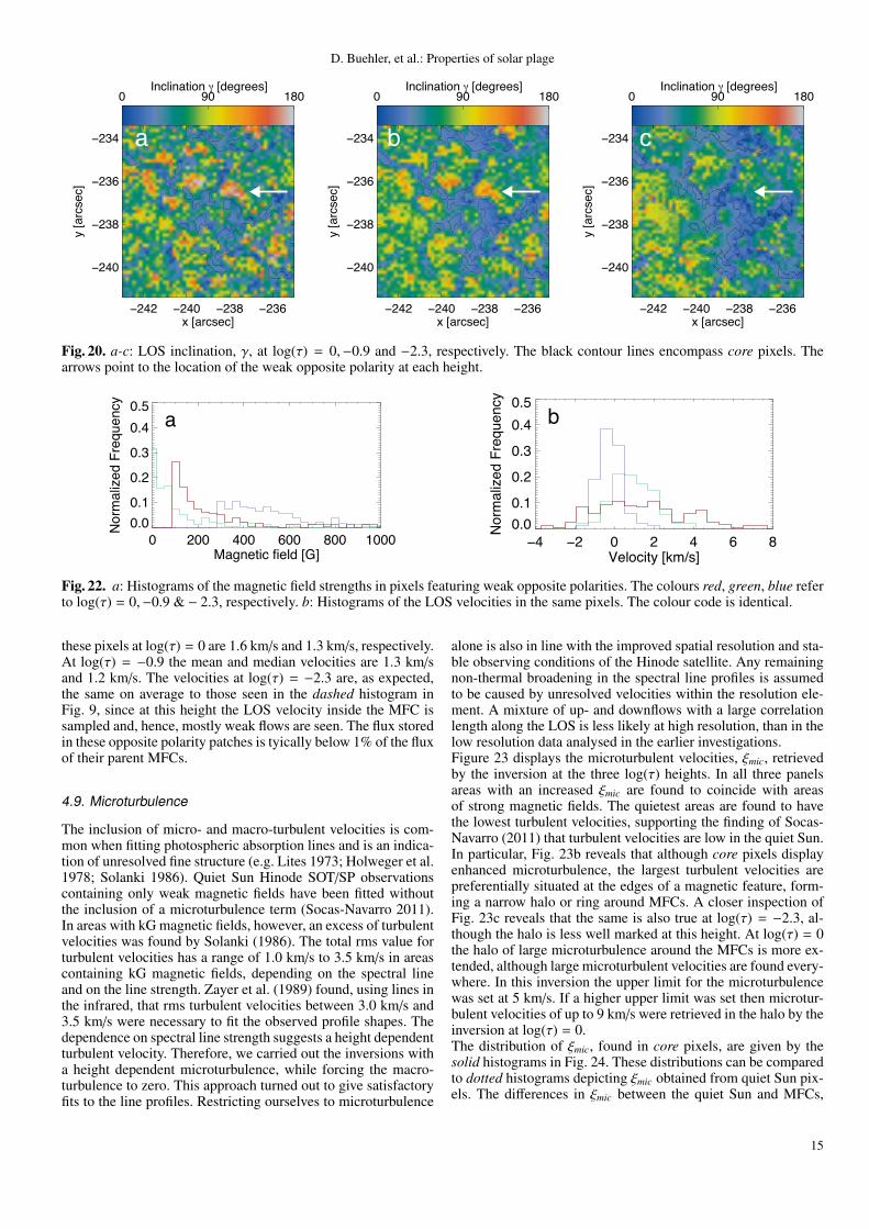
D. Buehler, et al.: Properties of solar plage
0 90 180
Inclination [degrees]
242 240 238 236x [arcsec]
240
238
236
234
y [a
rcse
c]
a
0 90 180
Inclination [degrees]
242 240 238 236x [arcsec]
240
238
236
234
y [a
rcse
c]
b
0 90 180
Inclination [degrees]
242 240 238 236x [arcsec]
240
238
236
234
y [a
rcse
c]
c
Fig. 20. a-c: LOS inclination, γ, at log(τ) = 0,−0.9 and −2.3, respectively. The black contour lines encompass core pixels. Thearrows point to the location of the weak opposite polarity at each height.
0 200 400 600 800 1000Magnetic field [G]
0.00.1
0.2
0.3
0.40.5
Nor
mal
ized
Fre
quen
cy
a
4 2 0 2 4 6 8Velocity [km/s]
0.00.1
0.2
0.3
0.40.5
Nor
mal
ized
Fre
quen
cyb
0 200 400 600 800 1000Magnetic field [G]
0.00.1
0.2
0.3
0.40.5
Nor
mal
ized
Fre
quen
cy
a
4 2 0 2 4 6 8Velocity [km/s]
0.00.1
0.2
0.3
0.40.5
Nor
mal
ized
Fre
quen
cy
b
Fig. 22. a: Histograms of the magnetic field strengths in pixels featuring weak opposite polarities. The colours red, green, blue referto log(τ) = 0,−0.9 & − 2.3, respectively. b: Histograms of the LOS velocities in the same pixels. The colour code is identical.
these pixels at log(τ) = 0 are 1.6 km/s and 1.3 km/s, respectively.At log(τ) = −0.9 the mean and median velocities are 1.3 km/sand 1.2 km/s. The velocities at log(τ) = −2.3 are, as expected,the same on average to those seen in the dashed histogram inFig. 9, since at this height the LOS velocity inside the MFC issampled and, hence, mostly weak flows are seen. The flux storedin these opposite polarity patches is tyically below 1% of the fluxof their parent MFCs.
4.9. Microturbulence
The inclusion of micro- and macro-turbulent velocities is com-mon when fitting photospheric absorption lines and is an indica-tion of unresolved fine structure (e.g. Lites 1973; Holweger et al.1978; Solanki 1986). Quiet Sun Hinode SOT/SP observationscontaining only weak magnetic fields have been fitted withoutthe inclusion of a microturbulence term (Socas-Navarro 2011).In areas with kG magnetic fields, however, an excess of turbulentvelocities was found by Solanki (1986). The total rms value forturbulent velocities has a range of 1.0 km/s to 3.5 km/s in areascontaining kG magnetic fields, depending on the spectral lineand on the line strength. Zayer et al. (1989) found, using lines inthe infrared, that rms turbulent velocities between 3.0 km/s and3.5 km/s were necessary to fit the observed profile shapes. Thedependence on spectral line strength suggests a height dependentturbulent velocity. Therefore, we carried out the inversions witha height dependent microturbulence, while forcing the macro-turbulence to zero. This approach turned out to give satisfactoryfits to the line profiles. Restricting ourselves to microturbulence
alone is also in line with the improved spatial resolution and sta-ble observing conditions of the Hinode satellite. Any remainingnon-thermal broadening in the spectral line profiles is assumedto be caused by unresolved velocities within the resolution ele-ment. A mixture of up- and downflows with a large correlationlength along the LOS is less likely at high resolution, than in thelow resolution data analysed in the earlier investigations.Figure 23 displays the microturbulent velocities, ξmic, retrievedby the inversion at the three log(τ) heights. In all three panelsareas with an increased ξmic are found to coincide with areasof strong magnetic fields. The quietest areas are found to havethe lowest turbulent velocities, supporting the finding of Socas-Navarro (2011) that turbulent velocities are low in the quiet Sun.In particular, Fig. 23b reveals that although core pixels displayenhanced microturbulence, the largest turbulent velocities arepreferentially situated at the edges of a magnetic feature, form-ing a narrow halo or ring around MFCs. A closer inspection ofFig. 23c reveals that the same is also true at log(τ) = −2.3, al-though the halo is less well marked at this height. At log(τ) = 0the halo of large microturbulence around the MFCs is more ex-tended, although large microturbulent velocities are found every-where. In this inversion the upper limit for the microturbulencewas set at 5 km/s. If a higher upper limit was set then microtur-bulent velocities of up to 9 km/s were retrieved in the halo by theinversion at log(τ) = 0.The distribution of ξmic, found in core pixels, are given by thesolid histograms in Fig. 24. These distributions can be comparedto dotted histograms depicting ξmic obtained from quiet Sun pix-els. The differences in ξmic between the quiet Sun and MFCs,
15

D. Buehler, et al.: Properties of solar plage
0 1 2 3 4 5
Microturbulence [km/s]
242 240 238 236x [arcsec]
240
238
236
234
y [a
rcse
c]
a
0 1 2 3 4
Microturbulence [km/s]
242 240 238 236x [arcsec]
240
238
236
234
y [a
rcse
c]
b
0.0 0.5 1.0 1.5 2.0 2.5
Microturbulence [km/s]
242 240 238 236x [arcsec]
240
238
236
234
y [a
rcse
c]
c
Fig. 23. a-c: Microturbulent velocities retrieved by the inversion at log(τ) = 0,−0.9 and −2.3 from left to right. Note the differentcolour scale for each frame. The black contour encompasses core pixels in all images. The dotted lines (in panel c) display canopypixels.
5000 5500 6000 6500 7000Temperaturelog( ) = 0 [K]
0.000.050.100.150.200.250.300.35
Nor
mal
ised
Fre
quen
cy5000 5500 6000 6500 7000
Temperaturelog( ) = 0 [K]
0.000.050.100.150.200.250.300.35
Nor
mal
ised
Fre
quen
cy
a
4500 5000 5500 6000 6500Temperaturelog( ) = 0.9 [K]
0.000.050.100.150.200.250.300.35
Nor
mal
ised
Fre
quen
cy
b
4000 4500 5000 5500 6000Temperaturelog( ) = 2.3 [K]
0.000.050.100.150.200.250.300.35
Nor
mal
ised
Fre
quen
cy
c
0 1 2 3 4 5Microturbulencelog( ) = 0 [km/s]
0.0
0.1
0.2
0.3
0.4
Nor
mal
ized
Fre
quen
cy
a
0 1 2 3 4 5Microturbulencelog( ) = 0.9 [km/s]
0.0
0.1
0.2
0.3
0.4
Nor
mal
ized
Fre
quen
cy
b
0 1 2 3 4 5Microturbulencelog( ) = 2.3 [km/s]
0.0
0.1
0.2
0.3
0.4
Nor
mal
ized
Fre
quen
cy
c
5000 5500 6000 6500 7000Temperaturelog( ) = 0 [K]
0.000.050.100.150.200.250.300.35
Nor
mal
ised
Fre
quen
cy
5000 5500 6000 6500 7000Temperaturelog( ) = 0 [K]
0.000.050.100.150.200.250.300.35
Nor
mal
ised
Fre
quen
cy
a
4500 5000 5500 6000 6500Temperaturelog( ) = 0.9 [K]
0.000.050.100.150.200.250.300.35
Nor
mal
ised
Fre
quen
cy
b
4000 4500 5000 5500 6000Temperaturelog( ) = 2.3 [K]
0.000.050.100.150.200.250.300.35
Nor
mal
ised
Fre
quen
cy
c
0 1 2 3 4 5Microturbulencelog( ) = 0 [km/s]
0.0
0.1
0.2
0.3
0.4
Nor
mal
ized
Fre
quen
cy
a
0 1 2 3 4 5Microturbulencelog( ) = 0.9 [km/s]
0.0
0.1
0.2
0.3
0.4
Nor
mal
ized
Fre
quen
cy
b
0 1 2 3 4 5Microturbulencelog( ) = 2.3 [km/s]
0.0
0.1
0.2
0.3
0.4
Nor
mal
ized
Fre
quen
cy
c
Fig. 24. Histograms of microturbulent velocities in core pixels, solid and the quiet Sun, dotted, at log(τ) = 0, a, at log(τ) = −0.9,b, and at log(τ) = −2.3, c. The dashed histogram in panel, c at log(τ) = −2.3, represents the microturbulent velocities of canopypixels.
0 1 2 3 4 5Microturbulence [km/s]
0.0
0.1
0.2
0.3
Nor
mal
ized
Fre
quen
cy
Fig. 25. Histograms of microturbulent velocities in pixels imme-diately surrounding core pixels, same as Fig. 11, at log(τ) = 0 inred and log(τ) = −0.9 in green. The dotted histograms show themicroturbulent velocities in the quiet Sun for the same layers.
suggested in Fig. 23, are confirmed by Fig. 24. At log(τ) = 0ξmic in the quiet Sun is on average slightly larger, with a mean
ξmic of 3.1 km/s, than in MFCs, which have an average velocityof 2.8 km/s. In higher layers the micro- turbulence in MFCs issignificantly larger than in the quiet Sun. Within the MFCs theaverage ξmic are 1.9 km/s and 1.3 km/s at log(τ) = −0.9 andlog(τ) = −2.3, whilst in the quiet Sun the average ξmic values are0.8 km/s and 0.4 km/s in the two layers, respectively. Note thatthe canopy pixels require a similar microturbulence as the corepixels at the same optical depth. Fig. 24 also reveals that in theupper two layers there are many pixels in the quiet Sun whichrequire no microturbulent broadening at all.The microturbulent velocities found in pixels, which are imme-diately adjacent to core pixels are displayed in Fig. 25. The pix-els used in this figure are identical to the ones used in Fig. 11,and are, therefore, the pixels featuring the highest LOS down-flow velocities. Again, only the microturbulence in the lower twolog(τ) layers are shown in Fig. 25 (due to the overlying canopyat log(τ) = −2.3). The average and median microturbulent ve-locities are 4.4 km/s and 5.0 km/s at log(τ) = 0 and 2.2 km/s and2.3 km/s at log(τ) = −0.9. These values are higher than those in
16

D. Buehler, et al.: Properties of solar plage
the quiet Sun and also than those found within the core pixels,demonstrating that the highest microturbulence is located at theedges of MFCs. Both the average and median values of ξmic atlog(τ) = 0 in the surrounding, downflowing pixels are likely tobe lower limits due to the upper bound of 5 km/s set on the mi-croturbulence in the inversion.The microturbulence retrieved by the inversion could, but doesnot necessarily imply the existence of turbulence or unresolvedconvective processes taking place within the magnetic features.It may point to unresolved waves in the MFC (e.g. surface wavescould account for the higher ξmic near the boundaries of theMFCs), or it may be due to unresolved horizontal velocity gradi-ents strongest at the boundaries. Another possibility may be, atleast in part, a signal of magnetic reconnection between the op-posite polarity fields found in this study (see Sect. 4.9). Althoughit cannot be completely ruled out that inaccuracies in the damp-ing constants of Fe I 6301.5 Å and 6302.5 Å (Anstee & O’Mara1995; Barklem & O’Mara 1997; Barklem et al. 1998) may con-tribute to the deduced ξmic, such inaccuracies are unable to ex-plain the excess in ξmic in the magnetic features, since the spec-tral lines are significantly weakened there, so that damping be-comes less important.
5. Discussion
In the preceding sections we sought to ascertain some of thecharacteristic properties of the magnetic field in solar plage.Stokes I, Q, U and V profiles of AR 10953 observed by theSOT/SP aboard Hinode were analysed using the SPINORinversion code (Frutiger et al. 2000), extended by van Noort(2012), to perform a spatially coupled 2D inversion, whichremoves the influence of the instrument’s PSF in parallel withinverting the data.The inversion was able to retrieve and reproduce many of thepreviously deduced characteristic properties of magnetic fluxconcentrations (MFCs) in plage regions. The typical magneticfield strength of MFCs was found to be in the kG range andtook on an average value of 1520 G at log(τ) = −0.9, where the6302 Å line pair is most sensitive to the magnetic field. Similarphotospheric magnetic field values were found previously byWiehr (e.g. 1978); Zayer et al. (e.g. 1990); Keller et al. (e.g.1990); Ruedi et al. (e.g. 1992); Rabin (e.g. 1992); Lin (e.g.1995); Martınez Pillet et al. (e.g. 1997). These values are,however, somewhat larger than those found using the Fe I5250.2/5247.1 Å line pair (e.g. Stenflo & Harvey 1985), whichis likely related to differences in the heights of formation of thetwo line pairs. Since no magnetic filling factor is introduced theobtained B values are lower limits to the true field strengths.The magnetic field is found to drop more slowly with heightwhen compared to a thin-tube (zeroth order) model. This lack ofagreement stems from a lack of flux conservation with height,by as much as 20%, that primarily affects the upper log(τ) nodein the inversion. If this increase in magnetic flux is compensatedthen the stratification of the strongest magnetic fields withstrengths higher than 2000 G, found at the centres of MFCs, doagree with the thin flux-tube model. When only the lower twolog(τ) layers are considered the model and the inversion alsoagree well. For magnetic fields < 2000 G at log(τ) = 0 othereffects start to play a role.The expansion of five isolated MFCs was compared to theideal expansion of two 0th order thin flux tube models. Theexpansion of the selected MFCs and the models agreed well,supporting previous results reported by Pietarila et al. (2010).
At the highest inverted layers the field did expand somewhatless rapidly than in the model, however, probably due tothe interactions (merging) with other magnetic features. Theinversion demonstrates that the majority of MFCs in the strongplage investigated here merge with neighbouring MFCs alreadyin the middle photosphere. Above the merging height B dropsmore slowly or not at all and the field also does not expandvery much (Pneuman et al. 1986; Steiner et al. 1986). The factthat a zeroth order flux tube is too simple to describe a MFC(Yelles Chaouche et al. 2009) and expands more rapidly thanmore realistic models that include curvature forces may alsocontribute.The LOS velocities obtained from the inversion show that thebulk of the magnetized gas in MFCs is essentially at rest andshows only weak downflows typically on the order of 200 m/s atlog(τ) = −0.9, which agrees with the results of Solanki (1986);Martınez Pillet et al. (1997). Some of the core and canopy pixelsshow upflows or downflows of up to 1 km/s, which were alsoobserved by Langangen et al. (2007). They are in most casesfound within the MFCs and could be the result of oscillationsor other transient events occurring within MFCs. The MFCs areeach surrounded by a ring of strong downflows, which can bereadily observed at the log(τ) = 0 and −0.9 nodes in Figs. 8 &10. These downflow rings were also seen to shift outwards inhigher log(τ) layers as the MFC expands. A downflow ring hasan average velocity of 2.4 km/s at log(τ) = 0, but parts of thering achieve supersonic velocities up to 10 km/s, correspondingto a Mach number of 1.25, in the same log(τ) layer. On average2.5% of a MFC’s ring contains downflows reaching supersonicvelocities. Some of these downflows appear to overlap with themagnetic field, which could be the signature of entrainment,or may be a result of insufficient spatial resolution to cleanlyresolve the magnetic boundary of MFCs. It is unlikely thatthey indicate convective collapse, since the Stokes V profilesof these pixels do not have the characteristic third lobe re-ported by Nagata et al. (2008). Downflows at the edges ofmagnetic features were previously found by Rouppe van derVoort et al. (2005) and Langangen et al. (2007). They are alsocompatible with the downflows inferred from the modelling ofStokes V asymmetries (Grossmann-Doerth et al. 1988; Solanki1989; Bunte et al. 1993). These downflows are strongest atlog(τ) = 0, gradually weaken higher up in the atmosphereand have completely disappeared at log(τ) = −2.3, suggestingthat they are associated with the granular convection pattern.However, downflows exceeding 6 km/s as well as supersonicvelocities are only found at the boundaries of MFCs and neverin the quiet Sun, indicating that the granular downflows arestrengthened by the presence of the MFC. We may be seeinga similar effect as at the edges of light-bridge granules, whichdisplay extremely strong downflows, probably because of acombination of radiative losses into the magnetic feature, whichleads to faster flows, and because the Wilson depression allowsus to see deeper layers with faster flows (Lagg et al. 2014). Thedownflows around MFCs also appear qualitatively similar tothe downflows observed around pores by Hirzberger (2003);Sankarasubramanian & Rimmele (2003) and Cho et al. (2010)and, therefore, might show a high temporal variation as well.Several MFCs also possess a plume-like downflow featurescharacterised by localised strong downflows traceable throughall log(τ) layers. These plumes become larger in size andsmaller in magnitude with height. They also trace the expansionof their MFC by shifting outwards with height. The origin ofthese plumes might be tied to a particular active granule in thevicinity, or may be caused by plasma pouring down from the
17

D. Buehler, et al.: Properties of solar plage
chromosphere. A reconnection event in the chromosphere mightalso give rise to such a structure, but the rapid increase of LOSvelocities with depth appears to be incompatible with such ascenario.Located within the downflow rings surrounding the MFCs, wefound small magnetic patches bearing the opposite polarity tothe main MFC to which they adjoin. These opposite polaritypatches are only visible in the lower two log(τ) nodes, asshown in Fig. 20, supporting the notion that they are intimatelyconnected to the downflows in which they are immersed. MHDsimulations carried out by Steiner et al. (1998) and Vogler et al.(2005) predict such patches in the vicinity of strong magneticfield concentrations, (see Fig. 5 in Vogler et al. 2005). Indirectevidence was also found in a network patch by Zayer et al.(1989), although the exact spatial proximity to the MFC couldnot be established in that publication due to the low spatialresolution. However, the reversal of the Stokes V amplitude inthe wings of the 630 nm line pair is only seen in the deconvolvedprofiles produced by the inversion, where the Stokes V spectrumdisplays three lobes. An additional complication is the maskingof these magnetic fields by the canopy of the main MFC.The canopy has a typical field strength of 300 G or higher atlocations overlying such weak opposite polarity fields. Thecanopy thus produces a strong signal in Stokes Q, U and V ,whereas the field strengths of the opposite polarity patches atlog(τ) = 0 are typically well below canopy values. This alsoprevents the selection of these patches via a typical amplitudethreshold in the Stokes profile, so that we cannot completelyrule out that even those opposite polarity patches with B¿100 Gare an artifact of the inversion. The opposite polarities typicallycarry less than 1% of the flux present in their parent MFCs.Further observations performed with a higher spatial resolutionare necessary to ascertain the existence of these small oppositepolarity patches. Such observations would be particularly usefulin the 1.56 µm lines, due to their large Zeeman sensitivity andlow formation height. The 1.56 µm data analysed by Zayer et al.(1989), although of low spatial resolution, provide some supportfor our results. The close coexistence of such opposite polaritiesmight give rise to current sheets and could lead to reconnectionevents.We have introduced a novel method for the resolution of the180◦ azimuth ambiguity applicable to largely unipolar regions.It makes use of the basic thin flux-tube structure of MFCs andassumes that the divergence of the magnetic field tends towardszero. With this method we find that the core pixels of MFCshave typical inclinations, relative to local solar coordinates,between 10◦ and 15◦ in all three log(τ) nodes of the inversion,which agrees well with earlier inclination results found byTopka et al. (1992); Bernasconi et al. (1995) and MartınezPillet et al. (1997). The distribution of the azimuths shows apreference for the eastern direction, which can be attributed to aLOS effect. MFCs located closest to the disc centre in the fieldof view showed the most homogeneous azimuth distribution,which supports the conclusion of Martınez Pillet et al. (1997)that in general MFCs have no preferred orientation. MFCs closeto the sunspot did, however, display azimuth distributions thatwere either predominantly directed towards or away from thespot depending on their polarity. The canopies of these MFCswere also irregular and elongated. This demonstrates that anearby sunspot has a direct impact on the properties of MFCseven in the middle photosphere.The inversion allowed us to clearly differentiate betweenmagnetic fields which form magnetic canopies from thosewhich form the core or root of a MFC. A separate canopy
could be identified for all MFCs as well as for the pores andsunspot. The canopies were found to harbour weaker, morehorizontal magnetic fields, with inclinations as high as Γ = 80◦.The typical LOS velocities in the canopies are identical to theLOS velocities found at the core of a MFC. Many magneticcanopies were found to lie above essentially field free regions.The canopies found here agree with the model proposed byGrossmann-Doerth et al. (1988) for the production of the StokesV area asymmetry and the observational results presented byRezaei et al. (2007); Narayan & Scharmer (2010) and MartınezGonzalez et al. (2012). All magnetic features were observed toexpand with height and many isolated MFCs merged to formcomparatively large expanses of magnetic field at log(τ) = −2.3.We therefore expect that at least some of the magnetic featuresdisplay a similarity to the wine-glass model described by Bunteet al. (1993).The average temperature stratification within MFCs mostclosely followed the empirical plage flux-tube model of Solanki& Brigljevic (1992). Temperatures were hotter by 300 K withinthe MFCs when compared to the quiet Sun in the upper twolog(τ) layers. However, a closer inspection of MFCs revealedthat the temperature is not homogeneous in any log(τ) acrossa MFC. The highest temperatures in a MFC are typicallypositioned at its edges and concentrated into isolated points atlog(τ) = 0. Often supersonic downflows were located in thevicinity of these temperature enhancements. This raises thepossibility that the two might be connected, since the supersonicflows likely create a shockfront below the log(τ) = 0 layer.However, there were also cases of temperature enhancementswithout a nearby supersonic velocity. It is likely that a clearpicture of the effect of these supersonic downflows upon anMFC can only be determined together with an analysis of a timeseries of data.The inversion procedure included a depth-dependent mi-croturbulent velocity, with the macroturbulence set to zero.Particularly high values of the microturbulence, partly inexcess of 5 km/s at log(τ) = 0, were found at the edges ofthe magnetic features. The typical microturbulent velocities inMFCs obtained by the inversion has an average value of 2.8km/s at log(τ) = 0 and becomes weaker with height. Suchvalues are on a par with the broadenings presented by Solanki(1986) and Zayer et al. (1989). This suggests the presence ofstrong unresolved velocities around the MFCs. Also, althoughits amplitude decreases rapidly with height, ξmic is at leasta factor of 2 larger in the MFC than in the quiet Sun in theupper two log(τ) layers. These large microturbulence valuesmay be telling us that the strong downflows at the edges ofthe MFCs are associated with vigorous turbulent motions, or itmay be a signature of waves travelling along the MFC. Finally,the microturbulence returned by the inversion code may besignalling strong horizontal velocity gradients, e.g. across theboundary of MFCs. A possible geometry for such gradients is astrong downflow outside and a weak one inside.
6. Conclusion
In this investigation we have been able to confirm many previ-ously obtained properties associated with magnetic fields, whichform solar plage. At the same time, we have also uncovered newfeatures associated with kG magnetic fields. KiloGauss fieldsin plage are strong, vertical (10◦ − 15◦) magnetic fields on theorder of 1.5 kG, which expand with height similar to a thinflux-tube forming extensive canopies as low as the upper photo-
18

D. Buehler, et al.: Properties of solar plage
sphere. These fields are further characterised by being on aver-age 300 K hotter than their surroundings in the middle and upperphotosphere, in agreement with empirical flux-tube models, andcontain weak, on average 200 m/s, plasma flows within them.This investigation has also discovered several new properties ofthese fields. Each magnetic flux concentration is surrounded bya ring containing strong downflows, on average 2.4 km/s in thelower photosphere. A typical ring shifts outward with height asthe field expands and parts of it can attain supersonic veloci-ties in the lower photosphere. Co-spatial with these rings wefound enhanced microturbulent velocities decreasing with heightas well as magnetic patches situated beneath the canopy with apolarity opposite to the main plage-forming fields. The plasmatemperature of the MFCs was not uniform across their crosssections, displaying instead temperature enhancements at theiredges. Magnetic field concentrations located close to larger fea-tures such as pores or a sunspot displayed an asymmetric canopyand more inclined magnetic fields.
Acknowledgements. Hinode is a Japanese mission developed and launched byISAS/JAXA, with NAOJ as domestic partner and NASA and STFC (UK) asinternational partners. It is operated by these agencies in co-operation withESA and NSC (Norway). This work has been partially supported by the BK21plus program through the National Research Foundation (NRF) funded by theMinistry of Education of Korea. D.B. acknowledges a PhD fellowship of theInternational Max Planck Research School on Physical Processes in the SolarSystem and Beyond (IMPRS).
ReferencesAnstee, S. D. & O’Mara, B. J. 1995, MNRAS, 276, 859Babcock, H. W. & Babcock, H. D. 1955, ApJ, 121, 349Barklem, P. S. & O’Mara, B. J. 1997, MNRAS, 290, 102Barklem, P. S., O’Mara, B. J., & Ross, J. E. 1998, MNRAS, 296, 1057Barthol, P., Gandorfer, A., Solanki, S. K., et al. 2011, Sol. Phys., 268, 1Berger, T. E., Rouppe van der Voort, L. H. M., Lofdahl, M. G., et al. 2004, A&A,
428, 613Bernasconi, P. N., Keller, C. U., Povel, H. P., & Stenflo, J. O. 1995, A&A, 302,
533Briand, C. & Solanki, S. K. 1998, A&A, 330, 1160Bruls, J. H. M. J. & Solanki, S. K. 1995, A&A, 293, 240Bunte, M., Solanki, S. K., & Steiner, O. 1993, A&A, 268, 736Cho, K.-S., Bong, S.-C., Chae, J., Kim, Y.-H., & Park, Y.-D. 2010, ApJ, 723, 440Danilovic, S., Gandorfer, A., Lagg, A., et al. 2008, A&A, 484, L17Danilovic, S., Schussler, M., & Solanki, S. K. 2010, A&A, 509, A76Defouw, R. J. 1976, ApJ, 209, 266Deinzer, W., Hensler, G., Schussler, M., & Weisshaar, E. 1984, A&A, 139, 435Elmore, D. F., Lites, B. W., Tomczyk, S., et al. 1992, in Society of Photo-Optical
Instrumentation Engineers (SPIE) Conference Series, Vol. 1746, PolarizationAnalysis and Measurement, ed. D. H. Goldstein & R. A. Chipman, 22–33
Frazier, E. N. & Stenflo, J. O. 1972, Sol. Phys., 27, 330Frutiger, C., Solanki, S. K., Fligge, M., & Bruls, J. H. M. J. 2000, A&A, 358,
1109Giovanelli, R. G. 1982, Sol. Phys., 80, 21Grossmann-Doerth, U., Schussler, M., & Solanki, S. K. 1988, A&A, 206, L37Grossmann-Doerth, U., Schussler, M., & Steiner, O. 1998, A&A, 337, 928Hale, G. E. 1908, ApJ, 28, 315Hirzberger, J. 2003, A&A, 405, 331Holweger, H., Gehlsen, M., & Ruland, F. 1978, A&A, 70, 537Howard, R. & Stenflo, J. O. 1972, Sol. Phys., 22, 402Ichimoto, K., Lites, B., Elmore, D., et al. 2008, Sol. Phys., 249, 233Ishikawa, R. & Tsuneta, S. 2009, A&A, 495, 607Ishikawa, R., Tsuneta, S., Ichimoto, K., et al. 2008, A&A, 481, L25Keller, C. U., Stenflo, J. O., Solanki, S. K., Tarbell, T. D., & Title, A. M. 1990,
A&A, 236, 250Kobel, P., Solanki, S. K., & Borrero, J. M. 2011, A&A, 531, A112Kobel, P., Solanki, S. K., & Borrero, J. M. 2012, A&A, 542, A96Kosugi, T., Matsuzaki, K., Sakao, T., et al. 2007, Sol. Phys., 243, 3Kuckein, C., Martınez Pillet, V., & Centeno, R. 2012, A&A, 539, A131Lagg, A., Solanki, S. K., Riethmuller, T. L., et al. 2010, ApJ, 723, L164Lagg, A., Solanki, S. K., van Noort, M., & Danilovic, S. 2014, A&A, 568, A60Langangen, Ø., Carlsson, M., Rouppe van der Voort, L., & Stein, R. F. 2007,
ApJ, 655, 615
Lawrence, J. K., Topka, K. P., & Jones, H. P. 1993, J. Geophys. Res., 98, 18911Leka, K. D., Barnes, G., Crouch, A. D., et al. 2009, Sol. Phys., 260, 83Lin, H. 1995, ApJ, 446, 421Lites, B. W. 1973, Sol. Phys., 32, 283Lites, B. W. & Ichimoto, K. 2013, Sol. Phys., 283, 601Martınez Gonzalez, M. J., Bellot Rubio, L. R., Solanki, S. K., et al. 2012, ApJ,
758, L40Martınez Pillet, V., Del Toro Iniesta, J. C., Alvarez-Herrero, A., et al. 2011,
Sol. Phys., 268, 57Martınez Pillet, V., Lites, B. W., & Skumanich, A. 1997, ApJ, 474, 810Metcalf, T. R., Leka, K. D., Barnes, G., et al. 2006, Sol. Phys., 237, 267Morinaga, S., Sakurai, T., Ichimoto, K., et al. 2008, A&A, 481, L29Nagata, S., Tsuneta, S., Suematsu, Y., et al. 2008, ApJ, 677, L145Narayan, G. & Scharmer, G. B. 2010, A&A, 524, A3Okamoto, T. J., Tsuneta, S., Lites, B. W., et al. 2008, ApJ, 673, L215Okamoto, T. J., Tsuneta, S., Lites, B. W., et al. 2009, ApJ, 697, 913Osherovich, V. A., Chapman, G. A., & Fla, T. 1983, ApJ, 268, 412Parker, E. N. 1978, ApJ, 221, 368Pietarila, A., Cameron, R., & Solanki, S. K. 2010, A&A, 518, A50Pneuman, G. W., Solanki, S. K., & Stenflo, J. O. 1986, A&A, 154, 231Rabin, D. 1992, ApJ, 391, 832Requerey, I. S., Del Toro Iniesta, J. C., Bellot Rubio, L. R., et al. 2014, ApJ, 789,
6Rezaei, R., Steiner, O., Wedemeyer-Bohm, S., et al. 2007, A&A, 476, L33Riethmuller, T. L., Solanki, S. K., van Noort, M., & Tiwari, S. K. 2013, A&A,
554, A53Rouppe van der Voort, L. H. M., Hansteen, V. H., Carlsson, M., et al. 2005,
A&A, 435, 327Ruedi, I., Solanki, S. K., Livingston, W., & Stenflo, J. O. 1992, A&A, 263, 323Sankarasubramanian, K. & Rimmele, T. 2003, ApJ, 598, 689Sasso, C., Lagg, A., & Solanki, S. K. 2011, A&A, 526, A42Scharmer, G. B., Bjelksjo, K., Korhonen, T. K., Lindberg, B., & Petterson,
B. 2003, in Society of Photo-Optical Instrumentation Engineers (SPIE)Conference Series, Vol. 4853, Innovative Telescopes and Instrumentation forSolar Astrophysics, ed. S. L. Keil & S. V. Avakyan, 341–350
Schussler, M. 1986, in Small Scale Magnetic Flux Concentrations in the SolarPhotosphere, ed. W. Deinzer, M. Knolker, & H. H. Voigt, 103
Shimizu, T., Nagata, S., Tsuneta, S., et al. 2008, Sol. Phys., 249, 221Socas-Navarro, H. 2011, A&A, 529, A37Socas-Navarro, H. & Manso Sainz, R. 2005, ApJ, 620, L71Solanki, S. K. 1986, A&A, 168, 311Solanki, S. K. 1989, A&A, 224, 225Solanki, S. K. 1993, Space Sci. Rev., 63, 1Solanki, S. K., Barthol, P., Danilovic, S., et al. 2010, ApJ, 723, L127Solanki, S. K. & Brigljevic, V. 1992, A&A, 262, L29Solanki, S. K., Finsterle, W., & Ruedi, I. 1996a, Sol. Phys., 164, 253Solanki, S. K., Finsterle, W., Ruedi, I., & Livingston, W. 1999, A&A, 347, L27Solanki, S. K., Keller, C., & Stenflo, J. O. 1987, A&A, 188, 183Solanki, S. K., Montavon, C. A. P., & Livingston, W. 1994, A&A, 283, 221Solanki, S. K., Ruedi, I., & Livingston, W. 1992, A&A, 263, 339Solanki, S. K. & Stenflo, J. O. 1984, A&A, 140, 185Solanki, S. K., Zufferey, D., Lin, H., Ruedi, I., & Kuhn, J. R. 1996b, A&A, 310,
L33Spruit, H. C. 1976, Sol. Phys., 50, 269Spruit, H. C. 1979, Sol. Phys., 61, 363Steiner, O., Grossmann-Doerth, U., Knolker, M., & Schussler, M. 1998, ApJ,
495, 468Steiner, O., Grossmann-Doerth, U., Schussler, M., & Knolker, M. 1996,
Sol. Phys., 164, 223Steiner, O., Pneuman, G. W., & Stenflo, J. O. 1986, A&A, 170, 126Stenflo, J. O. 1973, Sol. Phys., 32, 41Stenflo, J. O. 2010, A&A, 517, A37Stenflo, J. O. & Harvey, J. W. 1985, Sol. Phys., 95, 99Stenflo, J. O., Solanki, S., Harvey, J. W., & Brault, J. W. 1984, A&A, 131, 333Suematsu, Y., Tsuneta, S., Ichimoto, K., et al. 2008, Sol. Phys., 249, 197Title, A. M., Tarbell, T. D., Topka, K. P., et al. 1989, ApJ, 336, 475Tiwari, S. K., van Noort, M., Lagg, A., & Solanki, S. K. 2013, A&A, 557, A25Topka, K. P., Tarbell, T. D., & Title, A. M. 1992, ApJ, 396, 351Topka, K. P., Tarbell, T. D., & Title, A. M. 1997, ApJ, 484, 479Tsuneta, S., Ichimoto, K., Katsukawa, Y., et al. 2008, Sol. Phys., 249, 167Unno, W. 1956, PASJ, 8, 108van Noort, M. 2012, A&A, 548, A5van Noort, M., Lagg, A., Tiwari, S. K., & Solanki, S. K. 2013, A&A, 557, A24Venkatakrishnan, P. 1986, Nature, 322, 156Viticchie, B. & Sanchez Almeida, J. 2011, A&A, 530, A14Vogler, A., Shelyag, S., Schussler, M., et al. 2005, A&A, 429, 335Wiehr, E. 1978, A&A, 69, 279Xu, Z., Lagg, A., & Solanki, S. K. 2010, A&A, 520, A77
19

D. Buehler, et al.: Properties of solar plage
Yelles Chaouche, L., Solanki, S. K., & Schussler, M. 2009, A&A, 504, 595Zayer, I., Solanki, S. K., & Stenflo, J. O. 1989, A&A, 211, 463Zayer, I., Stenflo, J. O., Keller, C. U., & Solanki, S. K. 1990, A&A, 239, 356Zirin, H. & Popp, B. 1989, ApJ, 340, 571
20