pythagoras meets peano, courtesy of core logic

Pythagoras meets Peano,

courtesy of Core Logic

by

Neil Tennant∗

Department of PhilosophyThe Ohio State UniversityColumbus, Ohio 43210email [email protected]

December 13, 2015

Abstract

We present a completely formalized proof, down to the last primitivenumber-axiomatic and logical-inferential details, in Core Logic, of thestatement that no square of a natural number is twice any such square.

∗Please do not cite or circulate without the author’s permission.

1

1 The Challenge

In late August and early September 2015 there was a lively discussion,on the moderated email list [email protected], of Core Logic and the ques-tion whether the rule Ex Falso Quodlibet—conspicuously eschewed by CoreLogic—is indispensable for formalizing mathematical proofs.1 Harvey Fried-man issued as a challenge to the core logician the formalization of the ‘usualproofs’ of two well-known results in number theory.2 He asked, in particular,

What would a detailed analysis of Tennantism look like for, say,the usual proofs of

n2 = 2m2 has no solution in nonzero integers . . .

It seemed clear, reading between the lines, that Friedman was of the opin-ion that this could not be done. Here we address this particular challengeproblem—showing rigorously, in Core Logic, and from the Peano Axiomsfor arithmetic, that no square of a natural number is twice any such square(hence that the square root of 2 is irrational).

This, according to legend, is the discovery, made by some student orassociate of Pythagoras, that shook the Pythagorean dogma that the worldis made up out of whole numbers. One story has it that the proof led toits discover’s expulsion from the cult; another, that it led to his executionby the same. I trust, then, that merely formalizing the proof will not beconsidered any essential advance; for the metaphysical cat is already out ofthe mathematical bag.

The extension of this result to the nonzero integers is of course straight-forward, once one makes the move to the integers. The result is made allthe more difficult to obtain, however, by initially restricting oneself to thePeano Axioms, and not helping oneself axiomatically to the usual algebraiclaws (commutativity and associativity of addition and multiplication, forexample, as well as distributivity of multiplication over addition) that areusually laid down as axioms for the ring (or integral domain) of the integers.In Peano Arithmetic, such properties of addition and multiplication have tobe derived as theorems. This study ventures to present an absolutely formal,fully detailed proof, using only Core Logic, of the statement

∀x¬∃y(y 6=0 ∧ x.x=2.(y.y))

1Everything that the reader might need to know about Core Logic can be found in thethree publications Tennant [2012], Tennant [2015a] and Tennant [2015b].

2See http://www.cs.nyu.edu/pipermail/fom/2015-September/019105.html.

2

from Peano’s axioms for the natural numbers. Or, rather: it presents areplete set of chunks of core proof, that collectively make up a single formalproof of the target result. (See Theorem 1.) This is simply because I amworking within the confines of the A4 page. So I have had to break thedeductive reasoning down into manageable chunks for the reader. In orderto pull this off, there has been the occasional lapse into landscape mode.

The resounding theoretical answer to the aforementioned challenge prob-lem of Friedman is that Ex Falso Quodlibet is not needed for formalizingmathematical proofs. That much is established by metatheorems. All thatthis study contributes is a single, sustained and important example of howthis can be so. I do not usually take single-case inductions to be dispositivein foundational matters. But, in light of the metatheorems in the cited pub-lications on Core Logic, a core-logical formalization of the proof that

√2 is

irrational struck me as invitingly apt, illustrative, timely and worthwhile.It may be (for all I know) that this is the first time in the history of

humankind that such a proof has ever been presented. For, in any mathe-matics textbook that proves this result ‘rigorously’ (yet, strictly speaking,informally) the proof takes a scant half-page or so. Ironically, one is moremorally certain of the truth of the result on the basis of the informal proofthan one can be (unaided by any automated proof-checker) on the basis ofthe fully formalized proof. This is because the fully formalized proof is verylong, and it is psychically draining to check it for correctness. But suchepistemic ironies are beside the point here. It is enough to appreciate thatfulfilling the hand-waving promise by the formal logician that mathematicalproofs can be fully formalized is no easy task. What follows should go someway to convince the reader that this is so (both that it is possible and thatit is, nevertheless, no easy task). I am naturally relying on the orthodoxlogician—especially Friedman—who is keen to fault the core logician, tocheck the core proof offered here for formal correctness down to the verylast detail. This is no exercise in falsche Spitzfindigkeit. For it is undertakento meet Friedman’s challenge head-on, to show him (and anyone else whomay be interested) that Core Logic has what it takes to formalize informalexpert mathematical reasoning directly, naturally, and homologously.

2 Peano’s axioms for the natural numbers

The theory of natural numbers is expressed in the first-order language withidentity based on the name 0 (zero), the one-place function sign s (successor),and the two-place function signs + (plus) and . (times). For definiteness,

3

we take the theory to be axiomatized by the now famous axioms

∀x ¬ 0=sx∀x∀y(sx=sy → x=y)∀x x+0=x∀x∀y x+sy=s(x+y)∀x x.0=0∀x∀y x.sy=(x.y)+x

plus all (countably) infinitely many instances of the following axiom schemaof Mathematical Induction:

(P0 ∧ ∀x(Px→ Psx))→ ∀yPy

Whatever formula Px is used in order to obtain a substitution instance ofthis axiom schema is called the induced predicate for the instance in question.

Note that this choice of axioms means that certain number-theoreticstatements that the average mathematician would take as so obvious as notto stand in need of proof will actually have to be proved—indeed, in somecases, at quite considerable length. But that is just part of the bracingchallenge to be faced anyway.

3 Definitions of non-primitive notions

Definition 1. 1 =df s0

Definition 2. 2 =df ss0

Definition 3. m is less than n (in symbols: m<n)≡df ∃km+sk=n

Definition 4. m is less than or equal to n (in symbols: m≤n)≡df m<n ∨m=n

Definition 5.k divides n with remainder r (in symbols: k|n; r)≡df r < k ∧ ∃m n=(k.m+ r)

Definition 6.k divides n with no remainder (in symbols: k|n; 0, abbreviated further tok|n)≡df ∃m n=km

4

Definition 7.n is even (in symbols: En) ≡df 2|n. Equivalently, ss0|n. Equivalently,∃m n=ss0.m

Definition 8.n is odd (in symbols: On) ≡df 2|n; 1 Equivalently, ss0|n; s0. Equivalently,in light of Lemma 1: ∃m n=ss0.m+s0

In presenting our formal proofs below, we shall frequently resort to theserial forms of certain elimination rules. We do so in order to prevent side-ways spread; and also because the serial forms are likely to be more familiarto the reader than the parallelized forms. The occasional exception, whenparallelized forms are used, will be included in order to familiarize the readerwith how these forms of the rules are applied. We shall be at pains, however,to ensure that all the formal proofs we provide are in normal form. Also,they do not use Ex Falso Quodlibet. And sometimes they use the ‘liberal-ized’ rules of →I and ∨E of Core Logic. What these investigations reveal isjust how naturally the resources of Core Logic directly formalize the expertinformal reasoning employed in the proof that

√2 is not a ratio of whole

numbers.

4 On Formalizing Uses of the Principle of Mathe-matical Induction

We coin the description ‘incremental induction’ for the kind of MathematicalInduction whose axiom schema was stated above. Its being incremental isa matter of showing that the property in question is transmitted under thesuccessor operation. In proofs by induction, this corresponds to the familiarinductive step that appeals to the inductive hypothesis Pa to derive theconclusion Psa (for a suitably chosen individual parameter a).

Suppose that, when proceeding informally, one proves a lemma ∀yPy byusing an instance of (incremental) Mathematical Induction. That is, oneproves the ‘basis step’ P0; then one effects the ‘inductive step’ from theinductive hypothesis Pa to the conclusion Psa; and finally one invokes theinstance


of Mathematical Induction to conclude

∀yPy

5

The formalization of this stretch of reasoning would have the following over-all form:


∆ΠP0

(1)

Γ, Pa︸︷︷︸ΞPsa (1)

Pa→ Psa∀x(Px→ Psx)

P0 ∧ ∀x(Px→ Psx)(2)

∀yPy(2)

∀yPy

with the lemma ∀yPy as the overall conclusion. Here Π is the proof of the‘basis step’ P0 for the proof by induction; and Ξ is the proof of the ‘inductivestep’, using the inductive hypothesis Pa to deduce the conclusion Psa.

Two clarifying remarks are in order here.

Remark 1: One does not have to make use of the inductive hypothesis Pa;such use is permissible, not obligatory. The application of the rule of →I atthe step marked (1) ensures that the assumption Pa, if used, is discharged.But, to stress once again: it may turn out that there is no assumption ofthe form Pa to be discharged! The step of →I would still be in good order;the overall proof by induction would simply look like this:


∆ΠP0

ΓΞPsa


P0 ∧ ∀x(Px→ Psx)(2)

∀yPy(2)

∀yPy

Note, however, that if one is equipped with the subproofs

∆ΠP0

andΓΞPsa

as indicated, then the conclusion ∀yPy could be obtained as follows, using

6

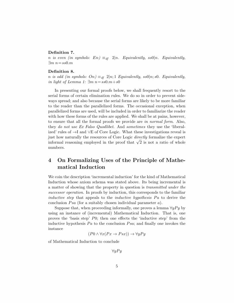
the premise ∀x(x=0 ∨ ∃y x=sy):

∀x(x=0 ∨ ∃y x=sy)

c=0 ∨ ∃y c=sy

∆ΠP0

(1)

c=0

Pc

(1)

∃y c=sy

ΓΞPsa

(2)

c=sa

Pc(2)

Pc(1)

Pc∀yPy

This extra premise is Lemma 8 below. It is the special axiom that, in Robin-son’s finitely axiomatized theory of arithmetic, replaces the Axiom Schemaof Mathematical Induction. As we shall presently see, there is a proof of∀x(x= 0 ∨ ∃y x= sy) in Peano Arithmetic, using an instance of the AxiomSchema of Mathematical Induction, that eschews any use of the inductivehypothesis.

Remark 2, complementary to Remark 1: One does not have to producePsa as the conclusion of the inductive step! It would suffice to simply reducethe inductive hypothesis Pa to absurdity. The step of →I would still be ingood order; the overall proof by induction would then look like this:


∆ΠP0

(1)

Γ, Pa︸︷︷︸Ξ⊥ (1)


P0 ∧ ∀x(Px→ Psx)(2)

∀yPy(2)

∀yPy

Note that the final step, marked (2), is an application of the parallelized ruleof →E, with a degenerate major subproof (which proves ∀yPy from ∀yPy).The major premise of that application of →E is the chosen instance of theaxiom schema of Mathematical Induction. The minor subproof for the stepof →E in question is the subproof ‘in the middle’, of P0 ∧ ∀x(Px → Psx).The two subproofs Π, Ξ can of course use, in addition, any of the Peanoaxioms, along with other suppositions. These respectively form the twosets ∆, Γ indicated in blue. When ∆, Γ contain only axioms, then (what

7

the mathematicians call the lemma) ∀yPy is (what logicians would call) atheorem of Peano arithmetic. Otherwise, ∀yPy is a result following, withinthe theory of arithmetic, conditionally upon the extra suppositions in ∆, Γthat are not axioms.

Suppose now that one subsequently appeals to the mathematicians’ lemma∀yPy as a premise in some further proof (call it Σ) of a conclusion θ onwhich the mathematicians are willing to bestow the honorific label ‘theo-rem’ (of Peano arithmetic). Then in the formalization of this overall stretchof reasoning there is no call for a so-called ‘cut’ with the lemma in question(∀yPy) as the cut sentence. This is because the overall formal proof ofthe mathematical theorem θ in such circumstances will be able to take thefollowing shape:


∆ΠP0

(1)



P0 ∧ ∀x(Px→ Psx)

(i)

Ω, ∀yPy︸︷︷︸Σθ(i)

θ

Here Π and Ξ are as before; but now the major subproof for the final stepof →E is one’s proof Σ of θ, which uses the lemma ∀yPy as a premise. Sothe final step is still an application of the parallelized rule of →E, but nowwith a non-degenerate major subproof, namely Σ. The major premise of thefinal step is still the chosen instance of the axiom schema of MathematicalInduction. The three subproofs Π, Ξ and Σ can of course use, in addition,any of the Peano axioms, along with other suppositions. These respectivelyform the three sets ∆, Γ and Ω indicated in blue. When ∆, Γ and Ω containonly axioms, then θ is a theorem of Peano arithmetic. Otherwise, θ is aresult following, within the theory of arithmetic, conditionally upon theextra suppositions in ∆, Γ and Ω that are not axioms.

In an effort to prevent sideways spread it would be quite in order to

8

suppress the major premise for →E on the left:

∆ΠP0

(1)




(i)

Ω, ∀yPy︸︷︷︸Σθ

(i)

θ

For it can be efectively determined what the induced predicate is, for suchan application of induction.

The Principle of Mathematical Induction can be parallelized even fur-ther, as follows:


∆ΠP0

(1)




Ω ,(i)

Pt1 , . . . ,(i)

Ptn︸︷︷︸Σθ

(i)

θ

since there will only over be finitely many appeals to the lemma ∀yPy thathas been established by induction. These appeals will involve singular termst1, . . . , tn (which may be, or contain, parameters). Indeed, the parallelizedrule just stated can be ‘inferentialized’ even further, and its major premisesuppressed, so as to become the Rule of Mathematical Induction

rmi∆ΠP0

(i)

Γ, Pa︸︷︷︸Ξ

⊥/Psa

Ω ,(i)

Pt1 , . . . ,(i)

Ptn︸︷︷︸Σθ

(i)

θ

Note how we have designated the conclusion of the proof Ξ of the inductivestep as ‘⊥/Psa’. This is pursuant to Remarks 1 and 2 above. In the fore-going statement of the rule rmi, it is to be understood that the proof Ξ ofthe inductive step satisfies exactly one of the following conditions:

9

1. Ξ has Pa as an undischarged assumption, and has ⊥ as its conclusion;

2. Ξ has Pa as an undischarged assumption, and has Psa as its conclu-sion;

3. Ξ does not have Pa as an undischarged assumption, and has Psa asits conclusion.

In each of the first two cases, the application of rmi discharges all assumption-occurrences of Pa in Ξ. In the third case, such discharge is not called for,since Pa is not used as an assumption.

Note that with applications of rmi each of Π, Ξ and Σ is a proof. Thisshould go without saying, since rules of inference enable one to form proofs,but only from (simpler) proofs. There is a special need here, however, tostress that the major subproof Σ has to be well formed. In particular, if anyof the terms t1, . . . , tn is (or contains) a parameter a, then a cannot occur insuch a way as to violate any of the parametric restrictions on applications,within Σ, of the two rules ∃E and ∀I, applications of which might well haveto involve a as a parameter. This places a limitation on the extent to whichone might be able to defer applications of rmi to points ‘lower down’ withina proof. They may instead have to be applied ‘higher up’, so as to dischargethose assumptions Pti that contain parameters that would otherwise, ifallowed to occur in those same assumptions undischarged, render illegitimatean application, within Σ, of either ∃E or ∀I.

As a special case (for n=1) we have

∆ΠP0

(i)


⊥/Psa(i)

Pt(i)

Pt

And as a further special case of that we have, with parameter b as one’schoice for the term t, the proof-schema

∆ΠP0

(i)


⊥/Psa(i)

Pb(i)

Pb

10

With b chosen so as to meet the requirements for ∀I, we can then obtain theusual conclusion ∀yPy of the proof by mathematical induction:

∆ΠP0

(i)


⊥/Psa(i)

Pb(i)

Pb∀yPy

If in fact one did this, and subsequently appealed to ∀yPy as a major premisefor ∀E in a proof of θ:

∀yPy

Ω ,(1)

Pt1 , . . . ,(1)

Ptn︸︷︷︸Σθ

(1)

θ

one would have a prime-facie violation of the requirement of normality forone’s overall proof of θ from ∆,Γ,Ω. But such an appearance of abnormalityis just that: a mere appearance. For one can always take for the genuinelyunderlying proof the reduct

∆ΠP0

(i)


⊥/Psa(i)

Pb(i)

Pb∀yPy

,

∀yPy

Ω ,(1)

Pt1 , . . . ,(1)

Ptn︸︷︷︸Σθ

(1)

θ

which is simply the form rmi (Rule of Mathematical Induction) stated above.As a convenient reminder:

rmi∆ΠP0

(i)


⊥/Psa

Ω ,(i)

Pt1 , . . . ,(i)

Ptn︸︷︷︸Σθ

(i)

θ

11

There is no blowup in length of proof, when taking the reduct in place of thetwo proofs between the square brackets. That much is absolutely obvious byinspection.

5 Results proved without using Mathematical In-duction

Because we are restricting our primitive means of mathematical expressionto the name 0 (zero), the one-place function sign s (successor), and thetwo-place function signs + (plus) and . (times), we have had to define cer-tain other expressions that mathematicians conveniently take as expressivelyprimitive. We saw this in §3.

Lemma 1. 1 < 2, i.e., s0 < ss0.

Proof.3

∀x∀y x+sy=s(x+y)

∀y s0+sy=s(s0+y)

s0+s0=s(s0+0)∀xx+0=xs0+0=s0

s0+s0=ss0∃k s0+sk=ss0i.e., s0 < ss0

Pause for a moment’s reflection . . . We have just taken five primitivesteps of inference to establish the trivial truth that 0 < 1. The alarmedreaction might be ‘To what dreadful lengths will we have to go in order toshow that no square of a natural is twice any such square’? The answer,reassuringly, is that the proof of the latter can be broken down into manage-able chunks, all of them formal proofs in Core Logic, using only the Peanoaxioms. The rest of this study shows how.

Lemma 2. 0 is not a successor; in symbols, expressed inferentially:

0=st⊥

3This proof is due to Ben Cleary.

12

Proof.∀x¬0=sx¬0=st 0=st

⊥

Trivially, also, we havest=0⊥

Lemma 3.st=sut = u

Proof.∀x∀y(sx=sy → x=y)

∀y(st=sy → t=y)

st=su→ t=u st=su(1)

t=u(1)

t=u

Note that the last step of this proof is an application of the parallelized rule→I, with a degenerate major subproof. We shall frequently use the rule ofinference stated in this lemma as a primitive rule, since it saves a great dealof sideways spread. Likewise with any other inferential rules that we haveestablished formally, such as those of Lemma 2.

Lemma 4.λ.λ 6=0

λ 6=0

Proof.

λ.λ 6=0

λ.λ=λ.λ(1)

λ=0

λ.λ=λ.0∀xx.0=0λ.0=0

λ.λ=0

⊥ (1)

λ 6=0

Lemma 5.λ=n.ρ λ 6=0

ρ 6=0

13

Proof.

λ 6=0

λ=n.ρ

n.ρ=n.ρ(1)

ρ=0

n.ρ=n.0∀xx.0=0n.0=0

n.ρ=0

λ=0

⊥ (1)

ρ 6=0

Lemma 6. From the assumption that a is even it follows that sa is odd

Proof.

∃ma=ss0.m

Lemma 1:s0<ss0

sa = sa(1)

a = ss0.b

sa = s(ss0.b)∀xx = x+0

ss0.b = ss0.b+0

sa = s(ss0.b+0)

∀x∀y x+sy = s(x+y)

∀y ss0.b+sy = s(ss0.b+y)

ss0.b+s0 = s(ss0.b+0)

sa=ss0.b+ s0

s0<ss0 ∧ sa=ss0.b+ s0ss0|sa; s0

(1)

ss0|sa; s0

Note that Lemma 1 is not a cut sentence here of the kind that would, uponaccumulation of proofs, produce an abnormal proof. Rather, the earlierproof of Lemma 1 could be inserted above its ‘premise occurrence’ in thelast proof just given, and the resulting proof would still be a proof in CoreLogic. We have broken the reasoning down into these last two chunks (proofof Lemma 1 followed by proof of Lemma 6) solely in order to avoid unman-ageable sideways spread on an A4 page. This is a theme that will be reprisedquite frequently below, and we shall not take the trouble to remark on itany further.

Lemma 7. ss0 = ss0.s0

14

Proof.

∀x∀y s(x+y)=x+sy

∀y s(0+y)=0+sy

s(0+s0)=0+ss0


∀y s(0+y)=0+sy

s(0+0)=0+s0∀x x+0=x

0+0=0

s0=0+s0

ss0=0 + ss0

∀x∀y x.sy=x.y+x

∀y ss0.sy=ss0.y+ss0

ss0.s0=ss0.0+ss0∀x x.0=xss0.0=0

ss0.s0=0+ss0

ss0=ss0.s0

6 Results proved using Mathematical Induction

For the formal proofs to follow, if we were to cite the actual instances tobe used of the axiom schema of Mathematical Induction, it would be pro-hibitively difficult to accommodate sideways spread on the page. We shalltherefore offer proofs in which Mathematical Induction takes the last-statedform of a rule of inference, namely rmi.

Lemma 8. Every number is either 0 or a successor; in symbols:

∀y(y=0 ∨ ∃x y=sx)

Proof.

0=00=0 ∨ ∃x 0=sx

(3)

a=0 ∨ ∃x a=sx

(2)

a=0sa=s0∃x sa=sx

(2)

∃x a=sx

(1)

a=sbsa=ssb∃x sa=sx

(1)

∃x sa=sx(2)

∃x sa=sxsa=0 ∨ ∃x sa=sx

(3)

c=0 ∨ ∃x c=sx(3)

c=0 ∨ ∃x c=sx∀y(y=0 ∨ ∃x y=sx)

The final step (of rmi) in this proof appears to involve an inductive stepthat actually uses the inductive hypothesis

a=0 ∨ ∃x a=sx

15

to derivesa=0 ∨ ∃x sa=sx.

There is, though, an even shorter proof by induction which does not use theinductive hypothesis at all:

0=00=0 ∨ ∃x 0=sx

sa=sa∃x sa=sx

sa=0 ∨ ∃x sa=sx(3)

c=0 ∨ ∃x c=sx(3)

c=0 ∨ ∃x c=sx∀y(y=0 ∨ ∃x y=sx)

Having established the ‘Q-axiom’ (Lemma 8), we can re-state it as anatomicized rule of inference, which we shall label QR (for ‘Q-Rule’):

QR

2 (i)

t = 0...

ψ/⊥

2 (i)

t = sa...

ψ/⊥(i)

ψ/⊥

where a is parametric

We shall now use the rule QR to prove the ‘zero-cancellation’ law.

Lemma 9.su.t=0t=0

Proof.

(1)

t=0

su.t=0(1)

t=sa

su.sa=0

∀x∀y x.sy=x.y+x

∀y su.sy=su.y+su

su.sa=su.a+su

su.a+su=0


∀y su.a+sy=s(su.a+y)

su.a+su=s(su.a+u)

s(su.a+u)=0

⊥(1) QR

t=0

Lemma 10.m<sam≤a

16

Proof. Unpacking the definitions of < and ≤, the rule to be derived amountsto

∃ym+sy=sa

∃z m+sz=a ∨m=a

and its derivation, using QR, is as follows:

∃ym+sy=sa

(1)

m+sb=sa(2)

b=0

m+s0=sa


∀ym+sy=s(m+y)

m+s0=s(m+0)

s(m+0)=sa∀xx+0=xm+0=m

sm=sa L3m=a

∃z m+sz=a ∨m=a

(1)

m+sb=sa(2)

b=sc

m+ssc=sa


∀ym+sy=s(m+y)

m+ssc=s(m+sc)

s(m+sc)=saL3

m+sc=a∃z m+sz=a

∃z m+sz=a ∨m=a(2) (QR)

∃z m+sz=a ∨m=a(1)

∃z m+sz=a ∨m=a

Corollary 1.m≤sa

m≤a ∨m=sa

Proof.

m≤sai.e., m<sa ∨m=sa

(1)

m<sa L10

m≤am≤a ∨m=sa

(1)

m=sam≤a ∨m=sa

(1)

m≤a ∨m=sa

Lemma 11. (b+b)+s0 = b+(b+s0)

Proof. The induced predicate is (x+x)+s0 = x+(x+s0). For the basis weneed to prove

(0+0)+s0 = 0+(0+s0)

The following formal proof does the job:

(0+0)+s0=(0+0)+s0


∀y (0+0)+sy=s((0+0)+y)

(0+0)+s0=s((0+0)+0)

(0+0)+s0=s((0+0)+0)∀xx+0=x

(0+0)+0=0+0

(0+0)+s0=s(0+0)∀xx+0=x0+0=0

(0+0)+s0=s(0+(0+0))


∀y 0+sy=s(0+y)

0+s(0+0)=s(0+(0+0))

(0+0)+s0=0+s(0+0)


∀y 0+sy=s(0+y)

0+s0=s(0+0)

(0+0)+s0 = 0+(0+s0)

17

For the inductive step we do not need to use the inductive hypothesis

(a+a)+s0 = a+(a+s0).

Instead, we prove(sa+sa)+s0 = sa+(sa+s0)

directly as follows.


∀y s(sa+a)+sy=s(s(sa+a)+y)

s(sa+a)+s0=s(s(sa+a)+0)


∀y sa+sy=s(sa+y)

sa+sa=s(sa+a)

(sa+sa)+s0=s(s(sa+a)+0)∀xx+0=x

s(sa+a)+0=s(sa+a)

(sa+sa)+s0=ss(sa+a)


∀y sa+sy=s(sa+y)

sa+sa=s(sa+a)

(sa+sa)+s0=s(sa+sa)


∀y sa+sy=s(sa+y)

sa+ssa=s(sa+sa)

(sa+sa)+s0=sa+ssa∀xx+0=xsa+0=sa

(sa+sa)+s0=sa+s(sa+0)


∀y sa+sy=s(sa+y)

sa+s0=s(sa+0)

(sa+sa)+s0 = sa+(sa+s0)

Lemma 12. b+s0=s0+b.

Proof. The induced predicate is x+s0 = s0+x. For the basis we need toprove

0+s0=s0+0



∀y 0+sy=s(0+y)

0+s0=s(0+0)∀xx+0=x

0+0=0

0+s0=s0∀xx+0=xs0+0=s0

0+s0=s0+0

For the inductive step we use the inductive hypothesis

a+s0=s0+a.

From it we provesa+s0=s0+sa

18

as follows.


∀y sa+sy=s(sa+y)

sa+s0=s(sa+0)∀xx+0=xsa+0=sa

sa+s0=ssa∀xx+0=xa+0=a

sa+s0=ss(a+0)


∀y a+sy=s(a+y)

a+s0=s(a+0)

sa+s0=s(a+s0)IH:

a+s0=s0+a

sa+s0=s(s0+a)


∀y s0+sy=s(s0+y)

s0+sa=s(s0+a)

sa+s0=s0+sa

Lemma 13. ∀x 0+x=x

Proof.

∀xx+0=x0+0=0


∀y 0+sy=s(0+y)

0+sa=s(0+a)(1)

0+a=a

0+sa=sa(1)

0+b=b(1)

0+b=b∀x 0+x=x

Lemma 14. ∀x 0+x=x+0

Proof.

0+0=0+0


∀y 0+sy=s(0+y)

0+sa=s(0+a)(1)

0+a=a+0

0+sa=s(a+0)∀xx+0=xa+0=a

0+sa=sa∀xx+0=xsa+0=sa

0+sa=sa+0(1)

0+b=b+0(1)

0+b=b+0∀x 0+x=x+0

19

Lemma 15. t.s0= t

Proof.∀x∀y x.sy=x.y+x

∀y t.sy= t.y+t

t.s0= t.0+t∀xx.0=0t.0=0

t.s0=0+tLemma 13:

0+t= t

t.s0= t

Lemma 16. 0.t=0

Proof.

∀xx.0=00.0=0

∀x∀y x.sy=x.y+x

∀y 0.sy=0.y+0

0.sa=0.a+0∀xx+0=x0.a+0=0.a

0.sa=0.a 0.a=0

0.sa=0(1)

0.t=0(1)

0.t=0

Lemma 17. s0.t= t

Proof.

∀xx.0=0s0.0=0

∀x∀y x.sy=x.y+x

∀y s0.sy=s0.y+s0

s0.sa=s0.a+s0(1)

s0.a=a

s0.sa=a+s0


∀y a+sy=s(a+y)

a+s0=s(a+0)

s0.sa=sa∀xx+0=xa+0=a

s0.sa=sa(1)

s0.t= t(1)

s0.t= t

The following result is called the ‘additive cancellation’ law. We shall in-novate by casting not only its statement, but also its inductive proof, in‘rule-inferential’ form.

20

Lemma 18.t+ k = u+ k

t = u

Proof. By induction, with the induced rule

t+n=u+nt=u

Because we are doing this inductive proof inferentially, the task for the basisis that of deriving the ‘basis rule’

t+0=u+0t=u

Moreover, the task for the inductive step is that of using the ‘inductivehypothesis’ rule

t+a=u+at=u

to derive the rulet+sa=u+sa

t=u

With that much by way of preparation we proceed to the ‘rule-inductive’proof itself.

The basis proof is as follows:

t+0=u+0∀xx+0=xt+0= t

t=u+0∀xx+0=xu+0=u

t=u

The proof of the inductive step (using the rule version of the InductiveHypothesis) is


∀y t+sy=s(t+y)

t+sa=s(t+a) t+sa=u+sa

s(t+a)=u+sa


∀y u+sy=s(u+y)

u+sa=s(u+a)

s(t+a)=s(u+a)L3

t+a=u+a IHt=u

21

Lemma 19. ∀x∀y x+sy=sx+y

Proof.


∀y a+sy=s(a+y)

a+s0=s(a+0)∀xx+0=xa+0=a

a+s0=sa∀xx+0=xsa+0=sa

a+s0=sa+0


∀y a+sy=s(a+y)

a+ssb=s(a+sb)(1)

a+sb=sa+b

a+ssb=s(sa+b)


∀y sa+sy=s(sa+y)

sa+sb=s(sa+b)

a+ssb=sa+sb(1)

a+sc=sa+c(1)

a+sc=sa+c∀y a+sy=sa+y

∀x∀y x+sy=sx+y

Lemma 20. ∀x∀y x+y=y+x

Proof.

Lemma 14:a+0=0+a


∀y a+sy=s(a+y)

a+sb=s(a+b)(1)

a+b=b+a

a+sb=s(b+a)


∀y b+sy=s(b+y)

b+sa=s(b+a)

a+sb=b+sa

Lemma 19:b+sa=sb+a

a+sb=sb+a(1)

a+c=c+a(1)

a+c=c+a∀y a+y=y+a

∀x∀y x+y=y+x

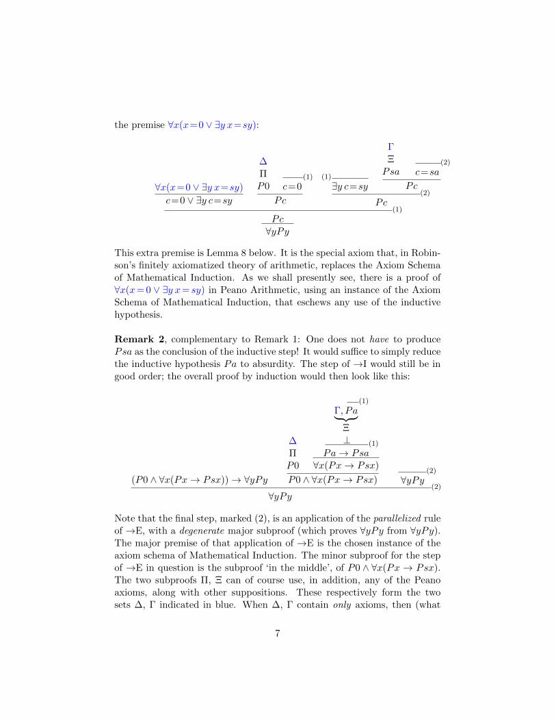
Corollary 2. t+(u+t) = (t+u)+t

Proof.Lemma 20:

t+(u+t)=(u+t)+tLemma 20:t+u=u+t

t+(u+t)=(t+u)+t

Lemma 21. t+(u+v) = (t+u)+v

22

Proof.

a+b=a+b∀xx+0=x

(a+b)+0=a+b

(a+b)+0=a+b∀xx+0=xb=b+0

(a+b)+0=a+(b+0)


∀y (a+ b)+sy=s((a+ b)+y)

(a+b)+sc=s((a+b)+c)(1)

(a+b)+c=a+(b+c)

a+(b+sc)=s(a+(b+c))


∀y a+sy=s(a+y)

a+s(b+c)=s(a+(b+c))

(a+b)+sc=a+s(b+c)


∀y b+sy=s(b+y)

b+sc=s(b+c)

(a+b)+sc=a+(b+sc)(1)

t+(u+v)=(t+u)+v

23

Lem

ma

22.st.u

=(t.u

)+u

Pro

of.

By

ind

uct

ion

,w

ith

the

ind

uce

dp

red

icat

esa.x

=a.x

+x

.T

he

bas

isp

roof

isas

foll

ows:

∀xx.0

=0

sa.0

=0

∀xx

+0

=x

0+

0=

0∀xx.0

=0

a.0

=0

a.0

+0

=0

sa.0

=a.0

+0

Th

ep

roof

ofth

ein

du

ctiv

est

epis

∀x∀y

x.sy=x.y+x

∀ysa

.sy=sa

.y+sa

)

sa.sc=sa

.c+sa

IH:

sa.c=a.c+c

sa.sc=(a.c+c)+sa

Lem

ma21:

(a.c+c)+sa

=a.c+(c+sa

)

sa.sc=a.c+(c+sa

)

∀x∀y

x+sy

=s(x+y)

∀yc+sy

=s(c+y)

c+sa

=s(c+a)

sa.sc=a.c+s(c+a)

Lem

ma20:

a+c=c+a

sa.sc=a.c+s(a+c)

∀x∀y

x+sy

=s(x+y)

∀ya.c+sy

=s(a.c+y)

a.c+s(a+c)=s(a.c+(a

+c))

sa.sc=s(a.c+(a

+c))

Lem

ma21:

a.c+(a

+c)=(a.c+a)+

c

sa.sc=s((a.c+a)+

c)

∀x∀y

x+sy

=s(x+y)

∀y(a.c+a)+

sy=s((a.c+a)+

y)

(a.c+a)+

sc=s((a.c+a)+

c)

sa.sc=(a.c+a)+

sc

∀x∀y

x.sy=x.y+x

∀ya.sy=a.y+a

a.sc=a.c+a

sa.sc=a.sc+sc

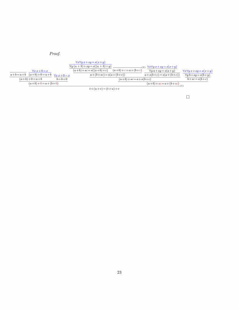
Lemma 23. t.u=u.t

Proof. By induction, with the induced predicate a.x== x.a. The basis proofis as follows:

∀xx.0=0a.0=0

Lemma 16 :0.a=0

a.0== 0.a

The proof of the inductive step is

∀x∀y x.sy=x.y+x

∀y a.sy=a.y+a

a.sb=a.b+a

Lemma 22 :sb.a=b.a+a

IH :a.b=b.a

sb.a=a.b+a

a.sb== sb.a

Lemma 24. t.(u+v)=(t.u)+(t.v)

Proof. By induction, with the induced predicate a.(b+x) = a.b+a.x. Thebasis proof is as follows:

a.b=a.b∀xx+0=xb+0=b

a.(b+0)=a.b∀xx+0=xa.b+0=a.b

a.(b+0)=a.b+0∀xx.0=0a.0=0

a.(b+0)=a.b+a.0


a.(b+sc)=a.(b+sc)


∀y b+sy=s(b+y)

b+sc=s(b+c)

a.(b+sc)=a.s(b+c)

∀x∀y x.sy=x.y+x

∀y a.sy=a.y+a

a.s(b+c)=a.(b+c)+a

a.(b+sc)=a.(b+c)+aIH:

a.(b+c)=a.b+a.c

a.(b+sc)=(a.b+a.c)+aLemma 21:

(a.b+a.c)+a=a.b+(a.c+a)

a.(b+sc)=a.b+(a.c+a)

∀x∀y x.sy=x.y+x

∀y a.sy=a.y+a

a.sc=a.c+a

a.(b+sc)=a.b+a.sc

Lemma 25. t.(u.v) = (t.u).v

25

Proof. By induction, with the induced predicate (a.b).x = a.(b.x). The basisproof is as follows:

∀xx.0=0(a.b).0=0

∀xx.0=0a.0=0

∀xx.0=0b.0=0

a.(b.0)=0

(a.b).0=a.(b.0)


∀x∀y x.sy=x.y+x

∀y (a.b).sy=(a.b).y+(a.b)

(a.b).sc=(a.b).c+ (a.b)

IH:(a.b).0=a.(b.0)

(a.b).sc=a.(b.c) + (a.b)Lemma 24:

a.(b.c+ b)=a.(b.c) + (a.b)

(a.b).sc=a.(b.c+ b)

∀x∀y x.sy=x.y+x

∀y b.sy=b.y+b

b.sc=b.c+ b

(a.b).sc=a.(b.sc)

Lemma 26. ss0.u = u+u

Proof. The induced predicate is ss0.x = x+x. For the basis we need toprove

ss0.0 = 0+0


∀xx.0=0ss0.0=0

∀xx+0=x0+0=0

ss0.0 = 0+0

For the inductive step we use the inductive hypothesis

ss0.a = a+a.

From it we provess0.sa = sa+sa

as follows.∀x∀y x.sy=x.y+x∀y ss0.sy=ss0.y+ss0ss0.sa=ss0.a+ss0

IH:ss0.a=a+a

ss0.sa=(a+a)+ss0

∀x∀y x+sy=s(x+y)∀y (a+a)+sy=s((a+a)+y)

(a+a)+ss0=s((a+a)+s0)

ss0.sa=s((a+a)+s0)Lemma 11:

(a+a)+s0=a+(a+s0)

ss0.sa=s(a+(a+s0))Lemma 12:a+s0=s0+a

ss0.sa=s(a+(s0+a))Corollary 2:

a+(s0+a)=(a+s0)+a

ss0.sa=s((a+s0)+a)

∀x∀y x+sy=s(x+y)∀y (a+s0)+sy=s((a+s0)+y)

(a+s0)+sa=s((a+s0)+a)

ss0.sa=(a+s0)+sa

∀x∀y x+sy=s(x+y)∀y a+sy=s(a+y)a+s0=s(a+0)

ss0.sa=s(a+0)+sa

∀x x+0=xa+0=a

ss0.sa=sa+sa

26

Another result we can prove using QR is that only zero has a zero square.

Lemma 27.t.t=0t=0

Proof.

(1)

t=0

(1)

t=sa t.t=0

sa.sa=0 L9

sa=0 L2

⊥(1)

t=0

We can now prove the law of multiplicative cancellation.

Lemma 28.sk.v=sk.wv=w

Proof. The proof of this lemma will be given in the rule-inferential fashionthat was exhibited with Lemma 18. In the case at hand the induced rule is

sk.n=sk.wn=w

Because we are doing this inductive proof inferentially, the task for the basisis that of deriving the ‘basis rule’

sk.0=sk.w0=w

Moreover, the task for the inductive step is that of using the ‘inductivehypothesis’ rule

sk.a=sk.wa=w

to derive the rulesk.sa=sk.wsa=w

27

The basis proof is

sk.0=sk.w∀xx.0=0sk.0=0

0=sk.w L9

0=w

The proof of the inductive step has the overall form

sk.sa=sk.w ,(1)

w=0︸︷︷︸Π1

⊥

sk.sa=sk.w ,(1)

w=sb︸︷︷︸Π2

sa=w(1) (QR)

sa=w

The embedded subproof Π1 is

∀x∀y x.sy=x.y+x

∀y sk.sy=sk.y+sk

sk.sa=sk.a+sk sk.sa=sk.w

sk.w=sk.a+sk w=0

sk.0=sk.a+sk


∀y sk.a+sy=s(sk.a+y)

sk.a+sk=s(sk.a+k)

sk.0=s(sk.a+k)∀xx.0=0sk.0=0

s(sk.a+k)=0L2

⊥

and the embedded subroof Π2 is

sa=sa

sk.sa=sk.w w=sb

sk.sa=sk.sb

∀x∀y x.sy=x.y+x

∀y sk.sy=sk.y+sk

sk.sa=sk.a+sk

sk.a+sk=sk.sb


∀y sk.a+sy=s(sk.a+y)

sk.a+sk=s(sk.a+k)

s(sk.a+k)=sk.sb

∀x∀y x.sy=x.y+x

∀y sk.sy=sk.y+sk

sk.sb=sk.b+sk


∀y sk.b+sy=s(sk.b+y)

sk.b+sk=s(sk.b+k)

sk.sb=s(sk.b+k)

s(sk.a+k)=s(sk.b+k)L3

sk.a+k=sk.b+k L18sk.a=sk.b IH

a=b

sa=sb w=sb

sa=w

28

Lemma 29.(2.t).(2.t) = 2.(u.u)

u.u = 2.(t.t)

Proof. We allow ourselves the luxury of doing without multiplicative dots,since multiplication is the only operation in play.

Lemma 25:(2t)(2t)=2(t(2t))

Lemma 23:t(2t)=(2t)t

(2t)(2t)=2((2t)t)Lemma 25:(2t)t=2(tt)

(2t)(2t)=2(2(tt)) (2t)(2t)=2(uu)

2(uu)=2(2(tt))L28

uu=2(tt)

A particularly useful consequence of Lemmas 9 and 27 is that twice thesquare of a nonzero number is nonzero. We state this as Lemma 30, whosespecial form will prove useful in due course.

Lemma 30.µ 6=0 ∧ λ.λ=2.(µ.µ)

λ.λ 6=0

Proof.

µ 6=0 ∧ λ.λ=2.(µ.µ)

(2)

µ 6=0

(2)

λ.λ=2.(µ.µ)(1)

λ.λ=0

2.(µ.µ)=0L9

µ.µ=0L27

µ=0

⊥(2)

⊥ (1)

λ.λ 6=0

Lemma 31.t=ss0.u ¬u=0

u<t

29

Proof.

Lemma 8 :u=0 ∨ ∃xu=sx

¬u=0(1)

u=0

⊥∃xu=sx

t=ss0.uLemma 26:ss0.u=u+u

t=u+u(2)

u=sa

t=u+sa∃y t=u+sy

(1)

∃y t=u+sy(2)

∃y t=u+syi.e., t<u

Lemma 32. ∀n s(ss0.n+ s0) = ss0.(n+ s0)

Proof. By induction on n. For the Basis Step n = 0, we reason as follows,using Lemma 7 as a premise:

ss0=ss0


∀y s(0+y)=0+sy

s(0+0)=0+s0∀x x+0=x

0+0=0

s0=0+s0∀x x.0=0ss0.0=0

s0=ss0.0+s0

ss0=s(ss0.0+s0)

ss0=ss0.s0


∀y s(0+y)=0+sy

s(0+0)=0+s0∀x x+0=x

0+0=0

s0=0+s0

ss0=ss0.(0+s0)

s(ss0.0+s0)=ss0.(0+s0)

For the Inductive Step we assume the Inductive Hypothesis (IH):

s(ss0.k + s0) = ss0.(k + s0)

and proceed to derive the conclusion

s(ss0.sk + s0) = ss0.(sk + s0)

We do so by means of the following two chunks of proof, intended to bejoined (so as to make a core proof) at the green sentence-occurrences. Thisdivision into two chunks is solely in order to avoid sideways spread.


∀y ss0.(k+s0)+sy=s(ss0.(k+s0)+y)

ss0.(k+s0)+ss0=s(ss0.(k+s0)+s0)

IH:s(ss0.k+s0)=ss0.(k+s0)

s(ss0.sk+s0)=s(ss0.sk+s0)

∀x∀y x.sy=x.y+x


ss0.sk=ss0.k+ss0

s(ss0.sk+s0)=s((ss0.k+ss0)+s0


∀y ss0.k+sy=s(ss0.k+y)

ss0.k+ss0=s(ss0.k+s0

s(ss0.sk+s0)=s(s(ss0.k+s0)+s0)

s(ss0.sk+s0)=s(ss0.(k+s0)+s0)

s(ss0.sk+s0)=ss0.(k+s0)+ss0

30


∀y sk+sy=s(sk+y)

sk+s0=s(sk+0)


∀y ss0+sy=s(ss0+y)

ss0.ssk=ss0.ssk+ss0


∀y k+sy=s(k+y)

k+s0=s(k+0) s(ss0.sk+s0)=ss0.(k+s0)+ss0

s(ss0.sk+s0)=ss0.s(k+0)+ss0∀xx+0=xk+0=k

s(ss0.sk+s0)=ss0.sk+ss0

s(ss0.sk+s0)=ss0.ssk∀xx+0=xsk+0=sk

s(ss0.sk+s0)=ss0.s(sk+0)

s(ss0.sk+s0)=ss0.(sk + s0)

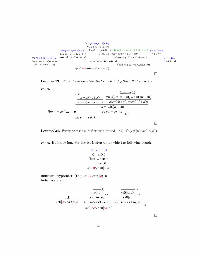
Lemma 33. From the assumption that a is odd it follows that sa is even

Proof.

∃ma = ss0.m+s0

(1)

s=ss0.b+s0sa=s(ss0.b+s0)

Lemma 32 :∀n s(ss0.n+s0)=ss0.(n+s0)

s(ss0.b+s0)=ss0.(b+s0)

sa=ss0.(n+s0)

∃k sa = ss0.k(1)

∃k sa = ss0.k

Lemma 34. Every number is either even or odd—i.e., ∀n(ss0|n∨ss0|n; s0)

Proof. By induction. For the basis step we provide the following proof:

∀xx.0 = 00=ss0.0∃m 0=ss0.m

i.e., ss0|0ss0|0∨ss0|0; s0

Inductive Hypothesis (IH): ss0|a∨ss0|a; s0Inductive Step:

IH:ss0|a∨ss0|a; s0

(1)

ss0|aL6

ss0|sa; s0

ss0|sa∨ss0|sa; s0

(1)

ss0|a; s0L33

ss0|sass0|sa∨ss0|sa; s0

(1)

ss0|sa∨ss0|sa; s0

31

Lemma 35. Given any two numbers, neither one when doubled is doublethe other plus 1. In symbols:

∀m∀n(¬(2.m = 2.n+ 1) ∧ ¬(2.m+ 1 = 2.n))

Proof. By induction on m. For the basis we need to prove

∀n(¬(2.0 = 2.n+ 1) ∧ ¬(2.0 + 1 = 2.n))

We invoke the abbreviations

Ψ(b, k) : ¬(ss0.k + s0 = ss0.b)

Φ(b, k) : ¬(ss0.k = ss0.b+ s0)

So the basis has the form

∀n(Φ(n, 0) ∧Ψ(n, 0))

The inductive step in the proof will have the overall form

∀n(Φ(n, k) ∧Ψ(n, k))

(3)

Φ(b, k) ∧Ψ(b, k)

(1)

Φ(b, k)Σ

Ψ(b, sk)(1)

Ψ(b, sk)(3)

Ψ(b, sk)

∀n(Φ(n, k) ∧Ψ(n, k))

(4)

Φ(b, k) ∧Ψ(b, k)

(2)

Ψ(b, k)Π

Φ(b, sk)(2)

Ψ(b, sk)(4)

Φ(b, sk)

Φ(b, sk) ∧Ψ(b, sk)

∀n(Φ(n, sk) ∧Ψ(n, sk))

The overall result, proved by induction, will therefore be

∀m∀n(Φ(n,m) ∧Ψ(n,m)),

that is,

∀m∀n(¬(ss0.m = ss0.n+ s0) ∧ ¬(ss0.m+ s0 = ss0.n)),

or, writing 1 for s0 and 2 for ss0,

∀m∀n(¬(2.m = 2.n+ 1) ∧ ¬(2.m+ 1 = 2.n)).

In words, as stated in the Lemma:

32

Given any two numbers, neither one when doubled is double theother plus 1.

We now have the task of providing the two embedded subproofs

∆,¬(ss0.k = ss0.b+ s0)︸︷︷︸Σ

¬(ss0.sk + s0 = ss0.b)

Γ,¬(ss0.k + s0 = ss0.b)︸︷︷︸Π

¬(ss0.sk = ss0.b+ s0)

for appropriate selections ∆ and Γ of axioms for arithmetic. As intimatedearlier, the axioms we use will be highlighted in blue. We present first theembedded subproof Π:

¬(ss0.k+s0=ss0.b)

∀x∀y x.sy=x.y+x


ss0.sk=ss0.k+ss0(1)

ss0.sk=ss0.b+s0(1)

ss0.k+ss0=ss0.b+s0


∀y s(ss0.k+y)=ss0.k+sy

s(ss0.k+s0)=ss0.k+ss0

s(ss0.k+s0)=ss0.b+s0


∀y s(ss0.b+y)=ss0.b+sy

s(ss0.b+0)=ss0.b+s0

s(ss0.k+s0)=s(ss0.b+0)

ss0.k+s0=ss0.b+0∀xx+0=x

ss0.b+0=ss0.b

ss0.k+s0=ss0.b

⊥ (1)

¬(ss0.sk=ss0.b+s0)

Finally we present the embedded subproof Σ:

¬(ss0.k=ss0.b+s0)

∀x∀y x.sy=x.y+x


ss0.sb=ss0.b+ss0(1)

ss0.k+s0=ss0.sb(1)

ss0.b+ss0=ss0.k+s0


∀y s(ss0.b+y)=ss0.b+sy

s(ss0.b+s0)=ss0.b+ss0

s(ss0.b+s0)=ss0.k+s0


∀y s(ss0.k+y)=ss0.k+sy

s(ss0.k+0)=ss0.k+s0

s(ss0.b+s0)=s(ss0.k+0)

ss0.b+s0=ss0.k+0∀xx+0=x

ss0.k+0=ss0.k

ss0.k=ss0.b+s0

⊥ (1)

¬(ss0.k+s0=ss0.sb)

33

Lemma 36. Every number is not both even and odd. In symbols:

∀x¬(Ex ∧Ox)

i.e.,∀x¬(∃y x=2y ∧ ∃z x=2z+1)

Proof. We use Lemma 35 as a premise in the following proof:

(1)

∃y x=2y ∧ ∃z x=2z+1

∃y x=2y

(1)

∃y x=2y ∧ ∃z x=2z+1

∃z x=2z+1

∀m∀n(¬(2m = 2n+1) ∧ ¬(2m+1 = 2n))

∀n(¬(2a = 2n+1) ∧ ¬(2a+1 = 2n))

¬(2a = 2b+1) ∧ ¬(2a+1 = 2b)

¬(2a = 2b+1)

(2)

c = 2a(3)

c = 2b+1

2a = 2b+1

⊥(1)

⊥(2)

⊥ (1)

¬(∃y c=2y ∧ ∃z c=2z+1)

∀x¬(∃y x=2y ∧ ∃z x=2z+1)

That use of Lemma 35 (which was proved by induction) does not makeLemma 35 into a cut sentence, for the reasons explained in §4.

Lemma 37. The square of an odd is odd. In symbols:

O(t)

O(t.t)

In proving this result, we shall make use of Associativity of Addition(Lemma 21), Commutativity of Multiplication (Lemma 23), Associativ-ity of Multiplication (Lemma 25), Distributivity (Lemma 24) and the factthat t.1=1 (Lemma 15). We shall avail ourselves of the usual abbreviatoryconventions in algebra, whereby, for example, the term

((ss0.m) + s0).((ss0.m) + s0)

is rendered more readably as

(2m+ 1)(2m+ 1).

34

That is, we often suppress multiplication signs and simply juxtapose the twomultiplicanda. Explicit dots (multiplication signs), however, have greaterscope than implicit ones. Thus ‘t.2m’, for example, is to be read as ‘t.(2.m)’.We also take successor to bind more tightly than multiplication, which inturn binds more tightly than addition. This enables us to use parenthesesless frequently. Order of arguments in operations matters, however, as does‘order of bracketing’.

35

Pro

of.

Th

eov

eral

lfo

rmof

the

form

alp

roof

is

O(t

),i.

e.,∃xt=

2x

+1

Π(2m

+1)

(2m

+1)

=2(m

[(2m

+1)

+1]

)+1

(1)

t=2m

+1

t.t=

2(m

[(2m

+1)

+1]

)+1

∃xt.t=

2x

+1(1)

∃xt.t=

2x

+1

i.e.

,O

(t.t

)

and

the

emb

edd

edsu

bp

roof

Π,

exp

loit

ing

the

abb

revia

tion

µ=

df

(2m

+1)

(2m

+1)

,is

Lemma

24:

(2m

+1)(2m

+1)=

(2m

+1)2m

+(2m

+1)1

Lemma

15:

(2m

+1)1

=2m

+1

µ=

(2m

+1)2m

+(2m

+1)

Lemma

21:

(2m

+1)2m

+(2m

+1)=

((2m

+1)2m

+2m

)+

1

µ=

((2m

+1)2m

+2m

)+

1Lemma

23:

(2m

+1)2m

=2m

(2m

+1)

µ=

(2m

(2m

+1)+

2m

)+

1Lemma

15:

2m.1

=2m

µ=

(2m

(2m

+1)+

2m.1)+

1Lemma

24:

2m

(2m

+1)+

2m.1

=2m

((2m

+1)+

1)

µ=

2m

((2m

+1)+

1)+

1Lemma

25:

2m

((2m

+1)+

1)=

2(m

[(2m

+1)+

1])

µ=

2(m

[(2m

+1)+

1])+

1

Lemma 38. The following is a valid argument-form:

Fht∀x(Fx ∨Gx)∀x¬(Fx ∧Gx)∀x(Gx→ Ghx)

Ft

Proof.

∀x¬(Fx∧Gx)

(2)

¬(Fht∧Ght)Fht

∀x(Gx→Ghx)

(3)

Gt→Ght

∀x(Fx∨Gx)

(5)

Ft∨Gt

(1)

¬Ft(5)

Ft

⊥(6)

Gt(6)

Gt(5)

Gt(4)

Ght(4)

Ght(3)

Ght

Fht∧Ght⊥

(2)

⊥ (1)

Ft

Lemma 39. Only evens have even squares. In symbols:

E(t.t)

E(t)

Proof. The proof is a substitution instance of the foregoing proof of Lemma 38.We have

Et.tLemma 34: ∀x(Ex ∨Ox)Lemma 36: ∀x¬(Ex ∧Ox)Lemma 37: ∀x(Ox→ Ohx)

Et

6.1 Complete Induction

In §4 we discussed what we called incremental Mathematical Induction. (Itis sometimes also called simple or weak induction.) There is a closely relatedprinciple to which we now turn, called complete or strong MathematicalInduction. The axiom schema in question is

∀x(∀y(y<x→Py)→Px)→ ∀zPz

37

6.1.1 Deriving Complete Induction

Lemma 40. Any proof Π using Complete Induction can be turned into aproof Π† using only incremental Mathematical Induction.

Proof. We proceed by induction in the metalanguage, on the complexity ofproofs Π. (So this induction, in the structural theory of proofs, has nothingto do with the two kinds of induction in formal arithmetic—complete andincremental—involved in the statement being proved.)

For the basis step: clearly if one is given a proof Π involving no applicationsof Complete Induction, then it can be turned (by doing nothing to it) intoa proof using only incremental Mathematical Induction. That is, for Π†

take Π.

Inductive hypothesis: Suppose the result holds for all proofs simpler thanthe proof Π under consideration.

Inductive Step: Show by cases that the result holds for Π. If the terminalstep of Π is an application of any rule other than →E with an instance ofComplete Induction as major premise, then the result obviously holds for Π.(For Π† take Π.) The only real work that needs to be done is when Π doesend with an application of →E that has as its major premise an instance ofComplete Induction. In such a case, Π takes the form

∀x(∀y(y<x→Py)→Px)→ ∀zPzΣ

∀x(∀y(y<x→Py)→Px)(1)

∀zPz

Here we can take the minor subproof Σ and embed it as follows, to producea proof Θ of P0.

Θ :

Σ∀x(∀y(y<x→Py)→Px)

∀y(y<0→Py)→P0

(1)

b<0i.e., ∃x 0=b+sx

(2)

0=b+sa


∀y b+sy=s(b+y)

b+sa=s(b+a)

0=s(b+a)

⊥(2)

⊥ (1)

b<0→Pb∀y(y<0→Py)

P0

38

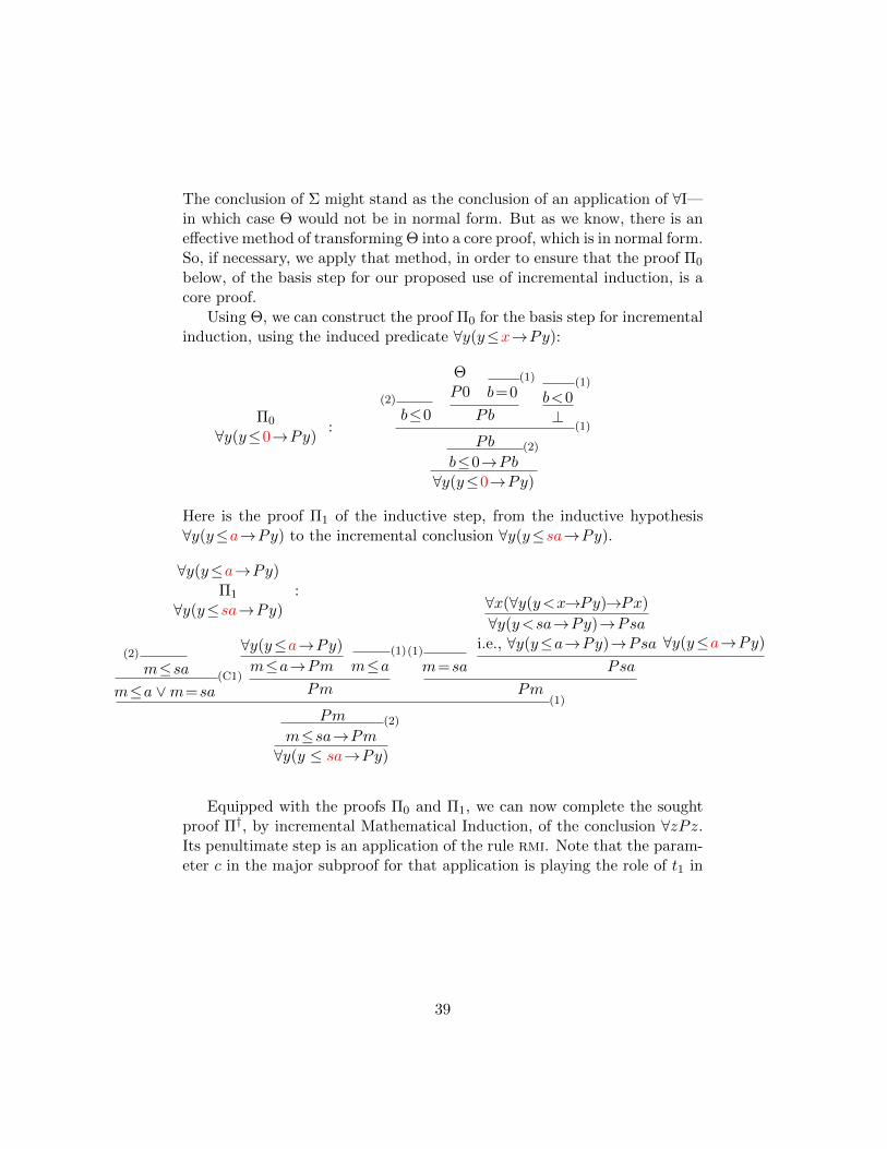
The conclusion of Σ might stand as the conclusion of an application of ∀I—in which case Θ would not be in normal form. But as we know, there is aneffective method of transforming Θ into a core proof, which is in normal form.So, if necessary, we apply that method, in order to ensure that the proof Π0

below, of the basis step for our proposed use of incremental induction, is acore proof.

Using Θ, we can construct the proof Π0 for the basis step for incrementalinduction, using the induced predicate ∀y(y≤x→Py):

Π0

∀y(y≤0→Py):

(2)

b≤0

ΘP0

(1)

b=0

Pb

(1)

b<0⊥

(1)

Pb (2)

b≤0→Pb∀y(y≤0→Py)

Here is the proof Π1 of the inductive step, from the inductive hypothesis∀y(y≤a→Py) to the incremental conclusion ∀y(y≤sa→Py).

∀y(y≤a→Py)Π1

∀y(y≤sa→Py):

(2)

m≤sa(C1)

m≤a ∨m=sa

∀y(y≤a→Py)

m≤a→Pm(1)

m≤aPm

(1)

m=sa

∀x(∀y(y<x→Py)→Px)

∀y(y<sa→Py)→Psai.e., ∀y(y≤a→Py)→Psa ∀y(y≤a→Py)

Psa

Pm(1)

Pm (2)

m≤sa→Pm∀y(y ≤ sa→Py)

Equipped with the proofs Π0 and Π1, we can now complete the soughtproof Π†, by incremental Mathematical Induction, of the conclusion ∀zPz.Its penultimate step is an application of the rule rmi. Note that the param-eter c in the major subproof for that application is playing the role of t1 in

39

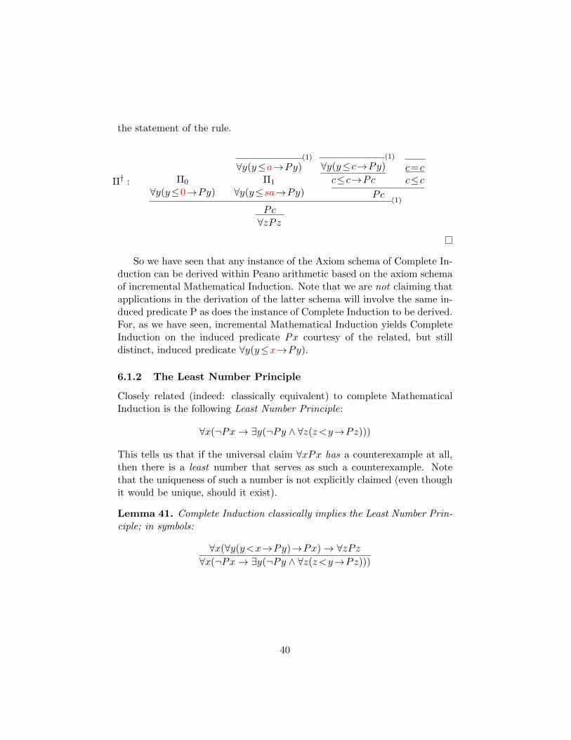
the statement of the rule.

Π† : Π0

∀y(y≤0→Py)

(1)

∀y(y≤a→Py)Π1

∀y(y≤sa→Py)

(1)

∀y(y≤c→Py)

c≤c→Pcc=cc≤c

Pc(1)

Pc∀zPz

So we have seen that any instance of the Axiom schema of Complete In-duction can be derived within Peano arithmetic based on the axiom schemaof incremental Mathematical Induction. Note that we are not claiming thatapplications in the derivation of the latter schema will involve the same in-duced predicate P as does the instance of Complete Induction to be derived.For, as we have seen, incremental Mathematical Induction yields CompleteInduction on the induced predicate Px courtesy of the related, but stilldistinct, induced predicate ∀y(y≤x→Py).

6.1.2 The Least Number Principle

Closely related (indeed: classically equivalent) to complete MathematicalInduction is the following Least Number Principle:

∀x(¬Px→ ∃y(¬Py ∧ ∀z(z<y→Pz)))

This tells us that if the universal claim ∀xPx has a counterexample at all,then there is a least number that serves as such a counterexample. Notethat the uniqueness of such a number is not explicitly claimed (even thoughit would be unique, should it exist).

Lemma 41. Complete Induction classically implies the Least Number Prin-ciple; in symbols:

∀x(∀y(y<x→Py)→Px)→ ∀zPz∀x(¬Px→ ∃y(¬Py ∧ ∀z(z<y→Pz)))

40

Proof. Steps of Classical Reductio are marked (1) and (3):

(4)

¬Pa

(3)

¬∃y(¬Py∧Qy)

(1)

¬Pa(2)

Qa

¬Pa∧Qa∃y(¬Py∧Qy)

⊥ (1)

Pa (2)

Qa→Pa

∀x(Qx→Px) ∀x(Qx→Px)→∀zPz∀zPzPa

⊥ (3)

∃y(¬Py∧Qy)

¬Pa→∃y(¬Py∧Qy)

∀z(¬Pz→∃y(¬Py∧Qy))

Now for Qx take ∀y(y<x→Py), in order to obtain the desired proof.If the predicate Px is effectively decidable, then the step marked (1)

is constructively acceptable. But the step marked (3) would then be anapplication of Markov’s Rule. For, given any natural number x, there areonly that many (finitely many) numbers y less than x that need to be checkedfor P -hood, in order to decide whether the complex predicate applies to x.So, if P (x) is effectively decidable, then so too is the slightly more complexpredicate Qx, i.e. ∀y(y<x→Py); whence also ¬Px∧∀y(y<x→Py). Thatwould make the existence of some x such that ¬Px ∧ ∀y(y<x→Py) a Σ0

1

matter.

Lemma 42. Provided that Px is effectively decidable, the Least NumberPrinciple constructively implies Complete Induction; in symbols:

∀x(¬Px→ ∃y(¬Py ∧ ∀z(z<y→Pz)))

∀x(∀y(y<x→Py)→Px)→ ∀zPz

Proof. Once again let the formula ∀y(y < x→ Py) be abbreviated to Qx.Then the problem becomes that of proving the argument

∀x(¬Px→∃y(¬Py∧Qy))

∀x(Qx→Px)→∀zPz

41

The following proof uses Classical Reductio just once, at the step marked (2).It is constructively acceptable if Px is effectively decidable.

(2)

¬Pa∀x(¬Px→∃y(¬Py∧Qy))

¬Pa→∃y(¬Py ∧Qy)

∃y(¬Py ∧Qy)

(1)

¬Pb ∧QbQb

(3)

∀x(Qx→Px)

Qb→Pb

Pb

(1)

¬Pb ∧Qb¬Pb

⊥(1)

⊥ (2)

Pa∀zPz (3)

∀x(Qx→Px)→∀zPz

7 The main argument, given informally

Suppose pq =√

2 — equivalently, p2 = 2.q2 for some non-zero q. We shallderive a contradiction. Consider the property Px that p is being supposedto enjoy:

∃y(y 6=0 ∧ x.x=2.(y.y))

We shall show that the assumption Pa, for arbitrary a, leads to a contra-diction.

So suppose Pa. By the Least Number Principle there is a least number ywith property P :

∃y(Py ∧ ∀z(z<y→¬Pz))

Let λ be such a number; that is, suppose we have

Pλ ∧ ∀z(z<λ→¬Pz)

Assuming nothing else about λ, we shall derive a contradiction.Pλ means that

∃y(y 6=0 ∧ λ.λ=2.(y.y))

Let µ be such a number:

µ 6=0 ∧ λ.λ=2.(µ.µ)

Since µ is non-zero, so too is 2.(µ.µ); whence also λ.λ is non-zero. It followsthat λ itself is non-zero:

λ 6= 0

42

Also, λ.λ is even. By Lemma 39 it follows that λ itself is even:

∃y λ=2.y

Suppose that ρ is such a number:

λ=2.ρ

Since λ is non-zero, so too is ρ :

ρ 6=0

By Lemma 31,ρ<λ

Recall that we haveλ.λ=2.(µ.µ)

Substituting 2.ρ for λ, we obtain

(2.ρ).(2.ρ)=2.(µ.µ)

By Lemma 29 we haveµ.µ=2.(ρ.ρ),

whence, by Lemma 39, µ itself is even:

∃y µ=2.y

Let σ be such a number:µ=2.σ

So we have(2.σ).(2.σ)=2.(ρ.ρ),

whence by Lemma 29 again we have

ρ.ρ=2.(σ.σ)

Since µ is non-zero, so too is σ:

σ 6=0

So we haveσ 6=0 ∧ ρ.ρ=2.(σ.σ),

43

whence∃y(y 6=0 ∧ ρ.ρ=2.(y.y))

Recall that we are supposing

Pλ ∧ ∀z(z<λ→¬Pz)

So we have∀z(z<λ→¬Pz)

Instantiating with respect to ρ, we have

ρ<λ→¬Pρ

It follows that¬Pρ,

i.e.¬∃y(y 6=0 ∧ ρ.ρ=2.(y.y)).

Contradiction.

8 The main argument, given formally

Theorem 1. ∀x¬∃y(y 6=0 ∧ x.x=2.(y.y))

Proof. We seek to show∀x¬Px

wherePx ≡df ∃y(y 6=0 ∧ x.x=2.(y.y))

Overall, the formal proof will be of the following form:

Least Number Principle :∀x(Px→∃y(Py∧∀z(z<y→¬Pz)))

(2)

Pa→∃y(Py∧∀z(z<y→¬Pz))(1)

Pa

(3)

∃y(Py∧∀z(z<y→¬Pz))

(4)

Pλ∧∀z(z<λ→¬Pz)Σ⊥

(1)

⊥(3)

⊥(2)

⊥ (1)

¬Pa∀x¬Px

44

Clearly for the construction of the outstanding embedded proof Σ it willsuffice to find a proof of the form

Pλ , ∀z(z<λ→¬Pz)︸︷︷︸Π⊥

The following can serve as Π, provided we can supply its embedded sub-proof Ω. Note that within this display of Π we can see only the parametersλ, µ and ρ invoked. The role of the parameter σ is confined to the embeddedsubproof Ω.

Pλi.e., ∃y(y 6=0∧λ.λ=2.(y.y))

(1)

µ 6=0∧λ.λ=2.(µ.µ)

λ.λ=2.(µ.µ)L39

∃y λ=2.y

∀z(z<λ→¬Pz)

(3)

ρ<λ→¬Pρ

(2)

λ=2.ρ

(2)

λ=2.ρ

(1)

µ 6=0∧λ.λ=2.(µ.µ)L30

λ.λ 6=0L4

λ 6=0L5

ρ 6=0L31

ρ<λ

(4)

¬Pρ

(2)

λ=2.ρ ,(1)

µ 6=0∧λ.λ=2.(µ.µ)︸︷︷︸Ω

Pρ : ∃y(y 6=0 ∧ ρ.ρ=2.(y.y))

⊥(4)

⊥(3)

⊥(2)

⊥(1)

⊥

Finally we supply the embedded subproof Ω:

µ 6=0 ∧ λ.λ=2.(µ.µ)

λ.λ=2.(µ.µ) λ=2.ρ

(2.ρ).(2.ρ)=2.(µ.µ)L29

µ.µ=2.(ρ.ρ)L39

∃y µ=2.y

µ 6=0 ∧ λ.λ=2.(µ.µ)

µ 6=0(1)

µ=2.σ

σ 6=0

µ 6=0 ∧ λ.λ=2.(µ.µ)

λ.λ=2.(µ.µ) λ=2.ρ

(2.ρ).(2.ρ)=2.(µ.µ)L29

µ.µ=2.(ρ.ρ)(1)

µ=2.σ

(2.σ).(2.σ)=2.(ρ.ρ)L29

ρ.ρ=2.(σ.σ)

σ 6=0 ∧ ρ.ρ=2.(σ.σ)

∃y(y 6=0 ∧ ρ.ρ=2.(y.y))(1)

∃y(y 6=0 ∧ ρ.ρ=2.(y.y))

References

Neil Tennant. Cut for Core Logic. Review of Symbolic Logic, 5(3):450–479,2012.

45

Neil Tennant. Cut for Classical Core Logic. Review of Symbolic Logic, 8(2):236–256, 2015a.

Neil Tennant. The Relevance of Premises to Conclusions of Core Proofs.Review of Symbolic Logic, 8(4):743–784, 2015b.

46

pythagoras meets peano, courtesy of core logic

Documents