qctachart - technical analysis charting tools -...
TRANSCRIPT

Technical Analysis Charting for Stocks
QCTAChart
Contact Information
Company Web Site: http:// www.quinn-curtis.com
General Information: [email protected]: [email protected]
Technical Support Forum
http://quinn-curtis.com/index.php/forumframe/
Revision Date 3/25/2017 Rev. 2.5
Documentation and Software Copyright Quinn-Curtis, Inc. 2017

Quinn-Curtis, Inc. END-USER LICENSE AGREEMENT
This End User License Agreement (“Agreement”) is between you and QCTAChart and governs use of this app madeavailable through the a distributor (Apple, Microsoft, Google, Amazon, etc.) App store. By installing the QCTAChart App, you agree to be bound by this Agreement and understand that there is no tolerance for objectionable content. If you do not agree with the terms and conditions of this Agreement, you are not entitled to use the QCTAChart App.<
In order to ensure QCTAChart provides the best experience possible for everyone, we strongly enforce a no tolerance policy for objectionable content. If you see inappropriate content, please use the "Report as offensive" feature found under each post.
1. Parties This Agreement is between you and QCTAChart only, and not the App distributor. Notwithstanding the foregoing, you acknowledge that the App distributor and its subsidiaries are third party beneficiaries of this Agreement and the App distributor has the right to enforce this Agreement against you. QCTAChart, not the App distributor, is solely responsible for the QCTAChart App and its content.
2. Privacy QCTAChart may collect and use information about your usage of the QCTAChart App, including certain types of information from and about your device. QCTAChart may use this information, as long as it is in a form that does not personally identify you, to measure the use and performance of the QCTAChart App.
3. Limited License QCTAChart grants you a limited, non-exclusive, non-transferable, revocable license to use theQCTAChart App for your personal, non-commercial purposes. You may only use theQCTAChart App on the App distributor devices that you own or control and as permitted by the App Store Terms of Service.
4. Objectionable Content Policy Content may not be submitted to QCTAChart, who will moderate all content and ultimately decide whether or not to post a submission to the extent such content includes, is in conjunction with, or alongside any, Objectionable Content. Objectionable Content includes, but is not limited to: (i) sexually explicit materials; (ii) obscene, defamatory, libelous, slanderous, violent and/or unlawful content or profanity; (iii) content that infringes upon the rights of any third party, including copyright, trademark, privacy, publicity or other personal or proprietary right, or that is deceptive or fraudulent; (iv) content that promotes the use or sale of illegal or regulated substances, tobacco products, ammunition and/or firearms; and (v) gambling, including without limitation,any online casino, sports books, bingo or poker.
5. Warranty QCTAChart disclaims all warranties about the QCTAChart App to the fullest extent permitted by law. To the extent any warranty exists under law that cannot be disclaimed, QCTAChart, not the App distributor, shall besolely responsible for such warranty.
6. Maintenance and Support QCTAChart does provide minimal maintenance or support for it but not to the extent that any maintenance or support is required by applicable law, QCTAChart, not the App distributor, shall be obligated to furnish any such maintenance or support.
7. Product Claims QCTAChart, not the App distributor, is responsible for addressing any claims by you relating to the QCTAChart App or use of it, including, but not limited to: (i) any product liability claim; (ii) any claim that the QCTAChart App fails to conform to any applicable legal or regulatory requirement; and (iii) any claim arising underconsumer protection or similar legislation. Nothing in this Agreement shall be deemed an admission that you may have such claims.
8. Third Party Intellectual Property Claims QCTAChart shall not be obligated to indemnify or defend you with respect to any third party claim arising out or relating to the QCTAChart App. To the extent QCTAChart is required to provide indemnification by applicable law, QCTAChart, not the App distributor, shall be solely responsible for the investigation, defense, settlement and discharge of any claim that the QCTAChart App or your use of it infringesany third party intellectual property right.
ii

9. RESTRICTIONS. You may not reverse engineer, de-compile, or disassemble the SOFTWARE, except and only to the extent that such activity is expressly permitted by applicable law notwithstanding this limitation. You may notrent, lease, or lend the SOFTWARE. You may not use the SOFTWARE to perform any illegal purpose.
10. SUPPORT SERVICES. Quinn-Curtis, Inc. may provide you with support services related to the SOFTWARE. Use of Support Services is governed by the Quinn-Curtis, Inc. polices and programs described in the user manual, inonline documentation, and/or other Quinn-Curtis, Inc.-provided materials, as they may be modified from time to time. Any supplemental SOFTWARE code provided to you as part of the Support Services shall be considered part of the SOFTWARE and subject to the terms and conditions of this EULA. With respect to technical information youprovide to Quinn-Curtis, Inc. as part of the Support Services, Quinn-Curtis, Inc. may use such information for its business purposes, including for product support and development. Quinn-Curtis, Inc. will not utilize such technical information in a form that personally identifies you.
11. TERMINATION. Without prejudice to any other rights, Quinn-Curtis, Inc. may terminate this EULA if you failto comply with the terms and conditions of this EULA. In such event, you must destroy all copies of the SOFTWARE.
12. COPYRIGHT. The SOFTWARE is protected by United States copyright law and international treaty provisions. You acknowledge that no title to the intellectual property in the SOFTWARE is transferred to you. You further acknowledge that title and full ownership rights to the SOFTWARE will remain the exclusive property of Quinn-Curtis, Inc. and you will not acquire any rights to the SOFTWARE except as expressly set forth in this license. You agree that any copies of the SOFTWARE will contain the same proprietary notices which appear on and in the SOFTWARE.
13. EXPORT RESTRICTIONS. You agree that you will not export or re-export the SOFTWARE to any country, person, entity, or end user subject to U.S.A. export restrictions. Restricted countries currently include, but are not necessarily limited to Cuba, Iran, Iraq, Libya, North Korea, Sudan, and Syria. You warrant and represent that neitherthe U.S.A. Bureau of Export Administration nor any other federal agency has suspended, revoked or denied your export privileges.
14. LIMITATION OF LIABILITY. IN NO EVENT SHALL QUINN-CURTIS, INC. OR ITS SUPPLIERS BE LIABLE TO YOU FOR ANY CONSEQUENTIAL, SPECIAL, INCIDENTAL, OR INDIRECT DAMAGES OF ANY KIND ARISING OUT OF THE DELIVERY, PERFORMANCE, OR USE OF THE SUCH DAMAGES. IN ANY EVENT, QUINN-CURTIS’S LIABILITY FOR ANY CLAIM, WHETHER IN CONTRACT, TORT, OR ANY OTHER THEORY OF LIABILITY WILL NOT EXCEED THE GREATER OF U.S. $1.00 OR LICENSE FEE PAID BY YOU.
15. U.S. GOVERNMENT RESTRICTED RIGHTS. The SOFTWARE is provided with RESTRICTED RIGHTS. Use, duplication, or disclosure by the Government is subject to restrictions as set forth in subparagraph (c)(1)(ii) of The Rights in Technical Data and Computer SOFTWARE clause of DFARS 252.227-7013 or subparagraphs (c)(i) and (2) of the Commercial Computer SOFTWARE- Restricted Rights at 48 CFR 52.227-19, as applicable. Manufacturer is: Quinn-Curtis, Inc., 18 Hearthstone Dr., Medfield MA 02052 USA.
16. MISCELLANEOUS. If you acquired the SOFTWARE in the United States, this EULA is governed by the laws of the state of Massachusetts. If you acquired the SOFTWARE outside of the United States, then local laws may apply.
Should you have any questions concerning this EULA, or if you desire to contact Quinn-Curtis, Inc. for any reason, please contact Quinn-Curtis, Inc. by mail at: Quinn-Curtis, Inc., 18 Hearthstone Dr., Medfield MA 02052 USA, or by telephone at: (508)359-6639, or by electronic mail at: [email protected].

Table of Contents1. Introduction ................................................................................................................................................................. 1
QCTAChart for Technical Analysis .......................................................................................................................... 1Financial Data Sources ............................................................................................................................................... 4Chapter Summary ....................................................................................................................................................... 5Customer Support ....................................................................................................................................................... 6
2. Using QCTAChart ...................................................................................................................................................... 7Event-based Coordinate System ................................................................................................................................ 9Stock Selection from the Portfolio ............................................................................................................................. 9Panning and zooming of data ................................................................................................................................... 10Y-Axis Scaling Options for the Primary Chart ........................................................................................................ 14Dynamic auto-scaling to displayed data ................................................................................................................... 15Data value or tooltip display .................................................................................................................................... 15Compare different stocks in the Primary Window ................................................................................................... 17Stock Selection ......................................................................................................................................................... 18
3. Define the Primary Chart .......................................................................................................................................... 21Classic Open-high-low-close plot ........................................................................................................................... 23Candlestick Plot ........................................................................................................................................................ 24Candlestick -Volume plot .......................................................................................................................................... 25Simple line plot of close values ................................................................................................................................ 27Mountain (or filled) close plot ................................................................................................................................. 29Bar plot ..................................................................................................................................................................... 29Scatter plot ................................................................................................................................................................ 30Point and Figure Charts ............................................................................................................................................ 31Renko Charts ............................................................................................................................................................ 33
4. Technical Indicator overlays for the Primary chart .................................................................................................. 35Simple moving averages .......................................................................................................................................... 35Exponential moving averages .................................................................................................................................. 37Moving Average Bands ............................................................................................................................................ 39Bollinger Bands ........................................................................................................................................................ 41Parabolic SAR .......................................................................................................................................................... 43
5. Secondary Chart Indicators ..................................................................................................................................... 47Adding Secondary Charts (Technical Indicators) .................................................................................................... 47Volume Indicators .................................................................................................................................................... 48Money Flow (MFI) ................................................................................................................................................... 49Relative Strength (RSI) ............................................................................................................................................ 52Williams %R ............................................................................................................................................................ 54Rate of Change (ROC) ............................................................................................................................................. 56Momentum (also known as the Change Indicator) .................................................................................................. 57Stochastic (Fast and Slow) ....................................................................................................................................... 59Moving Average Convergence/Divergence (MACD) ............................................................................................. 62Average Directional Indicator (ADX) ...................................................................................................................... 64
6. Technical Analysis Drawing Objects ....................................................................................................................... 67Trend Line ................................................................................................................................................................ 68Horizontal and Vertical data markers ....................................................................................................................... 69Fibonacci Overlay .................................................................................................................................................... 70Labels for Annotation ............................................................................................................................................... 72Arrows for Annotation ............................................................................................................................................. 74
7. Point and Figure Charts ............................................................................................................................................. 77Point and Figure y-Axis Scale Modes ...................................................................................................................... 78Point And Figure Setup Options .............................................................................................................................. 82
8. Renko Charts ............................................................................................................................................................. 89Renko y-Axis Scale Modes ...................................................................................................................................... 89 .................................................................................................................................................................................. 91
iv

Renko Chart Setup Options ...................................................................................................................................... 919. Miscellaneous Setup Items ........................................................................................................................................ 9510. File and Printer Rendering ..................................................................................................................................... 99
Printing a Chart ........................................................................................................................................................ 99Capturing the Chart as an Image ............................................................................................................................ 100
Index ............................................................................................................................................................................ 103 ..................................................................................................................................................................................... 107

Technical Analysis Charting for Stocks - QCTAChart
7

1. Introduction
Technical Analysis of stocks, bonds, commodities and other securities, is the art of predicting future price movements (for the security) based on the study of past price and volume movements. Starting with historical Open-high-low-close-volume data for a given security, technical analysis consists of applying one or more functions to that data, creating an indicator which predicts the future trend of the security, whether it be up, down or flat. Buy and sell actions for the security are then decided based on the indicator.
That's it in a nutshell. The defining postulate of technical analysis is that the historical market action of a security takes into account everything publicly known about the security. There is no need for the technicaltrader to study a stocks balance sheet, income statement, cash flow, or recent product announcements (the bread and butter of a competing strategy known as fundamental analysis), because all of these things are already factored in the stocks price. This assumes that the security trades in a free market, where the price action is controlled by thousands, or even millions of independent buyers and sellers, all operating using their own criteria. Don't expect technical analysis to work for securities which have an extremely small float (penny stocks for example), or are largely controlled by a single trading entity (stock trading scams where the price is manipulated by a coordinated network of brokers, buyers and sellers – think the Wolf of Wall Street), or in stock exchanges run by countries which to not believe in free market economics and are willing to manipulate a stock price to their own end.
Technical analysis does not require that the practitioner use charting. It is straightforward to use technical analysis to produce buy, hold and sell signals, without ever looking at a chart. The computer allows a skilled programmer to automate the analysis of historical stock data, and produce buy and sell signals usingtechnical analysis without the user every seeing a Open-high-low-close chart, or a technical indicator chart. Traders involved in computer-driven trading will execute trades based on a computer generated buy or sell signal. In this case the program is processing technical indicators derived from the fundamental Open-high-low-close-volume data, and looking for specific buy and sell signals.
QCTAChart for Technical AnalysisThe QCTAChart software package is for those who do want to use charting as part of their decision making process. Typically, a user will choose a stock, and a time frame to analyze. The historical stock data will be displayed as an Open-high-low-close chart (or candlestick chart). The user will have the optiona applying a selection of time-invariant transfer functions to the data, producing additional charts which will indicate buy or sell signals on inspection. In some cases, an indicator will overlay the existing Open-high-low-close chart, and in others they will be displayed in a synchronized window under the main Open-high-low-close chart.
A QCTAChart has three major major plotting areas: a zoom window, a primary chart window, and secondary indicator window area consisting of one or more charts. A typical QCTAChart is shown below. The small chart at the top is the zoom control for the next chart, which is the primary technical chart window. The smaller windows under that the are the secondary technical indicators.
1

1. Introduction
This chart combines a zoom window, a Primary OHLC chart displaying a Parabolic SAR overlay, and two Secondary charts displaying a Volume bar graph, and a Slow Stochastic indicator chart.
Primary Chart Window
The Primary chart window can display the OHLC stock data for up to three stocks using the following plot options:
Classic Open-high-low-close
Candlestick
Simple line plot, scatter plot or bar plot of close data
Mountain (or filled) line plot of close data
Candlestick-Volume candlestick plot
Open-High-Low-Close Bar plot
Point and Figure plot
Renko plot
Time frame (starting date/time and frame extent is controlled using a dedicated zoom control window
Data values for the plot, at the intersection of a mouse controlled vertical cursor with the plot, are displayedabove each chart window
You can also overlay the Primary chart using one or more of the following technical indicators
2

Technical Analysis Charting for Stocks - QCTAChart
Simple moving averages
Exponential moving averages
Moving Average Bands
Bollinger Bands
Parabolic SAR
Some the other options associated with the Primary chart are:
Dynamic auto-scaling to displayed data
Compare up to three different stocks
Linear, Logarithmic, and Normalized y-axis scale
Synchronize scrolling (panning) and zooming of all chart windows
Financial Chart objects which can be dropped into a chart
◦ Horizontal and Vertical data makers
◦ Fibonacci overlay
◦ Labels for Annotation
◦ Trend lines
◦ Arrows
Secondary Chart Window
The Secondary window can display the following technical indicators:
Average Directional Indicator
Momentum
Rate of Change (ROC)
Relative Strength (RSI)
Stochastic (Fast and Slow)
Williams %R
Moving Average Convergence/Divergence (MACD)
3

1. Introduction
Volume charts
Integrated Dialog Boxes
There are Primary Chart, Primary Chart Technical Indicators, Secondary Chart, General Chart characteristic, Drawing Tools and Portfolio dialog boxes which are invoked with small buttons on the main view page. The end-user can customize which stocks and technical indicators are displayed. Plot attributes (plot type, line and fill colors,line thickness), text fonts and text sizes are all adjustable.
Serialization
The program remembers your last setup and loads that when it starts.
Financial Data Sources
Paid Data Sources
A technical analysis charting package means little if you do not have a source of historical data for the securities youwant to analyze. There are many sources of paid historical data. If you work for a large financial company, you may have access to computer feeds from Thompson Reuters, Bloomberg, Wall Street Journal, Metastock and many others. You can get historical data in file form, and on-line. Since data in file form must be constantly updated in order to keep it current, the best source is going to be on-line. Paid, online, data sources are going to cost anywhere from hundreds, to tens of thousands of dollars per year, depending on how many financial instruments you have access to (there are tens of thousands), how many historical data sets a day you expect to retrieve, and the frequency of the historical data (end-of-day (EOD) data, minute by minute, 5-second, or even tick by tick. This software is designed to work with any frequency of data. What we don't have at this time are drivers for these paid, historical data feeds. Should you provide us with a specification, for the URL query, and the return data format, we can probably create a custom data source module for you which will let you read data from that data source for little or no money.
Free Data Sources
There are several, free, real-time URL sources of historical stock data. These are Yahoo Finance, Google Finance, and Quandl. The use of historical data from these sources is completely free. What you can't do is download historical data from them (it's free after all) and then sell, or give it away to someone else. That would be a copyrightviolation. But, you can use the data in your stock trading program(s) to make decisions about when to buy or sell stocks, without paying them any royalties. Most of the historical stock data is end-of-day (EOD) data. It can go backtwenty or thirty years for some stocks. Yahoo and Google also offer intra-day data (stock prices throughout a tradingday) going back up to twenty days. The frequency of the data (whether or not it is minute by minute data, or some multiple thereof, varies.
There are some issues with the free historical data sources. In most cases, once you go back ten or fifteen years, the Open-high-low-close-volume format of data degrades to just daily Close-Volume data, and finally to just the close price for the security. So technical indicators which depend on Open, High, Low and Volume values can't be used for the time range in those case. Also, historical data is dependent on stock splits, and some data sources normalize the stock data for stock splits and others don't. When the free data sources do adjust the OHLC data for stock splits, it often takes a month or two after the split occurs. Until that time, charts of the stock will show a drastic price drop on the date of the stock split, since that is what the data will show. During that update interval, before the historical data has been normalized for the stock splits, technical analysis will not be practical. This was more of an issue
4

Technical Analysis Charting for Stocks - QCTAChart
fifteen years ago, where high growth stocks split every one or two years, not so much now. Apple (AAPL) recently split though so watch out for that. Paid data sources such as Thompson Reuters are always going to have better, more update to date data, with complete Open-high-low-close data and data always properly normalized for stock splits.
Yahoo Finance
Yahoo Finance is a web site that provides current and historical financial information on USA and many non-USA markets. This includes quotes on stocks, bonds, commodities and futures. There terms of use for using this data in third party programs, rather than those available on the Yahoo web site, are vague and hard to find.
Google Finance (now discontinued)
Google Finance, launched in 2006, was meant to be a competitor to Yahoo Finance. It offered much the same as Yahoo in terms of current and historical data for stocks, bonds, commodities and stock futures. Unfortunately, Google announced in 2013 that they were discontinuing most of Google Finance. However, the current, and historical data quote service, still seems to be working.
Quandl
Compared to Google and Yahoo, Quandl is a relatively new data source, started a few of years ago. The site offers access to several million financial, economic and social datasets, including EOD data for a large number of USA and non-USA stocks. We bulk download the Quandl Wiki stock and index database every evening, then run our own programs on it to squeeze every extraneous byte out of the data which QCTAChart won't use. When you view data using QCTAChart, your are acquiring the stock data from the Quinn-curtis servers. But it is originally sourced from Quandl.
Chapter Summary
Chapter 1 – this chapter.
Chapter 2 – describes how the main screen UI works with the mouse and touch screen, and how to add your our own stocks to a portfolio.
Chapter 3 - the Primary Chart setup dialog defines which stocks from the current portfolio are plotted, and the plot type and setup options used. Plot types include OHLC, Candlestick, Line, Mountain, Bar, Scatter (or Symbol), Candlestick-Volume, OHLC-Bar, Renko and Point & Figure plots.
Chapter 4 - how to add technical indicators as overlays to the Primary chart. Technical indicators include up to twoMoving Average plots, up to two Exponential Moving Average plots, Bollinger Bands, Moving Average Bands, andthe Parabolic SAR indicator.
Chapter 5 - how to add technical indicators as Secondary charts. Secondary chart technical indicators include: Volume, Volume Moving Average, Money Flow, (RSI) Relative Strength, (%R) Williams, (ROC) Rate of Change, Momentum, Stochastic, MACD and (ADX) Average Directional Change.
Chapter 6 – how to use the drawing tools to add text, labels, horizontal and vertical markers, trend lines, arrows and Fibonacci levels to the Primary chart.
Chapter 7 – discusses the Point and Figure chart in more detail.
5

1. Introduction
Chapter 8 - discusses the Renko chart in more detail.
Chapter 9 – covers the General chart setup dialog. This setup dialog allows the user to specify options controlling the overall look of the chart display. The user can specify the colors used in the chart, along with line widths, the text sizes and the overall text font. An option is included to use the European convention for dates (dd/mm/yy), then than the default US convention (mm/dd/yy).
Chapter 10 – Printing and Saving a chart as an image file is covered.
Customer SupportUse our forum http://quinn-curtis.com/index.php/forumframe/ at for customer support.
6

2. Using QCTAChart
QCTAChart is customized using a collection of dialogs. The dialogs are invoked by pressing one of the buttons place along the periphery of the chart.
A summary of the interactions the user can have with the chart
Portfolio of Stocks - Select one of five portfolios you can maintain with up to 20 stocks each.
Zoom In at current position- Decrease the x-axis time scale to show fewer data points.
Zoom Out at current position - Increase the x-axis time scale to show more data points.
Primary Chart Stocks - Select the main stock for the primary chart, and optionally, compare it to up to two other stocks. Options include displaying the plots in OHLC, Candlestick, Line, Mountain, Bar, Scatter (or Symbol), Candlestick-Volume, OHLC-Bar, Renko and Point & Figure plots. Renko and Point & Figure plots are restricted to the first (or main) plot of the primary chart.
Primary Chart Technical Indicators - The primary chart supports a standard set of technical indicators, overlaid directly on top of the primary chart plots. Technical indicators include up to two Moving Average plots, up to two Exponential Moving Average plots, Bollinger Bands, Moving Average Bands, and the Parabolic SAR indicator.
Secondary Chart Technical Indicators - There can be one or more secondary charts, displaying standalone technical indicators, synchronized with the plots in the primary chart window. The number of secondary charts is limited by the amount space your device screen has for the app. If you keep adding secondary chart technical indicators, the secondary charts will be forced in a smaller and smaller area, making them unreadable. The secondary chart technical indicators always refer back to the first (or main) plot of the primary chart. Secondary chart technical indicators include: Volume, Volume Moving Average,
7

2. Using QCTAChart
Money Flow, (RSI) Relative Strength, (%R) Williams, (ROC) Rate of Change, Momentum, Stochastic, MACD and (ADX) Average Directional Change.
Primary Chart Drawing Tools - The primary chart can be marked up using a collection of technical indicator objects. These include Text (does not scroll with the data), Labels (scrolls with the data), Horizontal Marker, Vertical Marker, Trend Line, Arrow and Fibonacci Levels.
General Chart Setup - This setup dialog allows the user to specify options controlling the overall look of the chart display. The user can specify the colors used in the chart, along with line widths, the text sizes and the overall text font. An option is included to use the European convention for dates (dd/mm/yy), then than the default US convention (mm/dd/yy) .
Printing - Print the current chart to an available printer.
Saving Image to a File - Save an image of the chart to local storage.
Squeeze Secondary Charts - Minimize the top and bottom margin of the secondary charts to make more room for the plotting area of each chart.
Un-Squeeze Secondary Charts - Return the secondary charts to the default margin between charts.
Help - This file.
Depending on whether or not you are using a desktop PC with a wide screen, or a laptop, a tablet, a phone, or some other mobile device, the screen may vary in size. In order to accommodate screens of limited resolution, and save space, some of the dialog buttons are removed from the chart, and instead are displayed in a tool bar on the left side of the screen.
On mobile devices of limited resolution (< 1200 dpi horizontal), some of the buttons are only available on the left-most toolbar.
In the example above, the Stock Portfolio button, , has been moved down and to the left. It's also found in the toolbar on the left. The General Chart Setup button, , and the Printer button, , are found in the toolbar on the
8

Technical Analysis Charting for Stocks - QCTAChart
left. Given the limited real-estate, the Secondary chart Squeeze option, , is always on.
When run on a screen of limited resolution, the list of stocks symbols at the top of the chart may be reduced to fit onthe screen. In this case it is possible to select non-visible stock symbols using the First Plot combo boxes in the Primary Chart setup dialog, invoke using the button.
Event-based Coordinate SystemThis software makes use of an event-based coordinate system. In event-based plotting, the coordinate system is scaled to the number of event objects. Each event object represents an x-value, and one or more y-values. The x-value can be time based, or numeric based, while the y-values are numeric based. Since an event object can represent one or more y-values for a single x-value, it can be used as the source for simple plot types (simple line plot, simple bar plot, simple scatter plot, simple line marker plot) and group plot types (open-high-low-close plots, candlestick plots, group bars, stacked bars, etc.). The most common use for event-based plotting is for displaying time-based data which is discontinuous: financial markets data for example. In financial markets, the number tradinghours in a day may change, and the actual trading days. Weekends, holidays, and unused portions of the day can be excluded from the plot scale, producing continuous plots of discontinuous data.
An event-based coordinate system plots data points equally spaced, regardless of the time stamp. Data plots smoothly transition off-hours, weekends and holidays.
Above is a plot of the OHLC data for INTC (Intel) over the December 2013 Christmas holiday. Note that the only dates included are the trading dates (12/23, 12/24, 12/26, 12/27, 12/30, 12/31, 1 /2 /2014, etc. The non-trading days of 12/25, 12/28, 12/29, 1/1/2104 are not included in the charts coordinate system. The coordinate system is defined by the data contained within. If for some reason you did have data for 12/25/2104, if it was included in the OHLC data source, it would be included in the scale.
Stock Selection from the PortfolioThe stocks in the current portfolio are listed across the top of the screen, to the right of the Portfolio combo box and
9

2. Using QCTAChart
the , symbol. The stock being analyzed is highlighted with a box drawn around it, TXN in the example below.
You can change the current stock by clicking (touching) the symbol for one of the other stocks. All of the charts willbe updated to reflect the stock change. You can also change the current stock using the Primary Chart setup dialog, under the First Plot. Section.
Panning and zooming of dataStock data is downloaded into the software using one of three different time-frames: 3-year, 10-year, or 30-year. Many stocks do not have 30 years of history to download and in that case the stock data is truncated to the first recorded stock date. The default time frame is 3-years for mobile devices and 10-years for all others. But, you can override the default setting at any time using the Primary Chart setup dialog, . There you will find the following selection:
Select the maximum download range you want. This value represents the maximum download range, so you cannot zoom to display earlier than the downloaded range, unless you change this setting. This value is a global setting and applies to all stocks in all portfolios. The larger the maximum download range, the longer it takes to download the data from the internet and the longer it takes for most all forms of display.
You can zoom in on any time segment within the downloaded range of values. So if you have downloaded 10 years of data, you can view any time frame from one week to 10 years. The stock data is daily open-high-low-close and volume values, so you can't zoom into intra-day ticker values.
The primary zoom tool for the stock data in the Primary chart is the zoom window, which the top-most plot above the primary chart.
10

Technical Analysis Charting for Stocks - QCTAChart
Use the zoom rectangle to set the starting and ending dates of the Primary and Secondary chart windows.
The full scale of the zoom window represents the (3-, 10- or 30-year) value you selected in the Maximum Download Range option of the Primary Chart setup. The transparent, blue, rectangle (called the zoom rectangle) inside that range represents the range of data displayed in the Primary Chart. There are three interactions you can make with the zoom rectangle.
First, you can click and drag (or touch and slide) the center of the zoom rectangle and move it back and forth within the full scale range of the Zoom Window. This keeps the same range of values (6 months worth of data for example) while changing the starting and ending dates of the Primary and Secondary charts.
Click and drag (or touch and slide) the center of the Zoom rectangle to control the Primary charts position without changing the range
Second, you can click and drag ( or touch and slide) on either the left edge, or the right edge of the zoom rectangle. This will change the starting date (left edge) and ending date (right edge) of the zoom rectangle, while also affecting the zoom range and equivalent amount.
11

2. Using QCTAChart
Click and drag (or touch and slide) the left or right edges of the Zoom rectangle to control the Primary charts starting and ending position
Zoom In at current position
Zoom Out at current position
Also, there are buttons for zooming on the left and right of the Zoom window” Zoom In and Zoom Out. For each press, the Zoom In button will reduce the range of the Zoom rectangle by one half. The Zoom Out button will double the range of the Zoom rectangle. If the left and right edges of the Zoom rectangle do not touch the minimum or maximum bounds of the Zoom window, the resulting new range is centered on the same date as the previous zoom rectangle. If however a left or right edge of the Zoom rectangle is touching the minimum or maximum bounds of the zoom rectangle, that edge sticks to the minimum or maximum boundary of the Zoom window and the starting or ending bounds of the zoom rectangle is adjusted to reflect the new range, which is still halved or double with eachZoom In or Zoom out press.
You can also click and drag (or touch and slide) on the Primary chart to pan the data left of right. Choose and area ofthe Primary chart where there is no data, so that the action is not confused with the tooltip mode. The graph is not updated until you the drag operation completes.
Starting Position
12

Technical Analysis Charting for Stocks - QCTAChart
The Zoom In button was pressed 4 times, reducing the x-axis time scale by 16 times
The Secondary charts are always synced to the Zoom window, and therefore the Primary chart. When the time frame of the Primary chart changes, so will the time frame of the Secondary charts.
Changes to the zoom box affects both the Primary, and Secondary charts.
13

2. Using QCTAChart
Y-Axis Scaling Options for the Primary Chart
A stock, such as Apple (AAPL), with a large range, is best displayed using a logarithmic y-axis scale.
There are three y-axis scaling options: Linear, Logarithmic, and Normalized. The default is the linear y-scale, which is the default for all Primary charts, and Indicator charts. The linear scale is probably the best one when you are looking at a single stock. If you are comparing multiple stocks, you will want to use the Normalized scale. The Logarithmic scale is good for looking at a stock such as Apple (AAPL) which has seen exceptional gains over the time frame under consideration. You can still see detail in both the low end and high end of the chart. See the chart above for an example of Logarithmic scale. The y-axis scale mode is set using the Y-Scale option found in the Primary Chart setup.
The Y-Scale options are found in the Primary Chart setup.
14

Technical Analysis Charting for Stocks - QCTAChart
Dynamic auto-scaling to displayed data
The y-axis scale will auto-scale to the displayed data, no matter where you scroll to, or how many traces are displayed.
All charts will dynamically auto-scale to the displayed range of data. So even if the stock OHLC source has prices inthe range 10 to 700, if the current three month view has a range of 500-700, the chart will automatically scale for 500 to 700, displaying the data with maximum resolution.
Data value or tooltip displayStock OHLC and volume values, and technical indicator values, can be displayed at the top left corner of each chart.If you click (or press momentarily) on a data value in the Primary chart, a vertical line cursor is displayed at the datavalue nearest in time to the click. The data values at the selected date are displayed in the upper left corner of the Primary and Secondary chart windows. If you click ( or press momentarily) somewhere else, the data cursor will move to the new location. If you want to remove the data cursor entirely, click ( or press momentarily) the current cursor location, and the cursor will toggle off.
15

2. Using QCTAChart
Tooltip values appear in the upper left corner of the Primary and Secondary charts.
Since the tooltip data values can obscure the left-most parts of the Secondary charts, this is a case where the Un-Squeezed, , display mode for the Secondary charts is advantageous.
Use the Un-Squeeze mode to increase the area available for tooltips in the Secondary charts
16

Technical Analysis Charting for Stocks - QCTAChart
Compare different stocks in the Primary Window
Comparing stocks with similar ranges using a simple linear scale.
Using the Primary Chart setup, you can select up to three different stocks for comparison in the Primary Chart window. This works OK if the stocks being compared are of the same range. If they are different ranges though, as in the case of plotting Apple (AAPL) or IBM (IBM) against other high tech stocks such as Intel (INTC) or Texas Instruments (TXN), the high price of IBM will swamp the detail of the lower prices stocks. In that case you should use a Normalized y-scale, which normalizes all of the stock gains against their initial values at the start of the data. That is what the chart below uses in comparing IBM vs TXN vs INTC.
17
2. Using QCTAChart
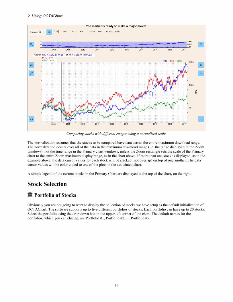
Comparing stocks with different ranges using a normalized scale.
The normalization assumes that the stocks to be compared have data across the entire maximum download range. The normalization occurs over all of the data in the maximum download range (i.e. the range displayed in the Zoom windows), not the time range in the Primary chart windows, unless the Zoom rectangle sets the scale of the Primary chart to the entire Zoom maximum display range, as in the chart above. If more than one stock is displayed, as in theexample above, the data cursor values for each stock will be stacked (not overlap) on top of one another. The data cursor values will be color coded to one of the plots in the associated chart.
A simple legend of the current stocks in the Primary Chart are displayed at the top of the chart, on the right.
Stock Selection
Portfolio of Stocks
Obviously you are not going to want to display the collection of stocks we have setup as the default initialization of QCTAChart. The software supports up to five different portfolios of stocks. Each portfolio can have up to 20 stocks.Select the portfolio using the drop down box in the upper left corner of the chart. The default names for the portfolios, which you can change, are Portfolio #1, Portfolio #2, … Portfolio #5.
18

Technical Analysis Charting for Stocks - QCTAChart
Select the current portfolio
Once the portfolio is selected, the stock symbols in the portfolio display to the right. Select the symbol in order toedit the stocks in the current portfolio.
Edit the stock list in the current portfolio
Enter valid ticker symbols for the stocks you in the portfolio in the edit box in the middle. If a ticker symbol is invalid, or is not on the list of tickers symbols supported by this software, it will be deleted when you close the dialog.
You can change the default name for the portfolio (Portfolio #1 above) by editing it in the box under Edit Stock List.
19

2. Using QCTAChart
Stock Data Adjusted for Splits and Dividends.
Every time series of stock data comes in two forms. The first is simply the daily open-high-low-close and volume data, unadjusted for stock splits and dividends. The second form adjusts the stock data for stock splits and dividends.Most all technical chart analysis assumes that you are working with stock data that is adjusted for stock splits and dividends. This prevents huge price jumps from being displayed in the chart at the time of a stock split, and smaller price jumps at the time a dividend is paid. Use the [Use unadjusted values] checkbox to select whether or not you want adjusted (the default) or unadjusted values. This selection applies to every stock in the portfolio. When comparing the Quandl-sourced download values against download values from other sources, often the source of any differences is whether or not adjusted, or unadjusted values are used.
20

3. Define the Primary Chart
Primary Chart Stocks
The Primary Chart displays a plot of one to three stocks in one of several different formats: simple line plot, OHLC plot, Candlestick plot, Mountain Plot, OHLC Bar plot, Candlestick-Volume Candlestick plot. The y-axis can be configured for a simple linear scale, a normalized linear scale, and a logarithmic scale. The user can set the maximum download range for historical stock values as 3, 10 or 30 years. Also, a single stock can be displayed as a Point and Figure plot, or a Renko plot.
The Primary Chart setup dialog is invoked using the button. The setup dialog for the primary chart lookslike:
The Primary chart dialog is invoked when you select the button
The First, Second and Third plots can represent any stock in the current portfolio. They specify how to display the stock data: a line plot, scatter plot, bar plot, mountain plot, OHLC plot, candlestick plot, candlestick volume plot. The First plot can also display the stock data as a Renko, or a Point and Figure plots. When either of these last two plot types are specified, the Second and Third plots are disabled, because the other plot types do not really mix with the scaling system used by the Renko and Point and Figure plots.
Stock Index – The primary plot item in the chart, selected from the available stocks in the current
21

3. Define the Primary Chart
portfolio.
Plot Type – The plot type for the first plot – Line, OHLC, OHLC Bar, Candlestick, Candlestick Volume, Mountain,Point and Figure, or Renko
The Color button is used to change or modify the current color, line thickness and line style for the associated plot object.
The Color button, and options button, [...], are used to define the stock plot attributes
Simple Plot Attributes using the Color Button
Color – Set the attributes of the plot. For a simple color, line thickness or line style change just choose the Color button. For other plot type specific changes, choose the three dot Options button to the right of the Color button. Plot specific Options depend on the current Plot Type value. In the case of the more complexplot types, such as the Point and Figure plot, and the Renko plot, options include plot specific items such aspricing mode, box size, reversal count and other parameters. For the OHLC, Candlestick and Candlestick Volume charts there are separate buttons for upside and downside attributes.
Dialog Box for the Color Button
Color – Select the Primary color of the line or text object.Line Width – The line width in pixels of the line – use value in range of (1,2,3,4...15)Line Style – The line style of the line (Solid, Dash, Dot, DashDot, DashDotDot)
22

Technical Analysis Charting for Stocks - QCTAChart
Fill – The fill option for the object, if applicable. It is assumed that the fill color is the same as the main, primary color, though it may have a alpha value, which makes it lighter in color and transparent. The Fill option may or may not be present, depending on the plot type, and whether or not is supports a Fill, or not Filled option.Alpha – The transparency of the line – use value in the range (0..255)
Classic Open-high-low-close plot
The classic OHLC chart used in technical analysis. Data can be zoomed and panned using the upper zoom window.
The OHLC plot type displays stock market data in an open-high-low-close format common in financial technical analysis. Every event item of the plot is a vertical line, representing High and Low values, with two small horizontal"flags", one left and one right extending from the vertical High-Low line and representing the Open and Close values. It is most useful when used to display data consisting of 10 to 50 events. Otherwise the vertical lines get too close together and it degenerates into a big smear with most of the information content lost.
If you select the options button for the OHLC plot, […], you will see the Upside and Downside buttons for OHLC plot.
Select the options button and then use the Upside and Downside buttons to set the colors of the OHLC plot
Upside Color – The color attributes for the plot object when the close is higher than the open
23

3. Define the Primary Chart
Downside Color – The color attributes for the plot object when the open is higher than the close
Candlestick Plot
The classic Candlestick chart used in technical analysis, where the candlestick is filled if the close for that time period is lower than the open.
The candlestick plot displays stock market data in an open-high-low-close format common in financial technical analysis. Every item of the plot is represented by a vertical line representing High and Low values, overlapped by a box representing the Open and Close values. If the Close value is greater than the Open value for a particular candlestick, the box is filled, otherwise it is unfilled. Like the OHLC plot, the candlestick plot is best used when there are between 10 and 50 event items in the current time frame, else the details of the candlesticks will be too small to see.
If you select the options button for the Candlestick plot, […], you will see the Upside and Downside buttons for Candlestick plot.
24

Technical Analysis Charting for Stocks - QCTAChart
Candlestick-Volume plot
The Candlestick-Volume plot is a Candlestick plot which uses a variable width for the candlestick box. The item width is set proportional to the volume for that time period, adding another dimension to the chart.
There is a variant of the Candlestick plot called the Candlestick-Volume plot. The variant is that relative volume information for each candlestick is encoded in the candlestick width. We do not implement the traditional Candlestick-Volume, because it uses a very irregular x-axis which will not sync up with our other technical indicator plots. Instead, we look at the data in the current view of the chart, and assign the maximum candlestick width to the maximum Volume value (from the OHLCV data) in the current view. That volume is assigned a width of 1.0, and all other candlesticks are assigned widths less than one, equal to the ratio of Volume/(Maximum Volume). When you look at a Candlestick-Volume plot, you will immediately see which candlesticks occurred on days with the highest volume, since they will be the widest. In the example above, the day with the highest volume are 10/13/2014. If you plot an actual volume plot underneath, you can see the relationship between candlestick width, and volume.
25

3. Define the Primary Chart
In the picture above, the fattest candlestick items correspond to the time periods where the trading volume was the highest.
If you select the options button for the Candlestick-Volume plot, […], you will see the Upside and Downside buttons for Candlestick-Volume plot.
26

Technical Analysis Charting for Stocks - QCTAChart
Simple line plot of close values
When you have more then 50 or so data items, it is best to use the line plot type to display closing values.
When you compare two or three stock, using a normalize y-axis scale, it is best to use the line plot type.
27

3. Define the Primary Chart
When you compare two or more stocks of different ranges, use the Normalized y-scale. It normalizes the compared stocks to 0% at the beginning of the full-range time frame. In the example above, the blue line represents the normalized stock price of Apple, which increased 200% to 300% more than its peers. Use the Y-Scale option of the Primary Chart setup dialog to switch over to normalized stock prices.
When you compare two or three stock of different price ranges, it is best to use a normalize y-scale.
28

Technical Analysis Charting for Stocks - QCTAChart
Mountain (or filled) close plot
A filled version of the line plot is called a Mountain plot.
A Mountain plot is just a line plot, with the area under the line filled down to the x-axis. You set the color of the Mountain plot using the Color button. The color sets the upper-most line color, while the fill area is set to a transparent variant of the selected color.
Bar plot
The Bar plot uses solid colored bars to plot the closing stock price.
Similar to the simple Line plot, the Bar plot plots a bar from the x-axis up to the stock value. You set the color of theBar plot using the Color button. Best used for 50 data points or less, otherwise the bars are squeezed together and the space between the bars will start to disappear.
29

3. Define the Primary Chart
Scatter plot
The Scatter plot plots a symbol at the closing stock price.
Similar to the simple Line plot, the Scatter plot plots a symbol at the stock value. You set the color of the Scatter plot using the Color button. Best used for 50 data points or less, since adjacent symbols are close in value and start to overlap. You can set properties such as symbol type, symbol size, and symbol fill, using the options button, [...].
Where the Scatter plot setup options are:
Color – Primary color of the scatter plot objectSymbol – The symbol used in the scatter plot (Square, Up Triangle, Down Triangle, Diamond, Cross, Plus,Star, Line, Hbar, Vbar, and Circle)Fill – fill the symbolSymbol Size (Pts) – Size of the scatter plot symbol in points
30

Technical Analysis Charting for Stocks - QCTAChart
Point and Figure Charts
Point and Figure charts do not plot price against time as other techniques do. Instead it plots price against changesin direction by plotting a column of Xs as the price rises and a column of Os as the price falls.
Point and Figure plots have been used in technical analysis for more than 100 years. It is unique in that it does not plot price against time as other techniques do. Instead it plots price against changes in direction by plotting a columnof Xs as the price rises and a column of Os as the price falls. As long the stock price is increasing, and does not backtrack by more than a multiple (usually 3) of the box size, the price increase is displayed as an increasing vertical column of Xs, one X for each time the stock price breaks through the top of a box price level. Once the trend reverses more than a multiple of the box value, the column increments to the right, and changes over to a column of 0's, which are plotted down as long as the stock price continues to drop, without any significant reversals.Many technicians like it because it filters out much of the normal up and down noise in the stock data, and makes it very easy to identify trends up or down. As in the example above, it compresses the time frame, so that many years of data (eight+ in the example above) can be displayed without crowding.
A good book on the subject is Point and Figure Charting by Thomas J. Dorsey. More detailed description of our Point and Figure chart implementation is found in Chapter 7 of this manual, Point and Figure Charts.
If you select the options button for the Point and Figure plot, […], you will see color and setup parameter options for the chart.
31

3. Define the Primary Chart
Setup options for the Point and Figure plot
Where the Point and Figure setup options are:
Box Size Mode – Specifies the box size calculation mode used in calculating the Box size for the Point andFigure chart – Traditional, Percentage or Fixed, or Fixed ATR.Box Size – The fixed box size used in calculting and drawing the Point and Figure chart.Pricing Mode – Selects if the High/Low method or the Close method is used in the Point and Figure chart calculation.Reversal Count – Specifies the fixed reversal count used in the Point and Figure chart calculationsUpside - Color used for text or boxes in an up-trend.Downside – Color used for text or boxes in an down-trend.
32

Technical Analysis Charting for Stocks - QCTAChart
Renko Charts
Renko charts do not plot price against time as other techniques do. Instead it plots price against changes in direction by unfilled boxes as the price rises and filled boxes as the price falls.
Renko charts are similar to Point and Figure charts, in that they do not plot price against time as other techniques do.Instead it plots price against changes in direction by plotting unfilled boxes (called bricks in Renko terminology) as the price rises and filled boxes as the price falls. As long the stock price is increasing, and does not backtrack by more than the brick size size, the price increase is displayed as an rising diagonal of bricks. Each time the price rises enough to warrant a new brick, a new column is started and the brick is plotted in that column. Once the trend reverses, as each new brick is added on the downside, a new column is started. No column will every contain more than one brick. The result is a chart similar to the example above, where time scales are irregular and compressed. The net result is a strong filtering of the OHLC data, eliminating the ever present noise present in market data.
More detailed description of our Renko chart implementation is found in Chapter 8 of this manual, Renko Charts.
If you select the options button for the Renko plot, […], you will see color and setup parameter options for the chart.
33

3. Define the Primary Chart
Setup options for the Renko plot
Where the Renko setup options are:
Box Size Mode – The box size mode – either Fixed or Fixed ATR.Box Size – The fixed box size used in calculting and drawing the Renko chart.Pricing Mode – Selects if the High/Low method, Close or Typcial Price price method is used in the Renko chart calculation.ATR Period – Specifies the period in days used in the ATR pricing mode calcultion.Upside - Color used for boxes in an up-trend.Downside – Color used for boxes in an down-trend.
34

4. Technical Indicator overlays for the Primary chart
Primary Chart Technical Indicators
The Primary chart can also have technical indicators over-laid on top of the stock data. This includes:
Simple moving averages
Exponential moving averages
Moving Average Bands
Bollinger Bands
Parabolic SAR
Select the button to setup the Primary Chart technical indicators dialog.
Simple moving averagesSimple moving averages (SMA) are a easy way to filter out random noise, or price fluctuations, from a signal. Filtering makes it easier to identify short and long term trends in stock movement. A single simple moving average (MA) is often compared to original signal. When the original signal passes up and through the SMA, that can be considered a buy signal.
It is often considered a buy signal when the stock prices breaks through the 50 day moving average.
35

4. Technical Indicator overlays for the Primary chart
It is considered a buy signal when the blue OHLC data passes up and through the 50 point SMA above. The opposite is also true; it is considered a sell signal if the signal drops below the SMA.
Often times two or more moving averages of different lengths, acting on the same underlying signal, are compared and conclusions made based on intersection points between the SMA signals. If the shorter of two SMA signals passes up and through the longer, it is considered a buy signal. If the shorter of the two SMA signals passed down and through the longer, it is considered a sell signal.
It is often considered a buy signal if a short term simple moving average passes up and through a long term moving average.
In the picture above, the red line is a 15 point moving average, and the green line is a 50 point moving average. When the 15 point moving average pass up and through the 50 point moving average, that is considered a buy signal.
A SMA signal is simple to calculate. It is the unweighted mean of the previous n data items. The N period SMA for a time series Y(t) it can be calculated using the formulas
Starting with i = N (the SMA signal starts at the Nth data point)
i = N
SMA[i] = (Y[i] + Y[i-1] + Y[i-2] . . . Y[i-N+1]) / N
When calculating successive values, a new value comes into the sum and an old value drops out, meaning a full summation each time is unnecessary for this simple case,
i > N
SMA[i] = SMA[i-1] - Y[i-N] / N + Y[i] / N
36

Technical Analysis Charting for Stocks - QCTAChart
The setup for the simple moving average is accessed by selecting the button.
Calculatate and plot as an overlay of the stock plot, one or two simple moving averages of the first plotted dataset.
Where:
Moving Average #1First – Enable the first simple moving averagePeriod – The period of the first moving average.Color – Set the color attributes of the plot
Moving Average #2First – Enable the second simple moving averagePeriod – The period of the second moving average.Color – Set the color attributes of the plot
Exponential moving averagesThe disadvantage of simple moving averages (SMA) is that it gives equal weight to all event items. If you are using a 200 period SMA, then the oldest data point 200 days ago is given the same weight in the calculation as the most recent. Most practitioners of technical analysis are going to want more recent data values to have a greater influence on the indicator than older values.
The exponential moving average (EMA) mathematically weights more recent data more than older data. Because of this it can react quicker to changing circumstances. Otherwise, the buy and sell rules are much the same as the SMA.If the shorter of the EMA signals moves up and through the longer, it considered a buy signal. If the shorter of the EMA signals moves down and through the longer, it considered a sell signal. It can be used singly or in pairs, same as the SMA examples.
37

4. Technical Indicator overlays for the Primary chart
Many traders prefer the exponential moving average (EMA) over the simple moving average (SMA), because the EMA weighs more recent data more heavily than old data.
A EMA signal is simple to calculate. The EMA for a time series Y(t) it can be calculated using the formula:
Starting with i = N (the EMA signal starts at the Nth data point), the first value is calculated as the simple moving average (SMA) of the same time period. This gives a starting point for the EMA calculation.
i = N
EMA[i] = SMA[i]
Subsequent calculations use the formula.
i > N
EMA[i] = EMA[i-1] * (1 – alpha) + Y[i] * alpha
where EMA[i] is the current EMA value
EMA[i-1] is the previous EMA value
alpha is the smoothing constant in the range 0.0 to 1.0
Y[i] is the current value of the source signal
In words, the EMA calculation is the current value of the source signal (the stock closing price), multiplied by the alpha value, plus the previous value of the EMA calculation, multiplied by (1 – alpha). The net effect is a weighted moving average where the older the source signal value is, the less it contributes to the current EMA value.
For a given signal, the only unknown in the equation above is the smoothing constant alpha. Financial technicians use a simple formula to calculate this value. If you specify a N point EMA, this implies that the alpha value is equal to 2 / (N + 1). For example, a 50 period EMA is equal to 2 / (50 + 1) = 0.0392 . Specifying a 50 period EMA is the
38

Technical Analysis Charting for Stocks - QCTAChart
same as specifying a 0.0392 alpha value for the EMA calculation. You won't see the alpha value referenced anywhere else. We will stick with the standard way to define a financial, technical analysis, EMA, which is to say that it is a N-point EMA.
The setup for the exponential moving average is accessed by selecting the button.
Calculatate and plot as an overlay of the stock plot, one or two exponential moving averages of the first plotteddataset.
Where:
Moving Average #1First – Enable the first exponential moving averagePeriod – The period of the first exponential moving average.Color – Set the color attributes of the plot
Moving Average #2Second– Enable the second exponential moving averagePeriod - The period of the second exponential moving average.Color – Set the color attributes of the plot
Moving Average BandsMoving Average Bands (or Envelopes) are formed by calculating a SMA (usually a 20-period average) on a source signal, and then forming two bands above and below the SMA signal by adding and subtracting a percentage deviation (usually in the range 1% to 10%) from the SMA signal. Moving average bands serve as an indicator of overbought or oversold conditions, visual representations of price trend, and an indicator of price breakouts.
39

4. Technical Indicator overlays for the Primary chart
Traders look for when the stock price breaks out of the moving average bands.
Trading Strategies Moving Average Bands
When the stock price does not appear to be trending up or down:
Buy when the Low of the OHLC stock price penetrates the lower envelope and closes back inside the envelope.
Sell when the stock price High of the OHLC price penetrates the upper envelope and then closes back down inside the envelope.
When the stock price breaks out above or below the envelop – trending one direction or the other:
Buy when the prices break above the upper envelope
Sell when prices break below the lower envelope
Moving Average Band Formulas
Moving average bands are simple to calculate. Start with a SMA of the signal (usually the Close value of the OHLC)and a bandwidth of BW. The two bands are:
for all i
UpperBand[i] = SMA[i] * (1 + BW)
LowerBand[i] = SMA[i] * (1 – BW)
40

Technical Analysis Charting for Stocks - QCTAChart
The setup for the Moving Average Bands is accessed by selecting the button. You may have to scroll vertically toget to this section.
This section of the dialog shows both MA Bands and Bollinger Bands options
Where:
Enable – Enable the Moving Average Bands plotPeriod – The period of the moving average used in the Moving Average Bands smoothingBandwidth % – The bandwidth, as a percentage of the moving average value of the source signalColor – Set the color attributes of the plot.Fill – Set the fill between the band lines. Off by default for MA Bands.
Bollinger BandsBollinger Bands (or Envelopes) are similar to Moving Average bands, except they add a little statistical science to the formation of the indicator. Bollinger Bands still use a SMA calculation for the central line (20 period SMA is standard). But instead of using a fixed percentage as the band width, it defines the separation between the two bandsusing a multiple of the standard deviation signal, calculated using the previous N periods of the closing value of the OHLC data. The theory is that stock price action follows a normal distribution about the mean, and 95% of a stocks price movement should fall within two standard deviations, plus and minus, of the mean value. Price action outside of the +-2 standard deviations band signifies that something unusual happening and that you expect some sort of break in the current trend.
41

4. Technical Indicator overlays for the Primary chart
Traders look for when the stock price breaks out of the Bollinger bands (much the same as Moving Average bands).
The filled area represents the Bollinger bands. Usually Bollinger bands include the SMA line, orange in this case.
Trading Strategies Bollinger
Interpretations of Bollinger Bands vary, but one is that when stock prices push up and through the upper band, the stocks are thought to be overbought. And when stock prices push down through the lower limit, stocks are thought to be oversold. Therefore:
Sell when the stock prices push upward through the upper limit.
Buy when the stock prices push downward through the lower limit.
There are entire books written about Bollinger Band trading strategies, including one by John Bollinger, "Bollinger on Bollinger Bands", the man who invented the indicator. So don't expect their practical use to be as cut and dry as the buy/sell signals described above.
Bollinger Band Formulas
K = Standard deviation multiple - usually equal to 2
for all i
SD = Standard Deviation of the previous N (usually 20) values in the N period SMA
UpperBand[i] = SMA[i] * (1 + K * SD)
LowerBand[i] = SMA[i] * (1 – K * SD)
42

Technical Analysis Charting for Stocks - QCTAChart
The setup for Bollinger Bands is accessed by selecting the button. You may have to scroll the dialog to get to the Bollinger Bands setup.
This section of the dialog shows both MA Bands and Bollinger Bands options
Where:
Enable – Enable the Bollinger Bands plotPeriod – The period of the moving average used in the Bollinger Bands smoothingBandwidth (SD) – The bandwidth, in Standard Deviations, of the Bollinger Bands plotColor – Set the color attributes of the plot.Fill – Check and the area between the Bollinger Bands is filled with a trasparent color. On by default for Bollinger Bands
Parabolic SAR
The Parabolic SAR is used by traders to set stop loss orders for a stock.
In the example above, the green dots represent the Parabolic SAR indicator
43

4. Technical Indicator overlays for the Primary chart
The Parabolic SAR (Parabolic Stop and Reverse) is probably the strangest looking indicator. The Parabolic in the name comes from the accelerating rise and fall of the indicator around the source signal.
The well known market technician J. Welles Wilder created the indicator and described it in his book New Concepts in Technical Trading Systems. Published in 1978, the book also describes a number of other Welles indicators, including the Average True Range, the Directional Movement Index and the Relative Strength Index.
When the parabola is below the price action it is considered bullish, and when i it is above the price action, it is considered bearish. Since it forecasts one day in advance, traders often use the Parabolic SAR value to set stop limitsfor trades that day. For example, in an upward trend, if the stock price falls below the P SAR value for that day, sell the stock in order to protect gains.
Parabolic SAR Formulas
PSARn (Parabolic Stop And Reverse) = today’s value of the Parabolic SAR
PSARn+1 = Tomorrow's value for the PSAR. The PSAR formula forecasts one day in advance
EP (Extreme Point) = The highest high of the current uptrend or the lowest low of the current downtrend.
AF (Acceleration Factor) = Determines the sensitivity of the PSAR. AF starts at .02 and increases by .02 every time the EP rises in a Rising PSAR or EP falls in a Falling PSAR. The maximum value is usually clamped at 0.20. The starting value, 0.02, step value 0.02 and maximum value 0.20, are all variables in the software and you can choose anything you want.
PSARn+1 = PSARn + AFn*(EPn - PSARn)
where
AF is calculated according to the rules described above.
Special conditions which override the calculated value
If in an upward trend, the new PSAR value is calculated and if the result is more than today’s or yesterday’s lowest price, it must be set equal to the lower of those two days. Some texts (not Wilder's) say to set it to the closer of the two lows. We use the lower of the two lows in this software.
In a downward trend the new PSAR value is calculated and if the result is less than today’s or yesterday’s highest high price, it must be set equal to the higher of those two days. Some texts (not Wilder's) say to set it to the closer of the two highs. We use the higher of the two highs in this software.
If the next period’s PSAR value is inside (or beyond) the next period’s price range, a new trend direction is then signaled. The PSAR must then switch sides.
Upon a trend switch, the first PSAR value for this new trend is set to the last EP recorded on the prior samedirection trend, EP is then reset accordingly to this period’s maximum, and the acceleration factor is reset to its initial value of 0.02. On re-calculation of the new SAR after the switch, some packages will check to see if the new EP changes (rises in an uptrend or falls in a down trend) first, and boost the acceleration factor on the first calculation, making it 0.04. We always force the first calculation after a switch-over to use an acceleration factor of 0.02, and on subsequent calculations within the trend we increase it a step at a time as the EP changes.
The setup for PSAR is accessed by selecting the button. You may have to scroll the dialog to get to the PSAR
44

Technical Analysis Charting for Stocks - QCTAChart
setup.
Where:
Enable – Enable the Parabolic SAR plotStart Index – starting index value for the Parabolic SAR plotStep Start – the starting step size for the for the Parabolic SAR plotStep Increment – The size of the increment to the step step size when it changesStep Max – The maximum allowable value of the step sizeColor – Set the color attributes of the plot.
45

5. Secondary Chart Indicators
Secondary Chart Technical Indicators
Underneath the primary chart you can display additional, technical indicator, charts. The secondary charts are used to display technical indicators which are best displayed in their own chart area, usually because they use a y-axis coordinate system which is not the same as the primary chart. The secondary charts always key on the first stock in the primary chart, so you cannot monitor one stock in the Primary chart (INTC for example) and another in the secondary charts (TXN for example).
Many of the secondary chart technical indicators display multiple lines, or bar plots, as part of their display. Also, many use explicit alarm limits to notify the user that a buy or sell signal is taking place.
Below is a current list of the secondary indicators available for display in the software.
Average Directional Indicator
Momentum
Rate of Change (ROC)
Relative Strength (RSI)
Stochastic (Fast and Slow)
Williams %R
Moving Average Convergence/Divergence (MACD)
Volume charts
Adding Secondary Charts (Technical Indicators)The Secondary charts setup dialog is accessed by selecting the button.
47

5. Secondary Chart Indicators
The Secondary chart technical indicators are accessed by scrolling vertically in the dialog.
Volume Indicators
Traders expect that major changes in the direction of a trend are accompanied by high volume.
48

Technical Analysis Charting for Stocks - QCTAChart
Volume represents the number of shares, or contracts, which traded during a period of time. Since it is part of the standard OHLCV price packet available in historical data feeds, it gives valuable information about the significanceof the price action of a stock. A price movement in either direction is considered more relevant if is is simultaneous with a large increase in share volume. If you are monitoring the trend of a stock, and that stock suddenly reverses the trend, that is the time to check the volume to see if the reversal was accompanied by a sharp increase in the trading volume. If not, then that can be a sign that there is no conviction by the trend reversal, and you can expect the stock to reverse back. Volume charts can be smoothed using the standard smoothing techniques to help filter out the noise of no use to the trader.
Trading Strategies Volume
Buy when
Buy when the trend moves from negative to positive, if the transition is accompanied by large volume.
Sell when
Sell when the trend moves from positive to negative, if the transition is accompanied by large volume.
The setup for the Volume indicator is accessed by selecting the button. Add a Volume indicator to the chart by selecting Enable in the Volume setup.
Where:
Volume – Enable a Volume bar plotVolume and MA – Enable a Volume bar plot with a moving average line plot of volumePeriod – The period of the moving averageSmoothing – The moving average type: Specify Simple moving average, exponential moving average, or Wilder exponential moving averageVolume – Color attributes for the Volume barsMoving Average – Color attributes for the Volume moving average line
Money Flow (MFI)The Money Flow indicator is considered an oscillator, cycling between 0 and 100. it was create by market technicians Gene Quong and Avrum Soudack. It uses both the Typical Prices for a period, and the period volume, inits calculation. It is sometimes referred to as a volume adjusted RSI indicator.
49

5. Secondary Chart Indicators
The Money Flow indicator provides more information than the Relative Strength indicator, because it also takes into account volume.
Trading Strategies Money Flow
Action LimitsSet high (overbought) and low (oversold) thresholds for action limits. Recommended value for the high limit is 80, and the low limit is 20.
Buy whenThe Money Flow indicator drops below the lower threshold and then rises back above it.
A reverse of the indicator to the upside while the overall stock trend is down. The money flow reversal is considered a leading indicator of the future stock trend.
Sell whenThe Money Flow indicator crosses to above the overbought level and then falls back below it.
A reverse of the indicator to the downside while the overall stock trend is up. The money flow reversal is considereda leading indicator of the future stock trend.
Formula
Calculate the Typical Price for each period = (High + Low + Close)/3
Calculate the Raw Money Flow for each period = Typical Price x Volume
For each period, calculate as separate values the positive money flow over the previous N periods (usually 14), and the negative money flow over the same time frame.
Calculate the Money Flow Ratio as the ratio (Positive Money Flow)/(Negative Money Flow)
50

Technical Analysis Charting for Stocks - QCTAChart
Normalize Money flow ratio for the range 0-100 using:
Money Flow Index = 100 - 100/(1 + Money Flow Ratio)
The setup for the Money Flow indicator is accessed by selecting the button. Add a Money Flow indicator to the chart by selecting Enable in the Money Flow setup.
Where:
Enable – Enable the Money Flow Indicator chartPeriod– The period used in the Money Flow calculationLimits– Display limits in the chartColor – The color attributes of the Money Flow indicator.
Limit Attributes – Many of the secondary chart indicators have limits associated with them. At the very bottom of the dialog, the Misc. Items section of the dialog will set the limit attributes
51

5. Secondary Chart Indicators
Relative Strength (RSI)
The Relative String Indicator compares the magnitude of gains (up-Closes) versus losses (down-Closes) for the timeperiod under consideration, in order to determine when a stock is overbought or oversold.
The Relative Strength Indicator (RSI) was originally developed by J. Welles Wilder and is described in his book "New Concepts in Technical Trading System". It indicates strength or weakness in a security based on the closing price action within the specified trading period. The RSI is calculated using the ratio of higher closes to lower closes: stocks which have had more or stronger positive changes have a higher RSI than stocks which have had moreor stronger negative changes. The RSI indicator is normalized so all values are percentages in the range 0 to 100. Intermediate values in the calculation are smoothed using the Wilder exponential smoothing method, usually using a14 day period.
Trading Strategies RSI
Action LimitsRecommended action limits for RSI are a high limit of 70, and a low limit of 30.
In a non-trending market
Buy when
Buy when the RSI value passes upwards and through the low action limit (30).
Sell when
Sell when the RSI value passes downward and through the high action limit (70).
In a trending market
52

Technical Analysis Charting for Stocks - QCTAChart
Buy when
Buy when the RSI value passes upwards and through the low action limit (40).
Sell when
Sell when the RSI value passes downward and through the high action limit (60).
Formula
For i >= 1
if (Close [i] - Close [i-1]) > 0
U[i] = (Close [i] - Close [i-1])
D[i] = 0;
else if (Close [i-1] - Close [i]) > 0
U[i] = 0
D[i] = (Close [i-1] - Close [i])
else if (Close [i-1] - Close [i]) == 0
U[i] = 0
D[i] = 0
Each U[i] and D[i] value is smoothed using an N period exponential smoothing routine. The result is
U[i]Sm
D[i]Sm
The RS value is calculated as
RS[i] = U[i]Sm / D[i]Sm
and finally, the RSI values is normalized to the range 0 to 100 using the formula
RSI[i] = 100 – (100 / (1 + RS[i]))
The setup for the RSI indicator is accessed by selecting the button. You may have to scroll the dialog vertically to get to this option. Add an RSI indicator to the chart by selecting Enable in the RSI setup.
53

5. Secondary Chart Indicators
Where:
Enable – Enable the RSI Indicator chartPeriod– The period used in the RSI calculationLimits– Display limits in the chartColor – Color attributes for the RSI indicator line
Limit Attributes – Many of the secondary chart indicators have limits associated with them. At the very bottom of the dialog, the Misc. Items section of the dialog will set the limit attributes
Williams %R
The Williams %R indicator is used to detect overbought and oversold conditions for the given stock.
Williams %R was developed by Larry Williams, a publisher of trading and technical analysis materials, to indicate overbought and oversold market conditions for a stock. Similar to the Stochastic indicator, it compares a stock's close to the high-low range over a certain period of time, usually 14 days. For some strange reason the indicator is normalized in the range 0.0 to -100, so that an overbought condition is represented by the indicator above the -20 line, and an oversold condition represented by the indicator below -80. A value of -100 for the index means that the close today was at the lowest low of the past N days, and a value of 0 for the index means that a close today was at the highest high of the past N days. When it is plotted the Williams %R indicator looks the same as the Stochastic %K indicator, except that the y-axis values are shifted down by 100.
54

Technical Analysis Charting for Stocks - QCTAChart
Trading Strategies Stochastic
Action LimitsRecommended action limits for Williams %R charts, are a high limit of -20 (overbought), and a low limit of -80 (oversold). While Williams himself specifies a 10 day period, most users prefer the 14 day period, the same as the Stochastic %K indicator.
Williams used a 10 trading day period and considered values below -80 as oversold and above -20 as overbought. Most users seem to use a 14 day period though, consistent with the Stochastic indicator time period.
Buy when
Buy when the %R line passes down and through the low (-80) action limit value.
Sell when
Sell when the %R line passes up and through the high (-20) action limit value.
Formulas
The Williams %R indicator is calculated as:
%R[i] = -100 * ((Close[i] – H14[i])/(H14[i] – L14[i]))
where Close[i] is the periods closing price, L14[i] is the lowest low for the last N periods, and H14[i] is the highest high for the last N periods, where N is usually 14 periods. This results in a value of -100 to 0. A %R[i] value of over -20 means that the closing price is very near the top of the OHLC range, and a value of under -80 means that the closing price is near the bottom of the OHLC range.
The setup for the Williams %R indicator is accessed by selecting the button. You may have to scroll the dialog vertically to get to this option. Add an Williams %R indicator to the chart by selecting Enable in the Williams %R setup.
Where:
Enable – Enable the Williams (%R) indicator chartPeriod– The period used in the Williams (%R) calculationLimits– Display limits in the chartColor – Set the color attributes of the indicator line
Limit Attributes – Many of the secondary chart indicators have limits associated with them. At the very bottom of the dialog, the Misc. Items section of the dialog will set the limit attributes
55

5. Secondary Chart Indicators
Rate of Change (ROC)The Rate of Change indicator is essentially a normalized version of the Momentum indicator. It takes the Momentum value at each time period and divides it by the Close price N days ago, where N is the same value used in the Momentum calculation. The result is multiplied by 100 to convert from a fraction to a percentage.
The bottom chart is the Rate of Change indicator, which is a normalized version of the Momentum indicator.
Trading Strategies Rate of Change
Buy when
When in an up trend, buy when the ROC value passes upward through zero.
Sell when
When in a down trend sell when the ROC value passes downward through zero
Formula
For i >= N
ROC[i] = 100 * ((Close [i] - Close [i-N])/ Close [i-N])
56

Technical Analysis Charting for Stocks - QCTAChart
The setup for the Rate of Change indicator is accessed by selecting the button. You may have to scroll the dialogvertically to get to this option. Add an Rate of Change indicator to the chart by selecting Enable in the Rate of Change setup.
Where:
Enable – Enable the Rate of Change indicator chartPeriod– The period used in the Rate of Change calculationColor – The color attributes of the Rate of Change line
Momentum (also known as the Change Indicator)The Momentum indicator is used to identify the speed (or strength) of a price movement. It is calculated as the difference between today's closing price and the close N days ago.
While the Momentum indicator is positive, it designates an continuing upward trend in prices. A negative upward trend designates a continuing downward trend.
57

5. Secondary Chart Indicators
Trading Strategies Momentum
Action LimitsSet high (overbought) and low (oversold) thresholds for action. No firm algorithm is available for this. Some suggest setting the thresholds at 67% the high and low peak values on both sides of 0.0.
Buy when The Momentum indicator drops below the lower threshold and then rises back above it
Sell when Momentum crosses to above the overbought level and then falls back below it. On a bearish divergence - with the first peak above the overbought level.
Formula
For i >= N
Momentum[i] = (Close [i] - Close [i-N])
The setup for the Momentum indicator is accessed by selecting the button. You may have to scroll the dialog vertically to get to this option. Add an Momentum indicator to the chart by selecting Enable in the Momentum setup.
Where:
Enable – Enable the Momentum indicator chartPeriod– The period used in the Momentum calculationLimits– Display limits in the chartColor – The color attributes of the Momentum line
Limit Attributes – Many of the secondary chart indicators have limits associated with them. At the very bottom of the dialog, the Misc. Items section of the dialog will set the limit attributes
58

Technical Analysis Charting for Stocks - QCTAChart
Stochastic (Fast and Slow)
The bottom chart plots %K vs %D Fast Stochastic
The Stochastic indicator was developed by George Lane, president of Investment Educators Inc, Watseka, IL. It is based on the assumption that as prices trend upwards, closing prices tend to be in the upper part of the periods OHLC price range. And the opposite is true, in down trends, closing prices tend to be in the lower part of the periodsOHLC price range.
Formulas
The first line in the Stochastic indicator is the %K line. The %K line is calculated as
%K[i] = 100 * ((Close[i] – L14[i])/(H14[i] – L14[i]))
where Close[i] is the periods closing price, L14[i] is the lowest low for the last Nk periods, and H14[i] is the highesthigh for the last Nk periods, where Nk is usually 14 periods. This results in a value of 0 to 100. A %K[i] value of over 80 means that the closing price is very near the top of the OHLC range, and a value of under 20 means that the closing price is near the bottom of the OHLC range.
The second line in the Stochastic indicator is the %D line. The %D line is calculated as a simple Nd point moving average of the %K line, where Nd is usually 3 periods. So it is just a slower, smoother version of %K line. The 3 period smoothed version of %D is known as the Fast Stochastic indicator. If %D is smoothed using a 3 period average, then it becomes the Slow Stochastic indicator. The Slow Stochastic indicator is the more widely used. One confusing item is that both the Fast Stochastic and the Slow Stochastic are referred to as %D.
59

5. Secondary Chart Indicators
The bottom chart plots %K vs %D Slow Stochastic. If you compare it to the previous chart you will see that the red line is more smoothed, and lags a bit.
Trading Strategies Stochastic
Action LimitsRecommended action limits for Stochastic charts are a high limit of 80, and a low limit of 20.
Buy when
Buy when the %K line passes up and through the %D line when the %D line is below the low (20) action limit value.
Sell when
Sell when the %K line passes down and through the %D line when the %D line is above the high (80) action limit value.
The setup for the Stochastic indicator is accessed by selecting the button. You may have to scroll the dialog vertically to get to this option. Add an Stochastic indicator to the chart by selecting Enable in the Stochastic setup.
60

Technical Analysis Charting for Stocks - QCTAChart
Where:
Period – The period used in the Stochastic %K calculation
Fast (%D) – Enable the display of the Fast Stochastic line plotPeriod - The period of the Fast Stochastic calculation
Slow (%D) – Enable the display of the Slow Stochastic line plotPeriod - The period of the Slow Stochastic calculation
Limits– Display limits in the chart
Stoch. %K – Color attributes for the %K lineFast %D – Color attributes for the Fast %D lineSlow %D – Color attributes for the Slow %D line
Limit Attributes – Many of the secondary chart indicators have limits associated with them. At the very bottom of the dialog, the Misc. Items section of the dialog will set the limit attributes
61

5. Secondary Chart Indicators
Moving Average Convergence/Divergence (MACD)
MACD is used as a measure of the strength, direction, momentum and length of a trend.
The MACD was developed by Gerald Appel and is discussed in his book, The Moving Average Convergence Divergence Trading Method. It is a comparison of several moving averages (exponential) derived from a stocks closing prices.
The first EMA uses a 26 day period and is referred to as the long EMA line. The second EMA uses a 12 day periodand is referred to as the short EMA line. The MACD line is calculated by subtracting the long (26) EMA line from the short (12) EMA line. The signal line is calculated as a 9 day EMA of the MACD line. The two lines actually plotted in the indicator are the MACD line, and the signal line. The crossover of MACD and signal lines indicates a buying or selling opportunity. Additionally, a histogram, representing the differences between the MACD line, and the signal line, is usually part of a MACD chart.
Trading Strategies Stochastic
Buy when
Buy when the MACD line passes up and through the signal line - this corresponds to the histogram going positive.
Sell when
Sell when the MACD line falls below the signal line – this corresponds to the histogram going negative.
Formulas
62

Technical Analysis Charting for Stocks - QCTAChart
The MACD indicator is calculated as follows:
The long EMA line is calculated as the EMA(nlong) of the close prices.
The short EMA line is calculated as the EMA(nshort) of the close prices.
The MACD line is calculated as the difference between the long EMA and the short EMA.
The signal line is calculated as the EMA(nsignal) of the MACD line.
The histogram is calculated as the MACD line minus the signal line.
Where nlong, nshort and nsignal represent the exponential smoothing periods for the long EMA, the short EMA and the signal line, respectively.
Special Note
Some packages use a SMA (Simple Moving Average), rather than an EMA (Exponential Moving Average) in the calculations. That is not how the MACD is normally defined though.
The setup for the MACD indicator is accessed by selecting the button. You may have to scroll the dialog vertically to get to this option. Add an MACD indicator to the chart by selecting Enable in the MACD setup.
Where:
Enable – Enable the MACD indicator chartFast Period – The fast period used in the MACD chartSlow Period – The slow period used in the MACD chartSignal Smoothing Period – The moving average type: Specify Simple moving average, exponential moving average, or Wilder exponential moving averageMACD Line – Color attributes for the MACD lineSignal Line – Color attributes for the Signal lineHistogram Line – Color attributes for the Histogram bars
63

5. Secondary Chart Indicators
Average Directional Indicator (ADX)
The bottom chart is the ADX indicator and it is used to measure the strength of a trend.
The Average Directional Indicator (ADX) was originally developed by J. Welles Wilder and is described in his book"New Concepts in Technical Trading System". The ADX is used to measure the strength of a trend. Its related components, the Minus Directional Indicator (-DI) and Plus Directional Indicator (+DI), are used to measure the strength of a trend. The ADX indicator is often used in conjunction with the Parabolic SAR indicator, to confirm a trend. In the chart above, the Primary chart shows the Parabolic SAR indicator, and the bottom chart shows the ADX indicator (blue line), the -DI indicator (green line) and the +DI indicator (red line);
A stock is said to be in a strong trend if the ADX value is greater than 25 (some use 20 as the threshold). Note, that the ADX indicator does NOT specify a trend direction. So a strong positive trend, or a strong negative trend, will result in ADX values greater than 25 (20). So the ADX value can signal traders whether or not they should be using trend trading strategy.
Assuming you are in an upward trend confirmed by an ADX value of 25 (or 20), a buy signal occurs when +DI crosses above – DI, with a stop loss place on the low of the day. The buy signal remains as long as this low holds, even if +DI crosses back below - DI. If the stock price falls below the stop loss low, the buy signal is ended. If the trade become profitable, traders should uses stop losses (perhaps the Parabolic SAR value) to protect their profit. A sell signal occurs when - DI crosses above +DI.
ADX, +DI and -DI Formulas
The ADX indicator is a slow moving signal, because it uses long exponential smoothing periods. Also, it uses unique variant of exponential smoothing, called Wilder smoothing. As discussed in the Exponential Moving Average section, the standard exponential smoothing equation is:
EMA[i] = EMA[i-1] * (1 – alpha) + Y[i] * alpha
alpha is the smoothing constant in the range 0.0 to 1.0
64

Technical Analysis Charting for Stocks - QCTAChart
for regular (non-Wilder) time-based exponential moving average calculations, the alpha value is calculated as:
alpha = 2 / (N + 1)
where N is the number of time periods specified in the smoothing (in a 20 point exponential smooth of a set of data, the alpha value is calculated as (2 / 21) or 0.0952. But in the case of Wilder smoothing, the formal for alpha is
alpha = 1 / N
so that if the period length is 20, the alpha value of the exponential smoothing equations becomes 0.05.
The ADX indicator also uses something called the True Range, which is a value for each period calculated from the OHLC for that period and the previous period. The formula is:
for i>0
True Range[i] = Max( Highs[i] – Lows[i], Abs(Highs[i] – Closes[i-1]), Abs(Closes[i-1] – Lows[i]))
Because the + and – signs in front of +DM and -DM can be confused with arithmetic operators, we rename those indicators pDM and mDM for remaining formulas.
for i>0
pDM[i] = Highs[i] - Highs[i-1] Positive in a rising trendmDM[i] = Lows[i-1] - Lows[i] Positive in a falling trend
An inside day (where both calculations are negative) both values are set to 0.
If pDM[i] >= mDM, then pDM[i] remains at its calculated value, mDM[i] is set to 0.0.
If pDM[i] < mDM, then mDM[i] remains at its calculated value, mDM[i] is set to 0.0.
Calculate the True Range values for the OHLC data
TR14 = 14 period Wilder EMA of True Range data
Calculate the 14 Period Wilder EMA of the pDM and mDM data
pDM14 = 14 period Wilder EMA of pDM data
mDM14 = 14 period Wilder EMA of mDM data
Calculate the +DI and -DI indicators
for i > 0
65

5. Secondary Chart Indicators
pDI14[i] = pDM14[i] divided by TR14[i]
mDI14[i] = mDM14[i] divided by TR14[i]
Then, calculate the components of the Average Directional Movement Index (ADX):
ADX[i] = 100 * ABS((pDI14[i] - mDI14[i]) / (pDI14[i] + mDI14[i]))
ADX14 = 14 period Wilder EMA of ADX
The actual returned values are the pDI14 array, the mDI14 array and the ADX14 array, all representing 14 period Wilder EMA of the underlying index.
Special Note
The proper use of the ADX indicator always requires that your historical data start at least 150 periods (days) prior to the time period you are interested in. Because it takes that long for the exponential smoothing averages to settle down. Results where your data starts only 50 days before the the time period you are interested will be similar to, but not the same as the results where a 150 day lead time is used.
The setup for the ADX indicator is accessed by selecting the button. You may have to scroll the dialog verticallyto get to this option. Add an ADX indicator to the chart by selecting Enable in the ADX setup.
Where:
Enable – Enable the ADX indicator chartPeriod – The fast period used in the ADX chartSmoothing – The moving average type: Specify Simple moving average, exponential moving average, or Wilder exponential moving averageLimits– Display limits in the chartADX Line – Color attributes for the ADX lineDM+ Line – Color attributes for the DM+ lineDM- Line – Color attributes for the DM- line
66

Technical Analysis Charting for Stocks - QCTAChart
6. Technical Analysis Drawing Objects
Primary Chart Drawing Tools
There is a small set of technical analysis objects which can be placed in the Primary chart. These are trend lines , a financial Fibonacci object, horizontal and vertical data markers, arrows, and two types of labels for annotations. Thefirst label type, called Text, is positioned using normalized coordinates, and does not scroll when the chart scrolls. The second label type, called Label, is tied to specific time coordinates and will scroll when the chart is scrolled.
The technical analysis drawing objects are accessed using the Drawing Tool button, , on the left side of the chart. Select that button and you will see a toolbar of drawing objects.
Use the Drawing button, , to invoke the drawing toolbar
67

6. Technical Analysis Drawing Objects
Trend Line
Drawing a trend line helps determine support and resistance levels for a stock trending upwards or downwards.
Start by selecting the Drawing Tool button, , on the left side of the chart. Then select Trend. Click (touch) the startand ending point of the trend line in the Primary Chart window. This is two separate clicks (touches), not a click anddrag operation. The trend line can be moved by click (touch)-dragging the center of the line. The slope of the line is controlled by click (touch)-dragging the endpoints of the trend line. The price values of the trend line endpoints are also displayed. Once placed, you can still adjust the position of the line with great precision.
You can edit the trend line properties by selecting it be clicking (touching) it once. Then select the Drawing button, then select Edit from the resulting toolbar. That will invoke the trend line edit dialog, seen below.
You can customize the look of the trend line using the Trend Line Dialog
68

Technical Analysis Charting for Stocks - QCTAChart
Options for the Trend Line Dialog
Line AttributesColor – Primary color for the objectLine Width – The line width in pixels of the line – use value in range of (1,2,3,4...15)Line Style – The line style of the line (Solid, Dash, Dot, DashDot, DashDotDot)Show Handles – Check and the grab handles of the trend line are displayed at the endpoints.
Text Attributes
Numeric precision – Set the numeric precision of the numeric labels at the line endpoints.Font – Edit the text Font and Font Size
Text Color – Select the color of the textBackground – Select the background color of the textUse Background – Check this box if you want the background rectangle of the text to overwrite what is underneath.Plot Area Clipping – Check this box if you want the text to clip to the plotting area (the area bounded by the axes)Horizontal Justify – Sets horizontal text justification of the trend line start label. The justificationof the trend line end label is set to the opposite value.Vertical Justify – Sets vertical text justification of the trend line start label. The justification of the trend line end label is set to the opposite value.
Horizontal and Vertical data markers
The horizontal data marker is useful for marking support and resistance levels.
69

6. Technical Analysis Drawing Objects
Start by selecting the Drawing Tool button, , on the left side of the chart. Select HLine, click on the chart at the desired location, and a horizontal data marker will appear. It can be moved in a vertical plane. The y-value of the marker is displayed on the left. Once placed, you can still adjust the position of the line with great precision.
You can edit the HLine properties by selecting it be clicking (touching) it once. Then select the Drawing button, , then select Edit from the resulting toolbar. That will invoke the HLine edit dialog, which is the same as the Trend line dialog discussed in the previous section.
A vertical data marker is useful for making important time period.
Similarly, the VLine option from the Drawing toolbar will place a vertical data marker on the chart, which can be moved in the horizontal plane. The date of the marker is displayed at the top. It can be edited the same way as the HLine marker.
Fibonacci Overlay
A Fibonacci overlay is used to predict support and resistance levels for a stock.
A Fibonacci overlay is used in some types of technical analysis wave theory to identify support and resistance levelsfor a stock. The values on the right of the horizontal lines in the example above (0, 23.6, 38.2, 50.0, 61.8, 100, 161.8 and 261.8) represent percentage values and are calculated using the famous Fibonacci sequence (0, 1, 1, 2, 3, 5, 8, 13, 21, 34, 55, 89, 144, 233). How do the first set of values derive from the second you ask?
Choose a seed value from the Fibonacci sequence of 89.
233/89 = 2.618
70

Technical Analysis Charting for Stocks - QCTAChart
144/89 = 1.618
89/89 = 1.00
55/89 = 0.618
34/89 = 0.382
21/89 = 0.236
And the 0.50 level is thrown in for good measure, because market technicians like 50% as a retracement level.
Typically you place the bottom of the Fibonacci rectangle at a local minimum, and the maximum at a local maximum, and the intermediate values represent price support and resistance levels.
Select the Fibon option from the Drawing toolbar, then click (touch) the lower-left corner, and the upper-right corner, of where you want the Fibonacci overlay. The Fibonacci overlay will be drawn at the selected location, with the Fibonacci levels 0 and 100 at the click points. The overlay can be adjusted by click (touch)-dragging the corners,or the center, of the overlay. If you define the Fibonacci rectangle by clicking (touching) the top corner point first, then the bottom corner point, an inverted Fibonacci sequence will be created, with the 0.0 level at the top, and levelsincreasing towards 262, downward.
You can edit the Fibonacci properties by selecting it be clicking (touching) it once. Then select the Drawing button, , then select Edit from the resulting toolbar. That will invoke the Fibonacci edit dialog, seen below.
Attribute options for the Fibonacci Dialog
71

6. Technical Analysis Drawing Objects
Line AttributesColor – Primary color for the objectLine Width – The line width in pixels of the line – use value in range of (1,2,3,4...15)Line Style – The line style of the line (Solid, Dash, Dot, DashDot, DashDotDot)Show Handles – Check and the grab handles of the trend line are displayed at the endpoints.
Text AttributesNumeric precision – Set the numeric precision of the numeric labels at the line endpoints.Font – Edit the text Font and Font Size
Text Color – Select the color of the textBackground – Select the background color of the textUse Background – Check this box if you want the background rectangle of the text to overwrite what is underneath.Plot Area Clipping – Check this box if you want the text to clip to the plotting area (the area bounded by the axes)Horizontal Justify – Sets horizontal text justification of the trend line start label. The justificationof the trend line end label is set to the opposite value.Vertical Justify – Sets vertical text justification of the trend line start label. The justification of the trend line end label is set to the opposite value.
Labels for Annotation
Text objects do not scroll with the chart x-axis, and are used for text that you always want on the chart, regardless of the time frame.
There are two types of labels you can use for annotations. The first is a Text object. It is placed in the chart using Normalized graph coordinates. Because of this, it does not scroll, or change position, when the graph y-scale is changed, or when the graph is panned or zoomed. Because Normalized Graph coordinates do not change even if the
72

Technical Analysis Charting for Stocks - QCTAChart
graphs physical coordinate system changes.
The Label object will scroll with the chart.
The second type of annotation is the Label. It is placed in the chart using Physical graph coordinates. Because of this, it scrolls, and change position, when the graph y-scale is changed, or when the graph is panned or zoomed. Because the Label object sticks to the physical coordinates where it was placed.
Select the Text or Label option from the Drawing toolbar, then click the position where you want the label. You willthen see a dialog box with options regarding font, the text string, colors, and justification. When you close the dialog, the label will be drawn at the click location. The overlay can be adjusted by click (touch)-dragging the center of the label.
Unlike the Text objects, Label objects do scroll when the x-axis scrolls, and are used when you want the label to track the underlying plot.
73

6. Technical Analysis Drawing Objects
The Edit Text dialog will appear when you first click (press) the position of the text, and also if you select Edit for that object from the Drawing toolbar
Attribute options for the Text and Label Dialog
Font – Edit the text Font and Font SizeText – The text string to display as a labelForeground Color – Select the color of the textBackground Color – Select the background color of the textUse Background – Check this box if you want the background rectangle of the text to overwrite what is underneath.Plot Area Clipping – Check this box if you want the text to clip to the plotting area (the area bounded by the axes)Horizontal Justify – Sets horizontal text justification of the numeric label. Vertical Justify – Sets vertical text justification of the numeric label.
All you really need to do is enter the string you want displayed. But you can change the other default values if you need to. The text string will appear at the selected xy-position.
Text and Label objects can be moved into position by left-click (touch)-dragging anywhere on the text.
The Text object does not change position, even if the graph scaling changes.
Arrows for Annotation
74

Technical Analysis Charting for Stocks - QCTAChart
Arrow objects include a text annotation (similar to a Label object). Arrow objects will scroll with the data.
The Arrow object is a line, ending in an arrowhead at one end, and annotation at the other, which can be place in theprimary chart. The line placement and slope, the arrowhead size, the line width, text and font are all user programmable.
Select the Arrow option from the toolbar, then click the starting (the arrow head), and ending position where you want the arrow. You will then see a dialog box with options regarding Font, the text string, colors, justification, andarrowhead size. When you close the dialog, the arrow, and accompanying label will be drawn using the starting and ending click locations. The arrow can be adjusted by click-dragging the endpoints, or the shaft of the arrow.
Use the Arrow object to highlight areas of the chart. Start by selecting the Drawing Tool button, , on the left side of the chart. Then select Arrow. Click (touch) the start (the arrow tail) and ending (arrowhead) point of the arrow in the Primary Chart window. This is two separate clicks (touches), not a click and drag operation. At the end of the second click (touch) a Edit Arrow dialog will appear so that you can enter the arrow text.
The arrow can be moved by click (touch)-dragging the center of the line. The slope of the line is controlled by click (touch)-dragging the endpoints of the arrow line. Once placed, you can still adjust the position of the line with greatprecision.
75

6. Technical Analysis Drawing Objects
You can edit the arrow properties by selecting it be clicking (touching) it once. Then select the Drawing button, thenselect Edit from the resulting toolbar. That will invoke the arrow edit dialog, seen above.
Arrow Attributes
Line Color – Primary color for the objectWidth – The line width in pixels of the line – use value in range of (1,2,3,4...15)Size – The size of the arrowhead in pointsShow Handles – Check and the grab handles of the trend line are displayed at the endpoints.
Text Attributes
Text – The text string to display as a labelFont – Edit the text Font and Font SizeForeground Color – Select the color of the textBackground Color – Select the background color of the textUse Background – Check this box if you want the background rectangle of the text to overwrite what is underneath.Plot Area Clipping – Check this box if you want the text to clip to the plotting area (the area bounded by the axes)Auto Justify Text – Sets horizontal and vertical text justification of the numeric label depending on the angle of rotation of the arrowHorizontal Justify – Sets horizontal text justification of the numeric label. Vertical Justify – Sets vertical text justification of the numeric label.
76

7. Point and Figure Charts
Point and Figure charts have been used to analyze the stocks and the market for more than 100 years
Point and Figure plots have been used in technical analysis for more than 100 years. A P&F chart is unusual in that it does not plot price against time as other techniques do. Instead it plots price against changes in direction. It does so by plotting a column of Xs as the price rises and a column of Os as the pricefalls. As long the stock price is increasing, and does not backtrack by more than a multiple (usually 3) of the box size, the price increase is displayed as an increasing vertical column of Xs, one X for each time thestock price breaks through the top of a box price level. Once the trend reverses more than a multiple of the box value, the column increments to the right, and changes over to a column of 0's, which are plotted down as long as the stock price continues to drop, without any significant reversals. Electrical and control systems engineers will recognize this as a programmable form of hysteresis. Many technicians like it because it filters out much of the normal up and down noise in the stock data, and makes it very easy to identify trends up or down. As in the example above, it compresses the time frame, so that many years of data (seven in the example above) can be displayed without crowding.
A good book on the subject is Point and Figure Charting by Thomas J. Dorsey.
Our version of the Point and Figure charts includes most of the features found in advanced versions. It marks the years of the columns along the x-axis. Months are indicated in-column using numbers 1 to 9 and letters A, B, and C as most implementations do.
The Point and Figure chart type can be set using First Plot combo boxes of the Primary Chart Dialog page. Only the First Plot has the Point and Figure option. When it is set to Point and Figure, the chart types for the Second Plot and Third Plot are ignored.
77

7. Point and Figure Charts
Point and Figure y-Axis Scale ModesThere are four common methods used to scale the y-axis: traditional, percentage, fixed, and fixed ATR. The traditional mode is the most common. The traditional y-axis scale described above,with changes in box size at values of 1, 5, 20, 100..., is generally meant for a stock price range of 5 to 100. It uses mostly integer based numericvalues because these are easier to calculate and plot by hand – a legacy of the 100 year history of point and figure charts. But many stocks have a much broader range, especially in non-US markets where the valuation of the stocks in the local currency can be in the thousands. In these cases, a percentage based method is preferrable. When the percentage method is used, each box size is a fixed percentage larger than the preceding box size. The two fixed modes ( fixed, and fixed ATR) are useful if the stocks are moving in a relatively narrow range, overlapping one of thetraditional mode break-points (1, 5, 20, 100, 200, etc.), and you want to force a constant fixed box size to keep the box size from changing at the breakpoints.
Traditional Box Size
The box-size for the y-axis is increases as the price increase, even within the same column, and follows the traditional box size convention:
Price Box size
0.0 to <=0.25 0.0625
>0.25 to <=1 0.125
>1 to <=5 0.25
>5 to <=20 0.5
>20 to <=100 1.0
>100 to <=200 2.0
>200 to <=500 4.0
>500 to <=1000 5.0
>1000 to <=25000 50.0
> 25000 500.0
In the traditional scaling mode, we use these breakpoints, even though they do not look symetrical across decade ranges.
Under Price, the range is exclusive of the first value and inclusive of the second value. So the second range is actually 0.26 to 1.0, and the third range is actually 1.01 to 5.0, and so on.
78

Technical Analysis Charting for Stocks - QCTAChart
Point and Figure chart of Intel over ten years, using the traditional box size mode
If you look at the y-axis tick marks in the chart above, you will notice that the in the range of 12 to 20, the box size, represented by the tick spacing, is 0.5. Once the values reach a range greater than 20, the box size shifts to 1.0. This is in accordance with the Price / Box Size table above. If the prices in the chart increased above 100, the box size would change to 2.0.
Percentage Box Size
In the percentage method is used, each box size is a fixed percentage larger than the preceding box size. In the chart below, the P&F chart above has been recast using a percentage y-scale.
79

7. Point and Figure Charts
Point and Figure chart of Intel over ten years using the percentage box size mode. A percentage value of 4% was used in this case
Note that the box size, and hence the tick mark spacing, increases by a fixed percentage (4% in this case), from the starting, or minimum y-axis value. This permits charts with a wide dynamic range (Apple for example) to be plotted,keeping the same relative resolution at the minimum and maximum values of the chart.
Fixed Box Size
Another method is to just force the chart to your own choice of a fixed box size. In the example below the chart is recast using a fixed box size of 1. The box size can be a whole number (1,2,3,4...) or a fraction (0.5, 0.75, 1.33...)
80

Technical Analysis Charting for Stocks - QCTAChart
Point and Figure chart of Intel over ten years using the fixed box size mode. A box size of 1 was used in this case.
Fixed Box Size using ATR (Average True Range)
The fixed box size has the drawback in that it is not auto-ranging. A stock where the values in the time frame of interest are in the hundreds (IBM or Apple) will need a much larger fixed box size, than other stocks with values in the teens. The traditional and percentage methods take this into account with their non-linear scales. A variant of the fixed box size mode calculates fixed box size as a function of the Average True Range, where the Average True Range (defined by J. Welles Wilder) is defined as below.
The true range for a given time period is maximum of several calculated ranges:
True Range = Max ( Current High less the current Low,
Abs(Current High - previous Close ),
Abs(Current Low - previous Close ) )
The Average True Range is a moving average (14-day Moving Average in this case) of the most recent and previous13 values. The fixed box size is set to the value of the Average True Range calculated using the most recent data. Below is the P&F chart we have been using as an example, configured for a fixed box size calculated using the Average True Range.
81

7. Point and Figure Charts
In this example, the Average True Range is used to calculated the box size.
In this case the fixed box size was calculated to be approximately 0.5.
Point And Figure Setup OptionsFirst use select the Primary Chart dialog using the buton. Set the plot type for the First Plot to Point & Figure.
The Point & Figure options can be set using the First Plot options button, [...], found there. The options are then added to the dialog immediately below the First, Second and Third Plot setup section.
82

Technical Analysis Charting for Stocks - QCTAChart
Box Size Mode
The Box Size Mode combo box is used to select the P&F box size mode: Traditional, Percentage, Fixed, or ATR.
Box Size
If you select a Box Size Mode of Fixed, or Percentage, the box size is set to the value of the Box Size field. If you select a Box Size Mode of Percentage, then the percentage used in the calculation is the value of Box Size convertedto percent. For example, a Box Size of 1 represents 1 percent (0.01). A value of 0.5 represents 0.5 percent (0.005). Ifyou select a box Size of Fixed, the box size is set to the value of Box size.
If you select Traditional or ATR, the Box Size field is ignored.
ATR Period
If the Box Size Mode is set to Fixed ATR, the ATR look-back period is specified using the ATR Period combo box, seen below.
83

7. Point and Figure Charts
Pricing Mode
The price input to the chart takes one of three forms. You can plot the chart using Close prices only. Or you can use the most popular method which uses the days High and Low values. The third method is similar to the first option, but instead of using the Close price, the Typical Price is used, where the Typical price is defined as: (High value + Low value + Close value) / 3.
Set the Pricing Mode combo box to the value you want.
High Low Method
Here is the basic psuedo-code algorithm for the High-Low method.
IF (you are currently in an X-column, i.e. prices have been rising)
{
IF (High breaks out of the current box into a new, higher box)
draw the new X and ignore the Low
ELSE IF (Low triggers a 3-box reversal)
Start a new column and fill in Os down to to current Low
ELSE
Do nothing
}
ELSE IF (you are currently in an O-column, i.e. prices have been falling)
{
IF (Low breaks out of the current box into a new, lower box)
draw the new O 's
ELSE IF (High triggers a 3-box reversal)
Start a new column and fill in Xs up to to current High
84

Technical Analysis Charting for Stocks - QCTAChart
ELSE
Do nothing
}
Close Method
Here is the basic psuedo-code algorithm for the Close method
IF (you are currently in an X-column, i.e. prices have been rising)
{
IF (Close breaks out of the current box into a new, higher box)
draw the new X
ELSE IF ( Close triggers a 3-box reversal)
Start a new column and fill in Os down to to current Close
ELSE
Do nothing
}
ELSE IF (you are currently in an O-column, i.e. prices have been falling)
{
IF ( Close breaks out of the current box into a new, lower box)
draw the new O 's
ELSE IF ( Close triggers a 3-box reversal)
Start a new column and fill in Xs up to to current Close
ELSE
Do nothing
}
Typical Price Method
The Typical Price for each OHLC event is calculated as: (High value + Low value + Close value) / 3.
Here is the basic psuedo-code algorithm for the Typical Price method
IF (you are currently in an X-column, i.e. prices have been rising)
{
85

7. Point and Figure Charts
IF ( Typical Price breaks out of the current box into a new, higher box)
draw the new X
ELSE IF ( Typical Price triggers a 3-box reversal)
Start a new column and fill in Os down to to current Typical Price
ELSE
Do nothing
}
ELSE IF (you are currently in an O-column, i.e. prices have been falling)
{
IF ( Typical Price breaks out of the current box into a new, lower box)
draw the new O 's
ELSE IF ( Typical Price triggers a 3-box reversal)
Start a new column and fill in Xs up to to current Typical Price
ELSE
Do nothing
}
Reversal Count
The reversal count is the number of boxes the price of a stock must change, in order to trigger a P&F reversal. A reversal is when the chart transitions from Xs and Os, (and vise-versa), and a new column is started in the chart. Typically this value is three, but it can be anything from 1 to N.
The reversal count is set using the Reversal Count field.
Color Options
Select the Upside and/or Downside Attributes buttons to change the Point and Figure colors.
86

Technical Analysis Charting for Stocks - QCTAChart
Select the Upside or Downside color and the stanard color chooser dialog will appear.
87

8. Renko Charts
Renko charts do not plot price against time as other techniques do. Instead it plots price against changes indirection by plotting unfilled boxes as the price rises and a filled boxes as the price falls.
Renko charts are similar to Point and Figure charts, in that they do not plot price against time as other techniques do. Instead it plots price against changes in direction by plotting filled boxes (called bricks in Renko terminology) as the price rises and unfilled boxes as the price falls. As long the stock price is increasing, and does not backtrack by more than the brick size size, the price increase is displayed as an rising diagonal of bricks. Each time the price rises enough to warrant a new brick, a new column is started and the brick is plotted in that column. Once the trend reverses, as each new brick is added on the downside, a new column is started. No column will every contain more than one brick. The result is a chart similar to the example above, where time scales are irregular and compressed. The net result is a strong filtering of the OHLC data, eliminating the ever present noise present in market data.
Renko y-Axis Scale ModesUnlike Point and Figure charts, which in the Traditional and Percentage scale modes use a non-linear y-axis, Renko charts always use a linear y-axis scale. Also, Renko charts always use a fixed box size. The box size can be set by the user, or it can be automatically calculated using the ATR for a given look-back period.
Fixed Box Size
The user has the option of specifying a fixed box sise. In the example below the chart is recast using a fixedbox size of 2. The box size can be a whole number (1,2,3,4...) or a fraction (0.5, 0.75, 1.33...)
89

8. Renko Charts
Renko chart for TXN over ten years using fixed box size of 2
Fixed Box Size using ATR (Average True Range)
The fixed box size has the drawback in that it is not auto-ranging. A stock where the values in the time frame of interest are in the hundreds (IBM or Apple) will need a much larger fixed box size, than other stocks with values in the teens. A variant of the fixed box size mode calculates fixed box size as a function of the Average True Range, where the Average True Range (defined by J. Welles Wilder) is defined as below.
The true range for a given time period is maximum of several calculated ranges:
True Range = Max ( Current High less the current Low,
Abs(Current High - previous Close ),
Abs(Current Low - previous Close ) )
The Average True Range is a moving average (14-day Moving Average in this case) of the most recent and previous13 values. The fixed box size is set to the value of the Average True Range calculated using the most recent data. Below is the Renko chart we have been using as an example, configured for a fixed box size calculated using the Average True Range.
90

Technical Analysis Charting for Stocks - QCTAChart
The Average True Range can be used to automatically calculate the box size.
In this case the fixed box size was calculated to be approximately 0.8.
Renko Chart Setup OptionsFirst use select the Primary Chart dialog using the buton. Set the plot type for the First Plot to Renko.
The box size mode can be set using the First Plot options button, [...] found there. The options are then added to the dialog immediately below the First, Second and Third Plot setup section.
91
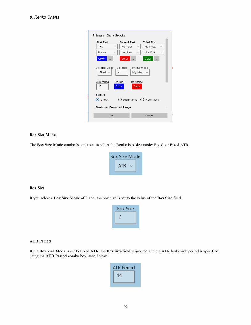
8. Renko Charts
Box Size Mode
The Box Size Mode combo box is used to select the Renko box size mode: Fixed, or Fixed ATR.
Box Size
If you select a Box Size Mode of Fixed, the box size is set to the value of the Box Size field.
ATR Period
If the Box Size Mode is set to Fixed ATR, the Box Size field is ignored and the ATR look-back period is specified using the ATR Period combo box, seen below.
92

Technical Analysis Charting for Stocks - QCTAChart
Renko Price Mode
The price input to the chart takes one of three forms. You can plot the chart using Close prices only. Or you can usethe most popular method which uses the days High and Low values. The third method is similar to the first option, but instead of using the Close price, the Typical Price is used, where the Typical price is defined as: (High value + Low value + Close value) / 3.
Set the Pricing Mode combo box to the value you want.
High-Low Method
Here is the basic algorithm for the High-Low method.
IF (High breaks out of the current box into a new, higher box)
Advance one column and draw the new box using the upside color and ignore the Low
ELSE (Low breaks out of the current box into a new, lower box)
Advance one column and draw the new box using the downside color
ELSE
Do nothing
The High-Low method produces more fluctuations in the resulting chart than the Close method.
Close Method
Here is the basic algorithm for the Close method
IF ( Close breaks out of the current box into a new, higher box)
Advance one column and draw the new box using the upside color
ELSE ( Close breaks out of the current box into a new, lower box)
Advance one column and draw the new box using the downside color
ELSE
Do nothing
Typical Price Method
93

8. Renko Charts
The Typical Price for each OHLC event is calculated as: (High value + Low value + Close value) / 3.
IF ( Typical Price breaks out of the current box into a new, higher box)
Advance one column and draw the new box using the upside color
ELSE ( Typical Price breaks out of the current box into a new, lower box)
Advance one column and draw the new box using the downside color
ELSE
Do nothing
Color Options
Select the Upside and/or Downside Attributes buttons to change the Point and Figure colors.
Select the Upside or Downside color and the stanard color chooser dialog will appear. Check the Fill option if you want the Renko bricks filled.
94

9. Miscellaneous Setup Items
General Chart Setup
This setup dialog allows the user to specify options controlling the overall look of the chart display. The user can specify the colors used in the chart, along with line widths, the text sizes and the overall text font. An option is included to use the European convention for dates (dd/mm/yy), then than the default US convention (mm/dd/yy).
The General chart setup dialog is accessed by selecting the button.
Misc. Colors
Button – set the color of the buttons placed around the edge of the chartZoom Area – Set the color of the zoom rectangleTitle – Set the color of the chart titleStocks – Set the color of the stock symbols listed across the top of the screen
95

9. Miscellaneous Setup Items
Chart Area Background
Style – Set the background style for the overall chart area – solid or vertical gradient.Color #1 – Set the color for the solid background color style. Also the first color used if the gradient background style is selected.Color #2 – Set the color for the second color used in the gradient background color style.
Plot Area Background
Style – Set the background style for the plotting ares of the chart – solid or vertical gradient.Color #1 – Set the color for the solid background color style. Also the first color used if the gradient background style is selected.Color #2 – Set the color for the second color used in the gradient background color style.
X-Axes
Line – Use the standard color chooser dialog to set the line color, and thickness of the axis.Text – Use the standard color chooser dialog to set the color of the axis labels.
Y-Axes
96
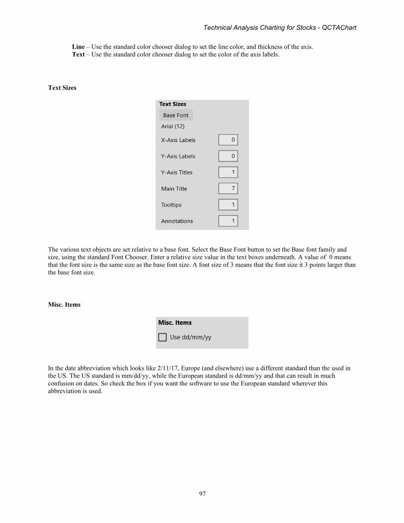
Technical Analysis Charting for Stocks - QCTAChart
Line – Use the standard color chooser dialog to set the line color, and thickness of the axis.Text – Use the standard color chooser dialog to set the color of the axis labels.
Text Sizes
The various text objects are set relative to a base font. Select the Base Font button to set the Base font family and size, using the standard Font Chooser. Enter a relative size value in the text boxes underneath. A value of 0 means that the font size is the same size as the base font size. A font size of 3 means that the font size it 3 points larger thanthe base font size.
Misc. Items
In the date abbreviation which looks like 2/11/17, Europe (and elsewhere) use a different standard than the used in the US. The US standard is mm/dd/yy, while the European standard is dd/mm/yy and that can result in much confusion on dates. So check the box if you want the software to use the European standard wherever this abbreviation is used.
97

Technical Analysis Charting for Stocks - QCTAChart
10. File and Printer Rendering
Printing - Print the current chart to an available printer.
Saving Image to a File - Save an image of the chart to local storage.
Printing a Chart
Select the Printer option, , in the bottom left of the application if you want to print the current chart. The standard Windows App printer dialog, with a couple of additions, will appear. Adjust the settings to your liking.
We added Centering Mode and Size Mode options to the standard printer dialog. That way you center the chart horizontally, vertically, both, or neither.
99

10. File and Printer Rendering
The Size Mode option supports an automatic maximize scaling, explicit scaling, and unscaled (actual size).
If the Scaled option is selected, a scaling factor can be entered.
The charts aspect ratio (W/H) cannot be changed, meaning that the scale factor for the x-dimension and the y-dimension will always be the same.
Capturing the Chart as an ImageSelect the Printer option, , in the leftmost toolbar of the application if you want to save the current chart as an image file to local storage on your device. The standard Windows App Save As file dialog will appear.
100

Technical Analysis Charting for Stocks - QCTAChart
Use the Save As file dialog to specify the image file location, name and output type.
Select the file location, file name and output type of your image file. Supported output types include JPEG, TIF, GIF, BMP, and PNG.
101

Technical Analysis Charting for Stocks - QCTAChart
Index
Alphabetical IndexArrows...............................................................................................................................................................................................
Arrows...................................................................................................................................................3, iv, 5, 67, 75Average Directional Indicator............................................................................................................................................................
Average Directional Indicator...................................................................................................................3, iv, 47, 64Average True Range..........................................................................................................................................................................
Average True Range........................................................................................................................44, 81, 82, 90, 91Bollinger Bands.................................................................................................................................................................................
Bollinger Bands....................................................................................................................3, iv, 5, 7, 35, 41, 42, 43Box Size Mode..................................................................................................................................................................................
Box Size Mode.........................................................................................................32, 34, 79, 80, 81, 83, 90, 91, 92Candlestick........................................................................................................................................................................................
Candlestick..............................................................................................................1, 2, iv, 5, 7, 9, 21, 22, 24, 25, 26Candlestick-Volume.................................................................................................................................................25Candlestick, Candlestick..........................................................................................................................................22
ChartPrint..........................................................................................................................................................................................Printing.....................................................................................................................................................................99
Classic Open-high-low-close.............................................................................................................................................................Classic Open-high-low-close..........................................................................................................................2, iv, 23
Customer Support..............................................................................................................................................................................customer support...................................................................................................................................................iv, 6
data cursors........................................................................................................................................................................................data m...................................................................................................................................................................3, 67data markers.............................................................................................................................................................69
Dimension..........................................................................................................................................................................................dimension...............................................................................................................................................................100
Equi-volume candlestick plot.............................................................................................................................................................Candlestick-Volume Candlestick plot..................................................................................................................2, 21Candlestick-Volume plot.........................................................................................................................................25
event-based coordinate system...........................................................................................................................................................event-based coordinate system.............................................................................................................................iv, 9
Exponential moving averages............................................................................................................................................................exponential moving averages..............................................................................................................3, iv, 35, 37, 39Volume.....................................................................................................................................................................49 37, 39
Fibonacci overlay...............................................................................................................................................................................Fibonacci overlay......................................................................................................................................3, iv, 70, 71
Financial Chart objects......................................................................................................................................................................Financial Chart objects...............................................................................................................................................3
Financial Data Sources......................................................................................................................................................................Financial Data Sources...............................................................................................................................................4
FinText.............................................................................................................................................................................................. 72
Fixed Box Size...................................................................................................................................................................................fixed box size...........................................................................................................32, 34, 78, 80, 81, 82, 89, 90, 91
Fixed Box Size using ATR (Average True Range)............................................................................................................................Fixed Box Size using ATR (Average True Range)...........................................................................................81, 90
Free Data Sources..............................................................................................................................................................................free data sources.........................................................................................................................................................4
Google Finance..................................................................................................................................................................................Google Finance......................................................................................................................................................4, 5Google Finance (now discontinued)..........................................................................................................................5
High-Low Method.............................................................................................................................................................................High-Low method..............................................................................................................................................84, 93
103
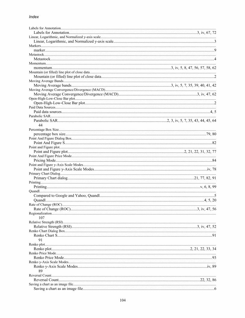
Index
Labels for Annotation........................................................................................................................................................................Labels for Annotation...............................................................................................................................3, iv, 67, 72
Linear, Logarithmic, and Normalized y-axis scale.............................................................................................................................Linear, Logarithmic, and Normalized y-axis scale....................................................................................................3
Markers..............................................................................................................................................................................................marker........................................................................................................................................................................9
Metastock..........................................................................................................................................................................................Metastock...................................................................................................................................................................4
Momentum.........................................................................................................................................................................................momentum......................................................................................................................3, iv, 5, 8, 47, 56, 57, 58, 62
Mountain (or filled) line plot of close data.........................................................................................................................................Mountain (or filled) line plot of close data................................................................................................................2
Moving Average Bands.....................................................................................................................................................................Moving Average bands...................................................................................................3, iv, 5, 7, 35, 39, 40, 41, 42
Moving Average Convergence/Divergence (MACD)........................................................................................................................Moving Average Convergence/Divergence (MACD)..............................................................................3, iv, 47, 62
Open-High-Low-Close Bar plot.........................................................................................................................................................Open-High-Low-Close Bar plot.................................................................................................................................2
Paid Data Sources..............................................................................................................................................................................Paid data sources....................................................................................................................................................4, 5
Parabolic SAR...................................................................................................................................................................................Parabolic SAR.............................................................................................................2, 3, iv, 5, 7, 35, 43, 44, 45, 64 44
Percentage Box Size..........................................................................................................................................................................percentage box size............................................................................................................................................79, 80
Point And Figure Dialog Box............................................................................................................................................................Point And Figure S...................................................................................................................................................82
Point and Figure plot..........................................................................................................................................................................Point and Figure plot....................................................................................................................2, 21, 22, 31, 32, 77
Point And Figure Price Mode............................................................................................................................................................Pricing Mode............................................................................................................................................................84
Point and Figure y-Axis Scale Modes................................................................................................................................................Point and Figure y-Axis Scale Modes................................................................................................................iv, 78
Primary Chart Dialog.........................................................................................................................................................................Primary Chart dialog..............................................................................................................................21, 77, 82, 91
Printing..............................................................................................................................................................................................Printing.........................................................................................................................................................v, 6, 8, 99
Quandl...............................................................................................................................................................................................Compared to Google and Yahoo, Quandl..................................................................................................................5Quandl..............................................................................................................................................................4, 5, 20
Rate of Change (ROC).......................................................................................................................................................................Rate of Change (ROC)..............................................................................................................................3, iv, 47, 56
Regionalization.................................................................................................................................................................................. 107
Relative Strength (RSI)......................................................................................................................................................................Relative Strength (RSI).............................................................................................................................3, iv, 47, 52
Renko Chart Dialog Box....................................................................................................................................................................Renko Chart S..........................................................................................................................................................91 91
Renko plot.........................................................................................................................................................................................Renko plot..........................................................................................................................................2, 21, 22, 33, 34
Renko Price Mode.............................................................................................................................................................................Renko Price Mode....................................................................................................................................................93
Renko y-Axis Scale Modes................................................................................................................................................................Renko y-Axis Scale Modes.................................................................................................................................iv, 89 89
Reversal Count...................................................................................................................................................................................Reversal Count.............................................................................................................................................22, 32, 86
Saving a chart as an image file...........................................................................................................................................................Saving a chart as an image file...................................................................................................................................6
104

Technical Analysis Charting for Stocks - QCTAChart
Simple line plot of close data.............................................................................................................................................................Simple line plot, scatter plot or bar plot of close data................................................................................................2
Simple moving averages....................................................................................................................................................................simple moving averages............................................................................................................................3, iv, 35, 37 35, 39 moving averages.....................................................................................................................................................39
Stochastic (Fast and Slow).................................................................................................................................................................Stochastic (Fast and Slow)........................................................................................................................3, iv, 47, 59 59
Synchronize scrolling (panning)........................................................................................................................................................Synchronize scrolling (panning)................................................................................................................................3
Traditional Box Size..........................................................................................................................................................................traditional box size.............................................................................................................................................78, 79
Trend lines.........................................................................................................................................................................................trend lines.........................................................................................................................................................3, 5, 67
True Range........................................................................................................................................................................................True Range.................................................................................................................................44, 65, 81, 82, 90, 91
Typical Price Method.........................................................................................................................................................................Typical Price Method.........................................................................................................................................85, 93
Volume charts....................................................................................................................................................................................Volume charts..........................................................................................................................................4, 22, 47, 49Volume I..................................................................................................................................................................48 48
Williams %R......................................................................................................................................................................................Williams %R.......................................................................................................................................3, iv, 47, 54, 55
Yahoo Finance...................................................................................................................................................................................Yahoo Finance.......................................................................................................................................................4, 5
zooming.............................................................................................................................................................................................zooming.....................................................................................................................................................3, iv, 10, 12
............................................................................................................................................................................................................................................................................................................................................................................................................
...................................................................................................................................................................................................................................................................................................................................................................................................................................................................................................................49, 51, 69, 72, 76
Data Sources..................................................................................................................................................................................... data sources...........................................................................................................................................................4, 5
" 23
105

Technical Analysis Charting for Stocks - QCTAChart
107