quantitative analysis of purposive systems: some spadework at the
TRANSCRIPT

Psychological Review1978, Vol. 85, No. 5, 417-435
Quantitative Analysis of Purposive Systems: Some Spadeworkat the Foundations of Scientific Psychology
William T. PowersNorthbrook, Illinois
The revolution in psychology that cybernetics at one time seemed to promisehas been delayed by four blunders: (a) dismissal of control theory as a meremachine analogy, (b) failure to describe control phenomena from the behavingsystem's point of view, (c) applying the general control system model with itssignals and functions improperly identified, and (d) focusing on man-machinesystems in which the "man" part is conventionally described. A general non-linear quasi-static analysis of relationships between an organism and its environ-ment shows that the classical stimulus-response, stimulus-organism-response,or antecedent-consequent analyses of behavioral organization are special cases,a far more likely case being a control system type of relationship. Even forintermittent interactions, the control system equations lead to one simple char-acterization: Control systems control what they sense, opposing disturbances asthey accomplish this end. A series of progressively more complex experimentaldemonstrations of principle illustrates both phenomena and methodology in acontrol system approach to the quantitative analysis of purposive systems, thatis, systems in which the governing principle is control of input.
This article concerns four old conceptualerrors, two mathematical tools (which in thiscontext may be new), and a series of sixquantitative experimental demonstrations ofprinciple that begin with a simple engineer-ing-psychology experiment and go well be-yond the boundaries of that subdiscipline. Myintent is to take a few steps toward a quan-titative science of purposive systems.
Qualitative arguments on the subject ofpurpose have abounded. Skinner (1972) hasexpressed one extreme view:Science . . . has simply discovered and used subtleforces which, acting upon a mechanism, give it thedirection and apparent spontaneity which make itseem alive, (p. 3)
An extreme opposite view is expressed byMaslow (1971):
Self-actualizing individuals . . . already suitablygratified in their basic needs, are now motivated inother higher ways, to be called "metamotivations."(p. 299)
Inquiries concerning this article should be sent toWilliam T. Powers, H38 Whitfield Road, North-brook, Illinois 60062.
In the middle ground are many others whohave tried to deal with inner purposes, forexample, Kelley (1968), McDougall (1931),Rosenblueth, Wiener, and Bigelow (1968),Tolman (1932), and Von Foerster, White,Peterson, and Russell (1968). I have con-tributed some arguments as well (Powers,1973; Powers, Clark, & McFarland, 1960a,1960b). Obviously, none of these arguments,which are all qualitative, has succeeded insettling the issue of inner purposes.
In the 1940s, many of us thought that themissing quantitative point of view had beendiscovered. Cybernetics: Control and Commu-nication in the Animal and the Machine(Wiener, 1948) seemed to contain the con-ceptual tools that might at last explain how"mental" causes could enter into "physical"effects. It seemed that a bridge might be builtbetween inner experiences and outer appear-ances. A cybernetic revolution in psychologyseemed just about to start. Now, in the late1970s, it is still just about to start. Some-thing happened to the original impetus ofcybernetics, as a river entering the desertsplits into a hundred wandering channels and
Copyright 1978 by the American Psychological Association, Inc. 0033-295X/78/8505-0417$00.75
417

418 WILLIAM T. POWERS
sinks into the sand. I have some suggestionsas to what went wrong.
Four Blunders
It is not so much honest labor on my partthat puts my name to this critique as it is aseries of blunders (qualitative mistakes) byothers who could have done long ago what Iam doing now. However unavoidable, theseblunders have been directly responsible for thefailure of cybernetics and related subjects toprovide new directions for psychology.
Machine Analogy Blunder
In 1960, the president of the Society ofEngineering Psychologists wrapped up theprevious decade of cybernetics as follows:
The servo-model, for example, about which therewas so much written only a decade or two ago,now appears to be headed toward its proper posi-tion as a greatly oversimplified inadequate descrip-tion of certain restricted aspects of man's behavior. . . . Whenever anyone uses the word model, I re-place it with the word analogy. (Chapanis, 1961,p. 126)
This view is still held. There are and havebeen for some time scientists who think ofcontrol system models of behavioral organiza-tion as a mere analogy of human behavior tothe behavior of a technological invention.
A little digging underneath the engineeringmodels suggests that this opinion is mistaken.Servomechanisms have always been designedto take over a kind of task that had previouslybeen done by human beings and higher ani-mals and by no other kind of natural system,that of controlling external variables (bring-ing them to predetermined states and activelymaintaining them in those states against anynormal kind of disturbance; Mayr, 1970). Itwas not until the 1930s, however, that thereexisted a sufficient variety of sensors or elec-tronic signal-handling devices to permit simu-lation of the more abstract kinds of humancontrol actions, for example, the adjustmentof a meter reading to keep an indicated pHat a predetermined setting. The control-en-gineers-to-be of the 1930s necessarily had tostudy what a human controller was doing inorder to see just what had to be imitated.
The functions of perception, comparison, andaction had to be isolated and embodied inan automatic system, a quantitative workingmodel of human organization of a type thatpsychology and biology had never been ableto develop. Thus, the servomechanism has al-ways been only an imitation of the real thing,a living organism, and the engineers who in-vented it first had to be, however unwittingly,psychologists. The analogy developed fromman to machine—not the other way.
Objectification Blunder
The machine analogy blunder set the scenefor missing the point of control theory, butthe objectification blunder would have beenenough by itself. In cybernetics, it arose quitenaturally out of the fact that artificial con-trol systems are designed for use by naturalones, that is, human beings.
The designer and user of an artificial con-trol system are understandably interested inthe output of the system and effects of thatoutput on the world experienced by the user.Control systems, however, control input, notoutput. When the input is disturbed, the out-put varies to oppose incipient changes of theinput and thus cancel most of the effect ofthe disturbance. Thus, the only way to makesuch systems useful is to be sure that theinput to the system depends strictly on theenvironmental effect that the user wants con-trolled and to protect the input from allother influences. If that environmental effectis an immediate consequence of output, theoutput will appear to be controlled as far asthe user's purposes are concerned. Indeed,the controlled consequence of the actual out-put is likely to be called the output.
Natural systems cannot be organizedaround objective effects of their behavior inan external world; their behavior is not ashow put on for the benefit of an observer orto fulfill an observer's purposes. A naturalcontrol system can be organized only aroundthe effects that its actions (or independentevents) have on its inputs (broadly defined),for its inputs contain all consequences of itsactions that can conceivably matter to thecontrol system.
This was Skinner's (1938) momentous dis-

ANALYSIS OF PURPOSIVE SYSTEMS 419
S U B T R A C T O R
Figure 1. Adaption of Wiener's (1948) control system diagram. (This diagram has misled a gen-eration of life scientists. The "input" is really the reference signal, which in organisms is generatedinternally. Sensory inputs are actually at the input to the "feedback takeoff." Disturbances of thesensory input are not shown. Adapted with permission from Cybernetics: Control and Communica-tion in the Animal and the Machine by Norbert Wiener. Copyright 1948 by M.I.T. Press.)
covery. He concluded that behavior is con-trolled by its consequences, unfortunately ex-pressing the discovery from the observer's oruser's point of view. From the behaving sys-tem's point of view, however, Skinner's dis-covery is better stated in the following way:Behavior exists only to control consequencesthat affect the organism. From the viewpointof the behaving system, behavior itself, asoutput, is of no importance. To deal with be-havior under any model strictly in terms ofits objective appearance, therefore, is to missthe reason for its existence. Cybernetics andespecially engineering psychology simply tookover this erroneous point of view from be-haviorism. This error is closely related to thenext one.
Input Blunder
Wiener himself was accidentally a prin-cipal contributor to the input blunder. Adiagram from Wiener's (1948) book on cy-bernetics (see my Figure 1 for an adaptionof Wiener's diagram) was taken directly froman engineering and users' viewpoint model.Examining Figure 1, the reader will see thatthere is an "input" coming in from the left,which joins a feedback arrow at a "subtrac-tor," or more commonly, a "comparator."The "error" signal from the comparator ac-tuates the rest of the system to produce an"output," from which the "feedback" pathbranches. This basic form has been repeatedwithout change in the literature of psychol-ogy, neurology, biology, cybernetics, systemsengineering, and engineering psychology from1948 to the present. It is nearly always in-terpreted incorrectly.
When a person concerned with sensory pro-cesses sees the word input, it is natural totranslate the term to mean sensory input orstimulus. But the arrow entering the subtrac-ter is not a sensory input. It is a referenceinput, and the information reaching the sub-tractor or comparator by that path is bydefinition and function the reference signal.Engineers show reference signals as inputs be-cause artificial control systems are meant foruse by human beings, who will operate thesystem by setting its reference input to in-dicate the desired value of the controlledvariable. In natural control systems, there areno externally manipulable reference inputs.There are only sensory inputs. Reference sig-nals for natural control systems are set byprocesses inside the organism and are not ac-cessible from the outside. Another name fora natural reference signal is purpose. We ob-serve such natural reference signals only in-directly as preferred states of the inputs tothe system. Control systems are organized tokeep their inputs (represented by the feed-back signal) matching the reference signal.
Where, then, are the sensory inputs inWiener's diagram? They are in the "feedbacktakeoff" position, or more precisely, they arein the junction where the feedback path leavesthe output path. In that same junction arecontained all the physical phenomena thatlie between motor output and sensory input,which in some cases can include a lot of ter-ritory. The arrow labeled "output" and ex-iting toward the right should really be labeled"irrelevant side effects" because effects of out-put that do not enter into the operation ofthis system are of importance only to some
420 WILLIAM T. POWERS
TRACK
INPUT
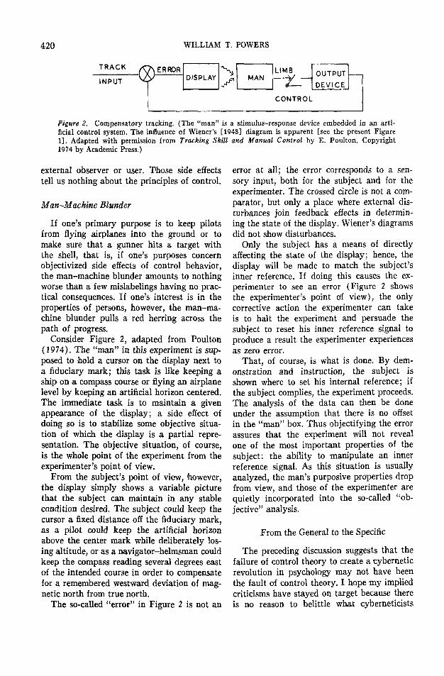
Figure 2. Compensatory tracking. (The "man" is a stimulus-response device embedded in an arti-ficial control system. The influence of Wiener's [1948] diagram is apparent [see the present Figure1], Adapted with permission from Tracking Skill and Manual Control by E. Poulton. Copyright1974 by Academic Press.)
A ERRORDISPLAY "S
y MANLIMy OUTPUT
</— - 1 DEVICE
CONTROL
external observer or user. Those side effectstell us nothing about the principles of control.
Man-Machine Blunder
If one's primary purpose is to keep pilotsfrom flying airplanes into the ground or tomake sure that a gunner hits a target withthe shell, that is, if one's purposes concernobjectivized side effects of control behavior,the man-machine blunder amounts to nothingworse than a few mislabelings having no prac-tical consequences. If one's interest is in theproperties of persons, however, the man-ma-chine blunder pulls a red herring across thepath of progress.
Consider Figure 2, adapted from Poulton(1974). The "man" in this experiment is sup-posed to hold a cursor on the display next toa fiduciary mark; this task is like keeping aship on a compass course or flying an airplanelevel by keeping an artificial horizon centered.The immediate task is to maintain a givenappearance of the display; a side effect ofdoing so is to stabilize some objective situa-tion of which the display is a partial repre-sentation. The objective situation, of course,is the whole point of the experiment from theexperimenter's point of view.
From the subject's point of view, however,the display simply shows a variable picturethat the subject can maintain in any stablecondition desired. The subject could keep thecursor a fixed distance off the fiduciary mark,as a pilot could keep the artificial horizonabove the center mark while deliberately los-ing altitude, or as a navigator-helmsman couldkeep the compass reading several degrees eastof the intended course in order to compensatefor a remembered westward deviation of mag-netic north from true north.
The so-called "error" in Figure 2 is not an
error at all; the error corresponds to a sen-sory input, both for the subject and for theexperimenter. The crossed circle is not a com-parator, but only a place where external dis-turbances join feedback effects in determin-ing the state of the display. Wiener's diagramsdid not show disturbances.
Only the subject has a means of directlyaffecting the state of the display; hence, thedisplay will be made to match the subject'sinner reference. If doing this causes the ex-perimenter to see an error (Figure 2 showsthe experimenter's point o'f view), the onlycorrective action the experimenter can takeis to halt the experiment and persuade thesubject to reset his inner reference signal toproduce a result the experimenter experiencesas zero error.
That, of course, is what is done. By dem-onstration and instruction, the subject isshown where to set his internal reference; ifthe subject complies, the experiment proceeds.The analysis of the data can then be doneunder the assumption that there is no offsetin the "man" -box. Thus objectifying the errorassures that the experiment will not revealone of the most important properties of thesubject: the ability to manipulate an innerreference signal. As this situation is usuallyanalyzed, the man's purposive properties dropfrom view, and those of the experimenter arequietly incorporated into the so-called "ob-jective" analysis.
From the General to the Specific
The preceding discussion suggests that thefailure of control theory to create a cyberneticrevolution in psychology may not have beenthe fault of control theory. I hope my impliedcriticisms have stayed on target because thereis no reason to belittle what cyberneticists

ANALYSIS OF PURPOSIVE SYSTEMS 421
have done or what engineering psychologistshave discovered. The blunders I have de-scribed are principally blunders of omissionand misinterpretation that have unnecessarilybut unavoidably limited the scope of theseendeavors. I shall commit blunders of my ownjust like these, as will we all. That is thepenalty for trying something new.
In trying to develop control theory as atool for experimental psychology, I think it isimportant to avoid assuming that any exampleof behavior involves a control organization. Ihave been critical of some psychologists foradopting a language that periodically assertsa model by calling every action a "response,"but I succumb to the same kind of temptationmyself when trying to convey my own pointof view. A basic analysis cannot be very con-vincing if its conclusions are plugged in wherethe premises are supposed to go, so in thefollowing section, the treatment will begin inas general a form as possible.
Let us assume little more than the earlybehaviorists did, and in some respects, let usassume a great deal less. The organism willbe treated as nothing more than a connectionbetween one set of physical quantities in theenvironment (input quantities) and anotherset of physical quantities in the environment(output quantities). By leaving the form ofthe organism function general, however, wewill allow for possibilities that were tacitlyruled out at the turn of the century, the mostimportant one being the possibility of a secu-larly adjustable constant term in the systemfunction. That term will ultimately turn intothe observable evidence of an inner purpose,although I will not pursue that point vigor-ously here.
This approach will explicitly recognize thefact that the inputs to an organism are af-fected not only by extraneous events but pos-sibly by the organism's own actions. By leav-ing the development general, we will be ableto deal deductively with feedback effects, notasserting them but simply stating the observa-ble conditions under which they necessarilyappear and those under which they can be ig-nored. Thus, the classical mechanistic cause-effect model will become a subset of the pres-ent analysis.
Let us now turn to mathematical tools,beginning with an approach that is neither asdetailed as possible nor as general as possiblebut that is, to my taste, just right (naturally).
The Quasi-static Approach
A quasi-static approach is one in whichphysical variables, although known to be sub-ject to dynamic constraints, are treated asalgebraic variables. In the physical sciences,this is a commonplace procedure. For example,the motions of the free ends of a lever aretreated as if the motions of one end were liter-ally simultaneous with the motions of theother end; inertia and transverse waves propa-gating along the lever are ignored. If a reallever is moved too rapidly, it will bounce offits fulcrum; one does not expect a quasi-staticanalysis to hold for such extreme cases.
The validity of the quasi-static approachas well as its usefulness depend on the fre-quency domain of interest. The designer of aman-machine system focuses on the high-fre-quency limits of performance because his taskis not to understand the man but to get themost out of the machine for some extraneouspurpose. This is the origin of the transferfunction approach, and the reason why theengineering models can get away with treat-ing the man in the system as an input-outputbox.
I am interested in the frequency domainthat lies between a pure steady state and the"corner frequency," where the quasi-staticanalysis begins to break down. Thus, the anal-ysis here does not encroach on the territoryof engineering psychology. In the present anal-ysis, there would be no point in carrying thetransient terms of interest in engineering psy-chology because they go to zero before theybecome important. There would be a positivedisadvantage in using mathematical formsthat map the space being investigated into anintuitively unrecognizable space with non-physical variables in it ("cisoidal oscillations"or imaginary quantities found in Laplacetransform theory and commonly applied tocontrol systems; see Starkey, 1955, p. 31).The following analysis, while of little use formeasuring transfer functions in the normal

422 WILLIAM T. POWERS
way, is suited to the elucidation of the struc-ture of behavioral organization.
A Quasi-static Analysis
Consider a behaving system ("system" forshort) in relationship to an environment. Thesystem is the simplest possible: It has onesensory input affected by an input quantity,q\, and one output that affects an outputquantity, q0. Both (ft and q0 are ordinaryphysical quantities in the environment or elseare regular functions of measurable physicalquantities.
In general, a change at the input to thesystem will result in a change at the outputbecause of intervening system characteristics.The output quantity will be related to manyother external quantities, but the only one ofinterest here is qi, the input quantity. Theinput quantity will also be subject to dis-turbances from variables that change or re-main constant independently of the output ofthe system.
The assumption of dynamic stability ismade: After any transient disturbance, thesystem-environment relationship will come toa steady-state equilibrium quickly enough topermit ignoring transient terms in the differ-ential equations that actually describe the re-lationship. This assumption implies the useof an averaging time or a minimum time reso-lution appropriate to each individual system.
It should not be thought that this assump-tion limits us to a static case. In the equationF = MA, or force equals mass times accelera-tion, the algebraic variable A is really thesecond derivative of position with respect totime. Nevertheless, there are many useful andaccurate applications of this algebraic formulain dynamic situations. In a great variety ofsituations, time-dependent variables can bedealt with quasi-statistically simply by aproper definition of the variables. All that islost is the ability to predict behavior near thedynamic limits of performance in terms ofthe chosen variables. The system equation is
9o = j(q\), f being a generalalgebraic function. (1)
(Small letters will be used for functions and
capital letters for multipliers of parenthesizedexpressions when ambiguity is possible.)
The environment equation contains twoterms representing linearly superposed contri-butions from two sources, which together de-termine completely the state of the inputquantity. One contribution comes from theoutput of the system via qa. The magnitudeof qa contributes an amount £(#0), where gis a general algebraic function describing thephysical connection from q0 to q\: This is thefeedback path, which is missing when #(90)is identically zero.
All other possible influences on the inputquantity that are independent of qa aresummed up as an equivalent disturbing quan-tity, q&, contributing to the state of qt throughan appropriately defined physical link sym-bolized as the function h; the magnitude ofthe contribution from disturbing quantities isthus h(q&). This provides the following en-vironment equation (see Figure 3):
?i = g(<Io) + h(q&)- (2)
The assumption of dynamic stability per-mits treating the system and environmentequations as a simultaneous pair. To find ageneral simultaneous solution valid for allquasi-static cases in which physical continuityexists, we shall rearrange Equations 1 and 2into equally general forms that are more ma-nipulable. First, a Taylor series expansion of/(<?i) is performed around a special (and asyet undefined) value, q^*, and an expansionof £(#0) is done about the corresponding spe-cial value £0*. For /((ft), the factor (<?i — <7i*)is factored out of the variable terms, leavingthe following quotient polynomial:
A, B,C, and so on are the Taylor coefficients.The quotient polynomial is symbolized as Uto yield the following working system equa-tion:
+U(ql-ql*). (3)
In a parallel manner, with the quotientpolynomial symbolized as V, g ( q 0 ) is repre-sented as g(q0*) + V(q0 - q0*) to yield the

ANALYSIS OF PURPOSIVE SYSTEMS 423
DISTURBANCEFUNCTION
h
DISTURBINGQUANTITY
SYSTEMINPUT FUNCTION
QUANTITY
T gFEEDBACKFUNCTION
OUTPUT
0 QUANTITY
Figure 3. Relationships among variables and functions in the quasi-static analysis. (The topo-logical similarity of Wiener's [1948] diagram, adapted in the present Figure 1, is of no significancebecause these variables and functions all pertain to observables outside the organism. This is nota model of the organism; it is a model of the organism's relationships to the external world.)
working environment equation of
Let the special value of qit or qi*, be de-fined as the value of q^ when there is no netdisturbance: h(q&) = 0. Then q\* = g(q0*)and g0* =/(<?!*). Substitutions into Equa-tions 3 and 4 then yield
(5)- q f )
and
qi-qi*=V(qa-q0*)+k(qi). (6)
Substitution of Equation 6 into Equation 5produces, after some manipulations twice in-volving the equivalence V(q0 — q0*) = g(q0)— g(qa*), Equation 7:
- UV,
where UV ̂ 1. (7)
Substituting from Equation 5 into Equation6 directly yields Equation 8:
where UV ̂ 1. (8)
The dimensions of U are change of outputper unit change of input, and the dimensionsof V are change of input per unit change o'foutput. Thus, the product UV is a dimension-less (and variable) number. It is customarilycalled the loop gain in morphologically simi-lar equations of control theory.
So far these equations remain completelygeneral, applying to any system-environmentrelationship of the basic form assumed, when
the assumption of dynamic stability is ob-served to hold true. No model of the internalorganization of the behaving system has beenassumed, nor has it been assumed that we aredealing with a control system or even a feed-back system. The only limits set on non-linearity of the functions are practical ones:Systems that are radically nonlinear are notlikely to meet the assumption of dynamic sta-bility. These prove to be quite permissivelimits.
Classifying System-EnvironmentRelationships
The behavior of a system as denned herecan be classified according to the observedmagnitude and sign of the loop gain, UV. Aseverely nonlinear system can conceivablypass from one class to another during behavior.
Type Z: Zero Loop Gain
If the product UV is zero because the func-tion / is zero, there is no behaving system.If it is zero because the function g is zero,there is no feedback and the simultaneoussolution of the equations becomes (fromEquations 1 and 2)
?o = /(?!)= /[*(?<)].
This is the open-loop case and correspondsto the classical cause-effect model of behavior.If (ft is considered a proximal stimulus (lo-cated at the sensory interface or even at somestage of perceptual processing inside the sys-tem) and 9a a distal stimulus, then the output

424 WILLIAM T. POWERS
or behavior is mediated by the organism ac-cording to the form of the function /, andthe proximal stimulus is the immediate causeof behavior. A stimulus object or event op-erates from its distal position as qA, affectingthe proximal stimulus (ft through interveningphysical laws described by the function h.Thus, a simple lineal causal chain links thedistal stimulus to the behavior.1
I shall say Z system to mean a behavingsystem in this Type Z relationship to its en-vironment. In order to show that a givenorganism should be modeled as a Z system, itis necessary to establish that the organism'sown behavior has no effect on the proximalstimuli in the supposed causal chain. I be-lieve that this condition is, in any normalcircumstance, impossible to meet. I will showlater that even separating stimulus and re-sponse in time will not make the Z-systemmodel acceptable.
Type P: Positive Loop Gain
If UV is positive and not zero, there is aType P, or positive feedback, relationship be-tween system and environment. The behavingsystem is then acting as a P system. Thistype of relationship is dynamically stable onlyfor UV < 1. A dynamic analysis is needed toshow what happens for UV ;> 1; the algebraicequations give spurious answers. The P sys-tem goes unconditionally into self-sustainedoscillations that either continue at a constantamplitude or increase exponentially or simplyhead for positive or negative infinite valuesof its variables. Whichever 'happens, the quasi-static analysis breaks down, as does the be-havior of the system, since this is not gen-erally considered normal behavior. A Type Prelationship is dynamically stable only for0<UV<1.
There have been qualitative assertions inthe literature that positive feedback may bebeneficial because it "enhances" or "amplifies"responses. Such assertions are uninformed.Positive feedback does amplify the responseto a disturbance because in a Type P rela-tionship, behavior aids the effects of the dis-turbance on the input quantity. Equation 7can be used to calculate the amplifying effectsof various amounts of positive feedback, with
the amplification factor being UV/(l — UV).The following list is an example of these cal-culations:
UV
.5
.6
.7
.8
.9
.99
Amplificationfactor
1.01.52.34.09.0
99.0unstable
In a nonlinear system, UV varies with themagnitude of disturbance; furthermore, natu-ral systems have muscles that fatigue andinteract with environments having variableproperties. These facts are incompatible withthe narrow range of values df UV (shownabove), in which any useful amount of am-plification is obtained from positive feedback.The relationship would always be on thebrink of instability under the best of circum-stances. We may expect natural P systems tobe rare.
Type N: Negative Loop Gain
If UV is negative and not zero there is aType N, or negative feedback, relationshipbetween system and environment. The sys-tem is an N system. UV may have any nega-tive value. In N systems, preservation of dy-namic stability requires a trade-off betweenthe magnitude of UV and the speed of re-sponse of the system. Servo-engineers wouldrecognize the great advantage we have hereover the person who has to design such asystem: The designer has to tailor the dy-namic characteristics to make the system-en-vironment relationship stable; we only haveto observe that it actually is stable. The equa-tions we are using would be of no help to adesigner of control systems.
It is difficult to find an example of behav-ior in which the 'feedback connection g is
1 Lineal means occurring along a line or in simplesequence, as in lineal feet. Linear means described bya firstrdegree equation: For example, the equationy = 3* expresses a linear relationship between x andy, while y = 3* +!/* expresses a nonlinear relation-ship.
ANALYSIS OF PURPOSIVE SYSTEMS 425
missing; feedback is clearly present in mostcircumstances. Moreover, it is generally foundthat organisms are sensitive to small changesof stimuli and that feedback effects are pro-nounced, so the magnitude of UV must beassumed in general to be large. Since we donot commonly observe dynamic instability, itfollows that the sign of U must be oppositeto that of V, that is, that the feedback isnegative and the system an N system jundermost circumstances. Detailed investigation ofindividual cases, of course, will settle thequestion. I hope, however, that it can be seenthat the Type N relationship is an importantone. We shall examine its properties.
Properties of the Type N relationship. Onthe right side of Equation 7 is the expressionUV/'(\ — UV), a form familiar in everymathematical approach to closed-loop anal-ysis. With UV being dimensionless and nega-tive for N systems, this expression is a dimen-sionless negative number between 0 and —1.Furthermore, the larger the minimum valueof —UV becomes, the more nearly UV/(l —UV) approaches the limiting value — 1. Whenthis limiting value is closely approached, wecan call the system an ideal N system.
In the experiments to be described, the typi-cal minimum value of UV estimated from thedata was —30. Thus, only a 3% error is en-tailed in saying that subjects behaved as idealN systems, in which ( — UV) is extremelylarge.
For an ideal N system, Equations 7 and 8reduce to especially simple forms:
and
(7a)
(8a)
From these equations can be drawn twobasic statements that characterize a widevariety of N systems but more accurately forthose that approach the ideal N system.Equation 7a is easier to translate if we re-member that #!* = g(q0*). The term g(q0)represents the effect of the output on the in-put quantity, h(qA) represents the effect ofthe disturbance on the input quantity, andq0* is the value of the output when there isno disturbance acting. It follows that the
change in the output quantity away from theno-disturbance case is just what is requiredto produce effects on the input quantity thatcancel the effects of the disturbance. Equation8a expresses the consequence of this cancella-tion: The input quantity remains at its un-disturbed value, <?i*. Thus, the actions of anN system, mediated by the feedback path,stabilize its input quantity against the effectsthat disturbances otherwise would have. Anideal N system does this perfectly.
It will be seen that the widespread notionthat negative feedback systems control theiroutputs is a misconception. In an artificialcontrol system designed to produce outputsof interest to a user, the feedback function gis selected to make sure that gt is preciselyrelated to some objective consequence of q0,so that controlling gi will indeed result in con-trolling the objective consequence of qa] 'how-ever, such systems are built to protect them-selves from all disturbances that might affect<7i directly. The erroneous transfer of an en-gineering model directly into a behavioralmodel was the cause of the misconception.The engineering model would show a refer-ence input to the system, the effect of whichwould be to adjust the setting of q\* and alsoto indirectly affect the objective consequence.As mentioned, no such input from the out-side exists in natural N systems (in none ofthose, at any rate, that I have investigated).
A behavioral illusion. Solving Equation 7afor qa produces
Compare this form with the equation for aZ system:
The difference in sign is a matter of choiceof coordinates, and the constant gi* can beused as the zero of the measurement scale, sothe forms are essentially the same. The pri-mary difference is that the organism function/ in the Z-system equation is replaced by theinverse of the feedback function g-1 in theN-system equation.
This comparison reveals a behavioral il-lusion of such significance that one hesitatesto believe it could exist. If one varies a distal
426 WILLIAM T. POWERS
stimulus <7d and observes that a measure ofbehavior q0 shows a strong regular dependenceon <7d, there is certainly a temptation to as-sume that the form of the dependence revealssomething about the organism. Yet, the com-parison we have just seen indicates that theform of the dependence may reflect only prop-erties of the local environment. The night-mare of any experimenter is to realize toolate that his results were forced by his ex-perimental design and do not actually per-tain to behavior. This nightmare has a goodchance of becoming a reality for a numberof behavioral scientists. An example may bein order.
Consider a bird with eyes that are fixed inits head. If some interesting object, say, abug, is moved across the line o'f sight, thebird's head will most likely turn to follow it.The Z-system or open-loop explanation wouldrun about like this: The bug's position, thedistal stimulus, is translated by optical ef-fects into a proximal stimulus on the retina,exciting sensory nerves and causing the ner-vous system to operate the muscles that turnthe head. This causal chain is so preciselycalibrated and its form so linear that themovement of the head exactly compensatesfor the movement of the bug. The image thusstays centered on the retina.
There is a reason why this kind of explana-tion skips so rapidly across the proximalstimulus. If the head tracks the bug perfectly,the image of the bug will remain stationaryon the retina, as indeed it very nearly does.But if the image remains stationary or wan-ders unsystematically about one point, thecausal chain cannot be followed through. Theopen-loop explanation contradicts itself.
If the angle o'f the head is q0 and the visualangle of the bug is qA, q<> has precisely asmuch effect as q& has on qi} the position ofthe retinal image. By choosing units properly,therefore, we can say that both g and h areunity multipliers of opposite sign. The twofunctions reflect the laws of geometric opticsand, hence, are exquisitely precise and linear.
Equation 7a predicts that for an ideal Nsystem, the output will vary as the inverseg function of the effect of the disturbance.Thus, the relationship between q& and qa will
be as precise and linear as the laws of geo-metric optics. The organism function /, on theother hand, may be both nonlinear and vari-able over time. As long as the polynomial Uremains large enough, the apparent behaviorallaw will be unaffected.
Thus, in the relationship between bug move-ment and head turning, we are not seeing thefunction / that describes the bird; instead,we anp seeing the function g that describes thephysics of the feedback effects. This propertyof N systems is well known to control engi-neers and to those who work with analog com-puters. It is time behavioral scientists becameaware of it, whatever the consequences.
Operant Conditioning
The quasi-static analysis works quite wellin at least one kind of operant-conditioningexperiment: the fixed-ratio experiment, inwhich an animal provides 'food for itself on aschedule that delivers one pellet of food foreach n presses of a lever.
The function g becomes just l/n, and thereis no disturbance [h(qA) = 0].a The environ-ment equation reduces to
qi = q«/n. (9)The average rate of reinforcement is treatedas being the input quantity. The equationsfor an ideal control system predict thatqi = gi*, which is to say that the organismwill keep the average rate of reinforcementat a level qi* that is determined by a propertyof the organism. The average rate of bar press-ing, using Equation 7a, will be qtt = nq{*.
From Equation 7a, we can predict what willhappen if the schedule is changed from »ito «2. The corresponding rates of bar pressing,qol and go2, will be related by
q0i/Qo2 = «i/»2. (10)The more presses are required to deliver onepellet, the more rapidly, in direct proportion,will the animal work the lever. This is a well-known empirical observation, found while"shaping" behavior to very high response rates.
A disturbance could be introduced by add-ing food pellets to the dish where pellets are
2 Excessive efforts, on extreme schedules, would in-troduce a disturbance.

ANALYSIS OF PURPOSIVE SYSTEMS 427
delivered by the lever pressing at a rate q&(the function h is then 1). The environmentequation would then be
<7i = Qo/n + <7a- (11)
From the solution for an ideal N system, wefind
?o = »(tfi* — ?d)- (12)
If (ft* is the observed rate of reinforcementin the absence of the disturbance, the rate oflever pressing in the presence of arbitrarilyadded food can be predicted. The averagepressing rate will drop as the rate of addingfood rises. When food is added arbitrarily ata rate just equal to qf, lever pressing will justcease. This prediction is in accord with scien-tific observation (Teitelbaum, 1966) and withthe qualitative empirical generalization thatnoncontingent reinforcement redu'ces behavior.8
It is evident that in order to predict quan-titatively the results of this kind of operant-conditioning experiment, all one needs to as-sume about the organism is that it is anideal N system. The value of gt* can be foundwith one observation, and a whole family ofrelationships can be predicted thereafter.Conversely, the information obtained aboutthe organism in such an experiment is onlythat it does act as an ideal N system con-trolling the rate of reinforcement. This anal-ysis, while not dealing with learning, showsthat changes of behavior do not necessarilyimply any change of behavioral organization.
Let us now turn to a second quantitativemethod, which will be discussed more brieflybut needs to be discussed because it dealswith time delays, which the quasi-static ap-proach cannot handle.
A Time-State Analysis withDynamic Constraints
One persistent and incorrect approach tofeedback phenomena is to treat an organismas a Z system, with any feedback effects beingtreated as if they occurred separately, afterone response and before the next, thus ap-parently permitting the system itself to bedealt with in open-loop fashion. Qualitatively,this seems to work; but, as in every open-loop analysis, the approach fails quantita-tively. The knowledge-of-results or stimulus-
response-stimulus-response . . . analysis seemsto succeed only because of the limitations ofverbal or qualitative reasoning.
I shall use a linear model here, so I canfocus on the main point without excessivecomplication. Let us alternate between the or-ganism and the environment, first calculatingthe magnitude of the output quantity that re-sults from the current magnitude of input andthen calculating the next value of the inputfrom the value of the output and the magni-tude of the (constant ) disturbance. This pro-cedure leads to two modified equations. Thesystem equation will be
qi*)t> (13)
(14)
and the environment equation will be
HqA.
The functions /, g, and h have been trans-lated into linear multipliers F, G, and H; anda time index, t, has been introduced. The loopgain is now the product FG, which corre-sponds to UV previously.
To skip a useless analysis, I will report thatthis set of equations converges to a steadystate with FG in the range between +1 and— 1 but not at or outside those limits. Withthe loop gain FG limited to FG > -1, thebehaving system certainly cannot act like anideal N system. The permissible amount offeedback is so small that there would belittle behavioral effect from having any at all(except possible proneness to instability).
The difficulty here is that a sequential-stateanalysis of this kind introduces time withouttaking into account phenomena that dependon time. In the design of logic circuits, thiscan perhaps be done successfully, although atight design has to recognize the fact thatso-called "binary variables" in a logic networkare really continuous physical quantities that,like any quantities in the macroscopic world,take time to change from one state to another.Ones and zeros exist only in abstract machines.
Without getting into a full dynamic anal-ysis, we can introduce a dynamic constrainton this system by allowing the output to
8 This is an excellent experimental method for mea-suring QI* in a natural situation.

428 WILLIAM T. POWERS
change only a fraction of the way from itscurrent value of q0(t) toward the next com-puted value of F(qi — q f ) (t) during the timebetween one value of t and the next. LettingK, a number between 0 and 1, be this frac-tion, let us introduce a modified system equa-tion with this dynamic constraint:
<7o<*+i) = Qo(t) +. (15)
Substituting Equation 14 into Equation 15now yields
FHq& -
KFG- K)
or
qi*). (16)
A steady state for repeated calculationswith Equation 16 will be reached in one jumpif (1 + KFG — K) =0, implying an opti-mum value for K of
Kopt=l/(l-FG). (17)
Setting g0(*+2) = ?o<o leads to the valueof K at which the system just goes into end-less oscillation, that is, the critical value orupper limit of K:
KCIii = 2/(l-FG)=2Kovt. (18)
If Kovt < K < K.<,rit, the successive itera-tions -of Equation 16 oscillate above and be-low the steady-state solution, converging moreand more rapidly as K approaches Koft. For0 < K < Kopt, the successive iterations ap-proach the same steady state but in an ex-ponential monotonic way. In any case, thesteady state (ss) is that found by substituting#opt into Equation 16, with the result
- FG\~G~ ~ ~For /?G« —1 (an ideal N system), the ex-
pression FG/(1 — FG) can be replaced by— 1 to yield
Gg0(8B) = ?i* - Hq*. (20)
Comparing this with Equation 7a,
one can see that the linear sequential-stateanalysis with a dynamic constraint providesthe same final picture of behavior that thequasi-static analysis provides. Treating be-havior as a succession of instantaneous eventspropagating around a closed loop will notyield a correct analysis, no matter how tinythe steps are made, unless this dynamic con-straint is properly introduced. With the dy-namic constraint, the discrete analysis showsthat behavior follows the same laws of nega-tive feedback whether the feedback effectsare instantaneous or delayed. This considera-tion has not, to my knowledge, been takeninto account in other discrete analyses ofbehavior.
I have found this iterative approach usefulin constructing computer simulations; evenfor highly nonlinear systems, it is usuallypossible to find a value of K that will stabilizethe model. The behavior is essentially thatof a system with a first-order lag.
Experimental Demonstrations of Principle
Let us now look at six experiments thatbring out fundamental aspects of this ap-proach. They are not thought experiments,although I will describe them only in generalterms; they were done with an on-line com-puter system using real subjects. The aim ofthe experiments was not to begin serious ex-plorations of human nature using these or-ganizing principles; that task lies in the future(and I hope I will not be the only one in-volved in it). The purpose of this effort hasbeen to select from among dozens of experi-ments tried over the past 3 years a few thatare easily replicated by many means thatproduce reliable results that can be explainedonly by the version of control theory usedhere and that always give accurate quantita-tive results, as good as those obtained in thelaboratory demonstrations in introductoryphysics courses. Of course, the point of theseexperiments will be lost if nobody else triesthem.
There is a way to tell when one has thor-oughly understood each experiment and hasdiscarded all inappropriate points of view.This is to persist until it is seen exactly whyeach quantitative result occurs as it does.

ANALYSIS OF PURPOSIVE SYSTEMS 429
When one realizes that no other outcome ispossible for an ideal N system, one fully un-derstands the experiment and also how anideal N system works. To communicate thatkind of understanding is what I hope for here.
General Experimental Method
A practiced subject sits facing a cathode-ray tube(CRT) display while holding the handle of a con-trol stick that is pivoted near the subject's elbow.The angle of the control stick above the horizontalis considered the positive direction of behavior, be-low being the negative, and a digitized version ofthat measure in the computer is defined as the outputquantity qa.
On the screen is a short horizontal bar of lightthat can move up and down only over a grid ofdots that remains stationary, providing a referencebackground. The position of the bar, or cursor, aboveor below center is taken as the input quantity, itsmeasure being the digital number in the computercorresponding to displayed position qi. This remotelydefined 91 is valid because there are no disturbancesintervening between subject and display that couldalter the perceived figure-ground pattern.
Inside the computer is a random-number routinethat repeats only after 37,000 hours of running time.Another routine smooths this random number, limit-ing its band width to about .2 Hz. The resultingnumber is the disturbing quantity q&. The subjecthas no way to sense the magnitude of qt directly.
The position of the cursor is completely deter-mined at every instant (that is, 60 times per sec)by the sum of qa and ?j. When all quantities areexpressed in terms of equivalent units on the screen,the environment equation corresponding to Equa-tion 1 is
9i = 9o + gd. (21)
The system equation is just Equation 1: qa= f ( q i ) ,where / is some general quasi-static algebraic func-tion. The handle position is thus taken to dependin some way on the sensed position of the cursor,
A typical run begins with g« forced to zero. Dur-ing this time, the value of 91 is determined. By defi-nition, this value is gi*. It is always measured, eventhough the instructions may appear to predetermineit; subjects do not always set qi in the way the ex-perimenter had in mind. A typical run lasts 60 secafter the random-number program is allowed to con-tinue. The random-number generator runs continu-ously, but for the first part of each experiment,zero is substituted for the output of the smoothingroutine. So far no two experimental runs have em-ployed the same pattern of disturbances. If this seemslike excessive zeal to attain randomness, it is donebecause a critic once suggested, apparently seriously,that the sine-wave disturbances I used at first werebeing memorized by the subject, even though therewas no way for the subject to detect errors in phase
DOWN
BOUNDARYTIM£-»
Figure 4. Experiment 1 results drawn from thecathode-ray tube (CRT) display of data. (The"cursor" trace represents the up-down positionfluctuations that the subject sees on the CRT screen.The "disturbance" trace represents the invisible ran-dom quantity that is added to a representation ofhandle position ["handle" trace] to determine theposition of the cursor.)
or amplitude between the subject's actions and thechanges in the disturbance and no way to sense thedisturbance.
Experiment 1: Basic Relationships
The subject is requested to hold the cursoreven with the center row of background dots(a standard compensatory tracking experi-ment). The value of #1* is determined asabove, and the run commences. From Equa-tions 7a and 8a, which presume that the sub-ject is an ideal N system, it is predicted thatqi = £i* and q0 = qi* — gd. Here, qi* shouldbe zero and very nearly is.
Figure 4 is a drawing of a typical resultfrom a plot on the CRT screen. Any practicedsubject will produce this kind of pattern.
The root mean square (RMS) variationsof qi about qf (= 0 here) are about plus orminus 2% o'f full scale. Thus, q0 is, within thesame tolerance, a mirror image of the dis-turbance q&.
A minimum value of U can be estimatedfrom a simulation that best fits the data. Formost practiced subjects, it is at least —30and may be much larger. The data suggest afirst-order lag system (output proportional tointegral of qi — qi*), but no attempt wasmade to determine a valid transfer function.The assumption of stability is clearly met.There is little doubt that we are seeing anearly ideal N system.
The best way to gain an intuitive under-standing of Figure 4 is to start with the ob-

430 WILLIAM T. POWERS
UP
DOWN
DISTURBANCE
BEGINS
TIME
DOWN
Figure 5. Experiment 3 results drawn from the cathode-ray tube (CRT) display of the data. (Theupper trace shows the behavior of the cursor [<?i] on the CRT screen without [left] and with[right] the disturbance acting. The lower trace shows the handle position [g0] with no disturbanceacting [left] and the handle position [?«] and disturbance magnitude [?a] when disturbancebegins changing [right]. The output, not the input, directly reflects the disturbance. The durationof the run was about 1 minute.)
served fact that the input quantity remainsessentially at the value qi*. It follows thatthe handle must always be in the positionthat balances out the effect of the disturb-ance. We are not modeling the interior of thesubject, so we need not worry about how thiseffect is created. It is a fact to be accepted.From the fact that the input is stabilized, theother relationships follow.
Experiment 2: Unspecified qi*
The subject is now asked to hold the cur-sor in "some other position," as accurately aspossible. With q& — 0, qi* is measured, andthe run commences. The results are the sameas before, with a nonzero value of qi*. Thisvariation on Experiment 1 shows that the sub-ject, not the apparatus or die experimenter,determines a specific quantitative setting of<?.*.
Experiment 3: Change of Variable
The subject is asked to make the cursormove in any slow rhythmic pattern, the samepattern throughout the run. The subject in-
dicates when the pattern on the screen (withq& — 0) is the one to be maintained. The runcommences. The initial pattern is taken to be<7i*; there are many means for characterizinga temporal pattern quasi-statistically, such asphase, amplitude, or frequency measures (oneor more of which might prove to be controlledor uncontrolled). I used a much more sub-jective method, adequate for present purposesalthough not for serious work: eyeballing thedata.
A typical result is shown in Figure 5. Aseparate plot is given for q\ to avoid con-fusing the curves. Without any disturbance,the measure of handle behavior is the sameas the measure of the input quantity. Regu-larities in the cursor behavior appear to bejust reflections of regularities in the handlebehavior. When the disturbance is applied tothe cursor, however, it is the handle behav-ior, not the cursor behavior, that begins toshow corresponding large random fluctuations.This is not at all what the customary cause-effect model would predict.
Two major points are illustrated here. One
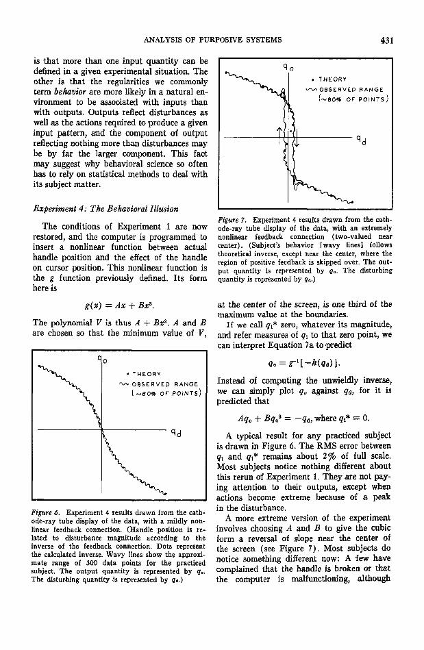
ANALYSIS OF PURPOSIVE SYSTEMS 431
is that more than one input quantity can bedenned in a given experimental situation. Theother is that the regularities we commonlyterm behavior are more likely in a natural en-vironment to be associated with inputs thanwith outputs. Outputs reflect disturbances aswell as the actions required to produce a giveninput pattern, and the component of outputreflecting nothing more than disturbances maybe by far the larger component. This factmay suggest why behavioral science so oftenhas to rely on statistical methods to deal withits subject matter.
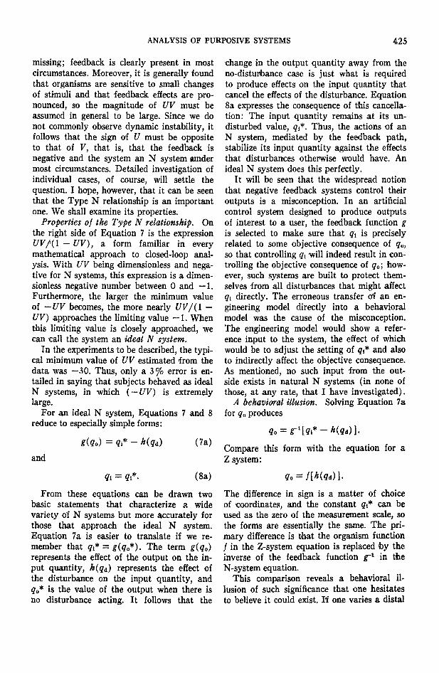
Experiment 4: The Behavioral Illusion
The conditions of Experiment 1 are nowrestored, and the computer is programmed toinsert a nonlinear function between actualhandle position and the effect of the handleon cursor position. This nonlinear function isthe g function previously denned. Its formhere is
g(x) = Ax + Bx».
The polynomial V is thus A + Bx2. A and Bare chosen so that the minimum value of V,
T H E O R Y
O B S E R V E D RANGE80% or POINTS)
Figure 6. Experiment 4 results drawn from the cath-ode-ray tube display of the data, with a mildly non-linear feedback connection. (Handle position is re-lated to disturbance magnitude according to theinverse of the feedback connection. Dots representthe calculated inverse. Wavy lines show the approxi-mate range of 300 data points for the practicedsubject. The output quantity is represented by 0o.The disturbing quantity is represented by ?a.)
. T H E O R Y
N^OBSERVED RANGE
(~ao» OF POINTS)
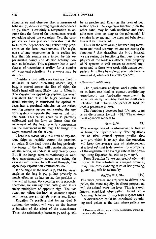
Figure 7. Experiment 4 results drawn from the cath-ode-ray tube display of the data, with an extremelynonlinear feedback connection (two-valued nearcenter). (Subject's behavior [wavy lines] followstheoretical inverse, except near the center, where theregion of positive feedback is skipped over. The out-put quantity is represented by q». The disturbingquantity is represented by ?a.)
at the center of the screen, is one third of themaximum value at the boundaries.
If we call <?i* zero, whatever its magnitude,and refer measures of q{ to that zero point, wecan interpret Equation 7a to predict
Instead of computing the unwieldly inverse,we can simply plot qa against q&, for it ispredicted that
AqQ + Bq0* = -q&, where ?i* = 0.
A typical result for any practiced subjectis drawn in Figure 6. The RMS error betweenqi and eft* remains about 2% of full scale.Most subjects notice nothing different aboutthis rerun of Experiment 1. They are not pay-ing attention to their outputs, except whenactions become extreme because of a peakin the disturbance.
A more extreme version of the experimentinvolves choosing A and B to give the cubicform a reversal of slope near the center ofthe screen (see Figure 7). Most subjects donotice something different now: A few havecomplained that the handle is broken or thatthe computer is malfunctioning, although
432 WILLIAM T. POWERS
V ° OUTPUT
HANDLED
DISTURBANCES
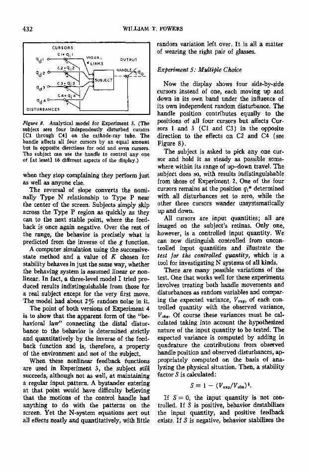
Figure 8. Analytical model for Experiment 5. (Thesubject sees four independently disturbed cursors[Cl through C4] on the cathode-ray tube. Thehandle affects all four cursors by an equal amountbut in opposite directions for odd and even cursors.The subject can use the handle to control any oneof [at least] 16 different aspects of the display.)
when they stop complaining they perform justas well as anyone else.
The reversal of slope converts the nomi-nally Type N relationship to Type P nearthe center of the screen. Subjects simply skipacross the Type P region as quickly as theycan to the next stable point, where the feed-back is once again negative. Over the rest ofthe range, the behavior is precisely what ispredicted from the inverse of the g function.
A computer simulation using the successive-state method and a value of K chosen 'forstability behaves in just the same way, whetherthe behaving system is assumed linear or non-linear. In fact, a three-level model I tried pro-duced results indistinguishable from those fora real subject except for the very first move.The model had about 2% random noise in it.
The point of both versions of Experiment 4is to show that the apparent form of the "be-havioral law" connecting the distal distur-bance to the behavior is determined strictlyand quantitatively by the inverse of the feed-back function and is, therefore, a propertyof the environment and not of the subject.
When 'these nonlinear feedback functionsare used in Experiment 3, the subject stillsucceeds, although not as well, at maintaininga regular input pattern. A bystander enteringat that point would have difficulty believingthat the motions of the control handle hadanything to do with the patterns on thescreen. Yet the N-system equations sort outall effects neatly and quantitatively, with little
random variation left over. It is all a matterof wearing the right pair of glasses.
Experiment 5: Multiple Choice
Now the display shows four side-by-sidecursors instead of one, each moving up anddown in its own band under the influence ofits own independent random disturbance. Thehandle position contributes equally to thepositions of all four cursors but affects Cur-sors 1 and 3 (Cl and C3) in the oppositedirection to the effects on C2 and C4 (seeFigure 8).
The subject is asked to pick any one cur-sor and hold it as steady as possible some-where within its range of up-down travel. Thesubject does so, with results indistinguishablefrom those of Experiment 2. One of the fourcursors remains at the position qf determinedwith all disturbances set to zero, while theother three cursors wander unsystematicallyup and down.
All cursors are input quantities; all areimaged on the subject's retinas. Only one,however, is a controlled input quantity. Wecan now distinguish controlled from uncon-trolled input quantities and illustrate thetest for the controlled quantity, which is atool for investigating N systems of all kinds.
There are many possible variations of thetest. One that works well for these experimentsinvolves treating both handle movements anddisturbances as random variables and compar-ing the expected variance, Fexp, of each con-trolled quantity with the observed variance,Fobs- Of course these variances must be cal-culated taking into account the hypothesizednature of the input quantity to be tested. Theexpected variance is computed by adding inquadrature the contributions from observedhandle position and observed disturbances, ap-propriately computed on the basis of ana-lyzing the physical situation. Then, a stabilityfactor 5 is calculated:
If S = 0, the input quantity is not con-trolled. If S is positive, behavior destabilizesthe input quantity, and positive feedbackexists. If S is negative, behavior stabilizes the

ANALYSIS OF PURPOSIVE SYSTEMS 433
input quantity, and negative feedback exists.For 5 several standard deviations more nega-tive than —1, the behaving system can becalled an ideal control system. For experi-ments like the first three, S is typically —4to —9 for the controlled cursor, implying thatthe chances against an N system existingrange from one in thousands to one in billions.For uncontrolled cursors, S ranges from +1to —1 on short runs and comes close to 0 onlong (10-minute) runs.
This statistical version of the test shouldbe useful in cases where behavior takes placein a natural environment, where there aremany possible effects of behavior, manysources of disturbance, and many potentiallycontrolled quantities affected both by behav-ior and by disturbances. Once a controlledquantity has been found by this statisticalapproach, use can be made of the more quan-titative methods of analysis previously dis-cussed.
Any version of the test for the controlledquantity must be followed by verifying thatan apparent controlled quantity must besensed by the behaving system in order to becontrolled. In the present experiments, cover-ing up the appropriate cursor with a card-board strip should, and does, cause the con-trolled quantity to become an uncontrolledone. Covering any or all of the other cursorshas no effect at all.
Experiment 6: More-AbstractControlled Quantities
Under the same conditions as Experiment5, the subject is asked to hold constant someother aspect of the display (not specified bythe experimenter) rather than the position ofone of the cursors. Most subjects are initiallybaffled by this request, some permanently un-til given broad hints. Eventually, most see thepossibilities o'f the fact that the handle af-fects odd and even cursors oppositely. Oneaspect is the difference in position between anodd and an even cursor. A subject can easilykeep, say, Cl and C4 level with each otheror Cl a fixed distance above or below C4.Both cursors wander up and down but alwaystogether. With suitable definitions, a con-trolled quantity can be found that unequivo-
cally passes the test for the controlled quan-tity (four possibilities of this type exist).
Another type of controlled quantity is theconfiguration with three cursors lying along astraight line. Four possible controlled quan-tities of this type exist. Still another involvescreating a fixed angle with one cursor centeredat the vertex and the other two lying in thesides of the angle. All these are relatively easyto control once the subject has realized thatthey can be seen in the display. Only 1 ofthese 16 possible static controlled quantitiescan be controlled at a time 'because the con-trol handle has only one degree of freedom.
What determines which controlled quantitywill be controlled? The apparatus obviouslydoes not, for it determines only the possibil-ities; not the behavior either—the output,with its single degree of 'freedom, affects allpossible controlled quantities all of the time.The behaving system itself must be the deter-mining factor. What the person attends tobecomes the controlled aspect of the display.The person also determines the particularstate of the selected aspect that is to serveas (ft*. My efforts to make models of humanorganization have been aimed at explainingthis type of phenomenon. It has been diffi-cult at times to explain why such models arerequired when the listener is unaware thatsuch phenomena exist.
In all these experiments, a typical correla-tion coefficient relating handle position to anoncontrolled quantity or its associated dis-turbance is in the range from 0 to .8. Statis-tics are poor in these short runs, but somecorrelations do occur even in long runs. Thehandle and the disturbances do affect thevarious cursors; correlations are to be ex-pected there.
The correlation between a controlled quan-tity and either its associated disturbance orthe handle position is normally lower than .1;a well-practiced subject will frequently pro-duce a correlation of zero to two significantfigures. At the same time, the correlation be-tween magnitude of disturbance and handleposition is normally higher than .99 (I canoften reach .998 in the simpler experiments).To appreciate the meaning of these figures,one has to remember that the subject cannot

434 WILLIAM T. POWERS
sense any of the disturbances except throughtheir effects on the input quantities, the cur-sor positions.
If the controlled input quantity shows acorrelation of essentially zero with the be-havior, any standard experimental designwould reject it as contributing nothing to thevariance of behavior. But the disturbance thatcontributes essentially 100% of the varianceof the behavior can act on the organism onlyvia the variable that shows no significant cor-relation with behavior. Not only the oldcause-effect model breaks down when one isdealing with an N system, the very basis ofexperimental psychology breaks down also.
Summary and Conclusions
I have examined in this article four mis-takes that threw cybernetics off the track asfar as psychology is concerned: (a) thinkingof control theory as a machine analogy, (b)focusing on objective consequences of behav-ior of no importance to the behaving systemitself, (c) misidentifying reference signals assensory inputs, and (d) overlooking purpo-sive properties of human behavior in man-machine experiments. Considering behavior,without going through any technological anal-ogy, I have developed two mathematical toolsfor analyzing and classifying behaving orga-nisms. The classical cause-effect model isincluded as a special case. Finally, I haveintroduced six experiments that illustrateclasses of phenomena peculiar to control be-havior and that cannot be explained underany paradigm but the control system model.(The last statement can be taken as a friendlychallenge.)
I believe that the concepts and methods ex-plored here are the basis for a scientific revo-lution in psychology and biology, the revolu-tion promised by cybernetics 30 years agobut delayed by difficulties in breaking free ofolder points of view. Kuhn (1970) uses theterm paradigm in the sense I mean when Isay that control theory is a new paradigmfor understanding life processes—not only in-dividual behavior but the behavior of bio-chemical and social systems. Chapter X inKuhn's book discusses "Revolutions as
Changes in World View." The experimentswe have seen here, while not of great im-portance in themselves, represent my attemptto show how control theory allows us to seethe same facts of behavior that have alwaysbeen seen but through new eyes, new organiz-ing principles, and new views of the world ofbehavior.
The natural tendency of any human beingis to deal with the unfamiliar by first tryingto see it as the nearest familiar thing. That iswhat happened to the basic concepts of cy-bernetics. It will happen even more pro-nouncedly in response to the ideas we havelooked at here. The difficulties faced by anew paradigm, as Kuhn explained so clearly,result not from battles over how to explainparticular conceptual puzzles, but from by-passing altogether old puzzles that some peo-ple insist for a long time still need solving.There are still many fruitful areas of researchand many unsolved problems concerning theproperties of phlogiston. Modern observationaland data-processing techniques in astronomycould lead to great (but unwanted) improve-ments in the predictive accuracy of the epi-cycle model of planetary motions (I knew agraduate student in astronomy who showedhow well epicycles could work with the aidof a large computer).
Control theory bypasses the entire set ofempirical problems in psychology concerninghow people tend to behave under various ex-ternal circumstances. One kind of behaviorcan appear under many different circum-stances; instead of comparing all the variouskinds of causes with each other while lookingfor objective similarities to explain the com-mon effects, we are led by control theory tolook for the inputs that are disturbed not onlyby the discovered causes but by all possiblecauses. For a thousand unconnected empiricalgeneralizations based on superficial similar-ities among stimuli, I here substitute one gen-eral underlying principle: control of input.
References
Chapanis, A. Men, machines, and models. AmericanPsychologist, 1961, 16, 113-131.
Kelley, C. R. Manual and automatic control. NewYork: Wiley, 1968.

ANALYSIS OF PURPOSIVE SYSTEMS 435
Kuhn, T. The structure of scientific revolutions.Chicago: University of Chicago Press, 1970.
Maslow, A. H. The farther reaches of human nature.New York: Viking, 1971.
Mayr, O. The origins of feedback control. Cam-bridge, Mass.: MIT Press, 1970.
McDougall, W. The hormic psychology. In A. Adler(Ed.), Psychologies of 1930. Worcester, Mass.:Clark University Press, 1931.
Poulton, E. Tracking skill and manual control. NewYork: Academic Press, 1974.
Powers, W. T. Behavior: The control of perception.Chicago: Aldine, 1973.
Powers, W., Clark, R., & McFarland, R. A generalfeedback theory of human behavior. Part 1. Per-ceptual and Motor Skills Monograph, 1960, 11(1,Serial No. 7). (a)
Powers, W., Clark, R., & McFarland, R. A generalfeedback theory of human behavior. Part 2. Per-ceptual and Motor Skills Monograph, 1960, 77(3,Serial No. 7). (b)
Rosenblueth, A., Wiener, N., & Bigelow, J. Behavior,purpose, and teleology. In W. Buckley (Ed.),
Modern systems research for the behavioral scien-tist. Chicago: Aldine, 1968.
Skinner, B. F. The behavior of organisms. NewYork: Appleton-Century-Crofts, 1938.
Skinner, B. F. Freedom and the control of man. InB. F. Skinner (Ed.), Cumulative record. NewYork: Appleton-Century-Crofts, 1972.
Starkey, B. J. Laplace transformations for electricalengineers. New York: Philosophical Library, 1955.
Teitelbaum, P. The use of operant methods in theassessment and control of motivational states. InW. K. Honig (Ed.), Operant behavior. New York:Appleton-Century-Crofts, 1966.
Tolman, E. C. Purposive behavior in animals andman. New York: Century, 1932.
Von Foerster, H., White, J., Peterson, L., & Russell,J. (Eds.). Purposive systems. London: Macmillan,1968.
Wiener, N. Cybernetics: Control and communicationin the animal and the machine. New York: Wiley,1948.
Received April 14, 1978 •