Quantitative Evaluation of a Novel Image Segmentation Algorithm

Francisco J. Estrada and Allan D. JepsonDepartment of Computer Science

University of TorontoToronto, ON., M5S 3G4, Canada{strider,jepson}@cs.utoronto.ca

Abstract

We present a quantitative evaluation of SE-MinCut, anovel segmentation algorithm based on spectral embeddingand minimum cut. We use human segmentations from theBerkeley Segmentation Database as ground truth and pro-pose suitable measures to evaluate segmentation quality.With these measures we generate precision/recall curvesfor SE-MinCut and three of the leading segmentation algo-rithms: Mean-Shift, Normalized Cuts, and the Local Varia-tion algorithm. These curves characterize the performanceof each algorithm over a range of input parameters. Wecompare the precision/recall curves for the four algorithmsand show segmented images that support the conclusionsobtained from the quantitative evaluation.

1 Introduction

Image segmentation continues to be a challenging prob-lem. Despite continuous improvements, the task of accu-rately segmenting an arbitrary image remains basically un-solved. At the same time, only recently has a significant ef-fort been dedicated to developing suitable quantitative mea-sures of segmentation quality that can be used to evaluateand compare segmentation algorithms.

In this paper we present a quantitative evaluation of anovel technique that uses spectral embedding together withthe minimum-cut algorithm to generate high quality seg-mentations. We compare SE-MinCut against three of theleading image segmentation algorithms: the Mean-Shift al-gorithm of Comaniciu and Meer [5, 6], the NormalizedCuts algorithm of Shi and Malik [16], and the Local Vari-ation algorithm of Felzenszwalb and Huttenlocher [10].The algorithms are evaluated on the Berkeley SegmentationDatabase [14, 13], which provides human segmentations fora large collection of images.

The contributions of our paper are: 1) A simple def-inition of precision and recall measures for segmentation

quality, these measures are sensitive to over- and under-segmentation and can be computed efficiently. 2) The intro-duction of precision/recall curves that characterize the seg-mentation quality of a given algorithm. These curves allowfor a robust comparison of segmentation quality that is in-dependent of the choice of input parameters. 3) A quantita-tive evaluation and comparison of segmentation quality forthe four segmentation algorithms over the complete BSDwhich, to our knowledge, is the first direct comparison ofcurrent segmentation algorithms presented in the literature.

We will start with an overview of the SE-MinCut frame-work and place it in the context of current research involv-ing minimum-cut for image segmentation. We will thenshow segmentation results for the four algorithms on im-ages from the BSD, proceed to the complete quantitativeevaluation of the algorithms, and discuss our results.

2 Spectral Embedding and Min-Cut

The minimum cut algorithm is a graph-partitioning tech-nique that has received a significant amount of attention inrecent years as a useful framework for image segmentation.Any image I(~x) can be viewed as a graph G(V,E) whereV is a set of nodes that correspond to pixels in the image,and E is a set of edges that connect nodes in the graph. E isusually set up so that only neighboring pixels are connected,and the strength of the connection between two pixels isgiven by the weight of the edge that spans them. The graphG(V,E) is usually stored as an affinity matrix. For an n×mimage, we can build an nm × nm affinity matrix A whoseelements Ai,j are proportional to the similarity between pix-els i and j and correspond to the weight of the edges Ei,j .Given this affinity matrix, the min-cut algorithm computesthe subset of edges Ei,j that must be removed from G(V,E)so that the graph is partitioned into two disjoint sets, and thesum of weights for the removed edges is minimal.

Computation of the minimum cut usually involves defin-ing two special nodes called source and sink that are linkedto elements within one of the disjoint sets in G(V,E).

The cut itself can be computed using a max-flow formula-tion [4]. The minimum cut framework is attractive for sev-eral reasons: the min-cut separating source and sink nodescan be computed efficiently [2, 4], it is guaranteed to be aglobal minimum, and given appropriate source and sink re-gions, the resulting cut will partition an image along salientimage boundaries. Several algorithms have been proposedthat use minimum cut for image segmentation, Wu andLeahy [18] propose trying every pair of pixels as source andsink and selecting from the resulting partitions the cut withthe minimum weight, while Veksler [17] proposes placingsink regions outside the image and using individual imagepixels as source. However, both of these techniques can be-come impractical due to the large number of partitions thathave to be computed. At the same time, the final selectedcut may not correspond to salient image structure. Boykovet al. [2, 1] on the other hand, rely on user interaction to se-lect suitable source and sink regions to produce a segmenta-tion efficiently. Finally, Boykov et al. [3] propose a methodto optimize an initial label field using min-cut to performlabel swap and region expansion operations.

2.1 Spectral Embedding

We will briefly review the algorithm proposed in [8],which uses spectral embedding to define suitable sourceand sink regions for min-cut. The algorithm uses a simpleaffinity measure based on the grayscale difference betweenneighboring pixels

Ai,j = e−(I(~xi)−I(~xj))2/(2σ2), (1)

where σ represents the typical gray-level variation betweenneighboring pixels. Without loss of generality, we assumeA is sparse, and the entries Ai,j are non-zero only for ele-ments within the 5×5 pixel neighborhood centered at pixel~xi (although any neighborhood structure including the com-plete image can be used).

We generate a Markov matrix M by normalizing thecolumns of A using Dj ≡

∑nmk=1 Ak,j , and Mi,j =

Ai,j/Dj . M defines a Markov chain representing a ran-dom walk over image pixels (see Meila and Shi [15]). Letpt(~xj) denote the probability that a particle undergoing therandom walk is at pixel ~xj at time t, and let the nm di-mensional vector ~pt represent pt(~x). We can estimate ~pt+1

using~pt+1 = M~pt, where M = AD−1, (2)

and D is a diagonal matrix formed by the normalizationfactors Dj .

Given an initial distribution ~p0, it follows from (2)that the distribution after t steps of the random walk is~pt = M t~p0. Here, M t can be expressed in terms of itseigenvectors and eigenvalues, obtained conveniently from

12

3

4

5

6

7

8

910

1112

13

1415

16 17

1819

20

21

22

23

24 2526

27

28

29

30

31

32

−20 −10 0 10 20−25

−20

−15

−10

−5

0

5

10

15

20

25

z2 x 1000

z 3 x 1

000

1

2 3

4

5

6

7 8

910

11

12

13

14

15

16

1718

19

20

21

22

23

24

25

26

27

28

29

3031

32

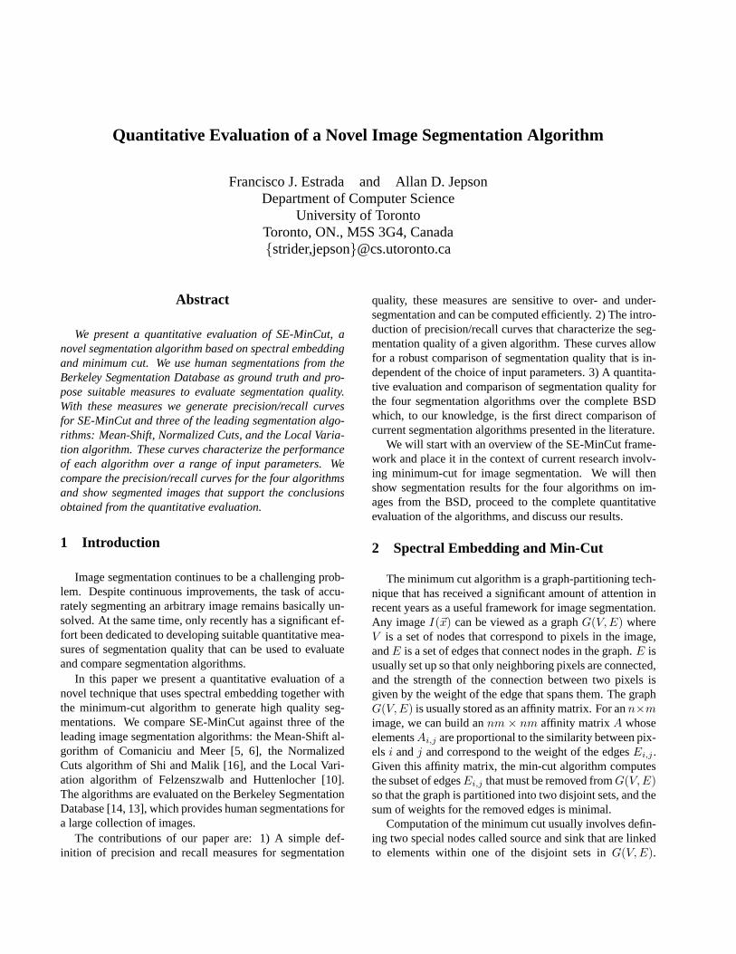
Figure 1. Fractal image (3 regions plus noise,100 × 100 pixels), seed regions generated byour algorithm, second and third componentsof the embedding, and final segmentation.For this image d = 15 and t was calculatedso that |λd+1|

t ' 1/3.

the similar, symmetric matrix L = D−1/2MD1/2 =D−1/2AD−1/2. Since L is symmetric, its eigendecompo-sition has the form L = U∆U T , where U is an orthogonalmatrix whose columns are the eigenvectors of L, and ∆ isa diagonal matrix of eigenvalues λi, i = 1, . . . , nm. Weassume that the eigenvalues have been sorted in decreasingorder of magnitude. It can be shown from the shape of Dand A that λi ∈ (−1, 1] and that at least one eigenvalue isequal to 1. So, without loss of generality, we assume thatλ1 = 1. This eigenvalue problem is equivalent to that of Shiand Malik [16] except for the choice of the affinity matrix.

From the eigendecomposition of L and (2) we obtain

~pt = M t~p0 = (D1/2U)∆t(U T D−1/2)~p0. (3)

Suppose that we start the random walk at pixel ~xi. Theinitial distribution is given by ~p0,i = ~ei, which is a vectorwith 1 in the ith row and zeros elsewhere. Then, after tsteps of the random walk, we obtain the diffused distribu-tion ~pt,i = M t~ei, which we call a blur kernel. Since theprobability that a particle will jump across a strong imageboundary is small, blur kernels will diffuse little across suchboundaries, and the stronger the boundary, the smaller thediffusion across it. As a result of this, blur kernels for pixelsseparated by a strong boundary will have their probabilitymasses distributed over different subsets of pixels, and theirinner product ~p T

t,i~pt,j must vanish. Conversely, blur kernelsfor neighboring pixels in homogeneous regions will be sim-

ilar, and their inner product will be large.We approximate these blur kernels using only the top d

eigenvectors and eigenvalues of the Markov matrix M

~pt,i ' ~qt,i ≡ (D1/2Ud)~wt,i, (4)

where ~wt,i = ∆tdU

Td D−1/2~ei is the projected blur ker-

nel for pixel ~xi at time t, Ud contains the first d columnsof U , and ∆d is a d × d diagonal matrix formed with thefirst d eigenvalues λi. We can approximate the inner prod-uct of the original blur kernels with ~p T

t,i~pt,j ' ~q Tt,i~qt,j =

~wTt,iQ~wt,j , with Q = U T

d DUd. Defining ~zt,i = Q1/2 ~wt,i

we have ~q Tt,i~qt,j = ~z T

t,i~zt,j . The approximation error de-pends on the magnitude of the terms |λi|

t for i > d, thelargest of which is |λd+1|

t. We find a good approximationwhen d and t are chosen so that |λd+1|

t < 1/3. Fig. 1bshows a plot of two of the dimensions in the embedding.Other properties and details of the embedding are discussedin [8].

2.2 Seed Region Selection

The projected blur kernels cluster in the d-dimensionalspace induced by the embedding. Because blur kernels fromhomogeneous image regions are similar to one another,these clusters correspond to local groups of similar pixels.Furthermore, the density of blur kernels between neighbor-ing clusters is indicative of whether there is a smooth con-tinuation between the groups of pixels corresponding to theclusters. A low density valley between two clusters indi-cates the existence of an image boundary.

To find clusters, we map the ~z points onto the unit sphere~st,i = ~zt,i/||~zt,i||, and generate a set of initial guesses forthe cluster centers {~mk}

Kk=1 by randomly sampling points

from ~st,i. Successive samples are constrained to have aninner product of at least τ0 from previous samples withτ0 = 0.8. The number of clusters K is chosen to be themaximum number of samples that can be drawn before allpoints ~st,i have an inner product of at least τ0 with somecenter ~mk, this ensures that we have enough clusters to spanthe embedding.

The location of each cluster center ~mk is then updatediteratively by computing a weighted average of the points~st,i in the neighborhood of ~mk

~m′k =

∑~s T

t,i~mk≥τ1

(~sTt,i ~mk)~st,i

∑~s T

t,i~mk≥τ1

(~sTt,i ~mk)

. (5)

The weights correspond to the inner product between thepoints ~st,i and the current estimate for the cluster center.Only the points on the unit sphere whose inner product withregard to the cluster center is greater than a threshold τ1

contribute to the weighted average. In what follows we useτ1 = 0.95.

The resulting cluster centers can be used to define seedregions in the image that consist of groups of similar pix-els. Seed region Sk originating from cluster k is obtainedby thresholding the inner products of ~st,i with ~mk, Sk ≡{~xj |~s

Tt,j ~mk ≥ τ1}. Seed regions obtained in this fashion

are illustrated in Fig. 1. Notice here two important prop-erties of the seed regions: they include a significant frac-tion of the image area, and they do not cross salient imageboundaries. Combinations of seed regions are used to de-fine source and sink nodes for min-cut. Details about howthis is accomplished are found in [8].

We compute a minimum cut for every source/sink com-bination and store the resulting partitions. After all thecuts are done, we generate an intermediate segmentation asthe intersection of all the partitions generated by min-cut.This intermediate segmentation is usually over-segmented,so we perform an additional stage of region merging. Re-gion merging is performed by examining the distributionof links along the boundary between two regions. For parti-tions that correspond to salient image boundaries most linksshould be weak (smaller than .1 in our case). If less than acertain portion τm of the links along the boundary are suit-ably weak, we merge the regions.

2.3 Experimental Results

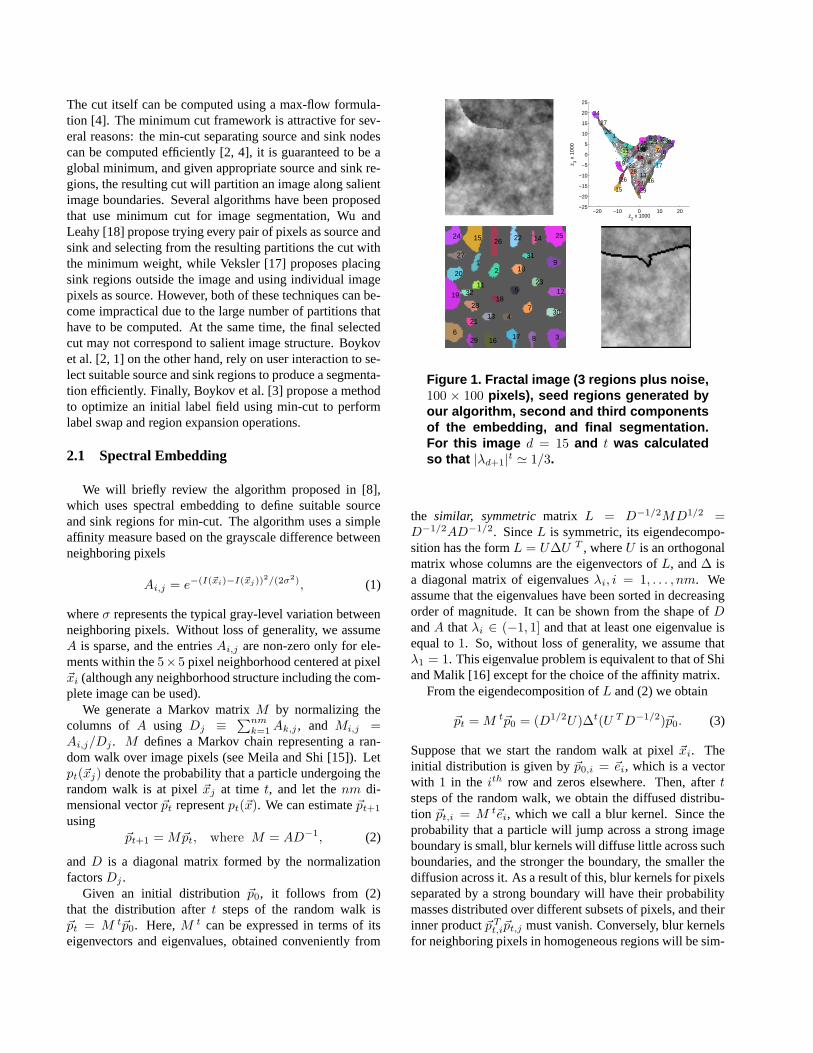
Figure 2 shows the segmentation results generated withour algorithm on several images from the Berkeley Segmen-tation Database (BSD) [13]. Results generated with Nor-malized Cuts [16], Mean Shift [5, 6], and the Local Varia-tion [10] algorithm are shown for comparison. The choiceof parameters for each algorithm is noted in the figure andis based on the comparative graphs described in the nextsection. These results indicate that the regions extractedwith our algorithm better capture the perceived structure ofthe images, and the boundaries of regions are more closelyaligned with salient image boundaries (this is an expectedresult of the use of min-cut). The next section presentsa quantitative comparison of the segmentation results pro-duced with the four algorithms on the BSD.

3 Comparing Segmentation Algorithms

The images in Fig. 2 offer compelling evidence that oursegmentation algorithm performs well on a variety of im-ages from different domains. Such visual comparisons havebeen used extensively in the past as a means of illustratingthe capabilities of segmentation algorithms. However, wewould like a quantitative measure of segmentation qualitythat can be used to compare the algorithms directly.

In this section, we will evaluate the performance ofour algorithm on the Berkeley Segmentation Database(BSD) [13]. We will discuss the organization of the BSD,

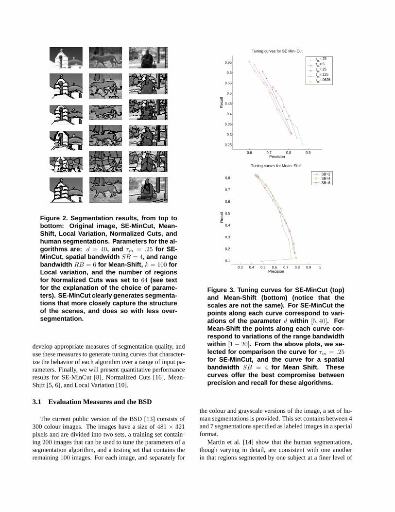
Figure 2. Segmentation results, from top tobottom: Original image, SE-MinCut, Mean-Shift, Local Variation, Normalized Cuts, andhuman segmentations. Parameters for the al-gorithms are: d = 40, and τm = .25 for SE-MinCut, spatial bandwidth SB = 4, and rangebandwidth RB = 6 for Mean-Shift, k = 100 forLocal variation, and the number of regionsfor Normalized Cuts was set to 64 (see textfor the explanation of the choice of parame-ters). SE-MinCut clearly generates segmenta-tions that more closely capture the structureof the scenes, and does so with less over-segmentation.

develop appropriate measures of segmentation quality, anduse these measures to generate tuning curves that character-ize the behavior of each algorithm over a range of input pa-rameters. Finally, we will present quantitative performanceresults for SE-MinCut [8], Normalized Cuts [16], Mean-Shift [5, 6], and Local Variation [10].

3.1 Evaluation Measures and the BSD

The current public version of the BSD [13] consists of300 colour images. The images have a size of 481 × 321pixels and are divided into two sets, a training set contain-ing 200 images that can be used to tune the parameters of asegmentation algorithm, and a testing set that contains theremaining 100 images. For each image, and separately for

0.3 0.4 0.5 0.6 0.7 0.8 0.9 1

0.1

0.2

0.3

0.4

0.5

0.6

0.7

0.8

Precision

Rec

all

Tuning curves for Mean−Shift

SB=2SB=4SB=8

0.6 0.7 0.8 0.9

0.25

0.3

0.35

0.4

0.45

0.5

0.55

0.6

0.65

Precision

Re

call

Tuning curves for SE Min−Cut

τm

=.75τm

=.5τm

=.25τm

=.125τm

=.0625

Figure 3. Tuning curves for SE-MinCut (top)and Mean-Shift (bottom) (notice that thescales are not the same). For SE-MinCut thepoints along each curve correspond to vari-ations of the parameter d within [5, 40]. ForMean-Shift the points along each curve cor-respond to variations of the range bandwidthwithin [1 − 20]. From the above plots, we se-lected for comparison the curve for τm = .25for SE-MinCut, and the curve for a spatialbandwidth SB = 4 for Mean Shift. Thesecurves offer the best compromise betweenprecision and recall for these algorithms.

the colour and grayscale versions of the image, a set of hu-man segmentations is provided. This set contains between 4and 7 segmentations specified as labeled images in a specialformat.

Martin et al. [14] show that the human segmentations,though varying in detail, are consistent with one anotherin that regions segmented by one subject at a finer level of

detail can be merged consistently to yield the regions ex-tracted by a different subject at a coarser level of detail.Based on this consistency, Martin et al. propose two mea-sures to evaluate segmentation performance and use them tocompare the Normalized Cuts algorithm against the humansegmentations. However, these measures are not sensitiveto over and under-segmentation (both of which can yieldlow error values). This effect was also noted by Martin [12]who proposed several alternative measures for comparingsegmentation algorithms. Among these, he discussed theuse of precision/recall values that characterize the agree-ment between the region boundaries of two segmentations.In his work, these measures are computed using a bi-partitematching formulation that matches boundary pixels usingtheir location and orientation.

Here we propose a simpler method for matching bound-aries between a source segmentation S1 and a target seg-mentation S2. Matching is performed by examining the im-mediate neighborhood of each boundary pixel bi in S1 forpotential matches. The neighborhood is searched in orderof increasing distance in a fixed pattern following the pixelgrid, up to a maximum distance of τd. Pixels are matched tothe nearest boundary element bx in S2 as long as there is noother boundary pixel bj in S1 between bi and bx. This pro-cedure allows for many-to-one matchings between bound-ary pixels, which is useful when corresponding boundariesin the two segmentations have different length due to smalllocalization errors. However, it is possible for (at most) twoboundaries in the source segmentation to be matched to thesame boundary in the target segmentation. This would oc-cur when the target boundary is ’sandwiched’ between thetwo boundaries from the source segmentation.

Using this matching strategy, we define precision and re-call to be proportional to the total number of unmatchedpixels between two segmentations S1 and S2. Unmatchedpixels are those for which a suitable match cannot befound within a particular distance threshold τd. Our pre-cision/recall measures are defined as follows:

Precision(S1, S2) =Matched(S1, S2)

|S1|, (6)

where Matched(S1, S2) is the number of boundary pixelsin S1 for which a suitable match was found in S2, and |S1|is the total number of boundary pixels in S1. Similarly

Recall(S2, S1) =Matched(S2, S1)

|S2|. (7)

Precision is low when there is significant over-segmentation, or when a large number of boundarypixels have localization errors greater than τd. A low recallvalue is typically the result of under-segmentation andindicates failure to capture salient image structure.

The principal advantage of using precision and recall forthe evaluation of segmentation results is that we can com-pare not only the segmentations produced by different al-gorithms, but also the results produced by the same algo-rithm using different input parameters. By systematicallychanging the value of the input parameters, we can producetuning curves that characterize the performance of a partic-ular segmentation technique for a wide range of its input pa-rameters, thus providing a more complete evaluation of thequality of the segmentations that can be generated with thatalgorithm. The tuning curves also allow for the selectionof input parameters that will yield the desired combinationof precision and recall within the operating range of eachalgorithm.

3.2 Experimental Setup

We will use the measures defined above to compare thesegmentations produced by the four algorithms. However,neither our algorithm nor the Normalized Cuts implemen-tation from [7] can work directly on the images from theBSD due to their size. In what follows, we will use thegrayscale images from the BSD after they have been appro-priately blurred and downsampled by a factor of 4 to a sizeof 121×88 pixels. The human segmentations of each imagehave also been downsampled to the appropriate size.

Since human segmentations of the same image vary inlevel of detail, precision and recall would change signifi-cantly depending on which target segmentation is chosen.Instead of comparing against individual human segmenta-tions, we choose to compare against a composite segmen-tation that is formed by the union of all region boundariesextracted by human observers for the same image. This hadalready been suggested by Martin [12]. Since the automaticsegmentation results and the human segmentations in theBSD consist of labeled images, we use an identical proce-dure to generate the region boundaries for all the segmen-tations involved. This procedure is simple and consists ofmarking as a boundary any pixel that has at least 1 neighborwith a different label.

We used the implementations of the algorithms madeavailable by the authors. For Normalized Cuts see [7], forLocal Variation see [9], and for Mean-Shift see [11]. Wetested each algorithm over a range of values for its input pa-rameters. Matching was carried out using a distance thresh-old τd = 5, which is reasonably large given the resolutionof the images. Since there is no training phase involved, weran each algorithm for each combination of input parame-ters over the full 300 images of the BSD. For each of theseruns, we calculate the median precision and recall valuesand use these values to generate tuning curves that charac-terize the algorithm’s performance. For algorithms with asingle input parameter (Normalized Cuts and Local Varia-

tion), we obtain a single curve. For algorithms with two pa-rameters (SE-MinCut, and Mean-Shift), we get a curve foreach value of one input parameter, while the values alongthe curve correspond to variations of the second parameter.The ranges for the input parameters of each algorithm weredetermined experimentally to produce significant over- andunder-segmentation at the extremes, while values withinthis range were chosen so as to yield segmentations withperceptible differences.

The input parameters and ranges are as follows: for Nor-malized Cuts, the only input parameter is the desired num-ber of regions; we tested the algorithm for values within[2, 128]. The Local Variation algorithm also takes a singleinput parameter k that roughly controls the size of the re-gions in the resulting segmentation (for details please referto [10]); smaller values of k yield smaller regions and favourover-segmentation. For this algorithm we tested values of kwithin [10, 1800].

For Mean-Shift we have two parameters: The spatialbandwidth and the range bandwidth. These parameters arerelated to the spatial and gray-level intensity resolution ofthe analysis (see [5, 6] for details). In practice, the segmen-tation software for Mean-Shift uses an additional parameter(the size in pixels of the smallest allowed region). We didn’ttest the effect of this parameter; since it only imposes an ar-tificial limit on over-segmentation, it was kept fixed at 25pixels (which is the same size as the search window usedfor boundary matching). Experimentation showed that thelargest differences between segmentations were obtainedwhen varying the range bandwidth parameter. Thus, weevaluated the algorithm using three values for the spatialbandwidth within [2, 8], and for each of these values, wecomputed a tuning curve that corresponds to variations ofthe range bandwidth within [1, 20].

For SE-MinCut, we tested two parameters. One is d,which determines the number of eigenvectors to use in theembedding. We then use d to determine t so that |λd+1|

t '1/3 as described in the previous section. The other pa-rameter is the merging threshold τm. The remaining in-ternal parameters mentioned in the text were kept fixed atthe original values proposed in [8]. The largest variationbetween segmentations is obtained by changing the valueof d. Following the same methodology used with Mean-Shift, we chose 5 values for the merging threshold between[1/16, 3/4], and for each of these we computed a tuningcurve that corresponds to variations of d within [5, 40].

Finally, we generated precision and recall data for hu-man segmentations. Given the set of human segmentationsfor a particular image, we selected each segmentation inturn and compared it against a composite of the remainingsegmentations for that same image. We then computed themedian precision and recall for all observers. The result-ing precision and recall points are useful for comparing the

0 0.2 0.4 0.6 0.8 10

0.1

0.2

0.3

0.4

0.5

0.6

0.7

0.8

0.9

1

Precision

Rec

all

Tuning Curves for all Algorithms

SE Min−CutMean ShiftLocal VariationNormalized CutsCannyHuman

Figure 4. Tuning curves for all segmenta-tion algorithms plus canny edges, and preci-sion/recall values for human segmentations.SE-MinCut clearly has the best performanceof all algorithms over its range of input pa-rameters.

performance of segmentation algorithms against human ob-servers.

4 Tuning Curves and Algorithm Comparison

Since we have 3 tuning curves for the Mean-Shift algo-rithm, and 5 curves for the SE-MinCut algorithm, we se-lected for comparison the curves that corresponds to the pa-rameter combinations that yield the best compromise be-tween precision and recall. Fig. 3 shows the tuning curvesobtained for SE-MinCut and Mean-Shift. We have chosenthe tuning curve that corresponds to τm = .25 as the rep-resentative for SE-MinCut, and the tuning curve that cor-responds to a spatial bandwidth SB = 4 is selected as therepresentative for Mean-Shift.

The selected curves for SE-MinCut and Mean-Shift to-gether with the curves for Normalized Cuts and Local Vari-ation are shown in Fig. 4. The figure also shows the pointsthat correspond to the median precision and recall of hu-man segmentations for the 300 images of the BSD. This fig-ure shows that SE-MinCut outperforms the other segmenta-tion algorithms across its range of input parameters. For agiven recall value, SE-MinCut achieves the highest preci-sion; conversely, for a given precision value, our algorithmachieves the best recall. This improved performance indi-

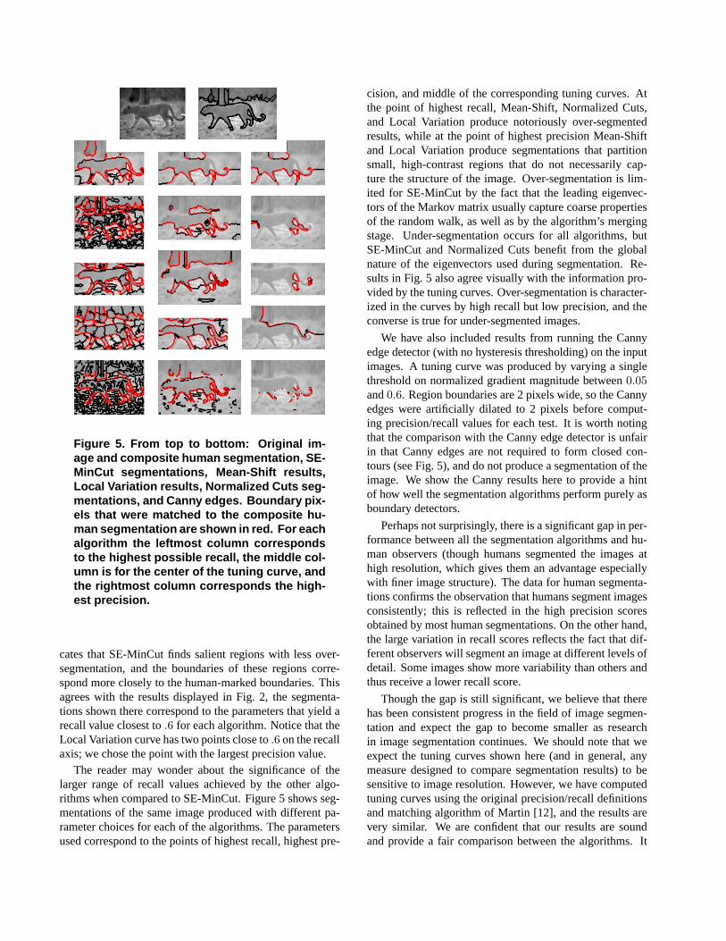
Figure 5. From top to bottom: Original im-age and composite human segmentation, SE-MinCut segmentations, Mean-Shift results,Local Variation results, Normalized Cuts seg-mentations, and Canny edges. Boundary pix-els that were matched to the composite hu-man segmentation are shown in red. For eachalgorithm the leftmost column correspondsto the highest possible recall, the middle col-umn is for the center of the tuning curve, andthe rightmost column corresponds the high-est precision.

cates that SE-MinCut finds salient regions with less over-segmentation, and the boundaries of these regions corre-spond more closely to the human-marked boundaries. Thisagrees with the results displayed in Fig. 2, the segmenta-tions shown there correspond to the parameters that yield arecall value closest to .6 for each algorithm. Notice that theLocal Variation curve has two points close to .6 on the recallaxis; we chose the point with the largest precision value.

The reader may wonder about the significance of thelarger range of recall values achieved by the other algo-rithms when compared to SE-MinCut. Figure 5 shows seg-mentations of the same image produced with different pa-rameter choices for each of the algorithms. The parametersused correspond to the points of highest recall, highest pre-

cision, and middle of the corresponding tuning curves. Atthe point of highest recall, Mean-Shift, Normalized Cuts,and Local Variation produce notoriously over-segmentedresults, while at the point of highest precision Mean-Shiftand Local Variation produce segmentations that partitionsmall, high-contrast regions that do not necessarily cap-ture the structure of the image. Over-segmentation is lim-ited for SE-MinCut by the fact that the leading eigenvec-tors of the Markov matrix usually capture coarse propertiesof the random walk, as well as by the algorithm’s mergingstage. Under-segmentation occurs for all algorithms, butSE-MinCut and Normalized Cuts benefit from the globalnature of the eigenvectors used during segmentation. Re-sults in Fig. 5 also agree visually with the information pro-vided by the tuning curves. Over-segmentation is character-ized in the curves by high recall but low precision, and theconverse is true for under-segmented images.

We have also included results from running the Cannyedge detector (with no hysteresis thresholding) on the inputimages. A tuning curve was produced by varying a singlethreshold on normalized gradient magnitude between 0.05and 0.6. Region boundaries are 2 pixels wide, so the Cannyedges were artificially dilated to 2 pixels before comput-ing precision/recall values for each test. It is worth notingthat the comparison with the Canny edge detector is unfairin that Canny edges are not required to form closed con-tours (see Fig. 5), and do not produce a segmentation of theimage. We show the Canny results here to provide a hintof how well the segmentation algorithms perform purely asboundary detectors.

Perhaps not surprisingly, there is a significant gap in per-formance between all the segmentation algorithms and hu-man observers (though humans segmented the images athigh resolution, which gives them an advantage especiallywith finer image structure). The data for human segmenta-tions confirms the observation that humans segment imagesconsistently; this is reflected in the high precision scoresobtained by most human segmentations. On the other hand,the large variation in recall scores reflects the fact that dif-ferent observers will segment an image at different levels ofdetail. Some images show more variability than others andthus receive a lower recall score.

Though the gap is still significant, we believe that therehas been consistent progress in the field of image segmen-tation and expect the gap to become smaller as researchin image segmentation continues. We should note that weexpect the tuning curves shown here (and in general, anymeasure designed to compare segmentation results) to besensitive to image resolution. However, we have computedtuning curves using the original precision/recall definitionsand matching algorithm of Martin [12], and the results arevery similar. We are confident that our results are soundand provide a fair comparison between the algorithms. It

is worth mentioning that SE-MinCut produces good qualitysegmentations using a simple gray-scale based affinity mea-sure. We expect that better affinity measures will enhancethe quality of the segmentations produced by our algorithm.

In terms of run-time, the best performance is achievedby the Local Variation algorithm, which takes around 1 sec.to segment images of the size used here; Mean-Shift takesbetween 1 and 7 sec. depending on the spatial bandwidthparameter; Normalized Cuts takes between 10 sec. and1.5 min. depending on the number of regions requested;finally, SE-MinCut takes between 1 and 7 min. depend-ing on the number of eigenvectors used for the embedding.These times were measured on a 1.9GHz Pentium IV ma-chine. Both Normalized Cuts and SE-MinCut are partly im-plemented in Matlab. In the case of SE-MinCut there arethree main components: the spectral embedding and regionproposal step, min-cut, and the merging stage. We expectthat the first and last of these components can be optimizedfor increased efficiency. Our goal here was to show thatmin-cut with automatic source and sink selection, followedby a simple post-processing stage can produce higher qual-ity segmentations than other current algorithms.

5 Conclusion

We have shown that the SE-MinCut algorithm is capa-ble of generating high quality segmentations using a simpleaffinity measure based on gray-scale similarity. We pre-sented simple precision and recall measures of segmenta-tion quality, and a matching algorithm that can be used tocompute them efficiently. With these measures, we eval-uated the quality of the segmentations produced by sev-eral well known algorithms over the Berkeley SegmentationDatabase, and presented tuning curves that characterize theperformance of these algorithms over a range of their inputparameters. This is to our knowledge the first quantitativecomparison of leading segmentation algorithms on a stan-dard set of images.

The tuning curves show that the SE-MinCut algorithmproduces better segmentations for any desired value of re-call within its tuning curve. Though the other algorithmshave a wider range of recall values, larger recall and pre-cision values come at the cost of significant over- or under-segmentation. It should be noted that there is no in-principlereason why finer structure cannot be segmented with SE-MinCut using the recursive approach that has also been pro-posed for Normalized Cuts. Specifically, once coarse re-gions have been extracted (and we know from the abovethat such regions are likely to agree closely with perceptu-ally salient image structure), each region can be individuallysegmented using SE-MinCut.

References

[1] Y. Boykov and M. Jolly. Interactive Graph Cuts for optimalboundary & region segmentation of objects in n-d images.In ICCV, pages 105–112, 2001.

[2] Y. Boykov and V. Kolmogorov. An experimental compar-ison of min-cut/max-flow algorithms for energy minimiza-tion in vision. In International Workshop on Energy Min-imization Methods in Computer Vision and Pattern Recog-nition, Lecture Notes in Computer Science, pages 359–374,2001.

[3] Y. Boykov, O. Veksler, and R. Zabih. Fast, approximateenergy minimization via graph cuts. PAMI, 23(11):1222–1239, 2001.

[4] Cherkassky and Goldberg. On implementing push-relabelmethod for the maximum flow problem. In Proc. IPCO-4,pages 157–171, 1995.

[5] D. Comaniciu and P. Meer. Robust analysis of featurespaces: Color image segmentation. In CVPR, pages 750–755, 1997.

[6] D. Comaniciu and P. Meer. Mean shift analysis and applica-tions. In ICCV, pages 1197–1203, 1999.

[7] T. Cour, S. Yu, and J. Shi. Normal-ized cuts matlab code. code available athttp://www.cis.upenn.edu/˜jshi/software/.

[8] F. J. Estrada, A. D. Jepson, and C. Chennubhotla. Spectralembedding and min cut for image segmentation. In BMVC,pages 317–326, 2004.

[9] P. Felzenszwalb and D. Huttenlocher. Image seg-mentation by local variation code. code available athttp://www.ai.mit.edu/people/pff/seg/seg.html.

[10] P. Felzenszwalb and D. Huttenlocher. Image segmentationusing local variation. In CVPR, pages 98–104, 1998.

[11] B. Georgescu and C. M. Christoudias. The Edge Detectionand Image SegmentatiON (EDISON) system. code availableat http://www.caip.rutgers.edu/riul/research/code.html.

[12] D. Martin. An Empirical Approach to Grouping and Seg-mentation. PhD thesis, University of California, Berkeley,2002.

[13] D. Martin and C. Fowlkes. The Berke-ley segmentation database and benchmark.http://www.cs.berkeley.edu/projects/vision/grouping/segbench/.

[14] D. Martin, C. Fowlkes, D. Tal, and J. Malik. A databaseof human segmented natural images and its application toevaluating segmentation algorithms and measuring ecologi-cal statistics. In ICCV, pages 416–425, 2001.

[15] M. Meila and J. Shi. Learning segmentation by randomwalks. In NIPS, pages 873–879, 2000.

[16] J. Shi and J. Malik. Normalized cuts and image segmenta-tion. PAMI, 2000.

[17] O. Veksler. Image segmentation by nested cuts. In CVPR,pages 339–344, 2000.

[18] Z. Wu and R. Leahy. An optimal graph theoretic approachto data clustering: Theory and its application to image seg-mentation. PAMI, 15(11):1101–1113, Nov. 1993.