R u t c o r

Research

R e p o r t

RUTCOR

Rutgers Center for

Operations Research

Rutgers University

640 Bartholomew Road

Piscataway, New Jersey

08854-8003

Telephone: 732-445-3804

Telefax: 732-445-5472

Email: rrr@rutcor.rutgers.edu

http://rutcor.rutgers.edu/∼rrr

Augmented Lagrangian and

Alternating Direction Methods

for Convex Optimization:

A Tutorial and Some

Illustrative ComputationalResults

Jonathan Ecksteina

RRR 32-2012, December 2012

aDepartment of Management Science and Information Systems (MSIS)and RUTCOR, Rutgers University, 640 Bartholomew Road, Piscataway, NJ08854-8003

Rutcor Research Report

RRR 32-2012, December 2012

Augmented Lagrangian and

Alternating Direction Methods

for Convex Optimization:

A Tutorial and Some

Illustrative ComputationalResults

Jonathan Eckstein

Abstract. The alternating direction of multipliers (ADMM) is a form of augmentedLagrangian algorithm that has experienced a renaissance in recent years due to itsapplicability to optimization problems arising from “big data” and image process-ing applications, and the relative ease with which it may be implemented in paralleland distributed computational environments. This chapter aims to provide an ac-cessible introduction to the analytical underpinnings of the method, which are oftenobscured in treatments that do not assume knowledge of convex and set-valued anal-ysis. In particular, it is tempting to view the method as an approximate version ofthe classical augmented Lagrangian algorithm, using one pass of block coordinateminimization to approximately minimize the augmented Lagrangian at each itera-tion. This chapter, assuming as little prior knowledge of convex analysis as possible,shows that the actual convergence mechanism of the algorithm is quite different, andthen underscores this observations with some new computational results in whichwe compare the ADMM to algorithms that do indeed work by approximately mini-mizing the augmented Lagrangian.

Acknowledgements: This material is based in part upon work supported by the NationalScience Foundation under Grant CCF-1115638. The author also thanks his student WangYao for his work on the computational experiments.Please insert the acknowledgement here.

Page 2 RRR 32-2012

1 Introduction

The alternating direction method of multipliers (ADMM) is a convex optimization algorithmdating back to the early 1980’s [10, 11]; it has attracted renewed attention recently due toits applicability to various machine learning and image processing problems. In particular,

• It appears to perform reasonably well on these relatively recent applications, betterthan when adapted to traditional operations research problems such as minimum-costnetwork flows.

• The ADMM can take advantage of the structure of these problems, which involveoptimizing sums of fairly simple but sometimes nonsmooth convex functions.

• Extremely high accuracy is not usually a requirement for these applications, reducingthe impact of the ADMM’s tendency toward slow “tail convergence”.

• Depending on the application, it is often is relatively easy to implement the ADMMin a distributed-memory, parallel manner. This property is important for “big data”problems in which the entire problem dataset may not fit readily into the memory ofa single processor.

The recent survey article [3] describes the ADMM from the perspective of machine learningapplications; another, older survey is contained in the doctoral thesis [5].

The current literature of the ADMM presents its convergence theory in two different ways:some references [17, 7, 8] make extensive use of abstract concepts from convex analysis andset-valued operators, and are thus somewhat inaccessible to many readers, while others [2, 3]present proofs which use only elementary principles but do not attempt to convey the “deepstructure” of the algorithm.

This paper has two goals: the first is to attempt to convey the “deep structure” of theADMM without assuming the reader has extensive familiarity with convex or set-valuedanalysis; to this end, some mathematical rigor will be sacrificed in the interest of clarifyingthe key concepts. The intention is to make most of the benefits of a deeper understandingof the method available to a wider audience. The second goal is to present some recentcomputational results which are interesting in their own right and serve to illustrate thepractical impact of the convergence theory of the ADMM. In particular, these results suggestthat it is not, despite superficial appearances, particularly insightful to think of the ADMMas an approximation to the classical augmented Lagrangian algorithm combined with a blockcoordinate minimization method for the subproblems.

The remainder of this paper is structured as follows: Section 2 describes the ADMMand a popular example application, the “lasso” or compressed sensing problem, and thenSection 3 summarizes some necessary background material. Section 4 presents the classicaugmented Lagrangian method for convex problems as an application of nonexpansive algo-rithmic mappings, and then Section 5 applies the same analytical techniqeus to the ADMM.Section 6 presents the computational results and Section 7 makes some concluding remarks

RRR 32-2012 Page 3

and presents some avenues for future research. The material in Sections 2-5 is not funda-mentally new, and can be inferred from the references mentioned in each section; the onlycontribution is in the manner of presentation. The new computational work underscores theideas found in the theory and raises some issues for future investigation.

2 Statement of the ADMM and a Sample Problem

Although it can be developed in a slightly more general form — see for example [3] — thefollowing problem formulation is sufficient for most applications of the ADMM:

minx∈Rn

f(x) + g(Mx). (1)

Here, M is an m×n matrix, often assumed to have full column rank, and f and g are convexfunctions on Rn and Rm, respectively. We let f and g take not only values in R but also thevalue +∞, so that constraints may be “embedded” in f and g, in the sense that if f(x) =∞or g(Mx) =∞, then the point x is considered to be infeasible for (1).

By appropriate use of infinite values for f or g, a very wide range of convex problems maybe modeled through (1). To make the discussion more concrete, however, we now describe asimple illustrative example that fits very readily into the form (1) without any use of infinitefunction values, and resembles in basic structure many of applications responsible for theresurgence of interest in the ADMM: the “lasso” or “compressed sensing” problem. Thisproblem takes the form

minx∈Rm

12‖Ax− b‖2 + ν ‖x‖1 , (2)

where A is a p × n matrix, b ∈ Rp, and ν > 0 is a given scalar parameter. The idea of themodel is find an approximate solution to the linear equations Ax = b, but with a preferencefor making the solution vector x ∈ Rn sparse; the larger the value of the parameter ν, themore the model prefers sparsity of the solution versus accuracy of solving Ax = b. While thismodel clearly has limitations in terms of finding sparse near-solutions to Ax = b, it servesas a good example application of the ADMM; many other now-popular applications have asimilar general form, but may use more complicated norms in place of ‖ · ‖1; for example,in some applications, x is treated as a matrix, and one uses the nuclear norm (the sum ofsingular values) in the objective to try to induce x to have low rank.

We now describe the classical augmented Lagrangian method and the ADMM for (1).First, note that we can rewrite (1), introducing an additional decision variable z ∈ Rm, as

min f(x) + g(z)ST Mx = z.

(3)

The classical augmented Lagrangian algorithm, which we will discuss in more depth inSection 4, is described in the case of formulation (3) by the recursions

(xk+1, zk+1) ∈ Arg minx∈Rn,z∈Rm

{f(x) + g(z) + 〈λk,Mx− z〉+ ck

2‖Mx− z‖2} (4)

λk+1 = λk + ck(Mxk+1 − zk+1). (5)

Page 4 RRR 32-2012

Here, {λk} is a sequence of estimates of the Lagrange multipliers of the constraints Mx = z,while {(xk, zk)} is a sequence of estimates of the solution vectors x and z, and {ck} is asequence of positive scalar parameters bounded away from 0. Throughout this paper, 〈a, b〉denotes the usual Euclidean inner product a>b.

In this setting, the standard augmented Lagrangian algorithm (4)-(5) is not very attrac-tive because the minimizations of f and g in the subproblem (4) are strongly coupled throughthe term ck

2‖Mx− z‖2, and hence the subproblems are not likely to be easier to solve than

the original problem (1).The alternating direction method of multipliers (ADMM) for (1) or (3) takes the form

xk+1 ∈ Arg minx∈Rn

{f(x) + g(zk) + 〈λk,Mx− zk〉+ c

2

∥∥Mx− zk∥∥2}

(6)

zk+1 ∈ Arg minz∈Rm

{f(xk+1) + g(z) + 〈λk,Mxk+1 − z〉+ c

2

∥∥Mxk+1 − z∥∥2}

(7)

λk+1 = λk + c(Mxk+1 − zk+1). (8)

Clearly, the constant terms g(zk) and f(xk+1), as well as some other constants, may bedropped from the respective minimands of (6) and (7). Unlike the classical augmentedLagrangian method, the ADMM essentially decouples the functions f and g, since (6) requiresonly minimization of a quadratic perturbation of f , and (7) requires only minimization of aquadratic perturbation of g. In many situations, this decoupling makes it possible to exploitthe individual structure of the f and g so that (6) and (7) may be computed in an efficientand perhaps highly parallel manner.

Given the form of the two algorithms, is natural to view the ADMM (6)-(8) as an ap-proximate version of the classical augmented Lagrangian method (4)-(5) in which a singlepass of “Gauss-Seidel” block minimization substitutes for full minimization of the augmentedLagrangian

Lc(x, z, λk) = f(x) + g(z) + 〈λk,Mx− z〉+ c

2‖Mx− z‖2,

that is, we substitute minimization with respect to x followed by minimization with respectto z for the joint minimization with respect to x and z required by (4); this viewpoint datesback to one of the earliest presentation of the method in [10]. However, this interpretationbears no resemblance to any known convergence theory for the ADMM, and there is no knowngeneral way of quantifying how close the sequence of calculations (6)-(7) approaches the jointminimization (4). The next two sections of this paper attempt to give the reader insightinto the known convergence theory of the ADMM, without requiring extensive backgroundin convex or set-valued analysis. But first, it is necessary to gain some insight into theconvergence mechanism behind classical augmented Lagrangian method such as (4)-(5).

3 Background Material from Convex Analysis

This section summarizes some basic analytical results that will help to structure and clarifythe following analysis. Proofs are only included when they are simple and insightful. More

RRR 32-2012 Page 5

complicated proofs will be either sketched or omitted. Most of the material here can bereadily found (often in more general form) in [21] or in textbooks such as [1]. The main goalinsight of this section is that there is a strong relationship between convex functions andnonexpansive mappings, that is, maps N : Rn → Rn with ‖N(x)−N(x′)‖ ≤ ‖x− x′‖ for allx, x′ ∈ Rn. Furthermore, in the case of particular kinds of convex functions d arising fromdual formulations of optimization problems, there is a relatively simple way to evaluate thenonexpansive map N that corresponds to d.

Definition 1 Given any function f : Rn → R ∪ {+∞} a vector v ∈ Rn is said to be asubgradient of f at x ∈ Rn if

f(x′) ≥ f(x) + 〈v, x′ − x′〉 ∀x′ ∈ Rn. (9)

The notation ∂f(x) denotes the set of all subgradients of f at x.

Basically, v is a subgradient of f at x if the affine function a(x′) = f(x) + 〈v, x′ −x〉 underestimates f throughout Rn. Furthermore, it can be seen immediately from thedefinition that x∗ is a global minimizer of f if and only if 0 ∈ ∂f(x∗). If f is differentiableat x and convex, then ∂f(x) is the singleton set {∇f(x)}.

Lemma 2 The subgradient mapping of a function f : Rn → R ∪ {+∞} has the followingmonotonicity property: given any x, x′, v, v′ ∈ Rn such that v ∈ ∂f(x) and v′ ∈ ∂f(x′), wehave

〈x− x′, v − v′〉 ≥ 0. (10)

Proof. From the subgradient inequality (9), we have f(x′) ≥ f(x) + 〈v, x′ − x〉 and f(x) ≥f(x′) + 〈v′, x− x′〉, which we may add to obtain

f(x) + f(x′) ≥ f(x) + f(x′) + 〈v − v′, x′ − x〉.

Canceling the identical terms f(x) + f(x′) from both sides and rearranging yields (10). �

Lemma 3 Given any function f : Rn → R ∪ {+∞}, a vector z ∈ Rn, and a scalar c > 0there is at most one way to write z = x+ cv, where v ∈ ∂f(x).

Proof. This result is a simple consequence of Lemma 2. Suppose that y = x+ cv = x′+ cv′

where v ∈ ∂f(x) and v′ ∈ ∂f(x′). Then simple algebra yields x − x′ = c(v′ − v) and hence〈x− x′, v− v′〉 = −c‖v − v′‖2. But since Lemma 2 asserts that 〈x− x′, v− v′〉 ≥ 0, we musthave v = v′ and hence x = x′. �

Figure 1 shows a simplified depiction of Lemmas 2 and 3 in R1. The solid line shows theset of possible pairs (x, v) ∈ Rn × Rn where v ∈ ∂f(x); by Lemma 2, connecting any twosuch pairs must result in line segment that is either vertical or has nonnegative slope. Thedashed line represents the set of points (x, v) ∈ Rn×Rn satisfying x+ cv = z; since this linehas negative slope, it can intersect the solid line at most once, illustrating Lemma 3. Next,we give conditions under which a decomposition of any z ∈ Rn into x+ cv, where v ∈ ∂f(x),must exist, in addition to having to be unique. First, we state a necessary background result:

Page 6 RRR 32-2012

x cv z

1(0, )zc

( ,0)z

( , )x v

Figure 1: Graphical depiction of Lemmas 2 and 3 for dimension n = 1.

Lemma 4 Suppose f : Rn → R ∪ {+∞} and g : Rn → R are convex, and g is continuouslydifferentiable. Then, at any x ∈ Rn,

∂(f + g)(x) = ∂f(x) +∇g(x) = {y +∇g(x) | y ∈ ∂f(x)} .

The proof of this result is somewhat more involved than one might assume, so we omitit; see for example [21, Theorem 23.8 and 25.1] or [1, Propositions 4.2.2 and 4.2.4]. However,the result itself should be completely intuitive: adding a differentiable convex function g tothe convex function f simply translates the set of subgradients at each point x by ∇g(x).

Definition 5 A function f : Rn → R ∪ {+∞} is called proper if it is not everywhere +∞,that is, there exists x ∈ Rn such that f(x) ∈ R. Such a function is called closed if the set{(x, t) ∈ Rn × R | t ≥ f(x)} is closed.

By a very straightforward argument it may be seen that closedness of f is equivalent tothe lower semicontinuity condition that f(limk→∞ x

k) ≤ lim infk→∞ f(xk) for all convergentsequences {xk} ⊂ Rn; see [21, Theorem 7.1] or [1, Proposition 1.2.2].

Proposition 6 If f : Rn → R ∪ {+∞} is closed, proper, and convex, then for any scalarc > 0, each point z ∈ Rn can be written in exactly one way as x+ cv, where v ∈ ∂f(x).

Sketch of proof. Let c > 0 and z ∈ Rn be given. Consider now the function f : Rn →R∪ {+∞} given by f(x) = f(x) + 1

2c‖x− z‖2. Using the equivalence of closedness to lower

semicontinuity, it is easily seen that f being closed and proper implies that f is closed andproper. The convex function f can decrease with at most a linear rate in any direction, so the

RRR 32-2012 Page 7

presence of the quadratic term 12c‖x− z‖2 guarantees that f is coercive, that is f(x)→ +∞

as ‖x‖ → ∞. Since f is proper, closed, and coercive, one can then invoke a version of theclassical Weirstrass theorem — see for example [1, Proposition 2.1.1] — to assert that fmust attain its minimum value at some point x, which implies that 0 ∈ ∂f(x). Since f andx 7→ 1

2c‖x− z‖2 are both convex, and the latter is differentiable, Lemma 4 asserts that there

must exist v ∈ ∂f(x) such that 0 = v + ∇x

(12c‖x− z‖2 ) = v + 1

c(x − z), which is easily

rearranged into z = x+ cv. Lemma 3 asserts that this representation must be unique. �

This result is a special case of Minty’s theorem [20]. We now show that, because of themonotonicity of the subgradient map, we may construct a nonexpansive mapping on Rn

corresponding to any closed proper convex function:

Proposition 7 Given a closed proper convex function f : Rn → R ∪ {+∞} and a scalarc > 0, the mapping Ncf : Rn → Rn given by

Ncf (z) = x− cv where x, v ∈ Rn are such that v ∈ ∂f(x) and x+ cv = z (11)

is everywhere uniquely defined and nonexpansive. The fixed points of Ncf are precisely theminimizers of f .

Proof. From Proposition 6, there is exactly one way to express any z ∈ Rn as x + cv,so therefore the definition given for Ncf (z) exists and is unique for all z. To show thatNcf is nonxpansive, consider any any z, z′ ∈ Rn, respectively expressed as z = x + cv andz′ = x′ + cv′ with v ∈ ∂f(x) and v′ ∈ ∂f(x′). Then we write

‖z − z′‖2= ‖x+ cv − (x′ + cv′)‖2

= ‖x− x′‖2+ 2c〈x− x′, v − v′〉+ c2 ‖v − v′‖2

‖Ncf (z)−Ncf (z′)‖2

= ‖x− cv − (x′ − cv′)‖2= ‖x− x′‖2 − 2c〈x− x′, v − v′〉+ c2 ‖v − v′‖2

.

Therefore,‖Ncf (z)−Ncf (z

′)‖2= ‖z − z′‖2 − 4c〈x− x′, v − v′〉.

By monotonicity of the subgradient, the inner product in the last term is nonnegative, leadingto the conclusion that ‖Ncf (z)−Ncf (z

′)‖ ≤ ‖z − z′‖. With z, x, and v as above, we notethat

Ncf (z) = z ⇔ x− cv = x+ cv ⇔ v = 0 ⇔ x minimizes f and z = x.

This equivalence proves the assertion regarding fixed points. �

4 The Classical Augmented Lagrangian Method and

Nonexpansiveness

We now review the theory of the classical augmented Lagrangian method from the standpointof nonexpansive mappings; although couched in slightly different language here, this analysis

Page 8 RRR 32-2012

essentially orginated with [23, 24]. Consider an optimization problem

min h(x)ST Ax = b,

(12)

where h : Rn → R ∪ {+∞} is closed proper convex, and Ax = b represents an arbitraryset of linear inequality constraints. This formulation can model the problem (3) throughthe change of variables (x, z) → x, letting b = 0 ∈ Rm and A = [M − I], and defining happropriately.

Using standard Lagrangian duality1, the dual function of (12) is

q(λ) = minx∈Rn{h(x) + 〈λ,Ax− b〉} . (13)

The dual problem to (12) is to maximize q(λ) over λ ∈ Rm. Defining d(λ) = −q(λ), we mayequivalently formulate the dual problem as minimizing the function d over Rm. We nowconsider the properties of the negative dual function d:

Lemma 8 The function d is closed and convex. If the vector x∗ ∈ Rn attains the minimumin (13) for some given λ ∈ Rm, then b− Ax∗ ∈ ∂d(λ).

Proof. We have that d(λ) = maxx∈Rn{−f(x)− 〈λ,Ax− b〉}, that is, that d is the pointwisemaximum, over all x ∈ Rn, of the affine (and hence convex) functions of λ given by ax(λ) =−h(x)− 〈λ,Ax− b〉. Thus, d is convex, and

{(λ, t) ∈ Rm × R | t ≥ d(λ)} =⋂x∈Rn

{(λ, t) ∈ Rm × R | t ≥ −h(x)− 〈λ,Ax− b〉} .

Each of the sets on the right of this relation is defined by a simple (non-strict) linear inequalityon (λ, t) and is thus closed. Since any intersection of closed sets is also closed, the set on theleft is also closed and therefore d is closed.

Next, suppose that x∗ attains the minimum in (13). Then, for any λ′ ∈ Rm,

q(λ′) = minx∈Rn{h(x) + 〈λ′, Ax− b〉}

≤ h(x∗) + 〈λ′, Ax∗ − b〉= h(x∗) + 〈λ,Ax∗ − b〉+ 〈λ′ − λ,Ax∗ − b〉= q(λ) + 〈Ax∗ − b, λ′ − λ〉.

Negating this relation yields d(λ′) ≥ d(λ) + 〈b− Ax∗, λ′ − λ〉 for all λ′ ∈ Rm, meaning thatb− Ax∗ ∈ ∂d(λ). �

1Rockafellar’s parametric conjugate duality framework [22] gives deeper insight into the material presentedhere, but in order to focus on the main topic at hand, we use a form of duality that should be more familiarto most readers.

RRR 32-2012 Page 9

Since d is closed, then if it is also proper, that is, it is finite for at least one choice ofλ ∈ Rm, Proposition 6 guarantees that any µ ∈ Rm can be decomposed into µ = λ + cv,where v ∈ ∂d(λ). A particularly interesting property of d is that this decomposition may becomputed in a manner not much more burdensome than evaluating d itself:

Proposition 9 Given any µ ∈ Rm, consider the problem

minx∈Rn{h(x) + 〈µ,Ax− b〉+ c

2‖Ax− b‖2}. (14)

If x is an optimal solution to this problem, setting λ = µ+ c(Ax− b) and v = b−Ax yieldsλ, v ∈ Rm such that λ+ cv = µ and v ∈ ∂d(λ), where d = −q is as defined above.

Proof. Appealing to Lemma 4, x is optimal for (14) if there exists w ∈ ∂h(x) such that

0 = w + ∂∂x

[〈µ,Ax− b〉+ c

2‖Ax− b‖2]

x=x

= w + A>µ+ cA>(Ax− b)= w + A>

(µ+ c(Ax− b)

)= w + A>λ,

where λ = µ+ c(Ax− b) as above. Using Lemma 4 once again, this condition means that xattains the minimum in (13), and hence Lemma 8 implies that v = b−Ax ∈ ∂d(λ). Finally,we note that λ+ cv = µ+ c(Ax− b) + c(b− Ax) = µ. �

For a general closed proper convex function, computing the decomposition guaranteedto exist by Proposition 6 may be much more difficult than simply evaluating the function.The main message of Proposition 9 is that for functions d obtained from the duals of convexprogramming problems like (12), this may not be the case — it may be possible to computethe decomposition by solving a minimization problem that could well be little more difficultthan the one that needs to be solved to evaluate d itself. To avoid getting bogged down inconvex-analytic details that would distract from our main tutorial goals, we will not directlyaddress here exactly when it is guaranteed that an optimal solution to (14) exists; we willsimply assume that the problem has a solution. This situation is also easily verified in mostapplications.

Since the decomposition µ = λ + cv, v ∈ ∂d(λ), can be evaluated by solving (14), thesame calculation allows us to evaluate the nonexpansive mapping Ncd, using the notation ofSection 3: specifically, using the notation of Proposition 9, we have

Ncd(µ) = λ− cv = µ+ c(Ax− b)− c(b− Ax) = µ+ 2c(Ax− b).

We know that Ncd is a nonexpansive map, and that any fixed point of Ncd is a minimizer ofd, that is, an optimal solution to the dual problem of (12). It is thus tempting to considersimply iterating the map λk+1 = Ncd(λ

k) recursively starting from some arbitrary λ0 ∈ Rm

in the hope that {λk} would converge to a fixed point. Now, if we knew that the Lipschitz

Page 10 RRR 32-2012

modulus of Ncd were less than 1, linear convergence of λk+1 = Ncd(λk) to such a fixed point

would be elementary to establish. However, we only know that the Lipschitz modulus ofNcd is at most 1. Thus, if we were to iterate the mapping λk+1 = Ncd(λ

k), it is possible theiterates could simply “orbit” at fixed distance from the set of fixed points without converging.

We now appeal to a long-established result from fixed point theory, which asserts thatif one “blends” a small amount of the identity with a nonexpansive map, convergence isguaranteed and such “orbiting” cannot occur:

Theorem 10 Let T : Rm → Rm be nonexpansive, that is, ‖T (y)− T (y′)‖ ≤ ‖y − y′‖ for ally, y′ ∈ Rm. Let the sequence {ρk} ⊂ (0, 2) be such that infk{ρk} > 0 and supk{ρk} < 2. Ifthe mapping T has any fixed points and {yk} conforms to the recursion

yk+1 = ρk2T (yk) + (1− ρk

2)yk, (15)

then {yk} converges to a fixed point of T .

The case ρk = 1 corresponds to taking the simple average 12T + 1

2I of T with the identity

map. The ρk ≡ 1 case of Theorem 10 was proven, in a much more general setting, as longago as 1955 [16], and the case of variable ρk is similar and implicit in many more recentresults, such as those of [7].

Combining Proposition 9 and Theorem 10 yields a convergence proof for a form of aug-mented Lagrangian algorithm:

Proposition 11 Consider a problem of the form (12) and a scalar c > 0. Suppose, forsome scalar sequence {ρk} ⊂ (0, 2) with the property that infk{ρk} > 0 and supk{ρk} < 2,the sequences {xk} ⊂ Rn and {λk} ⊂ Rm evolve according to the recursions

xk+1 ∈ Arg minx∈Rm

{h(x) + 〈λk, Ax− b〉+ c

2‖Ax− b‖2} (16)

λk+1 = λk + ρkc(Axk+1 − b). (17)

If the dual problem to (12) possesses an optimal solution, then {λk} converges to one ofthem, and all limit points of {xk} are optimal solutions to (12).

Proof. The optimization problem solved in (16) is just the one in Proposition 9 with λk

substituted for µ. Therefore,

Ncd(λk) = λk + c(Axk+1 − b)− c(b− Axk+1) = λk + 2c(Axk+1 − b),

and consequently

ρk2Ncd(λ

k) + (1− ρk2

)λk = ρk2

(λk + 2c(Axk+1 − b)

)+ (1− ρk

2)λk

= λk + ρkc(Axk+1 − b),

RRR 32-2012 Page 11

meaning that λk+1 = ρk2Ncd(λ

k) + (1 − ρk2

)λk. An optimal solution to the dual of (12) is aminimizer of d, and hence a fixed point of Ncd by Proposition 7. Theorem 10 then impliesthat {λk} converges to such a fixed point.

Since λk is converging and {ρk} is bounded away from 0, we may infer from (17) thatAxk − b → 0. If x∗ is any optimal solution to (12), we have from the optimality of xk+1

in (16) that

h(xk+1) + 〈λk+1, Axk+1 − b〉+ c2

∥∥Axk+1 − b∥∥2 ≤ h(x∗) + 〈λk+1, Ax∗ − b〉+ c

2‖Ax∗ − b‖2

= h(x∗),

that is, h(xk) + 〈λk−1, Axk − b〉 + c2‖Axk − b‖ ≤ h(x∗) for all k. Let x∞ be any limit point

of {xk}, and K denote a sequence of indices such that xk →K x∞. Since Axk − b → 0, wehave Ax∞ = b. Since h is closed, it is lower semicontinuous, so

h(x∞) ≤ lim infk→∞k∈K

h(xk) = lim infk→∞k∈K

{h(xk) + 〈λk−1, Axk − b〉+ c

2‖Axk − b‖

}≤ h(x∗),

and so x∞ is also optimal for (12). �

There are two differences between (16)-(17) and the augmented Lagrangian method asit is typical presented for (12). First, many versions of the augmented Lagrangian methodomit the parameters {ρk}, and are thus equivalent to the special case ρk ≡ 1. Second, itis customary to let the parameter c vary from iteration to iteration, replacing it with asequence of parameters {ck}, with infk{ck} > 0. In this case, one cannot appeal directlyto the classical fixed-point result of Theorem 10 because the operators Nckd being used ateach iteration may be different. However, essentially the same convergence proof needed forTheorem 10 may still be employed, because the operators Nckd all have exactly the samefixed points, the set of optimal dual solutions. This observation, in a more general form, isthe essence of the convergence analysis of the proximal point algorithm [23, 24]; see also [7].

5 Analyzing the ADMM through Compositions of

Nonexpansive Mappings

We now describe the convergence theory of the ADMM (6)-(8) using the same basic toolsdescribed in the previous section. Essentially, this material is a combination and simplifiedoverview of analyses of the ADMM and related methods in such references as [18], [10], [17],[5], and [8, Section 1]; a similar treatment may be found in [7].

To begin, we consider the dual problem of the problem (3), namely to maximize thefunction

q(λ) = minx∈Rn

z∈Rp

{f(x) + g(z) + 〈λ,Mx− z〉} (18)

= minx∈Rn{f(x) + 〈λ,Mx〉}+ min

z∈Rp{g(z)− 〈λ, z〉} (19)

= q1(λ) + q2(λ), (20)

Page 12 RRR 32-2012

where we define

q1(λ) = minx∈Rn{f(x) + 〈λ,Mx〉} q2(λ) = min

z∈Rp{g(z)− 〈λ, z〉} . (21)

Defining d1(λ) = −q1(λ) and d2(λ) = −q2(λ), the dual of (3) is thus equivalent to minimizingthe sum of the two convex functions d1 and d2:

minλ∈Rm

d1(λ) + d2(λ) (22)

The functions d1 and d2 have the same general form as the dual function d of the previoussection; therefore, we can apply the same analysis:

Lemma 12 The functions d1 and d2 are closed and convex. Given some λ ∈ Rm, supposex∗ ∈ Rn attains the first minimum in (21). Then −Mx∗ ∈ ∂d1(λ). Similarly, if z∗ ∈ Rp

attains the second minimum in (21), then z∗ ∈ ∂d2(λ).

Proof. We simply apply Lemma 8 twice. In the case of d1, we set h = f , A = M , and b = 0,while in the case of d2, we set h = g, A = −I, and b = 0. �

We now consider some general properties of problems of the form (22), that is, minimizingthe sum of two convex functions.

Lemma 13 A sufficient condition for λ∗ ∈ Rm to solve (22) is

∃ v∗ ∈ ∂d1(λ∗) : −v∗ ∈ ∂d2(λ∗). (23)

Proof. For all λ ∈ Rm the subgradient inequality gives

d1(λ) ≥ d1(λ∗) + 〈v∗, λ− λ∗〉d2(λ) ≥ d2(λ∗) + 〈−v∗, λ− λ∗〉.

Adding these two inequalities produces the relation d1(λ) + d2(λ) ≥ d1(λ∗) + d2(λ∗) for allλ ∈ Rm, so λ∗ must be optimal for (22). �

Under some mild regularity conditions that are met in most practical applications, (23) isalso necessary for optimality; however, to avoid a detour into subdifferential calculus, we willsimply assume that this condition holds for at least one optimal solution λ∗ of (22).

Fix any constant c > 0 and assume that d1 and d2 are proper, that is, each is finite for atleast one value of the argument λ. Since d1 and d2 are closed and convex, we may concludethat they correspond to nonexpansive maps as shown in Section 3. These maps are given by

Ncd1(λ) = µ− cv where µ, v ∈ Rm are such that v ∈ ∂d1(µ) and µ+ cv = λ

Ncd2(λ) = µ− cv where µ, v ∈ Rm are such that v ∈ ∂d2(µ) and µ+ cv = λ

are both nonexpansive by exactly the same analysis given in Section 4. It follows that theirfunctional composition Ncd1 ◦Ncd2 is also nonexpansive, that is,∥∥Ncd1

(Ncd2(λ)

)−Ncd1

(Ncd2(λ

′))∥∥ ≤ ‖Ncd2(λ)−Ncd2(λ

′)‖ ≤ ‖λ− λ′‖

for all λ, λ′ ∈ Rm.

RRR 32-2012 Page 13

Lemma 14 fix(Ncd1 ◦Ncd2) = {λ+ cv | v ∈ ∂d2(λ),−v ∈ ∂d1(λ)}.

Proof. Take any y ∈ Rm and write it as y = λ+cv, where v ∈ ∂d2(λ). Then Ncd2(y) = λ−cv.Now, Ncd2(y) = λ − cv can be written in at exactly one way as µ + cw, where w ∈ ∂d1(µ).Then Ncd1(Ncd2(y)) = µ− cw, and thus y is a fixed point of Ncd1 ◦Ncd2 if and only if

µ− cw = y = λ+ cv. (24)

Adding µ + cw = Ncd2(y) = λ− cv to (24), we obtain µ = λ. Substituting µ = λ into (24),we also obtain w = −v. �

Thus, finding a fixed point of Ncd1 ◦ Ncd2 , is essentially the same as finding λ, v ∈ Rm

satisfying v ∈ ∂d2(λ), −v ∈ ∂d1(λ), and thus an optimal solution to the dual problem (22).At this point, an obvious strategy is to try to apply Theorem 10 to finding a fixed point

of Ncd1 ◦Ncd2 , leading essentially immediately to a solution of (22), that is, we perform theiteration

yk+1 = ρk2Ncd1

(Ncd2(y

k))

+ (1− ρk2

)yk (25)

for some sequence of parameters {ρk} with infk{ρk} > 0 and supk{ρk} < 2. Consider thepoint yk at the beginning of such an iteration, and express it as λk + cvk, for vk ∈ ∂d2(λk).Then, to implement the recursion, we proceed as follows:

1. Applying the map Ncd2 produces the point λk − cvk.

2. Next, we express λk − cvk as µk + cwk, for wk ∈ ∂d1(µk).

3. We then calculate

yk+1 = ρk2Ncd1(Ncd2(y

k)) + (1− ρk2

)yk

= ρk2Ncd1(µ

k + cwk) + (1− ρk2

)(λk + cvk)

= ρk2

(µk − cwk) + (1− ρk2

)(λk + cvk).

Finally, the last expression for yk+1 above may be simplified as follows: since λk − cvk =µk + cwk, we have by simple rearrangement that λk − µk = c(vk + wk). Thus

yk+1 = ρk2

(µk − cwk) + (1− ρk2

)(λk + cvk)

= ρk2

(µk − cwk − (λk + cvk)

)+ λk + cvk

= ρk2

(µk − λk − c(vk + wk)

)+ λk + cvk

= ρk2

(2(µk − λk)

)+ λk + cvk

= ρkµk + (1− ρk)λk + cvk,

where the second-to-last equality follows from λk − µk = c(vk + wk). Thus, in terms ofthe sequences {λk}, {µk}, {vk}, and {wk}, the algorithm may be implemented as follows,starting from some arbitrary λ0, v0 ∈ Rm:

Page 14 RRR 32-2012

1. Find µk, wk such that wk ∈ ∂d1(µk) and

µk + cwk = λk − cvk. (26)

2. Find λk+1, vk+1 such that vk+1 ∈ ∂d2(λk+1) and

λk+1 + cvk+1 = ρkµk + (1− ρk)λk + cvk. (27)

We know in this situation that the vectors yk = λk+1 + cvk+1 should converge to a point ofthe form y∗ = λ∗ + cv∗, where v∗ ∈ ∂d2(λ∗) and −v∗ ∈ ∂d1(λ), meaning that λ∗ solves (22).As an aside, this pattern of computations is an example of (generalized) Douglas-Rachfordsplitting [18, 5, 7], whose relationship to the ADMM was first shown in [11]. It is the samebasic “engine” behind the convergence of several other popular algorithms, including theprogressive hedging method for stochastic programming [25].

We now consider how to implement the scheme above for the particular functions d1 =−q1 and d2 = −q2, where q1 and q2 are defined by (21). Conveniently, we can simply applyProposition 9: in the case of (26), applying Proposition 9 with h = f , A = M , b = 0, andµ = λk − cvk yields the computation

xk+1 ∈ Arg minx∈Rn

{f(x) + 〈λk − cvk,Mx〉+ c

2‖Mx‖2} (28)

µk = λk − cvk + cMxk+1 (29)

wk = −Mxk+1. (30)

Now let us consider (27): again applying Proposition 9, but now with h = g, A = −I, b = 0,and µ = ρkµ

k + (1− ρk)λk + cvk, yields the computation

zk+1 ∈ Arg minx∈Rn

{g(z) + 〈ρkµk + (1− ρk)λk + cvk,−z〉+ c

2‖−z‖2} (31)

λk+1 = ρkµk + (1− ρk)λk + cvk − czk+1 (32)

vk+1 = zk+1. (33)

We now simplify this system of recursions. First, we note that the sequence {wk} does notappear in any recursion except (30), so we may simply eliminate it. Second, using (33), wemay substitute vk = zk throughout, yielding

xk+1 ∈ Arg minx∈Rn

{f(x) + 〈λk − czk,Mx〉+ c

2‖Mx‖2} (34)

µk = λk − czk + cMxk+1 (35)

zk+1 ∈ Arg minx∈Rn

{g(z)− 〈ρkµk + (1− ρk)λk + czk, z〉+ c

2‖z‖2} (36)

λk+1 = ρkµk + (1− ρk)λk + czk − czk+1. (37)

RRR 32-2012 Page 15

Next, consider (34). Adding the constant c2‖zk‖2 to the minimand and completing the square

yields the equivalent computation

xk+1 ∈ Arg minx∈Rn

{f(x) + 〈λk,Mx〉+ c

2

∥∥Mx− zk∥∥2}

(38)

From (35), we have µk = λk + c(Mxk+1 − zk), hence

ρkµk + (1− ρk)λk + czk = ρk

(λk + c(Mxk+1 − zk)

)+ (1− ρk)λk + czk

= λk + ρkcMxk+1 + (1− ρk)czk

= λk + c(ρkMxk+1 + (1− ρk)zk

). (39)

Thus, the minimand in (36) may be written

g(z)− 〈λk + c(ρkMxk+1 + (1− ρk)zk

), z〉+ c

2‖z‖2 .

Similarly to the derivation of (38), adding the constant c2‖ρkMxk+1 + (1− ρk)zk‖2 and com-

pleting the square yields the equivalent minimand

g(z)− 〈λk, z〉+ c2

∥∥ρkMxk+1 + (1− ρk)zk − z∥∥2,

and substituting (39) into (37) produces

λk+1 = λk + c(ρkMxk+1 + (1− ρk)zk − zk+1

).

Summarizing, the recursions collapse to

xk+1 ∈ Arg minx∈Rn

{f(x) + 〈λk,Mx〉+ c

2

∥∥Mx− zk∥∥2}

(40)

zk+1 ∈ Arg minz∈Rp

{g(z)− 〈λk, z〉+ c

2

∥∥ρkMxk+1 + (1− ρk)zk − z∥∥2}

(41)

λk+1 = λk + c(ρkMxk+1 + (1− ρk)zk − zk+1

). (42)

In the special case ρk ≡ 1, this sequence of recursions reduces exactly to the ADMM (6)-(8),except for some immaterial constant terms in the minimands.

This derivation contains the essence of the convergence theory of the ADMM method:it is an application of the fixed-point algorithm of Theorem 10 to the nonexpansive map-ping Ncd1 ◦ Ncd2 . We summarize the flow of analysis above in the proposition that follows;to avoid getting sidetracked in convex-analytic details, we make an additional assumptionabout subgradients of the function d1; this assumption is guaranteed by a variety of simpleregularity conditions that are met in most practical applications.

Proposition 15 Consider the problem (1), and let the constant c > 0 be given. Supposethere exists some optimal primal-dual solution pair

((x∗, z∗), λ∗

)to (1) with the following

properties:

Page 16 RRR 32-2012

1. x∗ minimizes f(x) + 〈λ∗,Mx〉 with respect to x

2. z∗ minimizes g(z)− 〈λ∗, z〉 with respect to z

3. Mx∗ = z∗.

Assume also that all subgradients of the function d1(λ) = minx∈Rn{f(x) + 〈λ,Mx〉} at eachpoint λ ∈ Rm take the form −Mx, where x attains the stated minimum over x. Then ifthe sequences {xk} ⊂ Rn, {zk} ⊂ Rm, and {λk} ⊂ Rm conform to the recursions (40)-(42),where infk{ρk} > 0 and supk{ρk} < 2, then λk → λ∞, zk → z∞, and Mxk → Mx∞ = z∞,where

((x∞, z∞), λ∞

)is some triple conforming to conditions 1-3 above (substituting “ ∞”

for “ ∗”).

Proof. The development above shows that the recursions (40)-(42) are equivalent to thesequence yk = λk+cvk = λk+czk being produced by the recursion (25), which by Theorem 10converges to a fixed point of the operator Ncd1 ◦Ncd2 , if one exists. If the triple

((x∗, z∗), λ∗

)satisfies conditions 1-3, then λ∗ + cz∗ is just such a fixed point, so such a point does exist.Therefore yk is convergent to some fixed point y∞ of Ncd1 ◦Ncd2 , which by Lemma 14 is ofthe form y∞ = λ∞ + cz∞, where z∞ ∈ ∂d2(λ∞) and −z∞ ∈ ∂d1(λ∞). By the assumptionregarding d1, there exists some x∞ such that −Mx∞ = −z∞, that is, Mx∞ = z∞.

Consider the mapping Rcd2 = 12Ncd2 + 1

2I. Since Ncd2 is nonexpansive, Rcd2 is certainly

continuous. We have Rcd2(y∞) = 1

2(λ∞−cz∞)+ 1

2(λ∞+cz∞) = λ∞ and similarly Rcd2(y

k) =λk since zk = vk ∈ ∂d2(λk), and so by the continuity of Rcd2 we must have λk = Rcd2(y

k)→Rcd2(y

∞) = λ∞ and thus zk = 1c(yk−λk)→ 1

c(y∞−λ∞) = z∞. We may also rewrite (42) as

λk+1 − λk = cρk(Mxk+1 − zk) + c(zk − zk+1). (43)

The quantity on the left of (43) converges to 0 since {λk} is convergent, while the last termon the right converges to 0 since {zk} is convergent. Since ρk is bounded away from 0, itfollows that Mxk+1 → z∞ = Mx∞. �

There are several observations worth making at this point:

1. In most results regarding the convergence of the ADMM, the assumption above aboutthe form of subgradients of d1 is typically replaced by more natural, verifiable assump-tions regarding f and M ; these assumptions imply the assumption on d1 holds, and aremet in almost all practical applications. The version above was presented to minimizethe amount of convex-analytical background required.

2. The resemblance of the ADMM to an approximate version of the method of multi-pliers (4)-(5) is in some sense coincidental; the convergence theory is not based onapproximating the nonexpansive mappings Nckd underlying the classical method ofmultipliers as discussed in Section 4, but on the exact evaluation of the fundamentallydifferent nonexpansive mapping Ncd1 ◦ Ncd2 . Note that approximate versions of theADMM are possible, as described for example in [7].

RRR 32-2012 Page 17

3. The underlying convergence-mechanism differences between the ADMM and the classi-cal augmented Lagrangian method (4)-(5) are underscored by the different forms thatthe parameters ρk of the fixed point iteration (15) appear. Applying the augmentedLagrangian method (16)-(17) to the problem formulation (3) would result in a versionof the method (4)-(5) in which (5) is amended to

λk+1 = λk + ρkck(Mxk+1 − zk+1). (44)

On the other hand, ρk is used in a different way in (40)-(42): the overrelaxation appearsin the “target” value ρkMxk+1 + (1− ρk)zk for z in (41) and similarly in the followingmultiplier update (42).2

4. Varying the parameter c from one iteration in the ADMM to another is more prob-lematic for the ADMM than in the classical augmented Lagrangian method, becausechanging c shifts the set of fixed points of the map Ncd1 ◦ Ncd2 . This phenomenonmakes analysis of the convergence of the ADMM with nonconstant c much more diffi-cult, although some partial results have been obtained; see for example [14].

5. The technique of composing Ncd1 with Ncd2 to obtain a nonexpansive mapping whosefixed points are closely related to the minimizers of d1 + d2 does not have an obviousextension to the case of more than two functions. This situation explains the relativedifficulty of proving the convergence of the ADMM when extended in a direct mannerto more than two blocks of variables. This topic is an area of recent active research —see for example [12, 13] — but so far the results obtained do not have the simplicityof the ADMM, and they often require “corrector” steps that prevent them from beingdirect generalizations of the ADMM.

6 Computational Comparison of ADMM and Approx-

imate Augmented Lagrangian Methods

6.1 Comparison Algorithms

The preceding sections have attempted to give some theoretical insight into the the differencesbetween the classical augmented Lagrangian algorithm and the ADMM. Both may be viewedas applications of the same basic result about convergence of iterated nonexpansive mappings,but in significantly different ways: despite outward appearances, the ADMM is not fromthe existing theoretical perspective an approximate version of the augmented Lagrangianmethod using a single pass of a block-minimization method to approximately minimize theaugmented Lagrangian. We now explore the same topic from a computational perspective

2Note, however, that [10] proves convergence of a variant of the ADMM consisting of (6), (7), and (44),where ρk is constant and in the range

(0, (1 +

√5)/2

). The scheme (40)-(42) has a conceptually simpler

convergence proof, allows larger ρk, and appears to work at least as well in practice.

Page 18 RRR 32-2012

by comparing the ADMM to methods that really do perform approximate minimization ofthe augmented Lagrangian.

One difficulty with approximate augmented Lagrangian algorithms is that they can in-volve approximation criteria — that is, conditions for deciding whether one is sufficientlyclose to having found a minimum in (4) or (16) — that can be hard to test in practice.Notable exceptions are the methods proposed in [6, 9]. Here, we will focus on the “relativeerror” method of [9], which has been shown to have better practical performance; we willnot review or explain the analysis of these methods there.

In the context of problem (12), each iteration of the algorithmic template of [9] takes thefollowing general form, where σ ∈ [0, 1) is a fixed parameter:

1. Find xk+1, yk+1 ∈ Rn such that

yk ∈ ∂x[f(x) + 〈λk, Ax− b〉+ ck

2‖Ax− b‖2]

x=xk+1 (45)

2ck

∣∣〈wk − xk+1, yk〉∣∣+ ‖yk‖2 ≤ σ

∥∥Axk+1 − b∥∥2

(46)

2. Perform the updates

λk+1 = λk + ck(Axk+1 − b) (47)

wk+1 = wk − ckyk. (48)

In (45), ∂x denotes the set of subgradients with respect to x, with λ treated as a fixedparameter. The conditions (45)-(46) constitute an approximate minimization with respectto x, in the sense that if xk+1 exactly minimizes the augmented Lagrangian as in (16), thenwe can take yk = 0 and (46) is immediately satisfied because its left-hand side is zero.However, (45)-(46) can tolerate a less exact minimization, with a subgradient that is notexactly 0. Note that {yk}, {wk} ⊂ Rn are auxiliary sequences not needed in the exact formof the algorithm.

Adapting this pattern to the specific problem (1), we define the notation

Lc(x, z, λ) = f(x) + g(z) + 〈λ,Mx− z〉+ c2‖Mx− z‖2 .

We also split yk into (ykx, ykz ) ∈ Rn × Rm and similarly split wk into (wkx, w

kz ) ∈ Rn × Rm,

obtaining the recursive conditions

(ykx, ykz ) ∈ ∂(x,z)Lc(x

k+1, zk+1, λk) (49)

2ck

∣∣∣〈wkx − xk+1, ykx〉+ 〈wkz − zk+1, ykz 〉∣∣∣+ ‖ykx‖2 + ‖ykz‖2 ≤ σ

∥∥Mxk+1 − zk+1∥∥2

(50)

λk+1 = λk + ck(Mxk+1 − zk+1) (51)

wk+1x = wkx − ckykx (52)

wk+1z = wkz − ckykz . (53)

RRR 32-2012 Page 19

We now consider how to perform the approximate minimization embodied in (49)-(50),keeping in mind that f or g (or both) might be nonsmooth; for example, in problem (2), thefunction f is smooth, but g is nonsmooth.

Inspired by the ADMM, one way to attempt to approximately minimize the augmentedLagrangian is to use a block Gauss-Seidel algorithm which alternately minimizes with respectto x and then with respect to z, that is (looping over i),

xk,i+1 ∈ Arg minx∈Rn

{Lck(x, zk,i, pk)

}(54)

zk,i+1 ∈ Arg minz∈Rm

{Lck(xk,i+1, z, pk)

}(55)

Convergence of such a scheme is well known for smooth convex functions, but for nonsmoothfunctions the relevant literature is quite limited. Fortunately, a result of Tseng [27] estab-lishes subsequential convergence of such a scheme in most cases of interest, including theexample problem (2). In integrating (54)-(55) into the overall scheme (49)-(53), we notethat (55) guarantees a zero subgradient exists with respect to z, so we may take ykz = 0 forall k. If we take w0

z = 0, then wkz = 0 for all k, and we may drop the sequences {ykz} and{wkz} from the algorithm and omit the subscripts x from {ykx} and {wkx}.

Thus, we obtain the computational scheme (56) shown in Figure 2. The last two stepsof this method are not strictly necessary, but make the method more efficient in practice:rather than starting the inner loop from an arbitrary point, we initialize it from the resultof the prior outer iteration.

In the literature, another suggested approach to approximately minimizing the augmentedLagrangian is the diagonal-quadratic approximation method, or DQA [26], which uses thefollowing inner loop, where τ ∈ (0, 1) is a scalar parameter:

xk,i+1 ∈ Arg minx∈Rn

{Lck(x, zk,i, λk)

}zk,i+1 ∈ Arg min

z∈Rm

{Lck(xk,i, z, λk)

}xk,i+1 = τxk,i+1 + (1− τ)xk,i

zk,i+1 = τxk,i+1 + (1− τ)zk,i.

In this case, convergence is obtained for the sequence {(xk,i, zk,i)} (over the inner index i),and it is not possible to streamline the algorithm by asserting that some subcomponent ofthe subgradient must be zero. We therefore obtain the more complicated algorithm (57)shown in Figure 3.

Using prototype MATLAB implementations, we compared algorithms (56) and (57) tothe standard ADMM with overrelaxation (40)-(42). We also included “exact” versions ofthe Gauss-Seidel and DQA methods in which the inner loop is iterated until it obtains avery small augmented Lagrangian subgradient (with norm not exceeding some small fixedparameter δ) or a large iteration limit is reached.

Page 20 RRR 32-2012

Repeat for i = 0, 1, . . .

xk,i+1 ∈ Arg minx∈Rn

{Lck(x, zk,i, λk)

}zk,i+1 ∈ Arg min

z∈Rm

{Lck(xk,i+1, z, λk)

}Until there exists yk ∈ ∂xLck(xk,i, zk,i, λk) with

2ck

∣∣〈wk − xk,i, yk〉∣∣+ ‖yk‖2 ≤ σ‖Mxk,i − zk,i‖2

λk+1 = λk + ρkck(Mxk,i − zk,i)wk+1 = wk − ckyk

xk+1,0 = xk,i

zk+1,0 = zk,i

(56)

Figure 2: GS-RE algorithm.

Repeat for i = 0, 1, . . .

xk,i+1 ∈ Arg minx∈Rn

{Lck(x, zk,i, λk)

}zk,i+1 ∈ Arg min

z∈Rm

{Lck(xk,i, z, λk)

}xk,i+1 = τxk,i+1 + (1− τ)xk,i

zk,i+1 = τxk,i+1 + (1− τ)zk,i

Until there exists (ykx, ykz ) ∈ ∂(x,z)Lck(xk,i, zk,i, λk) with

2ck

∣∣∣〈wkx − xk,i, ykx〉+ 〈wkz − zk,i, ykz 〉∣∣∣+ ‖ykx‖2 + ‖ykz‖2 ≤ σ

∥∥Mxk,i − zk,i∥∥2

λk+1 = λk + ρkck(Mxk,i − zk,i)wk+1x = wkx − ckykx

wk+1z = wkz − ckykz

xk+1,0 = xk,i

zk+1,0 = zk,i.

(57)

Figure 3: DQA-RE algorithm.

RRR 32-2012 Page 21

6.2 Computational Tests for the Lasso Problem

We performed tests on two very different problem classes. The first class consisted of sixinstances of the lasso problem (2) derived from standard cancer DNA microarray datasets [4].These instances have very “wide” observation matrices A, with the number of rows p rangingfrom 42 to 102, but the number of columns n ranging from 2000 to 6033.

The lasso problem (2) may be reduced to the form (1) by taking

f(x) = 12‖Ax− b‖2 g(z) = ν ‖z‖1 M = I.

The x-minimization step (40) of the ADMM — or equivalently the first minimization in theinner loop of (56) or (57) — reduces to solving a system of linear equations involving thematrix A>A+ cI, namely (in the ADMM case)

xk+1 = (A>A+ cI)−1 (A>b+ czk − λk).

As long as the parameter c remains constant throughout the algorithm, the matrix A>A+ cIneed only be factored once at the outset, and each iteration only involves backsolving thesystem using this factorization. Furthermore, for “wide” matrices such as those in thedataset of [4], one may use the Sherman-Morrison-Woodbury inversion formula to substitutea factorization of the much smaller matrix I + 1

cAA> for the factorization of A>A + cI;

each iteration then requires a much faster, lower-dimensional backsolve operation. The z-minimization (41) — or equivalently the second minimization in the inner loop of (56) or (57)— reduces to a very simple componentwise “vector shrinkage” operation. In the ADMM case,this shrinkage operation is

zk+1i = sgn(xk+1

i + 1cλki ) max

{0,∣∣xk+1i + 1

cλki∣∣− ν

c

}i = 1, . . . , n.

Since M = I, the multiplier update (42) is also a very simple componentwise calculation,so the backsolves required to implement the x-minimization dominate the time required foreach ADMM iteration. The inner-loop termination tests of algorithms (56) or (57) require afew inner-product calculations, so the x-minimization also dominates the per-iteration timefor the other algorithms tested. For a more detailed discussion of applying the ADMM tothe Lasso problem (2), see for example [3].

The computational tests used a standard method for normalizing the matrix A, scalingeach row to have norm 1 and scaling each element of b accordingly; after performing thisnormalization, the problem scaling parameter ν was set to 0.1‖A>b‖∞.

After some experimentation, we settled on the following algorithm parameter settings:regarding the penalty parameters, we chose c = 10 for the ADMM and ck ≡ 10 for the otheralgorithms. For overrelaxation, we chose ρk ≡ ρ = 1.95 for all the algorithms. For the DQAinner loop, we set τ = 0.5.

For all algorithms, the initial Lagrange muliplier estimate λ0 was the zero vector; allprimal variables were also initialized to zero. For all algorithms, the overall terminationcriterion was

dist∞(0, ∂x

[12‖Ax− b‖2 + ν ‖x‖1

]x=xk

)≤ ε, (58)

Page 22 RRR 32-2012

Problem Instance ADMM GS-RE DQA-RE GS DQABrain 814 219 272 277 281Colon 1,889 213 237 237 211Leukemia 1,321 200 218 239 212Lymphoma 1,769 227 253 236 209Prostate 838 213 238 237 210SRBCT 2,244 216 232 254 226

Table 1: Lasso problems: number of outer iterations / multiplier adjustments

where dist∞(t, S) = inf {‖t− s‖∞ | s ∈ S }, and ε is a tolerance parameter we set 10−6. Inthe relative-error augmented Lagrangian methods (56) and (57), we set the parameter σ to0.99. For the “exact” versions of these methods, we terminated the inner loop when

dist∞(0, ∂(x,z)

[Lck(x

k,i, zk,i, λk)])≤ ε

10, (59)

or after 20,000 inner loop iterations, whichever came first. Note that the overall terminationcondition (58) is in practice much stronger than the “relative error” termination conditionsproposed in [3] (this reference uses the term “relative error” in a different sense than in thispaper) . For example, we found that using an “accuracy” of 10−4 with those conditions couldstill result in errors as great as 5% in the objective function, so we use the more stringentand stable condition (58) instead.

Table 1 and Figure 4 show the number of multiplier adjustment steps for each com-bination of the six problem instance in the test set of [4] and each of the five algorithmstested; for the ADMM, the number of multiplier adjustments is simply the total numberof iterations, whereas for the other algorithms it is the number of times the outer (over k)loop was executed until the convergence criterion (58) was met. In all figures and tables ofcomputational results, “GS-RE” means the relative-error Gauss-Seidel algorithm (56) and“DQA-RE” means the relative-error DQA algorithm (57), while “GS” and “DQA” mean therespective “exact” versions of this method with the inner loop instead terminated by thecondition (59).

Generally speaking, the ADMM method requires between 4 and 10 times as many mul-tiplier adjustments as the other algorithms. Note that even with highly approximate mini-mization of the augmented Lagrangian as implied by the choice of σ = 0.99 in the GS-REand DQA-RE methods, their number of multiplier adjustments is far smaller than for theADMM method. Comparing the four non-ADMM methods, there is very little variationin the number of multiplier adjustments, so there does not seem to be much penalty forminimizing the augmented Lagrangian approximately rather than almost exactly; however,there is a penalty in terms of outer iterations for the ADMM’s strategy of updating the mul-tipliers as often as possible, regardless of how little progress was made toward minimizingthe augmented Lagrangian.

A different picture arises when we examine total number of inner iterations for each

RRR 32-2012 Page 23

0

500

1000

1500

2000

2500

Brain Colon Leukemia Lymphoma Prostate SRBCT

ADMM

GS-RE

DQA-RE

GS

DQA

Figure 4: Lasso problems: number of outer iterations / multiplier adjustments

Problem Instance ADMM GS-RE DQA-RE GS DQABrain 814 2,452 8,721 1,186,402 1,547,424Colon 1,889 3,911 15,072 590,183 1,214,258Leukemia 1,321 3,182 8,105 735,858 1,286,989Lymphoma 1,769 3,665 14,312 1,289,728 1,342,941Prostate 838 2,421 6,691 475,004 1,253,180SRBCT 2,244 4,629 17,333 1,183,933 1,266,221

Table 2: Cumulative number of inner iterations / x- or z-minimizations for the lasso testproblems

Page 24 RRR 32-2012

1

10

100

1,000

10,000

100,000

1,000,000

10,000,000

Brain Colon Leukemia Lymphoma Prostate SRBCT

ADMM GS-RE DQA-RE GS DQA

Figure 5: Cumulative number of inner iterations / x- or z-minimizations for the lasso testproblems

algorithm, that is, the total number of x- or z-minimizations required; this information isshown in Table 2 and Figure 5, which uses a logarithmic vertical scale. First, it is clear thatexactly minizing the augmented Lagrangian by either the Gauss-Seidel or DQA methodis extremely inefficient, increasing the number of inner iterations by over two orders ofmagnitude as compared to the respective relative-error versions of the algorithms. Thisestimate is in fact conservative, because the limit of 20,000 inner iterations per outer iterationwas often reached for both the GS and DQA methods. Thus, the augmented Lagrangianwas not truly exactly minimized in a consistent manner in any of the algorithms, hence thedifference in the number of outer iterations between the GS and DQA methods in Table 1and Figure 4 (if the augmented Lagrangian was truly exactly minimized, one would expectthe same number of outer iterations for these two methods).

Figure 6 shows the same information as Figure 5, but without the very inefficient GS andDQA methods, and with a linear instead of logarithmic vertical scale. It is clear that theGS-RE method is far more efficient than DQA-RE, but ADMM requires significantly lesscomputation than GS-RE. Figure 7 displays MATLAB run times on a Core i3 M330 2.16GHzlaptop running Windows 7, again omitting the slow “exact” methods: DQA-RE is by farthe slowest method, but the difference between ADMM and GS-RE is less pronounced forsome problems than in Figure 6. However, MATLAB results tend to be unreliable predictorsof comparative run times in other programming environments, so one should not read toomuch into these results.

RRR 32-2012 Page 25

0

2,000

4,000

6,000

8,000

10,000

12,000

14,000

16,000

18,000

Brain Colon Leukemia Lymphoma Prostate SRBCT

ADMM

GS-RE

DQA-RE

Figure 6: Cumulative number of inner iterations / x- or z-minimizations for the lasso testproblems, omitting the “exact” methods

0

5

10

15

20

25

Brain Colon Leukemia Lymphoma Prostate SRBCT

ADMM

GS_RE

DQA_RE

Figure 7: Run times in seconds for the lasso test problems on a Core i3 M330 2.16GHzprocessor, omitting the “exact” methods

Page 26 RRR 32-2012

We also performed some experiments with varying the parameter τ in the DQA-REmethod. Employing a larger value of τ , such as 0.8 tended to increase the number of outeriterations, but modestly decrease the cumulative number of inner iterations. However, thedifference was not sufficient to make DQA-RE competitive with GS-RE.

In these results, one notable phenomenon is that the total number of iterations theADMM requires to optimize a problem instance is significantly below the number of iter-ations the Gauss-Seidel block optimization inner loop requires to exactly optimize a singleaugmented Lagrangian. In the results presented above, the average number of inner itera-tions per outer iteration of GS is on the order of 5, 000, but this average includes many casesin which the inner loop was cut off at 20, 000 iterations, so the true average number of inneriterations is actually higher. On the other hand, the ADMM requires only 2, 244 iterationsto optimize the most difficult problem instance. Block-coordinate minimization is a veryinefficient algorithm for the lasso problem; the ADMM is not an application of block Gauss-Seidel within the augmented Lagrangian framework, but a fundamentally different algorithmbearing only a superficial resemblance to Gauss-Seidel block-coordinate minimization.

6.3 Computational Tests for the Transportation Problem

We also conducted computational tests on classical linear transportation problem, a problemclass in which contraints play a much stronger role. Given a bipartite graph (S,D,E), weformulate this problem class as

min r>x

ST∑

j:(i,j)∈E

xij = si ∀ i ∈ S∑i:(i,j)∈E

xij = dj ∀ j ∈ D

xij ≥ 0 ∀ (i, j) ∈ E.

(60)

Here, xij is the flow on edge (i, j) ∈ E, si is the supply at source i ∈ S, and dj is thedemand at destination node j ∈ D. Also, x ∈ R|E| is the vector of all the flow variables xij,(i, j) ∈ E, and r ∈ R|E|, whose coefficients are similarly indexed as rij, is the vector of unittranportation costs on the edges.

One way this problem may be formulated in the form (1) or (3) is as follows: let m =n = |E| and define

f(x) =

12r>x, if x ≥ 0 and

∑j:(i,j)∈E

xij = si ∀ i ∈ S

+∞ otherwise

g(z) =

12r>z, if z ≥ 0 and

∑i:(i,j)∈E

zij = dj ∀ j ∈ D

+∞ otherwise.

RRR 32-2012 Page 27

Again taking M = I, problem (3) is now equivalent to (60). Essentially, the +∞ values inf enforce flow balance at all source nodes and the +∞ values in g enforce flow balance atthe destination nodes. Both f and g include the edge costs and the constraint that flows arenonnegative, and the constraints Mx = z, reducing to x = z, require that the flow into eachedge at its source is equal to the flow out of the edge at its destination.

Applying the ADMM (40)-(42) to this choice of f , g, and M results in a highly paral-lelizable algorithm. The x-minimization (40) reduces to solving the following optimizationproblem independently for each source node i ∈ S:

min 12

∑j: (i,j)∈E

rijxij +∑

j: (i,j)∈E

λijxij + c2

∑j: (i,j)∈E

(xij − zij)2

ST∑

j: (i,j)∈E

xij = si

xij ≥ 0 ∀ j : (i, j) ∈ E.

(61)

This problem is equivalent to projection onto a simplex, and a simple Lagrange multiplieranalysis shows that it may be solved by sorting the breakpoints and then finding a zerocrossing of a monotone piecewise-linear function. With careful use of a linear-time median-finding algorithm, the sorting operation may be eliminated, and the entire operation may beperformed in linear time [19].

The z-minimization (41) reduces to a very similar set of |D| independent minimizations,one for each j ∈ D:

min 12

∑i: (i,j)∈E

rijzij −∑

i: (i,j)∈E

λijzij + c2

∑i: (i,j)∈E

(zij − (ρkx

k+1ij + (1− ρk)zkij)

)2

ST∑

i: (i,j)∈E

zij = dj

zij ≥ 0 ∀ i : (i, j) ∈ E.(62)

Finally, because M = I, the muliplier update (42) decomposes into |E| independent tasks,one for each (i, j) ∈ E:

λk+1ij = λkij + c

(ρkx

k+1ij + (1− ρk)zkij − zk+1

ij

). (63)

We note that this algorithm is highly parallelizable, with the x-minimization step separatinginto |S| independent tasks, the z-minimization separating into |D| independent tasks, and themultiplier update separating into |E| independent tasks. Our goal here not to investigate thecompetitiveness of this approach with classical algorithms for the transportation problem,but simply to explore the relative performance of the ADMM (40)-(42), the relative-erroraugmented Lagrangian methods (56) and (57), and their “exact” counterparts in a settingdifferent from the lasso problems of the previous subsection. Note that while a few details aredifferent, the x-minimization, z-minimization, and multiplier updates of (56), (57), and their

Page 28 RRR 32-2012

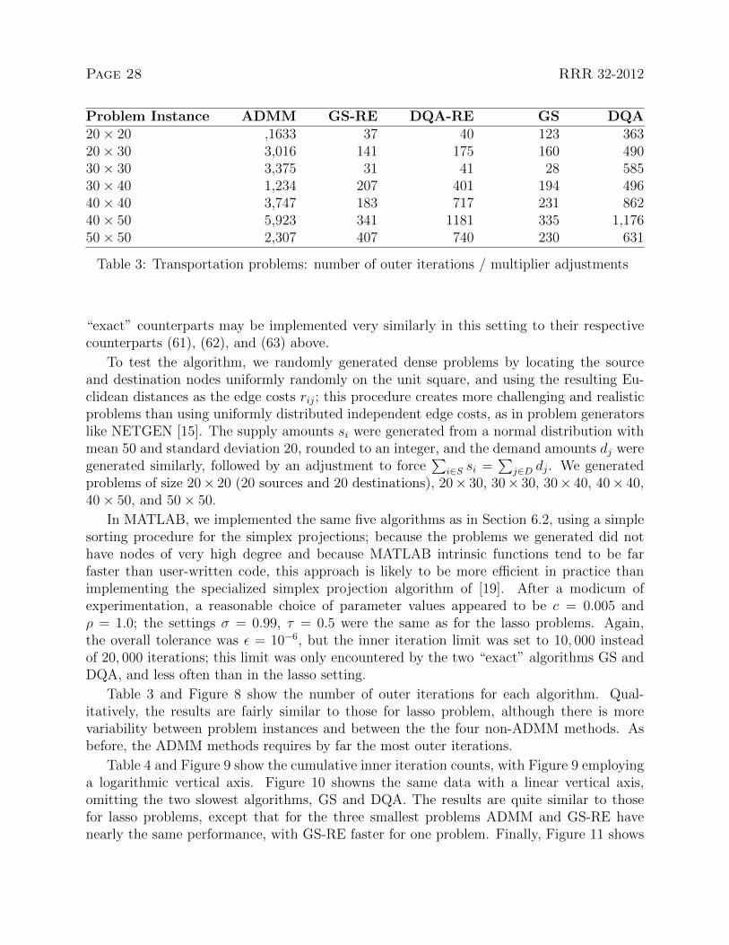
Problem Instance ADMM GS-RE DQA-RE GS DQA20× 20 ,1633 37 40 123 36320× 30 3,016 141 175 160 49030× 30 3,375 31 41 28 58530× 40 1,234 207 401 194 49640× 40 3,747 183 717 231 86240× 50 5,923 341 1181 335 1,17650× 50 2,307 407 740 230 631

Table 3: Transportation problems: number of outer iterations / multiplier adjustments

“exact” counterparts may be implemented very similarly in this setting to their respectivecounterparts (61), (62), and (63) above.

To test the algorithm, we randomly generated dense problems by locating the sourceand destination nodes uniformly randomly on the unit square, and using the resulting Eu-clidean distances as the edge costs rij; this procedure creates more challenging and realisticproblems than using uniformly distributed independent edge costs, as in problem generatorslike NETGEN [15]. The supply amounts si were generated from a normal distribution withmean 50 and standard deviation 20, rounded to an integer, and the demand amounts dj weregenerated similarly, followed by an adjustment to force

∑i∈S si =

∑j∈D dj. We generated

problems of size 20× 20 (20 sources and 20 destinations), 20× 30, 30× 30, 30× 40, 40× 40,40× 50, and 50× 50.

In MATLAB, we implemented the same five algorithms as in Section 6.2, using a simplesorting procedure for the simplex projections; because the problems we generated did nothave nodes of very high degree and because MATLAB intrinsic functions tend to be farfaster than user-written code, this approach is likely to be more efficient in practice thanimplementing the specialized simplex projection algorithm of [19]. After a modicum ofexperimentation, a reasonable choice of parameter values appeared to be c = 0.005 andρ = 1.0; the settings σ = 0.99, τ = 0.5 were the same as for the lasso problems. Again,the overall tolerance was ε = 10−6, but the inner iteration limit was set to 10, 000 insteadof 20, 000 iterations; this limit was only encountered by the two “exact” algorithms GS andDQA, and less often than in the lasso setting.

Table 3 and Figure 8 show the number of outer iterations for each algorithm. Qual-itatively, the results are fairly similar to those for lasso problem, although there is morevariability between problem instances and between the the four non-ADMM methods. Asbefore, the ADMM methods requires by far the most outer iterations.

Table 4 and Figure 9 show the cumulative inner iteration counts, with Figure 9 employinga logarithmic vertical axis. Figure 10 showns the same data with a linear vertical axis,omitting the two slowest algorithms, GS and DQA. The results are quite similar to thosefor lasso problems, except that for the three smallest problems ADMM and GS-RE havenearly the same performance, with GS-RE faster for one problem. Finally, Figure 11 shows

RRR 32-2012 Page 29

0

1000

2000

3000

4000

5000

6000

7000

20 x 20 20 x 30 30 x 30 30 x 40 40 x 40 40 x 50 50 x 50

ADMM

GS-RE

DQA-RE

GS

DQA

Figure 8: Transportation problems: number of outer iterations / multiplier adjustments

Problem Instance ADMM GS-RE DQA-RE GS DQA20× 20 1,633 1,618 5,565 12,731 39,95120× 30 3,016 3,431 11,208 24,919 74,01030× 30 3,375 2,654 7,394 26,139 81,18730× 40 1,234 2,813 7,446 26,241 76,43340× 40 3,747 9,839 19,206 111,500 247,18740× 50 5,923 8,263 27,385 212,774 486,61750× 50 2,307 13,519 41,346 152,260 311,860

Table 4: Cumulative number of inner iterations / x- or z-minimizations for transportationproblems

Page 30 RRR 32-2012

1

10

100

1,000

10,000

100,000

1,000,000

20 x 20 20 x 30 30 x 30 30 x 40 40 x 40 40 x 50 50 x 50

ADMM GS_RE DQA_RE GS DQA

Figure 9: Cumulative number of inner iterations / x- or z-minimizations for Transportationproblems

0

5,000

10,000

15,000

20,000

25,000

30,000

35,000

40,000

45,000

20 x 20 20 x 30 30 x 30 30 x 40 40 x 40 40 x 50 50 x 50

ADMM

GS_RE

DQA_RE

Figure 10: Cumulative number of inner iterations / x- or z-minimizations for tranportationproblems, omitting the GS and DQA methods

RRR 32-2012 Page 31

0

5

10

15

20

25

30

35

40

45

20 x 20 20 x 30 30 x 30 30 x 40 40 x 40 40 x 50 50 x 50

ADMM

GS_RE

DQA_RE

Figure 11: Transportation problems: run times in seconds on a Xeon X5472 3.00 GHzprocessor, omitting the GS and DQA methods

corresponding MATLAB run times on a Xeon X5472 3.00 GHz processor running UbuntuLinux 10.04. These run times closely track the inner iteration counts of Figure 10.

7 Concluding Remarks

The central point of this paper is that the ADMM algorithm, despite superficial appearances,is not simply an approximate version of the standard augmented Lagrangian method appliedto problems with a specific two-block structure. Sections 4 and 5 show that while the the-oretical convergence analysis of the two methods can be performed with similar tools, thereare fundamental differences: the convergence of standard augmented Lagrangian methodderives from a nonexpansive mapping derived from the entire dual function, whereas theADMM analysis uses the composition of two nonexpansive maps respectively obtained fromthe two additive components q1 and q2 of the dual function.

These theoretical differences are underscored by the computational results in Section 6,which compares the ADMM to both approximate and “exact” versions of the classicalaugmented Lagrangian method, using block coordinate minimization methods to (approxi-mately) optimize the augmented Lagrangian. Over two very different problem classes, theresults are fairly consistent: the ADMM makes far more multiplier adjustments then themethods derived from the classical augmented Lagrangian method, but in most cases is

Page 32 RRR 32-2012

more computationally efficient overall. In particular, the total number of iterations of theADMM is considerably less than the number of block coordinate minimization steps neededto exactly optimize even a single augmented Lagrangian. In summary, both theoretically andcomputationally, the superficially appealing notion that the ADMM is a kind of hybrid ofthe augmented Lagrangian and Gauss-Seidel block minimization algorithms is fundamentallymisleading.

It is apparent from the results for the GS and DQA algorithms that block coordinateminimization is not an efficient algorithm for minimizing the nonsmooth augmented La-grangian functions arising in either of the application classes discussed in Section 6, yet thisphenomenon does not affect the performance of the ADMM. In general, the ADMM seems asuperior algorithm to approximate minimization of augmented Lagrangians by block coordi-nate approaches; this conclusion is partially unexpected, in that the ADMM has a reputationfor fairly slow convergence, especially in the “tail”, whereas classical augmented Lagrangianmethod are generally considered competitive or near-competitive methods, and form the ba-sis for a number of state-of-the-art nonlinear optimization codes. However, the results heredo not necessarily establish the superiority of the ADMM to classical augmented Lagrangianmethods using more sophisticated methods to optimize the subproblems.

References

[1] D. P. Bertsekas. Convex Analysis and Optimization. Athena Scientific, Belmont, MA,2003. With A. Nedic and A. E. Ozdaglar.

[2] D. P. Bertsekas and J. N. Tsitsiklis. Parallel and Distributed Computation: NumericalMethods. Prentice Hall, 1989.

[3] S. Boyd, N. Parikh, E. Chu, B. Peleato, and J. Eckstein. Distributed optimization andstatistical learning via the alternating direction method of multipliers. Foundations andTrends in Machine Learning, 3(1):1–122, 2011.

[4] M. Dettling and P. Buhlmann. Finding predictive gene groups from microarray data.Journal of Multivariate Analysis, 90(1):106–131, 2004.

[5] J. Eckstein. Splitting methods for monotone operators with applications to parallel op-timization. PhD thesis, MIT, 1989.

[6] J. Eckstein. A practical general approximation criterion for methods of multipliers basedon Bregman distances. Mathematical Programming., 96(1):61–86, 2003.

[7] J. Eckstein and D. P. Bertsekas. On the Douglas-Rachford splitting method and theproximal point algorithm for maximal monotone operators. Mathematical Programming,55:293–318, 1992.

RRR 32-2012 Page 33

[8] J. Eckstein and M. C. Ferris. Operator-splitting methods for monotone affine varia-tional inequalities, with a parallel application to optimal control. INFORMS Journalon Computing, 10(2):218–235, 1998.

[9] J. Eckstein and P. J. S. Silva. A practical relative error criterion for augmented La-grangians. Mathematical Programming, 2012. Online version DOI 10.1007/s10107-012-0528-9.

[10] M. Fortin and R. Glowinski. On decomposition-coordination methods using an aug-mented Lagrangian. In M. Fortin and R. Glowinski, editors, Augmented LagrangianMethods: Applications to the Solution of Boundary-Value Problems. North-Holland:Amsterdam, 1983.

[11] D. Gabay. Applications of the method of multipliers to variational inequalities. InM. Fortin and R. Glowinski, editors, Augmented Lagrangian Methods: Applications tothe Solution of Boundary-Value Problems. North-Holland: Amsterdam, 1983.

[12] B.-S. He. Parallel splitting augmented Lagrangian methods for monotone structuredvariational inequalities. Computational Optimization and Applications, 42(2):195–212,2009.

[13] B.-S. He, Z. Peng, and X.-F. Wang. Proximal alternating direction-based contractionmethods for separable linearly constrained convex optimization. Frontiers of Mathe-matics in China, 6(1):79–114, 2011.

[14] B.-S. He, H. Yang, and S.-L. Wang. Alternating direction method with self-adaptivepenalty parameters for monotone variational inequalities. Journal of Optimization The-ory and Applications, 106(2):337–356, 2000.

[15] D. Klingman, A. Napier, and J. Stutz. Netgen: A program for generating large-scale ca-pacitated assignment, transportation, and minimum cost flow network problems. Man-agement Science, 20(5):814–821, 1974.

[16] M. A. Krasnosel’skiı. Two remarks on the method of successive approximations. UspekhiMatematicheskikh Nauk, 10(1):123–127, 1955.

[17] J. Lawrence and J. E. Spingarn. On fixed points of non-expansive piecewise isometricmappings. Proceedings of the London Mathematical Society, 3(3):605, 1987.

[18] P. L. Lions and B. Mercier. Splitting algorithms for the sum of two nonlinear operators.SIAM Journal on Numerical Analysis, 16:964–979, 1979.

[19] N. Maculan and G. G. de Paula, Jr. A linear-time median-finding algorithm for pro-jecting a vector on the simplex of Rn. Operations Research Letters, 8(4):219–222, 1989.

[20] G. J. Minty. Monotone (nonlinear) operators in Hilbert space. Duke MathematicalJournal, 29:341–346, 1962.

Page 34 RRR 32-2012

[21] R. T. Rockafellar. Convex Analysis. Princeton University Press, 1970.

[22] R. T. Rockafellar. Conjugate Duality and Optimization. SIAM, Philadelphia, 1974.

[23] R. T. Rockafellar. Augmented Lagrangians and applications of the proximal pointalgorithm in convex programming. Mathematics of Operations Research, 1(2):97–116,1976.

[24] R. T. Rockafellar. Monotone operators and the proximal point algorithm. SIAM Journalon Control and Optimization, 14(5):877–898, 1976.

[25] R. T. Rockafellar and R. J.-B. Wets. Scenarios and policy aggregation in optimizationunder uncertainty. Mathematics of Operations Research, 16(1):119–147, 1991.

[26] A. Ruszczynski. On convergence of an augmented Lagrangian decomposition methodfor sparse convex optimization. Mathematics of Operations Research, 20(3):634–656,1995.

[27] P. Tseng. Convergence of a block coordinate descent method for nondifferentiable min-imization. Journal of Optimization Theory and Applications, 109(3):475–494, 2001.