ramms 1.3.0 - slf

RAMMS 1.3.0

Rapid Mass Movements

A modeling system for snow-avalanches in research and practice

USER MANUAL v1.01

WSL Institute for Snow and

Avalanche Research SLF

March 2010

Written by

Marc Christen, Yves Buehler, Perry Bartelt and Lina Schumacher

Contents

1 Introduction 1

2 Learning by doing 3

3 Setup and First Start 5

3.1 System Requirements . . . . . . . . . . . . . . . . . . . . . . . . . . . . . . 5

3.2 Installation . . . . . . . . . . . . . . . . . . . . . . . . . . . . . . . . . . . . 5

3.2.1 Installation procedure . . . . . . . . . . . . . . . . . . . . . . . . . . 6

3.3 Licensing Methods . . . . . . . . . . . . . . . . . . . . . . . . . . . . . . . . 10

3.4 First Start . . . . . . . . . . . . . . . . . . . . . . . . . . . . . . . . . . . . . 11

3.4.1 Personal License Request File . . . . . . . . . . . . . . . . . . . . . . 11

3.4.2 Personal License Key . . . . . . . . . . . . . . . . . . . . . . . . . . . 12

3.4.3 CYGWIN / GRASS installation . . . . . . . . . . . . . . . . . . . . 13

3.4.4 Potential problem . . . . . . . . . . . . . . . . . . . . . . . . . . . . 17

3.5 Preferences . . . . . . . . . . . . . . . . . . . . . . . . . . . . . . . . . . . . 20

4 Working with RAMMS 23

4.1 General . . . . . . . . . . . . . . . . . . . . . . . . . . . . . . . . . . . . . . 23

4.1.1 Project / Scenarios . . . . . . . . . . . . . . . . . . . . . . . . . . . . 23

4.1.2 Input data . . . . . . . . . . . . . . . . . . . . . . . . . . . . . . . . 24

4.2 Model input data . . . . . . . . . . . . . . . . . . . . . . . . . . . . . . . . . 24

4.2.1 Topographic data - Digital Elevation Model . . . . . . . . . . . . . . 25

4.2.2 Forest information . . . . . . . . . . . . . . . . . . . . . . . . . . . . 25

4.2.3 Release information . . . . . . . . . . . . . . . . . . . . . . . . . . . 26

4.2.4 Global parameters . . . . . . . . . . . . . . . . . . . . . . . . . . . . 26

4.2.5 Friction information . . . . . . . . . . . . . . . . . . . . . . . . . . . 27

4.2.6 Calculation parameters . . . . . . . . . . . . . . . . . . . . . . . . . 27

4.3 The Project Wizard . . . . . . . . . . . . . . . . . . . . . . . . . . . . . . . 27

4.4 Moving, resizing and changing the view of the model . . . . . . . . . . . . . 35

4.5 Global parameters . . . . . . . . . . . . . . . . . . . . . . . . . . . . . . . . 39

4.6 Release areas . . . . . . . . . . . . . . . . . . . . . . . . . . . . . . . . . . . 40

i

Contents

4.7 Calculation Domain . . . . . . . . . . . . . . . . . . . . . . . . . . . . . . . 45

4.8 Friction parameters . . . . . . . . . . . . . . . . . . . . . . . . . . . . . . . . 46

4.9 Colorbar . . . . . . . . . . . . . . . . . . . . . . . . . . . . . . . . . . . . . . 49

4.10 Forest . . . . . . . . . . . . . . . . . . . . . . . . . . . . . . . . . . . . . . . 51

4.11 Project information . . . . . . . . . . . . . . . . . . . . . . . . . . . . . . . . 53

4.12 Changing maps and remote sensing imagery . . . . . . . . . . . . . . . . . . 55

5 Calculation and Results 57

5.1 Running a calculation . . . . . . . . . . . . . . . . . . . . . . . . . . . . . . 57

5.2 Results . . . . . . . . . . . . . . . . . . . . . . . . . . . . . . . . . . . . . . . 63

5.3 Extras . . . . . . . . . . . . . . . . . . . . . . . . . . . . . . . . . . . . . . . 69

5.3.1 Creating an image and a GIF animation . . . . . . . . . . . . . . . . 69

5.3.2 Creating a dam . . . . . . . . . . . . . . . . . . . . . . . . . . . . . . 70

5.3.3 Creating a new DEM with avalanche deposition . . . . . . . . . . . . 72

5.4 How to save input files and program settings . . . . . . . . . . . . . . . . . 73

5.5 How to open input and output files . . . . . . . . . . . . . . . . . . . . . . . 74

5.6 About RAMMS . . . . . . . . . . . . . . . . . . . . . . . . . . . . . . . . . . 75

6 Program Overview 77

6.1 The Graphical User Interface (GUI) . . . . . . . . . . . . . . . . . . . . . . 78

6.1.1 The menu bar . . . . . . . . . . . . . . . . . . . . . . . . . . . . . . . 78

6.1.2 Horizontal toolbar . . . . . . . . . . . . . . . . . . . . . . . . . . . . 89

6.1.3 Vertical toolbar . . . . . . . . . . . . . . . . . . . . . . . . . . . . . . 91

6.1.4 Main window . . . . . . . . . . . . . . . . . . . . . . . . . . . . . . . 91

6.1.5 Dump step slider . . . . . . . . . . . . . . . . . . . . . . . . . . . . . 91

6.1.6 Left status bar . . . . . . . . . . . . . . . . . . . . . . . . . . . . . . 92

6.1.7 Right status bar . . . . . . . . . . . . . . . . . . . . . . . . . . . . . 92

6.1.8 Colorbar . . . . . . . . . . . . . . . . . . . . . . . . . . . . . . . . . . 92

6.1.9 Panel . . . . . . . . . . . . . . . . . . . . . . . . . . . . . . . . . . . 92

6.2 File management . . . . . . . . . . . . . . . . . . . . . . . . . . . . . . . . . 95

6.2.1 Software RAMMS . . . . . . . . . . . . . . . . . . . . . . . . . . . . 95

6.2.2 Organizing your data . . . . . . . . . . . . . . . . . . . . . . . . . . 95

List of Figures i

List of Exercises v

ii RAMMS User Manual

1 Introduction

In the field of natural hazards there is an increasing need for process models to help un-

derstand the motion of geophysical mass movements. These models allow engineers to

predict the speed and mass of hazardous movements in complex terrain. Such models

are especially helpful when proposing mitigation measures, such as avalanche dams or

snow sheds. Hazard mapping is an especially important application in Switzerland and

other mountainous countries. While well-tested empirical methods are available to deter-

mine runout distances, velocities and flow heights, numerical models allow practitioners

to predict flow paths in general terrain as well as to model entrainment processes or the

breaking effect of forests. Numerical models have the advantage that initial and boundary

conditions can be prescribed that more exactly represent the physical problem that needs

to be solved.

RAMMS (Rapid Mass MovementS) is a state-of-the-art numerical simulation model to

calculate the motion of geophysical mass movements (snow avalanches, rockslides, debris

flows, shallow landslides) from initiation to runout in three-dimensional terrain. It was

designed to be used in practice by hazard engineers who need solutions to real, everyday

problems. It is coupled with a user-friendly visualization tool that allows users to easily

access, display and analyze simulation results. New constitutive models have been de-

veloped and implemented in RAMMS, thanks to calibration and verification at full scale

tests at sites such as Vallee de la Sionne. These models allow the application of RAMMS

to solve both large, extreme avalanche events as well as smaller mass movements such as

hillslope debris flows and shallow landslides.

RAMMS was developed by the ”Avalanche, Debris Flow and Rockfall” research unit of

the WSL Institute for Snow and Avalanche Research, SLF. This manual describes the

features of the RAMMS program - allowing beginners to get started quickly as well as

serving as a reference to expert users.

On the RAMMS web page http://ramms.slf.ch you find useful features such as a mod-

erated discussion forum, frequently asked questions (FAQ) or recent software updates.

Please visit this web page frequently to stay up to date!

1

http://ramms.slf.ch

2 Learning by doing

This manual provides an overview of RAMMS. Exercises exemplify different steps in set-

ting up and running a RAMMS simulation especially in Chapter 4: Working with

RAMMS. However, to get the most from the manual, we suggest reading it through

while simultaneously having the RAMMS program open, learning by doing. We assume

RAMMS users to have a basic level of familiarity with windows-based programs, com-

mands and general computer terminology. We do not describe the basics of windows

management (such as resizing or minimizing). RAMMS windows, click options and input

masks are similar to other windows-based programs and can be used, closed, reduced or

resized in the same way.

All topographic base maps and aerial images are reproduced c©2010 swisstopo(BA091601).

3

3 Setup and First Start

3.1 System Requirements

We recommend the following minimum system requirements for running RAMMS :

• OS: Windows XP (2000) 32 bit

• RAM (memory): 1GB (2 GB recommended)

• CPU: Intel Pentium 1 GHz (dual core recommended)

• Harddisk: ca. 410 MB

Windows Vista and Windows 7 are not supported at the moment.

3.2 Installation

Please download the RAMMS setup file ramms user setup.zip from http://ramms.slf.

ch/ramms/downloads/ramms_user_setup.zip.

Please do the following steps before you begin to install:

• Unzip the file ramms user setup.zip to a temporary directory on your target machine.

The unzipped file will be entitled similar to ramms1.3.0 user setup.exe, showing the

actual version of RAMMS (e.g. 1.3.0).

• You must have Administrator privileges on the target machine. If you do not

have such privileges, the installer cannot modify the system configuration of the

machine and the installation will fail. Note that you do not need Administrator

privileges to run RAMMS afterwards.

• Read first, install afterwards! Please read the whole installation process once, before

you begin the installation!!

5

http://ramms.slf.ch/ramms/downloads/ramms_user_setup.zip

http://ramms.slf.ch/ramms/downloads/ramms_user_setup.zip

CHAPTER 3. SETUP AND FIRST START

3.2.1 Installation procedure

Step 1: Welcome

Start the file ramms1.3.0 user setup.exe. The Welcome dialog introduces you to the En-

glish Setup program and will guide you through the installation process. Click ”Next” to

continue.

Figure 3.1: Installation - Welcome dialog window.

Step 2: Readme

Short introduction to RAMMS. Click ”Next” to continue.

Figure 3.2: Installation - Readme dialog window.

6 RAMMS User Manual

3.2. INSTALLATION

Step 3: Accepting the License Agreement

Read the license agreement carefully and accept it by activating the check box in the

lower left corner. If you do not accept the license agreement, you are not able to proceed

with the installation. After accepting the license agreement, click Next to continue the

installation.

Figure 3.3: Installation - License agreement dialog window.

Step 4: Select Destination Directory

Choose your Destination Directory. Simultaneously this dialog shows the amount of space

available on your hard disk and required for the installation. Beware: − Do NOT use a

blank or special characters within your installation directory path name (e.g.

C:\Program Files\RAMMS is not allowed, use C:\Programs\RAMMS or C:\Programme\RAMMS

instead). Click Next to start the installation process.

Figure 3.4: Installation - Destination directory dialog window.

WSL Institute for Snow and Avalanche Research SLF 7


Step 5: Installing the files

RAMMS is copying the files to the destination location and showing the installation

progress.

Figure 3.5: Installation - Installing files dialog window.

Step 6: Finished installing the files

RAMMS finished copying the files. Click Next to finish the installation process.

Figure 3.6: Installation - Finished installing files dialog window.

8 RAMMS User Manual

3.2. INSTALLATION

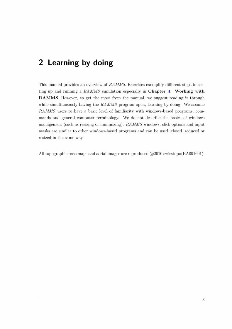
Step 7: RAMMS Installation finished!

RAMMS successfully finished the installation. Click Finish.

Figure 3.7: Installation - Finished installation dialog window.

After having successfully installed RAMMS on your personal computer, you will notice

the RAMMS icon on your desktop (for all users):

Figure 3.8: RAMMS icon.

Additionally, a new application folder is created in Start → Programs (for all users):

• RAMMS → Run RAMMS

• RAMMS → Uninstall RAMMS

Figure 3.9: RAMMS program group.



3.3 Licensing Methods

Access to RAMMS is controlled by a Personal Use License. Personal use licenses are time

limited licenses tied to a single personal computer. This method of licensing requires a

machine’s unique host ID to be incorporated into a license request file. After the license

request file is sent to WSL/SLF, you will receive a license key. Entering the license key on

a personal computer enables full RAMMS functionality for the specific personal computer.

For more information please visit http://ramms.slf.ch.

10 RAMMS User Manual

http://ramms.slf.ch

3.4. FIRST START

3.4 First Start

Double-click the icon or use Start → Programs → RAMMS → Run RAMMS to start

RAMMS for the first time. Whenever you start RAMMS, the splash screen below will

pop up:

Figure 3.10: RAMMS start window.

Click on the image. It will disappear and RAMMS will start up. The following dialog

window appears (Fig. 3.11 RAMMS - Licensing):

Figure 3.11: RAMMS licensing window.

3.4.1 Personal License Request File

Click the button to create your personal license request file. In Fig. 3.12 enter your

full name and the name of your company.

In the next dialogue window, choose the destination directory of your personal license

request file and save it to your target machine. Your personal license request file should

look similar to Fig. 3.13.



Figure 3.12: Enter user name and company name.

Figure 3.13: Personal license request file RAMMS request Muster Test.txt

3.4.2 Personal License Key

How to order a Personal License Key

You find an order form on the RAMMS web page at http://ramms.slf.ch/. Fill in all

your personal information, choose license period, license typ and number of licenses you

wish to order, attach your personal license request file, accept the license agreement and

click Submit Order.

An order confirmation email is sent to your Email address. We then process your order

and send you an invoice. As soon as we received your payment, we will send you your

personal license key. Your personal license key is named similar to RAMMS license Muster

Test.txt. Open the file in a text-editor. It should look similar to Fig. 3.14.

Now, restart RAMMS (as explained before). Again, the pop-up window (Fig. 3.10) and

then the dialogue window of Fig. 3.11 appears (RAMMS - Licensing).

Copy the license key (in this example: akck-3ijh-3jtl-2h5h-g340 ) and paste it at LICENSE

KEY: (see Figure 3.11). If RAMMS accepts your installation key, you successfully finished


http://ramms.slf.ch/

3.4. FIRST START

Figure 3.14: Personal license key file RAMMS license Muster Test.txt

the installation. Please continue with section 3.4.3 and install Cygwin/GRASS (required

to use RAMMS ).

3.4.3 CYGWIN / GRASS installation

RAMMS is coupled to the Open Source GIS Software GRASS . Before you can benefit of

all the functions of RAMMS, you must install GRASS on your PC. RAMMS works with

GRASS version 6.2.3. Later versions of GRASS are not supported in RAMMS. GRASS

needs Cygwin, a Linux-like environment for Windows. Please perform the following steps

to install both GRASS and Cygwin:

• Be aware: You need Administrator privileges on the target machine to install

GRASS !

• Run Track → Install Cygwin/GRASS to install GRASS Version 6.2.3 .

Figure 3.15: Continue Cygwin/GRASS installation?

Click YES to begin the installation of Cygwin and GRASS.


http://grass.itc.it/intro/general.php


• Choose the file Cygwin623.zip in the Temp-directory of your RAMMS -distribution

and click OK.

Figure 3.16: Choose Cygwin/GRASS installation zip-file.


3.4. FIRST START

• In the next window you are asked to specify the installation directory. Choose

e.g. C:\Programs without cygwin, because cygwin will be appended automatically!

VERY IMPORTANT: Do NOT use BLANKS or any special characters

in the installation path!!

Figure 3.17: Choose Cygwin/GRASS installation directory.



• The files are now being extracted to the directory you specified before. Please be

patient, because this can take a while!

Figure 3.18: Cygwin/GRASS - Extract files.

• To finish our installation of Cygwin/GRASS, we have to update the Windows reg-

istry with the Cygwin/GRASS information. Click YES in the window below:

Figure 3.19: Cygwin/GRASS - Add to registry.

Figure 3.20: Cygwin/GRASS - Registered successfully.


3.4. FIRST START

• At the end a few Cygwin/GRASS scripts are executed. The installation of Cyg-

win/GRASS is now completed!

Figure 3.21: Cygwin/GRASS - Automatic scripts.

3.4.4 Potential problem

The following error can occur:

Figure 3.22: Error message

This error occurs, if certain .NET libraries are missing on your target machine. You

need to install these missing libraries. Start the installer by double-clicking the file

run system32 dll.bat in the Temp folder of your RAMMS installation directory. Follow

the instructions below to install the files:



Step 1: Welcome to IDL Visual Studio Merge Modules

The Welcome dialog introduces you to the English Setup program and will guide you

through the installation process of the IDL Visual Studio Merge Modules. Click ”Next”

to continue.

Figure 3.23: IDL Visual Studio Merge Modules - Welcome dialog window.

Step 2: Ready to install the Program

Click ”Next” to continue.

Figure 3.24: IDL Visual Studio Merge Modules - Ready to install the Program.


3.4. FIRST START

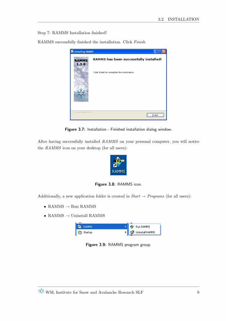
Step 3: Installing IDL Visual Studio Merge Modules

The wizard is installing the files. Please wait until it is finished.

Figure 3.25: IDL Visual Studio Merge Modules - Installing...

Step 4: InstallShield Wizard Completed

The wizard completed the installation. Click Finish.

Figure 3.26: Installation - Destination directory dialog window.

You successfully installed the necessary files and RAMMS should start now normally. Go

back to section 3.4 and start RAMMS.



3.5 Preferences

Before starting to work with RAMMS, be sure to set your RAMMS preferences and place

the necessary DEM (Digital Elevation Model) files as well as the FOREST files, MAPS

and georeferenced IMAGERY you wish to use in the appropriate folders defined in the

preferences, see Figs. 3.27 and 3.28.

Use Track → Preferences to open the RAMMS preferences window or click the

button .

• General tab

Setting Purpose

Cygwin directory

This field allows you to set the Cygwin directory.

This should correspond to your installation di-

rectory of Cygwin, e.g. C:\Programme\cygwin.

GRASS version

Use this field to specify the GRASS version you

use. You can find your current GRASS version

here: C:\Programme\cygwin\usr\local\grass-

6.X.X (default grass-6.2.3).

Working directory

Set your working directory. VERY IMPOR-

TANT: Do NOT use BLANKS in the work-

ing directory path!!

Map directory

Set the folder where you place your georefer-

enced digital maps (consists of a TIFF-file and

a corresponding tfw-file (world-file).

Image directory

Set the folder where you place your digital

georeferenced orthophotos (aerial picture, con-

sists of a TIFF-file and a corresponding tfw-file

(world-file).

DEM directory

Set the folder where you place the Digital

Elevation Models (format: ASCII grid, see 4.2.1

on page 25)

FOREST directorySet the folder where you place your forest-files

(formats: ASCII grid or polygon shapefile).


3.5. PREFERENCES

• Avalanche tab

Setting Purpose

Read timestepsChoose between reading ALL or only 1 timestep.

Default is reading ALL timesteps.

Nr of colorbar colors Set default nr of colorbar colors.

GIF-Animation interval (s) Set interval for GIF-Animation images.

Background colorSet background color (greyscale between 0:black

and 255:white).

Animation delay (s)Set animation delay to decelerate the animation

speed.

Figure 3.27: General tab of RAMMS

preferences.

Figure 3.28: Avalanche tab of

RAMMS preferences.

See exercise ”Working directory” on page 22 below on how to choose a new working

directory. All further settings can be changed in a similar manner. The settings are saved,

until they are changed again manually.



Exercise 3.5.a: Working directory

Choosing the right working directory is very useful and saves a lot of time, searching

for files and folders.

◦ Click (or use Track → Preferences) to open the RAMMS preferences

window.

◦ Click into the field Working directory, then the appearing arrow and Edit...

A window pops up where you can choose your new working directory. Click

OK in both windows.

Figure 3.29: RAMMS preferences.Figure 3.30: Browse for the correct

folder.

End of Example 3.5.a


4 Working with RAMMS

4.1 General

To successfully start a new RAMMS project, a few important preparations are necessary.

Topographic input data (ascii format), project boundary coordinates and georeferenced

maps or remote sensing imagery should be prepared in advance (.tif format and .tfw file,

maps and imagery are not mandatory, but nice to have). Georeferenced datasets have to

be in a Cartesian coordinate system (e.g. Swiss CH1903+ LV95), polar coordinate systems

(e.g. WGS84 Long Lat) are not supported. Fore more information about specific national

coordinate systems please contact the national topographic agency.

4.1.1 Project / Scenarios

A project is defined for a region of interest. Within a project, one or more scenarios

can be specified and analyzed. For every scenario, a calculation can be executed. A

project consists therefore of different scenarios (input files) with different input parameter

files (release and friction files). The basic topographic input data is the same for every

scenario. If you want to change the topographic input data (e.g. change the input DEM

resolution or the project boundary coordinates) you have to create a new project. Other

input parameters (like friction parameters, release areas, calculation domain, calculation

grid resolution, end time, time step etc.) can be changed for every scenario.

23

CHAPTER 4. WORKING WITH RAMMS

Figure 4.1: Project extent (area of interest) - topographic map c©2010 Swisstopo

(BA091601).

4.1.2 Input data

There are different kind of data to be provided to successfully perform a calculation with

RAMMS. Topographic data, definition of release area and release mass as well as infor-

mation about friction parameters are mandatory.

RAMMS is able to process (see Figs. 4.2 and 4.3)

• ESRI ASCII Grid and

• ASCII X,Y,Z single space data.

These data types are also available e.g. from www.swisstopo.ch. Because RAMMS needs

the topographic data as an ESRI ASCII Grid, ASCII X,Y,Z data can be converted within

RAMMS into an ESRI ASCII Grid.

4.2 Model input data


4.2. MODEL INPUT DATA

4.2.1 Topographic data - Digital Elevation Model

The topographic data is the most important input requirement. The simulation results

depend strongly on the resolution and accuracy of the topographic input data. The to-

pographic data MUST be provided as an ESRI ASCII Grid. No other type is allowed

at the moment. The user must therefore prepare the topographic data according to this

limitation. The header of an ESRI ASCII Grid must contain the information shown in

Fig. 4.2

Figure 4.2: Example ESRI ASCII Grid.

An ESRI ASCII GRID can be created in ArcGIS with the function ArcToolbox→Conversion

Tools→From Raster→Raster to ASCII.

It is possible to import ASCII X,Y,Z single space data and convert the data into an ESRI

ASCII Grid (using Track→New...→Convert XYZ to ASCII Grid).

4.2.2 Forest information

Forest information is not required for a successfull simulation, but recommended, because

the friction parameters depend strongly on forest information. Forest information can be

provided as:

• ESRI ASCII GRID (0: no forest, 1: forest)

• Polygon shapefile



Figure 4.3: Example ASCII X,Y,Z single space data.

If no such files are available, the user can draw a polygon shapefile in RAMMS and import

it as forest information (see section 4.10 on page 51).

4.2.3 Release information

The definition of release areas and release heights have a very strong impact on the results

of RAMMS simulations. Therefore we recommend to use reference information such as

photography, GPS measurements or filed maps to draw release areas. This should be done

by people with experience concerning the topographic and meteorological situation of the

investigation area.

Users have to draw their own release polygon shapefiles, see section 4.6 on page 40. All

release informations are saved as polygon shapefiles and can be easily imported in GIS-

Software (e.g. ArcGIS). Shapefiles created in e.g. ArcGIS can be imported into RAMMS

by using GIS/GRASS → Convert Shapefile... → Polygon Shapefile to RAMMS Release

Shapefile.

4.2.4 Global parameters

The two global parameters return period and avalanche volume category influence the

classification of the friction information.


4.3. THE PROJECT WIZARD

4.2.5 Friction information

An automatic RAMMS procedure calculates friction values based on topographic data

analysis (slope angle, altitude and curvature), forest information and global parameters,

see section 4.8 on page 46. All friction informations are saved as polygon shapefiles and

can be easily imported in GIS-Software (e.g. ArcGIS).

4.2.6 Calculation parameters

Calculation parameters such as output name, simulation grid resolution, end time, time

step etc. can be changed interactively in RAMMS.

4.3 The Project Wizard

A new project is created with the RAMMS Project Wizard, shown in the exercise below.

The wizard consists of four steps:



Exercise 4.3.a: How to create a new project.

◦ Click or Track ⇒ New ⇒ Project wizard to open the RAMMS Project

Wizard.

◦ The following window pops up:

Figure 4.4: RAMMS Avalanche Project Wizard: Step 1 of 4.



Step 1:

◦ Enter a project name (1).

◦ Add some project details (2).

◦ The project location (3) suggested is the current working directory. To change

the location click into the location field. A second window appears and you can

browse for a different folder (see figure below, VERY IMPORTANT: Do NOT

use BLANKS or special characters in the project location path!).

◦ Click Next (4).

Figure 4.5: Step 1 of the RAMMS

project wizard: Project information.

Figure 4.6: Window to browse for a

new project location.

Step 2:

◦ Locate your DEM- and FOREST-file

in the folder set in the RAMMS pref-

erences. Click into the corresponding

fields to browse for the appropriate files

(1).

◦ If you don’t want to use a FOREST-

file, select ”Do NOT use forest infor-

mation” (2).

◦ Click Next (3).

Figure 4.7: Step 2 of the

RAMMS project wizard: GIS

information.



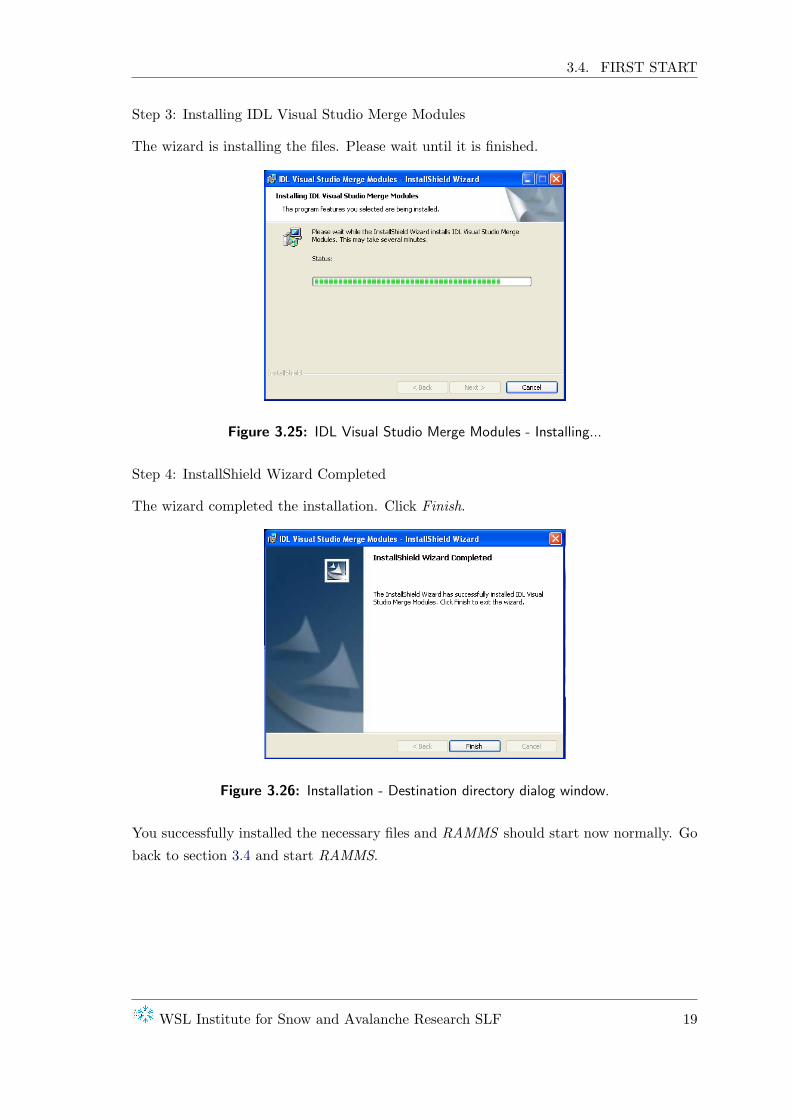
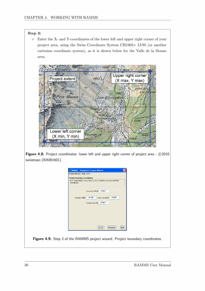
Step 3:

◦ Enter the X- and Y-coordinates of the lower left and upper right corner of your

project area, using the Swiss Coordinate System CH1903+ LV95 (or another

cartesian coordinate system), as it is shown below for the Valle de la Sionne

area.

Figure 4.8: Project coordinates: lower left and upper right corner of project area - c©2010

swisstopo (BA091601).

Figure 4.9: Step 3 of the RAMMS project wizard: Project boundary coordinates.



Step 4:

◦ Check the project summary,

especially if a DEM- and

FOREST-file was found.

◦ To make changes click Pre-

vious, to create the project

click Create Project Ex-

ample1.

Figure 4.10: Step 4 of the RAMMS project

wizard: Project summary.

End of exercise 4.3.a



The creation process can take a while. Different status bars will pop up and show the

progress of the project creation process, see table below:

Progress bar Purpose

GRASS function: Import the

DEM file

GRASS function: Import the

FOREST file and export the

file forest5m.asc

GRASS function: Export the

file Example1.xyz with the to-

pographic data

Reading topographic data (x-,

y- and z-coordinates).

Analysing the topography

and calculating curvature and

slope angles

Preparing topography for dis-

playing in RAMMS

Searching georeferenced maps

in the Maps-Folder



If more than one map was

found, the user can select a

map

If the map is much bigger

than the project-region, the

user can crop the map to im-

prove the quality of the map-

visualization

Searching georeferenced maps

in the Orthophoto-Folder

If no image was found, the

user can specify another folder

or abort the process



The following files will be created in the project-folder

Figure 4.11: Created project files.

File / Folder Purpose

doc (folder) Folder containing input and ouput LOG files

grassloc (folder)Folder containing GRASS files: do NOT delete

or change them

logfiles (folder) Log-files for GRASS operations

shell (folder) Folder containing GRASS shell scripts

.grassrc6 GRASS ini file: do NOT delete or change

dhm.asc ASCII Grid with altitude values

Example1.av2 Input file

Example1.dom Calculation domain ASCII file

Example1 dom.shp Calculation domain shapefile

Example1 dom.shx Calculation domain shapefile

Example1 dom.dbf Calculation domain shapefile

Example1.xyz Topographic data used in RAMMS

forest shp.shp Extracted forest shapefile

forest shp.shx Extracted forest shapefile

forest shp.dbf Extracted forest shapefile


4.4. MOVING, RESIZING AND CHANGING THE VIEW OF THE MODEL

forest5m.ascASCII Grid with forest information (0:no forest,

1:forest)

4.4 Moving, resizing and changing the view of the model

Once the project is created, there are several useful tools that might be helpful when

working with RAMMS. They are explained in the excercises below.



Exercise 4.4.a: Moving and resizing the model

a) Terrain model has a dimension of 100% or smaller:

◦ By clicking on the ”arrow” , the model can be moved and resized.

Figure 4.12: ”Active” project with lines and corners for resizing, topographic map c©2010

Swisstopo (BA091601)

◦ To move the model without changing size or aspect ratio, move to the model

and check if the cursor turns to . Then click and hold the left mouse button

and drag the model to the desired position.

◦ To resize the model without changing the aspect ratio, move to one of the green

corners. If the cursor turns to , click and hold the left mouse button. By

moving the mouse towards the model, the size will be reduced (move away to

enlarge the model). Alternatively you can resize the model by changing the

percentage value in the horizontal toolbar .


4.4. MOVING, RESIZING AND CHANGING THE VIEW OF THE MODEL

◦ To resize the model by changing the aspect ratio, go on one of the green lines.

When the mouse cursor changes to , click and hold the left mouse button

and change the size by moving the mouse.

b) Terrain model has a dimension > 100%:

◦ All steps explained above are still possible. Especially for the last two steps

explained, the view of one of the corners or lines is required.

◦ In addition to this, the white hand right next to the rotation button becomes

active as well. After clicking on this so-called ”view pan” button , it

is also possible to move the model.


Exercise 4.4.b: Rotating the model

◦ After activating the rotation button , the model can be rotated along

the rotation axis, by moving the cursor directly on one of the axis until the

cursor changes from to . Otherwise a freehand rotation in any direction

is possible.

Figure 4.13: ”Active” project with rotation axes, topographic map c©2010 swisstopo

(BA091601).

End of exercise 4.4.b



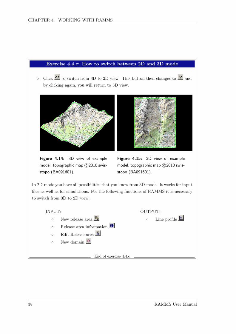
Exercise 4.4.c: How to switch between 2D and 3D mode

◦ Click to switch from 3D to 2D view. This button then changes to and

by clicking again, you will return to 3D view.

Figure 4.14: 3D view of example

model, topographic map c©2010 swis-

stopo (BA091601).

Figure 4.15: 2D view of example

model, topographic map c©2010 swis-

stopo (BA091601).

In 2D-mode you have all possibilities that you know from 3D-mode. It works for input

files as well as for simulations. For the following functions of RAMMS it is necessary

to switch from 3D to 2D view:

INPUT: OUTPUT:

◦ New release area ◦ Line profile

◦ Release area information

◦ Edit Release area

◦ New domain

End of exercise 4.4.c


4.5. GLOBAL PARAMETERS

4.5 Global parameters

Figure 4.16: RAMMS global parameters.

Prior to creating a new muxi-file, choose the return period and the volume category. The

MuXi-file will be calculated based on these values. Changing the return period and/or

volume category has no effect on already existing muxi-files. The default volume category

is chosen based on the specified release volume.



4.6 Release areas

There are different possibilities to include a release area into the project. This is of course

necessary to run a calculation. The following table gives an overview of the possibilities

RAMMS offers. For further explanations see the exercises below.

Create a new release area

If there is no release area available for your project, or

you wish to create a new one, switch to 2D mode and

click .

Load an existing release

area

Load an existing release area with Input ⇒ Release

area ⇒ Load existing release area.

Import a shapefile and con-

vert it to a release area

Draw a release area using a GIS-tool and save it as

shapefile (.shp). Then convert the shapefile using

GIS/GRASS ⇒ Convert Shapefile ⇒ Polygon

Shapefile to RAMMS Release Shapefile.

The defnition of release areas and release heights have a very strong impact on the results

of RAMMS simulations. Therefore we recommend to use reference information such as

photography, GPS measurements or filed maps to draw release areas. This should be done

by people with experience concerning the topographic and meteorological situation of the

investigation area.


4.6. RELEASE AREAS

Exercise 4.6.a: How to create a new release area.

◦ Switch to 2D mode by clicking .

◦ Activate the project by clicking on it once.

◦ Click .

◦ Click into the project where you want to start drawing the outline of the release

polygon.

◦ Continue drawing the release polygon by moving the cursor and clicking the

left mouse button.

◦ To end the release polygon, double-click the left mouse button. The polygon

will be closed automatically.

Figure 4.17: Project with emerging release area.

Before the release area is created, you have to answer a few questions:

◦ Add more release areas?

You can either answer with Yes and create a second release polygon as explained

above or answer with No and continue with the next step.

◦ Choose a new release filename:

Enter a new name for the release area. The ending *rep.shp is added automat-

ically.

The release area will now be created and opened directly, as well as the colorbar.




Exercise 4.6.b: How to load an existing release area.

◦ Choose Input→Release area→Load existing release area.

◦ Select release file (*rep.shp) and click open.

⇒ The release area appears in the project as well as the colorbar for the variable

release height (m)



4.6. RELEASE AREAS

Once a release area is created or loaded, you have to specify the release height. Choose

Input→Release Area...→View and Edit Release Areas or click the button and

choose the release area polygon by selecting it with the left mouse button. The appear-

ing window yields information about release area, mean slope angle, mean altitude and

estimated release volume. And, most importantly, the release height can be entered, see

exercise below.

Additional release information is found in the avalanche panel in the volumes-tab, see

Figure below.

Figure 4.18: Release area and volume information.



Exercise 4.6.c: Specify release height and view release information

◦ Switch into 2D mode by clicking .

◦ Click on the ”View and Edit Release Information” button (in the hori-

zontal toolbar or in the Volumes-tab in the panel) or choose Input→Release

Area...→View and Edit Release Areas.

◦ Then click on the release area you want to get information on. A red polygon

is drawn around the selected release area. The following window appears:

Figure 4.19: Release area information window.

Remark: The estimated release volume shown is estimated, calculated with a mean

slope angle for the whole release area.

◦ To change the release height enter a new value (the resulting release volume is

directly adjusted. Click OK if you want to keep the changes, Cancel otherwise.



4.7. CALCULATION DOMAIN

4.7 Calculation Domain

To save calculation time you can specify a calculation domain. If you know where the

avalanche path is situated (e.g. by running a calculation with a coarse cell size, e.g. 25m),

you can exclude the area which is not of interest. Switch to 2D mode and chose Input

→ Calculation Domain... → Draw new Domain. Now you can draw a polygon con-

taining the area of interest accordingly to drawing a new release area (see exercise ”Create

release area” on page 40). We strongly recommend to use Calculation Domains especially

if you calculate with small cell sizes (e.g. < 5m).

Figure 4.20: Calculation domain in green confines the area of interest and saves calculation

time.



4.8 Friction parameters

RAMMS employs a Voellmy-fluid friction model. This model divides the frictional re-

sistance into two parts: a dry-Coulomb type friction (coefficient µ) that scales with the

normal stress and a velocity squared drag (coefficient ξ). The frictional resistance S (Pa)

is then

Figure 4.21: RAMMS Voellmy-fluid friction model.

where ρ is the flow density, g gravitational acceleration, φ the slope angle, H the flow

height and U the flow velocity. This model has found wide application in the simulation

of mass movements, especially snow avalanches. The Voellmy model has been in use in

Switzerland for a long time and a set of calibrated parameters is available.

RAMMS offers a constant and a variable calucation mode. If a calculation is done with

constant friction values, of course, no terrain undulations and forest areas are considered.

Therefore we suggest to use the variable friction values if possible. µ and ξ depend

strongly on the global parameters return period and avalanche volume. Therefore, you

MUST define an appropriate return period and check your avalanche volume in the Global

Parameters (Input→Global Parameters) BEFORE creating a new MuXi file!


4.8. FRICTION PARAMETERS

Figure 4.22: RAMMS — Automatic MuXi Procedure.

How to create a new MuXi file is demonstrated in the exercise ”How to create a new MuXi

file” on page 47 below.

Before running a calculation, make sure you chose variable friction parameters if you want

to take the topography into account (Mu/Xi tab in the Run calculation window).

In case you closed and then reopened a project and did not save it with the created MuXi

file, you can simply load the MuXi file again and do not have to create it again (see exercise

”How to load an existing MuXi file” on page 47).



Exercise 4.8.a: How to create a new MuXi file.

◦ Choose Input→Friction Values...→Create new MuXi file (Automatic

Procedure).

◦ Enter a file name.

◦ Unless you know better, leave the values as they are...

◦ Click OK.

◦ The MuXi file will be loaded after it is created. If you create the first MuXi file

for this project, this procedure can take a while, depending on your computer’s

performance (CPU and RAM). The creation of following MuXi files will be

much faster.

◦ You can switch between the release area (if already loaded), the Mu and Xi

value via the avalanche panel.


Exercise 4.8.b: How to load an existing MuXi file.

◦ Choose Input→Friction values→Load existing MuXi file.

◦ A window opens to browse for an existing MuXi file (*MuXi.shp)

◦ Click Open and the file will be loaded.



4.9. COLORBAR

4.9 Colorbar

As soon as a parameter is shown in the project, the colorbar appears on the right side of

the main window. It can be turned on and off by clicking on .

Exercise 4.9.a: Editing the colorbar

Changing the min and max values of the colorbar as well as changing the number of

colors used is done in the Avalanche Panel under Display.

◦ Simply type a new value into the re-

spective field and hit the return key

on the keyboard. The display will

be refreshed.

◦ A further, very helpful thing to

change is the transparency. This is

useful when the topography should

be visible through the avalanche.

◦ ATTENTION: The line Values <

x.xxx are not displayed!! is im-

portant. Depending on your min

and max values, check this line to

know, which values are not dis-

played! Figure 4.23: The avalanche ’Display’

panel.



◦ Open the editing window by either choosing

Edit→Edit colorbar properties (only

INPUT) or clicking in the vertical tool-

bar.

◦ To change the colorbar properties simply

click into the field you want to change, then

click OK.

Figure 4.24: The colorbar prop-

erties window.



4.10. FOREST

4.10 Forest

It is necessary to take forest areas into account, when running a simulation with variable

friction parameters (Mu and Xi).

The easiest way to consider forest, is to have a digital forest file (ASCII grid or forest

shapefile) located in the folder set in the RAMMS preferences (FOREST directory). In

this case the forest file will already be included while creating the project. Step 2 of the

RAMMS::Avalanche Project Wizard deals with the DEM- and FOREST-files. Click into

the field once, to browse for your FOREST-file.

If you have a forest-file available and located in the FOREST folder but don’t want to use

it, click ”Do NOT use forest information”. This is necessary, e.g., if you want to simulate

a situation without considering the forest.



Exercise 4.10.a: How to create a FOREST file.


◦ Activate project by clicking on the map once.

◦ Click or choose Input→Forest...→Draw New Forest Areas.

◦ Trace the forest outline by creating as many FOREST area polygons as nec-

essary (proceed as in exercise ”How to create a new release area” on page 40)

and name your new FOREST file. A new FOREST shapefile is saved.

◦ You are asked, if you want to import the created FOREST file into your project.

Click YES, if you want to use the newly created FOREST (ignore the next

point in this case). Otherwise click NO and import the FOREST file later, as

explained in the next point.

◦ Import the new FOREST shapefile: Choose Input→Forest...→Import For-

est Area From SHAPEFILE, then select your FOREST shapefile.

◦ This new FOREST information is not automatically taken over in existing

MuXi-files. Therefore, recreate existing MuXi-files if needed. If you create

a new MuXi file with Input→Friction Values...→Create new MuXi file

(Automatic Procedure), the forest will now be considered.



4.11. PROJECT INFORMATION

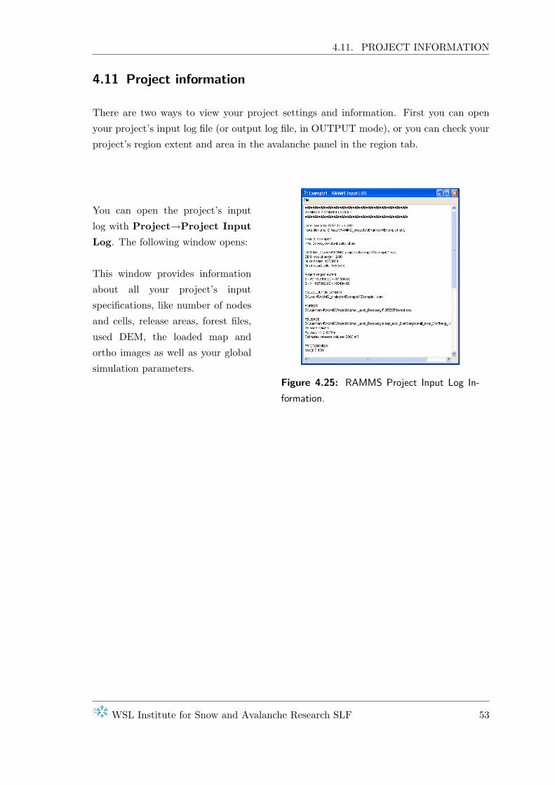
4.11 Project information

There are two ways to view your project settings and information. First you can open

your project’s input log file (or output log file, in OUTPUT mode), or you can check your

project’s region extent and area in the avalanche panel in the region tab.

You can open the project’s input

log with Project→Project Input

Log. The following window opens:

This window provides information

about all your project’s input

specifications, like number of nodes

and cells, release areas, forest files,

used DEM, the loaded map and

ortho images as well as your global

simulation parameters.Figure 4.25: RAMMS Project Input Log In-

formation.



Figure 4.26: Region extent (X-, Y- and

Z-Coordinates, total area).

To view the project coordinates, click the

region tab in your avalanche panel. The

region tab lists X- and Y-Coordinates

of the lower left (min values) and upper

right (max values) corner (this are the

coordinates you entered when creating the

project) as well as the global minimum

and maximum of altitude (Z value). The

X- and Y-Coordinates do not correspond

exactly to the clipping values you entered

at creation time of the project. This is

due to the clipping algorithm in GRASS.

Additionally, the total region area is

shown (in km2).


4.12. CHANGING MAPS AND REMOTE SENSING IMAGERY

4.12 Changing maps and remote sensing imagery

It is possible to change the map or imagery of a project anytime. Take into account, that

the corresponding TFW-file (world-file) has to be in the same folder as the actual map

(*.tif). If this is not the case, the map will not be found!

Exercise 4.12.a: How to add or change maps.

◦ Go to Extras→Add/Change Map.

If more than one map is found, the following window pops up, listing the maps

found:

Figure 4.27: Window to choose map image.

Information on the image dimensions (x-Dim and y-Dim, pixel) and size (in

MB) are provided and might be a selection criterion.

◦ Select the map you wish to add and click Load selected map.

◦ If the question ”No map found, continue search?” appears, you either don’t

have an appropriate map, the Map-folder directory is set wrong or the map is

saved in a different folder. In the latter case click Yes and choose the correct

folder.

◦ Click No to cancel search.

◦ Click Yes to continue search.

◦ A window pops up to browse for the correct map location and file.



◦ If the question ”Map area is much larger than your region! Do you wish to crop

the map?” appears, as it says, your map is much larger than your project area.

◦ Click No to load the map without croping. It may lead to a bad resolution.

◦ We suggest to click Yes. The map will be cropped to the same size as the

project region. A window opens to enter a name for the new map. The default

saving location is the one set in the RAMMS preferences. You can change it if

necessary.


Exercise 4.12.b: How to add or change remote sensing imagery.

◦ Go to Extras→Add/Change image.

See exercise ”How to add and change maps” on page 55 above.


To check which map and imagery are currently loaded in the project, open the project

input (or output) log (Project→Project Input Log. Next to ”Map image:” and ”Ortho

image:” you will find the location and name of the loaded map and imagery, respectively.


5 Calculation and Results

5.1 Running a calculation

To run a calculation one has to have created a project, loaded a release area and if a cal-

culation with variable friction parameters is desired, a muxi-file must have been created as

well. Below you find two short examples, one for running a constant calculation (constant

release height and constant friction parameters µ and ξ) and one for using variable release

height and friction parameters.

57

CHAPTER 5. CALCULATION AND RESULTS

Exercise 5.1.a: How to run a constant avalanche calculation.

◦ To run a calculation choose Run→Run Avalanche Calculation or click .

◦ The RAMMS::Input Parameters window opens.

◦ Before clicking RUN CALCULATION, you should check the input param-

eters.

◦ General:

(1) Project name

(2) Project infos. You can change

them by simply typing into

the field.

(3) Additional information: Cal-

culation domain file and DEM

file.

(4) Select an output filename.Figure 5.1: General information.


5.1. RUNNING A CALCULATION

◦ Params:

(1) Change grid resolution, if nec-

essary.

(2) Choose end time of simula-

tion.

(3) Choose dump step interval.

(4) Keep the default value for

density.

(5) Change numerical solver, 1st

or 2nd order scheme (we rec-

ommend 2nd order).Figure 5.2: Calculation parame-

ters

◦ Mu/Xi:

(1) For a calculation with con-

stant MuXi-values, click con-

stant.

(2) Enter Mu and Xi values.

Choose Help→RAMMS

Manuals...→Friction Pa-

rameter Table (PDF) or

see friction value table in the

appendix for an idea of µ and

ξ! Figure 5.3: Friction values MuXi.

◦ Release:

(1) The text field should indicate

your release shapefile.

(2) The estimated release volume

is stated in the second text

field.

Figure 5.4: Release information.WSL Institute for Snow and Avalanche Research SLF 59


◦ Stop:

(1) The stopping criteria in

RAMMS is based on the

momentum. In classical

mechanics, momentum (SI

unit kgm/s, or, equivalently,

Ns) is the product of the mass

and velocity of an object (p

= mv). For every DUMP

STEP, we sum the momenta

of all grid cells, and compare

it with the maximum momen-

tum sum. If this percentage

is lower than a user defined

threshold value (see below),

the program is interrupted

and the avalanche is re-

garded as stopped. Threshold

values between 1-10% are

reasonable, but this is only

a suggestion and must be

validated by the individual

user himself.

Figure 5.5: Stop criteria.


5.1. RUNNING A CALCULATION

◦ Click RUN CALCULATION (fig. 5.4).

◦ The following window appears, showing the status of the calculation.

Figure 5.6: Status window of calculation.

◦ Once it’s finished, the simulation is opened in RAMMS.

Figure 5.7: Main window in output mode, topographic map c©2010 Swisstopo (BA091601).




Exercise 5.1.b: How to run a variable avalanche calculation.

The process for a variable calculation is almost the same than for a constant calcula-

tion! Therefor this exercise only shows the difference to the exercise above (exercise

”How to run a constant avalanche calculation” on page 57).

◦ Mu/Xi:

(1) For a calculation with variable

MuXi-values, click variable.

(2) Check, if the correct MuXi-file

is used.

If a different file should be

used, click into the field and

browse for the desired file.Figure 5.8: MuXi settings for a variable

calculation.



5.2. RESULTS

5.2 Results

This section just gives a short overview on what is possible to do with the simulation

results. The interpretation of the results has to be done by an avalanche expert who is

familiar with the topographic and meteorological situation of the investigation area. The

RAMMS simulation results should not be used without questioning them! Perform sensi-

tivity studies!

The drop down menu Results offers the following functions:

• Flow Height

• Flow Velocity

• Flow Pressure

• Flow Momentum

• Max values (Height, Velocity, Pressure, Momentum)

• DEM Adaptations (Add Deposition to DEM)

• Flow Analysis (Summary of Moving Mass)

• Friction Values (Mu, Xi)

These results are all visualized by a colorplot in the topography. See exercise ”Displaying

max values” on page 64.

In the horizontal toolbar you find two further functions:

• Line Profile

• Time plot

Line profile

A line profile is a good alternative to the color plot, if the avalanche snow height, velocity

or pressure should be known at a specific location. The graph shows the currently active

parameter. Every line profile is saved in the file profile.txt in the project directory. If

you want to keep this line profile, you have to save it, see exercise ”How to draw a line

profile” on page 64.



Time plot

This function provides a time plot at a single point. This is helpful, when knowing the

position of an obstacle (building, dam, tree...) and the (max) values at this location over

time are a relevant information. Every point is saved in the file point.txt and a point-

info file point info.txt is additionally saved in the project directory. If you want to keep

this point, you have to save it, see exercise ”How to create a timeplot” on page 64. The

point-info file can be visualized with Extras→Point...→View Point Info File.

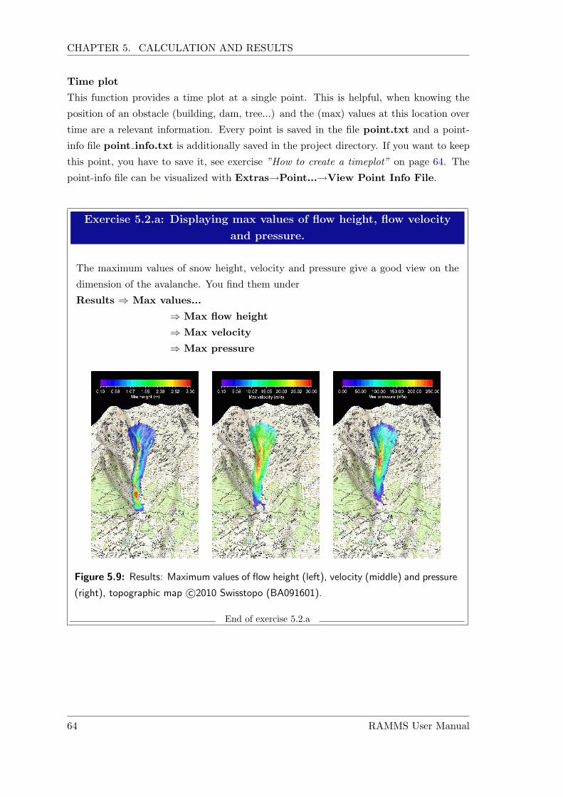
Exercise 5.2.a: Displaying max values of flow height, flow velocity

and pressure.

The maximum values of snow height, velocity and pressure give a good view on the

dimension of the avalanche. You find them under

Results ⇒ Max values...

⇒ Max flow height

⇒ Max velocity

⇒ Max pressure

Figure 5.9: Results: Maximum values of flow height (left), velocity (middle) and pressure

(right), topographic map c©2010 Swisstopo (BA091601).



5.2. RESULTS

Exercise 5.2.b: How to draw a line profile.

a) Draw a new line profile:


◦ Activate the project by clicking on it once, then click or choose

Extras→Profile...→Draw New Line Profile.

◦ Define the line profile in the same way you specify a new release area. Finish

the line profile with a double-click with the left mouse button.

◦ A window opens, displaying the line profile.

Figure 5.10: Line profile plot.

- filled grey area → active parameter (scale on left side).

- red line → active parameter (multiplied by 50) added to the track profile (alti-

tude, scale on the right side).

- black line → track profile (altitude, scale on the right side).

- bottom scale: projected profile distance (in m).

◦ If you change the active parameter, min or max values or the dump step in

RAMMS, the plot is directly updated. You can also start the simulation and

then watch the time variations in your line profile plot.

◦ It makes sense to either draw a profile line perpendicular to the flow direction

or to draw the line along the avalanche path. Basically every imaginable path

is possible.



Figure 5.11: Line profile perpendicu-

lar to flow direction, topographic map

c©2010 Swisstopo (BA091601).

Figure 5.12: Line profile along the

avalanche path, topographic map c©2010

Swisstopo (BA091601).

◦ To save the coordinates of the points belonging to the line profile, go on

Extras→Profile...→Save Line Profile Points and enter a file name.

◦ To save the line profile parameters (distance in m and the active pa-

rameter, e.g. the flow height in m) at the current dump step, go on

Extras→Profile...→Export Profile Plot Data and enter a file name.


5.2. RESULTS

b) Load an existing line profile:

◦ Switch to 2D mode by clickin .

◦ Activate the project by clicking on it once and click or choose

Extras→Profile...→Draw New Line Profile.

◦ Click the middle mouse button once.

◦ A window pops up and you can browse for the line profile you wish to open.


Exercise 5.2.c: How to create a time plot.

a) Select time plot point:

◦ Click or choose Extras→Point...→Choose Point.

◦ Click into the map at the point where you want to create a time plot.

◦ A window opens, displaying the time plot a the point of interest (active param-

eter vs time).

Figure 5.13: Time plot window.



◦ To save the point coordinates, choose Extras→Point...→Save Point Loca-

tion and enter a file name.

◦ To save the time plot data (time in s and the active paramter, e.g. the flow

height, for every dump step), choose Extras→Point...→Export Point Plot

Data and enter a file name.

b) Load a time plot:

◦ To reopen the time plot graph window of the last selected point, go on

Extras→Point...→Create Point Time Plot.

◦ To open an arbitrary time plot that was saved anytime before, click .

◦ Click the middle mouse button once.

◦ A window pops up and you can browse for the time plot file you wish to open.


Exercise 5.2.d: Enter point coordinates and get a time plot.

◦ Go to Extras→Point...→Enter Point Coordinates (X/Y).

◦ Enter X-coordinate of your point of interest. Click OK.

◦ Enter Y-coordinate of your point of interest. Click OK.

◦ The time plot opens.

End of exercise 5.2.d


5.3. EXTRAS

5.3 Extras

5.3.1 Creating an image and a GIF animation

Image:

It is possible to export your results as an image in different formats (e.g. .png, .jpg, .gif

. tif etc.). Choose Track→Export... and define a new file name with the corresponding

extension or click . An image of the visible part in the viewer will then be saved.

GIF animation:

Creating a GIF animation is of course only possible in output mode.

Click and wait until the simulation stopped and a window opened. Enter a file name

and location. The GIF animation folder as well as the corresponding gif animation file is

saved in the simulation folder. In the avalanche tab in the preferences you can define the

interval for the GIF animation (GIF animation interval (s)).



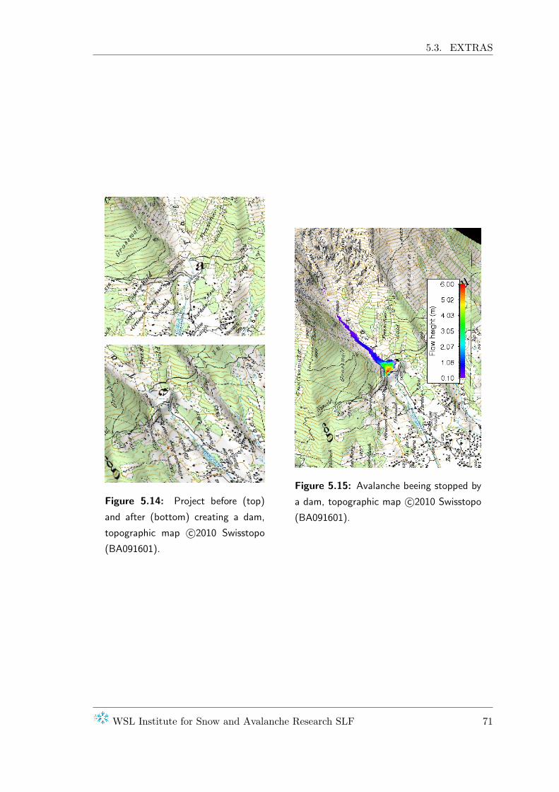
5.3.2 Creating a dam

RAMMS offers the possibility, to simulate a dam by increasing the altitude at the position

where a dam should be considered.

Exercise 5.3.a: How to create a new DEM to simulate a dam.

◦ Create a polygon (”release area”) where a dam is supposed to be build.

◦ Create a second, inner polygon, if you wish to have a two-stage dam.

◦ Go on GIS/GRASS→Add DAM to DEM....

◦ You will be asked to ”Open dam file (*.rel)”. Select the shapefile you want to

use as the outer edge of the dam.

◦ The question pops up, if you want to ”Open 2nd dam shapefile (inner poly-

gon)?”

• Click No to continue with the next step.

• Click Yes to choose 2nd dam file (*.rel).

◦ Next step is to ”Enter TOTAL elevation height of dam (m)”. This is the

elevation (masl.) of the dam crest.

◦ If you loaded an inner polygon file, you will be asked to ”Enter intermediate

height (m)” as well.

◦ At last you have to ”Enter new DEM name”. Your new DEM, containing the

”dam” is created in the folder set as DEM directory (RAMMS preferences ).


To run a simulation based on the new created DEM, you first have to create a new project.

Do almost exactly the same as if creating a regular project without the dam information.

The only important difference is, that you have to choose the correct DEM-file manually

during step 2 of the project wizard.


5.3. EXTRAS

Figure 5.14: Project before (top)

and after (bottom) creating a dam,

topographic map c©2010 Swisstopo

(BA091601).

Figure 5.15: Avalanche beeing stopped by

a dam, topographic map c©2010 Swisstopo

(BA091601).



5.3.3 Creating a new DEM with avalanche deposition

In case you wish to simulate an avalanche flowing down over an old avalanche, you should

take into acount the deposition of the first avalanche, because the path of the second

avalanche will be influenced by the changed terrain.

In output mode RAMMS provides the option of adding the snow height of an avalanche, at

an arbitrary dump step, to the DEM. A new project can be created based on the updated

DEM.

Exercise 5.3.b: How to add avalanche deposition to new DEM.

◦ The deposition height of the avalanche varies with time. So first run the simu-

lation to the specific dump step.

◦ Go to Results→DEM Adaptations→Add Deposition to DEM.

◦ Enter a new name for the new DEM.

◦ The new DEM, containing the deposition information, is created. To run a

simulation based on this DEM create a new project and manually choose the

DEM file during step 2 of the wizard as explained above for the dam.



5.4. HOW TO SAVE INPUT FILES AND PROGRAM SETTINGS

5.4 How to save input files and program settings

Once a project is created, it is saved under the name and location you entered during

step 1 of the RAMMS::Avalanche Project Wizard (see figure 4.5 on page 29). The created

inputfile has the ending *.av2.

The second situation in which the input file is saved automatically, is when a calculation

is started. The saved input file has the same name as the created output file.

Exercise 5.4.a: How to save input files and program settings

manually.

a) Input file:

◦ In case you want to save the input file manually before running a calculation,

go on Track→Save. This is helpful, when a release area and muxi-file was

loaded but you wish to close the project before doing the calculation.

◦ If you wish to save a copy of your file under a new name, go on Track→Save

Copy As or click .

◦ A window pops up to choose an old file which should be overwritten or to type

in a new name, then click Save.

◦ Continue working on the original file, not the just saved one!

b) Program settings:

◦ If you have moved and/or rotated your project for a better view, you can save

this position by going on Extras→Save Active Position.

◦ You can now get back to this position anytime by choosing Extras→Reload

Position.




5.5 How to open input and output files

Exercise 5.5.a: How to open an input file.

◦ Close any active project file.

◦ Go to Track→Open...→Inputfile or click .

◦ A window opens to browse for an avalanche input file (*.av2).

◦ Click Open after file name was selected.

◦ The project will be opened.


Exercise 5.5.b: How to open an output file/avalanche simulation.

◦ Close any active project file.

◦ Go to Track→Open...→Avalanche Simulation or click .

◦ A window opens to browse for an avalanche simulation file (*.out.gz)

◦ Click OK.

◦ The simulation will be opened.

End of Example 5.5.b

Exercise 5.5.c: How to load an optional shapefile.

◦ To load a shapefile, click .

◦ A window opens to browse for a shapefile (*.shp).

◦ Click Open after file was selected.

End of Example 5.5.c


5.6. ABOUT RAMMS

5.6 About RAMMS

Some information about the RAMMS installation on your computer is found here: ?→About

RAMMS....

Figure 5.16: About RAMMS...


6 Program Overview

RAMMS is a windows-based program that relies on drop-down menus and dialogue boxes

to set the model parameters, run calculations and view results. Toolbar buttons are also

available and provide short-cuts of the menu paths; moving the cursor over a button results

in a short explanation, appearing in a text box below the cursor (’tooltip’). For functions

not available in the current context, the menus and buttons are deactivated and cannot

be used.

77

CHAPTER 6. PROGRAM OVERVIEW

Figure 6.1: Graphical user interface (GUI).

6.1 The Graphical User Interface (GUI)

The graphical user interface (GUI), see figure 6.1 on page 78, consists of menu bar, horizon-

tal and vertical toolbar, main window, time step slider, right and left status bar, colorbar

and panel. They will be explained in the following sections.

6.1.1 The menu bar

Track

Similar to the Microsoft Windows ’File’ menu, ’Track’ is used to open, close, save, print,

backup and export files.

New... I Project Wizard

Start a new project, guided by the avalanche wizard (Ctrl+w).

New... I Convert XYZ − > ASCII Grid

Convert laser scanning data into a ESRI ASCII grid.

Open... I Input File


6.1. THE GRAPHICAL USER INTERFACE (GUI)

Open an existing input file (*.av2) (Ctrl+O).

Open... I Avalanche Simulation

Open existing avalanche simulation (select the folder containing the simulation files)

(Ctrl+A).

Close

Close active file (input or output).

Save

Save active file (Ctrl+S)

Save Copy As

Save a copy of the active file (e.g. test.av2 ) under a new name (e.g. simulation1.av2,

works only in input mode). But, RAMMS stays with the active file (test.av2 )!

Export... I Export Display To Image File Create a Image of the active window in

a chosen formate. You can chose the desired image format using the file extension (e.g.

.png, .jpg, .gif, .tif etc.)

Export... I Export GIF Animation Create a GIF Animation of the simulation (only

in OUTPUT mode). Change GIF Animation Interval (s) in the Avalanche tab of the

preferences.

Export... I Export Display To EPS Create an EPS-file of the active window.

Backup... I Backup RAMMS Version Make a backup of the current RAMMS

version.

Backup... I Backup Active Project Backup your active project. The user will be

asked if he wants to include output files in the backup. This function is useful when

having problems with a simulation. Make a backup and send the zip-file together with

some explanations to [email protected]. Make sure that all your input data (release area

shapefiles, MuXi files, domain files, etc...) is in the project folder.

Backup... I Backup User-Defined Files/Folders Backup any folder or files you

want.

Preferences Change RAMMS preferences.

Log files... I RAMMS Logfile (current) Show active RAMMS logfile.

Log files... I RAMMS Logfile (last session) If RAMMS crashed, open this logfile



and copy/paste the content into an email to [email protected].

Install CYGWIN/GRASS Install CYGWIN and GRASS.

Exit Exit RAMMS (Ctrl+Q).

Edit

This menu is used to edit colorbar and dataspace properties. It is active only in input

mode.

Edit Colorbar Properties Edit the colorbar properties.

Edit Dataspace Properties Edit your dataspace properties.

Input

Menu used to specify the global parameters, the calculation domain, release area, friction

parameters and forest cover. This menu is active only in input mode.



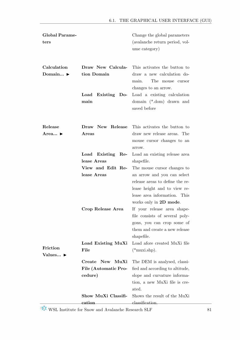
Global Parame-

ters

Change the global parameters

(avalanche return period, vol-

ume category)

Calculation

Domain... I

Draw New Calcula-

tion Domain

This activates the button to

draw a new calculation do-

main. The mouse cursor

changes to an arrow.

Load Existing Do-

main

Load a existing calculation

domain (*.dom) drawn and

saved before

Release

Area... I

Draw New Release

Areas

This activates the button to

draw new release areas. The

mouse cursor changes to an

arrow.

Load Existing Re-

lease Areas

Load an existing release area

shapefile.

View and Edit Re-

lease Areas

The mouse cursor changes to

an arrow and you can select

release areas to define the re-

lease height and to view re-

lease area information. This

works only in 2D mode.

Crop Release Area If your release area shape-

file consists of several poly-

gons, you can crop some of

them and create a new release

shapefile.

Friction

Values... I

Load Existing MuXi

File

Load afore created MuXi file

(*muxi.shp).

Create New MuXi

File (Automatic Pro-

cedure)

The DEM is analysed, classi-

fied and according to altitude,

slope and curvature informa-

tion, a new MuXi file is cre-

ated.

Show MuXi Classifi-

cation

Shows the result of the MuXi

classification.



Forest... I Draw New Forest

Area

The mouse cursor changes to

an arrow and you can draw

new forest areas. Save the for-

est shapefile and then use the

function below (Import Forest

Area From SHAPEFILE) to

import the forest cover.

Show Active Forest

Cover

If forest cover is taken into

account, the corresponding

shapefile is displayed. If your

project uses no forest cover at

the moment, RAMMS will tell

you so.

Import Forest Area

From SHAPEFILE

If a forest shapefile has been

drawn (using ) it can be im-

ported using this function.

Import Forest Area

From ASCII Grid

If a forest ASCII grid is avail-

able, it can be imported using

this function (0=no forest, 1

= forest).

Remove Active For-

est Cover

Remove the active forest

raster data from the project.



Show

This menu enables and disables the different visualizations. A little arrow indicates if the

visualization is enabled or disabled.

Show Lights Show/hide light effects

Show Grid Show/hide computational grid

Show Map Show map

Show Image Show orthophoto/image

Show Release Area/Simulation Show/hide release area (input mode) or

simulation results (output mode)

Show Isotropic View Switch between realistic (isotropic) and

anisotropic view

Show Colorbar Show/hide colorbar

Show Bottom Color Show/hide 0-color

Show Arrow OUTPUT — Show/hide point arrow of

time plot

Show Line Profile OUTPUT — Show/hide line of line

profile

Show Domain Show/hide calculation domain area

(only in input mode)



Run

This menu is active only in input mode.

Run Avalanche Simulation Opens the module parameter window

to change parameters and to start the

calculation

Results

This menu contains the results functions and is only active in output mode.



Flow Height Shows flow height of the

avalanche for every time step.

Flow VelocityShows flow velocity of the


Flow PressureShows flow pressure of the


Flow Momen-

tum

Shows flow momentum of the


Max

Values... I

Max Flow Height Displays the maximum flow

height for each cell.

Max Velocity Displays the maximum veloc-

ity for each cell.

Max Pressure Displays the maximum pres-

sure for each cell.

Max Momentum Displays the maximum mo-

mentum for each cell.

DEM

Adaptations I

Add Deposition to

DEM

Adds the deposition of an

avalanche simulation to a new

DEM.

Flow

Analysis... I

Summary of Moving

Mass

Summarizes the Moving

Mass.

Friction

Parameters I

Mu Display mu for this simula-

tion.

Xi Display xi for this simulation.



GIS/GRASS

This menu contains GIS and GRASS functions.

Import Polygon Shapefile Import a ESRI GIS polygon shapefile.

Convert Shapefile... Converts a normal polygon shape-

file into a RAMMS release file or a

RAMMS forest file. This function

makes only sense in the input mode.

Export Results As Shapefile Export the active results to an ESRI

GIS shapefile for later use in a GIS pro-

gram.

Export Results As ASCII Grid Export the active results to an ESRI

ASCII Grid for later use in a GIS pro-

gram.

Add Dam to DEM... Adds a Dam to the DEM. You have to

specify relative Dam height or absolute

Dam elevation.

Show Slope Angle (◦) Display the slope angles.

Show Curvature (1/m) Display the curvatures.

Show Contour Plot Display a contour plot.

Resample Slope/Curvature Normally, slope and curvatures are cal-

culated for a grid resolution of 10m.

You can change this resolution by using

this function.

GRASS Advanced... These are advanced GRASS functions.

You should only use them if you know

what you are doing.

GRASS Logfiles... Logfiles of all the GRASS functions are

provided here. If your MuXi file looks

strange, have a look at the MuXi Log-

file.



Extras

Add/Change or Remove map Add or change the topographic map

of your project. The maps have to

be located in your distribution’s ’Map’

folder, see section 3.5 for details. If not,

you can browse for the maps.

Add/Change or Remove Imagery Add, change or remove the imagery

used for visualization of your project.

The images have to be located in your

distribution’s ’IMAGE’ folder, see sec-

tion 3.5 for details. If not, you can

browse for the images.

Point... Used to select points in OUTPUT

mode, save point locations and export

Time Plot Data.

Profile... Used to draw a profile in OUTPUT

mode, save profile points and export

Profile Plot Data.

Save Active Position Save your current state of view, as well

as the enabled and disabled visualiza-

tions.

Reload Position Reload your saved position.

Google Earth... This function exports release areas,

muxi files and your results to Google

Earth. See Map Options for map set-

tings for areas outside of Switzerland.

Map Options Dialogue window to enter map settings

(projection, datum, offsets...) for areas

outside of Switzerland.



Project

This menu contains the project input and output logfiles.

Project Input Log

Displays the input logfile.

Project Output Log

Displays the output logfile. The input logfile is appended to the output logfile.

Help

Manuals... I User Manual (PDF) RAMMS User Manual

Friction Parameter

Table (PDF)

RAMMS friction parameter

table

RAMMS web... RAMMS Homepage at

http://ramms.slf.ch

Updates... Download RAMMS updates

manually or directly from the

web

About

RAMMS...

About dialog window

License Agree-

ment...

RAMMS License Agreement

Release Notes Information about the

RAMMS release


http://ramms.slf.ch


6.1.2 Horizontal toolbar

Project wizard: open avalanche wizard for creating a new

avalanche project.

Open input file.

Open simulation.

Save copy as: save the active file under a new name (input).

Close: close the active file (input and output).

Print: displays the Windows print manager.

Undo, Redo.

Arrow (move and resize), Rotate, Move.

Simulation Results: Choose this function and move the arrow over

the topography → x-, y- and z-Coordinates of the mouse position

are shown in the lower right status bar (see below).

OUTPUT | If you move the arrow over the simulation data, the

active parameter is shown as well (see right value in the figure

below). If you click once with the left mouse button at a point of

interest, a new window pops up called ’RAMMS::Avalanche Time

Plot <Active Parameter>’.

INPUT, 2D | Crop Release Areas: Click this button to make a

selection of the release area polygons you want to crop.

INPUT, 2D | View and Edit Release Areas.

INPUT, 2D | Create new release area: specify new polygon-points

by clicking with left mouse button, for the last polygon-point use

a double-click to finish. The user is asked if he wants to draw

more release areas. At last, he has to specify a new filename for

the release area.

INPUT, 2D | Create new forest area: specify new polygon-points

by clicking with left mouse button, for the last polygon-point use

a double-click to finish. The user is asked if he wants to draw

more forest areas. At last, he has to specify a new filename for

the forest area.



INPUT, 2D | Create new domain area: specify a new domain

polygon by clicking with left mouse button, for the last polygon-

point use a double-click to finish. A dialogue box will then ask the

user for a new domain name (e.g. test).

OUTPUT, 2D | Line Profile: Select the topography, until the

Line-Profile-Button is active. Click the button and then move

the cursor to the start point of your profile. Click the left mouse

button and move the cursor to the next position of your profile.

At the end position of your profile double click with the left mouse

button. A new window pops up called ’RAMMS::Avalanche Line

Profile Plot Active Parameter’. This line profile plot is linked to

your simulation. If you change the parameter or if you change the

max-value in the avalanche-panel, the changes are adapted in the

line profile plot!

Zoom tools.

Annotation tools: text, line, rectangle, oval, polygon, freehand.



6.1.3 Vertical toolbar

Add shapefile (*.shp).

Show/hide lights.

Show/hide mesh.

Show map.

Show image.

INPUT | Show/hide release area (or other active parameter).

OUTPUT | Show/hide simulation.

Switch between isotropic and anisotropic view.

Show/hide colorbar.

INPUT | Run Simulation.

OUTPUT | Animate Simulation / Continue Simulation.

Stop/Pause Simulation ( ).

OUTPUT | End Simulation: skip to last dump step of simulation.

Create a screenshot of the main window.

OUTPUT | Create GIF animation.

Edit colorbar properties.

Edit dataspace properties.

Change RAMMS preferences (e.g. working directory).

Change view to 2D / Change view to 3D ( ).

6.1.4 Main window

All input and output related visualizations are displayed in the main window.

6.1.5 Time step slider (only OUTPUT)

The time step slider can be moved manually to change the active time step.



6.1.6 Left status bar

The left status bar is used to display status information for operations or informational

messages pertaining to the currently selected surface or manipulators.

6.1.7 Right status bar

The right status bar is used to display the position of the cursor within the surface and

additionally simulation results at the position of the cursor.

Figure 6.2: Position information and triangle simulation results in the right status bar.

6.1.8 Colorbar

In general, the colorbar appears at the

right edge of the main window (see figure

6.1) and can be moved and resized (see ex-

ercise ”Editing the colorbar” on page 49).Figure 6.3: Colorbar

6.1.9 Panel

An avalanche panel is displayed on the right side of the RAMMS GUI (see fig. 6.4),

and consists of four tabs (General, Display, Volumes and Region). This panel changes

interactively, depending on what parameter is displayed in the main window. The current

parameter (A-1)and all visualizations (A-2) are additional information/functions on the

avalanche panel.

General Tab

The General tab (A) shows some important simulation parameters, such as: nr. of nodes,

nr. of cells, end time (s), dump step (s), grid resolution (m) and avalanche density (kg/m3).



Figure 6.4: Avalanche panel.

Display Tab

The Display tab (B) shows parameters that are important for the display (colors, trans-

parency) of results and polygon shapefiles. The Min and Max values as well as the number

of colors influence directly the colorbar and the visualization. The transparency of the sim-

ulation results can be changed on the avalanche-display-panel. 0% means no transparency,

100% means total transparency, see figure below (fig. 6.5). The colorbar is devided into

n (nr. of colors) different colors, where the lowest color is normally not displayed. The

bottom line informs the user of the range of the values that are not displayed in the current

visualization (only in output mode).

Volumes Tab

The Volumes tab (C) gives the user information about the release area, such as projected

release area, 3D release area, estimated release volume (input mode), release mass (input)



Figure 6.5: No transparency (left) and 40% transparency (right) of simulation result.

and calculated release volume (output). The input release volume is estimated. Normally,

the calculated release area is 1%− 7% larger than the estimated values.

Region Tab

The Region Tab (D) gives information about min and max X-, Y-coordinates and the

altitude limits as well as an information about the region area in km2.


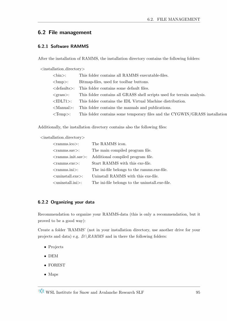
6.2. FILE MANAGEMENT

6.2 File management

6.2.1 Software RAMMS

After the installation of RAMMS, the installation directory contains the following folders:

<installation directory>

<bin>: This folder contains all RAMMS executable-files.

<bmp>: Bitmap-files, used for toolbar buttons.

<defaults>: This folder contains some default files.

<grass>: This folder contains all GRASS shell scripts used for terrain analysis.

<IDL71>: This folder contains the IDL Virtual Machine distribution.

<Manual>: This folder contains the manuals and publications.

<Temp>: This folder contains some temporary files and the CYGWIN/GRASS installation file.

Additionally, the installation directory contains also the following files:

<installation directory>

<ramms.ico>: The RAMMS icon.

<ramms.sav>: The main compiled program file.

<ramms init.sav>: Additional compiled program file.

<ramms.exe>: Start RAMMS with this exe-file.

<ramms.ini>: The ini-file belongs to the ramms.exe-file.

<uninstall.exe>: Uninstall RAMMS with this exe-file.

<uninstall.ini>: The ini-file belongs to the uninstall.exe-file.

6.2.2 Organizing your data

Recommendation to organize your RAMMS-data (this is only a recommendation, but it

proved to be a good way):

Create a folder ’RAMMS’ (not in your installation directory, use another drive for your

projects and data) e.g. D:\RAMMS and in there the following folders:

• Projects

• DEM

• FOREST

• Maps



• OrthoPhoto

It is important, that the DEM and forest files, as well as your georeferenced maps and

imagery, are located in the appropriate folders. These folders are the ones selected in the

RAMMS preferences (how to set the correct folders see section 3.5).

IMPORTANT: There should be no blanks or special characters in all the above directories.

For example, do not specify a working directory like C:\Documents and Settings\Eigene

Dateien\Data etc...this will not work for RAMMS.


List of Figures

3.1 Installation - Welcome dialog window. . . . . . . . . . . . . . . . . . . . . . 6

3.2 Installation - Readme dialog window. . . . . . . . . . . . . . . . . . . . . . . 6

3.3 Installation - License agreement dialog window. . . . . . . . . . . . . . . . . 7

3.4 Installation - Destination directory dialog window. . . . . . . . . . . . . . . 7

3.5 Installation - Installing files dialog window. . . . . . . . . . . . . . . . . . . 8

3.6 Installation - Finished installing files dialog window. . . . . . . . . . . . . . 8

3.7 Installation - Finished installation dialog window. . . . . . . . . . . . . . . . 9

3.8 RAMMS icon. . . . . . . . . . . . . . . . . . . . . . . . . . . . . . . . . . . . 9

3.9 RAMMS program group. . . . . . . . . . . . . . . . . . . . . . . . . . . . . 9

3.10 RAMMS start window. . . . . . . . . . . . . . . . . . . . . . . . . . . . . . 11

3.11 RAMMS licensing window. . . . . . . . . . . . . . . . . . . . . . . . . . . . 11

3.12 Enter user name and company name. . . . . . . . . . . . . . . . . . . . . . . 12

3.13 Personal license request file RAMMS request Muster Test.txt . . . . . . . . 12

3.14 Personal license key file RAMMS license Muster Test.txt . . . . . . . . . . . 13

3.15 Continue Cygwin/GRASS installation? . . . . . . . . . . . . . . . . . . . . . 13

3.16 Choose Cygwin/GRASS installation zip-file. . . . . . . . . . . . . . . . . . . 14

3.17 Choose Cygwin/GRASS installation directory. . . . . . . . . . . . . . . . . 15

3.18 Cygwin/GRASS - Extract files. . . . . . . . . . . . . . . . . . . . . . . . . . 16

3.19 Cygwin/GRASS - Add to registry. . . . . . . . . . . . . . . . . . . . . . . . 16

3.20 Cygwin/GRASS - Registered successfully. . . . . . . . . . . . . . . . . . . . 16

3.21 Cygwin/GRASS - Automatic scripts. . . . . . . . . . . . . . . . . . . . . . . 17

3.22 Error message . . . . . . . . . . . . . . . . . . . . . . . . . . . . . . . . . . . 17

3.23 IDL Visual Studio Merge Modules - Welcome dialog window. . . . . . . . . 18

3.24 IDL Visual Studio Merge Modules - Ready to install the Program. . . . . . 18

3.25 IDL Visual Studio Merge Modules - Installing... . . . . . . . . . . . . . . . . 19

3.26 Installation - Destination directory dialog window. . . . . . . . . . . . . . . 19

3.27 General tab of RAMMS preferences. . . . . . . . . . . . . . . . . . . . . . . 21

3.28 Avalanche tab of RAMMS preferences. . . . . . . . . . . . . . . . . . . . . . 21

3.29 RAMMS preferences. . . . . . . . . . . . . . . . . . . . . . . . . . . . . . . . 22

3.30 Browse for the correct folder. . . . . . . . . . . . . . . . . . . . . . . . . . . 22

i

List of Figures

4.1 Project extent (area of interest) - topographic map c©2010 Swisstopo (BA091601). 24

4.2 Example ESRI ASCII Grid. . . . . . . . . . . . . . . . . . . . . . . . . . . . 25

4.3 Example ASCII X,Y,Z single space data. . . . . . . . . . . . . . . . . . . . . 26

4.4 RAMMS Avalanche Project Wizard: Step 1 of 4. . . . . . . . . . . . . . . . 28

4.5 Step 1 of the RAMMS project wizard: Project information. . . . . . . . . . 29

4.6 Window to browse for a new project location. . . . . . . . . . . . . . . . . . 29

4.7 Step 2 of the RAMMS project wizard: GIS information. . . . . . . . . . . . 29

4.8 Project coordinates: lower left and upper right corner of project area -c©2010 swisstopo (BA091601). . . . . . . . . . . . . . . . . . . . . . . . . . 30

4.9 Step 3 of the RAMMS project wizard: Project boundary coordinates. . . . 30

4.10 Step 4 of the RAMMS project wizard: Project summary. . . . . . . . . . . 31

4.11 Created project files. . . . . . . . . . . . . . . . . . . . . . . . . . . . . . . . 34

4.12 ”Active” project with lines and corners for resizing, topographic map c©2010

Swisstopo (BA091601) . . . . . . . . . . . . . . . . . . . . . . . . . . . . . . 36

4.13 ”Active” project with rotation axes, topographic map c©2010 swisstopo

(BA091601). . . . . . . . . . . . . . . . . . . . . . . . . . . . . . . . . . . . . 37

4.14 3D view of example model, topographic map c©2010 swisstopo (BA091601). 38

4.15 2D view of example model, topographic map c©2010 swisstopo (BA091601). 38

4.16 RAMMS global parameters. . . . . . . . . . . . . . . . . . . . . . . . . . . . 39

4.17 Project with emerging release area. . . . . . . . . . . . . . . . . . . . . . . . 41

4.18 Release area and volume information. . . . . . . . . . . . . . . . . . . . . . 43

4.19 Release area information window. . . . . . . . . . . . . . . . . . . . . . . . . 44

4.20 Calculation domain in green confines the area of interest and saves calcula-

tion time. . . . . . . . . . . . . . . . . . . . . . . . . . . . . . . . . . . . . . 45

4.21 RAMMS Voellmy-fluid friction model. . . . . . . . . . . . . . . . . . . . . . 46

4.22 RAMMS — Automatic MuXi Procedure. . . . . . . . . . . . . . . . . . . . 47

4.23 The avalanche ’Display’ panel. . . . . . . . . . . . . . . . . . . . . . . . . . 49

4.24 The colorbar properties window. . . . . . . . . . . . . . . . . . . . . . . . . 50

4.25 RAMMS Project Input Log Information. . . . . . . . . . . . . . . . . . . . . 53

4.26 Region extent (X-, Y- and Z-Coordinates, total area). . . . . . . . . . . . . 54

4.27 Window to choose map image. . . . . . . . . . . . . . . . . . . . . . . . . . 55

5.1 General information. . . . . . . . . . . . . . . . . . . . . . . . . . . . . . . . 58

5.2 Calculation parameters . . . . . . . . . . . . . . . . . . . . . . . . . . . . . . 59

5.3 Friction values MuXi. . . . . . . . . . . . . . . . . . . . . . . . . . . . . . . 59

5.4 Release information. . . . . . . . . . . . . . . . . . . . . . . . . . . . . . . . 59

5.5 Stop criteria. . . . . . . . . . . . . . . . . . . . . . . . . . . . . . . . . . . . 60

5.6 Status window of calculation. . . . . . . . . . . . . . . . . . . . . . . . . . . 61

ii RAMMS User Manual

List of Figures

5.7 Main window in output mode, topographic map c©2010 Swisstopo (BA091601). 61

5.8 MuXi settings for a variable calculation. . . . . . . . . . . . . . . . . . . . . 62

5.9 Results: Maximum values of flow height (left), velocity (middle) and pres-

sure (right), topographic map c©2010 Swisstopo (BA091601). . . . . . . . . 64

5.10 Line profile plot. . . . . . . . . . . . . . . . . . . . . . . . . . . . . . . . . . 65

5.11 Line profile perpendicular to flow direction, topographic map c©2010 Swis-

stopo (BA091601). . . . . . . . . . . . . . . . . . . . . . . . . . . . . . . . . 66

5.12 Line profile along the avalanche path, topographic map c©2010 Swisstopo

(BA091601). . . . . . . . . . . . . . . . . . . . . . . . . . . . . . . . . . . . . 66

5.13 Time plot window. . . . . . . . . . . . . . . . . . . . . . . . . . . . . . . . . 67

5.14 Project before (top) and after (bottom) creating a dam, topographic mapc©2010 Swisstopo (BA091601). . . . . . . . . . . . . . . . . . . . . . . . . . 71

5.15 Avalanche beeing stopped by a dam, topographic map c©2010 Swisstopo

(BA091601). . . . . . . . . . . . . . . . . . . . . . . . . . . . . . . . . . . . . 71

5.16 About RAMMS... . . . . . . . . . . . . . . . . . . . . . . . . . . . . . . . . . 75

6.1 Graphical user interface (GUI). . . . . . . . . . . . . . . . . . . . . . . . . . 78

6.2 Position information and triangle simulation results in the right status bar. 92

6.3 Colorbar . . . . . . . . . . . . . . . . . . . . . . . . . . . . . . . . . . . . . . 92

6.4 Avalanche panel. . . . . . . . . . . . . . . . . . . . . . . . . . . . . . . . . . 93

6.5 No transparency (left) and 40% transparency (right) of simulation result. . 94

WSL Institute for Snow and Avalanche Research SLF iii

List of Exercises

3.5.a: Working directory . . . . . . . . . . . . . . . . . . . . . . . . . . . . . . . . 22

4.3.a: How to create a new project. . . . . . . . . . . . . . . . . . . . . . . . . . . 28

4.4.a: Moving and resizing the model . . . . . . . . . . . . . . . . . . . . . . . . . 36

4.4.b: Rotating the model . . . . . . . . . . . . . . . . . . . . . . . . . . . . . . . 37

4.4.c: How to switch between 2D and 3D mode . . . . . . . . . . . . . . . . . . . 38

4.6.a: How to create a new release area. . . . . . . . . . . . . . . . . . . . . . . . 41

4.6.b: How to load an existing release area. . . . . . . . . . . . . . . . . . . . . . 42

4.6.c: Specify release height and view release information . . . . . . . . . . . . . 44

4.8.a: How to create a new MuXi file. . . . . . . . . . . . . . . . . . . . . . . . . 48

4.8.b: How to load an existing MuXi file. . . . . . . . . . . . . . . . . . . . . . . 48

4.9.a: Editing the colorbar . . . . . . . . . . . . . . . . . . . . . . . . . . . . . . . 49

4.10.a: How to create a new FOREST file. . . . . . . . . . . . . . . . . . . . . . . 52

4.12.a: How to add or change maps. . . . . . . . . . . . . . . . . . . . . . . . . . 55

4.12.b: How to add or change remote sensing imagery. . . . . . . . . . . . . . . . 56

5.1.a: How to run a constant avalanche calculation. . . . . . . . . . . . . . . . . . 58

5.1.b: How to run a variable MuXi avalanche calculation. . . . . . . . . . . . . . 62

5.2.a: Displaying max values. . . . . . . . . . . . . . . . . . . . . . . . . . . . . . 64

5.2.b: How to draw a line profile. . . . . . . . . . . . . . . . . . . . . . . . . . . . 65

5.2.c: How to create a time plot. . . . . . . . . . . . . . . . . . . . . . . . . . . . 67

5.2.d: Enter point coordinates and get a time plot. . . . . . . . . . . . . . . . . . 68

5.3.a: How to create a new DEM to simulate a dam. . . . . . . . . . . . . . . . . 70

5.3.b: How to add avalanche deposition to a new DEM. . . . . . . . . . . . . . . 72

v

List of Exercises

5.4.a: How to save input files and program settings manually. . . . . . . . . . . . 73

5.5.a: How to open an input file. . . . . . . . . . . . . . . . . . . . . . . . . . . . 74

5.5.b: How to open an output file/avalanche simulation. . . . . . . . . . . . . . . 74

5.5.c: How to load an optional shapefile. . . . . . . . . . . . . . . . . . . . . . . . 74

vi RAMMS User Manual

Index

A

Add Dam to DEM, 86

Add/Change Image, 87

Add/Change Map, 87

Avalanche wizard, 28

B

Backup Active Project, 79

Backup RAMMS Version, 79

Backup User-Defined Files/Folders, 79

C

Calculation Domain, 45

Colorbar, 92

Edit, 49

Convert Shapefile..., 86

Create New MuXi File (Automatic Pro-

cedure), 81

Crop Release Areas, 81

D

Dam, 70, 72

DEM

Create new, 70, 72

Draw New Calculation Domain, 81

Draw New Forest Area, 82

Draw New Release Area, 81

dump step slider, 91

E

Edit Colorbar Properties, 80

Edit Dataspace Properties, 80

Exit, 80

Export Display To EPS, 79

Export Display To Image File, 79

Export GIF Animation, 79

Export Result To Google Earth, 87

Export Results As ASCII Grid, 86

Export Results As Shapefile, 86

F

File management, 95

Files

*.tfw, 55

world, 55

Flow Height, 85

Flow height, 63

Max flow height, 63

Flow Momentum, 85

Flow momentum, 63

Max momentum, 63

Flow Pressure, 85

Flow pressure, 63

Max pressure, 63

Flow Velocity, 85

Flow velocity, 63

Max velocity, 63

Forest, 51

Create FOREST-file, 51

Influence on friction parameters, 51

Forest information, 25

Friction parameter, 46

Create new MuXi file, 47

vii

List of Exercises

Load MuXi file, 47

Mu, 46

Xi, 46

Friction Parameters..., 85

G

Global Parameters, 81

Global parameters, 26, 39

Graphical User Interface, 78

Colorbar, 78

Main window, 78

Menu bar, 78

Edit, 80

Extras, 87

GIS/GRASS, 86

Help, 88

Input, 80

Project, 88

Results, 84

Run, 84

Show, 83

Track, 78

Panel, 78

Status bar, 78

Time step slider, 78

Toolbar buttons, 78

GRASS Advanced..., 86

GRASS Logfiles..., 86

I

Import Forest Area From ASCII Grid, 82

Import Forest Area From SHAPEFILE,

82

Import GIS Polygon Shapefile, 86

Install CYGWIN/GRASS, 80

Installation, 5

L

Licensing Methods, 10

Load

MuXi file, 47

Release file, 40

Load Existing Domain, 81

Load Existing MuXi File, 81

Load Existing Release Area, 81

M

Main window, 91

Map

Add, 55

Change, 55

Load new, 55

Map Options, 87

Max Flow Height, 85

Max Momentum, 85

Max Pressure, 85

Max Velocity, 85

Move, 36

O

Open

Input file, 74

Output file, 74

Shapefile, 74

Orthophoto

Add, 55

Change, 55

Load new, 56

P

Panel

Avalanche Panel, 92

Display, 92

General, 92

Region, 92

Transparency, 93

Volumes, 92

Point..., 87

viii RAMMS User Manual

Index

Preferences, 20, 22, 79

Set DEM directory, 20

Set FOREST directory, 20

Set Map directory, 20

Set Orthophoto directory, 20

Set Working directory, 20, 22

Profile..., 87

Project

Create new, 28

General, 23

Information, 53

Input data, 24

Model input data, 24

Scenarios, 23

Wizard, 27

R

RAMMS Logfile (current), 79

RAMMS Logfile (last session), 79

Release area, 40

Create manually, 40

Load, 40

Release information, 44

shapefile, 40

Release information, 26

Reload Position, 87

Remove Active Forest Cover, 82

Resample Slope/Curvature, 86

Resize, 36

Results, 63

Flow height, 63

Flow momentum, 63

Flow pressure, 63

Flow velocity, 63

Line profile, 63, 64

Max values, 63, 64

Time plot, 64

Run calculation

Calculation Domain, 45

Constant, 57

Variable, 63

S

Save

automatically, 73

manually, 73

Save Active Position, 87

Shapefile

Load, 74

Show Active Forest Cover, 82

Show Contour Plot, 86

Show Curvature, 86

Show MuXi Classification, 81

Show Slope Angle, 86

Status bar

Left, 92

Right, 92

System Requirements, 5

T

TFW-files, 55

Toolbar

Horizontal, 89

Vertical, 91

Transparency, 93

V

View and Edit Release Area, 81

W

world-files, 55

WSL Institute for Snow and Avalanche Research SLF ix