STA347 - week 3 1

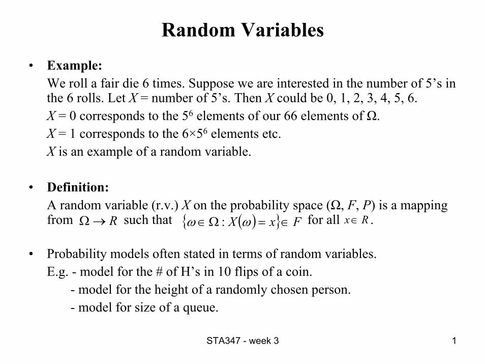
Random Variables• Example:

We roll a fair die 6 times. Suppose we are interested in the number of 5’s in the 6 rolls. Let X = number of 5’s. Then X could be 0, 1, 2, 3, 4, 5, 6. X = 0 corresponds to the 56 elements of our 66 elements of Ω.X = 1 corresponds to the 6×56 elements etc.X is an example of a random variable.

• Definition:A random variable (r.v.) X on the probability space (Ω, F, P) is a mapping from such that for all .

• Probability models often stated in terms of random variables.E.g. - model for the # of H’s in 10 flips of a coin.

- model for the height of a randomly chosen person.- model for size of a queue.

R→Ω ( ) FxX ∈=Ω∈ ωω : Rx∈

STA347 - week 3 2

Discrete Probability Spaces (Ω, F, P)

STA347 - week 3 3

Discrete Random Variable• Definition:

A random variable X is said to be discrete if it can take only a finite or countablyinfinite number of distinct values.

• A discrete random variable X maps the sample space Ω onto a countable set. Define a probability mass function (pmf) or frequency function on X such that

Where the sum is taken over all possible values of X.• Note that there is a theorem that states that there exists a probability triple and

random variable whenever we have a function p such that

• Definition:The probability distribution of a discrete random variable X is represented by a formula, a table or a graph which provides the list of all possible values that X can take and the pmf for each value

STA347 - week 3 4

Examples of Discrete Random Variables

• Discrete Uniform DistributionWe roll a fair die. Let X = the # that comes up. We have that This is an example of equiprobable outcomes, that is

To state the probability distribution of X we need to give its possible values and its pmf

X is a discrete Uniform random variable. X has a uniform distribution.

( ) ωω =X

STA347 - week 3 5

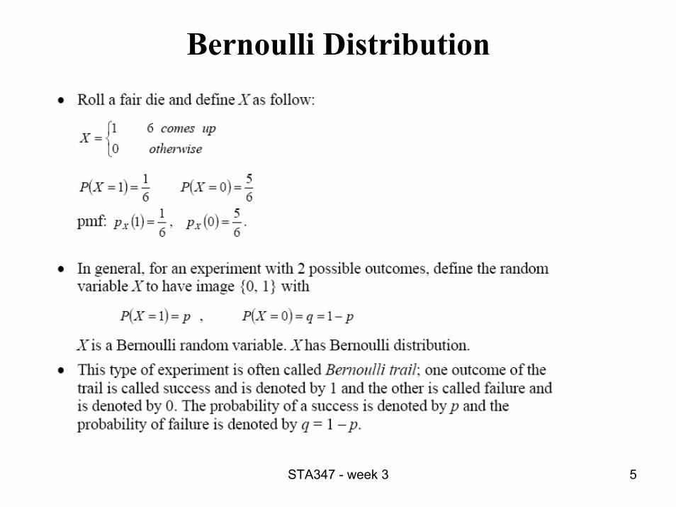
Bernoulli Distribution

STA347 - week 3 6

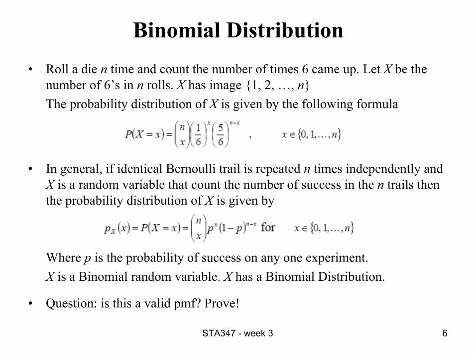
Binomial Distribution• Roll a die n time and count the number of times 6 came up. Let X be the

number of 6’s in n rolls. X has image 1, 2, …, nThe probability distribution of X is given by the following formula

• In general, if identical Bernoulli trail is repeated n times independently and X is a random variable that count the number of success in the n trails then the probability distribution of X is given by

Where p is the probability of success on any one experiment.X is a Binomial random variable. X has a Binomial Distribution.

• Question: is this a valid pmf? Prove!

STA347 - week 3 7

Geometric Distribution

• We roll a fair die until the first 6 comes up. Let X = the number of rolls until we get the first 6.Possible values of X: 1, 2, 3, …..The probability distribution of X is given by the following formula

• In general, if identical Bernoulli trail is repeated independently until the first success is obtained and X is a random variable that count the number of trials until the first success then the probability distribution of X is given by

X is a Geometric random variable. X has a Geometric Distribution.

• Question: is this a valid pmf? Prove!

STA347 - week 3 8

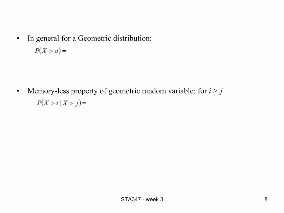
• In general for a Geometric distribution:

• Memory-less property of geometric random variable: for i > j

STA347 - week 3 9

Negative Binomial Distribution• We roll a fair die until the second 6 comes up. This is the waiting time for the

second 6. Let X = the number of rolls until we get two 6’s.Possible values of X: 2, 3, 4, …..The probability distribution of X is given by the following formula

• Is this a valid pmf? Prove!

• In general, X is the total number of experiments when waiting for rth success in a sequence of independent Bernoulli trails. The probability distribution of X is given by

X has a Negative Binomial random Distribution.

STA347 - week 3 10

Hypergeometric Distribution

• A hat contains 12 tickets, 7 black and 5 white. Three tickets are drawn at random. Let X = the # of black tickets drawn. X could be 0, 1, 2, 3.The probability mass for each value can be calculated using combinatorics. For example,

STA347 - week 3 11

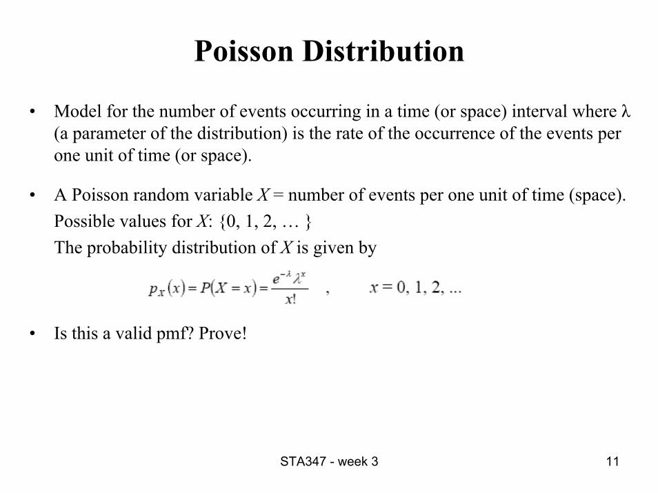
Poisson Distribution

• Model for the number of events occurring in a time (or space) interval where λ(a parameter of the distribution) is the rate of the occurrence of the events per one unit of time (or space).

• A Poisson random variable X = number of events per one unit of time (space). Possible values for X: 0, 1, 2, … The probability distribution of X is given by

• Is this a valid pmf? Prove!

STA347 - week 3 12

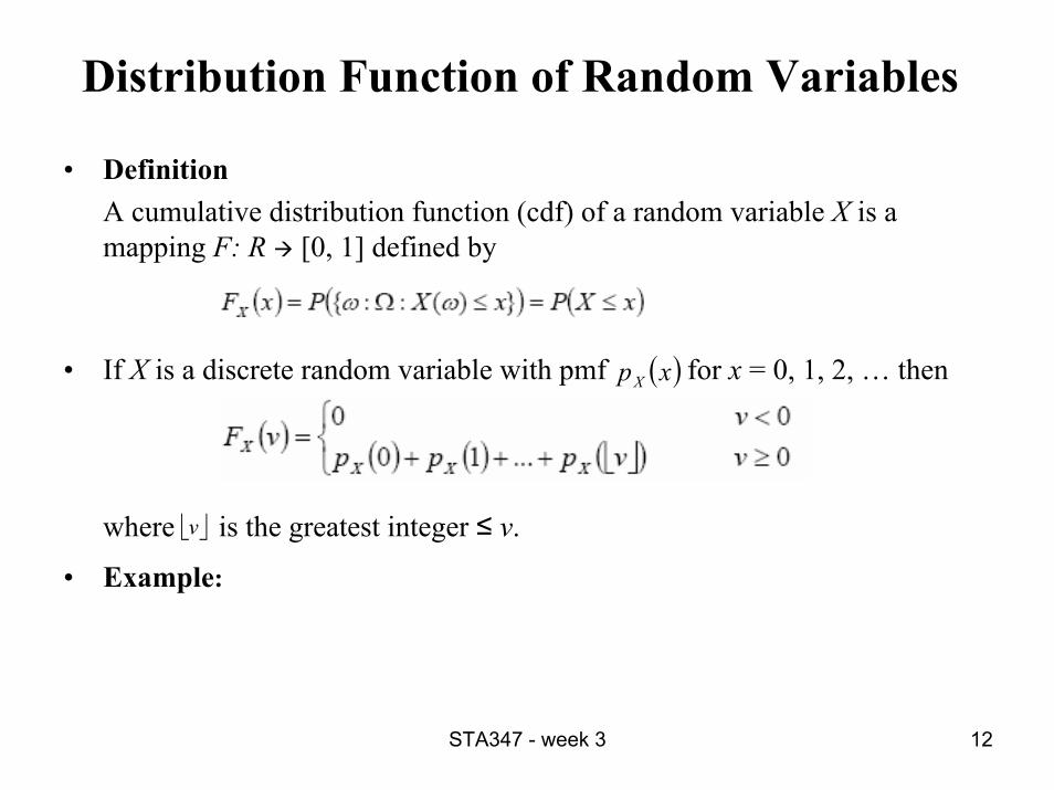
Distribution Function of Random Variables

• DefinitionA cumulative distribution function (cdf) of a random variable X is a mapping F: R [0, 1] defined by

• If X is a discrete random variable with pmf for x = 0, 1, 2, … then

where is the greatest integer ≤ v.

• Example:

⎣ ⎦v

( )xpX

STA347 - week 3 13

Properties of Distribution Function

• F is monotone, non decreasing i.e. F(x) ≤ F(y) if x ≤ y.

• As x - ∞ , F(x) 0

• As x ∞ , F(x) 1

• F(x) is continuous from the right

• For a < bWhy?

( ) ( ) ( )aFbFbXaP XX −=≤<

STA347 - week 3 14

Relation between Binomial and Poisson Distributions

• Binomial distribution

Model for number of success in n trails where P(success in any one trail) = p.

• Poisson distribution is used to model rare occurrences that occur on average at rate λ per time interval. Can think of “rare” occurrence in terms of p 0 and n ∞. Take these limits so that λ = np.

• So we have that

STA347 - week 3 15

Exercises

1. A box contain 20 notes numbered 20 to 39. We randomly pick one note and record its number. What is the probability that the number we got is greater then 32?

2. 30% of U of T students wear glasses. We select a random sample of size 10 students. a) What is the probability that exactly 4 of them wear glasses?b) What is the probability that more then 3 wear glasses?

3. We roll a die until we obtained an even outcome. a) What is the probability that we will roll the die exactly 5 times? b) What is the probability that we roll the die more then 7 times ? c) What is the probability that we roll the die more then 7 times if we

know that we need more then 2 rolls?

STA347 - week 3 16

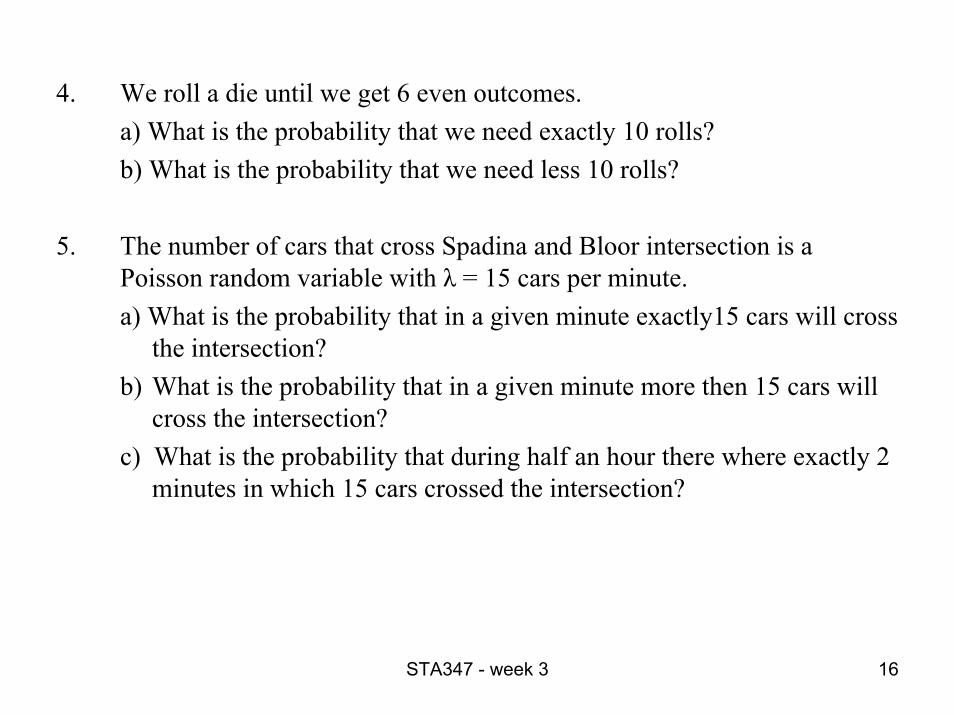
4. We roll a die until we get 6 even outcomes.a) What is the probability that we need exactly 10 rolls?b) What is the probability that we need less 10 rolls?

5. The number of cars that cross Spadina and Bloor intersection is a Poisson random variable with λ = 15 cars per minute.a) What is the probability that in a given minute exactly15 cars will cross

the intersection?b) What is the probability that in a given minute more then 15 cars will

cross the intersection?c) What is the probability that during half an hour there where exactly 2

minutes in which 15 cars crossed the intersection?

STA347 - week 3 17

Continuous Probability Spaces

• Ω is not countable.

• Outcomes can be any real number or part of an interval of R, e.g. heights, weights and lifetimes.

• Can not assign probabilities to each outcome and add them for events.

• Define Ω as an interval that is a subset of R.

• F – the event space elements are formed by taking a (countable) number of intersections, unions and complements of sub-intervals of Ω.

• Example: Ω = [0,1] and F = A = [0,1/2), B = [1/2, 1], Φ, Ω

STA347 - week 3 18

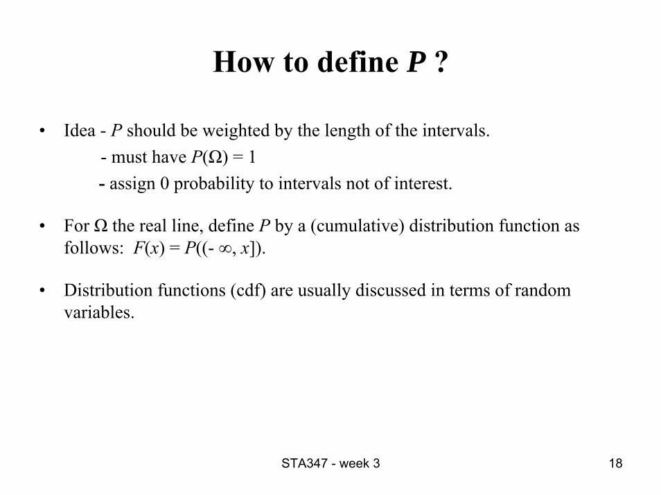
How to define P ?

• Idea - P should be weighted by the length of the intervals.- must have P(Ω) = 1- assign 0 probability to intervals not of interest.

• For Ω the real line, define P by a (cumulative) distribution function as follows: F(x) = P((- ∞, x]).

• Distribution functions (cdf) are usually discussed in terms of random variables.

STA347 - week 3 19

Recalls

STA347 - week 3 20

Cdf for Continuous Probability Space

• For continuous probability space, the probability of any unique outcome is 0. Because,

P(ω) = P((ω, ω]) = F(ω) - F(ω) = 0.

• The intervals (a, b), [a, b), (a, b], [a, b] all have the same probability in continuous probability space.

• Generally speaking, – discrete random variable have cdfs that are step functions.– continuous random variables have continuous cdfs.

STA347 - week 3 21

Examples(a) X is a random variable with a uniform[0,1] distribution.

The probability of any sub-interval of [0,1] is proportional to the interval’s length. The cdf of X is given by:

(b) Uniform[a, b] distribution, b > a. The cdf of X is given by:

STA347 - week 3 22

Formal Definition of continuous random variable

• A random variable X is continuous if its distribution function may be written in the form

for some non-negative function f.

• fX(x) is the (Probability) Density Function of X.

• Examples are in the next few slides….

STA347 - week 3 23

The Uniform distribution

(a) X has a uniform[0,1] distribution. The pdf of X is given by:

(b) Uniform[a, b] distribution, b > a. The pdf of X is given by:

STA347 - week 3 24

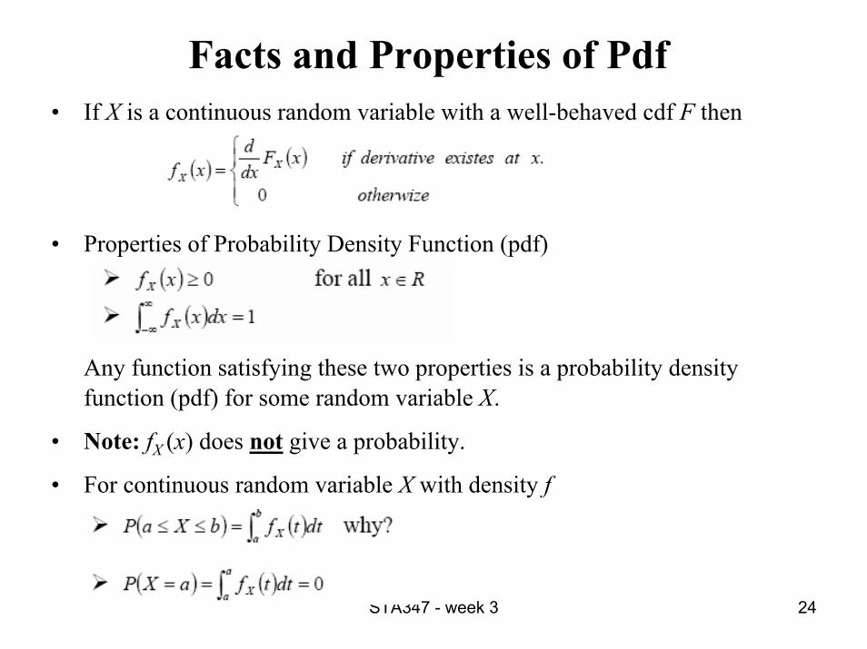
Facts and Properties of Pdf• If X is a continuous random variable with a well-behaved cdf F then

• Properties of Probability Density Function (pdf)

Any function satisfying these two properties is a probability density function (pdf) for some random variable X.

• Note: fX (x) does not give a probability.

• For continuous random variable X with density f

STA347 - week 3 25

The Exponential Distribution

• A random variable X that counts the waiting time for rare phenomena has Exponential(λ) distribution. The parameter of the distribution λ = average number of occurrences per unit of time (space etc.). The pdf of X is given by:

• Questions: Is this a valid pdf? What is the cdf of X?

• Note: The textbook uses different parameterization λ = 1/β.

• Memory-less property of exponential random variable:

STA347 - week 3 26

The Gamma distribution• A random variable X is said to have a gamma distribution with

parameters α > 0 and λ > 0 if and only if the density function of X is

where

• Note: the quantity г(α) is known as the gamma function. It has the following properties:– г(1) = 1– г(α + 1) = α г(α)– г(n) = (n – 1)! if n is an integer.

( ) ( )⎪⎩

⎪⎨

⎧∞≤≤

Γ=

−−

otherwise

xxexf

x

X

0

01

αλααλ

STA347 - week 3 27

The Beta Distribution

• A random variable X is said to have a beta distribution with parameters α > 0 and β > 0 if and only if the density function of X is

STA347 - week 3 28

The Normal Distribution• A random variable X is said to have a normal distribution if and only if,

for σ > 0 and -∞ < μ < ∞, the density function of X is

• The normal distribution is a symmetric distribution and has two parameters μ and σ.

• A very famous normal distribution is the Standard Normal distribution with parameters μ = 0 and σ = 1.

• Probabilities under the standard normal density curve can be done using Standard Normal Tables.

• Example:

STA347 - week 3 29

Summary of Discrete vs. Continuous Probability Spaces

• All probability spaces have 3 ingredients: (Ω, F, P)