random walk particle modelling of polymer …etd.lib.metu.edu.tr/upload/12621348/index.pdf ·...
TRANSCRIPT

RANDOM WALK PARTICLE MODELLING OF POLYMER INJECTION USING
MATLAB RESERVOIR SIMULATION TOOLBOX
A THESIS SUBMITTED TO
THE GRADUATE SCHOOL OF NATURAL AND APPLIED SCIENCES
OF
MIDDLE EAST TECHNICAL UNIVERSITY
BY
GÖKHAN MAMAK
IN PARTIAL FULFILLMENT OF THE REQUIREMENTS
FOR
THE DEGREE OF MASTER OF SCIENCE
IN
PETROLEUM AND NATURAL GAS ENGINEERING
SEPTEMBER 2017


Approval of the Thesis:
RANDOM WALK PARTICLE MODELLING OF POLYMER INJECTION
USING MATLAB RESERVOIR SIMULATION TOOLBOX
submitted by GÖKHAN MAMAK in partial fulfillment of the requirements for the
degree of Master of Science in Petroleum and Natural Gas Engineering Department,
Middle East Technical University by,
Prof. Dr. Gülbin Dural Ünver
Dean, Graduate School of Natural and Applied Sciences
Prof. Dr. Serhat Akın
Head of Department, Petroleum and Natural Gas Engineering
Asst. Prof. Dr. İsmail Durgut
Supervisor, Petroleum and Natural Gas Engineering Dept., METU
Examining Committee Members:
Prof. Dr. Mahmut Parlaktuna
Petroleum and Natural Gas Engineering Dept., METU
Asst. Prof. Dr. İsmail Durgut
Petroleum and Natural Gas Engineering Dept., METU
Asst. Prof. Dr. Emre Artun
Petroleum and Natural Gas Engineering Dept., METU NCC
Prof. Dr. Serhat Akın
Petroleum and Natural Gas Engineering Dept., METU
Assoc. Prof. Dr. Çağlar Sınayuç
Petroleum and Natural Gas Engineering Dept., METU
Date: 08.09.2017

iv
I hereby declare that all information in this document has been obtained and
presented in accordance with academic rules and ethical conduct. I also declare that,
as required by these rules and conduct, I have fully cited and referenced all material
and results that are not original to this work.
Name, Last name: Gökhan Mamak
Signature:

v
1ABSTRACT
RANDOM WALK PARTICLE MODELLING OF POLYMER INJECTION USING
MATLAB RESERVOIR SIMULATION TOOLBOX
Mamak, Gökhan
M.S., Department of Petroleum and Natural Gas Engineering
Supervisor: Asst. Prof. Dr. İsmail Durgut
September, 2017, 83 pages
Enhanced oil recovery (EOR) is essential to increase the maximum recoverable oil by
natural means of production. Having chosen an EOR method, the effectiveness of the
method should be analyzed before applying to a reservoir since the methods are generally
costly. Polymer injection is a chemical EOR process, where the injected polymer with
water increases the water viscosity, and help increasing the sweep efficiency in the
reservoir. In order to model the effects of polymer injection, the random-walk particle
tracking method is implemented on MATLAB Reservoir Simulation Toolbox (MRST),
an open source code for MATLAB for reservoir modelling. Our approach is to utilize the
random walk form of transport equation for the advection/diffusion of the injected
chemical in the porous medium whereas the continuity equations are solved by the black-
oil simulator MRST. Verification of MRST models integrity is done by comparing its
simple transport model with a known analytical solution, and its polymer model with
ECLIPSE 100 Black Oil Simulator’s results. Then the particle tracking method is applied
on one-dimensional and two-dimensional injection scenarios.
The method overcomes the numerical diffusion problem, which is a problem of finite
difference/finite volume discretization techniques. We can also use the method to model
the effect of dispersion coefficient, which is hard to obtain by normal methods. However,

vi
the random nature of the solution sometimes causes convergence problems in some two-
dimensional simulations.
Keywords: Enhanced oil recovery, polymer injection, particle tracking method, reservoir
modelling, dispersion

vii
2ÖZ
MATLAB REZERVUAR SİMÜLASYON EKLENTİSİ KULLANARAK
RASTLANTISAL PARÇACIK HAREKET METODU İLE POLİMER
ENJEKSİYONU MODELLEMESİ
Mamak, Gökhan
Yüksek Lisans, Petrol ve Doğal Gaz Mühendisliği Bölümü
Tez Yöneticisi: Yrd. Doç. İsmail Durgut
Eylül 2017, 83 sayfa
Geliştirilmiş petrol üretimi (EOR) doğal yollardan kurtarılabilecek maksimum petrol
miktarını arttırmak için gereklidir. EOR metodu seçildikten sonra, genellikle metotlar
yüksek yatırım gerektirdiğinden dolayı uygulamadan önce metodun etkenliği analiz
edilmelidir. Polimer enjeksiyonu, su ile birlikte enjekte edilen polimerin suyun
viskozitesini arttırdığı ve rezervuardaki süpürme veriminin arttırıldığı bir kimyasal EOR
metodudur. Polimer enjeksiyonunun etkilerini modellemek için düzensiz hareket
metodunu kullanarak parçacık izleme metodu, rezervuar modellemede kullanılan açık kod
MATLAB Reservoir Simulation Toolbox (MRST) üzerinde uygulanmıştır. Bu
yaklaşımımızda enjekte edilen kimyasalın gözenekli ortamda taşınma denklemi düzensiz
dağılım formunda çözülürken süreklilik denklemleri üç fazlı akışkan simülatörü MRST
tarafından çözülmektedir. MRST modellerinin tutarlılığı, içerdiği basit taşıma modelinin
bilinen bir analitik yöntemle ve polimer modelinin ECLIPSE 100 Black Oil Simulator’ün
sonuçlarıyla kıyaslanarak doğrulanmıştır. Sonrasında parçacık izleme metodu tek boyutlu
ve iki boyutlu enjeksiyon senaryoları üzerinde uygulanmıştır.
Metodun uygulaması sonlu kalan/sonlu hacim ayrıştırma tekniklerinin bir problemi olan
sayısal dağılım probleminin üstesinden gelmektedir. Metot ayrıca normal metotlarla elde

viii
edilmesi zor olan dağılım katsayısının etkilerinin gözlemlemek için de kullanılabilir.
Ancak çözümün rastlantısal doğası nedeniyle bazı iki boyutlu simülasyon senaryolarında
problemin bazen çözülememesine sebep olmaktadır.
Anahtar Kelimeler: Geliştirilmiş petrol üretimi, polimer enjeksiyonu, parçacık izleme
metodu, rezervuar modelleme, dağılım

ix
Don’t Panic

x
3ACKNOWLEDGEMENT
I would like to thank my supervisor Asst. Prof. Dr. İsmail Durgut for his continuous
support, valuable knowledge, and guidance throughout my thesis. Even when I do not feel
the same way, his continuous belief in my work and me kept me going and made this
thesis possible. I cannot thank you enough for the moral support and insight you gave me.
I also would like to thank İnanç Hıdıroğlu, my roommate and one of the best friends I
have, along with my brothers in the department, Berk Bal and Burak Parlaktuna. Their
presence and comfort they provide was the most valuable. All my colleagues and friends
in the department helped me with their support and good times we shared together.
I have to mention Tuğçe Özdemir’s knowledge and her study that gave me so much
guidance in the writing process. Thank you so much.
My chosen siblings Hilal Saat, Enes Sezer, Barışkan Süvari, and Selçuk Karagöz, who
were always there when I needed. You guys have tolerated me so much at my worst, have
been the best company that I could ever wish for. Sometimes I do not even think that I
deserve you. Thank you for being you and always having my back.
My grandfather Ayhan Mamak, I miss your voice the most.
Finally, my beloved parents Göksel Mamak and Can Mamak, whom I will never stop
trying to make proud. Thank you for being the best parents and believers that I have. I
love you so much. Then there is my sister, my little witch, my caster of lumos, Cansu
Mamak. You are the best thing that ever came into my life and my literal key that I will
always carry on me to open the toughest doors. I will never stop loving you and being
there for you.
There are a lot more names I want to thank but the pages will not be enough. Thank you
all for being in my life and making me the man that I am today.

xi
4TABLE OF CONTENTS
ABSTRACT ....................................................................................................................... v
ÖZ ................................................................................................................................... vii
ACKNOWLEDGEMENT ................................................................................................. x
TABLE OF CONTENTS .................................................................................................. xi
LIST OF FIGURES ........................................................................................................ xiv
LIST OF TABLES .......................................................................................................... xvi
NOMENCLATURE ...................................................................................................... xvii
CHAPTERS
1 INTRODUCTION ........................................................................................................ 1
2 ENHANCED OIL RECOVERY................................................................................... 5
2.1 Reservoir Recovery ............................................................................................. 5
2.2 Enhanced Oil Recovery ....................................................................................... 6
2.2.1 Thermal Methods ......................................................................................... 7
2.2.2 Miscible Methods ......................................................................................... 7
2.2.3 Chemical Methods ....................................................................................... 8
3 FLOW PARAMETERS & PROCESSES ..................................................................... 9
3.1 Permeability ......................................................................................................... 9
3.2 Mobility ............................................................................................................. 10
3.3 Diffusion & Dispersion ..................................................................................... 11
3.3.1 Diffusion .................................................................................................... 11
3.3.2 Dispersion .................................................................................................. 13
4 POLYMERS ............................................................................................................... 15

xii
4.1 Structure............................................................................................................. 15
4.2 Adsorption ......................................................................................................... 16
4.3 Effects on Mobility ............................................................................................ 18
5 MODELLING EQUATIONS ..................................................................................... 21
5.1 Black-Oil Model Equations ............................................................................... 21
5.2 Polymer Equations ............................................................................................. 22
6 MATLAB RESERVOIR SIMULATION TOOLBOX ............................................... 25
6.1 MRST Description ............................................................................................. 25
6.2 Buckley-Leverett Analytical Solution ............................................................... 26
6.3 Polymer Model of MRST .................................................................................. 28
7 PARTICLE MODEL ................................................................................................... 31
7.1 Random Walk Particle Model Description ........................................................ 31
7.2 Assumptions in the Model ................................................................................. 33
7.3 Movement of the Particles ................................................................................. 33
8 STATEMENT OF PROBLEM ................................................................................... 37
9 RESULTS & DISCUSSION ....................................................................................... 39
9.1 Verification of MRST Models ........................................................................... 39
9.1.1 Buckley-Leverett Verification .................................................................... 39
9.1.2 ECLIPSE Verification ................................................................................ 42
9.2 Numerical Dispersion ........................................................................................ 44
9.2.1 Water Flooding Problem ............................................................................ 44
9.2.2 1D Polymer Injection Problem ................................................................... 45
9.3 Implementation of Model into MRST ............................................................... 48
9.4 1D Problem ........................................................................................................ 49
9.4.1 Effect of Dispersion Coefficient ................................................................ 55

xiii
9.4.2 Effect of Particle Number Injected ............................................................ 58
9.5 2D Problem ........................................................................................................ 60
9.5.1 Velocity Field Interpolation ....................................................................... 60
9.5.2 1st Scenario ................................................................................................. 61
9.5.3 2nd Scenario ................................................................................................ 66
10 CONCLUSION ......................................................................................................... 73
REFERENCES ................................................................................................................. 75
APPENDICES
A CODE IMPLEMENTED ........................................................................................... 79
xiv
5LIST OF FIGURES
FIGURES
Figure 3.1 Field & Lab Dispersivities (Arya et al., 1988) ............................................... 14
Figure 4.1 Adsorption Curve (Sheng, 2011) ................................................................... 18
Figure 4.2 Areal Sweep Efficiency of Water Flooding (left) & Polymer Flooding (right)
(Sheng, 2011) ................................................................................................................... 19
Figure 4.3 Produced Concentration vs. Polymer Volume Injected (Gogarty, 1967) ...... 20
Figure 6.1 Fractional Flow Curve (Dake, 1998) ............................................................. 27
Figure 6.2 Buckley-Leverett Analytical Solution of Water Saturation Profile (Craft &
Hawkins, 1991) ................................................................................................................ 29
Figure 7.1 Particle Movement Represantation (Prickett, Naymik, & Lonnquist, 1981) . 32
Figure 9.1 Relative Permeability Curve .......................................................................... 40
Figure 9.2 Fractional Flow & Derivative ........................................................................ 40
Figure 9.3 Comparison of Flood Front Position .............................................................. 41
Figure 9.4 Comparison of Polymer Concentration Profiles ............................................ 43
Figure 9.5 Flood Front Movement with Different Grid Numbers .................................. 44
Figure 9.6 Viscosity Multiplier ....................................................................................... 46
Figure 9.7 Polymer Adsorption Curve ............................................................................ 46
Figure 9.8 Polymer Concentration Profile with Different Grid Numbers ....................... 47
Figure 9.9 Solution Flow Chart ....................................................................................... 49
Figure 9.10 MRST Polymer Concentration & Saturation Profiles ................................. 50
Figure 9.11 Particle Polymer Concentration & Saturation Profiles ................................ 52
Figure 9.12 1D Production Curve Comparisons ............................................................. 54
Figure 9.13 Effect of Dispersivity Coefficient on Polymer Concentration Movement .. 55
Figure 9.14 Effect of Dispersivity Coefficient ................................................................ 56
Figure 9.15 Polymer Concentration Profile with Different Number of Particles ........... 58
Figure 9.16 Effect of Velocity Field Interpolation on Particle Distribution, without
Interpolation (a), with Interpolation (b) ........................................................................... 60

xv
Figure 9.17 2D Concentration Distribution Comparison (1st Scenario), MRST (above),
Particle (below) ................................................................................................................ 62
Figure 9.18 Particle Distribution Profiles (1st Scenario) ................................................. 64
Figure 9.19 2D Production Curve Comparison (1st Scenario) ........................................ 65
Figure 9.20 2D Concentration Distribution Comparison (2nd Scenario), MRST (above),
Particle (below) ................................................................................................................ 67
Figure 9.21 Particle Distribution Profiles (2nd Scenario) ................................................ 69
Figure 9.22 2D Production Curve Comparison (2nd Scenario) ....................................... 70

xvi
6LIST OF TABLES
TABLES
Table 4.1 General Polymer Characteristics ..................................................................... 16
Table 9.1 One Dimensional Problem Properties ............................................................. 47
Table 9.2 Two Dimensional Problem 1st Scenario Properties ......................................... 61
Table 9.3 Two Dimensional Problem 2nd Scenario Properties ........................................ 66

xvii
7NOMENCLATURE
𝐴 Flow area, cm2
𝑏𝛼 Formation volume factor of phase 𝛼
C Concentration, mol/cm3 or kg/m3
𝐶𝑝 Injected polymer concentration, kg/m3
�̂�𝑝 Adsorbed polymer concentration, kg/m3
𝐷0 Diffusion coefficient, cm2/s
𝐷𝜏 Effective diffusion coefficient, cm2/s
𝐷𝐿 Longitudinal dispersion coefficient, cm2/s
𝐷𝑇 Transverse dispersion coefficient, cm2/s
𝐷𝐶 Dispersion coefficient used in the model, m2/s
𝑑𝑝 Average grain particle diameter, m2
𝐸 Overall displacement efficiency (oil recovered by process / oil in place at start of
process)
𝐸𝐷 Microscopic displacement efficiency
𝐸𝑉 Macroscopic displacement efficiency
F Flux, mol/s/cm2
𝐹𝑙 Inhomogeneity factor of the porous medium
𝐹𝑅 Formation electrical resistivity factor
𝑓𝑤 Fractional flow of water
𝑔 Gravitational acceleration factor m/s2

xviii
𝑘 Absolute permeability, Darcy
𝑘𝑟𝛼 Relative permeability of phase 𝛼
𝑘𝑒𝛼 Effective permeability of phase 𝛼, Darcy
𝐿 Length of the porous medium, m
𝑀 Mobility ratio
ℳ Polymer mass that can be adsorbed by unit mass of rock, kg/kg
𝑚𝑎𝑑𝑠 Mass of polymer that can be adsorbed by grid cell, kg
𝑚𝑟𝑒𝑑 Particle mass to be reduced due to adsorption, kg
𝑚𝑝 Mobile polymer mass in a grid cell, kg
𝑚𝜇 Viscosity multiplier function for polymer
𝑁 Moles of chemical injected, mol
𝒩 Number of particles in a cell
𝑃𝛼 Relative pressure of the phase 𝛼, Pa
𝑄 Volumetric flow rate, cm3/sec
𝑅𝑅𝐹 Residual resistance factor
𝑟𝑠 Solution gas oil ratio, scf/bbl
𝑟𝑣 Vaporized oil in gas phase, bbl/MMscf
𝑆𝛼 Saturation of phase 𝛼
𝑆𝑜𝑟 Residual oil saturation
𝑆𝑤𝑐 Connate water saturation

xix
𝑆𝑑𝑝𝑣 Dead pore volume
𝑡 Time, s
𝑉 Volume of a grid cell, m3
𝑣 Interstitial velocity, m/s
x Length, cm
∆𝑥𝑠𝑝𝑟𝑒𝑎𝑑 Spreading distance of particle due to diffusion and dispersion
𝛼𝐿 Longitudinal dispersivity, m
𝜇𝛼 Viscosity of phase 𝛼, cp
𝜇𝑤,𝑒𝑓𝑓 Effective water viscosity, cp
𝜇𝑝,𝑒𝑓𝑓 Effective polymer viscosity, cp
𝜇𝑓𝑚 Fully mixed polymer and water solution viscosity
𝜇𝑝𝑚 Partially mixed polymer and water solution viscosity
𝜆𝛼 Mobility of phase 𝛼
𝜏 Tortuosity
Φ Porosity
𝜎2 Variance of Gaussian distribution
𝜌𝛼 Density of phase 𝛼, kg/m3
𝜌𝑟𝑜𝑐𝑘 Density of rock, kg/m3

xx

1
CHAPTER 1
1INTRODUCTION
Hydrocarbon reservoir performance under different conditions can be predicted through
reservoir simulation, which combines physics, mathematics, reservoir engineering, and
computer programming. Reservoir simulation is needed to forecast reservoir performance
accurately because of the fact that the investments done on recovery projects may require
high costs, and the risks of the development program should be evaluated and minimized.
A set of partial differential equations (PDE) are developed and solved under reservoir’s
initial and boundary conditions. The main advantage of this approach is to have minimum
amount of simplifying assumptions in the reservoir. The PDE’s are discretized with finite-
difference method in general (Ertekin, Abou-Kassem, & King, 2001). However, the
transport equations solved introduces a numerical dispersion as Kinzelbach (1990) stated.
Polymer injection is an enhanced oil recovery (EOR) method used primarily to increase
the injected solutions viscosity and improve sweep efficiency (Sheng, 2011). Accurate
modelling of polymer injection programs are required as other recovery methods in the
industry.
Zheng & Wang (1999) states in the user guide of MT3DMS, a modular multispecies
transport model used in groundwater systems, that the numerical dispersion is an effect
similar to physical dispersion in a system. However, numerical dispersion is introduced
by truncation errors when solving the continuity equations in simulators. As stated in

2
CMG (2010) user guide, a commercial advanced process and thermal reservoir simulator
CMG STARS, even in uniform reservoir models, numerical dispersion introduces errors
in simulation results.
A random-walk particle tracking method can be used in order to model the effects of an
injection process. The method does not require numerical solutions of PDE’s (Liu,
Bodvarsson, & Pan, 2000). The transport process of particles is solved as a linear equation.
The solution therefore is virtually free of numerical dispersion effects (Zheng & Wang,
1999). In summary, the method calculates randomly injected/distributed equal mass
particles’ position representing a chemical in a system. Particle masses along with their
position information can be used to calculate concentration and add the effects of the
chemical to the system.
Random-walk particle tracking method can be used in different flow problems, as it is
easy to apply and modify. The method is used to model the advection and
diffusion/dispersion of chemicals in different studies. Kinzelbach (1990) used the method
to simulate pollutant transport in groundwater for instance. Inoue, Takao, & Tanaka
(2009) applies the method to delineate the capture zones in groundwater supply wells. Liu
et al. (2000) used the method to model solute transport, while Stalgorova & Babadagli
(2012) applies the method for tracer injection in fractured porous media. Method is used
to investigate mixing in miscible displacements of tracer floods by John, Lake, Bryant, &
Jennings (2010). Özdemir (2015) used the method to model marine sediment pollution by
comparing the method with analytical and finite-difference models.

3
In this study, a particle method is implemented in MATLAB Reservoir Simulation
Toolbox (MRST), an open source code for reservoir simulation, in order to simulate the
effects of polymer injection. The thesis develops as:
Definition of enhanced oil recovery
Definition of some flow parameters & processes
Information on polymers
Information on general modelling equations
Introduction of MATLAB Reservoir Simulation Toolbox and its verification
Information on the developed particle model
Statement of the problem
Results and discussion
Conclusion

4

5
CHAPTER 2
2 ENHANCED OIL RECOVERY
In this chapter, definitions of petroleum recovery processes and Enhanced Oil Recovery
(EOR) methods are explained briefly.
2.1 Reservoir Recovery
A petroleum reservoir can be described as a porous and permeable medium that contains
oil, gas and brine, which can be produced by numerous recovery techniques. Oil recovery
processes from a reservoir is divided into three groups: primary, secondary, and tertiary
or enhanced oil recovery.
1. Primary recovery is the oil displacement process generally based on reservoir’s
natural energy. This energy is the pressure difference generated between reservoir
and production well from numerous forces such as, natural gas expansion,
gravitational force, water encroachment, and rock expansion. These forces can
occur at the same time, or consecutively depending on the reservoir properties.
2. Secondary recovery processes start after the pressure difference between reservoir
and production well is lowered due to primary recovery processes and is not
enough. Reservoir pressure is partially increased by means of injecting water or
gas into the reservoir with injection wells. Injected water or gas forces the oil in
the reservoir to flow towards production wells and sweeps the reservoir.

6
3. Enhanced oil recovery (EOR) starts after waterflooding and gas injection
processes depleted the reservoir. The EOR processes are divided into three
categories: thermal, miscible and chemical (Donaldson, Chilingarian, & Yen,
1989).
2.2 Enhanced Oil Recovery
The term Enhanced Oil Recovery includes processes of injection of gases or liquid
chemicals and use of thermal energy. Since some reservoirs may need EOR processes to
start production, the term tertiary recovery is replaced by EOR. Aim of EOR is to provide
extra energy to reservoir’s natural energy and displace the oil remained. Additionally,
reservoir conditions are changed favorably for oil flow with the interactions of injected
fluids and rock/oil system. The displacement efficiency of the process is the product of
macroscopic and microscopic efficiencies.
𝐸 = 𝐸𝐷𝐸𝑉 (2.1)
where:
𝐸 = overall displacement efficiency (oil recovered by process / oil in place at start of
process)
𝐸𝐷 = microscopic displacement efficiency
𝐸𝑉 = macroscopic displacement efficiency
Microscopic displacement efficiency is the process’s ability to mobilize the oil at the pore
scale. It is considered in the rock surface reached by the displacing fluid and is the
measurement of displacement capacity in that area. Macroscopic displacement efficiency
is the capacity of the injected fluid to sweep the oil in the reservoir volume towards
production wells, both areally and vertically (Green & Willhite, 1998).
There is also the concept of Microbial Enhanced Oil Recovery (MEOR) present in the
literature. In MEOR methods, microbes are injected in a reservoir in order to improve the
oil recovery. Through microbial action in the reservoir, chemicals that can enhance the

7
recovery are produced in reservoir. Different mechanisms can occur in a reservoir such as
viscosity reduction by produced gas, water viscosity increase by biopolymers etc.
(Lacerda, Priimenko, & Pires, 2012).
Before selecting an EOR method, careful analysis of the reservoir is needed. Reservoir
rock type, oil saturations, drive mechanisms should be studied to select the most efficient
EOR method and should be continuously monitored during operations. The three main
types of methods are explained below:
2.2.1 Thermal Methods
For reservoirs with low gravity, high viscosity oil and high porosity, thermal methods are
used. The idea is to create or apply heat energy in the reservoir to increase oil mobility. In
other words, increasing reservoir temperature decreases oil viscosity, in turn, increases its
mobility. In-situ combustion, wet combustion, and steam injection methods are used and
they are counted as thermal EOR methods. In-situ combustion involves burning the crude
oil near injection well and moving the burning zone through production wells with air
injection. Wet combustion method is essentially an in-situ combustion process. Water is
injected with air behind the burning zone to use the heat left behind the zone to create
superheated steam and evaporation front and decrease the amount of residual oil. Steam
injection is done either continuously or in cycles to achieve lower viscosities in the
reservoir. While both injection and production wells are used in continuous steam
injection, one well is used to inject steam and produce oil in cyclic injection (Donaldson
et al., 1989).
2.2.2 Miscible Methods
In miscible EOR methods, a solvent that can dissolve the reservoir fluids and create a
mixture that needs lower capillary forces to flow in the reservoir. Alcohols, refined
hydrocarbons, condensed hydrocarbon gases, liquefied petroleum gases, or carbon
dioxide are used in miscible floods. Injected fluid is followed by water or gas to push the
solvent-oil mixture towards production wells. In some processes, a fluid that is miscible

8
with both oil and water is used to create a single phase flowing in the reservoir (Donaldson
et al., 1989).
2.2.3 Chemical Methods
Chemical EOR methods focus on mobility control in the reservoir. Chemical EOR
processes include alkaline, surfactant, polymer and combinations of these chemicals
injection to the reservoir. In surfactant injection, chemicals reduce the interfacial tension
(IFT) between oil and displacing fluid. The effect of IFT is evaluated through the
dimensionless capillary number, which relates viscous forces and capillary forces. The
number is proportional with fluid viscosity and flow velocity, whereas inversely
proportional to IFT and reservoir porosity (Dandekar, 2013). Capillary number is
increased with reduced IFT and residual oil saturation decreases with the improved sweep
efficiency. Alkaline injection method is based on applying surfactant to reduce IFT in
reservoir conditions with chemical reactions between alkali and acids present in the
reservoir. Polymer injection’s main intention is to increase displacing phase viscosity and
increase oil mobility (Sheng, 2011). Injected polymer’s effects on reservoir and flow will
be discussed in Chapter 4.

9
CHAPTER 3
3FLOW PARAMETERS & PROCESSES
In this chapter, some flow parameters and processes will be presented in order to develop
a better understanding on polymer injection and model used.
3.1 Permeability
Permeability is the porous medium’s capacity to transmit fluids. It can be measured by
flow experiments in a reservoir rock. When the reservoir rock is 100% saturated with a
fluid, the measured permeability is called the absolute permeability of the rock. It is a rock
property and does not vary with fluid present in the reservoir. A French civil engineer,
Henry Darcy’s experiments on water flow through sand filters helped him to create the
mathematical expressions that is used to calculate the absolute permeability. The general
Darcy equation for fluid flow to calculate absolute permeability is given as:
𝑄 = −𝑘
𝜇𝐴
𝑑𝑃
𝑑𝐿
(3.1)
where:
𝑄 = Volumetric flow rate, cm3/sec
𝑘 = Absolute permeability, Darcy
𝜇 = Viscosity of fluid, cp

10
𝐴 = Flow area, cm2
𝑑𝑃 = Pressure difference between upstream and downstream, atm
𝑑𝐿 = Length of fluid flow, cm
The experiment and the formula used is based on some assumptions. The fluid is
incompressible, horizontal, steady state, under laminar regime, and there is no reaction
between the rock and fluid. However, reservoirs with a single-phase fluid rarely exists.
Therefore, concept of effective permeability is needed to calculate flow. When there are
more than one fluid flowing in the reservoir, flow of one phase affects the others. In such
reservoirs, permeability is generally specified as relative permeability, kr, which is defined
usually by the ratio between effective permeability, ke, of one phase to the absolute
permeability of the rock.
𝑘𝑟 =𝑘𝑒
𝑘
(3.2)
Relative permeability also depends on fluid saturations in the rock, wetting characteristics
of the fluids, and pore geometry. Relative permeability values of phases are given as a
table or plotted at different saturation rates, which generally ranges between irreducible
wetting-phase saturation and corresponding wetting-phase saturation of residual oil
saturation, in general (Dandekar, 2013).
3.2 Mobility
Mobility, 𝜆, of a phase in a reservoir is defined as the ratio between the effective
permeability, 𝑘𝑒, and viscosity, 𝜇, of the phase. It can also be defined as relative mobility,
using relative permeability of the phase.
𝜆 = 𝑘
𝜇
(3.3)
Mobility ratio, M, is the ratio between the displacing phase and displaced phase mobilities,
𝜆𝑢 and 𝜆𝑑, respectively. A mobility ratio lower than one is desirable for a displacement
process. Mobility control is an essential part of an EOR process. In processes such as

11
polymer flooding, mobility ratio of the displacing fluid is lowered to increase oil
production. In such cases, summation of the mobilities of displacing fluids, and displaced
fluids are used to calculate total mobilities. Mobility ratio is also defined as the total
mobility ratio and is desired to be lower than one. (Sheng, 2011).
𝑀 = ∑ 𝜆𝑢
∑ 𝜆𝑑
(3.4)
3.3 Diffusion & Dispersion
3.3.1 Diffusion
Diffusion is an important transport mechanism in reservoirs. Diffusion is defined as the
mixing of a material in a single phase in the absence of mechanical or convective mixing
(Sheng, 2011). Pressure gradients, temperature gradients, and concentration gradients in
a mixture can cause diffusion. Diffusion caused by concentration differences is called the
molecular diffusion. Fick’s law describes the concentration gradient flux of a material as:
𝐹 = −𝐷0
𝜕𝐶
𝜕𝑥
(3.5)
where:
F = Flux (mol/s/cm2)
𝐷0 = Diffusion coefficient (cm2/s)
C = Concentration (mol/cm3)
x = Length (cm)
In the porous medium, flow takes place in a tortuous path. Tortuosity of the medium is
the ratio, 𝜏, between the actual path length traveled by a fluid parcel and a single-line
distance of the same path. To add the effect of tortuosity, the diffusion coefficient, 𝐷0, is
changed with effective diffusion coefficient, 𝐷𝜏. The relationship between 𝐷𝜏 and 𝐷0 is:

12
𝐷𝜏 = 𝐷0
𝜏2
(3.6)
Tortuosity can also be defined in terms of electrical formation resistivity factor of the
medium, FR, which is the ratio between electrical resistivity of the medium with a fluid
that conducts electricity and the fluid in the medium, and porosity, Φ.
𝜏2 = 𝐹𝑅Φ (3.7)
Empirical relationship between FR and 𝛷 by Archie’s law is:
𝐹𝑅 = Φ−𝑛 (3.8)
The exponent n varies from 1.4 to 2.0. When n is taken to be 2, effective diffusion
coefficient becomes:
𝐷𝜏 = 𝐷0Φ (3.9)
When mass balance in a small porous medium is written in one dimension, diffusion can
be profiled as:
𝜕𝐶
𝜕𝑡= 𝐷𝜏
𝜕2𝐶
𝜕𝑥2
(3.10)
Equation 3.10 is known as the Fick’s second law of diffusion.
Molecular diffusion results from the random motion of the molecules in a solution. Hence,
it can be represented statistically. In a system with no chemical injected before t = 0, when
N moles of chemical is injected at origin x = 0, concentration profile can be calculated
with the stated function below (Sheng, 2011):
𝐶(𝑥, 𝑡) = 𝑁
√4𝜋𝐷0𝑡exp (−
𝑥2
4𝐷0𝑡)
(3.11)
𝐶(𝑥, 𝑡) is in mol/cm. Concentration of the chemical is equal to 0 except at the origin at
time t = 0. At the origin C→ ∞. Equation 3.11 is similar to Gaussian distribution function
(Sheng, 2011),
𝑛(𝑥) =𝑁
√2𝜋𝜎2exp (−
𝑥2
2𝜎2)
(3.12)

13
𝜎2 is the variance of the distribution. Using the similarity between equations 3.11 and
3.12, diffusion coefficient can be related with variance as:
𝜎2 = 2𝐷0𝑡 (3.13)
Statistics states that the mean diffusion length can be estimated. The equation 3.14
represents distance traveled by the 68% of the original mass (Sheng, 2011).
𝜎 = √2𝐷0𝑡 (3.14)
3.3.2 Dispersion
In reservoir fluid flow, changes in velocity of the flow causes an uneven mixing of the
chemicals. Added effect of gross fluid flow in chemical mixing or concentration gradients
caused by the phenomena is called dispersion. Two types of dispersion is defined as the
longitudinal dispersion, DL, and the transverse dispersion, DT. Longitudinal dispersion is
the dispersion in gross fluid flow direction, whereas transverse dispersion is in transverse
direction of it.
Dispersion is a highly scale dependent parameter, therefore quantifying is hard and done
experimentally or empirically. Empirical correlation describes DL as sum of molecular
diffusion and convective dispersion components. Perkins & Johnston (1963) gives the
correlation between DL and 𝐷0, based on the experiments held on different grain particle
sized samples in the literature, as:
𝐷𝐿
𝐷0=
1
𝐹𝑅Φ+ 0.5
𝑣𝐹𝑙𝑑𝑝
𝐷0
(3.15)
For 𝑣𝐹𝑙𝑑𝑝/𝐷0 < 50, which is the effective ratio for diffusion to equalize the concentration
in pore spaces, where:
𝑣 = Interstitial velocity, m/s
𝐹𝑙 = Inhomogeneity factor of the porous medium
𝑑𝑝 = Average grain particle diameter, m2

14
When the convective term is high, dispersion coefficient and velocity are proportional.
When 𝐹𝑙, 𝑑𝑝, and 𝐷0 are assumed constants in a reservoir, dispersivity parameter, αL, can
be defined:
𝛼𝐿 =𝐷𝐿
𝑣
(3.16)
Experimental and field data on the literature on longitudinal dispersivity is shown in
Figure 3.1 and correlations are reported by Arya, Hewett, Larson, & Lake (1988) for field
data and all data respectively as:
𝛼𝐿 = 0.229𝐿0.755 (3.17)
𝛼𝐿 = 0.044𝐿1.13 (3.18)
Figure 3.1 Field & Lab Dispersivities (Arya et al., 1988)
Transverse dispersion and dispersivity are studied less in the literature and their effects
are much less then longitudinal dispersion and dispersivity (Sheng, 2011).

15
CHAPTER 4
4POLYMERS
In this chapter, general information about polymers is given. Their structure, effect on
flood conditions and adsorption is discussed.
4.1 Structure
Rodriguez et al. (1993) states the polymer molecules dissolve in water via hydrogen
bonding. Molecules dissolve in water but hold some of their structural identity in solution.
Coils of polymer molecules holds large volumes of solvent. The connected coils deform
and change shape under applied pressure, and drags other coils and solvent with them
during flood. General polymer structures are given in Table 4.1. Sheng (2011) gives the
good polymer properties as:
Thermally stable (no hydroxyl group (-O-) in the carbon chain)
Low adsorption rate on rock surface (negative ionic hydrophilic group)
Good viscosifying powder
Chemically stable (nonionic hydrophilic group)
The mostly used polymers are the synthetic type, hydrolyzed polyacrylamide (HPAM).

16
Table 4.1 General Polymer Characteristics
Structure Characteristics Sample Polymers
-O- in the backbone Low thermal stability,
thermal degradation at high
T, only suitable at <80℃
Polyoxyethylene, sodium
alginate, sodium
carboxymethyl cellulose,
HEC, xanthan gum
Carbon chain in the
backbone
Good thermal stability,
degradation not severe at
<110℃
Polyvinyl, sodium
polyacrylate,
polyacrylamide, HPAM
-COO- chain in
hydrophilic group
Good viscosifier, less
adsorption on sandstones
due to the repulsion
between chain links, but
precipitation with Ca2+ and
Mg2+, less chemical
stability
Sodium alginate, sodium
carboxymethyl cellulose,
HPAM, xanthan gum
-OH or –CONH2 in
hydrophilic group
No precipitation with Ca2+
and Mg2+, good chemical
stability, but no repulsion
between chain links, thus
less viscosifying powder,
high adsorption due to
hydrogen bond formed on
sandstone rocks
Polyvinyl, HEC,
polyacrylamide, HPAM
Source: (Sheng, 2011)
4.2 Adsorption
Adsorption is the phenomena that is caused by the interaction between polymer molecules
and rock surface. Because of van der Waals forces and hydrogen bonding, molecules are
bound to rock surface. Adsorption is the most important retention mechanism in the

17
reservoir because it is a major property of the solution-rock system. The process depends
on the rock surface area exposed to the polymer solution. The other retention mechanisms
are called mechanical entrapment and hydrodynamic retention. Since it is hard to
distinguish the mechanisms, the term adsorption is generally used for retention and
polymer loss. In general, mass of polymer adsorbed by the unit mass of rock is used as a
unit for adsorption. To describe polymer adsorption, the Langmuir-type isotherm is used
(Sheng, 2011):
�̂�𝑝 = min (𝐶𝑝,𝑎𝑝(𝐶𝑝 − �̂�𝑝)
1 + 𝑏𝑝(𝐶𝑝 − �̂�𝑝))
(4.1)
where:
�̂�𝑝 = Adsorbed polymer concentration
𝐶𝑝 = Injected polymer concentration
𝐶𝑝 − �̂�𝑝 = Equilibrium concentration of the solution-rock system
𝑎𝑝, 𝑏𝑝 = Empirical constants
However, this isotherm is used when adsorption process is reversible. It means that the
concentration in the reservoir can increase by desorption of polymer molecules from the
rock surface in time. In general, adsorption is accepted irreversible. Although small
amounts can be recovered from rock surface with continuous water or brine injection, the
recovery is not enough to calculate concentration properly. In other words, retention by
adsorption is much higher than polymer removal. Therefore, if the process is taken to be
irreversible as discussed, another parameter, �̂�𝑝,𝑚𝑎𝑥, is added for observing the adsorption
history.
�̂�𝑝,𝑚𝑎𝑥 = 𝑚𝑎𝑥 {(�̂�𝑝)1
, (�̂�𝑝)2
, … , (�̂�𝑝)𝑛
} (4.2)
Time steps are indicated with number 1, 2, …, n where the current time step is n. �̂�𝑝,𝑚𝑎𝑥
cannot exceed the adsorption capacity. A typical adsorption curve can be seen on Figure
4.1 (Sheng, 2011).

18
Figure 4.1 Adsorption Curve (Sheng, 2011)
4.3 Effects on Mobility
Use of polymer solutions may increase the oil displacement efficiency in a reservoir. The
increment in the efficiency rate is the result of lowered displacing phase mobility.
Lowered mobility ratio causes the areal sweep efficiency and vertical coverage to
improve. The mobility cut can be done by lowering permeability, increasing solution
viscosity, or a combination of both (Rodriguez et al., 1993). The overall macroscopic
displacement efficiency of polymer flooding over waterflooding can be seen on Figure
4.2.
Polymer solutions show higher resistance to flow than regular waterflooding. Hence, the
mobility of the displacing phase is lowered and mobility ratio becomes more favorable.
This resistance is caused by the swelled polymer molecules in a good solvent. The effect
is greater with higher molecular weight of polymer. (Mungan, Smith, & Thompson, 1966).
Polymer effect on solution viscosity increases with polymer concentration in solution.
Effective water viscosity can be defined with Todd-Longstaff mixing model, which
involves mixing rate of polymer and water, and viscosity multiplier function of solution
with complete mixing (Bao et al., 2016).

19
Figure 4.2 Areal Sweep Efficiency of Water Flooding (left) & Polymer Flooding (right)
(Sheng, 2011)
Gogarty (1967) states that the permeability reduction mechanism is more complicated. In
the core-plug displacement experiments with 1200-ppm polymer solution, similar results
with Figure 4.3 is realized. No polymer is produced until 1 pore volume (PV) of polymer
solution is injected. Produced polymer concentration within the core is equal with the
injection concentration after approximately 8 PV of injection is carried out. Late
equalization means that polymer retention takes place in the porous medium during the
flooding. Polymer retention is caused by the entrapment of polymer molecules in smaller
pore openings and adsorption on the rock surfaces. Adsorption continues until the
equalization in the concentration is completed. Since, effective viscosities decrease with
the effect of polymer retention and permeability reduction, polymer flooding should be
done with low adsorption rate.

20
Figure 4.3 Produced Concentration vs. Polymer Volume Injected (Gogarty, 1967)
The interfacial viscosity between polymer and oil also plays an important role in polymer
flooding. Higher interfacial viscosity and shear stress between polymer and oil causes the
polymer to have larger pull force on oil droplets. This effect helps pushing and pulling of
oil droplets in dead-ends of porous medium. Higher push-pull force on oil droplets helps
reducing the residual oil saturation, 𝑆𝑜𝑟 (Sheng, 2011).

21
CHAPTER 5
5MODELLING EQUATIONS
This chapter summarizes the equations solved in polymer flood modelling.
5.1 Black-Oil Model Equations
Black-oil simulators are three phase simulators (i.e. oil, water and gas phases). This type
of simulators defines the hydrocarbon fluids as oil and gas phases, being combined
considered as combination of different weights of hydrocarbon components, which are
not individually involved in the model. Depending on the reservoir pressure and
hydrocarbon properties, the phases can be dissolved in each other either completely or
partially at the reservoir conditions. There is also the aqueous phase of water present.
Models used in this study defines boundaries of the reservoir as no-flow boundaries. The
initial state of the reservoir, reservoir rock and fluid properties are input to the model
manually. Bao et al. (2016) gives the continuity equations solved for the phases as:
𝜕𝑡(Φ𝑏𝑤𝑆𝑤) + ∇(𝑏𝑤𝜐𝑤) − 𝑏𝑤𝑞𝑤 = 0 (5.1)
𝜕𝑡[Φ(𝑏𝑜𝑆𝑜 + 𝑏𝑔𝑟𝑣𝑆𝑔)] + ∇(𝑏𝑜𝜐𝑜 + 𝑏𝑔𝑟𝑣𝜐𝑔) − (𝑏𝑜𝑞𝑜 + 𝑏𝑔𝑟𝑣𝑞𝑔) = 0 (5.2)
𝜕𝑡[Φ(𝑏𝑔𝑆𝑔 + 𝑏𝑜𝑟𝑠𝑆𝑜)] + ∇(𝑏𝑔𝜐𝑔 + 𝑏𝑜𝑟𝑠𝜐𝑜) − (𝑏𝑔𝑞𝑔 + 𝑏𝑜𝑟𝑠𝑞𝑜) = 0 (5.3)
𝑆𝑜 + 𝑆𝑔 + 𝑆𝑤 = 1 (5.4)
where 𝑏𝛼 denotes the formation volume factors. 𝑟𝑠 is the solution gas oil ratio and 𝑟𝑣 is the
vaporized oil in gas phase in the reservoir. Darcy’s law gives the phase fluxes as:

22
𝜐𝛼 = −𝜆𝛼𝑘(∇𝑃𝛼 − 𝜌𝛼𝑔∇𝑧) (5.5)
5.2 Polymer Equations
MATLAB Reservoir Simulation Toolbox (MRST) is used in this study to model polymer
flow in the reservoir. More information about MRST will be given in Chapter 7. The
model assumes that the polymer is only present in the aqueous phase and do not interfere
with hydrocarbon phases in the reservoir. Polymer properties such as the mixing
parameter, adsorption values of polymer etc. are given to the model along with the initial
reservoir conditions by the user. The continuity equation for the polymer is stated as (Bao
et al., 2016):
𝜕𝑡(Φ(1 − 𝑆𝑑𝑝𝑣)𝑏𝑤𝑆𝑤𝑐) + 𝜕𝑡(𝜌𝑟𝑐𝑎(1 − Φ)) + ∇(𝑏𝑤𝜐𝑝𝑐) − 𝑏𝑤𝑞𝑤𝑐 = 0 (5.6)
where:
𝑐𝑎 = Polymer adsorption concentration
𝜌𝑟 = Reservoir rock density, kg/m3
𝑆𝑑𝑝𝑣 = Dead pore volume (inaccessible pore space by polymer due to its larger molecular
size than some pore diameters)
Equations solved adds the effect of the viscosity change and permeability reduction to the
reservoir by means of polymer concentration in each grid block. Effective viscosity should
be applied in the phase flux equations to add these effects. In polymer solution model,
Darcy equations for water and polymer become:
𝜐𝑤 = −𝑘𝑤𝑆𝑤
𝜇𝑤,𝑒𝑓𝑓(𝑐)𝑅𝑘(𝑐)𝑘(∇𝑃𝑤 − 𝜌𝑤𝑔∇𝑧)
(5.7)
𝜐𝑝 = −𝑘𝑤𝑆𝑤
𝜇𝑝,𝑒𝑓𝑓(𝑐)𝑅𝑘(𝑐)𝑘(∇𝑃𝑤 − 𝜌𝑤𝑔∇𝑧)
(5.8)
The function 𝑅𝑘(𝑐) defined in these equations represents the permeability reduction effect
due to polymer adsorption and it is stated as:

23
𝑅𝑘(𝑐, 𝑐𝑚𝑎𝑥) = 1 + (𝑅𝑅𝐹 − 1)𝑐𝑎(𝑐, 𝑐𝑚𝑎𝑥)
𝑐𝑚𝑎𝑥𝑎
(5.9)
𝑐𝑚𝑎𝑥(𝑥, 𝑡) = max𝑠≤𝑡
𝑐(𝑥, 𝑠) (5.10)
𝑐𝑚𝑎𝑥𝑎 is the maximum polymer concentration adsorbed and RRF (residual resistance
factor) is the ratio between water relative permeability before and after polymer flood.
Both of these qualities depend on the rock type.
The effect of viscosity change is calculated with the help of Todd-Longstaff mixing
model. Displacement scenario and heterogeneity of the formation changes the Todd-
Longstaff mixing parameter, ω. Complete mixing is defined as ω = 1, whereas complete
segregation is ω = 0. Fully mixed solution viscosity can be defined as (Bao et al., 2016):
𝜇𝑓𝑚 = 𝑚𝜇(𝑐)𝜇𝑤 (5.11)
𝑚𝜇 is the viscosity multiplier function. Effective polymer viscosity is calculated by:
𝜇𝑝,𝑒𝑓𝑓 = 𝜇𝑓𝑚𝑤𝜇𝑝
1−ω (5.12)
Viscosity of a partially mixed solution, 𝜇𝑝𝑚, and effective water viscosity are calculated
as follows:
𝜇𝑝𝑚 = 𝜇𝑓𝑚𝑤𝜇𝑤
1−ω (5.13)
Then the effective water viscosity is calculated by summing the polymer solution and pure
water contributions as:
1
𝜇𝑤,𝑒𝑓𝑓=
1 − 𝑐̅
𝜇𝑝𝑚+
𝑐̅
𝜇𝑝,𝑒𝑓𝑓
(5.14)
𝜇𝑤,𝑒𝑓𝑓 =𝑚𝜇(𝑐)ω𝜇𝑤
1 − 𝑐̅ + 𝑐̅/𝑚𝜇(𝑐∗)1−ω
(5.15)
where 𝑐̅ = 𝑐/𝑐∗ and 𝑐∗ is the maximum possible polymer concentration (Bao et al., 2016).

24

25
CHAPTER 6
6MATLAB RESERVOIR SIMULATION TOOLBOX
MATLAB Reservoir Simulation Toolbox (MRST), solution method of its polymer model
and is explained in this chapter. Theory on Buckley-Leverett waterflooding is also given
for the simple verification of the toolbox.
6.1 MRST Description
MRST is an open-source code developed by SINTEF Applied Mathematics in Oslo. It is
not a simulator, but a fast prototyping and demonstration tool for new methods and
concepts for reservoir modelling, working with MATLAB. There are several modules for
basic reservoir characterization and flow functions. For cases that are more specific many
add-on modules can be activated for different physical models, solvers, etc. (Sintef, n.d.-
a)
In this thesis, the objective is to modify the source code of MRST to implement random
movement particle tracking method to the system. Before implementing the method,
integrity of MRST solutions is compared first by comparing MRST water flood solution
with analytical Buckley-Leverett solution, then MRST 1D polymer flood solution with
ECLIPSE solution of the same data.

26
6.2 Buckley-Leverett Analytical Solution
Before implementing the particle tracking method to MRST, integrity of MRST solutions
is checked as stated before. One of the verification tools used was the analytical Buckley-
Leverett solution of simple water flooding problem.
As Dake (1998) mentioned, distance from injection well of any water saturation, 𝑆𝑤, at
any time can be calculated in waterflooding applications. The equation is known as the
Buckley-Leverett or frontal-advance equation. Darcy equation can be written for both
water and oil phases respectively as:
𝑞𝑤 = −𝑘𝑘𝑤𝐴
𝜇𝑤(
𝜕𝑃𝑤
𝜕𝑥+
𝜌𝑤𝑔 sin 𝜃
1.0133 𝑥 106)
(6.1)
𝑞𝑜 = −𝑘𝑘𝑜𝐴
𝜇𝑜(
𝜕𝑃𝑜
𝜕𝑥+
𝜌𝑜𝑔 sin 𝜃
1.0133 𝑥 106)
(6.2)
𝑞𝑡 = 𝑞𝑤 + 𝑞𝑜 (6.3)
where:
𝑃𝛼 = Relative pressure of the phase, Pa
𝜌𝛼 = Density of the phase, kg/m3
𝑔 = Gravitational constant, m2/s
𝜃 = Flow angle
When the relation in Equation 6.3 is applied, 𝑞𝑤 can be written as:
𝑞𝑤 = − (𝜇𝑤
𝑘𝑘𝑤+
𝜇𝑜
𝑘𝑘𝑜) =
𝑞𝑡𝜇𝑜
𝑘𝑘𝑜+ 𝐴 (
𝜕𝑃𝑐
𝜕𝑥−
∆𝜌𝑔 sin 𝜃
1.0133 𝑥 106)
(6.4)
where the capillary pressure gradient is:
𝜕𝑃𝑐
𝜕𝑥=
𝜕𝑃𝑜
𝜕𝑥−
𝜕𝑃𝑤
𝜕𝑥
(6.5)
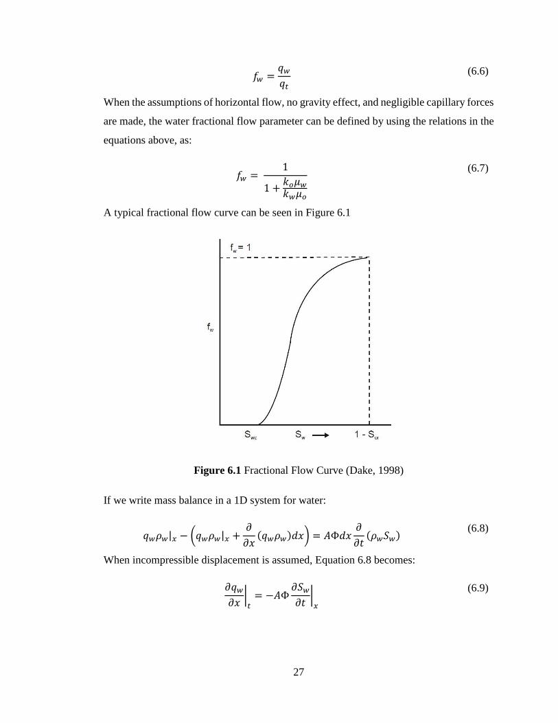
Fractional flow of water in the reservoir is:
27
𝑓𝑤 =𝑞𝑤
𝑞𝑡
(6.6)
When the assumptions of horizontal flow, no gravity effect, and negligible capillary forces
are made, the water fractional flow parameter can be defined by using the relations in the
equations above, as:
𝑓𝑤 = 1
1 +𝑘𝑜𝜇𝑤
𝑘𝑤𝜇𝑜
(6.7)
A typical fractional flow curve can be seen in Figure 6.1
Figure 6.1 Fractional Flow Curve (Dake, 1998)
If we write mass balance in a 1D system for water:
𝑞𝑤𝜌𝑤|𝑥 − (𝑞𝑤𝜌𝑤|𝑥 +𝜕
𝜕𝑥(𝑞𝑤𝜌𝑤)𝑑𝑥) = 𝐴Φ𝑑𝑥
𝜕
𝜕𝑡(𝜌𝑤𝑆𝑤)
(6.8)
When incompressible displacement is assumed, Equation 6.8 becomes:
𝜕𝑞𝑤
𝜕𝑥|
𝑡= −𝐴Φ
𝜕𝑆𝑤
𝜕𝑡|
𝑥
(6.9)

28
Differential of water saturation is:
𝑑𝑆𝑤 =𝜕𝑆𝑤
𝜕𝑥|
𝑡𝑑𝑥 +
𝜕𝑆𝑤
𝜕𝑡|
𝑥𝑑𝑡
(6.10)
Furthermore,
𝜕𝑞𝑤
𝜕𝑥|
𝑡= (
𝜕𝑞𝑤
𝜕𝑆𝑤
𝜕𝑆𝑤
𝜕𝑥)
𝑡
(6.11)
Since we are trying to find the position of a constant water saturation, dSw can be taken 0
and when equations 6.6, 6.10 and 6.11 are substituted in 6.9, change of the position of a
constant saturation can be found as:
𝑑𝑥𝑆𝑤
𝑑𝑡=
𝑞𝑡
𝐴Φ(
𝜕𝑓𝑤
𝜕𝑆𝑤)
𝑆= 𝑆𝑤
(6.12)
When integrated in time:
𝑥𝑓 =𝑞𝑡
𝐴Φ(
𝜕𝑓𝑤
𝜕𝑆𝑤)
𝑓
(6.13)
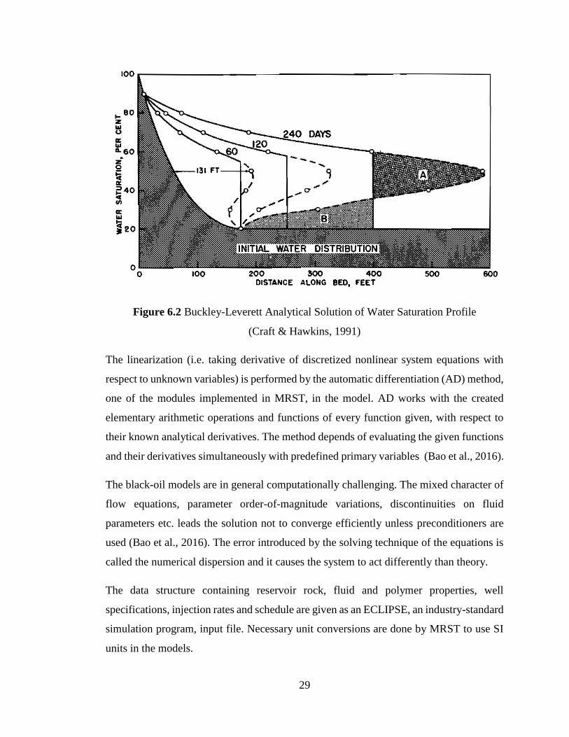
However, discontinuity in the saturation function causes the result of equation 6.13 to give
two saturation values for each position. A disconitnuity at the water front position is
defined and areas below that position are balanced and the corrected water saturation
profile can be obtained. Figure 6.2 shows an illusturation of the correction done on the
analytical solution at different time steps by Craft & Hawkins (1991).
6.3 Polymer Model of MRST
MRST solves the grid system and continuity equations given in Chapter 5 with respect to
grid, reservoir, and polymer information defined in the input file by implicit discretization
of the governing equations. Discrete continuous divergence and gradient operators are
defined, and flow equations are discretized in very compact form. Implicit temporal
discretization and standard two-point spatial discretization are used for conservation
equations. The continuity equations, well rates, and well control equations are collected
in a problem system. The nonlinear system of equations is solved using the Newton’s
method, and multidimensional Taylor expansions are used to derive the iterations.
29
Figure 6.2 Buckley-Leverett Analytical Solution of Water Saturation Profile
(Craft & Hawkins, 1991)
The linearization (i.e. taking derivative of discretized nonlinear system equations with
respect to unknown variables) is performed by the automatic differentiation (AD) method,
one of the modules implemented in MRST, in the model. AD works with the created
elementary arithmetic operations and functions of every function given, with respect to
their known analytical derivatives. The method depends of evaluating the given functions
and their derivatives simultaneously with predefined primary variables (Bao et al., 2016).
The black-oil models are in general computationally challenging. The mixed character of
flow equations, parameter order-of-magnitude variations, discontinuities on fluid
parameters etc. leads the solution not to converge efficiently unless preconditioners are
used (Bao et al., 2016). The error introduced by the solving technique of the equations is
called the numerical dispersion and it causes the system to act differently than theory.
The data structure containing reservoir rock, fluid and polymer properties, well
specifications, injection rates and schedule are given as an ECLIPSE, an industry-standard
simulation program, input file. Necessary unit conversions are done by MRST to use SI
units in the models.

30

31
CHAPTER 7
7PARTICLE MODEL
Random-walk particle tracking model is explained in this chapter.
7.1 Random Walk Particle Model Description
Kinzelbach (1990) states in his work that the random walk method comes from statistical
physics, which is used to solve diffusion and dispersion problems in porous medium. The
main advantage of the method is that it does not show numerical dispersion in the solution.
The transport equations in porous media are the second order initial value problem type
partial differential equations. Their results are unreliable because of the combination of
hyperbolic advection equation and parabolic diffusion/dispersion equation unless strict
preconditioners are used. Random walk method is simple, can be added on any flow
model, and matches with the analytical solution at comparable computational effort.
However, due to its random nature, the method gives randomly fluctuated concentration
profiles. Size of the fluctuations can be reduced by increasing the number of particles used
in the simulations. Still, increased number of particles does not improve the result at the
same rate because the statistical uncertainty is proportional to the inverse square root of
the count of particles in a cell.
The method starts with the injection of the known-mass particles representing polymer
mass/concentration in the water phase into the system at a uniform velocity. The positions
of the particles are updated with the combinations of the effects of advection and diffusion.

32
Meaning that the particles moves with the water velocity of the cell for the time step and
diffuses/disperses into the system. As discussed in Chapter 3, diffusion can be analyzed
statistically and with normal distribution. Equation 3.14 is the distance travelled by 68%
of the chemical injected. Cranmer, 2003 gives the probable distance travelled by a particle
as:
∆𝑥𝑠𝑝𝑟𝑒𝑎𝑑 = 𝒩(𝜉)√2𝐷0Δ𝑡 (7.1)
where, 𝒩(𝜉) is a sample from a normal distribution with zero mean and unit variance.
𝒩(𝜉) =1
√2𝜋𝑒−𝜉2/2
(7.2)
Movement of the particle in the model can be shown schematically as in Figure 7.1.
Figure 7.1 Particle Movement Represantation (Prickett, Naymik, & Lonnquist, 1981)
Positions of the particles are updated as:
𝑥𝑖𝑛+1 = 𝑥𝑖
𝑛 + 𝜐𝑤𝑛 ∆𝑡 + ∆𝑥𝑠𝑝𝑟𝑒𝑎𝑑 (7.3)
where 𝑥𝑖 is the position of particle and superscript n denotes the time step. The terms after
the old position of the particle are the advection and spreading terms respectively.
33
Concentration profile can be obtained by counting the particles in each grid cell and
dividing the mobile mass of particles to the water volume at the corresponding cell. The
concentration distribution is fluctuated due to the randomness of the process as discussed
before. There should be at least 20 particles in a cell to calculate the concentration
properly. Duration of 5 to 10 time steps for a particle to leave a grid cell also helps the
results to be smoother (Kinzelbach, 1990).
7.2 Assumptions in the Model
In constructing the model during this study, some assumptions are made. In the model, it
is assumed that the polymer only is present in water phase like MRST model does.
Particles have the velocity of water in the porous medium. Advection of particles is carried
out by the water velocity in each cell at the corresponding time step.
The spreading distance of the particles at each time step, ∆𝑡, due to diffusion and
dispersion is calculated by taking the spreading length as 𝒩(𝜉)√2𝐷𝐶∆𝑡. The dispersion
coefficient, 𝐷𝐶, used in the calculations involves effects of both diffusion and dispersion.
Sheng (2011) states the typical diffusion coefficient as 4 x 10⁻¹⁰ m2/s in the porous
medium. This value is multiplied by the dispersivity of the reservoir using Equation 3.18
to find the dispersion coefficient, 𝐷𝐶 in the model. Length term used in Equation 3.18 is
the total length of reservoir in the problem. A normally distributed scalar, with mean of 0
and standard deviation of 1, at each time step for each particle is randomly generated to
obtain 𝒩(𝜉).
7.3 Movement of the Particles
Particles are injected with water at a constant rate and concentration in the problems. By
using these information, mass of each particle is obtained and they are positioned in the
center of the injection well at t = 0. Then a predetermined number of particles with
calculated initial mass are released and then advected and dispersed at each time step along
with the currently present particles in the system, and their mass is updated by adsorption
process.

34
In the 1D problem, the movement occurs only in one direction, therefore advection and
dispersion is modelled with ease. However, in the 2D scenarios, velocity vectors consists
of x and y components at cell centers as averages. The releasing of particles should be in
radial form. This condition is provided by assigning a uniformly distributed angle to each
particle at the injection point. At the injection cell, instead of using the velocity field value
for injection velocity, velocity calculated from the injection flow rate and wellbore cross
sectional area is used. Newly released particles follow the same angle while in the
injection cell. If a particle leaves the no-flow boundary, it is repositioned into the grid
system by the distance it travelled outside of it in the same direction. By doing so, we
prevent the system from giving errors because of misplaced particles.
MRST solution provides the x and y components of the velocity vector field at cell centers
as averages. In order to provide more realistic velocity values for particles, the interpolated
velocity at their exact location in the grid system is used for advection. This approach is
better in 2D problems, because it provides a better distribution pattern.
Concentration in each cell is calculated as described in Chapter 8.1 at each time step as:
𝑐 =𝑚𝑝
𝑉Φ𝑆𝑤
(8.4)
where:
𝑚𝑝 = Mobile polymer mass in the cell, kg
𝑉 = Volume of the cell, m3
This concentration information is used to calculate the amount of polymer to be adsorbed
to the rock surface. Concentration of polymer and corresponding polymer mass that can
be adsorbed by unit mass of rock is given as a table by the user to the system.
𝑚𝑎𝑑𝑠𝑛 = ℳ𝜌𝑟𝑉(1 − Φ(1 − 𝑆𝑑𝑝𝑣)) (8.5)
where:
𝑚𝑎𝑑𝑠𝑛 = Mass of polymer that can be adsorbed by the cell at the current time step, kg

35
ℳ = Mass of polymer that can be adsorbed by unit mass of rock, kg
If 𝑚𝑎𝑑𝑠𝑛 is greater than 𝑚𝑎𝑑𝑠
𝑛−1, which is the already adsorbed polymer mass at the previous
time steps, the difference between 𝑚𝑎𝑑𝑠𝑛 and 𝑚𝑎𝑑𝑠
𝑛−1 is taken to be the adsorbed at the
current time step. Then, mass of each particle in the cell is reduced equally to add the
adsorption effect.
𝑚𝑟𝑒𝑑 =𝑚𝑎𝑑𝑠
𝑛 − 𝑚𝑎𝑑𝑠𝑛−1
𝒩
(8.6)
where 𝑚𝑟𝑒𝑑 is the mass to be reduced from each particle, and 𝒩 is the number of particles
present in the cell.
The particles that reaches the production well during the simulation are reduced to zero
mass and positioned at the production well location to ignore their effects on the process.

36

37
CHAPTER 8
8STATEMENT OF PROBLEM
The aim of this study is to use random walk particle tracking method with MRST to model
polymer injection. Discretization of the continuity equations solved in black-oil simulators
by numerical methods involves an error, which is called numerical dispersion. Numerical
dispersion causes the system to act differently than theory. The particle tracking method
is used to overcome the effects of numerical dispersion on polymer distribution. The
continuity equation for the polymer phase is solved by introducing particles representing
a known mass of polymer. Effects of polymer injection in the system is included by
calculating the concentration field, from particles’ position and mass information. The
method uses water phase velocity obtained from MRST to introduce advection on the
particles. Dispersion of the particles is modelled by assigning a dispersivity coefficient
and random walk method. Polymer adsorption on rock surface is added by updating
particle masses with respect to concentration and adsorption capacity of rock. The
polymer concentration field calculated by MRST is updated with the concentration field
from the particle tracking method at each time step. MRST then utilizes the field in
calculation of flow characteristics of the oil and water phases.

38

39
CHAPTER 9
9RESULTS & DISCUSSION
9.1 Verification of MRST Models
Before implementing the random walk particle tracking method into MRST, a verification
study on MRST solutions has been carried out as stated in Chapter 6.
9.1.1 Buckley-Leverett Verification
For verification of MRST solvers, a basic 1D problem with 100 grids is created and solved
with both MRST and Buckley-Leverett analytical solution. Reservoir and fluid properties
of the problem are obtained from Willhite (1986) and stated below:
The reservoir is 300 ft wide, 20 ft thick, and 1000 ft long
Φ = 0.15
Swc = 0.363, Sor = 0.205
Sw = 0.363, So = 0.637
Injection well is located in one end of the reservoir and qt = 53.7 m3/day
μw = 1.0 cp, μo = 2.0 cp
𝑘𝑜 = (1 − 𝑆𝑤𝐷)2.56
𝑘𝑤 = 0.78𝑆𝑤𝐷3.72
𝑆𝑤𝐷 =𝑆𝑤−𝑆𝑤𝑐
1−𝑆𝑜𝑟−𝑆𝑤𝑐

40
Corresponding relative permeability and fractional water flow curves are obtained in
MATLAB and given below in Figures 9.1 and 9.2.
Figure 9.1 Relative Permeability Curve
Figure 9.2 Fractional Flow & Derivative

41
The problem is solved with no flow boundary conditions and incompressible transport,
using block system of linear equations of interface fluxes and cell pressures at the next
time step. Water saturation profile of the MRST solution is compared with the flood front
position gathered from Equation 6.13 throughout 400 days of injection. Gathered profiles
can be seen on Figure 9.3.
Figure 9.3 Comparison of Flood Front Position (a) t = 100 days (b) t = 200 days

42
Figure 9.3 (cont’d) Comparison of Flood Front Position (c) t = 400 days
The movement of flood front of both analytical and MRST solutions are coherent with
each other.
9.1.2 ECLIPSE Verification
ECLIPSE is a simulator developed by the company Schlumberger having various
modelling options and methods used in the industry. ECLIPSE 100, the black-oil
simulator, is used in this study to compare the consistency of polymer model of MRST. A
fully implicit model is used in the system to treat oil/water/gas/polymer/brine system
(Schlumberger, 2015).
For the sake of verification, dataset downloaded from MRST polymer tutorial website
(Sintef, n.d.-b) is modified to be a one dimensional continuous polymer injection problem.
The dataset is run on ECLIPSE and concentration profile is obtained from each grid cell
in the model. Concentration profile from both MRST and ECLIPSE solutions plotted
together against distance to injection well to see their match in MATLAB at different
times of the injection. Plotted results can be seen on Figure 9.4.
Figure 9.4 shows that the concentration profile obtained from MRST solution matches
with ECLIPSE solution.

43
Figure 9.4 Comparison of Polymer Concentration Profiles (a) t = 200 days (b) t = 600
days (c) t = 1000 days
44
9.2 Numerical Dispersion
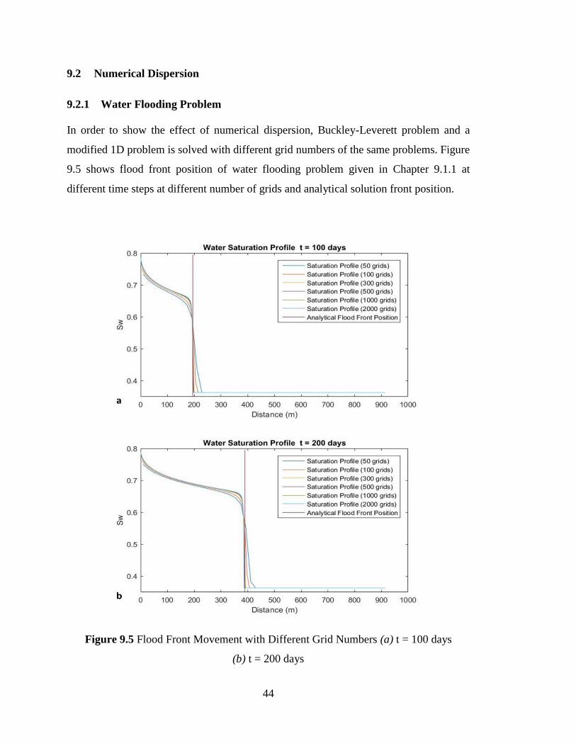
9.2.1 Water Flooding Problem
In order to show the effect of numerical dispersion, Buckley-Leverett problem and a
modified 1D problem is solved with different grid numbers of the same problems. Figure
9.5 shows flood front position of water flooding problem given in Chapter 9.1.1 at
different time steps at different number of grids and analytical solution front position.
Figure 9.5 Flood Front Movement with Different Grid Numbers (a) t = 100 days
(b) t = 200 days

45
Figure 9.5 (cont’d) Flood Front Movement with Different Grid Numbers
(c) t = 400 days
All obtained saturation profiles from different number of grid systems of the same
problem shows a curvature at the front position. The curvature observed is the result of
numerical dispersion and the rate of divergence from the theoretical front position does
not improve much after 300 grids. The effect of numerical dispersion is always present in
the numerical solution.
9.2.2 1D Polymer Injection Problem
In all of our problems, a modified MRST polymer tutorial dataset obtained from MRST
website (Sintef, n.d.-b) is used to create and solve an oil/water/polymer problem. All
polymer injection scenarios use complete mixing of polymer with water. The effect of
polymer on water viscosity and adsorption capacity of the rock are given as tables in the
input file, and are not modified. Corresponding plots of viscosity multiplier and adsorption
curve can be seen on Figure 9.6 and 9.7 respectively. Polymer adsorption process in the
reservoir is taken irreversible.

46
Figure 9.6 Viscosity Multiplier
Figure 9.7 Polymer Adsorption Curve
In our 1D polymer injection scenario, injection well is positioned in the first grid cell and
production well is at the last grid cell of the system. Rest of the important properties are
given in the Table 9.1.

47
Table 9.1 One Dimensional Problem Properties
Property Value
Total Dimensions (x-y-z) 200 m – 20 m – 4 m
Porosity 30 %
Permeability 100 mD
𝑺𝒅𝒑𝒗 5 %
RRF 1.1
𝝆𝒓𝒐𝒄𝒌 2000 kg/m3
Water Injection Flow Rate 10 m3/day
Injected Polymer Concentration 0.8 kg/m3
∆𝒕 0.5 days
Total Simulation Time 500 days
In order to observe the effect of numerical dispersion, the problem given above is solved
with different number of grids. Figure 9.8 shows polymer concentration profile movement
plotted at two different time steps.
Figure 9.8 Polymer Concentration Profile with Different Grid Numbers (a) t = 100 days

48
Figure 9.8 (cont’d) Polymer Concentration Profile with Different Grid Numbers
(b) t = 200 days
Figure 9.8 shows the effect of numerical dispersion decreases with increasing number of
grids in the system. However, it is not completely removed and the computation time
increase with increasing number of grids also. The numerical dispersion is not smoothed
much after 400 grids representation of the 1D problem. Therefore, 400 grids are used for
this problem in the rest of the study. The numerical dispersion effect can also be smoothed
with shorter time steps, since it leads to better representation of flow process. However,
the numerical solution would still cause numerical dispersion in the results.
9.3 Implementation of Model into MRST
Idea behind the implementation of the random walk particle tracking method into MRST
is initializing and moving the particles, then updating the concentration profile that MRST
calculates by our profile at each time step. MRST solves all the equations given in Chapter
5 at each time step, including polymer phase. Our model solves the particle system
simultaneously with MRST at each time step by using water phase velocity calculated
from MRST. Interpolated water phase velocity field is used for particles’ exact positions
in the problems. Effect of interpolation is better seen on 2D problems, therefore will be
explained later. Working principle of particle model with MRST is summarized in the
flow chart seen on Figure 9.9 at each time step.

49
Figure 9.9 Solution Flow Chart
By updating concentration field information of MRST solution at the end of each time
step, we aim to eliminate the effects of polymer continuity equations.
In each scenario, 100 particles per time step is used. However, only 20 particles per each
time step is plotted in order to visualize the particles with ease and reduce computation
time. Time step length and total time required are arranged to see the effect of polymer
after it reaches to production wells.
9.4 1D Problem
In our 1D polymer injection scenario, problem set described in Chapter 9.2.2 is used with
400 grids. First, we checked the polymer concentration obtained from the MRST solution,
in order to see the model behavior. In Figure 9.10, polymer concentration and saturation
movement throughout the reservoir can be seen at different time steps.
Two saturation front occurs as expected and stated in Pope, 1980 throughout the injection
process. The first front is the result of increasing saturation velocity in the upstream as in
a waterflooding application. The following saturation front occurs at the polymer
concentration front, which is the connection point of polymer water and connate water of
the system. This trend can be seen on Figure 9.10 also.

Figure 9.10 MRST Polymer Concentration & Saturation Profiles (a) t = 100 days (b) t = 300 days
50

51
Figure 9.10 (cont’d) MRST Polymer Concentration & Saturation Profiles
(c) t = 500 days
Then our profile is replaced with MRST at each time step and profiles are plotted. Figure
9.11 shows the concentration and saturation movement at different time steps. Saturation
profiles of both of the solutions can be seen in the Figure 9.11 also.

Figure 9.11 Particle Polymer Concentration & Saturation Profiles (a) t = 100 days (b) t = 300 days
52

53
Figure 9.11 (cont’d) Polymer Concentration & Saturation Profiles (c) t = 500 days
Most of the particles that falls ahead of the concentration front has lost their mass to
reservoir rock due to adsorption. Those particles are not counted in particle concentration
calculation and not plotted in Figure 9.11. The random nature of the particles can be seen
as fluctuations in the profile but it seems to agree with injection concentration in the
reservoir. Effect of the fluctuations can also be seen on both saturation profiles in Figure
9.11. Production curves are obtained at the end of injection and in Figure 9.12, comparison
of MRST and Particle production curves of four different realizations, in other words, four
different possibilities of the solution, is plotted. The effect of random movement can also
be seen on Figure 9.12 after polymer reaches the production well in the reservoir.

Figure 9.12 1D Production Curve Comparisons
54

55
Particle method concentration front is more piston like and falls behind the MRST
concentration profile in time in Figure 9.11. Numerical dispersion causes MRST profile
to move faster and polymer to reach earlier to the production well. This effect and the
piston like movement of the saturation profiles can also be seen in Figure 9.11 in particle
method profiles as it follows the concentration front. The effect of numerical dispersion
can be clearly seen on both figures 9.11 and 9.12. MRST profile reaches earlier and shows
a curved nature instead of a steep change.
9.4.1 Effect of Dispersion Coefficient
If the flow is advection dominant in the reservoir, movement of flood fronts and shape of
production curve should be more piston like. If reservoir has high heterogeneities, the flow
can be dispersion dominant. The dispersion is not taken into account in continuity
equations solved in the system normally. The dispersion effect only comes numerically.
This effect can be modelled by changing the dispersion coefficient used in particle
method. In order to see the effect of dispersion coefficient on polymer application,
Equation 3.18 is changed in other realizations. Figure 9.13 shows the effect of dispersion
coefficient changes on concentration profile movement at 200th day of injection.
Figure 9.13 Effect of Dispersivity Coefficient on Polymer Concentration Movement
The effect of dispersion coefficient on production curves is also plotted on Figure 9.14.

Figure 9.14 Effect of Dispersivity Coefficient (a) Dc x 0.1 (b) Dc x 1 (c) Dc x 10 (d) Dc x 50
56

Figure 9.14 (cont’d) Effect of Dispersivity Coefficient (e) Dc x 100 (f) Dc x 200 (g) Dc x 300 (h) Dc x 500
57

58
Figures 9.13 and 9.14 shows that when we increase the dispersion coefficient used in the
model, it converges more to the MRST solution. However, the uncertainties also increase
with the increased dispersion coefficient.
9.4.2 Effect of Particle Number Injected
Number of particles injected to the system defines the number of particles to be present in
a grid during the simulation. With increased number of particles, particle masses that
represent polymer mass injected are reduced. If low number of particles are used, we
should see more uncertainties in terms of concentration calculation. The same 1D problem
is solved with four different total particle number injected throughout the simulation to
see its effect on calculations. In four different simulations of the same problem, 10, 50,
100, and 200 particles per time step are injected respectively. Figure 9.15 shows the
concentration profile movement at 200th time step of simulation and the concentration
profile obtained from MRST solution only, without visualizing the particle positions.
Figure 9.15 Polymer Concentration Profile with Different Number of Particles
(a) 10000 particles

59
Figure 9.15 (cont’d) Polymer Concentration Profile with Different Number of Particles
(b) 50000 particles (c) 100000 particles (d) 200000 particles

60
The uncertainties on concentration calculation causes the solution not to give good
production results of simulation with low number of particles injected. After 100 particles
per time step injected, the results does not change much.
9.5 2D Problem
9.5.1 Velocity Field Interpolation
MRST provides the components of the velocity vector field, as stated in Chapter 7.3.
Direct use of the vectors for advection therefore causes the particles to move along the
resultant velocity vector after they leave the injection cell. Instead of using the velocity
vectors directly, they are interpolated in grid cells with respect to particle position for each
particle to provide a proper advection path. Interpolated velocity field is used in both 1D
and 2D problems but its effects are more obvious in 2D problems. In order to visualize
the effect of interpolation on the velocity field, an example constant velocity field is
obtained and used to inject particles in a grid system of 30 m x 30 m. Figure 9.16 shows
the velocity vectors and movement of particles in a short time period, and the need for
interpolation to provide a proper distribution.
Figure 9.16 Effect of Velocity Field Interpolation on Particle Distribution,
without Interpolation (a), with Interpolation (b)

61
9.5.2 1st Scenario
In our 2D problem, 1D problem dataset is updated to have equal dimension grid blocks
and a square reservoir representation. Our 1st scenario includes one injection well on the
lower left grid, and one production well on the upper right grid of the system. Rest of the
properties of the scenario can be seen on Table 9.2. Particles are released into the system
with as explained in Chapter 7.3.
Table 9.2 Two Dimensional Problem 1st Scenario Properties
Property Value
Grids (x – y – z) 30 – 30 – 1
Total Dimensions (x – y – z) 180 m – 180 m – 2 m
Porosity 30 %
Permeability 100 mD
𝑺𝒅𝒑𝒗 5 %
RRF 1.1
𝝆𝒓𝒐𝒄𝒌 2000 kg/m3
Water Injection Flow Rate 10 m3/day
Injected Polymer Concentration 0.8 kg/m3
∆𝒕 1 days
Total Simulation Time 1400 days
Polymer concentration profiles can be plotted as a color map in this scenario. Figure 9.17
shows the MRST and particle concentration profiles at different time steps. In Figure 9.18,
distribution of particles can be seen areally. Obtained production results of four different
realizations is again plotted and shown in Figure 9.19.
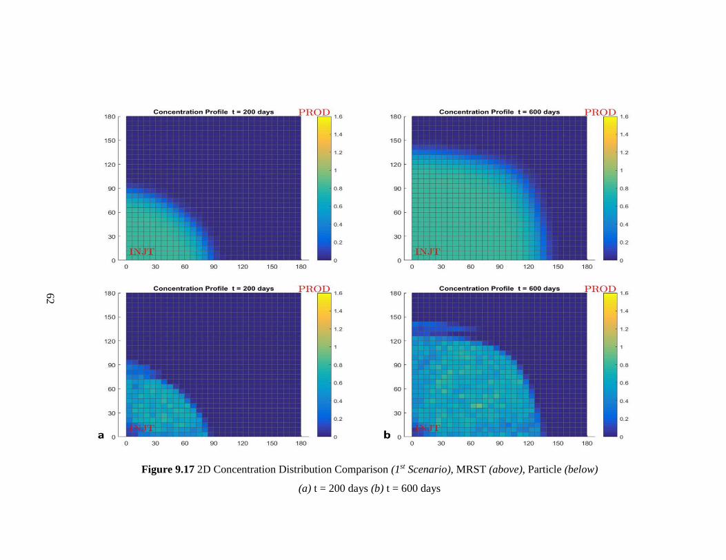
Figure 9.17 2D Concentration Distribution Comparison (1st Scenario), MRST (above), Particle (below)
(a) t = 200 days (b) t = 600 days
62

Figure 9.17 (cont’d) 2D Concentration Distribution Comparison (1st Scenario), MRST (above), Particle (below)
(c) t = 1000 days (d) t = 1400 days
63
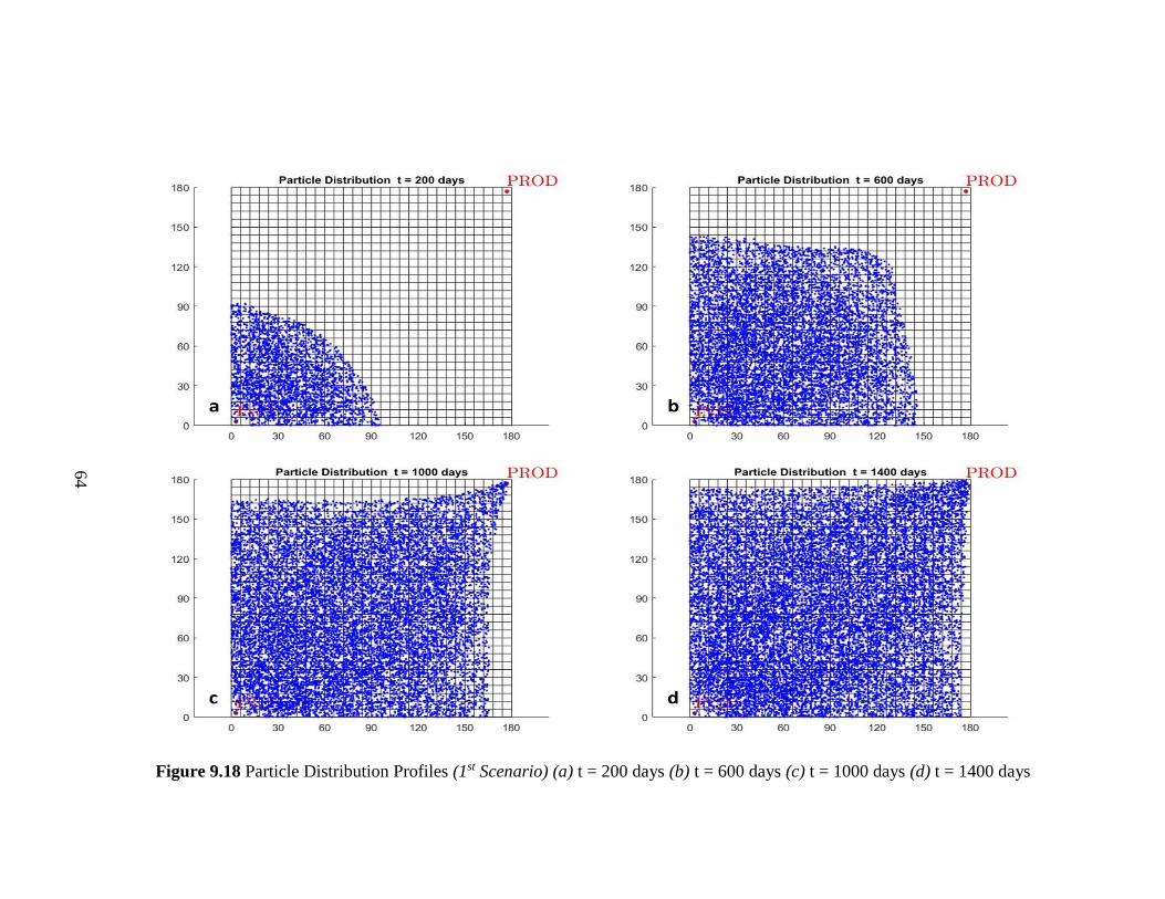
Figure 9.18 Particle Distribution Profiles (1st Scenario) (a) t = 200 days (b) t = 600 days (c) t = 1000 days (d) t = 1400 days
64

Figure 9.19 2D Production Curve Comparison (1st Scenario)
65

66
4th realization of this scenario gave a different production curve than the rest of the runs.
Randomly generated angles used for injection and random numbers used on dispersion of
the particles can lead the particles to accumulate in some regions of the system. The effect
of accumulation affects the system and different results can be seen in some simulations.
However, the other results seems to agree with each other and the effect of numerical
dispersion is not seen on the results.
9.5.3 2nd Scenario
In our 2nd scenario, the dataset is updated to have one production well on the lower left
and one on the upper right grid of the system, and one injection well at the center grid.
Particle releasing on the system is the same and the rest of the properties of the scenario
can be seen on Table 9.3.
Table 9.3 Two Dimensional Problem 2nd Scenario Properties
Property Value
Grids (x – y – z) 30 – 30 – 1
Total Dimensions (x – y – z) 180 m – 180 m – 2 m
Porosity 30 %
Permeability 100 mD
𝑺𝒅𝒑𝒗 5 %
RRF 1.1
𝝆𝒓𝒐𝒄𝒌 2000 kg/m3
Water Injection Flow Rate 10 m3/day
Injected Polymer Concentration 0.8 kg/m3
∆𝒕 1 days
Total Simulation Time 1000 days
Figure 9.20 shows the concentration distribution at different time steps of the injection.
Figure 9.21 shows the particle distributions. Comparison of MRST and Particle
production curves are plotted on Figure 9.22.

Figure 9.20 2D Concentration Distribution Comparison (2nd Scenario), MRST (above), Particle (below)
(a) t = 100 days (b) t = 400 days
67
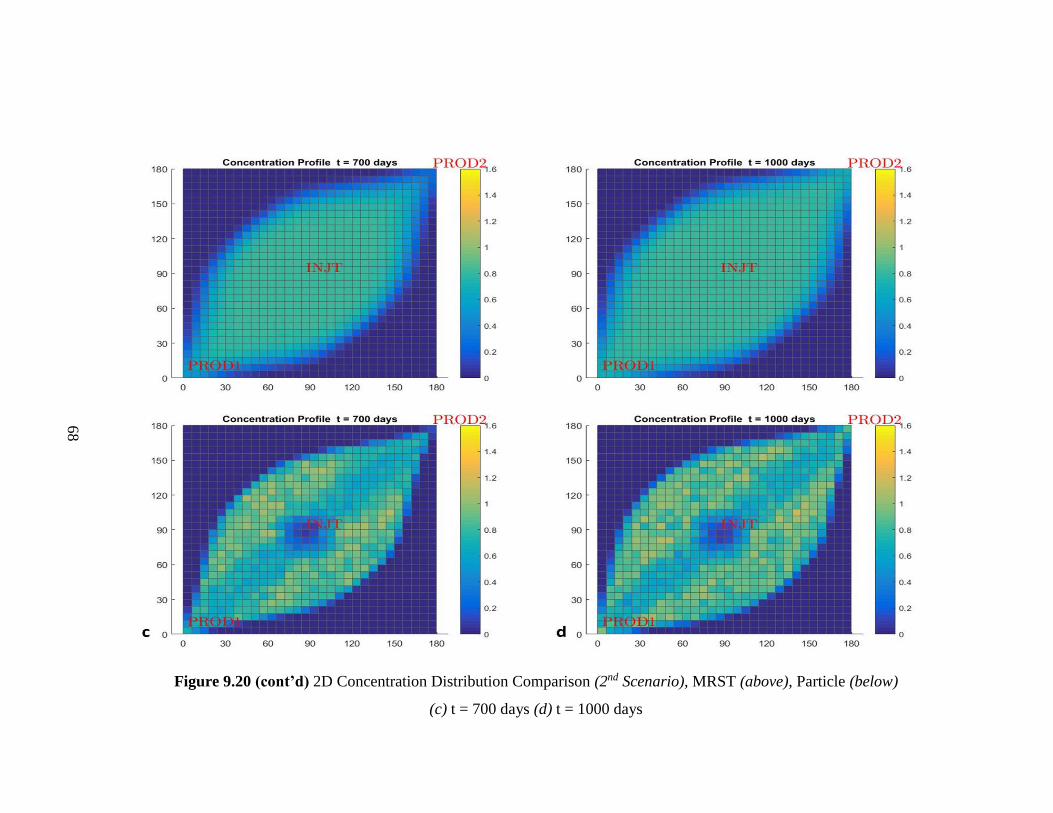
Figure 9.20 (cont’d) 2D Concentration Distribution Comparison (2nd Scenario), MRST (above), Particle (below)
(c) t = 700 days (d) t = 1000 days
68

Figure 9.21 Particle Distribution Profiles (2nd Scenario) (a) t = 100 days (b) t = 400 days (c) t = 700 days (d) t = 1000 day
69

Figure 9.22 2D Production Curve Comparison (2nd Scenario)
70

71
Since there are two production wells at this scenario, the production curve is the
summation of both of the wells. The physical effect of dispersion is seen less and the
results vary more than the other scenarios, but still the overall profiles agree with MRST
solution. In some runs, the problem did not converge because of high accumulation of
particles at some cells. Generated random numbers, effect of polymer on velocity fields,
and overall velocity field generated by the MRST might cause the high accumulation in
this problem.

72

73
CHAPTER 10
10CONCLUSION
Random-walk particle tracking method gives an alternative modelling option for polymer
flooding. The technique is used to solve polymer advection and diffusion/dispersion
equation to add the effects of injected polymer to a reservoir. MRST model solves the set
of equations for the system. Simultaneously polymer concentration profile is calculated
with the updated position and mass information of particles’ at each time step. The effects
of polymer on other properties in the reservoir and flow are dependent on polymer
concentration in the reservoir. In order to eliminate the equations solved for polymer phase
in the MRST model, concentration profile calculated by MRST model is updated with the
profile calculated from the polymer concentration at each time step.
MRST model does not include the dispersion process. Effect of dispersion occurs
numerically on MRST model solutions of simple water flooding and 1D problem even
though finer grid systems are used to overcome the effect. Particle tracking method allows
us to define a dispersion parameter that is used to calculate the transport of polymer
probabilistically. Since the transportation of polymer is calculated with a linear equation,
it does not involve numerical errors. Dispersion coefficient used can be changed easily in
the model. A high dispersivity reservoir shows similar results with MRST solution. The
model can be used to determine the dispersivity of a reservoir with field data in simple 1D
problems.

74
Oscillations in the concentration calculations are the result of the random nature of the
problem. They can be lowered with higher particle numbers released into the system. If
small numbers of particles or long time steps are applied, the number of particles in a cell
leads to more oscillations and uncertainties in the calculations. Increasing the number of
particles injected does not improve much after some point, but it also increases the
computation time of the model.
In 2D scenarios, particle solution shows a general consistency with some exceptions.
Generated random numbers used in injection modelling can cause the particles to
accumulate in an area with the combined effect of water velocity profiles obtained from
MRST solution. This effect is seen on the production curve generated in our 1st scenario,
whereas in the 2nd scenario, the problem might not converge to a solution at some
simulations.
As a result, random-walk particle tracking method can be a tool to overcome the effect of
numerical dispersion in simple 1D models, whereas it can still be an alternative in 2D
scenarios in polymer injection modelling.
For future works, reservoir heterogeneities, different grid orientations, effect of salinity
can be worked with the model. In addition to different reservoir and chemical systems,
some smoothing methods can be introduced to the model in order to reduce the oscillations
in the calculations.
75
11REFERENCES
Arya, A., Hewett, T. A., Larson, R. G., & Lake, L. W. (1988). Dispersion and Reservoir
Heterogeneity. SPE Reservoir Engineering, 3(1), 139–148.
https://doi.org/10.2118/14364-PA
Bao, K., Lie, K. A., Møyner, O., Liu, M., Neidinger, R. D., Xin, J., & Odeh, A. (2016).
Fully implicit simulation of polymer flooding with MRST. 15th European
Conference on the Mathematics of Oil Recovery, ECMOR 2016, 42(3), 545–563.
https://doi.org/10.3997/2214-4609.201601880
CMG. (2010). Advanced Process and Thermal Reservoir Simulator. Calgary, Alberta
Canada: Computer Modelling Group Ltd.
Craft, B. C., & Hawkins, M. (1991). Applied Petroleum Reservoir Engineering.
Cranmer, S. R. (2003). Monte Carlo Solutions to Diffusion-Like Equations : A Practical
Application of the Ito Calculus. Harvard-Smithsonian Center for Astrophysics,
Cambridge, (2).
Dake, L. P. (1998). Fundamentals of Reservoir Engineering. Amsterdam, London, New
York, Tokyo: Elsevier.
Dandekar, A. Y. (2013). Petroleum Reservoir Rock and Fluid Properties, Second Edition
(Second Edi). Boca Raton, London, New York: CRC Press.
Donaldson, E. C., Chilingarian, G. V., & Yen, T. F. (Eds.). (1989). Enhanced Oil
Recovery, II Processes and Operations. Developments in Petroleum Science (Vol.
17). Amsterdam, London, New York, Tokyo: Elsevier.
Ertekin, T., Abou-Kassem, J. H., & King, G. R. (2001). Basic Applied Reservoir
Simulation. Richardson, Texas: SPE.
Gogarty, W. B. (1967). Mobility Control With Polymer Solutions. SPE Journal, 161–173.
https://doi.org/10.2118/1566-B
Green, D. W., & Willhite, G. P. (1998). Enhanced Oil Recovery. Richardson, Texas: SPE.
76
Inoue, K., Takao, Y., & Tanaka, T. (2009). Application of Random Walk Particle
Tracking to the Delineation of Capture Zones. In International Offshore and Polar
Engineering Conference (Vol. 1, pp. 311–317).
John, A. K., Lake, L. W., Bryant, S. L., & Jennings, J. W. (2010). Investigation of Mixing
in Field-Scale Miscible Displacements Using Particle-Tracking Simulations of
Tracer Floods With Flow Reversal. Spe Journal, 15(3), 598–609.
Kinzelbach, W. (1990). Simulation of Pollutant Transport in Groundwater with the
Random Walk Method. In Dresden Symposium (pp. 265–279).
Lacerda, E. C. M. S., Priimenko, V. I., & Pires, a P. (2012). Microbial EOR: A
Quantitative Prediction of Recovery Factor. Eighteenth SPE Improved Oil Recovery
Symposium, 1–10. https://doi.org/10.2118/153866-MS
Liu, H. H., Bodvarsson, G. S., & Pan, L. (2000). Determination of particle transfer in
random walk particle methods for fractured porous media. Water Resources
Research, 36(3), 707–713. https://doi.org/10.1029/1999WR900323
Mungan, N., Smith, F. W., & Thompson, J. L. (1966). Some aspects of Polymer Floods.
Journal of Petroleum Technology, (September), 1144–1150.
https://doi.org/10.2118/1628-PA
Özdemir, R. T. (2015). Particle Tracking Modeling of Marine Sediment Pollution. Middle
East Technical University.
Perkins, T. K., & Johnston, O. C. (1963). A Review of Diffusion and Dispersion in Porous
Media. Society of Petroleum Engineers Journal, 3(1), 70–84.
https://doi.org/10.2118/480-PA
Pope, G. a. (1980). The Application of Fractional Flow Theory to Enhanced Oil Recovery.
Society of Petroleum Engineers Journal, 20(3), 191–205.
https://doi.org/10.2118/7660-PA
Prickett, T. a, Naymik, T. G., & Lonnquist, C. G. (1981). A “Random-Walk” Solute
Transport Model for Selected Groundwater Quality Evaluations. Rep I 11 (Vol. 65).
Champaign: Illinois State Water Survery.
77
Rodriguez, S., Romero, C., Sargenti, M. L., Müller, a. J., Sáez, a. E., & Odell, J. a. (1993).
Flow of polymer solutions through porous media. Journal of Non-Newtonian Fluid
Mechanics, 49(1), 63–85. https://doi.org/10.1016/0377-0257(93)85023-4
Schlumberger. (2015). ECLIPSE Technical Description. Schlumberger.
Sheng, J. (2011). Modern chemical enhanced oil recovery : theory and practice. Gulf
Professional Pub.
Sintef. (n.d.-a). MRST - MATLAB Reservoir Simulation Toolbox. Retrieved July 13,
2017, from http://www.sintef.no/projectweb/mrst/
Sintef. (n.d.-b). MRST - MATLAB Reservoir Simulation Toolbox Polymer Tutorial.
Retrieved September 20, 2015, from
https://www.sintef.no/projectweb/mrst/publications/tutorials/tutorial_polymer/
Stalgorova, E., & Babadagli, T. (2012). Field-scale modeling of tracer injection in
naturally fractured reservoirs using the random-walk particle-tracking simulation.
SPE Journal, 17(2), 580–592. https://doi.org/10.2118/144547-PA
Willhite, G. P. (1986). Waterflooding. Richardson, Texas: SPE.
Zheng, B. C., & Wang, P. P. (1999). A Modular Three - Dimensional Multispecies
Transport Model. Tuscaloosa, Alabama.

78

79
APPENDIX A
12CODE IMPLEMENTED
Appendix A gives implemented code in MRST model for particle tracking method for 1D
problem. Arrays model, schedule, and state are obtained from MRST solution.
Section below shows code for initialization of particle and input parameters:
dt = schedule.step.val; % time step information taken from model
nSteps = numel(dt); % number of time steps
% Injection input (hard-coded)
Ci = 0.8; % polymer injection concentration, kg/m3
qi = 10.0/86400; % water injection flow rate, m3/day
Simu = '1D';
% Set up random walk parameters
nPstep = 100; % particles to be injected per time step
nPtotal = nSteps * nPstep; % total particle number
nPnow = 0; % active particle count in the system
part.x = zeros(nPtotal,1); % particle distance information
part.i = zeros(nPtotal,1); % particle grid information
part.k = randperm(nPtotal); % random permutation; to locate the particle on y-axis
part.m = ones(nPtotal,1)*qi*Ci*dt(1)/nPstep; % particle mass, kg

80
Section below is used for updating the position information of particles to injection well
location.
Rest of the code given below is repeated in each time step. First part computes interpolated
velocity field and introduces advection and dispersion to active particles in the system.
Second part is used for releasing new particles to the system at the current time step
nc = model.G.cells.num; % total grid number of the system
partmassads = zeros(nc, 1); % adsorbed particle mass in each cell
partmassads1 = zeros(nc, 1); % adsorption capacity of the cell at the current time
step
mobmass = zeros(nc, 1); % mobile particle mass at the time step in each cell
massdiff = zeros(nc, 1); % mass to be adsorbed by rock in each cell
% Set dispersion parameters
diffC = 4.0e-10; % a typical diff. coeff., m^2/s
dispX = 0.044*model.G.nodes.coords(end,1)^1.13; % dispersivity multiplier
dispC = dispX * diffC * 1; % dispersion coefficient used
dispL = sqrt(2*dispC*dt(1)); % dispersion length
dx = model.inputdata.GRID.DX(1);
inji = cell2mat(model.inputdata.SCHEDULE.control.WELSPECS(end,3)); %
injection well position
part.x = ones(nPtotal,1)*((inji-1)*dx+dx/2); % reposition particles to injection point
% Compute interstial water phase velocities
fW = state.flux(:,1); % water phase flux given by MRST solution
sW = state.s(:,1); % water saturation given by MRST solution
poro = model.rock.poro; % porosity information
vW = bsxfun(@rdivide,faceFlux2cellVelocity(model.G, fW),poro.*sW); % water
phase velocity in each cell
Fx = griddedInterpolant(dist,vW(:,1),'cubic','cubic'); % interpolated velocity handle
Xq = part.x(1:nPnow); % positions of the active particles
xVq = Fx(Xq); % advection velocity for active particles
part.x(1:nPnow) = part.x(1:nPnow) + xVq.*dT; % advection of active particles
% Introduce dispersion
part.x(1:nPnow) = part.x(1:nPnow) + randn([nPnow 1])*dispL; % dispersion of
active particles

81
After moving the particles, positions are checked and polymer concentration is calculated
with code below
% Release new particles with average cell velocities of their position
vW(1,1) = vW(1,1)*2; % velocity is doubled in the first cell
dTpart = dT/nPstep; % mini time step for continious release of particle during time
step
for id = 1:nPstep
currentcell = 1; % current position of newly released particles
for t = 1:(nPstep + 1 - id) % loop to update position particle in case it leaves
injection cell
part.x(nPnow + id) = part.x(nPnow + id) + vW(currentcell,1)*dTpart; %
advection of newly released particle
part.x(nPnow + id) = part.x(nPnow + id) + randn()*sqrt(2*dispC*dTpart); %
dispersion of newly released particle
pos = floor(part.x(nPnow + id)/dx) + 1; % position of particle at the end of mini
time step
if pos > currentcell % position check
currentcell = pos;
end
end
end
% increase active particle count
nPnow = nPnow + nPstep;
% Check and correct the particle positions against the boundaries
partidx = part.x(1:nPnow)<0;
part.x(partidx) = 0;
% Correct produced particle location an masses
iprod = part.x(1:nPnow)>model.G.nodes.coords(end,1)-dx/2;
part.x(iprod) = model.G.nodes.coords(end,1)-dx/2;
part.m(iprod) = 0.0;
% Update particle grid information
part.i(1:nPnow) = floor(part.x(1:nPnow)/dx) + 1;
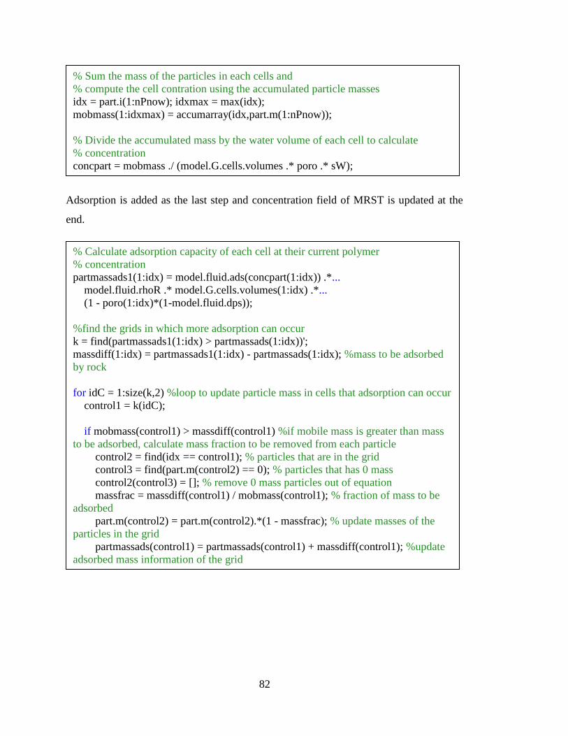
82
Adsorption is added as the last step and concentration field of MRST is updated at the
end.
% Sum the mass of the particles in each cells and
% compute the cell contration using the accumulated particle masses
idx = part.i(1:nPnow); idxmax = max(idx);
mobmass(1:idxmax) = accumarray(idx,part.m(1:nPnow));
% Divide the accumulated mass by the water volume of each cell to calculate
% concentration
concpart = mobmass ./ (model.G.cells.volumes .* poro .* sW);
% Calculate adsorption capacity of each cell at their current polymer
% concentration
partmassads1(1:idx) = model.fluid.ads(concpart(1:idx)) .*...
model.fluid.rhoR .* model.G.cells.volumes(1:idx) .*...
(1 - poro(1:idx)*(1-model.fluid.dps));
%find the grids in which more adsorption can occur
k = find(partmassads1(1:idx) > partmassads(1:idx))';
massdiff(1:idx) = partmassads1(1:idx) - partmassads(1:idx); %mass to be adsorbed
by rock
for idC = 1:size(k,2) %loop to update particle mass in cells that adsorption can occur
control1 = k(idC);
if mobmass(control1) > massdiff(control1) %if mobile mass is greater than mass
to be adsorbed, calculate mass fraction to be removed from each particle
control2 = find(idx == control1); % particles that are in the grid
control3 = find(part.m(control2) == 0); % particles that has 0 mass
control2(control3) = []; % remove 0 mass particles out of equation
massfrac = massdiff(control1) / mobmass(control1); % fraction of mass to be
adsorbed
part.m(control2) = part.m(control2).*(1 - massfrac); % update masses of the
particles in the grid
partmassads(control1) = partmassads(control1) + massdiff(control1); %update
adsorbed mass information of the grid

83
else %if mobile mass is less than mass to be adsorbed, reduce mass of each particle
in that grid to 0
control2 = find(idx == control1);
control3 = find(part.m(control2) == 0);
control2(control3) = [];
part.m(control2) = 0;
partmassads(control1) = partmassads(control1) + mobmass(control1); %update
adsorbed mass information of the grid
end
end
state.c = concpart; %update concentration array of MRST with particle method
concentration