rcee research in civil and environmental engineering · research in civil and environmental...
TRANSCRIPT
RCEE
Research in Civil and Environmental Engineering
www.jrcee.com
Research in Civil and Environmental Engineering 1 (2013) 79-91
NUMERICAL INVESTIGATION OF ANGLED BAFFLE ON THE FLOW
PATTERN IN A RECTANGULAR PRIMARY SEDIMENTATION TANK Elham Radaei a, Sahar Nikbinb, Mahdi Shahrokhi C*
a Master of Environmental Engineering, Amirkabir University of Technology, Tehran, Iran
b Master of Civil Engineering, Sharif University of Technology, Tehran, Iran
C*PhD of Civil Engineering, University Sains Malaysia, Nibong tebal , Penang, MALAYSIA
Keywords A B S T R A C T
Sedimentation tanks
Baffle Configuration
Numerical Modeling
VOF Method
ADV
It is essential to have a uniform and calm flow field for a settling tank with high performance. In general, however, the circulation zones always appear in the sedimentation tanks. The presence of these regions may have different effects. The non-uniformity of the velocity field, the short-circuiting at the surface and the motion of the jet at the bed of the tank that occurs because of the circulation in the sedimentation layer, are affected by the geometry of the tank. There are some ways to decrease the size of these dead zones, which would increase the performance. One is to use a suitable baffle configuration. In this study, the presence of baffle with different position and angle has been investigated by computational modeling. The results indicate that the best position and angle of the baffle is obtained when the volume of the recirculation region is minimized and the flow field trend to be uniform in the settling zone to dissipate the kinetic energy in the tank.
1 INTRODUCTION
Sedimentation is one of the most important units used in the treatment of industrial and domestic
wastewater. Although it is a conceptually simple process, it is actually complex in practice. There are two
main types of sedimentation tanks: primary and secondary. Primary settlers have a low influent
* Corresponding author (e-mail: [email protected]).
Elham Radaei et al - Research in Civil and Environmental Engineering 1 (2013) 79-91
80
concentration. Flow field in these tank are not influenced by concentration field, and the buoyancy effects
can be negligible. Secondary settlers have a higher influent concentration resulting in increased particle size
and the flow field being influenced by concentration distribution (Metcalf, 2003).
The sedimentation performance depends on the characteristics of the suspended solid and flow field in
the tank. Given that there is low concentration in the primary settling tanks, flow-field is not influenced by
particles; further, the flow pattern and the track taken by suspended solid through the tank are closely
linked to each other and the settling tank efficiency (Stamou et al., 1989). The flow field in the
sedimentation tanks is turbulent, and such turbulence affects particle concentration and deposition; thus, if
the turbulence is not predicted correctly, it may cause re-suspension of particles that have already settled.
Recent numerical models have shown fractional success in predicting the velocity field and the
concentration distribution of suspended solids in sedimentation tanks (Abdel-Gawad and McCorquodale,
1984; Celik et al., 1985; Imam et al., 1983; Larsen, 1977; Schamber and Larock, 1981). On the other hand,
several researchers have used the two-equation k-ε turbulence model (Celik et al., 1985; Schamber and
Larock, 1981).
Circulation zones are also called dead zones in sedimentation tanks because water is trapped and
particulate fluid has less volume for flow and deposition in these regions. Therefore, the existence of the
large circulation regions can lower tank performance. Circulation regions or dead zones in the settling tanks
create high flow mixing problems and cause the optimal particle sedimentation to decrease. Thus, the
important objective in designing settling tanks is to decrease the likelihood of the formation of the
circulation region. One applicable method to reduce the volume of the dead zones and increase the
performance of the sedimentation tanks is to use a proper baffle configuration (Razmi et al., 2009).
Bretscher et al. (1992) showed that intermediate baffle in a rectangular clarifier affected the velocity
and concentration fields. Goula et al. (2008) used a numerical model to study the particle settling in a
sedimentation tank using a vertical baffle installed in the inlet section; they showed that the baffle
increased the particle settling efficiency from 90.4% for a standard tank without baffle to 98.6% for one
with an installed baffle. Al-Sammarraee et al. (2009) concluded that the installation of baffles can improve
the efficiency of the tank in terms of settling. The baffles act as barriers that effectively suppress the
horizontal velocities of the flow and force the particles to the bottom of the basin.
In present work, the investigations of the baffle position and angle effects on the settling efficiency were
performed via some experiments and computational simulation. In experimental part of the work, a thin
baffle is positioned in a laboratory settling tank and the effects of its position on the velocity fields were
measured using Acoustic Doppler Velocimeter (ADV). Furthermore, results of the experimental part were
used for verification of the numerical modeling. Then, numerical experiments are performed for baffle
installation with different distances from the inlet of the tank and various baffle angles. The computational
simulation was conducted for five positions of baffle. Case 1 is no baffle and in cases 2 to 6, a baffle is
located in various baffle distances from the inlet to tank length ratios, d/L=0.10, 0.125, 0.15, 0.20 and 0.25.
After found the best position of the baffle, the other numerical model was done which a baffle is located
30, 45, 60 and 90 degrees from the horizontal direction in optimum position. The results of the
experimental and numerical simulation show that primary sedimentation tank performance can be
improved by altering the geometry of the tank and the effects of the baffle configuration (position and
angle) scenarios on the efficiency of the primary sedimentation tank are investigated via assessment of the
Elham Radaei et al - Research in Civil and Environmental Engineering 1 (2013) 79-91
81
circulation zone volume variations, the maximum velocity values and the magnitude of the kinetic energy in
the flow field of each case. On the basis of these results, it is concluded that the baffle must be placed near
the circulation region. Consequently, the results show that the baffle performance at d/L= 0.125 is the best.
Moreover, results show that the baffle angles provide the favorable flow field and the 90° baffle angle
achieved the best settling tank performance.
2 Experimental Setup and Method
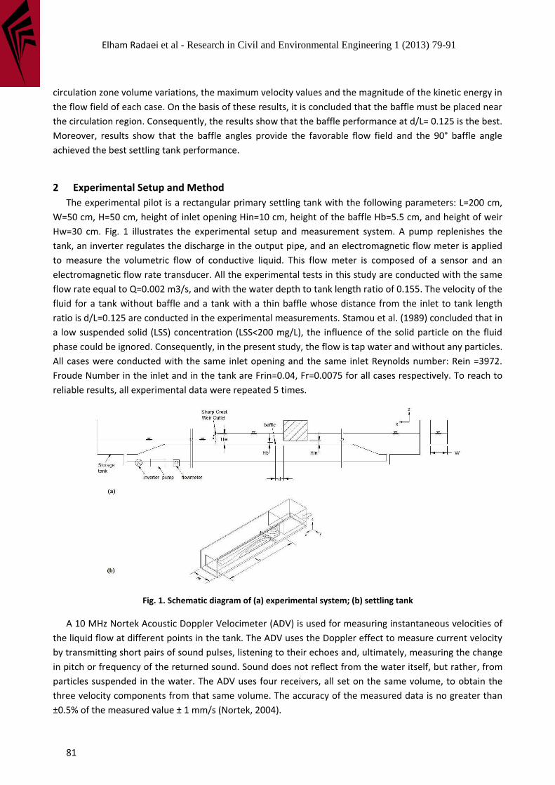
The experimental pilot is a rectangular primary settling tank with the following parameters: L=200 cm,
W=50 cm, H=50 cm, height of inlet opening Hin=10 cm, height of the baffle Hb=5.5 cm, and height of weir
Hw=30 cm. Fig. 1 illustrates the experimental setup and measurement system. A pump replenishes the
tank, an inverter regulates the discharge in the output pipe, and an electromagnetic flow meter is applied
to measure the volumetric flow of conductive liquid. This flow meter is composed of a sensor and an
electromagnetic flow rate transducer. All the experimental tests in this study are conducted with the same
flow rate equal to Q=0.002 m3/s, and with the water depth to tank length ratio of 0.155. The velocity of the
fluid for a tank without baffle and a tank with a thin baffle whose distance from the inlet to tank length
ratio is d/L=0.125 are conducted in the experimental measurements. Stamou et al. (1989) concluded that in
a low suspended solid (LSS) concentration (LSS<200 mg/L), the influence of the solid particle on the fluid
phase could be ignored. Consequently, in the present study, the flow is tap water and without any particles.
All cases were conducted with the same inlet opening and the same inlet Reynolds number: Rein =3972.
Froude Number in the inlet and in the tank are Frin=0.04, Fr=0.0075 for all cases respectively. To reach to
reliable results, all experimental data were repeated 5 times.
Fig. 1. Schematic diagram of (a) experimental system; (b) settling tank
A 10 MHz Nortek Acoustic Doppler Velocimeter (ADV) is used for measuring instantaneous velocities of
the liquid flow at different points in the tank. The ADV uses the Doppler effect to measure current velocity
by transmitting short pairs of sound pulses, listening to their echoes and, ultimately, measuring the change
in pitch or frequency of the returned sound. Sound does not reflect from the water itself, but rather, from
particles suspended in the water. The ADV uses four receivers, all set on the same volume, to obtain the
three velocity components from that same volume. The accuracy of the measured data is no greater than
±0.5% of the measured value ± 1 mm/s (Nortek, 2004).
Elham Radaei et al - Research in Civil and Environmental Engineering 1 (2013) 79-91
82
There are some assumptions when applying ADV in a turbidity flow. Firstly, the measured velocity by
ADV is related to the velocity of fine particles which are suspended in the fluid. In the other words ADV
measuring the change in frequency of the returned sound from fine particles suspended in the water. So it
is assumed that these fine particles move at the same velocity of the fluid. As mentioned before in this
research the tap water is used as a fluid, so for using ADV, very fine particles of kaolin with low
concentration were added as a seeding material to the water. The second one is the changes in density or
density layer of the fluid which cause changes in the acoustic velocity. Whereas the sediment concentration
in the dense fluid has an amount up to 15 g/l, the value of the sediment concentration is more lower than
this amount during the experiments, so there is not any significant changes in the acoustic velocity
(Kawanisi and Yokosi, 1997).
3 Computational Model
3.1 Time Average Flow Equation
Steady state incompressible flow conditions with viscosity and inertia effects are generally considered in
hydraulic numerical modeling. The Navier-Stokes equations have been well adapted to solve the governing
equations. These equations comprise an incompressible form of the conservation of mass and momentum
equations, as well as nonlinear advection, rate of change, diffusion, and source term in the partial
differential equation. Mass and momentum equations coupled via velocity can be used to derive an
equation for the pressure term. In a turbulent flow, the computations become more complex in the Navier-
Stokes equations. The modified form of the Navier-Stokes equations, including the Reynolds stress term,
which approximates the random turbulent fluctuations by statistics, is represented by the Reynolds-
Averaged Navier-Stokes (RANS) equations. Hence, the continuity and momentum equations are solved for
the steady, incompressible, turbulent, and isothermal flow. As the flow pattern is assumed to be two-
dimensional, two momentum equations in the x and z directions corresponding to the length and height of
the tank, respectively, were solved. The general mass continuity equation is expressed as (Hirt and Nichols,
1981; Hirt and Sicilian, 1985):
0f x z
V uA wA
t x z
(1)
where fV
is the fractional volume of flow in the calculation cell; is the fluid density; and u and v are
the velocity components in the length and height (x,z) directions, respectively. The momentum equation for
the fluid velocity components in the two directions are the Navier-Stokes equations, which is expressed as:
1 1
x z x x
f
u u u PuA wA G f
t V x z x
(2)
1 1
x z z z
f
w w w PuA wA G f
t V x z z
(3)
Where, ,
x zG G
are body accelerations, and ,
x zf f
are viscous accelerations that form a variable dynamic
viscosity µ given by:
Elham Radaei et al - Research in Civil and Environmental Engineering 1 (2013) 79-91
83
f x x xx z xzV f wsx A A
x z
(4)
f z x xz z zzV f wsz A A
x z
(5)
where:
2 , 2 ,xzx zx z
u w u w
x z z x
(6)
The terms wsx and wsz refer to wall shear stresses. If these terms are omitted, there would be no wall
shear stress because the remaining terms contain the fractional flow areas (Ax, Az) that vanish at walls. The
wall stresses are modelled by assuming a zero tangential velocity on the portion of any area close to the
flow. However, mesh boundaries are an exception because they can be assigned non-zero tangential
velocities. For turbulent flows, a law-of-the-wall velocity profile is assumed near the wall, which modifies
the wall shear stress magnitude (FlowScience, 2009).
The volume-of-fluid (VOF) method (Hirt and Nichols, 1981) is used to define the appropriate boundary
conditions on a free surface. The VOF method works by defining the volume of fluid within each discretized
cell. If a cell is empty, the value of F becomes equal to zero. However, if a cell is full, it receives a value of
F=1. If a cell contains the free surface, it receives a value between 0<F<1, which is correlated to the ratio of
fluid volume to cell volume. The water surface angle in the cell is determined by the location of the fluid in
surrounding cells. In essence, the location of the water surface within a cell is defined as a first-order
approximation, a straight line in 2D space and a plane surface in 3D space. Therefore, as the flow field is
calculated at each time step, the location of the free surface is updated, allowing the free surface to move
temporally and spatially.
10
x z
F
FFA u FA w
t V x z
(7)
F in one phase problem depicts the volume fraction filled by the fluid. Voids are regions without fluid
mass that have a uniform pressure appointed to them. Physically, they represent regions filled with a vapor
or gas whose density is insignificant compared to the fluid density.
3.2 Turbulence Model
A slightly more sophisticated (and more widely used) model is made up of two transport equations for
turbulent kinetic energy k and its dissipation ε. This is known as k-ε model (Harlow and Nakayama, 1967).
The k-ε model provides reasonable approximations of many types of flows, although it sometimes requires
modification of its dimensionless parameters (or even functional changes to terms in the equations)
(Svendsen and Kirby, 2004). The turbulence kinetic energy, k, and its rate of dissipation, ε, are obtained
from the following transport equations:
Elham Radaei et al - Research in Civil and Environmental Engineering 1 (2013) 79-91
84
1
x z
F
k k kuA wA P G Diff
t V x z
(8)
2
1
3 2
.1. .
x z
F
CuA wA P C G DDif C
t V x z k k
(9)
Where P is the turbulent kinetic energy production; G is the buoyancy production; Diff and DDif
represent diffusion; and C1ε, C2ε, and C3ε are constants. In a standard k-ε model, C1ε=1.44, C2ε=1.92, and
C3ε=0.2.
3.3 Numerical Model
The basis of the Flow-3D® flow solver is a finite volume or finite difference formulation, in Eulerian
framework, of the equations describing the conservation of mass, momentum, and energy in a fluid. The
code can simulate incompressible and compressible flow, as well as laminar and turbulent flows.
Flow-3D® solves the fully three-dimensional transient Navier-Stokes equations using the Fractional
Area/Volume Obstacle Representation (FAVOR) and the VOF method. The solver uses finite difference or
finite volume approximation to discretize the computational domain. Flow-3D® uses a simple grid of
rectangular elements, and as such, it has the advantages of ease of generation and regularity for improved
numerical accuracy. Moreover, it requires minimal memory storage. Geometry is then defined within the
grid by computing the fractional face areas and fractional volumes of each element blocked by obstacles.
For each cell, the mean values of the flow parameters such as pressure and velocity are determined at
discrete times. The new velocity in each cell is calculated from the coupled momentum and continuity
equation using previous time step values in each center of the cell face. The pressure term is gained and
adjusted using the estimated velocity to satisfy the continuity equation. With the computed velocity and
pressure for a later time, the remaining variables are estimated involving turbulent transport, density
advection and diffusion, and wall function evaluation.
The boundary condition for the inflow (influent) is the constant velocity, whereas those selected for the
outlet (effluent) is the outflow condition. No slip conditions were applied at the rigid walls, and these were
treated as non-penetrative boundaries. A law-of-the-wall velocity profile was assumed near the wall, which
modifies the wall shear stress magnitude.
The flow in the sedimentation tanks is actually three-dimensional, especially in the inlet section of the
tank. This is related to the position of the inlet and outlet of tank, as well as their opening sizes. For
simplicity, the flow field can be represented as two-dimensional vertical plane models because in the
current study, the inlet and outlet spread out all over the width of the tank. Some numerical simulations
were thus conducted with various numbers of cells to find the grid-independent solution. Finally, a 69×288
grid with approximately 19872 cells was chosen for the computation modeling.
4 Verification Test
In order to verify the result of computational model of the sedimentation tank, the experimental
measurements for two cases of sedimentation tank was considered: a settling tank without baffle and a
Elham Radaei et al - Research in Civil and Environmental Engineering 1 (2013) 79-91
85
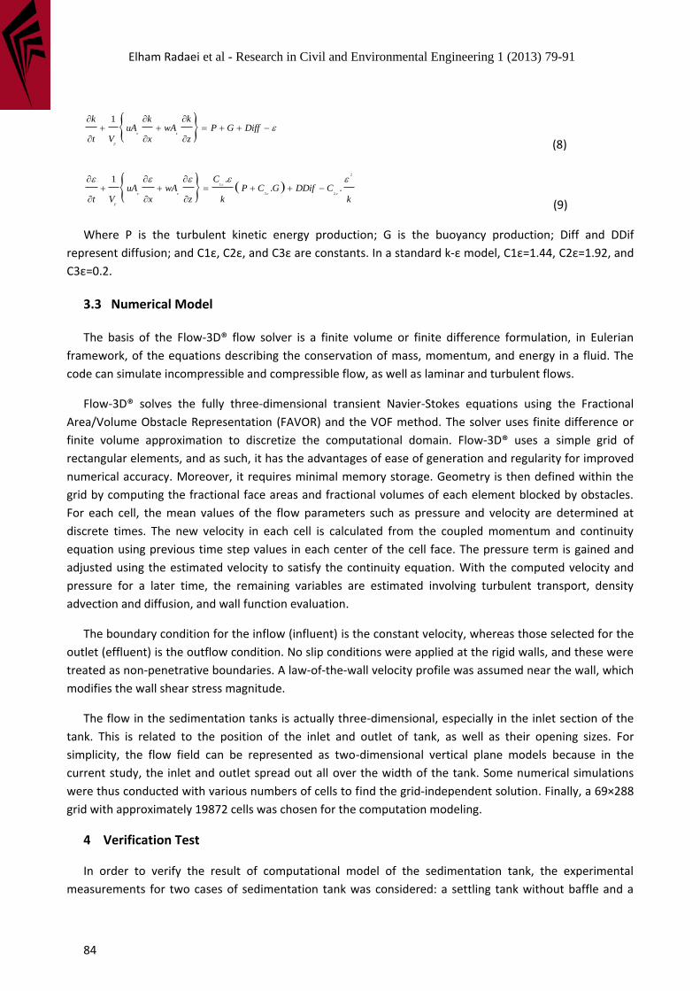
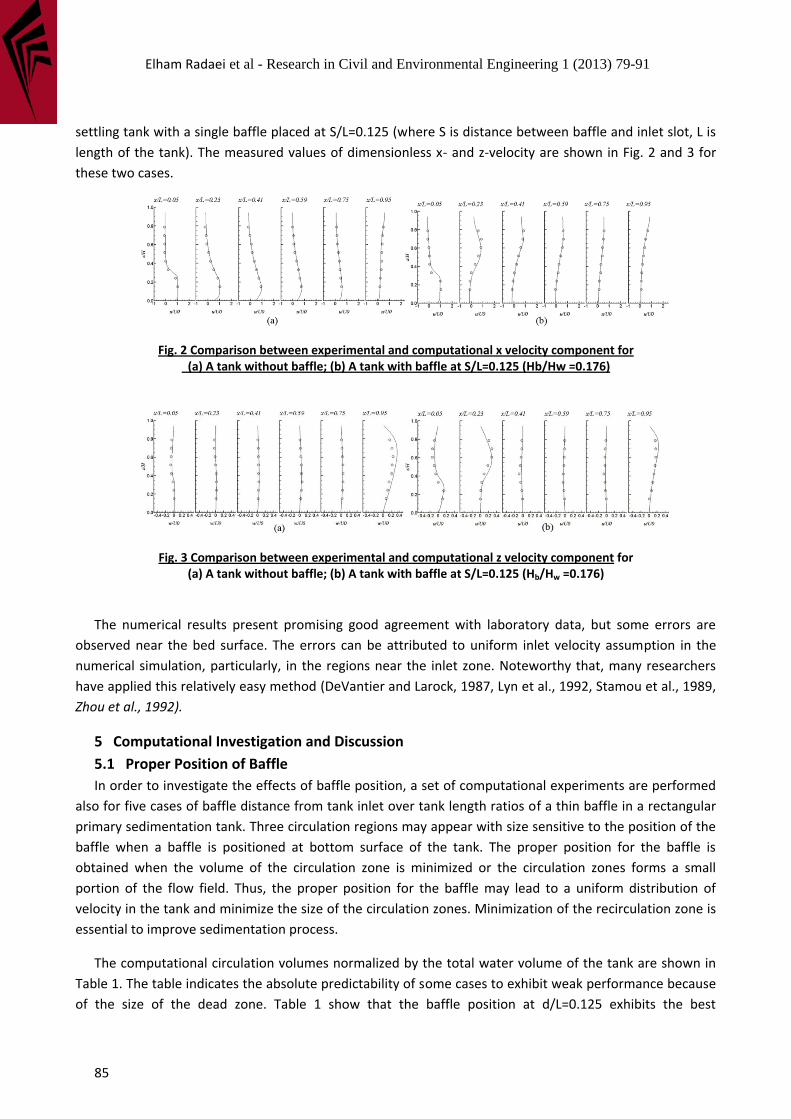
settling tank with a single baffle placed at S/L=0.125 (where S is distance between baffle and inlet slot, L is
length of the tank). The measured values of dimensionless x- and z-velocity are shown in Fig. 2 and 3 for
these two cases.
Fig. 2 Comparison between experimental and computational x velocity component for (a) A tank without baffle; (b) A tank with baffle at S/L=0.125 (Hb/Hw =0.176)
Fig. 3 Comparison between experimental and computational z velocity component for (a) A tank without baffle; (b) A tank with baffle at S/L=0.125 (Hb/Hw =0.176)
The numerical results present promising good agreement with laboratory data, but some errors are
observed near the bed surface. The errors can be attributed to uniform inlet velocity assumption in the
numerical simulation, particularly, in the regions near the inlet zone. Noteworthy that, many researchers
have applied this relatively easy method (DeVantier and Larock, 1987, Lyn et al., 1992, Stamou et al., 1989,
Zhou et al., 1992).
5 Computational Investigation and Discussion
5.1 Proper Position of Baffle
In order to investigate the effects of baffle position, a set of computational experiments are performed
also for five cases of baffle distance from tank inlet over tank length ratios of a thin baffle in a rectangular
primary sedimentation tank. Three circulation regions may appear with size sensitive to the position of the
baffle when a baffle is positioned at bottom surface of the tank. The proper position for the baffle is
obtained when the volume of the circulation zone is minimized or the circulation zones forms a small
portion of the flow field. Thus, the proper position for the baffle may lead to a uniform distribution of
velocity in the tank and minimize the size of the circulation zones. Minimization of the recirculation zone is
essential to improve sedimentation process.
The computational circulation volumes normalized by the total water volume of the tank are shown in
Table 1. The table indicates the absolute predictability of some cases to exhibit weak performance because
of the size of the dead zone. Table 1 show that the baffle position at d/L=0.125 exhibits the best
Elham Radaei et al - Research in Civil and Environmental Engineering 1 (2013) 79-91
86
performance. In addition, it is note that if baffle is located in worse position, the efficiency of this tank
maybe less than a tank without any baffle. Consequently, it is necessary to investigate about the best
position and configuration of the baffle in settling tank.
Table. 1 Computed normalized circulating volume for various position of the baffle (only for a baffle height, Hb/H=0.18)
d / L 0.10 0.125 0.150 0.20 0.25 W.B.
C.V. (%) 33.90 32.28 34.40 34.43 35.08 37.05
d : The baffle distance from the inlet of the tank L : The length of the tank W.B. : Without Baffle C.V. : Normalized Circulation Volume
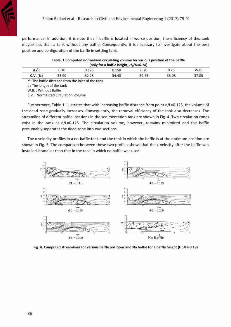
Furthermore, Table 1 illustrates that with increasing baffle distance from point d/L=0.125, the volume of
the dead zone gradually increases. Consequently, the removal efficiency of the tank also decreases. The
streamline of different baffle locations in the sedimentation tank are shown in Fig. 4. Two circulation zones
exist in the tank at d/L=0.125. The circulation volume, however, remains minimized and the baffle
presumably separates the dead zone into two sections.
The x-velocity profiles in a no-baffle tank and the tank in which the baffle is at the optimum position are
shown in Fig. 5. The comparison between these two profiles shows that the x-velocity after the baffle was
installed is smaller than that in the tank in which no baffle was used.
Fig. 4. Computed streamlines for various baffle positions and No baffle for a baffle height (Hb/H=0.18)
d/L=0.10
d/L = 0.120 d/L = 0.125
d/L = 0.135 d/L = 0.150
d/L = 0.200 d/L = 0.250
d/L = 0.300 d/L = 0.400
d/L = 0.120 d/L = 0.125
d/L = 0.135 d/L = 0.150
d/L = 0.200 d/L = 0.250
d/L = 0.300 d/L = 0.400
d/L = 0.120 d/L = 0.125
d/L = 0.135 d/L = 0.150
d/L = 0.200 d/L = 0.250
d/L = 0.300 d/L = 0.400
d/L = 0.120 d/L = 0.125
d/L = 0.135 d/L = 0.150
d/L = 0.200 d/L = 0.250
d/L = 0.300 d/L = 0.400
No Baffle
Elham Radaei et al - Research in Civil and Environmental Engineering 1 (2013) 79-91
87
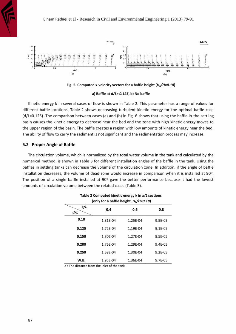
Fig. 5. Computed x-velocity vectors for a baffle height (Hb/H=0.18)
a) Baffle at d/L= 0.125, b) No baffle
Kinetic energy k in several cases of flow is shown in Table 2. This parameter has a range of values for
different baffle locations. Table 2 shows decreasing turbulent kinetic energy for the optimal baffle case
(d/L=0.125). The comparison between cases (a) and (b) in Fig. 6 shows that using the baffle in the settling
basin causes the kinetic energy to decrease near the bed and the zone with high kinetic energy moves to
the upper region of the basin. The baffle creates a region with low amounts of kinetic energy near the bed.
The ability of flow to carry the sediment is not significant and the sedimentation process may increase.
5.2 Proper Angle of Baffle
The circulation volume, which is normalized by the total water volume in the tank and calculated by the
numerical method, is shown in Table 3 for different installation angles of the baffle in the tank. Using the
baffles in settling tanks can decrease the volume of the circulation zone. In addition, if the angle of baffle
installation decreases, the volume of dead zone would increase in comparison when it is installed at 90º.
The position of a single baffle installed at 90º gave the better performance because it had the lowest
amounts of circulation volume between the related cases (Table 3).
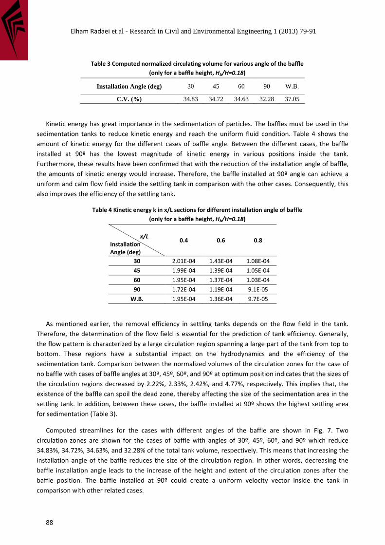
Table 2 Computed kinetic energy k in x/L sections
(only for a baffle height, Hb/H=0.18)
x/L
d/L 0.4 0.6 0.8
0.10 1.81E-04 1.25E-04 9.5E-05
0.125 1.72E-04 1.19E-04 9.1E-05
0.150 1.80E-04 1.27E-04 9.5E-05
0.200 1.76E-04 1.29E-04 9.4E-05
0.250 1.68E-04 1.30E-04 9.2E-05
W.B. 1.95E-04 1.36E-04 9.7E-05
X : The distance from the inlet of the tank
(a)
(b)
(a)
(b)
Elham Radaei et al - Research in Civil and Environmental Engineering 1 (2013) 79-91
88
Table 3 Computed normalized circulating volume for various angle of the baffle
(only for a baffle height, Hb/H=0.18)
Installation Angle (deg) 30 45 60 90 W.B.
C.V. (%) 34.83 34.72 34.63 32.28 37.05
Kinetic energy has great importance in the sedimentation of particles. The baffles must be used in the
sedimentation tanks to reduce kinetic energy and reach the uniform fluid condition. Table 4 shows the
amount of kinetic energy for the different cases of baffle angle. Between the different cases, the baffle
installed at 90º has the lowest magnitude of kinetic energy in various positions inside the tank.
Furthermore, these results have been confirmed that with the reduction of the installation angle of baffle,
the amounts of kinetic energy would increase. Therefore, the baffle installed at 90º angle can achieve a
uniform and calm flow field inside the settling tank in comparison with the other cases. Consequently, this
also improves the efficiency of the settling tank.
Table 4 Kinetic energy k in x/L sections for different installation angle of baffle
(only for a baffle height, Hb/H=0.18)
x/L
Installation Angle (deg)
0.4 0.6 0.8
30 2.01E-04 1.43E-04 1.08E-04
45 1.99E-04 1.39E-04 1.05E-04
60 1.95E-04 1.37E-04 1.03E-04
90 1.72E-04 1.19E-04 9.1E-05
W.B. 1.95E-04 1.36E-04 9.7E-05
As mentioned earlier, the removal efficiency in settling tanks depends on the flow field in the tank.
Therefore, the determination of the flow field is essential for the prediction of tank efficiency. Generally,
the flow pattern is characterized by a large circulation region spanning a large part of the tank from top to
bottom. These regions have a substantial impact on the hydrodynamics and the efficiency of the
sedimentation tank. Comparison between the normalized volumes of the circulation zones for the case of
no baffle with cases of baffle angles at 30º, 45º, 60º, and 90º at optimum position indicates that the sizes of
the circulation regions decreased by 2.22%, 2.33%, 2.42%, and 4.77%, respectively. This implies that, the
existence of the baffle can spoil the dead zone, thereby affecting the size of the sedimentation area in the
settling tank. In addition, between these cases, the baffle installed at 90º shows the highest settling area
for sedimentation (Table 3).
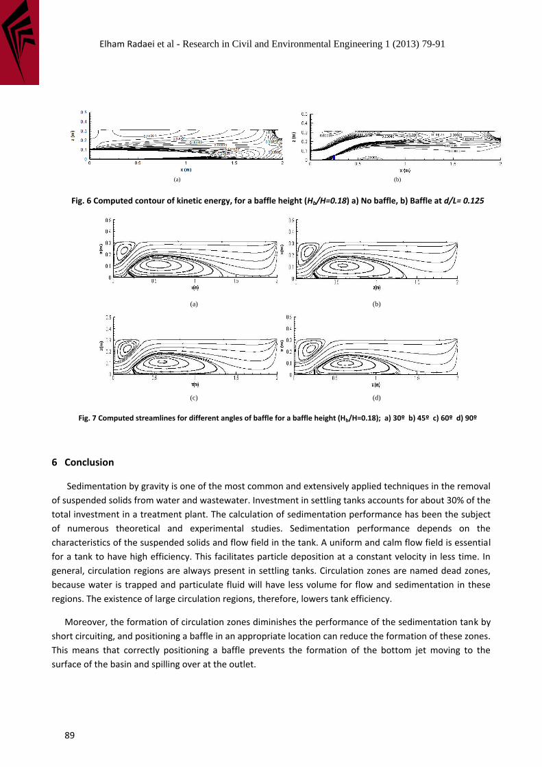
Computed streamlines for the cases with different angles of the baffle are shown in Fig. 7. Two
circulation zones are shown for the cases of baffle with angles of 30º, 45º, 60º, and 90º which reduce
34.83%, 34.72%, 34.63%, and 32.28% of the total tank volume, respectively. This means that increasing the
installation angle of the baffle reduces the size of the circulation region. In other words, decreasing the
baffle installation angle leads to the increase of the height and extent of the circulation zones after the
baffle position. The baffle installed at 90º could create a uniform velocity vector inside the tank in
comparison with other related cases.
Elham Radaei et al - Research in Civil and Environmental Engineering 1 (2013) 79-91
89
Fig. 6 Computed contour of kinetic energy, for a baffle height (Hb/H=0.18) a) No baffle, b) Baffle at d/L= 0.125
Fig. 7 Computed streamlines for different angles of baffle for a baffle height (Hb/H=0.18); a) 30º b) 45º c) 60º d) 90º
6 Conclusion
Sedimentation by gravity is one of the most common and extensively applied techniques in the removal
of suspended solids from water and wastewater. Investment in settling tanks accounts for about 30% of the
total investment in a treatment plant. The calculation of sedimentation performance has been the subject
of numerous theoretical and experimental studies. Sedimentation performance depends on the
characteristics of the suspended solids and flow field in the tank. A uniform and calm flow field is essential
for a tank to have high efficiency. This facilitates particle deposition at a constant velocity in less time. In
general, circulation regions are always present in settling tanks. Circulation zones are named dead zones,
because water is trapped and particulate fluid will have less volume for flow and sedimentation in these
regions. The existence of large circulation regions, therefore, lowers tank efficiency.
Moreover, the formation of circulation zones diminishes the performance of the sedimentation tank by
short circuiting, and positioning a baffle in an appropriate location can reduce the formation of these zones.
This means that correctly positioning a baffle prevents the formation of the bottom jet moving to the
surface of the basin and spilling over at the outlet.
(a)
(a)
(b)
(b)
(a)
(a)
(b)
(b)
(a) (b)
(c) (d)
Elham Radaei et al - Research in Civil and Environmental Engineering 1 (2013) 79-91
90
Numerical approaches were carried out to investigate the effects of baffle location and baffle height on
the flow field. With CFD and VOF methods, a numerical simulation was developed for the flow in the tank
through the FLOW-3D® software. Results show that the installation of a baffle improves tank efficiency in
terms of sedimentation. A baffle also reduces kinetic energy and induces a decrease in maximum
magnitude of the stream-wise velocity and upward inclination of the velocity field compared with the no-
baffle tank. On the basis of these results, it is concluded that the baffle must be placed near the circulation
region. Results also show that installing a baffle at an angel of 90° led to a reduction in the size of the
circulation zone, kinetic energy, and maximum velocity magnitude, and created a uniform velocity vector
inside the settling zone compared with other baffle angles. Consequently, the 90° baffle angle achieved the
best tank performance.
References
Abdel-Gawad, S.M.&McCorquodale, J.A. (1984). Strip integral method applied to settling tanks. Journal of hydraulic engineering, 110(1), 1-17.
Al-Sammarraee, M., Chan, A., Salim, S.&Mahabaleswar, U. (2009). Large-eddy simulations of particle sedimentation in a longitudinal sedimentation basin of a water treatment plant. Part i: Particle settling performance. Chemical Engineering Journal, 152(2), 307-314.
Bretscher, U., Krebs, P.&Hager, W.H. (1992). Improvement of flow in final settling tanks. Journal of Environmental Engineering, 118(3), 307-321.
Celik, I., Rodi, W.&Stamou, A. (1985). Prediction of hydrodynamic characteristics of rectangular settling tanks, In Proceeding international Symposium of Refined Flow Modeling and Turbulent Measurements, Iowa City, IA, USA, pp. 641-651.
FlowScience (2009). Flow-3d user manual, Ver. 9.4.1 ed, Santa Fe, NM, USA.
Goula, A.M., Kostoglou, M., Karapantsios, T.D.&Zouboulis, A.I. (2008). A cfd methodology for the design of sedimentation tanks in potable water treatment: Case study: The influence of a feed flow control baffle. Chemical Engineering Journal, 140(1), 110-121.
Harlow, F.H.&Nakayama, P.I. (1967). Turbulence transport equations. Phys. of Fluids, 10(11), 2323-2333.
Hirt, C.W.&Nichols, B.D. (1981). Volume of fluid (vof) method for the dynamics of free boundaries. J. Comp. Phys., 39, 201-225.
Hirt, C.W.&Sicilian, J.M. (1985). A porosity technique for the definition of obstacles in rectangular cell meshes, In Fourth International Conf. Ship Hydro. National Academy of Science, Washington, DC, pp. 1-19.
Imam, E., McCorquodale, J.A.&Bewtra, J.K. (1983). Numerical modeling of sedimentation tanks. Journal of hydraulic engineering, 109(12), 1740-1754.
Kawanisi, K.&Yokosi, S. (1997). Measurements of suspended sediment and turbulence in tidal boundary layer. Continental Shelf Research, 17, 859-875.
Larsen, P. (1977). Gotthardson, s.,om sedimenteringsgassangers hydraulic. Bulletin erie A. Nr. Inst. For Tekniks Vattenresurslare, Lund, Sweden (in Swedish).
Metcalf, I. (2003). Wastewater engineering; treatment and reuse. McGraw-Hill.
Nortek (2004). Nortek vectorino velocimeter-user guide,.
Elham Radaei et al - Research in Civil and Environmental Engineering 1 (2013) 79-91
91
Razmi, A., Firoozabadi, B.&Ahmadi, G. (2009). Experimental and numerical approach to enlargement of performance of primary settling tanks. Journal of Applied Fluid Mechanics, 2(1), 1-12.
Schamber, D.R.&Larock, B.E. (1981). Numerical analysis of flow in sedimentation basins. Journal of the Hydraulics Division, 107(5), 575-591.
Stamou, A., Adams, E.&Rodi, W. (1989). Numerical modeling of flow and settling in primary rectangular clarifiers. Journal of hydraulic research, 27(5), 665-682.
Svendsen, I.&Kirby, J. (2004). Numerical study of a turbulent hydraulic jump, In 17th ASCE Engineering Mechanics Conference, University of Delaware, Newmark, DE.