real-time feature extraction of the voice for musical … · real-time feature extraction of the...
TRANSCRIPT
REAL-TIME FEATURE EXTRACTION OF THE VOICE
FOR MUSICAL CONTROL
by
Adam Kestian
M.M., New York University, 2008
B.F.A, University of Michigan, 2006
a Thesis submitted in partial fulfillment
of the requirements for the degree of
Master of Science
in the School
of
Computing Science
c� Adam Kestian 2010
SIMON FRASER UNIVERSITY
Fall 2010
All rights reserved. This work may not bereproduced in whole or in part, by photocopy
or other means, without the permission of the author.

Last revision: Spring 09
Declaration of Partial Copyright Licence The author, whose copyright is declared on the title page of this work, has granted to Simon Fraser University the right to lend this thesis, project or extended essay to users of the Simon Fraser University Library, and to make partial or single copies only for such users or in response to a request from the library of any other university, or other educational institution, on its own behalf or for one of its users.
The author has further granted permission to Simon Fraser University to keep or make a digital copy for use in its circulating collection (currently available to the public at the “Institutional Repository” link of the SFU Library website <www.lib.sfu.ca> at: <http://ir.lib.sfu.ca/handle/1892/112>) and, without changing the content, to translate the thesis/project or extended essays, if technically possible, to any medium or format for the purpose of preservation of the digital work.
The author has further agreed that permission for multiple copying of this work for scholarly purposes may be granted by either the author or the Dean of Graduate Studies.
It is understood that copying or publication of this work for financial gain shall not be allowed without the author’s written permission.
Permission for public performance, or limited permission for private scholarly use, of any multimedia materials forming part of this work, may have been granted by the author. This information may be found on the separately catalogued multimedia material and in the signed Partial Copyright Licence.
While licensing SFU to permit the above uses, the author retains copyright in the thesis, project or extended essays, including the right to change the work for subsequent purposes, including editing and publishing the work in whole or in part, and licensing other parties, as the author may desire.
The original Partial Copyright Licence attesting to these terms, and signed by this author, may be found in the original bound copy of this work, retained in the Simon Fraser University Archive.
Simon Fraser University Library Burnaby, BC, Canada
Abstract
Voiced vowel production in human speech depends both on the oscillation of vocal
folds and the vocal tract shape, the latter contributing to the appearance of formants
in the spectrum of the speech signal. Many speech synthesis models use feed-forward
source-filter models, where the magnitude frequency response of the vocal tract is
approximated by the spectral envelope of the speech signal.
This thesis introduces a new model analysis method to identify the vocal tract
area function where the users formants are extracted and then matched to a piecewise
cylindrical waveguide model shape that produces similar spectra. When a match is
found, the corresponding model shape is provided to the user. Considerations are
made to improve feedback by tracking formant movement over time to account for
unintended action such as dropped formants or the wavering of an untrained voice.
iii
Contents
Approval ii
Abstract iii
Contents iv
List of Figures vi
1 Introduction 1
1.1 Thesis structure . . . . . . . . . . . . . . . . . . . . . . . . . . . . . . 3
2 Speech Production / Synthesis 4
2.1 Speech Production Process . . . . . . . . . . . . . . . . . . . . . . . . 4
2.2 Synthesis History . . . . . . . . . . . . . . . . . . . . . . . . . . . . . 5
2.2.1 Source-filter model of speech . . . . . . . . . . . . . . . . . . . 8
2.2.2 Digital Waveguide Model . . . . . . . . . . . . . . . . . . . . . 10
3 Feature Extraction 13
3.1 General Features/Background . . . . . . . . . . . . . . . . . . . . . . 13
3.1.1 Spectrum-based Low-level Features . . . . . . . . . . . . . . . 14
3.1.2 Time domain low-level features . . . . . . . . . . . . . . . . . 17
3.1.3 Spectral Envelope . . . . . . . . . . . . . . . . . . . . . . . . . 20
3.2 Vocal Tract Extraction/History . . . . . . . . . . . . . . . . . . . . . 24
3.2.1 Spectrum Relationship to Model . . . . . . . . . . . . . . . . . 24
3.2.2 Previous Vocal Tract Shape Estimation Methods . . . . . . . 27
iv
3.2.3 Motivation for New Approach . . . . . . . . . . . . . . . . . . 29
4 Estimation of Vocal Tract Shape 32
4.1 Formant Tracking . . . . . . . . . . . . . . . . . . . . . . . . . . . . . 34
4.1.1 Real-Time Considerations . . . . . . . . . . . . . . . . . . . . 35
4.2 Minimum Action for Improved Usability . . . . . . . . . . . . . . . . 37
4.3 Vocal Tract Estimation . . . . . . . . . . . . . . . . . . . . . . . . . . 41
4.4 Observations . . . . . . . . . . . . . . . . . . . . . . . . . . . . . . . . 43
5 Conclusions and Future Work 45
5.1 Future Work . . . . . . . . . . . . . . . . . . . . . . . . . . . . . . . . 47
Bibliography 49
v
List of Figures
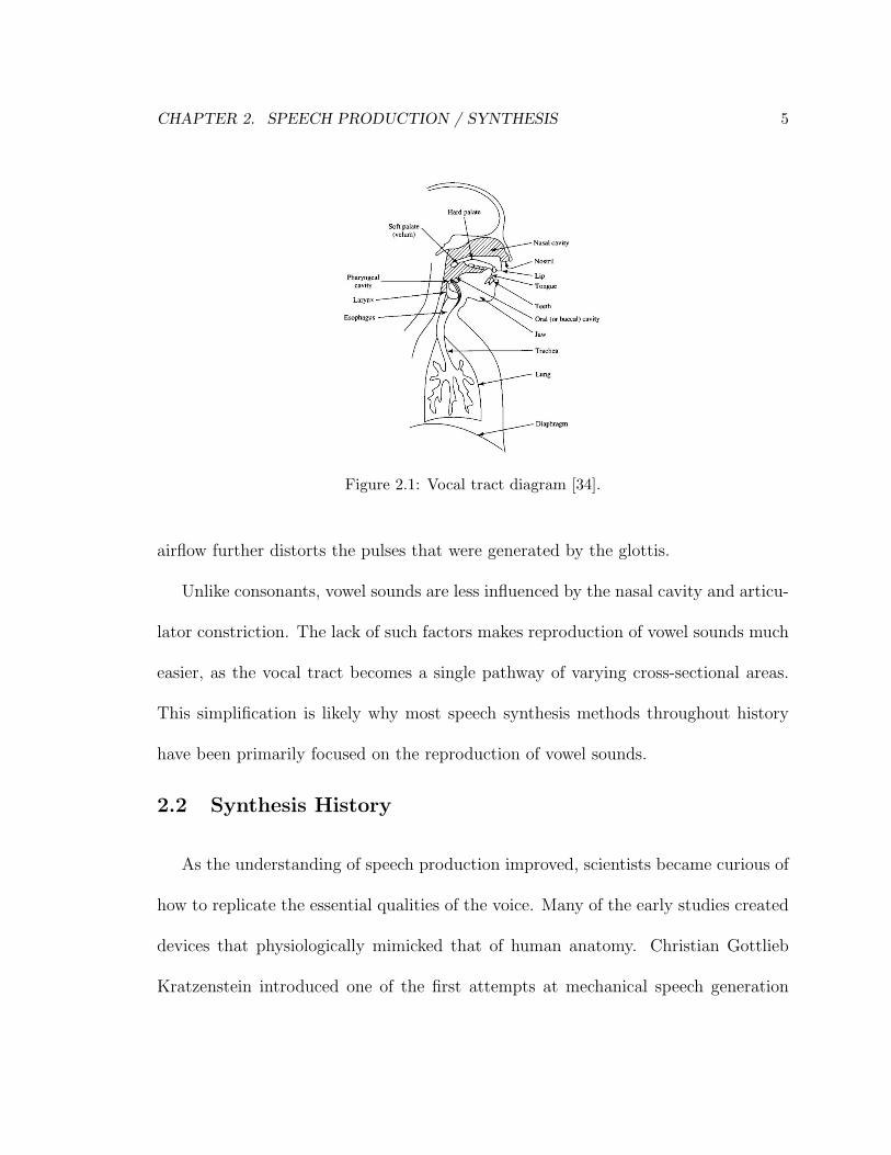
2.1 Vocal tract diagram [34]. . . . . . . . . . . . . . . . . . . . . . . . . . 5
2.2 General Vocoder block diagram . . . . . . . . . . . . . . . . . . . . . 8
2.3 Generalized source-filter model diagram . . . . . . . . . . . . . . . . . 9
2.4 Input pressure X(z) is fed to a vocal tract model of a M -segment,
one-dimensional digital waveguide. At changes in cross-sectional area,
the incoming pressure p is reflected and transmitted as a function of
the reflection coefficient k. The reflection functions R0(ω) and RL(ω)
determine how pressure is reflected and transmitted at the glottis and
lips, respectively. . . . . . . . . . . . . . . . . . . . . . . . . . . . . . 10
3.1 Spectrum-based features of voiced speech. Calm voiced speech pro-
duces relatively low spectral centroid, spread, and flatness measures. . 14
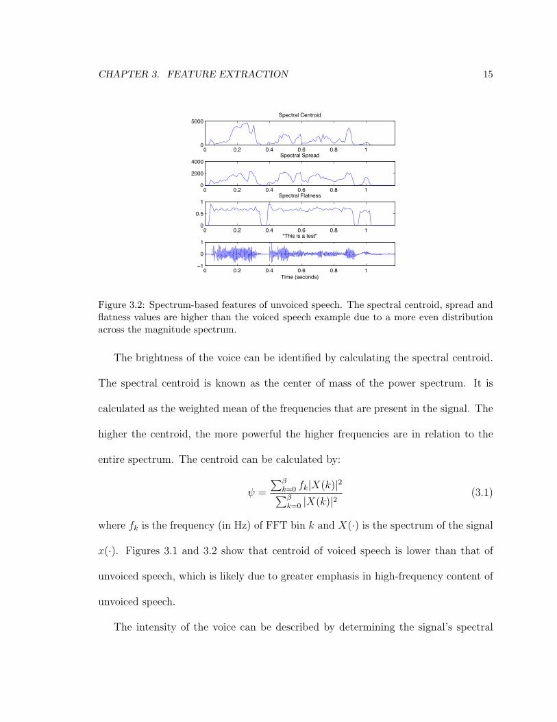
3.2 Spectrum-based features of unvoiced speech. The spectral centroid,
spread and flatness values are higher than the voiced speech example
due to a more even distribution across the magnitude spectrum. . . . 15
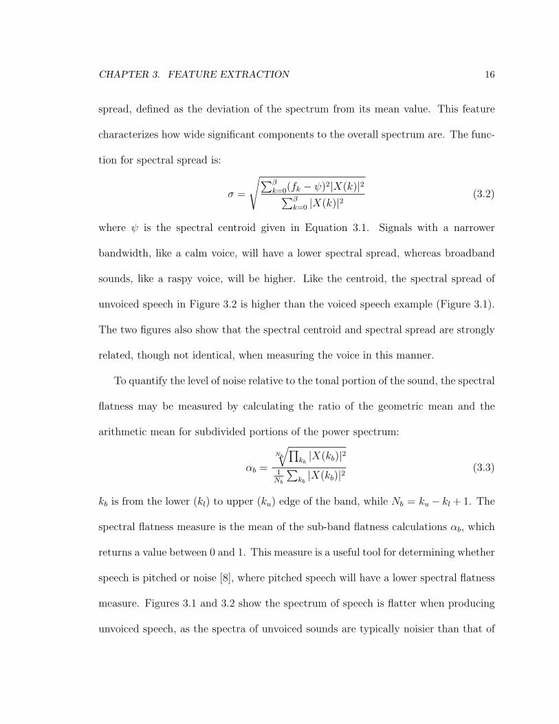
3.3 Time domain features of voiced speech. The local energy provides
a smoothed representation of the amplitude envelope, while a high
temporal centroid value corresponds to a sustained tone. . . . . . . . 18
3.4 Spectral envelopes obtained via LPC with varying orders . . . . . . . 20
3.5 Two segment piecewise cylindrical waveguide model . . . . . . . . . . 24
3.6 Pole location relative to reflection coefficient . . . . . . . . . . . . . . 25
3.7 Vocal tract shape estimation of synthesized examples . . . . . . . . . 28
3.8 Average reconstruction example . . . . . . . . . . . . . . . . . . . . . 31
4.1 Peak-picking example . . . . . . . . . . . . . . . . . . . . . . . . . . . 34
vi
4.2 Stream selection example . . . . . . . . . . . . . . . . . . . . . . . . . 36
4.3 Formant drop replacement then stream smoothing . . . . . . . . . . . 38
4.4 Singing example /ee/ - /oo/ - /ee/ . . . . . . . . . . . . . . . . . . . 40
4.5 Average result of the proposed algorithm . . . . . . . . . . . . . . . . 41
4.6 Estimation of vocal tract shape for vowel sound /au/ . . . . . . . . . 43
4.7 Estimation of vocal tract shape for vowel sound /ee/ . . . . . . . . . 44
5.1 Pure Data object displaying /au/ example . . . . . . . . . . . . . . . 47
vii
Chapter 1
Introduction
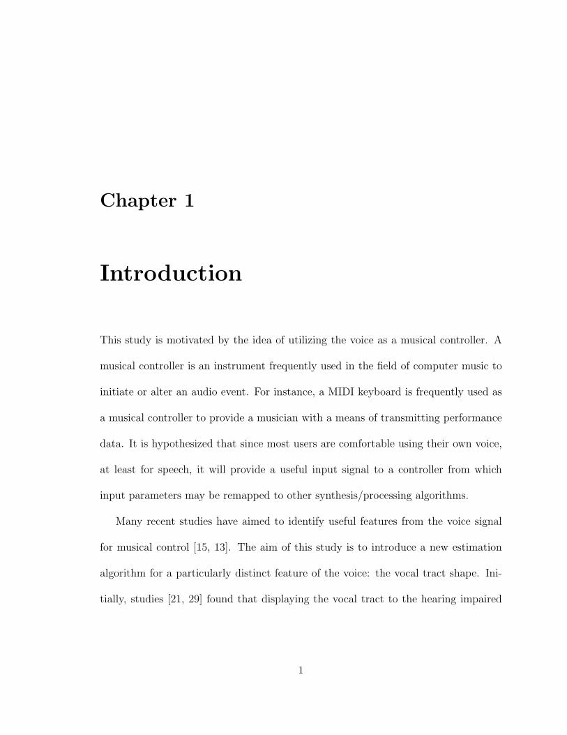
This study is motivated by the idea of utilizing the voice as a musical controller. A
musical controller is an instrument frequently used in the field of computer music to
initiate or alter an audio event. For instance, a MIDI keyboard is frequently used as
a musical controller to provide a musician with a means of transmitting performance
data. It is hypothesized that since most users are comfortable using their own voice,
at least for speech, it will provide a useful input signal to a controller from which
input parameters may be remapped to other synthesis/processing algorithms.
Many recent studies have aimed to identify useful features from the voice signal
for musical control [15, 13]. The aim of this study is to introduce a new estimation
algorithm for a particularly distinct feature of the voice: the vocal tract shape. Ini-
tially, studies [21, 29] found that displaying the vocal tract to the hearing impaired
1
CHAPTER 1. INTRODUCTION 2
can improve their overall speech performance, as well as being an effective instruc-
tional tool for singers [26]. More recently, some have identified the vocal tract shape
as a potential feature for musical control and have used vision-based methods for its
estimation [10, 20].
There are numerous proposed vocal tract estimation methods [29, 36, 19]. Most
of these algorithms base their findings by considering the voice a source-filter model,
where the vocal tract is a linear time-invariant filter that influences the spectral con-
tent of the voice. By changing the shape of the vocal tract, unique spectra is produced,
thereby generating a distinct sound (phoneme). One spectral characteristic that is
strongly correlated to shape are formants, spectral peaks of the sound spectrum caused
by resonances of the vocal tract.
Previous vocal tract estimation algorithms either produce inconsistent results or
are too computationally expensive for real-time applications. This study introduces
an efficient and accurate vocal tract estimation algorithm that identifies the area
function by comparing the user’s formants to those generated by a vocal tract model.
Here, the formants generated by each shape of the vocal tract model are stored in
a database offline to reduce the number of real-time calculations. The best formant
match between the user and collection of model shapes is identified as the correspond-
ing area function. A parameter is made available to adjust the algorithm’s sensitivity
to change in the produced sound; sensitivity can be reduced for novice users and
later increased for the estimation of more subtle nuances. In doing so, the sensitivity
CHAPTER 1. INTRODUCTION 3
parameter offers a customizable level of depth, which the author believes will allow
the algorithm to provide useful feedback for users of varying abilities.
1.1 Thesis structure
The thesis begins by examining the principles of speech production and the analysis
features that have led to the development of current speech models. Chapter 3 pro-
vides a review of several feature extraction methods which have previously been used
to generate input/control parameters, as well as an examination of how particular
features relate to the piecewise cylindrical waveguide model of the voice. Chapter
4 describes a new vocal tract area function estimation algorithm that matches the
user’s formants to those generated by a particular cylindrical waveguide shape. This
chapter also details performance considerations regarding feedback for users of vary-
ing abilities. Chapter 5 provides an implementation of the algorithm in the real-time
graphical programming environment Pure Data (PD) [1], as well as potential avenues
for algorithm improvements.
Chapter 2
Speech Production / Synthesis
2.1 Speech Production Process
In general terms, speech is generated by the coupling of oscillating vocal folds to the
vocal tract, the shape of which may change during speech. The vocal tract consists
of the laryngeal cavity, the pharynx, the oral cavity, and the nasal cavity. Figure 2.1
identifies these principle components of the vocal tract that impact speech production.
Speech production begins when the lungs supply additional pressure to the vocal tract.
The glottal folds, within the laryngeal cavity at the base of the vocal tract, open and
close periodically, thereby modulating the airflow from the lungs. This airflow then
propagates throughout the vocal tract in a path that is dependent on what sound is
to be generated.
Typically, all chambers of the vocal tract are utilized when producing consonant
sounds. When producing fricative consonants, two articulators1 in the oral cavity are
placed closely together thereby forcing air through a narrow channel. This turbulent
1Articulators are points within the vocal tract where obstruction occurs. Generally, this obstruction is aresult of an active articulator, like the tongue, contact a passive articulator like the teeth.
4
CHAPTER 2. SPEECH PRODUCTION / SYNTHESIS 5
Figure 2.1: Vocal tract diagram [34].
airflow further distorts the pulses that were generated by the glottis.
Unlike consonants, vowel sounds are less influenced by the nasal cavity and articu-
lator constriction. The lack of such factors makes reproduction of vowel sounds much
easier, as the vocal tract becomes a single pathway of varying cross-sectional areas.
This simplification is likely why most speech synthesis methods throughout history
have been primarily focused on the reproduction of vowel sounds.
2.2 Synthesis History
As the understanding of speech production improved, scientists became curious of
how to replicate the essential qualities of the voice. Many of the early studies created
devices that physiologically mimicked that of human anatomy. Christian Gottlieb
Kratzenstein introduced one of the first attempts at mechanical speech generation

CHAPTER 2. SPEECH PRODUCTION / SYNTHESIS 6
[14] in 1779 at the Imperial Academy of St. Petersberg. Kratzenstein constructed
a series of resonators to emulate the vocal tract shapes for five vowels. The lungs
were simulated via an air passage that was connected to a glottis-like vibrating reed.
This reed produced periodic pulses that were influenced by the attached resonators
to produce the appropriate vowel sound.
Shortly thereafter, Wolfgang von Kempelen demonstrated a machine [9] in 1791
that was capable of concatenating a variety of utterances. The machine utilized
bellows which supplied air to a reed. This reed was attached to a flexible leather
resonator that could produce variable voiced sounds based on its shape, which could
be manipulated by the user’s hand. This device also had mechanisms in place to
simulate the nasal cavity, as well as fricative sounds produced by the teeth and lips.
In 1841, former astronomer Joseph Faber introduced “Euphonia”; a physiologically
accurate device that included a head to which the sounds were emitted from. A piano-
like device of fourteen keys were positioned next to the machine. These keys controlled
the position of the jaw, lips, and tongue. A bellows and an ivory reed were connected
to the head to simulate the lungs and larynx. The machine was capable of pronouncing
a wide variety of words in many European languages, though was hindered by poor
diction and its monotonous voice [12].
Throughout the 1800s, scientists were divided about the purpose of voice synthe-
sis. Was it an attempt to create representative sounds from physiologically accurate
models like Kratzenstein or to reproduce audibly equivalent sounds like Kempelen?
CHAPTER 2. SPEECH PRODUCTION / SYNTHESIS 7
For those that only sought after audible equivalency, voice “features” quickly became
the main elements of their synthesis techniques.
British engineers William H. Preece and August Stroh created vowel synthesis
devices in the 1870s based on the work of Hermann von Helmholtz; who prescribed
resonating frequencies to match particular vowel sounds [16]. The most famous of
these devices was the automatic phonograph, where the trajectories for resonant fre-
quencies of a given vowel sound were etched into brass discs and then reproduced via
a phonograph.
While scientists like John Q. Stewart were still developing analogs of the vocal
organs [33] in the early 1900s, the majority of synthesis techniques favored were
feature-based. Some elements of these methods are still prominently used today.
Electronic and acoustic engineer Homer W. Dudley introduced Bell Lab’s first voice
synthesizer known as the “Vocoder” [24], which reproduced an audio signal through
bandpass filtering the signal. The Vocoder was developed to compress speech that
was to be sent over communication lines during World War II. Instead of sending a
significant amount of speech data, the voice was simplified to features, which could
be efficiently sent and then reproduced at the receiver.
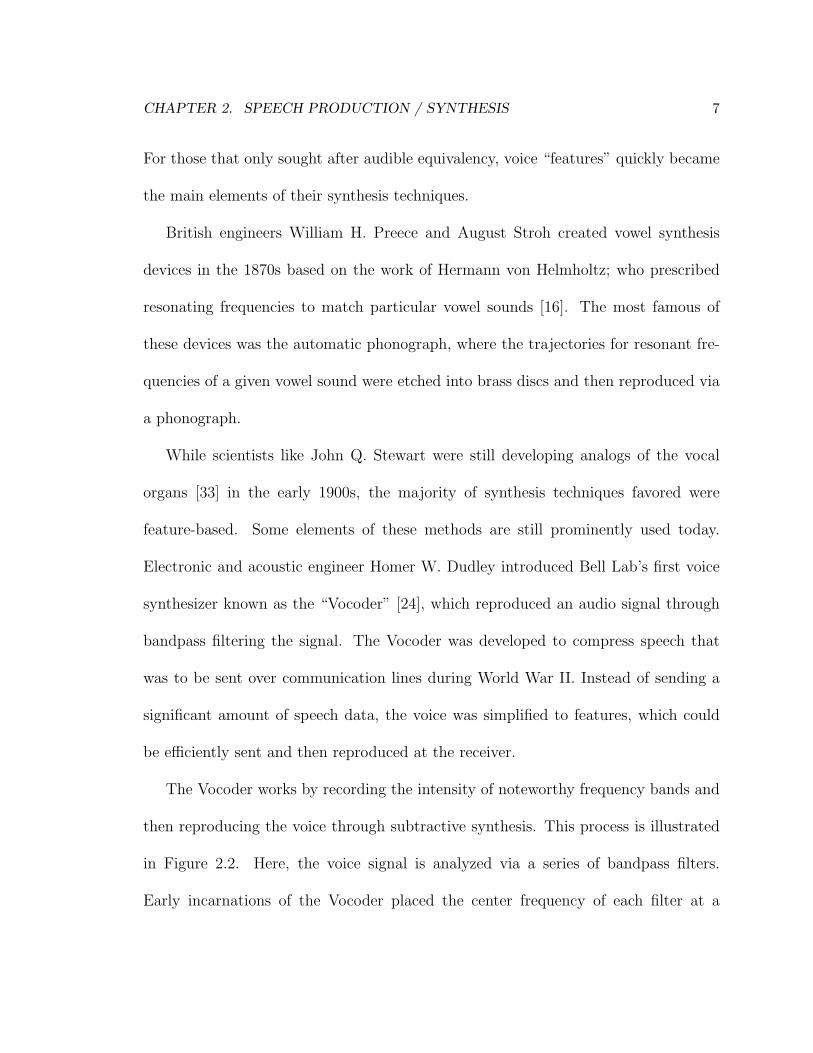
The Vocoder works by recording the intensity of noteworthy frequency bands and
then reproducing the voice through subtractive synthesis. This process is illustrated
in Figure 2.2. Here, the voice signal is analyzed via a series of bandpass filters.
Early incarnations of the Vocoder placed the center frequency of each filter at a
CHAPTER 2. SPEECH PRODUCTION / SYNTHESIS 8
Figure 2.2: General Vocoder block diagram
fixed location. The response of these filters recorded the amplitude envelope for
that particular spectral region. At the receiver’s end, a synthesized glottal source
(carrier) is then filtered based on the amplitude envelopes that were sent over the
communication line to resynthesize the voice signal. At the World’s Fair in 1939, an
operator controlled variation of the Vocoder known as the “Voder” was shown, where
the source, pitch, formant locations, and stop presets could all be altered to create
different voice sounds. Both the Vocoder and Voder were not only important in their
contributions to the field of voice resynthesis, but also the evolution of the source-filter
model.
2.2.1 Source-filter model of speech
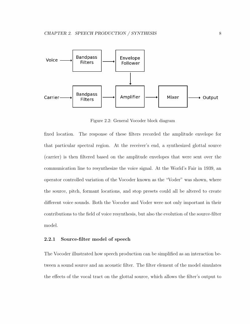
The Vocoder illustrated how speech production can be simplified as an interaction be-
tween a sound source and an acoustic filter. The filter element of the model simulates
the effects of the vocal tract on the glottal source, which allows the filter’s output to
CHAPTER 2. SPEECH PRODUCTION / SYNTHESIS 9
Figure 2.3: Generalized source-filter model diagram
represent the radiated acoustic pressure from the mouth. Figure 2.3 depicts a gener-
alized source-filter model, though its implementation varies based on certain model
assumptions. Each implementation of the model can make separate assumptions on
the linearity and time-invariance of the filter. It is assumed that the vocal tract is
a linear acoustic system which by definition means it adheres to both the scaling
property:
L{gx(·)} = gL{x(·)} (2.1)
and the superposition property.
L{x1(·) + x2(·)} = L{x1(·)} + L{x2(·)} (2.2)
where L denotes a linear system. Studies [27] have shown that the vocal tract is
essentially linear due to the negligible influence of the softer walls, such as the cheeks
or velum, on general approximations.
The source-filter model of the vocal tract is time invariant if its behavior is in-
dependent of time. That is, if the input signal x(n) produces an output y(n), then
CHAPTER 2. SPEECH PRODUCTION / SYNTHESIS 10
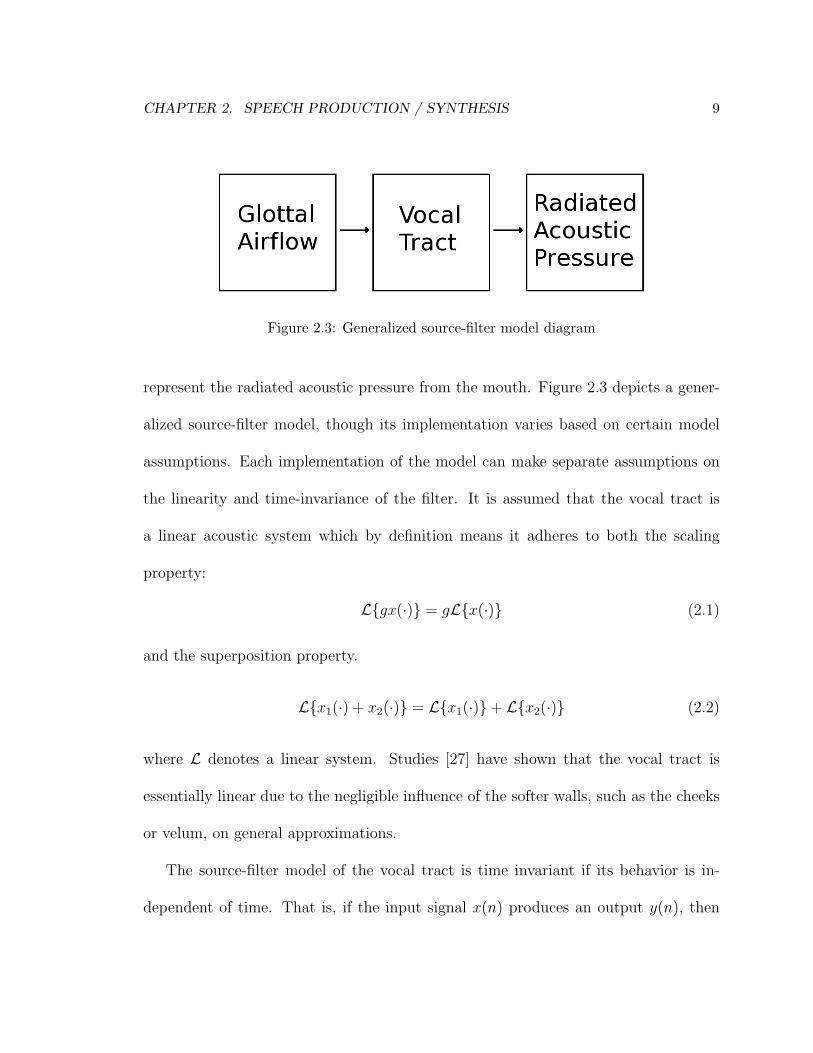
Figure 2.4: Input pressure X(z) is fed to a vocal tract model of a M -segment, one-dimensional digital waveguide. At changes in cross-sectional area, the incoming pressurep is reflected and transmitted as a function of the reflection coefficient k. The reflectionfunctions R0(ω) and RL(ω) determine how pressure is reflected and transmitted at theglottis and lips, respectively.
any time shifted input x(n − N) results in a time-shifted output y(n − N), where
N is the time delay in samples. With this assumption, the properties of the glottal
voice source and vocal tract are independent of one another. This study assumes both
linearity and time-invariance, as this is a common voiced vowel approximations.
The source-filter model illustrates how features of the voice can be used to emulate
the process of speech production. While this is a common approximation, this process
can be more thoroughly characterized as a piecewise cylindrical digital waveguide
model.
2.2.2 Digital Waveguide Model
Vocal tract model of the M -segment, one-dimensional digital waveguide model used
in this study. In this study, the vocal tract is modeled in one-dimension using classic
waveguide synthesis techniques [30]. Figure 2.4 provides a diagram of the model. The
CHAPTER 2. SPEECH PRODUCTION / SYNTHESIS 11
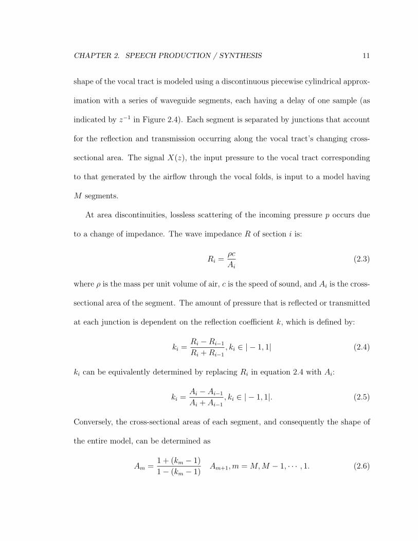
shape of the vocal tract is modeled using a discontinuous piecewise cylindrical approx-
imation with a series of waveguide segments, each having a delay of one sample (as
indicated by z−1 in Figure 2.4). Each segment is separated by junctions that account
for the reflection and transmission occurring along the vocal tract’s changing cross-
sectional area. The signal X(z), the input pressure to the vocal tract corresponding
to that generated by the airflow through the vocal folds, is input to a model having
M segments.
At area discontinuities, lossless scattering of the incoming pressure p occurs due
to a change of impedance. The wave impedance R of section i is:
Ri =ρc
Ai(2.3)
where ρ is the mass per unit volume of air, c is the speed of sound, and Ai is the cross-
sectional area of the segment. The amount of pressure that is reflected or transmitted
at each junction is dependent on the reflection coefficient k, which is defined by:
ki =Ri −Ri−1
Ri + Ri−1, ki ∈ |− 1, 1| (2.4)
ki can be equivalently determined by replacing Ri in equation 2.4 with Ai:
ki =Ai − Ai−1
Ai + Ai−1, ki ∈ |− 1, 1|. (2.5)
Conversely, the cross-sectional areas of each segment, and consequently the shape of
the entire model, can be determined as
Am =1 + (km − 1)
1− (km − 1)Am+1, m = M, M − 1, · · · , 1. (2.6)
CHAPTER 2. SPEECH PRODUCTION / SYNTHESIS 12
Therefore, the reflection coefficient, and the output of the model itself, is largely
dependent on the shape of the vocal tract.
At each junction, the resulting left and right-going pressure waves can be calculated
by the scattering equation:
p+i = (1 + ki)p
+i−1 + kip
−i (2.7)
p−i−1 = kip+i−1 + (1− ki)p
−i (2.8)
where p−i and p+i represent their respective left and right-going pressure at segment
i. The reflection functions at the lips RL(ω) and glottis R0(ω) define the manner in
which pressure is reflected and transmitted at each end of the model. These reflection
functions can be scalar values or filters. The output of this model Y (z) will depend
on the series of recursive interactions, as pressure circulates at each junction.
This model simulates the speech production process and allows further examina-
tion of the vocal tract’s effect on speech. From this model, it becomes possible to
identify k, which can be used (as shown in Equation 2.6) to find the cross-sectional
area for each segment of the model. This study identifies formants produced by the
user and matches these to the output of the model having a similar spectral envelope,
thereby identifying the vocal tract shape of the user that was used to produce the
recorded speech.
Chapter 3
Feature Extraction
3.1 General Features/Background
The development of the proposed study was inspired following a study of existing
methods for feature extraction that are frequently used to characterized the voice.
Independently, these features can all act as an input parameter for musical control.
While many features identify qualities that are directly related to physical phenomena,
like pitch, others are more subjective qualities; for instance, the roughness of the voice.
This study details an assortment of these features to provide background of current
features related to the voice.
13
CHAPTER 3. FEATURE EXTRACTION 14
0 0.1 0.2 0.3 0.4 0.5 0.6 0.7 0.8 0.9 10
500
1000Spectral Centroid
0 0.1 0.2 0.3 0.4 0.5 0.6 0.7 0.8 0.9 10
500Spectral Spread
0 0.1 0.2 0.3 0.4 0.5 0.6 0.7 0.8 0.9 10
0.5
1Spectral Flatness
0 0.1 0.2 0.3 0.4 0.5 0.6 0.7 0.8 0.9 11
0
1
Time (seconds)
"This is a test"
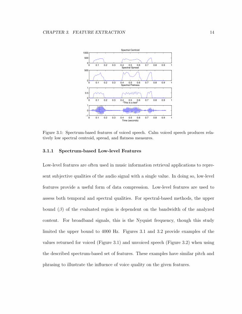
Figure 3.1: Spectrum-based features of voiced speech. Calm voiced speech produces rela-tively low spectral centroid, spread, and flatness measures.
3.1.1 Spectrum-based Low-level Features
Low-level features are often used in music information retrieval applications to repre-
sent subjective qualities of the audio signal with a single value. In doing so, low-level
features provide a useful form of data compression. Low-level features are used to
assess both temporal and spectral qualities. For spectral-based methods, the upper
bound (β) of the evaluated region is dependent on the bandwidth of the analyzed
content. For broadband signals, this is the Nyquist frequency, though this study
limited the upper bound to 4000 Hz. Figures 3.1 and 3.2 provide examples of the
values returned for voiced (Figure 3.1) and unvoiced speech (Figure 3.2) when using
the described spectrum-based set of features. These examples have similar pitch and
phrasing to illustrate the influence of voice quality on the given features.
CHAPTER 3. FEATURE EXTRACTION 15
0 0.2 0.4 0.6 0.8 10
5000Spectral Centroid
0 0.2 0.4 0.6 0.8 10
2000
4000Spectral Spread
0 0.2 0.4 0.6 0.8 10
0.5
1Spectral Flatness
0 0.2 0.4 0.6 0.8 11
0
1"This is a test"
Time (seconds)
Figure 3.2: Spectrum-based features of unvoiced speech. The spectral centroid, spread andflatness values are higher than the voiced speech example due to a more even distributionacross the magnitude spectrum.
The brightness of the voice can be identified by calculating the spectral centroid.
The spectral centroid is known as the center of mass of the power spectrum. It is
calculated as the weighted mean of the frequencies that are present in the signal. The
higher the centroid, the more powerful the higher frequencies are in relation to the
entire spectrum. The centroid can be calculated by:
ψ =
�βk=0 fk|X(k)|2
�βk=0 |X(k)|2
(3.1)
where fk is the frequency (in Hz) of FFT bin k and X(·) is the spectrum of the signal
x(·). Figures 3.1 and 3.2 show that centroid of voiced speech is lower than that of
unvoiced speech, which is likely due to greater emphasis in high-frequency content of
unvoiced speech.
The intensity of the voice can be described by determining the signal’s spectral
CHAPTER 3. FEATURE EXTRACTION 16
spread, defined as the deviation of the spectrum from its mean value. This feature
characterizes how wide significant components to the overall spectrum are. The func-
tion for spectral spread is:
σ =
��βk=0(fk − ψ)2|X(k)|2
�βk=0 |X(k)|2
(3.2)
where ψ is the spectral centroid given in Equation 3.1. Signals with a narrower
bandwidth, like a calm voice, will have a lower spectral spread, whereas broadband
sounds, like a raspy voice, will be higher. Like the centroid, the spectral spread of
unvoiced speech in Figure 3.2 is higher than the voiced speech example (Figure 3.1).
The two figures also show that the spectral centroid and spectral spread are strongly
related, though not identical, when measuring the voice in this manner.
To quantify the level of noise relative to the tonal portion of the sound, the spectral
flatness may be measured by calculating the ratio of the geometric mean and the
arithmetic mean for subdivided portions of the power spectrum:
αb =
Nb
��kb|X(kb)|2
1Nb
�kb|X(kb)|2
(3.3)
kb is from the lower (kl) to upper (ku) edge of the band, while Nb = ku − kl + 1. The
spectral flatness measure is the mean of the sub-band flatness calculations αb, which
returns a value between 0 and 1. This measure is a useful tool for determining whether
speech is pitched or noise [8], where pitched speech will have a lower spectral flatness
measure. Figures 3.1 and 3.2 show the spectrum of speech is flatter when producing
unvoiced speech, as the spectra of unvoiced sounds are typically noisier than that of
CHAPTER 3. FEATURE EXTRACTION 17
voiced speech.
3.1.2 Time domain low-level features
Time domain low-level features identify a wide variety of characteristics. Figure 3.3
illustrates measurements obtained calculating the local energy, temporal centroid,
and zero crossing measure of voiced speech. The local energy of an input signal can
be a crude estimate for the identification voiced/unvoiced, though is more commonly
implemented to identify onsets, as transients have higher energy than the steady state
portion of the signal. The total energy in a signal of N samples is given by:
E(n) =1
N
N2 −1�
m=−N2
|x(n + m)|2w(m) (3.4)
where w(m) is an N -point window centered at m = 0. For improved results, the
time derivative of the energy is observed instead to further exaggerate sudden rises in
energy [2].
The temporal centroid [23] is commonly implemented to distinguish percussive
from sustained sounds. By calculating the temporal centroid, the effective duration
of a sustained tone can be calculated. The centroid is related to the local energy as
it is the time averaged over the energy envelope:
tc =
�t E(t) ∗ t�
t E(t)(3.5)
CHAPTER 3. FEATURE EXTRACTION 18
0 0.1 0.2 0.3 0.4 0.5 0.6 0.7 0.8 0.90
0.02
0.04Local Energy
0 0.1 0.2 0.3 0.4 0.5 0.6 0.7 0.8 0.90
0.5
1Temporal Centroid
0 0.1 0.2 0.3 0.4 0.5 0.6 0.7 0.8 0.90
10
20Zero Crossing
0 0.1 0.2 0.3 0.4 0.5 0.6 0.7 0.8 0.91
0
1"This is a test"
Time (seconds)
Figure 3.3: Time domain features of voiced speech. The local energy provides a smoothedrepresentation of the amplitude envelope, while a high temporal centroid value correspondsto a sustained tone.
where t corresponds to time in samples of the frame and E is calculated from Equa-
tion 3.4. This measure identifies when and how long a sustained sound is percep-
tually meaningful. As the middle plot of Figure 3.3 illustrates, the word “this” is
sustained much longer than “is a test”, thereby producing a significantly higher tem-
poral centroid value which signifies the presence of a sustained tone. Sustained tones
are commonly approximated by identifying when the energy envelop exceeds a given
threshold. While this threshold can vary, a general value of 40% is normally used [23].
Another low-level feature is pitch. The pitch of a speech signal is a function of
the excitation signal generated by the glottis. One of the most common time domain
techniques to estimate pitch is to identify the period from the signals autocorrelation
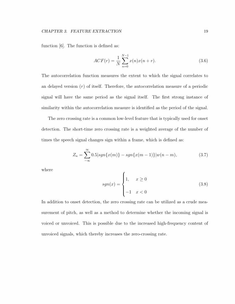
CHAPTER 3. FEATURE EXTRACTION 19
function [6]. The function is defined as:
ACF (r) =1
N
N−1�
n=0
x(n)x(n + r). (3.6)
The autocorrelation function measures the extent to which the signal correlates to
an delayed version (r) of itself. Therefore, the autocorrelation measure of a periodic
signal will have the same period as the signal itself. The first strong instance of
similarity within the autocorrelation measure is identified as the period of the signal.
The zero crossing rate is a common low-level feature that is typically used for onset
detection. The short-time zero crossing rate is a weighted average of the number of
times the speech signal changes sign within a frame, which is defined as:
Zn =∞�
−∞0.5|sgn{x(m)}− sgn{x(m− 1)}|w(n−m), (3.7)
where
sgn(x) =
1, x ≥ 0
−1 x < 0
(3.8)
In addition to onset detection, the zero crossing rate can be utilized as a crude mea-
surement of pitch, as well as a method to determine whether the incoming signal is
voiced or unvoiced. This is possible due to the increased high-frequency content of
unvoiced signals, which thereby increases the zero-crossing rate.
CHAPTER 3. FEATURE EXTRACTION 20
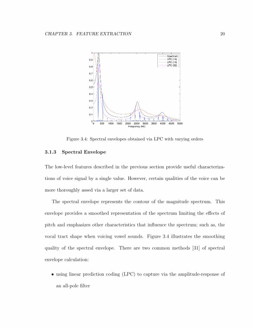
Figure 3.4: Spectral envelopes obtained via LPC with varying orders
3.1.3 Spectral Envelope
The low-level features described in the previous section provide useful characteriza-
tions of voice signal by a single value. However, certain qualities of the voice can be
more thoroughly assed via a larger set of data.
The spectral envelope represents the contour of the magnitude spectrum. This
envelope provides a smoothed representation of the spectrum limiting the effects of
pitch and emphasizes other characteristics that influence the spectrum; such as, the
vocal tract shape when voicing vowel sounds. Figure 3.4 illustrates the smoothing
quality of the spectral envelope. There are two common methods [31] of spectral
envelope calculation:
• using linear prediction coding (LPC) to capture via the amplitude-response of
an all-pole filter
CHAPTER 3. FEATURE EXTRACTION 21
• cepstral windowing to lowpass-filter the log-magnitude spectrum
As the name implies, LPC coefficients are acquired from a linear combination of
previous samples:
x(n) = x(n) =p�
k=1
akx(n− k) (3.9)
where p is the order of the filter and ak is the kth coefficient. LPC aims to match the
filter that generated previous samples of the analyzed signal.
This approximation based on the previous samples will likely not be exact, which
leads to an error (residual) signal:
ε(n) = x(n)− x(n) = x(n)−p�
k=1
akx(n− k) (3.10)
The objective is to find the optimal set of coefficients that minimizes the short-term
energy of the residual:
E =�
m
ε2(n) =�
n
(x(n)−p�
k=1
akx(n− k))2. (3.11)
By minimizing the short-term energy, LPC filter coefficients correspond to a time-
invariant filter that best approximates the analyzed region. When considering source-
filter and waveguide models (described in Chapter 2), the filter of a speech signal
corresponds to the vocal tract. Therefore, the coefficients derived from LPC directly
correspond to the effects the vocal tract has on the spectrum of a signal. Based on
this, the frequency response of these coefficients show the spectral envelope of the
vocal tract filter.
CHAPTER 3. FEATURE EXTRACTION 22
One method that finds this optimal coefficient set is Levinson-Durbin recursion,
which is defined as:
E(0) = R(0)
ki =R(i)−
�i−1j=1 a(i−1)
j R(i− j)
E(i−1), 1 ≤ i ≤ p
a(i)i = ki
a(i)j = a(i−1)
j − kia(i−1)(i−j), 1 ≤ j ≤ i− 1
E(i) = (1− k2i )E(i− 1) (3.12)
where R is the autocorrelation function described in Equation 3.6 and ki corresponds
to the partial correlation coefficients. The final solution is aj = apj for 1 ≤ j ≤ p. The
amplitude response of these all-pole coefficients yields the spectral envelope.
As shown in Figure 3.4, the resonant regions of the spectral envelope are centered
around a peak. These peaks are defined as formants, which denote the resonant
frequencies generated via a particular vocal tract shape. The position of the formants
can be derived by calculating the poles of the linear prediction coefficients.
The order of the LPC filter impacts the accuracy of the spectral envelope, though
the precise order for a given signal is difficult to correctly obtain [35]. In a general
sense, the higher the order, the more detailed the spectral envelope, however increasing
the order also increases the complexity of the procedure. Figure 3.4 illustrates how
the spectral envelope increases in detail when the order is increased. This study used
an order of 22.

CHAPTER 3. FEATURE EXTRACTION 23
As mentioned previously, spectral envelopes can also be calculated using cepstrum
coefficients [25]. When using a comparable order to LPC, similar spectral envelopes
can be obtained. The cepstrum is the result of taking the Fourier Transform of the log
spectrum as if it were the incoming signal. The most common usage of the cepstrum
is in Mel-frequency cepstrum coefficients, which are typically used to measure the
rate of change in logarithmically spaced spectral bands in order to mimic the human
auditory system’s perception of sound. If we define X(k) to represent the K-point
DFT of the signal frame x(n) the cepstrum is calculated by:
C(l) =K�
k=0
log(|X(k)|)ei 2πklK (3.13)
By setting all high frequency elements to 0, the cepstrum becomes a smoothed version
of the amplitude spectrum after taking the Fourier Transform of it. Ultimately, this
approximation is merely an envelop that is based on the mean of the spectrum. The
approximation of the spectral envelope can be improved defining the cepstrum pa-
rameters (notably where zeroing occurs) relative to the fundamental frequency of the
signal, though adding this type of analysis makes the cepstrum analysis undesirable
for real-time performance, especially when there is no guarantee that the parameters
will be optimal during analysis.
Both of the methods provide similarly reasonable results based on the spectrum.
With accurate parameters via fundamental identification, studies [25, 35] have found
that cepstrum based spectral envelopes yield more accurate results compared to lin-
ear prediction with a comparable number of coefficients. However, [25] found that
CHAPTER 3. FEATURE EXTRACTION 24
based vocal tract area function estimation algorithm, specif-ically designed for real-time musical control. As describedin Section 3, the algorithm identifies formants on a sampleframe basis, and places them into streams, enabling theirmovement to be tracked over time.In Section 4, minimum action is applied to improve us-
ability, algorithm performance, and the visual feedback tothe user, by smoothing formant streams to account for un-intended action such as dropped formants or the waveringof an untrained voice (see Section 4). It considers that someusers will have greater control of their voice than others, andprovides a parameter for adjusting the algorithm’s sensitiv-ity to a change in the produced sound.Section 5 describes how estimated formants are com-
pared and matched to a database of formants collected of-fline from the output of the vocal tract model (described inSection 2) having various configurations of cross-sectionalarea.
2 A SIMPLIFIED VOCAL TRACT MODEL
It is well known that digital waveguide modeling may beused to simulate plane and spherical waves propagating incylindrical and conical acoustic tubes [16]. More complexshapes, such as those produced by the vocal tract when us-ing the velum, jaw, tongue and lips to voice different vowelsounds, can be approximated using a sequence of cylindri-cal waveguide elements separated by scattering junctionsaccounting for the reflection and transmission that occurswhen a change in cross-sectional area creates a correspond-ing change of impedance.
z−1
z−1
z−1
z−1
p+1 p+
2
p−1 p−2
1 + k
1− k
−k
X(z)
RL(ω)
Y (z)
bR0(ω) k
Figure 1. A waveguide model of an acoustic tube closedat one end with reflection R0(ω) and open at the other withreflection RL(ω). The tube has a single change in cross-sectional area at the center, creating a two-port scatteringjunction with reflection and transmission defined by k, a co-efficient set according to the relative areas of the two sec-tions.
The way in which a shape departing from the purely cylin-drical contributes to formant peaks in the magnitude spec-trum may be seen by considering a simple model with onlytwo cylindrical waveguide segments of the same length butwith different cross-sectional areas, A1 and A2 respectively(see Figure 1). The two-port scattering junction modelsthe reflection and transmission that occurs at the change incross-sectional area, where the reflection coefficient is given
byk = (A1 −A2)/(A1 + A2). (1)
The response at Y (z) (corresponding to the mouth) to inputX(z) (corresponding to the glottis) is given by
Y (z) = X(z)(1 + k)z−2[1 + b + b2 + . . .] +Y (z)RL(z)R0(z)(1− k2)z−4[1 + b + . . .] +Y (z)RL(−k)z−2, (2)
whereb = R0(z)kz−2. (3)
Equation (2) is the sum of three terms corresponding to thepossible signal flow paths to Y (z), with the first two termsincluding the infinite series generated by the circulating pathin the first waveguide segment (which may be represented inclosed form). Further substituting (3) into (2) yields all-polefilter transfer function
H(z) = Y (z)/X(z)
=(1 + k)z−2
1 + k(RL(z)−R0(z))z−2 −RL(z)R0(z)z−4.
(4)
Setting end reflection functions
R0(z) = 1, and RL(z) = −1
makes the system lossless with transfer function
H(z) =(1 + k)z−2
1 + 2kz−2 + z−4, (5)
preserves the harmonic structure of an open end tube, andallows for observation of the effects of the junction.Factoring the denominator in (5) yields the intermediate
complex conjugate pair,
ρ = k + j�
1− k2 ρ∗ = k − j�
1− k2, (6)
and ultimately the four roots/poles of the filter given by
p1 =√
ρ, p2 = −√ρ, p3 = p∗1, p4 = p∗2. (7)
Figure 2 shows how the poles shift as a function of k andthus in response to a change in cross-sectional area. Shift-ing poles corresponds to a shift of harmonic peaks in themagnitude which, when more sections with varying cross-section are considered, leads to regions in the spectrum withincreased and decreased energy, and the appearance of for-mant peaks during vowel production.Increasing the number of segments increases the number
of poles in the vocal tract transfer function. As shown in(6) and (7), filter poles are a function of the reflection co-efficient, allowing a change in cross-sectional area to be in-ferred direction from filter poles. The complexity involved
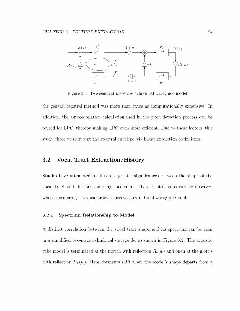
Figure 3.5: Two segment piecewise cylindrical waveguide model
the general cepstral method was more than twice as computationally expensive. In
addition, the autocorrelation calculation used in the pitch detection process can be
reused for LPC, thereby making LPC even more efficient. Due to these factors, this
study chose to represent the spectral envelope via linear prediction coefficients.
3.2 Vocal Tract Extraction/History
Studies have attempted to illustrate greater significances between the shape of the
vocal tract and its corresponding spectrum. These relationships can be observed
when considering the vocal tract a piecewise cylindrical waveguide model.
3.2.1 Spectrum Relationship to Model
A distinct correlation between the vocal tract shape and its spectrum can be seen
in a simplified two-piece cylindrical waveguide, as shown in Figure 3.2. The acoustic
tube model is terminated at the mouth with reflection Ro(w) and open at the glottis
with reflection RL(w). Here, formants shift when the model’s shape departs from a

CHAPTER 3. FEATURE EXTRACTION 25
−1 −0.5 0 0.5 1
−1
−0.8
−0.6
−0.4
−0.2
0
0.2
0.4
0.6
0.8
1
Real Part
Imag
inar
y Pa
rt
k = 0 (uniform tube)
k = 0.8, An = [0.1 1]
k = −0.8, An = [1 0.1]
k = 0.33, An = [0.5 1]
k = −0.33, An = [1 0.5]
Figure 2. The four poles of transfer function (5) plotted forfive values of reflection coefficient k. The uniform cylin-drical tube has a reflection coefficient of k = 0 and corre-sponds to a uniform/harmonic spacing of poles (or peaks inthe magnitude spectrum). A change in k corresponds to achange in the cross-sectional area to the tube and the ob-served shifting of poles in the vocal tract transfer function.
in this recursive problem however, is unnecessarily expen-sive (though not prohibitively so) for real-time applications,and yields far more data than is required to identify the vo-cal tract shape with the accuracy desired here. Rather, it wasfound that a vocal tract shape could be sufficiently charac-terized using only up four formant peaks in the magnitudeof its frequency response.
3 TRACKING FORMANTS IN VOCAL OUTPUT
0 500 1000 1500 2000 2500 3000 3500 4000−1
−0.8
−0.6
−0.4
−0.2
0
0.2
0.4
0.6
0.8
1
Frequency (Hz)
Nor
mal
ized
Am
plitu
de
Log Spectrum and Second Derivative
Log SpectrumSecond DerivativePeak ID
Figure 3. The log magnitude spectrum of an input sam-ple frame (upper solid line) and its second derivative (lowerbroken line), with the latter accentuating the position of“merged” formants.
An incoming sample frame of recorded voice is win-dowed and processed to extract its spectral envelope—a curveassumed to approximate the magnitude of the vocal tract fre-quency response—with formants peaks in the spectra beingidentified by tracking curve local maxima.Notice from the log spectrum in Figure 3 (upper curve)
that the position of weaker formants is sometimes obscuredby the presence of more pronounced formants having greateramplitude and bandwidth. As shown by the broken-linecurve in Figure 3 (lower curve), the second derivative ofthe log magnitude spectrum may be taken to produce moreprominent bends in the curve contour at peak locations, ef-fectively reducing the formant bandwidth and accentuatingthe position of “merged” formants [13]. Though is also pos-sible to take the third derivative of the phase spectrum [8]to yield further improvement in bandwidth attenuation andpeak accentuation, this method was found to be less success-ful in tracking merged formants with significantly differentamplitudes, and thus produced less consistent results.Once the most prominent formant peaks are detected,
they are placed into formant streams that track the move-ment of a formant number from frame to frame. These for-mant streams are necessary to account for dropped formantsand improve usability and performance as discussed in Sec-tion 4. Limiting the streams to a maximum of four was suffi-cient to uniquely identify a corresponding vocal tract model.
Figure 4. Example of formant stream assignment: Analysisof current frame Fn yields two detected formant peaks at154 Hz and 2492 Hz. The first peak at 154 Hz is closest tothe first formant of the previous frame Fn−1 and is thus as-signed to the first formant stream f1(n). Similarly, the peakat 2492 Hz is assigned to the third formant stream f3(n).To accommodate for the “dropped” formant in the secondstream, the last value assigned from the previous frame isheld over to the current frame.
To determine to which stream a formant peak should beassigned, a distance measure is taken between the estimatedformant peak of a current frame Fn and the stream-assignedneighbouring formants of the previous frame, Fn−1, withthe formant being assigned to the stream of its neighbourclosest in frequency. If the difference between formant fre-
Figure 3.6: Pole location relative to reflection coefficient
purely cylindrical tube, where k > 0. When k is altered by adjusting the change in
cross-sectional areas, the formants shift in the magnitude spectrum.
A recent study [18] demonstrated the unique relationship between formant location
and the vocal tract shape, as formant locations were shown to be calculated directly
based on the reflection coefficient. When considering all possible signal pathways
to the mouth (Y (z)) based on the two-segment waveguide shown in Figure 3.2, the
response of Y (z) to input X(z) (corresponding to the glottis) is given by
Y (z) =X(z)(1 + k)z−2[1 + b + b2 + ...]+
Y (z)RL(z)R0(z)(1− k2)z−4[1 + b + ...]+
Y (z)RL(−k)z−2 (3.14)
where
b = R0(z)kz−2. (3.15)
CHAPTER 3. FEATURE EXTRACTION 26
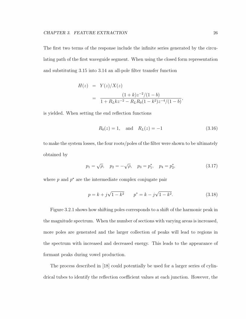
The first two terms of the response include the infinite series generated by the circu-
lating path of the first waveguide segment. When using the closed form representation
and substituting 3.15 into 3.14 an all-pole filter transfer function
H(z) = Y (z)/X(z)
=(1 + k)z−2/(1− b)
1 + RLkz−2 −RLR0(1− k2)z−4/(1− b),
is yielded. When setting the end reflection functions
R0(z) = 1, and RL(z) = −1 (3.16)
to make the system losses, the four roots/poles of the filter were shown to be ultimately
obtained by
p1 =√
ρ, p2 = −√ρ, p3 = p∗1, p4 = p∗2, (3.17)
where p and p� are the intermediate complex conjugate pair
p = k + j√
1− k2 p∗ = k − j√
1− k2. (3.18)
Figure 3.2.1 shows how shifting poles corresponds to a shift of the harmonic peak in
the magnitude spectrum. When the number of sections with varying areas is increased,
more poles are generated and the larger collection of peaks will lead to regions in
the spectrum with increased and decreased energy. This leads to the appearance of
formant peaks during vowel production.
The process described in [18] could potentially be used for a larger series of cylin-
drical tubes to identify the reflection coefficient values at each junction. However, the
CHAPTER 3. FEATURE EXTRACTION 27
complexity involved for this recursive problem is prohibitively expensive for real-time
applications and yields substantially more data than is required to identify the vocal
tract shape with the accuracy needed for the intended application of this study.
3.2.2 Previous Vocal Tract Shape Estimation Methods
Studies [36, 37] determined that with certain conditions, the recursive relation of
finding the optimal inverse filter through LPC or autoregressive (AR) models using
Yule-Walker or Levinson-Durbin methods is identical to the recursive nature of the
acoustic tube model. Therefore, the reflection coefficients of the model can be obtained
when recursively calculating the filter coefficients. Since the reflection coefficients are
directly related to the change in cross sectional area of each segment of the model,
[36] states that the shape of the vocal tract can be retrieved from the speech signal.
The observations made in [36] are based on various assumptions of the model:
• The cross-sectional area of each segment is small enough to treat the propagating
wave as a plane wave.
• Propagation loses due to viscosity and heat conduction are negligible.
• The reflection coefficient of the lips is assumed to be -1.
• The reflection coefficient of the glottis is an arbitrary value between 0 and 1.
• The glottal source exhibits a flat frequency response.
CHAPTER 3. FEATURE EXTRACTION 28
1 2 3 4 5 6 7
Original
1 2 3 4 5 6 7
Original
1 2 3 4 5 6 7
Estimated
Segments1 2 3 4 5 6 7
Estimated
Segments
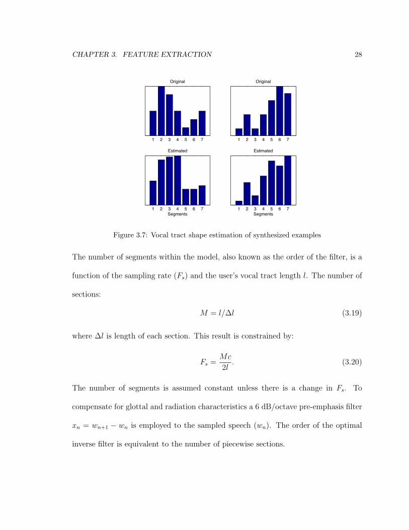
Figure 3.7: Vocal tract shape estimation of synthesized examples
The number of segments within the model, also known as the order of the filter, is a
function of the sampling rate (Fs) and the user’s vocal tract length l. The number of
sections:
M = l/∆l (3.19)
where ∆l is length of each section. This result is constrained by:
Fs =Mc
2l. (3.20)
The number of segments is assumed constant unless there is a change in Fs. To
compensate for glottal and radiation characteristics a 6 dB/octave pre-emphasis filter
xn = wn+1 − wn is employed to the sampled speech (wn). The order of the optimal
inverse filter is equivalent to the number of piecewise sections.
CHAPTER 3. FEATURE EXTRACTION 29
To obtain the vocal tract shape using this recursive technique, the reflection coef-
ficient of segment i relates to the previous iteration of recursion (ki). At step one, the
reflection coefficient corresponding to the junction closest to the lips is k0 = −r1/r0,
which is a result of the second step of Equation 3.12 within the Levinson-Durbin re-
cursion process. Similarly, the final reflection coefficient equals kM−1, which is derived
from ?? and the aMi are computed from kM−1 and aM−1
i by use of ??/??.
The cross-sectional area for each section can be computed from the reflection
coefficients through equation 2.6. Based on the relational manner of the equation,
AM is obtained by specifying AM+1 = 1.
3.2.3 Motivation for New Approach
Despite its usage in more current studies [21, 29], many have noted that the estimation
of the vocal tract shape from reflection coefficients have produced inconsistent and
inaccurate results due to a variety of limitations. Estimations based on a LPC models
are derived by assuming a flat glottal pulse spectrum [31]. Some [22, 37] have found
that the filter which aims to neutralize the effects of the glottal pulse and lip radiation
characteristics in order to flatten the glottal pulse spectrum are insufficient. These
studies also identify the unspecified termination reflection/transmission functions and
propagation losses as inaccuracy factors.
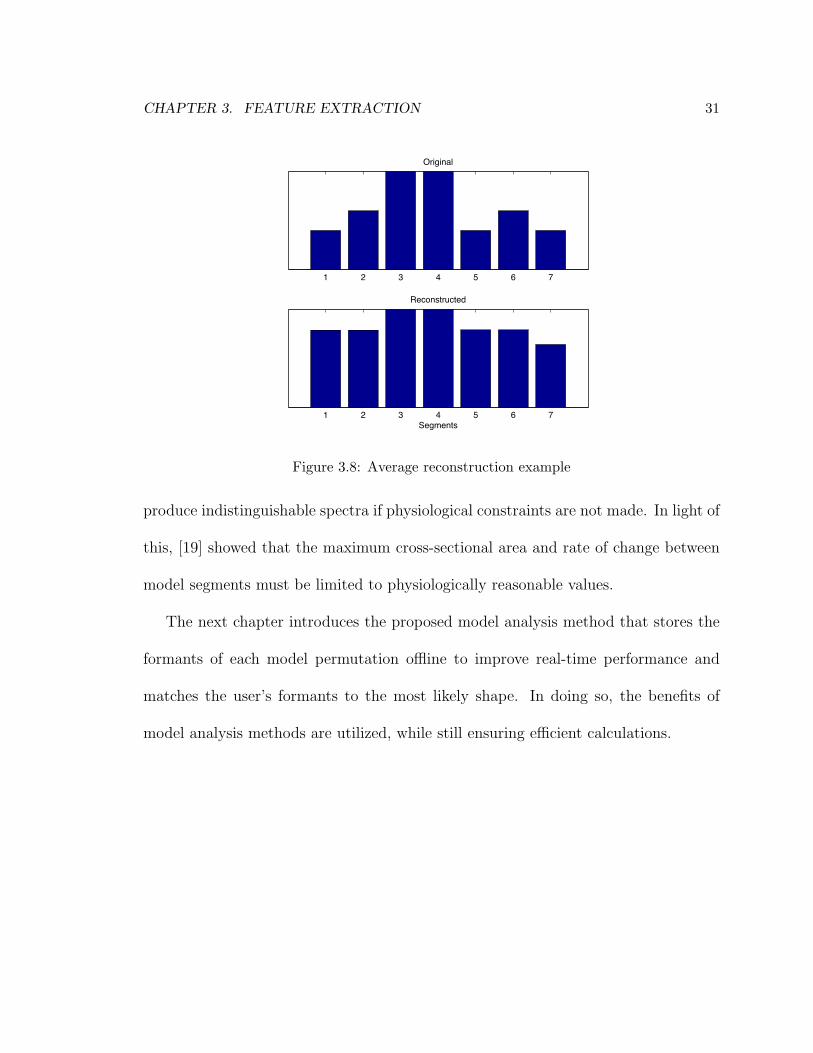
In general practice, this study found the algorithm to be rather inconsistent when
CHAPTER 3. FEATURE EXTRACTION 30
running simplified examples. Figure 3.3 shows the estimated shapes of synthesized vo-
cal tracts, which use the same boundary conditions given in [36]. To further illustrate
the inaccuracy of [36], the shapes of 15, 625 unique, seven-segment digital waveguide
models were estimated using Wakita’s method. The estimated shapes were then com-
pared to actual in order to identify how closely the estimation was to the actual shape.
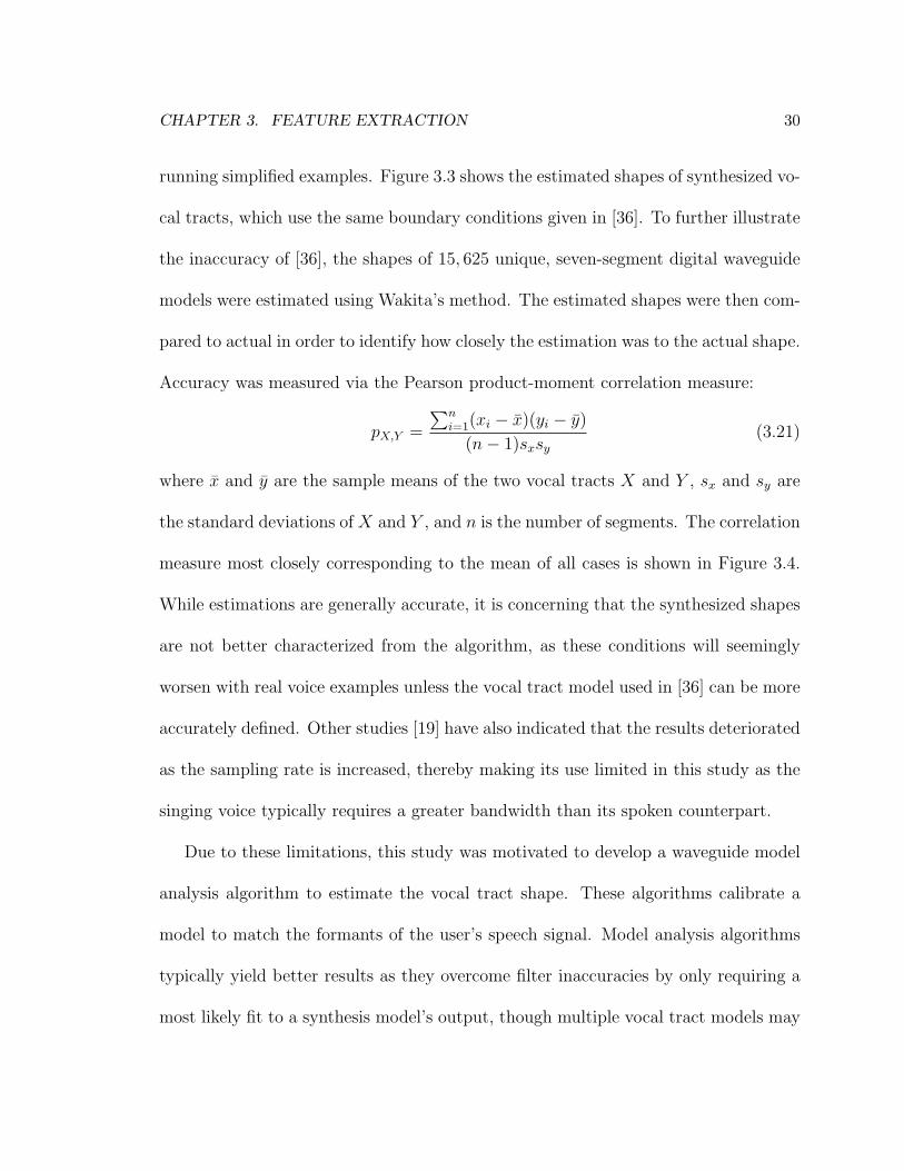
Accuracy was measured via the Pearson product-moment correlation measure:
pX,Y =
�ni=1(xi − x)(yi − y)
(n− 1)sxsy(3.21)
where x and y are the sample means of the two vocal tracts X and Y , sx and sy are
the standard deviations of X and Y , and n is the number of segments. The correlation
measure most closely corresponding to the mean of all cases is shown in Figure 3.4.
While estimations are generally accurate, it is concerning that the synthesized shapes
are not better characterized from the algorithm, as these conditions will seemingly
worsen with real voice examples unless the vocal tract model used in [36] can be more
accurately defined. Other studies [19] have also indicated that the results deteriorated
as the sampling rate is increased, thereby making its use limited in this study as the
singing voice typically requires a greater bandwidth than its spoken counterpart.
Due to these limitations, this study was motivated to develop a waveguide model
analysis algorithm to estimate the vocal tract shape. These algorithms calibrate a
model to match the formants of the user’s speech signal. Model analysis algorithms
typically yield better results as they overcome filter inaccuracies by only requiring a
most likely fit to a synthesis model’s output, though multiple vocal tract models may
CHAPTER 3. FEATURE EXTRACTION 31
1 2 3 4 5 6 7
Original
1 2 3 4 5 6 7
Reconstructed
Segments
Figure 3.8: Average reconstruction example
produce indistinguishable spectra if physiological constraints are not made. In light of
this, [19] showed that the maximum cross-sectional area and rate of change between
model segments must be limited to physiologically reasonable values.
The next chapter introduces the proposed model analysis method that stores the
formants of each model permutation offline to improve real-time performance and
matches the user’s formants to the most likely shape. In doing so, the benefits of
model analysis methods are utilized, while still ensuring efficient calculations.
Chapter 4
Estimation of Vocal Tract Shape
The features described in Chapter 3 illustrate ways to characterize qualities of the
voice in a compressed form and showed how certain features, particularly formants,
relate to the vocal tract shape. This chapter describes an algorithm that matches the
user’s formants to the most similar set of formants generated by a particular waveguide
model shape. To compensate for users of all abilities, this algorithm incorporates a
scheme that provides reliable feedback in spite of inconstant performance. The scheme
is as follows:
• Detect a voice onset to initiate the procedure.
• Extract formants from the user using the second derivative of the log spectrum.
• Place the formant into the appropriate “stream” to track change over time.
• Smooth the stream to improve feedback by averaging past frames.
32
CHAPTER 4. ESTIMATION OF VOCAL TRACT SHAPE 33
• Match a model shape to the user’s formant set.
• Transition between old and new vocal tract shapes.
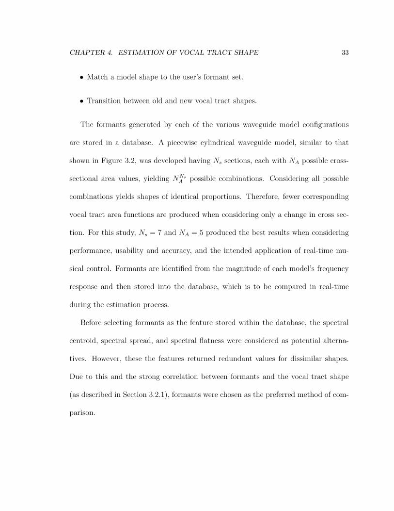
The formants generated by each of the various waveguide model configurations
are stored in a database. A piecewise cylindrical waveguide model, similar to that
shown in Figure 3.2, was developed having Ns sections, each with NA possible cross-
sectional area values, yielding NNsA possible combinations. Considering all possible
combinations yields shapes of identical proportions. Therefore, fewer corresponding
vocal tract area functions are produced when considering only a change in cross sec-
tion. For this study, Ns = 7 and NA = 5 produced the best results when considering
performance, usability and accuracy, and the intended application of real-time mu-
sical control. Formants are identified from the magnitude of each model’s frequency
response and then stored into the database, which is to be compared in real-time
during the estimation process.
Before selecting formants as the feature stored within the database, the spectral
centroid, spectral spread, and spectral flatness were considered as potential alterna-
tives. However, these the features returned redundant values for dissimilar shapes.
Due to this and the strong correlation between formants and the vocal tract shape
(as described in Section 3.2.1), formants were chosen as the preferred method of com-
parison.
CHAPTER 4. ESTIMATION OF VOCAL TRACT SHAPE 34
−1 −0.5 0 0.5 1
−1
−0.8
−0.6
−0.4
−0.2
0
0.2
0.4
0.6
0.8
1
Real Part
Imag
inar
y Pa
rt
k = 0 (uniform tube)
k = 0.8, An = [0.1 1]
k = −0.8, An = [1 0.1]
k = 0.33, An = [0.5 1]
k = −0.33, An = [1 0.5]
Figure 2. The four poles of transfer function (5) plotted forfive values of reflection coefficient k. The uniform cylin-drical tube has a reflection coefficient of k = 0 and corre-sponds to a uniform/harmonic spacing of poles (or peaks inthe magnitude spectrum). A change in k corresponds to achange in the cross-sectional area to the tube and the ob-served shifting of poles in the vocal tract transfer function.
in this recursive problem however, is unnecessarily expen-sive (though not prohibitively so) for real-time applications,and yields far more data than is required to identify the vo-cal tract shape with the accuracy desired here. Rather, it wasfound that a vocal tract shape could be sufficiently charac-terized using only up four formant peaks in the magnitudeof its frequency response.
3 TRACKING FORMANTS IN VOCAL OUTPUT
0 500 1000 1500 2000 2500 3000 3500 4000−1
−0.8
−0.6
−0.4
−0.2
0
0.2
0.4
0.6
0.8
1
Frequency (Hz)
Nor
mal
ized
Am
plitu
de
Log Spectrum and Second Derivative
Log SpectrumSecond DerivativePeak ID
Figure 3. The log magnitude spectrum of an input sam-ple frame (upper solid line) and its second derivative (lowerbroken line), with the latter accentuating the position of“merged” formants.
An incoming sample frame of recorded voice is win-dowed and processed to extract its spectral envelope—a curveassumed to approximate the magnitude of the vocal tract fre-quency response—with formants peaks in the spectra beingidentified by tracking curve local maxima.Notice from the log spectrum in Figure 3 (upper curve)
that the position of weaker formants is sometimes obscuredby the presence of more pronounced formants having greateramplitude and bandwidth. As shown by the broken-linecurve in Figure 3 (lower curve), the second derivative ofthe log magnitude spectrum may be taken to produce moreprominent bends in the curve contour at peak locations, ef-fectively reducing the formant bandwidth and accentuatingthe position of “merged” formants [13]. Though is also pos-sible to take the third derivative of the phase spectrum [8]to yield further improvement in bandwidth attenuation andpeak accentuation, this method was found to be less success-ful in tracking merged formants with significantly differentamplitudes, and thus produced less consistent results.Once the most prominent formant peaks are detected,
they are placed into formant streams that track the move-ment of a formant number from frame to frame. These for-mant streams are necessary to account for dropped formantsand improve usability and performance as discussed in Sec-tion 4. Limiting the streams to a maximum of four was suffi-cient to uniquely identify a corresponding vocal tract model.
Figure 4. Example of formant stream assignment: Analysisof current frame Fn yields two detected formant peaks at154 Hz and 2492 Hz. The first peak at 154 Hz is closest tothe first formant of the previous frame Fn!1 and is thus as-signed to the first formant stream f1(n). Similarly, the peakat 2492 Hz is assigned to the third formant stream f3(n).To accommodate for the “dropped” formant in the secondstream, the last value assigned from the previous frame isheld over to the current frame.
To determine to which stream a formant peak should beassigned, a distance measure is taken between the estimatedformant peak of a current frame Fn and the stream-assignedneighbouring formants of the previous frame, Fn!1, withthe formant being assigned to the stream of its neighbourclosest in frequency. If the difference between formant fre-
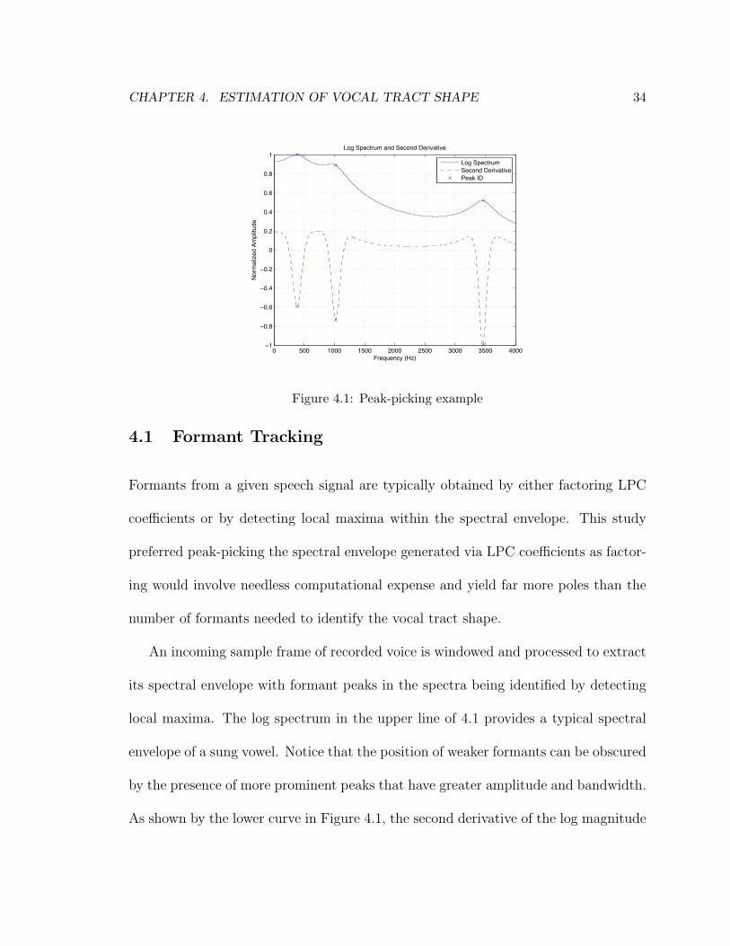
Figure 4.1: Peak-picking example
4.1 Formant Tracking
Formants from a given speech signal are typically obtained by either factoring LPC
coefficients or by detecting local maxima within the spectral envelope. This study
preferred peak-picking the spectral envelope generated via LPC coefficients as factor-
ing would involve needless computational expense and yield far more poles than the
number of formants needed to identify the vocal tract shape.
An incoming sample frame of recorded voice is windowed and processed to extract
its spectral envelope with formant peaks in the spectra being identified by detecting
local maxima. The log spectrum in the upper line of 4.1 provides a typical spectral
envelope of a sung vowel. Notice that the position of weaker formants can be obscured
by the presence of more prominent peaks that have greater amplitude and bandwidth.
As shown by the lower curve in Figure 4.1, the second derivative of the log magnitude
CHAPTER 4. ESTIMATION OF VOCAL TRACT SHAPE 35
spectrum can accentuate less prominent bends in the curve contour and attenuate
the formant bandwidth to reduce this “merging” that can occur when formants are
close in proximity [4]. It is also possible to take the third derivative of the phase
spectrum [17] to further reduce the bandwidth of each formant, however this method
was found to be less consistent in identifying when the amplitudes of merged formants
were significantly different amplitudes.
4.1.1 Real-Time Considerations
To assist in the database search process and improve usability for users of all abilities,
each identified formant was placed into their appropriate formant “stream”. These
streams provide a means to track the trajectory of a given formant over time in order
to account for error or user instability. While this concept is not an unfamiliar formant
tracking procedure [28], these streams were devised to improve the database search
process (discussed in section 4.3) by accounting for dropped formants that can occur
over a frame-by-frame basis. There are a maximum of four streams that can be active
at a given time, however it was most common that only three were detected. In
the unlikely event that more than four peaks are identified within a frame, the four
formants of greatest amplitude are placed within the stream. Limiting to a maximum
of four four formants was sufficient to uniquely identify a corresponding vocal tract
model.
CHAPTER 4. ESTIMATION OF VOCAL TRACT SHAPE 36
−1 −0.5 0 0.5 1
−1
−0.8
−0.6
−0.4
−0.2
0
0.2
0.4
0.6
0.8
1
Real PartIm
agin
ary
Part
k = 0 (uniform tube)
k = 0.8, An = [0.1 1]
k = −0.8, An = [1 0.1]
k = 0.33, An = [0.5 1]
k = −0.33, An = [1 0.5]
Figure 2. The four poles of transfer function (5) plotted forfive values of reflection coefficient k. The uniform cylin-drical tube has a reflection coefficient of k = 0 and corre-sponds to a uniform/harmonic spacing of poles (or peaks inthe magnitude spectrum). A change in k corresponds to achange in the cross-sectional area to the tube and the ob-served shifting of poles in the vocal tract transfer function.
in this recursive problem however, is unnecessarily expen-sive (though not prohibitively so) for real-time applications,and yields far more data than is required to identify the vo-cal tract shape with the accuracy desired here. Rather, it wasfound that a vocal tract shape could be sufficiently charac-terized using only up four formant peaks in the magnitudeof its frequency response.
3 TRACKING FORMANTS IN VOCAL OUTPUT
0 500 1000 1500 2000 2500 3000 3500 4000−1
−0.8
−0.6
−0.4
−0.2
0
0.2
0.4
0.6
0.8
1
Frequency (Hz)
Nor
mal
ized
Am
plitu
de
Log Spectrum and Second Derivative
Log SpectrumSecond DerivativePeak ID
Figure 3. The log magnitude spectrum of an input sam-ple frame (upper solid line) and its second derivative (lowerbroken line), with the latter accentuating the position of“merged” formants.
An incoming sample frame of recorded voice is win-dowed and processed to extract its spectral envelope—a curveassumed to approximate the magnitude of the vocal tract fre-quency response—with formants peaks in the spectra beingidentified by tracking curve local maxima.Notice from the log spectrum in Figure 3 (upper curve)
that the position of weaker formants is sometimes obscuredby the presence of more pronounced formants having greateramplitude and bandwidth. As shown by the broken-linecurve in Figure 3 (lower curve), the second derivative ofthe log magnitude spectrum may be taken to produce moreprominent bends in the curve contour at peak locations, ef-fectively reducing the formant bandwidth and accentuatingthe position of “merged” formants [13]. Though is also pos-sible to take the third derivative of the phase spectrum [8]to yield further improvement in bandwidth attenuation andpeak accentuation, this method was found to be less success-ful in tracking merged formants with significantly differentamplitudes, and thus produced less consistent results.Once the most prominent formant peaks are detected,
they are placed into formant streams that track the move-ment of a formant number from frame to frame. These for-mant streams are necessary to account for dropped formantsand improve usability and performance as discussed in Sec-tion 4. Limiting the streams to a maximum of four was suffi-cient to uniquely identify a corresponding vocal tract model.
Figure 4. Example of formant stream assignment: Analysisof current frame Fn yields two detected formant peaks at154 Hz and 2492 Hz. The first peak at 154 Hz is closest tothe first formant of the previous frame Fn!1 and is thus as-signed to the first formant stream f1(n). Similarly, the peakat 2492 Hz is assigned to the third formant stream f3(n).To accommodate for the “dropped” formant in the secondstream, the last value assigned from the previous frame isheld over to the current frame.
To determine to which stream a formant peak should beassigned, a distance measure is taken between the estimatedformant peak of a current frame Fn and the stream-assignedneighbouring formants of the previous frame, Fn!1, withthe formant being assigned to the stream of its neighbourclosest in frequency. If the difference between formant fre-
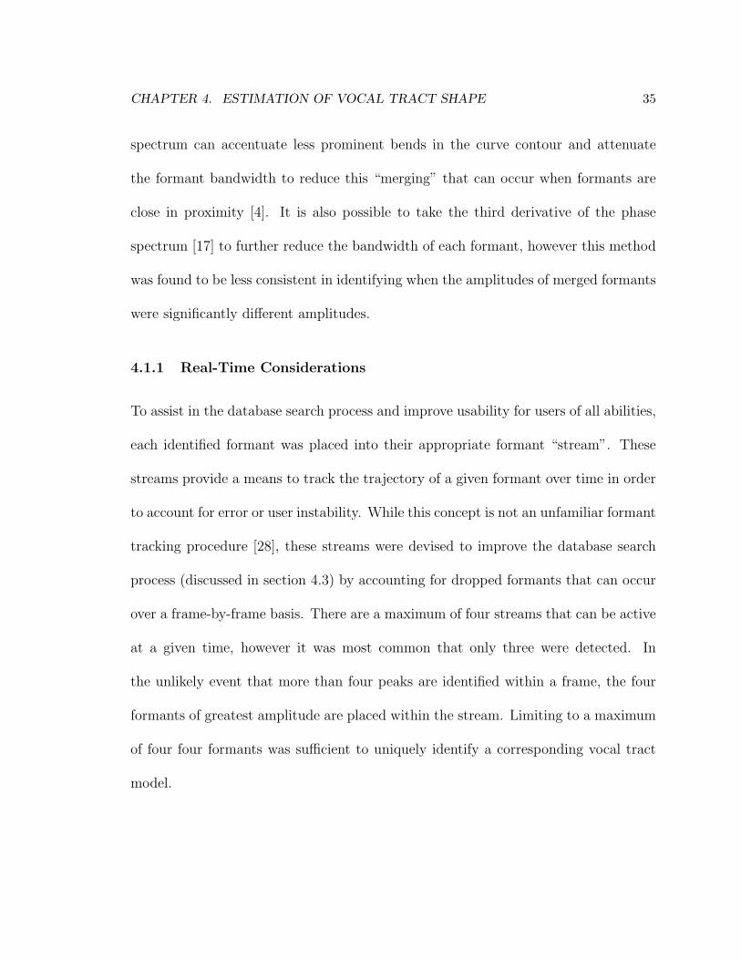
Figure 4.2: Stream selection example
Once the most prominent peaks are detected, they are placed into their appro-
priate stream. The estimated formant peak of the current frame Fn is compared
to the stream-assigned neighboring formants of the previous frame, Fn−1, with the
formant being assigned to the stream of its neighbor closest in frequency. If the dif-
ference between the current formant and its two candidate streams exceeds a specified
threshold, an additional formant stream becomes active. A new stream is started if
multiple current formants differ greatly from frame F(n− 1).
This process is further illustrated by the example in 4.2. The detected 154 Hz
formant of frame Fn is closest to the first formant of the previous frame Fn−1 and is
therefore placed into formant stream f1(n). Similarly, the 2492 Hz formant peaks is
assigned to the third formant stream f3(n). Here only two peaks have been detected in
the current frame despite the three active streams in frame F(n− 1), thereby flagging
the possibility that a formant was unintentionally dropped in frame Fn.
CHAPTER 4. ESTIMATION OF VOCAL TRACT SHAPE 37
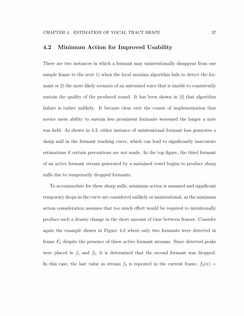
4.2 Minimum Action for Improved Usability
There are two instances in which a formant may unintentionally disappear from one
sample frame to the next 1) when the local maxima algorithm fails to detect the for-
mant or 2) the more likely scenario of an untrained voice that is unable to consistently
sustain the quality of the produced sound. It has been shown in [4] that algorithm
failure is rather unlikely. It became clear over the course of implementation that
novice users ability to sustain less prominent formants worsened the longer a note
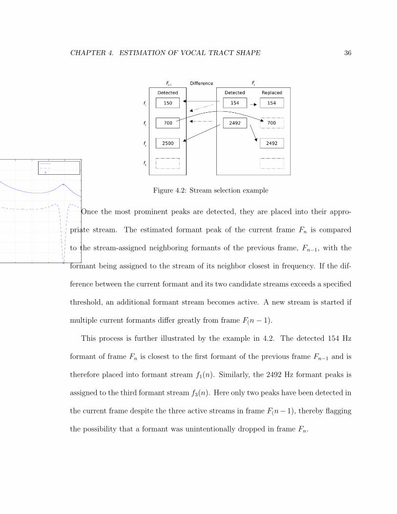
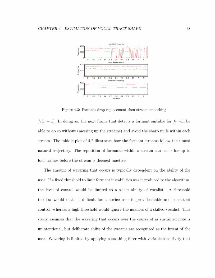
was held. As shown in 4.3, either instance of unintentional formant loss generates a
sharp null in the formant tracking curve, which can lead to significantly inaccurate
estimations if certain precautions are not made. In the top figure, the third formant
of an active formant stream generated by a sustained vowel begins to produce sharp
nulls due to temporarily dropped formants.
To accommodate for these sharp nulls, minimum action is assumed and significant
temporary drops in the curve are considered unlikely or unintentional, as the minimum
action consideration assumes that too much effort would be required to intentionally
produce such a drastic change in the short amount of time between frames. Consider
again the example shown in Figure 4.2 where only two formants were detected in
frame Fn despite the presence of three active formant streams. Since detected peaks
were placed in f1 and f3, it is determined that the second formant was dropped.
In this case, the last value in stream f2 is repeated in the current frame, f2(n) =
CHAPTER 4. ESTIMATION OF VOCAL TRACT SHAPE 38
quencies exceeds a threshold, an additional formant streambecomes active. Though it is possible to have up to fourstreams, it is most common to use only three.The process is illustrated by the example in Figure 4,
where only two peaks have been detected with three activestreams, flagging the possibility that a formant was unin-tentionally “dropped”. Accounting for such absent formantpeaks, as described in Section 4, further improves usabilityof the system.
4 MINIMUM ACTION FOR IMPROVEDUSABILITY
There are the two situations in which a formant may unin-tentionally temporarily disappear from one sample frame tothe next: 1) when the algorithm fails to detect it for a partic-ular frame or more likely 2) an untrained voice is unable toconsistently sustain the quality of the produced sound. Asshown in Figure 5 (top), either instance generates a sharpnull in the formant tracking curve.To accommodate for this, minimum action is assumed,
and such significant temporary drops in the curve are con-sidered unlikely or unintentional (with minimum action sug-gesting too much effort would be required to intentionallyproduce such a drastic change). Consider again the exam-ple shown in Figure 4, which shows only two peaks be-ing detected in the presence of three active formant curves.Since the detected peak is placed in the third stream, it isthe second formant that was dropped. In this case, the lastvalue in the second stream is held over to the current frame,f2(n) = f2(n− 1). In this way, when/if the formant returnsin subsequent frame analysis, it will be placed in the cor-rect stream and the sharp nulls in the curves will be avoided(see top and middle of Figure 5). The repetition of formantswithin a stream can occur up to four times before the streamis deemed inactive.Algorithm performance and visual feedback to the user is
further improved by applying a smoothing filter to the for-mant tracking curves, effectively stabilizing the movementof the formants and compensating for unintentional waver-ing of the less-trained voice. An amplitude envelope fol-lower given by,
fm(n) = (1− ν)|fm(n)| + νfm(n− 1), (8)
is applied to the formant streams fm(n), where ν determineshow quickly changes in fm(n) are tracked. If ν is close toone, changes are tracked slowly, making the smoothed curvefm(n) less sensitive to change. If ν is close to zero, fm(n)has an immediate influence on fm(n). A higher ν, thereforemay be appropriate for untrained voices, but with practice,the parameter value may be decreased to allow for betterdetection of subtle nuances.Regardless of ability, formants shift rapidly during an
onset of (or change in) the vocal/vowel sound, and thus
0.1 0.2 0.3 0.4 0.5 0.6 0.7 0.8 0.9 1 1.10
2000
4000
Freq
uenc
y
Identified formants
0.1 0.2 0.3 0.4 0.5 0.6 0.7 0.8 0.9 1 1.10
2000
4000
Freq
uenc
y
Drop Replacement
0.1 0.2 0.3 0.4 0.5 0.6 0.7 0.8 0.9 1 1.10
2000
4000
Seconds
Freq
uenc
yFormant Smoothing
Figure 5. Three active formant streams with the third streamhaving sharp nulls due to temporarily dropped formants(top). Nulls are avoided by holding values from the pre-vious frame when a formant is flagged as being dropped(middle). Further smoothing is applied to compensate forunintentional wavering in the less-trained voice (bottom).
detected formants are added to streams only once the for-mants have settled and the speech waveform is more sus-tained. (This creates latency in the visual feedback to theuser equal to the onset duration). Extensive methods for de-tecting attacks in sounds from musical instruments are notnecessary here, particularly since they are considered to beless effective when applied to the voice [4]. Figure 6 showsthe waveform recorded when a speaker produces the vowelsounds /ee/ to /oo/ and back to /ee/. In spite of the speaker’sattempt to keep the amplitude constant, the waveform enve-lope clearly shows a change in energy at the locations of thechanging events. This result is expected when consideringthat the waxing and waning in the frequency spectrum dueto shifting formants will have an equivalent effect on the sig-nal’s energy in both time and frequency domains (Parseval’stheorem).The onset of an event is therefore identified solely by
tracking steep slopes in the amplitude envelope of the speechsignal. At an event onset, the formant peaks are still de-tected, but with their rate of change being recorded fromframe to frame. Once this value is sufficiently reduced andthe position of the speaker/singer’s formants settle, the onsetregion is considered to have passed and the algorithm mayresume with the process of formant stream assignment andvocal tract shape estimation.
5 ESTIMATION OF THE VOCAL TRACT SHAPE
With the estimated formant streams in place, the final step isto search the database produced by the output of the modelconfigured to various shapes, and find the most likely can-didate.A piecewise cylindrical waveguide model, similar to that
Figure 4.3: Formant drop replacement then stream smoothing
f2(n − 1). In doing so, the next frame that detects a formant suitable for f2 will be
able to do so without (messing up the streams) and avoid the sharp nulls within each
stream. The middle plot of 4.2 illustrates how the formant streams follow their most
natural trajectory. The repetition of formants within a stream can occur for up to
four frames before the stream is deemed inactive.
The amount of wavering that occurs is typically dependent on the ability of the
user. If a fixed threshold to limit formant instabilities was introduced to the algorithm,
the level of control would be limited to a select ability of vocalist. A threshold
too low would make it difficult for a novice user to provide stable and consistent
control, whereas a high threshold would ignore the nuances of a skilled vocalist. This
study assumes that the wavering that occurs over the course of as sustained note is
unintentional, but deliberate shifts of the streams are recognized as the intent of the
user. Wavering is limited by applying a soothing filter with variable sensitivity that
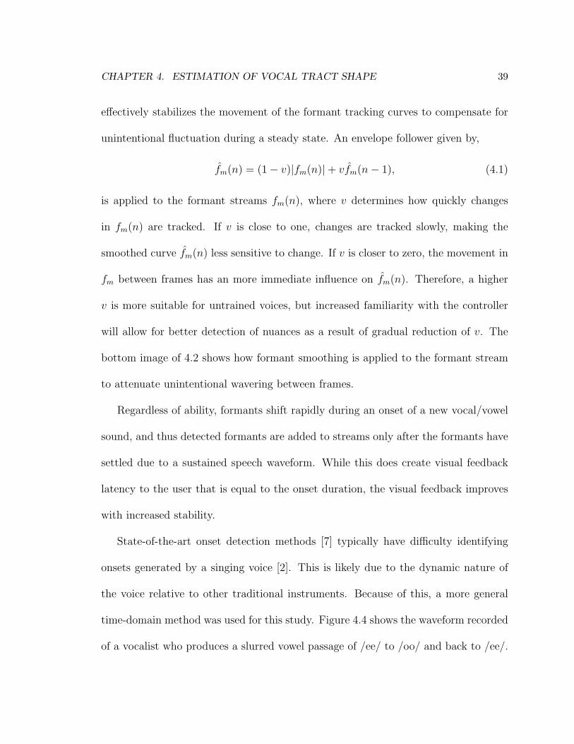
CHAPTER 4. ESTIMATION OF VOCAL TRACT SHAPE 39
effectively stabilizes the movement of the formant tracking curves to compensate for
unintentional fluctuation during a steady state. An envelope follower given by,
fm(n) = (1− v)|fm(n)| + vfm(n− 1), (4.1)
is applied to the formant streams fm(n), where v determines how quickly changes
in fm(n) are tracked. If v is close to one, changes are tracked slowly, making the
smoothed curve fm(n) less sensitive to change. If v is closer to zero, the movement in
fm between frames has an more immediate influence on fm(n). Therefore, a higher
v is more suitable for untrained voices, but increased familiarity with the controller
will allow for better detection of nuances as a result of gradual reduction of v. The
bottom image of 4.2 shows how formant smoothing is applied to the formant stream
to attenuate unintentional wavering between frames.
Regardless of ability, formants shift rapidly during an onset of a new vocal/vowel
sound, and thus detected formants are added to streams only after the formants have
settled due to a sustained speech waveform. While this does create visual feedback
latency to the user that is equal to the onset duration, the visual feedback improves
with increased stability.
State-of-the-art onset detection methods [7] typically have difficulty identifying
onsets generated by a singing voice [2]. This is likely due to the dynamic nature of
the voice relative to other traditional instruments. Because of this, a more general
time-domain method was used for this study. Figure 4.4 shows the waveform recorded
of a vocalist who produces a slurred vowel passage of /ee/ to /oo/ and back to /ee/.

CHAPTER 4. ESTIMATION OF VOCAL TRACT SHAPE 40
0 0.5 1 1.5 2 2.5 3 3.5 40
0.1
0.2
0.3
0.4
0.5
0.6
0.7
0.8
Time (seconds)
Ampl
itude
ee oo ee
Figure 6. Amplitude envelope produced when voicing vow-els /ee/ then /oo/ then back to /ee/ while attempting to keepthe amplitude (loudness) constant. The amplitude envelopeclearly shows the locations of these event changes.
shown in Figure 1, was developed having Ns sections, eachwith NA possible cross-sectional area values, yieldingNNs
Apossible combinations. Considering all possible combina-tions yields duplicate shapes however, fewer correspondingvocal tract area functions are produced by considering onlythe change in cross section. Here, Ns = 7 and NA = 5seemed to produce the best results when considering perfor-mance, usability and accuracy, and the intended applicationof real-time musical control.A table maps the model’s vocal tract area function to the
formant frequencies in its output spectra. The table is sortedby grouping the shapes based on the number of detected for-mants. The formants detected from the incoming speechsignal (as described in Section 3) are compared to the en-tire portion of the database having the same number of for-mants. The Euclidean distance d(fU, fM) is used to mea-sure which set of formants generated by the model fMm
best match those generated by the user fUm:
d(fU, fM) =
����M�
m=1
(fUm − fMm)2, (9)
whereM is the number of detected formants. The estimatedvocal tract shape displayed to the user remains static untilanother event onset is detected. Once a new shape is identi-fied, linear interpolation is performed over the next frame tosmooth the transition, and thus the visual display, betweenthe two shapes.
6 RESULTS AND CONCLUSIONS
Figures 7 and 8 provide vocal tract estimation examples ofsung vowels /au/ and /ee/. The lower plots of the two fig-ures compare the spectral envelope of the voice signal to
1 2 3 4 5 6 70
0.2
0.4
0.6
0.8
1
Segments (Glottis to Lips)
Nor
mal
ized
Are
a
Vocal Tract Shape Estimation
0 500 1000 1500 2000 2500 3000 3500 40000.2
0.4
0.6
0.8
1
Frequency (Hz)
Nor
mal
ized
Mag
nitu
de
Spectral Envelope Comparision
User EnvelopeModel Envelope
Figure 7. Estimation of vocal tract shape for vowel sound/au/.
1 2 3 4 5 6 70
0.2
0.4
0.6
0.8
1
Segments (Glottis to Lips)
Nor
mal
ized
Are
a
Vocal Tract Shape Estimation
0 500 1000 1500 2000 2500 3000 3500 40000
0.2
0.4
0.6
0.8
1
Frequency (Hz)
Nor
mal
ized
Mag
nitu
de
Spectral Envelope Comparision
User EnvelopeModel Envelope
Figure 8. Estimation of vocal tract shape for vowel sound/ee/.
Figure 9. Pure Data object displaying /au/ example
Figure 4.4: Singing example /ee/ - /oo/ - /ee/
Despite the singer’s attempt to maintain a constant amplitude, the waveform envelope
clearly displays a distinct difference in energy between vowel sounds. This result is
expected when considering the change that occurs in the frequency spectrum due to
formant shifting. This shift will have an equivalent effect on the signal’s energy in the
time domain. Based on this and practical feedback like Figure 4.4, the onset of an
event is identified solely by detecting steep slopes present in the amplitude envelope
of the speech signal, which is obtained by recording the maximum amplitude value
within the given frame and then smoothing the result via Equation 4.1.
Formant peaks are still detected at an event onset to calculate the rate of change
from frame to frame. Once this value is significantly reduced due to the settling of the
vocalist’s formants, the onset region is considered to have passed and the algorithm
may resume with the process of formant stream assignment and vocal tract shape
estimation.
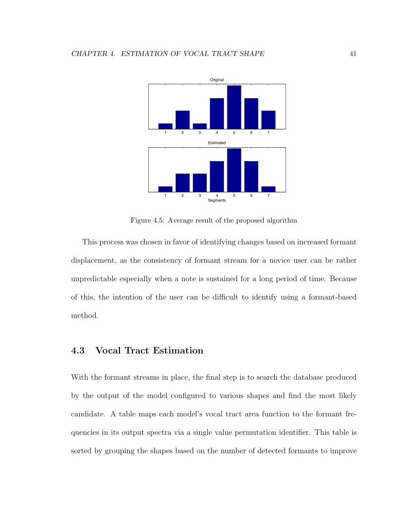
CHAPTER 4. ESTIMATION OF VOCAL TRACT SHAPE 41
1 2 3 4 5 6 7
Original
1 2 3 4 5 6 7Segments
Estimated
Figure 4.5: Average result of the proposed algorithm
This process was chosen in favor of identifying changes based on increased formant
displacement, as the consistency of formant stream for a novice user can be rather
unpredictable especially when a note is sustained for a long period of time. Because
of this, the intention of the user can be difficult to identify using a formant-based
method.
4.3 Vocal Tract Estimation
With the formant streams in place, the final step is to search the database produced
by the output of the model configured to various shapes and find the most likely
candidate. A table maps each model’s vocal tract area function to the formant fre-
quencies in its output spectra via a single value permutation identifier. This table is
sorted by grouping the shapes based on the number of detected formants to improve
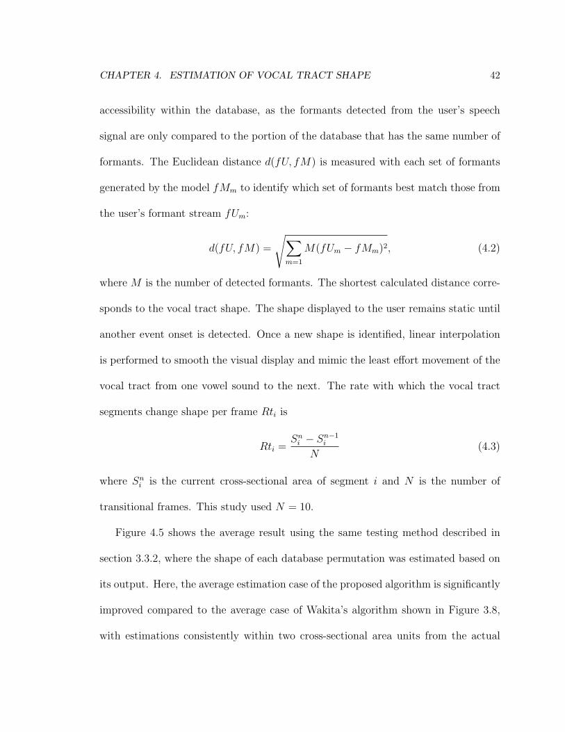
CHAPTER 4. ESTIMATION OF VOCAL TRACT SHAPE 42
accessibility within the database, as the formants detected from the user’s speech
signal are only compared to the portion of the database that has the same number of
formants. The Euclidean distance d(fU, fM) is measured with each set of formants
generated by the model fMm to identify which set of formants best match those from
the user’s formant stream fUm:
d(fU, fM) =
��
m=1
M(fUm − fMm)2, (4.2)
where M is the number of detected formants. The shortest calculated distance corre-
sponds to the vocal tract shape. The shape displayed to the user remains static until
another event onset is detected. Once a new shape is identified, linear interpolation
is performed to smooth the visual display and mimic the least effort movement of the
vocal tract from one vowel sound to the next. The rate with which the vocal tract
segments change shape per frame Rti is
Rti =Sn
i − Sn−1i
N(4.3)
where Sni is the current cross-sectional area of segment i and N is the number of
transitional frames. This study used N = 10.
Figure 4.5 shows the average result using the same testing method described in
section 3.3.2, where the shape of each database permutation was estimated based on
its output. Here, the average estimation case of the proposed algorithm is significantly
improved compared to the average case of Wakita’s algorithm shown in Figure 3.8,
with estimations consistently within two cross-sectional area units from the actual
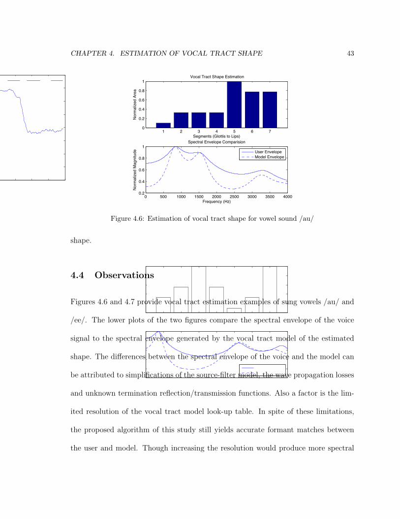
CHAPTER 4. ESTIMATION OF VOCAL TRACT SHAPE 43
0 0.5 1 1.5 2 2.5 3 3.5 40
0.1
0.2
0.3
0.4
0.5
0.6
0.7
0.8
Time (seconds)
Ampl
itude
ee oo ee
Figure 6. Amplitude envelope produced when voicing vow-els /ee/ then /oo/ then back to /ee/ while attempting to keepthe amplitude (loudness) constant. The amplitude envelopeclearly shows the locations of these event changes.
didate.A piecewise cylindrical waveguide model, similar to that
shown in Figure 1, was developed having Ns sections, eachwith NA possible cross-sectional area values, yieldingNNs
Apossible combinations. Considering all possible combina-tions yields duplicate shapes however, fewer correspondingvocal tract area functions are produced by considering onlythe change in cross section. Here, Ns = 7 and NA = 5seemed to produce the best results when considering perfor-mance, usability and accuracy, and the intended applicationof real-time musical control.A table maps the model’s vocal tract area function to the
formant frequencies in its output spectra. The table is sortedby grouping the shapes based on the number of detected for-mants. The formants detected from the incoming speechsignal (as described in Section 3) are compared to the en-tire portion of the database having the same number of for-mants. The Euclidean distance d(fU, fM) is used to mea-sure which set of formants generated by the model fMm
best match those generated by the user fUm:
d(fU, fM) =
����M�
m=1
(fUm − fMm)2, (9)
whereM is the number of detected formants. The estimatedvocal tract shape displayed to the user remains static untilanother event onset is detected. Once a new shape is identi-fied, linear interpolation is performed over the next frame tosmooth the transition, and thus the visual display, betweenthe two shapes.
6 RESULTS AND CONCLUSIONS
Figures 7 and 8 provide vocal tract estimation examples ofsung vowels /au/ and /ee/. The lower plots of the two fig-
1 2 3 4 5 6 70
0.2
0.4
0.6
0.8
1
Segments (Glottis to Lips)N
orm
aliz
ed A
rea
Vocal Tract Shape Estimation
0 500 1000 1500 2000 2500 3000 3500 40000.2
0.4
0.6
0.8
1
Frequency (Hz)
Nor
mal
ized
Mag
nitu
deSpectral Envelope Comparision
User EnvelopeModel Envelope
Figure 7. Estimation of vocal tract shape for vowel sound/au/.
1 2 3 4 5 6 70
0.2
0.4
0.6
0.8
1
Segments (Glottis to Lips)
Nor
mal
ized
Are
a
Vocal Tract Shape Estimation
0 500 1000 1500 2000 2500 3000 3500 40000
0.2
0.4
0.6
0.8
1
Frequency (Hz)
Nor
mal
ized
Mag
nitu
de
Spectral Envelope Comparision
User EnvelopeModel Envelope
Figure 8. Estimation of vocal tract shape for vowel sound/ee/.
Figure 9. Pure Data object displaying /au/ example
Figure 4.6: Estimation of vocal tract shape for vowel sound /au/
shape.
4.4 Observations
Figures 4.6 and 4.7 provide vocal tract estimation examples of sung vowels /au/ and
/ee/. The lower plots of the two figures compare the spectral envelope of the voice
signal to the spectral envelope generated by the vocal tract model of the estimated
shape. The differences between the spectral envelope of the voice and the model can
be attributed to simplifications of the source-filter model, the wave propagation losses
and unknown termination reflection/transmission functions. Also a factor is the lim-
ited resolution of the vocal tract model look-up table. In spite of these limitations,
the proposed algorithm of this study still yields accurate formant matches between
the user and model. Though increasing the resolution would produce more spectral
CHAPTER 4. ESTIMATION OF VOCAL TRACT SHAPE 44
0 0.5 1 1.5 2 2.5 3 3.5 40
0.1
0.2
0.3
0.4
0.5
0.6
0.7
0.8
Time (seconds)
Ampl
itude
ee oo ee
Figure 6. Amplitude envelope produced when voicing vow-els /ee/ then /oo/ then back to /ee/ while attempting to keepthe amplitude (loudness) constant. The amplitude envelopeclearly shows the locations of these event changes.
didate.A piecewise cylindrical waveguide model, similar to that
shown in Figure 1, was developed having Ns sections, eachwith NA possible cross-sectional area values, yieldingNNs
Apossible combinations. Considering all possible combina-tions yields duplicate shapes however, fewer correspondingvocal tract area functions are produced by considering onlythe change in cross section. Here, Ns = 7 and NA = 5seemed to produce the best results when considering perfor-mance, usability and accuracy, and the intended applicationof real-time musical control.A table maps the model’s vocal tract area function to the
formant frequencies in its output spectra. The table is sortedby grouping the shapes based on the number of detected for-mants. The formants detected from the incoming speechsignal (as described in Section 3) are compared to the en-tire portion of the database having the same number of for-mants. The Euclidean distance d(fU, fM) is used to mea-sure which set of formants generated by the model fMm
best match those generated by the user fUm:
d(fU, fM) =
����M�
m=1
(fUm − fMm)2, (9)
whereM is the number of detected formants. The estimatedvocal tract shape displayed to the user remains static untilanother event onset is detected. Once a new shape is identi-fied, linear interpolation is performed over the next frame tosmooth the transition, and thus the visual display, betweenthe two shapes.
6 RESULTS AND CONCLUSIONS
Figures 7 and 8 provide vocal tract estimation examples ofsung vowels /au/ and /ee/. The lower plots of the two fig-
1 2 3 4 5 6 70
0.2
0.4
0.6
0.8
1
Segments (Glottis to Lips)
Nor
mal
ized
Are
a
Vocal Tract Shape Estimation
0 500 1000 1500 2000 2500 3000 3500 40000.2
0.4
0.6
0.8
1
Frequency (Hz)
Nor
mal
ized
Mag
nitu
de
Spectral Envelope Comparision
User EnvelopeModel Envelope
Figure 7. Estimation of vocal tract shape for vowel sound/au/.
1 2 3 4 5 6 70
0.2
0.4
0.6
0.8
1
Segments (Glottis to Lips)N
orm
aliz
ed A
rea
Vocal Tract Shape Estimation
0 500 1000 1500 2000 2500 3000 3500 40000
0.2
0.4
0.6
0.8
1
Frequency (Hz)
Nor
mal
ized
Mag
nitu
de
Spectral Envelope Comparision
User EnvelopeModel Envelope
Figure 8. Estimation of vocal tract shape for vowel sound/ee/.
Figure 9. Pure Data object displaying /au/ example
Figure 4.7: Estimation of vocal tract shape for vowel sound /ee/
envelopes for comparison, it would increase the number of permutations and pos-
sibly adversely affect real-time performance without necessarily improving estimate
accuracy.
Chapter 5
Conclusions and Future Work
In this study, a real-time vocal tract area function estimation method is proposed that
matches the user’s formants to those produced by a piecewise cylindrical waveguide
model having an assumed similar shape. Estimations are made due to the relationship
between the vocal tract shape and formant placement within the magnitude spectrum.
The positioning of the user’s formants provide a way to match the formants of the
user to a particular vocal tract model shape, as the digital waveguide model simulates
the vocal tract’s effect on the propagating glottal source.
Formants are identified by detecting local maxima from the spectral envelope.
Formants detected from the frequency response of each waveguide model shape are
compiled offline within a sorted database that groups the shapes based their number
of formants. This process was done to reduce calculations and improve accessibility
within the database.
45
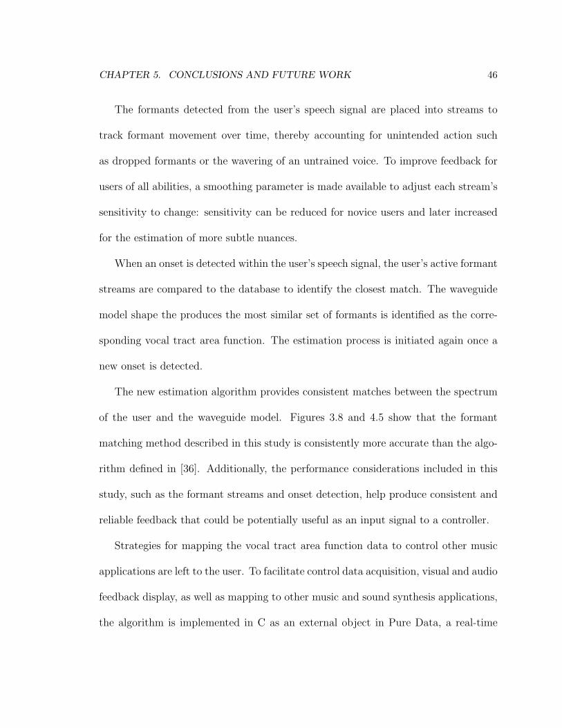
CHAPTER 5. CONCLUSIONS AND FUTURE WORK 46
The formants detected from the user’s speech signal are placed into streams to
track formant movement over time, thereby accounting for unintended action such
as dropped formants or the wavering of an untrained voice. To improve feedback for
users of all abilities, a smoothing parameter is made available to adjust each stream’s
sensitivity to change: sensitivity can be reduced for novice users and later increased
for the estimation of more subtle nuances.
When an onset is detected within the user’s speech signal, the user’s active formant
streams are compared to the database to identify the closest match. The waveguide
model shape the produces the most similar set of formants is identified as the corre-
sponding vocal tract area function. The estimation process is initiated again once a
new onset is detected.
The new estimation algorithm provides consistent matches between the spectrum
of the user and the waveguide model. Figures 3.8 and 4.5 show that the formant
matching method described in this study is consistently more accurate than the algo-
rithm defined in [36]. Additionally, the performance considerations included in this
study, such as the formant streams and onset detection, help produce consistent and
reliable feedback that could be potentially useful as an input signal to a controller.
Strategies for mapping the vocal tract area function data to control other music
applications are left to the user. To facilitate control data acquisition, visual and audio
feedback display, as well as mapping to other music and sound synthesis applications,
the algorithm is implemented in C as an external object in Pure Data, a real-time
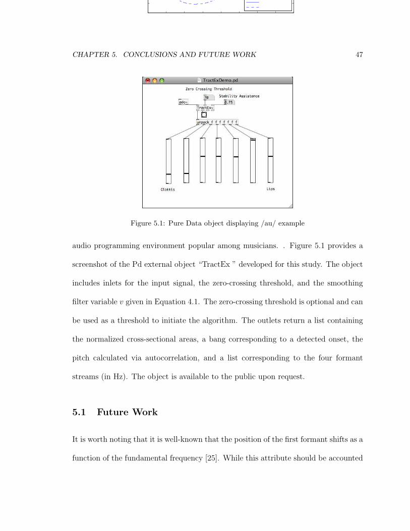
CHAPTER 5. CONCLUSIONS AND FUTURE WORK 47
0 0.5 1 1.5 2 2.5 3 3.5 40
0.1
0.2
0.3
0.4
0.5
0.6
0.7
0.8
Time (seconds)
Ampl
itude
ee oo ee
Figure 6. Amplitude envelope produced when voicing vow-els /ee/ then /oo/ then back to /ee/ while attempting to keepthe amplitude (loudness) constant. The amplitude envelopeclearly shows the locations of these event changes.
didate.A piecewise cylindrical waveguide model, similar to that
shown in Figure 1, was developed having Ns sections, eachwith NA possible cross-sectional area values, yieldingNNs
Apossible combinations. Considering all possible combina-tions yields duplicate shapes however, fewer correspondingvocal tract area functions are produced by considering onlythe change in cross section. Here, Ns = 7 and NA = 5seemed to produce the best results when considering perfor-mance, usability and accuracy, and the intended applicationof real-time musical control.A table maps the model’s vocal tract area function to the
formant frequencies in its output spectra. The table is sortedby grouping the shapes based on the number of detected for-mants. The formants detected from the incoming speechsignal (as described in Section 3) are compared to the en-tire portion of the database having the same number of for-mants. The Euclidean distance d(fU, fM) is used to mea-sure which set of formants generated by the model fMm
best match those generated by the user fUm:
d(fU, fM) =
����M�
m=1
(fUm − fMm)2, (9)
whereM is the number of detected formants. The estimatedvocal tract shape displayed to the user remains static untilanother event onset is detected. Once a new shape is identi-fied, linear interpolation is performed over the next frame tosmooth the transition, and thus the visual display, betweenthe two shapes.
6 RESULTS AND CONCLUSIONS
Figures 7 and 8 provide vocal tract estimation examples ofsung vowels /au/ and /ee/. The lower plots of the two fig-
1 2 3 4 5 6 70
0.2
0.4
0.6
0.8
1
Segments (Glottis to Lips)
Nor
mal
ized
Are
a
Vocal Tract Shape Estimation
0 500 1000 1500 2000 2500 3000 3500 40000.2
0.4
0.6
0.8
1
Frequency (Hz)
Nor
mal
ized
Mag
nitu
de
Spectral Envelope Comparision
User EnvelopeModel Envelope
Figure 7. Estimation of vocal tract shape for vowel sound/au/.
1 2 3 4 5 6 70
0.2
0.4
0.6
0.8
1
Segments (Glottis to Lips)
Nor
mal
ized
Are
a
Vocal Tract Shape Estimation
0 500 1000 1500 2000 2500 3000 3500 40000
0.2
0.4
0.6
0.8
1
Frequency (Hz)
Nor
mal
ized
Mag
nitu
de
Spectral Envelope Comparision
User EnvelopeModel Envelope
Figure 8. Estimation of vocal tract shape for vowel sound/ee/.
Figure 9. Pure Data object displaying /au/ exampleFigure 5.1: Pure Data object displaying /au/ example
audio programming environment popular among musicians. . Figure 5.1 provides a
screenshot of the Pd external object “TractEx ” developed for this study. The object
includes inlets for the input signal, the zero-crossing threshold, and the smoothing
filter variable v given in Equation 4.1. The zero-crossing threshold is optional and can
be used as a threshold to initiate the algorithm. The outlets return a list containing
the normalized cross-sectional areas, a bang corresponding to a detected onset, the
pitch calculated via autocorrelation, and a list corresponding to the four formant
streams (in Hz). The object is available to the public upon request.
5.1 Future Work
It is worth noting that it is well-known that the position of the first formant shifts as a
function of the fundamental frequency [25]. While this attribute should be accounted
CHAPTER 5. CONCLUSIONS AND FUTURE WORK 48
for in future work, the shift is fairly negligible due to the rather small bandwidth of
even the most significant displacement, whereas the upper formants appear unaffected
by a change in pitch. This study proposes that a more thorough examination must
be done to analyze how this shift varies from user to user in order to compensate
appropriately based on pitch. Preliminary observations have shown that this shift is
rather different between vocalists.
If more segments are deemed useful for the proposed vocal tract estimation algo-
rithm, search algorithms must be considered to ensure real-time performance. Strate-
gies such as simulated annealing, particle swarm, and multidimensional search trees
(kd-tree) have all been considered as potential solutions. Based on early results, the
formant database appeared prone to many local minima, thereby limiting the effec-
tiveness of each algorithm.
Bibliography
[1] Pd. http://www.pure-data.org.
[2] J. Bello, L. Daudet, S. Abdallah, C. Duxbury, M. Davies, and M. Sandler. A turorial ononset detection in musical signals. In IEEE Trans. Speech and Audio Proc., volume 13,pages 1035–1047, 2005.
[3] P. Broersen. Finite sample criteria for autoregressive order selection. In IEEE Trans.
Signal Processing, volume 48, pages 3550–3558, 2000.
[4] P.P.R. Christensen and W. Strong. A comparison of three methods of extracting reso-nance information from predictor-coefficient coded speech. In IEEE Trans. on Acoust.
Speech Signal Process., volume 24, pages 8–14, 1976.
[5] J. Dang and K. Honda. Estimation of vocal tract shapes from speech sounds withphysiological articulatory model. Journal of Phonetics, 30:511–532, 2002.
[6] P. de la Cuadra, A. Master, and C. Sapp. Efficient pitch detection techniques forinteractive music. In Proceedings of the 2001 International Computer Music Conference,2001.
[7] S. Dixon. Onset detection revisited. In 9th International Conference on Digital Audio
Effects, pages 133–137, 2006.
[8] S. Dubnov. Generalization of spectral flatness measure for non-gaussian linear pro-cesses. IEEE Signal Processing Letters, 11:698–701, 2004.
[9] J. L. Flanagan. Speech Analysis, Synthesis, and Perception. Springer-Verlag, 1972.
[10] V. Florian, G. McCaig, M. Ali, and S. Feis. Tongue n groove: an ultrasound basedmusic controller. In Proc. New Interfaces for Musical Expression, 2002.
[11] F. Gouyon, F. Pachet, and O. Delerue. On the use of zero-crossing rate for an appli-cation of classification of percussive sounds. In Proc. of the COST G-6 Conference on
Digital Audio Effects, 2000.
[12] T. Hankins and R. Silverman. Instruments and the Imagination. Princeton UniversityPress, 1999.
49
BIBLIOGRAPHY 50
[13] A. Hazan. Performing expressive rhythms with billaboop voice-driven drum generator.In Proc. of the 8th Int. Conference on Digital Audio Effects, 2002.
[14] Cater J. Electronically Speaking: Computer Speech Generation. Sams Publishing, 1983.
[15] J. Janer and M. de Boer. Extending voice-driven synthesis to audio mosaicing. In 5th
Sound and Music Computing Conference, 2008.
[16] J. A. Jenkin, F.and Ewing. Helmholt’s vowel theory and the phonograph. In Nature,pages 93–94, 1878.
[17] C. Jindai, J. Gangji, and Z. Lihe. A new method for extracting speech formants usinglpc phase spectrum. IEEE Electronics Letters, 29:2081–2082, 1993.
[18] A. Kestian and T. Smyth. Real-time estimation of the vocal tract shape for musicalcontrol. In Sound and Music Computing Conference, pages 206–211, 2008.
[19] P. Ladefoged, R. Harshman, L. Goldstein, and L. Rice. Generating vocal tract shapesfrom formant frequencies. J. Acoust. Soc. Am., 64:1027–1035, 1978.
[20] M. Lyons, M. Haehnel, and N. Tetsutani. Designing, playing, and performing with avision-based mouth in- terface. In Proc. New Interfaces for Musical Expression, 2003.
[21] S. Park, D. Kim, J. Lee, and T. Yoon. Integrated speech training systems for hearingimpaired. In IEEE Trans. on Rehabilitation Engineering, volume 2, pages 189–196,1994.
[22] D. Paul. Estimation of the vocal tract shape from the acoustic waveform. PhD thesis,Massachusetts Inst. Technol., 1976.
[23] G. Peeters. A large set of audio features for sound description (similarity and classifi-cation) in the cuidado project. Cuidado Project Rep. Ircam, 2004.
[24] L. Raphael, G. Borden, and K. Harris. Speech Science Primer: Physiology, Acoustics,
and Perception of Speech. Lippincott, Williams Wilkins, 2006.
[25] A. Robel and X. Rodet. Efficient spectral envelope estimation and its application topitch shifting and envelope preservation. In Proc. of the 8th Int. Conference on Digital
Audio Effects, pages 30–35, 2005.
[26] D. Rossiter, D. Howard, and M. Downes. A real-time lpc-based vocal tract area displayfor voice develop- ment. Journal of Voice, 8:314–319, 1994.
[27] R. Rothenberg. A new inverse-filtering technique for deriving the glottal air flow wave-form during voicing. In J. Acous. Soc. Amer., volume 53, pages 1632–1645, 1973.
[28] X. Serra. Music Sound Modeling with Sinusoids plus Noise. Music Signal Processing.Swets and Zeitlinger, 1997.
BIBLIOGRAPHY 51
[29] M. Shah and P. Pandley. Areagram display for investigating the estimation of vocaltract shape for a speech training aid. In Proc. Symposium on Frontiers of Re- search
on Speech and Music, pages 121–124, 2003.
[30] J. O. Smith. Digital waveguide modeling of musical instruments.ccrma.stanford.edu/ jos/waveguide/. Ablex Publishing Corporation: Norwood,NJ, 2003.
[31] J. O. Smith. Spectral Audio Signal Processing, August 2010 Draft.ccrma.stanford.edu/ jos/sasp/, accessed 9/2/2010. online book.
[32] T. Smyth and A. Fathi. Voice synthesis using the generalized pressure controlled-valve.In Proceedings of ICMC 2008, pages 57–60, 2008.
[33] J. Q. Stewart. An electrical analogue of the vocal organs. In Nature, volume 110, pages311–312, 1922.
[34] R. Valentine. http://biometrics.cse.msu.edu/speech-production.gif, accessed11/12/2010. online book.
[35] F. Villaciencio, A. Robel, and X. Rodet. Improving lpc spectral envelope extractionof voiced speech by true-envelope estimation. In IEEE International Conference on
Acoustics, Speech, and Signal Processing, volume 1, 2006.
[36] H. Wakita. Direct estimation of the vocal-tract shape by inverse filtering of acousticspeech waveforms. In IEEE Trans. Audio Electracout., volume AU-21, pages 417–427,1973.
[37] H. Wakita. Estimation of vocal-tract shapes from acoustical analysis of the speechwave: the state of the art. In IEEE Trans. Acoust. Speech Signal Process, volumeASSP-27, pages 281–285, 1979.