real-time optimization of chemical processes optimization of chemical processes" dominique...
TRANSCRIPT
Real-Time Optimizationof Chemical Processes"
Dominique Bonvin, Grégory François and Gene Bunin Laboratoire d’Automatique
EPFL, Lausanne
SFGP, Lyon 2013

2
Real-Time Optimization of a Continuous Plant
Planning & Scheduling!
Decision Levels!Disturbances!
Market Fluctuations, Demand, Price!
Catalyst Decay, Changing Raw Material Quality!
Fluctuations in Pressure, Flowrates, Compositions!
Long termweek/month!
Medium termday!
Short termsecond/minute!
Real-Time Optimization!
Control!
Production RatesRaw Material Allocation!
Optimal Operating Conditions - Set Points!
Manipulated Variables!Measurements!
Measurements!
Measurements!
Changing conditions! Real-time adaptation!
Large-scale complex processes!
3
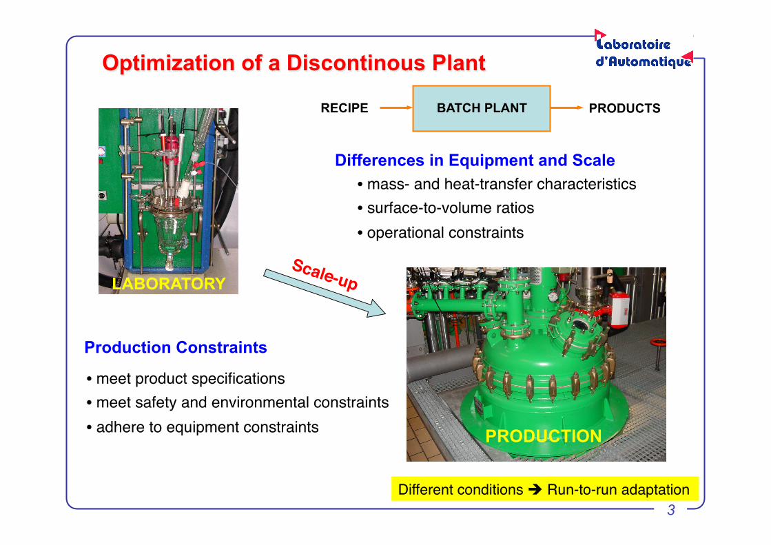
Optimization of a Discontinous Plant
Production Constraints
• meet product specifications!• meet safety and environmental constraints!• adhere to equipment constraints!
Differences in Equipment and Scale • mass- and heat-transfer characteristics!• surface-to-volume ratios!• operational constraints!
LABORATORY
Different conditions Run-to-run adaptation!
BATCH PLANT RECIPE PRODUCTS
Scale-up"
PRODUCTION
4
Outline
What is real-time optimization o Goal: Optimal plant operation o Tool: Model-based numerical optimization, experimental optimization o Key feature: use of real-time measurements
Real-time optimization framework
o Three approaches o Key issues: Which measurements? How to best exploit them? o Simulated comparison
Experimental case studies o Fuel-cell stack o Batch polymerization

5
Optimize the steady-state performance of a (dynamic) process !while satisfying a number of operating constraints!
Plant!
Static Optimization Problem
minu
Φ p u( ) := φp u, y p( )s. t. G p u( ) := g p u, y p( ) ≤ 0
(set points)!
? u"u
minu
Φ(u) := φ u, y( )
s. t. G u( ) := g u, y( ) ≤ 0 NLP"
Model-based Optimization!
?
F u, y,θ( ) = 0
(set points)!
? u"u
6
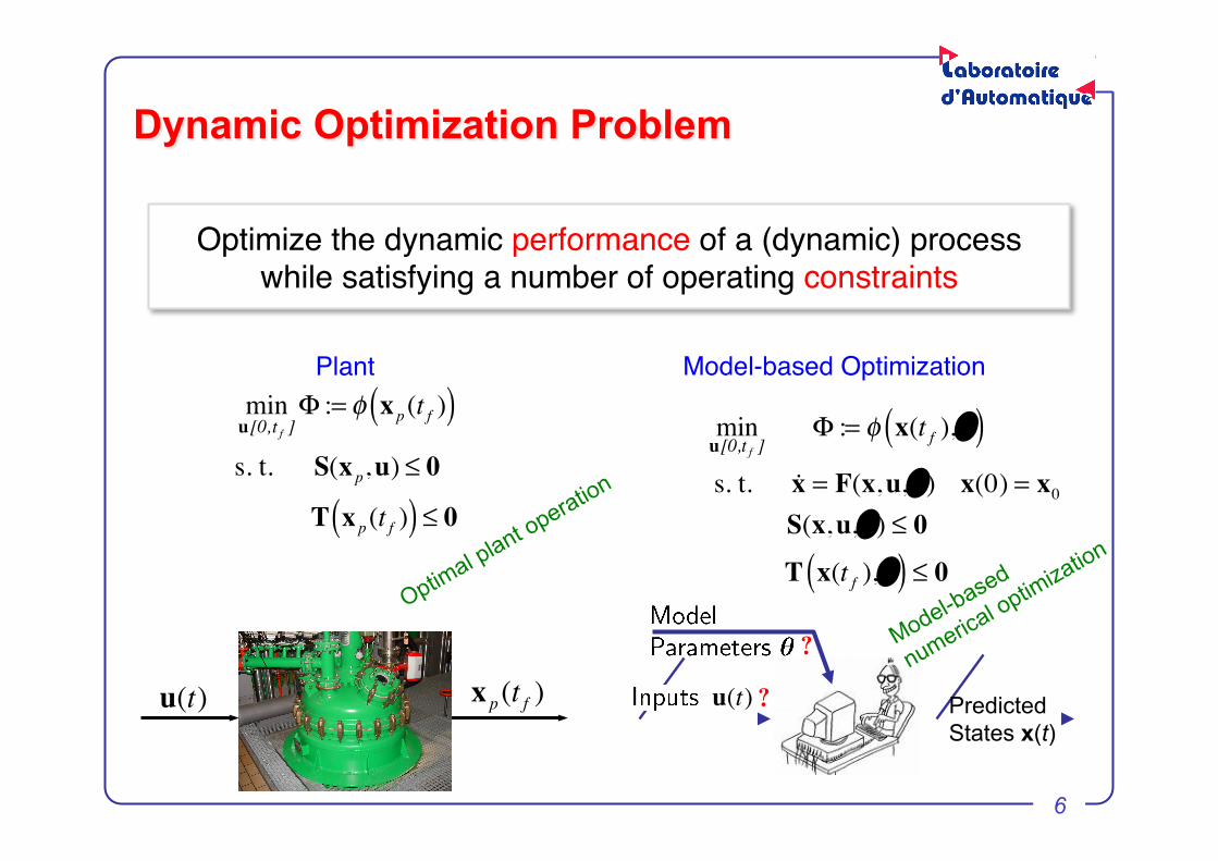
Optimize the dynamic performance of a (dynamic) process !while satisfying a number of operating constraints!
Plant!
Dynamic Optimization Problem
u(t) x p(t f )
minu[0,t f ]
Φ := φ x p(t f )( )s. t. S(x p,u) ≤ 0
T x p(t f )( ) ≤ 0
Model-based Optimization!
?
? u"u(t)
minu[0,t f ]
Φ := φ x(t f ),θ( )
s. t. x = F(x,u,θ ) x(0) = x0 S(x,u,θ ) ≤ 0
T x(t f ),θ( ) ≤ 0
Predicted States x(t)

7
Run-to-Run Optimization of a Batch Plant
minu[0,t f ]
Φ := φ x(t f ),θ( )
s. t. x = F(x,u,θ ) x(0) = x0 S(x,u,θ ) ≤ 0
T x(t f ),θ( ) ≤ 0
u(t) xp (t f )
Batch plant with!finite terminal time!
u[0,t f ] = U(π )Input Parameterization
u(t)!umax"
umin"tf"t1! t2!
u1!
0"
minπ
Φ π ,θ( )
s. t. G π ,θ( ) ≤ 0
Batch plant!viewed as a static map!
π Φ p
G p NLP"

8
Outline
What is real-time optimization o Goal: Optimal plant operation o Tool: Model-based numerical optimization, experimental optimization o Key feature: use of real-time measurements
Real-time optimization framework
o Three approaches o Key issues: Which measurements? How to best exploit them? o Simulated comparison
Experimental case studies o Fuel-cell stack o Batch polymerization

9
F
A, X
A,in= 1
F
B, X
B,in= 1
F = FA+ F
B
V
TR
XA, X
B, X
C, X
E, X
G, X
P
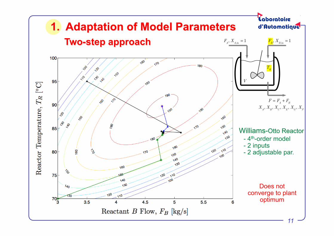
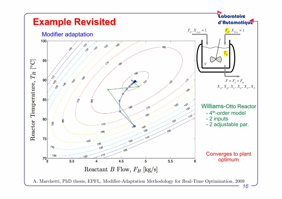
Example of Plant-Model Mismatch Williams-Otto reactor
3-reaction system A + B C B + C P + E C + P G
Objective: maximize operating profit
Model - 4th-order model - 2 inputs - 2 adjustable parameters (k10, k20)
2-reaction model A + 2B P + E A + B + P G
k2!
k1!
10
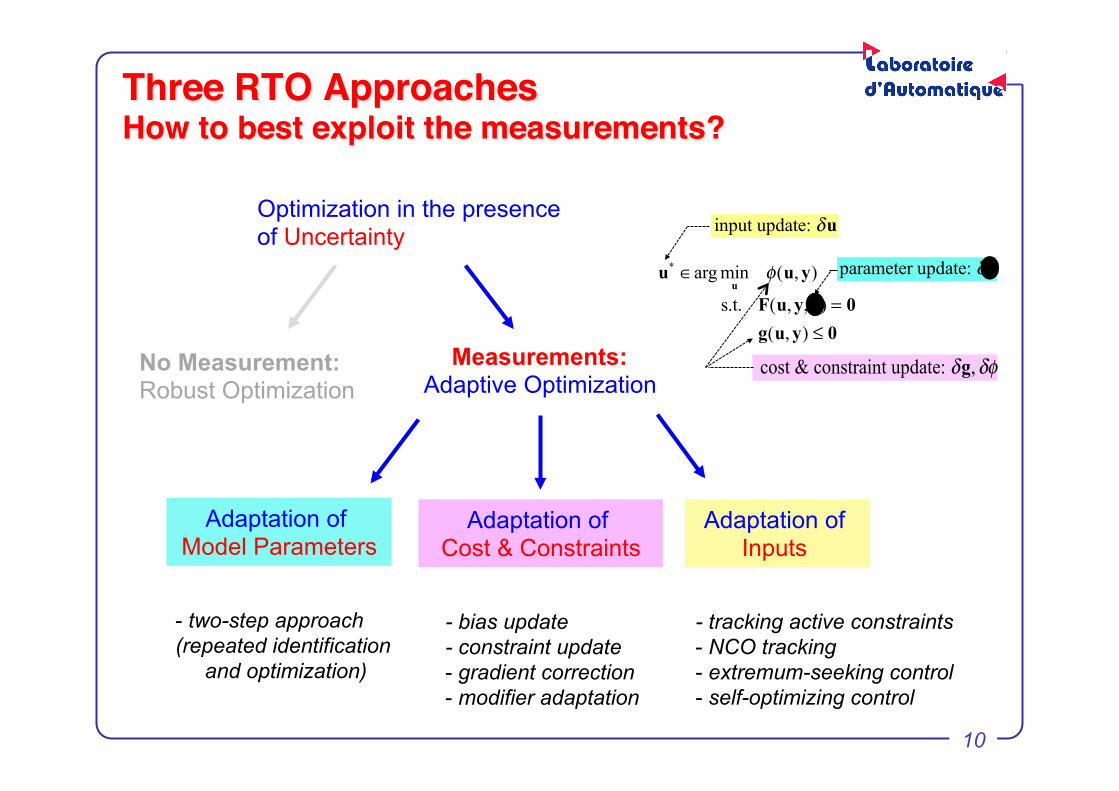
Three RTO ApproachesHow to best exploit the measurements?"
Optimization in the presence of Uncertainty
Measurements: Adaptive Optimization
No Measurement: Robust Optimization
u* ∈arg min
uφ(u, y)
s.t. F(u, y,θ) = 0g(u, y) ≤ 0
Adaptation of Inputs.
- tracking active constraints
- NCO tracking - extremum-seeking control - self-optimizing control
input update: δu
Adaptation of Model Parameters
- two-step approach (repeated identification and optimization)
parameter update: δθ
Adaptation of Cost & Constraints
- bias update
- constraint update
- gradient correction - modifier adaptation
cost & constraint update: δg,δφ
11
Does not converge to plant
optimum
Williams-Otto Reactor !- 4th-order model
- 2 inputs - 2 adjustable par.
F
A, X
A,in= 1
F
B, X
B,in= 1
F = FA+ F
B
V
TR
XA, X
B, X
C, X
E, X
G, X
P
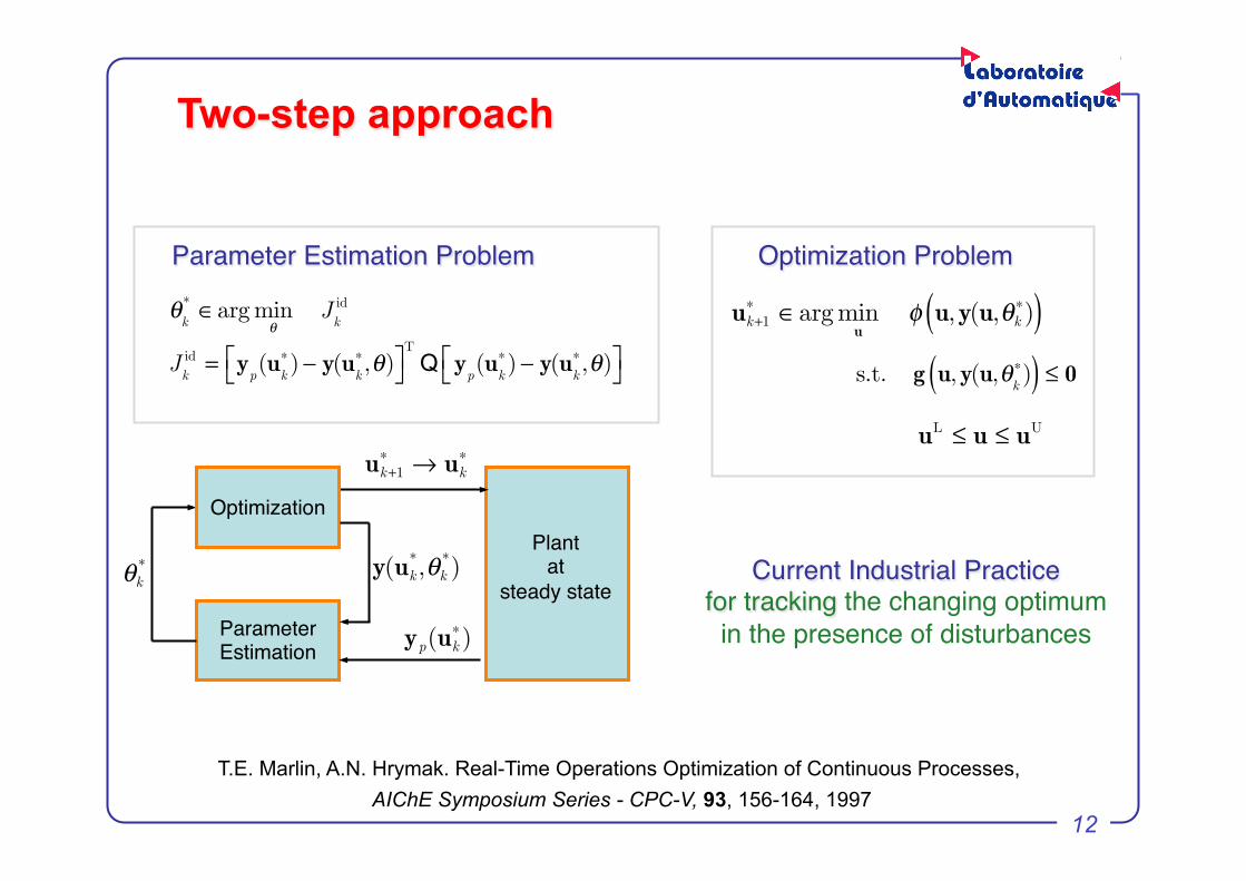
1. Adaptation of Model Parameters Two-step approach
12
Two-step approach
θ
k* ∈arg min
θJ
kid
J
kid = y
p(u
k∗)− y(u
k∗,θ)⎡⎣ ⎤⎦
TQ y
p(u
k∗)− y(u
k∗,θ)⎡⎣ ⎤⎦
s.t. g u,y(u,θ
k∗)( ) ≤ 0
Parameter Estimation Problem! Optimization Problem!
uk+1
∗ ∈argminu
φ u,y(u,θk∗)( )
uL ≤ u ≤ uU
Plant!at!
steady state!Parameter!Estimation!
Optimization!
uk+1∗ → uk
∗
θk*
yp(uk∗)
T.E. Marlin, A.N. Hrymak. Real-Time Operations Optimization of Continuous Processes, AIChE Symposium Series - CPC-V, 93, 156-164, 1997
Current Industrial Practice !for tracking the changing optimum!
in the presence of disturbances!
y(uk*,θk*)
13
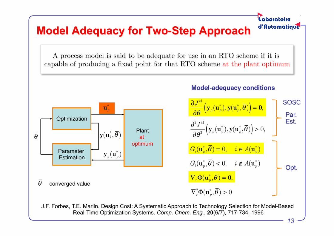
Model Adequacy for Two-Step Approach
J.F. Forbes, T.E. Marlin. Design Cost: A Systematic Approach to Technology Selection for Model-Based Real-Time Optimization Systems. Comp. Chem. Eng., 20(6/7), 717-734, 1996
A process model is said to be adequate for use in an RTO scheme if it is capable of producing a fixed point for that RTO scheme at the plant optimum
Model-adequacy conditions"
up∗
θ
yp(up∗ ) Gi(up
∗ ,θ ) = 0, i ∈A(up∗ )
Gi(up∗ ,θ ) < 0, i ∉A(up
∗ )
∇rΦ(up∗ ,θ ) = 0,
∇r2Φ(up
∗ ,θ ) > 0
Opt.!
∂J id
∂θyp(up
∗ ),y(up∗ ,θ )( ) = 0,
∂2J id
∂θ 2yp(up
∗ ),y(up∗ ,θ )( ) > 0,
Par.Est.!
SOSC!
converged value!θ
Plant!at !
optimum!Parameter Estimation!
Optimization!
y(uk*,θ )

14
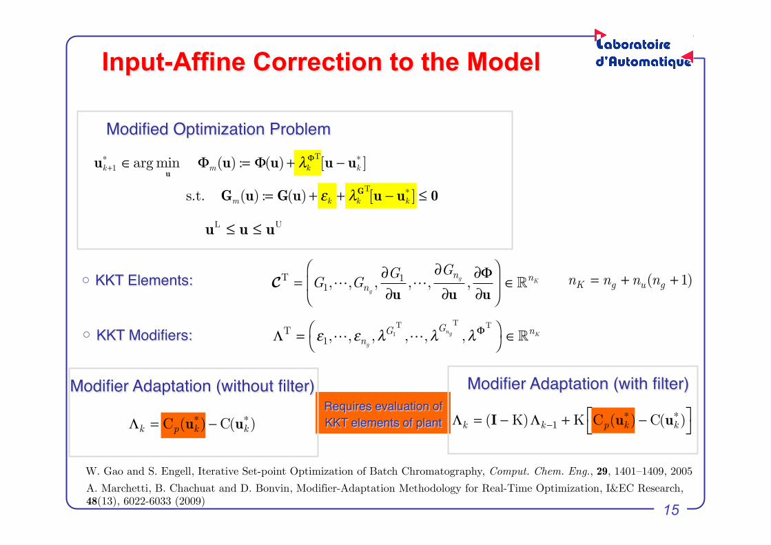
uk+1
∗ ∈arg minu
Φm(u) := Φ(u)+ λkΦ [u − uk
∗ ]
s.t. Gm(u) := G(u)+ εk + λkG [u − uk
∗ ] ≤ 0
Modified Optimization Problem!Affine corrections of cost and constraint functions!
uL ≤ u ≤ uU
T
T
2. Adaptation of Cost & Constraints Input-Affine Correction to the Model
Force the modified problem to satisfy the optimality conditions of the plant !
cons
train
t val
ue!
Gm(u)
Gp(u)
εk
G(u)
λkG [u − uk
∗ ]T
u uk
∗
P.D. Roberts and T.W. Williams, On an Algorithm for Combined System Optimization and Parameter Estimation, Automatica, 17(1), 199–209, 1981
15
Requires evaluation of KKT elements of plant!
uk+1
∗ ∈arg minu
Φm(u) := Φ(u)+ λkΦ [u − uk
∗ ]
s.t. Gm(u) := G(u)+ εk + λkG [u − uk
∗ ] ≤ 0
Modified Optimization Problem!
uL ≤ u ≤ uU
T
T
KKT Modifiers:!
KKT Elements:!
ΛT = ε1,,εng
,λG1 ,,λGng ,λΦ⎛⎝
⎞⎠ ∈nK
CT = G1,,Gng
,∂G1
∂u,,
∂Gng
∂u,∂Φ∂u
⎛
⎝⎜
⎞
⎠⎟ ∈nK
nK = ng + nu(ng + 1)
T T T
Λk = Cp(uk∗) −C(uk
∗)
Modifier Adaptation (without filter)!
Input-Affine Correction to the Model
Λk = (I − K)Λk−1 + K Cp(uk∗) −C(uk
∗)⎡⎣
⎤⎦
Modifier Adaptation (with filter)!
A. Marchetti, B. Chachuat and D. Bonvin, Modifier-Adaptation Methodology for Real-Time Optimization, I&EC Research, 48(13), 6022-6033 (2009)
W. Gao and S. Engell, Iterative Set-point Optimization of Batch Chromatography, Comput. Chem. Eng., 29, 1401–1409, 2005
16
Example Revisited F
A, X
A,in= 1
F
B, X
B,in= 1
F = FA+ F
B
V
TR
XA, X
B, X
C, X
E, X
G, X
P
Converges to plant optimum
Williams-Otto Reactor !- 4th-order model
- 2 inputs - 2 adjustable par.
Modifier adaptation
A. Marchetti, PhD thesis, EPFL, Modifier-Adaptation Methodology for Real-Time Optimization, 2009
17
Modeling for Optimization
Need to be able to estimate the plant gradients o From cost and constraint values at previous operating points o Must be able to use the key measurements (active constraints and
gradients)
Features of a “good” model
o Must be able to predict the optimality conditions of the plant: active constraints and (reduced) gradients
o Focuses on the optimal solution
“solution model” rather than “plant model”
18
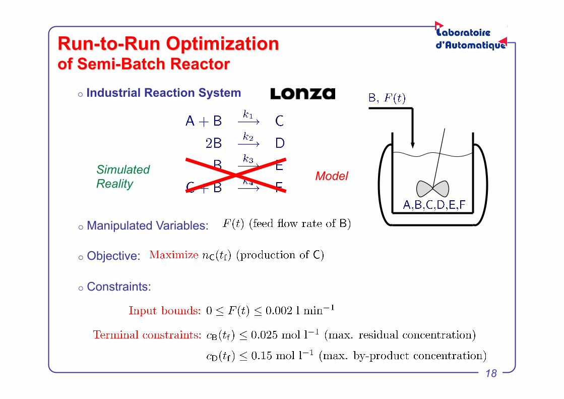
Run-to-Run Optimization of Semi-Batch Reactor
Objective:
Constraints:
Manipulated Variables:
Model
Industrial Reaction System
Simulated Reality
19
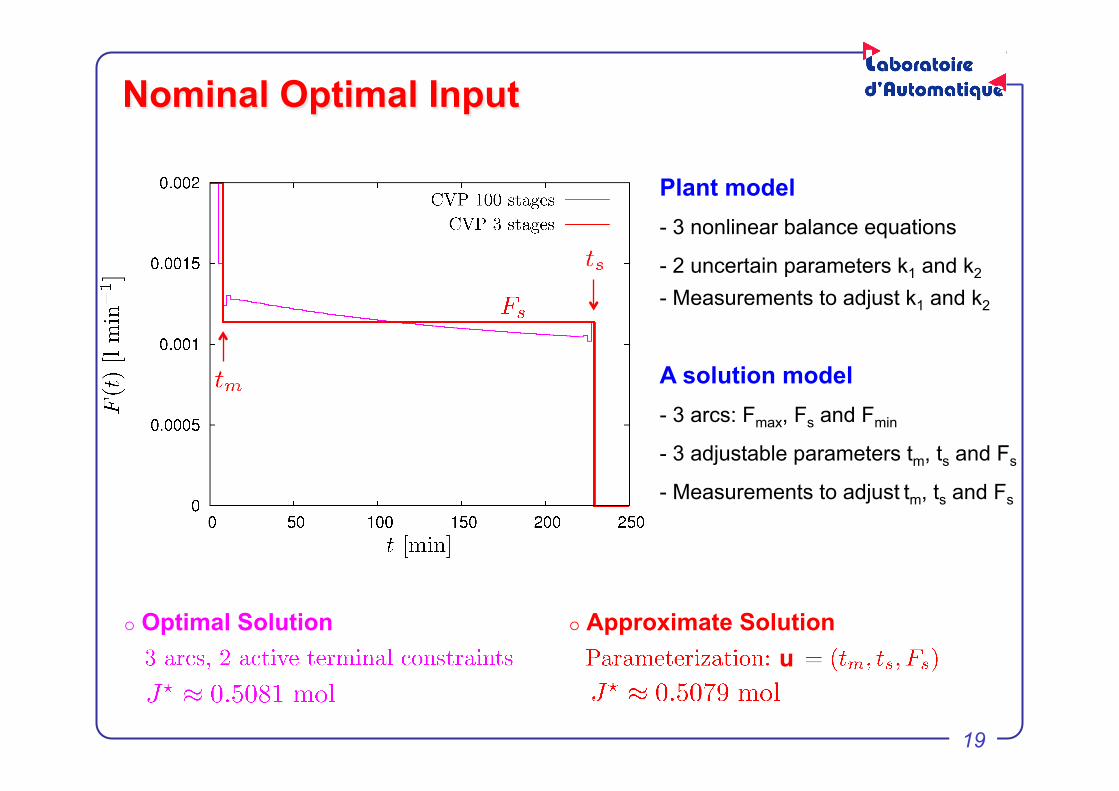
Nominal Optimal Input
Optimal Solution Approximate Solution u"
A solution model - 3 arcs: Fmax, Fs and Fmin
- 3 adjustable parameters tm, ts and Fs
- Measurements to adjust tm, ts and Fs
Plant model - 3 nonlinear balance equations
- 2 uncertain parameters k1 and k2
- Measurements to adjust k1 and k2

20
3. Adaptation of Inputs NCO tracking
Real Plant"Measurements!
Optimizing"Controller"
Feasibility OK!Optimal performance OK!
Disturbances!
Inputs ?!
Con
trol p
robl
em!Set points ?!
CV ?" MV ?"
NCO"cB(tf)=0.025!cD(tf)=0.15!
Available degrees of freedom"Input parameters"
ts, Fs!
Solu
tion
mod
el!
B. Srinivasan and D. Bonvin, Real-Time Optimization of Batch Processes by Tracking the Necessary Conditions of Optimality, I&EC Research, 46, 492-504 (2007).
21
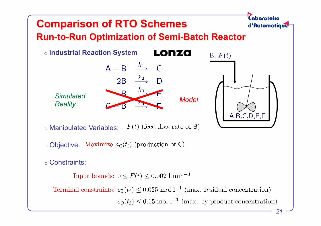
Comparison of RTO Schemes Run-to-Run Optimization of Semi-Batch Reactor
Objective:
Constraints:
Manipulated Variables:
Model
Industrial Reaction System
Simulated Reality

22
Adaptation of Model Parameters k1 and k2
Exponential Filter for k1, k2:
Identification Objective:
Measurement Noise: (10% constraint backoffs)
Large optimality loss!

23
Adaptation of Constraint Modifiers εG "
Exponential Filter for Modifiers:
No Gradient Correction
Measurement Noise: (10% constraint backoffs)
Recovers most of the optimality loss

24
Adaptation of Input Parameters ts and Fs
Controller Design:
No Gradient Correction
Measurement Noise: (10% constraint back-offs)
Recovers most of the optimality loss
tsk
Fsk
⎛
⎝⎜⎜
⎞
⎠⎟⎟=
tsk−1
Fsk−1
⎛
⎝⎜⎜
⎞
⎠⎟⎟
π = π k−1

25
Outline
What is real-time optimization o Goal: Optimal plant operation o Tool: Model-based numerical optimization, experimental optimization o Key feature: use of real-time measurements
Real-time optimization framework
o Three approaches o Key issues: Which measurements? How to best exploit them? o Simulated comparison
Experimental case studies o Fuel-cell stack o Batch polymerization
26
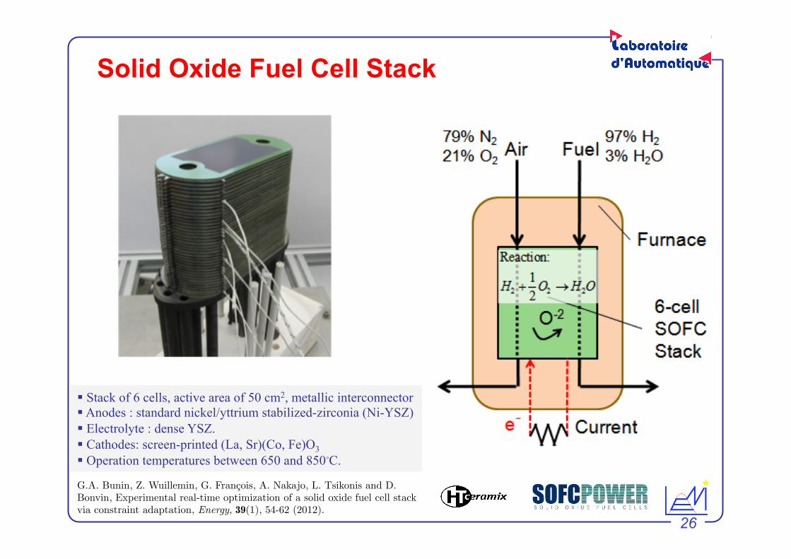
Stack of 6 cells, active area of 50 cm2, metallic interconnector Anodes : standard nickel/yttrium stabilized-zirconia (Ni-YSZ) Electrolyte : dense YSZ. Cathodes: screen-printed (La, Sr)(Co, Fe)O3 Operation temperatures between 650 and 850◦C.
G.A. Bunin, Z. Wuillemin, G. François, A. Nakajo, L. Tsikonis and D. Bonvin, Experimental real-time optimization of a solid oxide fuel cell stack via constraint adaptation, Energy, 39(1), 54-62 (2012).
Solid Oxide Fuel Cell Stack

27
RTO via Constraint Adaptation
Experimental features "
• Inputs: flowrates (H2, O2), current (or load)!
• Outputs: power density, cell potential, electrical efficiency!
• Time-scale separation!
slow temperature dynamics, treated as process drift ! !
static model (for the rest)!
• Power demand changes without prior knowledge!!• Inaccurate model in the operating region (power, cell)!
28
RTO via Constraint Adaptation
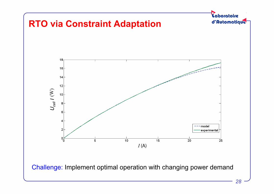
Challenge: Implement optimal operation with changing power demand
I (A)
p elAc
N cells(W)
Uce
ll I!
29
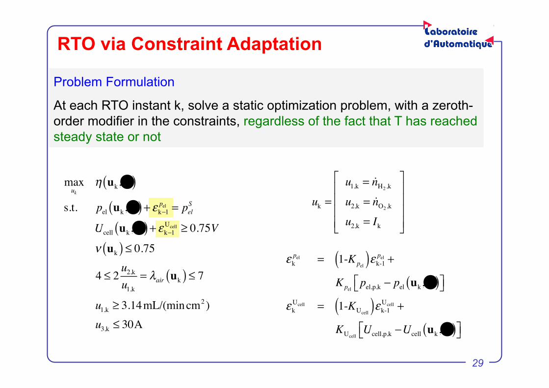
Problem Formulation At each RTO instant k, solve a static optimization problem, with a zeroth-order modifier in the constraints, regardless of the fact that T has reached steady state or not
maxuk
η uk,Θ( )s.t. pel uk,Θ( )+ εk−1pel = pelS
Ucell uk,Θ( )+ εk−1Ucell ≥ 0.75Vν uk( ) ≤ 0.75
4 ≤ 2u2,ku1,k
= λair uk( ) ≤ 7
u1,k ≥ 3.14mL/(mincm2)
u3,k ≤ 30A
uk =
u1,k = nH2,ku2,k = nO2,ku2,k = Ik
⎡
⎣
⎢⎢⎢⎢
⎤
⎦
⎥⎥⎥⎥
εkpel = 1-Kpel( )εk-1pel +
Kpelpel,p,k − pel uk,Θ( )⎡⎣ ⎤⎦
εkUcell = 1-KUcell( )εk-1Ucell +
KUcellUcell,p,k −Ucell uk,Θ( )⎡⎣ ⎤⎦
RTO via Constraint Adaptation

30
Slow RTO (“Wait for Steady State”)
!
RTO very 30 min! Unknown power changes every 90 min!
31
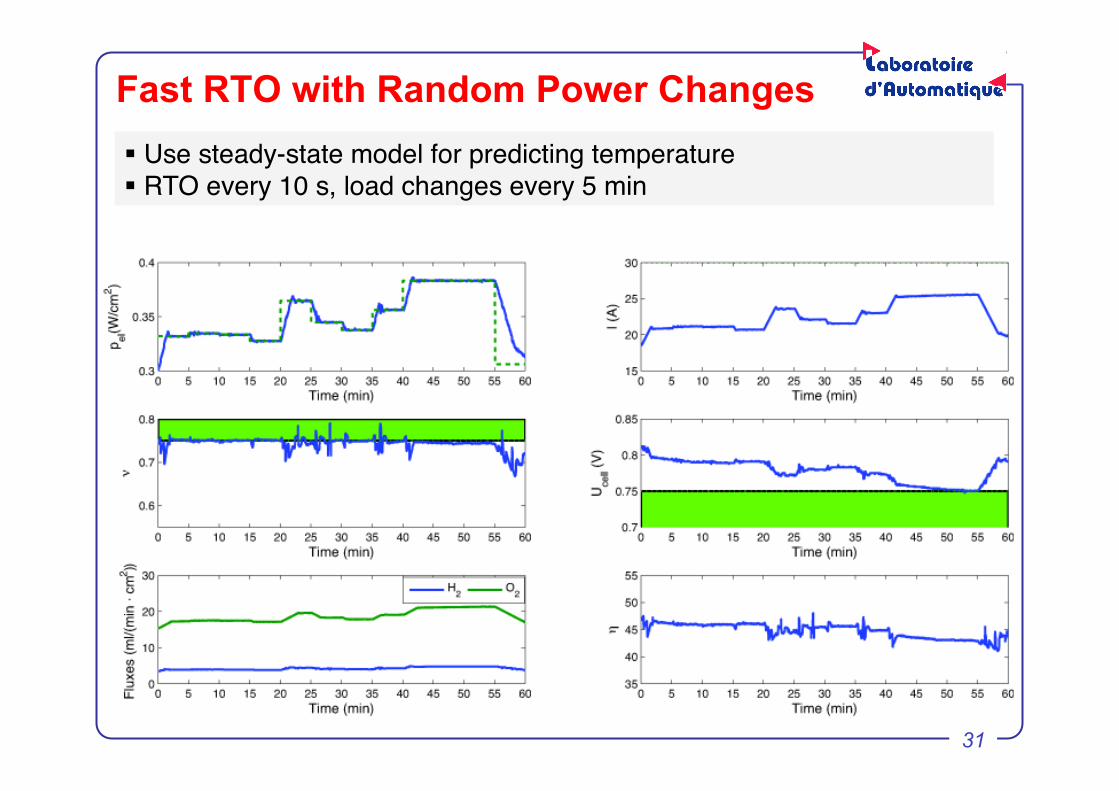
Fast RTO with Random Power Changes
Use steady-state model for predicting temperature ! RTO every 10 s, load changes every 5 min!
!

32
Industrial process!• 1-ton reactor, risk of runaway!
• Initiator efficiency can vary considerably!
• Several recipes!
different initial conditions!
different initiator feeding policies!
use of chain transfer agent!• Modeling difficulties!• Uncertainty!
�
Fj,T j,in
�
Tj
T (t)Mw (t)X(t)
⎫
⎬⎪
⎭⎪
Emulsion Copolymerization Process
Objective: Minimize batch time by adjusting the reactor temperature!• Temperature and heat removal constraints!
• Quality constraints at final time!
33
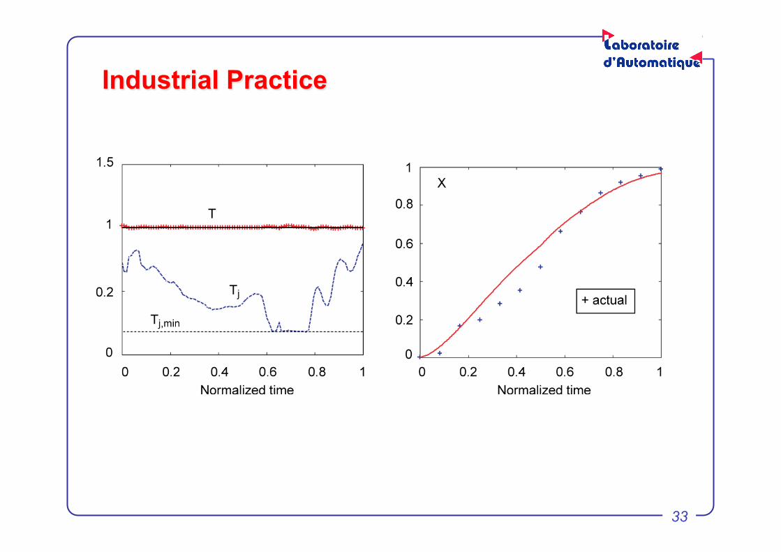
Industrial Practice

34
Optimal Temperature Profile Numerical Solution using a Tendency Model
• Current practice: isothermal!
• Numerical optimization! Piecewise-constant input! 5 decision variables (T2-T5, tf)! Fixed relative switching times!
0 0.2 0.4 0.6 0.8 10
0.5
1
1.5
2
time/tf [ ]
Piecewise Constant Optimal Temperature
Tr [ ]
Tr,max
Isothermal
Piecewise constant 2!1! 3! 4!
5!
Time tf
Tmax!
T [ ]!
• Active constraints! Interval 1: heat removal ! Interval 5: Tmax!
35
Model of the Solution Semi-adiabatic Profile!
ts!
t!
T(t)!
Tmax!
Tiso!
tf!
1!
2!Heat removal limitation ≈ isothermal operation
Compromise* ≈ adiabatic
T(tf) = Tmax!
ts enforces T(tf) = Tmax!
run-to-run adjustment of ts
*Compromise between conversion and quality

36
Final time!• Isothermal: 1.00 !• Batch 1: 0.78!• Batch 2: 0.72!• Batch 3: 0.65!
Batch 0"
1.0"
Industrial Results with NCO Tracking
Francois et al., Run-to-run Adaptation of a Semi-adiabatic Policy for the Optimization of an Industrial Batch Polymerization Process, I&EC Research, 43(23), 7238-7242, 2004
1-ton reactor

37
Conclusions
Two appoaches involving the NCO o Input-affine corrections to cost and constraints o NCO tracking (optimization via a multivariable control problem) o Key challenge is estimation of plant gradient
Process optimization is difficult in practice o Models are often inaccurate use real-time measurements o Repeated estimation and optimization lacks model adequacy o Which measurements? How to best exploit them? NCO (active constraints and reduced gradients)

38
NCO tracking New Paradigm for RTO
Operator-friendly approach o Start with best current operation (nominal model-based solution) and
push the process until constraints are reached o Know what to manipulate solution model o Determine how much to change from measurements
Important features o Two steps: offline (model-based), online (data-driven) o Can test robustness offline by using model perturbations o Approach converges to plant optimum, not model optimum o Complexity depends on the number of inputs (not system order) o Solution is partly determined by active constraints easy tracking o Price to pay: need to estimate experimental gradients