Real-Time Water Animation and Renderingusing Wavefront Parameter InterpolationMaster’s thesis in Complex Adaptive Systems

Gustav Olsson

Department of Computer Science and EngineeringChalmers University of TechnologyGothenburg, Sweden 2017

Master’s thesis 2017

Real-Time Water Animation and Rendering usingWavefront Parameter Interpolation

Gustav Olsson

Department of Computer Science and EngineeringComputer Graphics Research Group

Chalmers University of TechnologyGothenburg, Sweden 2017

Real-Time Water Animation and Rendering using Wavefront Parameter InterpolationGustav Olsson

c© Gustav Olsson, 2017.

Supervisor: Erik Sintorn, Department of Computer Science and EngineeringAdvisor: Fredrik Larsson and Jan Schmid, DICEExaminer: Ulf Assarsson, Department of Computer Science and Engineering

Master’s Thesis 2017Department of Computer Science and EngineeringComputer Graphics Research GroupChalmers University of TechnologySE-412 96 GothenburgTelephone +46 31 772 1000

Cover: Water waves refract around a natural jetty in a virtual depiction of theMediterranean coast implemented in the Frostbite [2017] game engine. The wateris simulated and rendered using the presented algorithm.

Typeset in LATEXGothenburg, Sweden 2017

iv

Real-Time Water Animation and Rendering using Wavefront Parameter Interpolation

Gustav Olsson

Department of Computer Science and Engineering

Chalmers University of Technology

Abstract

Realistic simulation and rendering of water is a challenge within the field of computergraphics because of its inherent multi-scale nature. When observing a large bodyof water such as the sea, there are small waves and perturbations visible close tothe observer. As the distance increases, the small scale details form large scale wavepatterns that may be several kilometers away.

A common approach to rendering large bodies of water in real-time is to simulatedeep water waves in a small area and repeat the wave motions across the watersurface at different spatial scales in order to minimize repetition patterns. Thismethod gives excellent results at open sea but cannot react to changes in waterdepth or the terrain of the virtual scene.

In this thesis, an algorithm for rendering large expanses of water that interact withthe terrain of the virtual scene in real-time is presented. The proposed algorithm firstsimulates water waves in a pre-computation step and saves wavefront parameterson a coarse triangle mesh as proposed by Jeschke and Wojtan [2015]. Then, thestored simulation is evaluated and the water surface is rendered in real-time using anovel staggered update scheme. The staggered update scheme effectively improvesthe rendering performance by a factor of 8 and makes it possible to render watersurfaces of up to 16 square kilometers with excellent visual quality and wave patternsat multiple spatial scales.

Keywords: computer graphics, water, ocean, wave, wavefront, terrain, wavefront parame-

ter interpolation, simulation, rendering, staggering

v

Contents

1 Introduction 11.1 Background . . . . . . . . . . . . . . . . . . . . . . . . . . . . . . . . 11.2 Purpose . . . . . . . . . . . . . . . . . . . . . . . . . . . . . . . . . . 21.3 Problem Statement . . . . . . . . . . . . . . . . . . . . . . . . . . . . 21.4 Limitations . . . . . . . . . . . . . . . . . . . . . . . . . . . . . . . . 2

2 Previous Work 3

3 Theory 63.1 Linear Wave Theory . . . . . . . . . . . . . . . . . . . . . . . . . . . 63.2 The Wavefront . . . . . . . . . . . . . . . . . . . . . . . . . . . . . . 9

4 Method 104.1 Overview . . . . . . . . . . . . . . . . . . . . . . . . . . . . . . . . . . 104.2 Simulation . . . . . . . . . . . . . . . . . . . . . . . . . . . . . . . . . 11

4.2.1 World Representation . . . . . . . . . . . . . . . . . . . . . . . 114.2.2 Coarse Mesh Generation . . . . . . . . . . . . . . . . . . . . . 114.2.3 Wavefront Generation . . . . . . . . . . . . . . . . . . . . . . 174.2.4 The Wavefront . . . . . . . . . . . . . . . . . . . . . . . . . . 184.2.5 The Simulation Step . . . . . . . . . . . . . . . . . . . . . . . 204.2.6 Wavefront Propagation . . . . . . . . . . . . . . . . . . . . . . 204.2.7 The Chain . . . . . . . . . . . . . . . . . . . . . . . . . . . . . 294.2.8 Wavefront Recording . . . . . . . . . . . . . . . . . . . . . . . 314.2.9 Combining Chains on Edges Into Wave Overlaps on Triangles 35

4.3 Rendering . . . . . . . . . . . . . . . . . . . . . . . . . . . . . . . . . 384.3.1 Water Surface Geometry . . . . . . . . . . . . . . . . . . . . . 384.3.2 Evaluating The Simulation . . . . . . . . . . . . . . . . . . . . 414.3.3 The Height-Lookup . . . . . . . . . . . . . . . . . . . . . . . . 45

5 Results 495.1 Performance . . . . . . . . . . . . . . . . . . . . . . . . . . . . . . . . 495.2 Achieved Visual Quality . . . . . . . . . . . . . . . . . . . . . . . . . 53

5.2.1 Overview . . . . . . . . . . . . . . . . . . . . . . . . . . . . . 535.2.2 Captured Water Wave Behaviors . . . . . . . . . . . . . . . . 56

6 Discussion 586.1 Cache Coherence . . . . . . . . . . . . . . . . . . . . . . . . . . . . . 59

7 Future Work 617.1 Coarse Mesh As Water Surface Geometry . . . . . . . . . . . . . . . . 617.2 Coarse Mesh Tree . . . . . . . . . . . . . . . . . . . . . . . . . . . . . 61

8 Conclusion 63

9 Acknowledgements 63

vii

1 Introduction

1.1 Background

As computers are increasingly being used to model the world, the importance ofcomputer graphics as a visualization tool increases. Rendering believable virtualscenes is important for any application that depicts the world in some way. Inaddition to being esthetically pleasing, a visualization provides intuition about thephenomenon under observation.

As water is abundant on Earth, there exists a need to render bodies of water invirtual scenes. For outdoor scenes, one would like to capture the grand scale of waterbehaviors present in everything from the open ocean and coastal areas to rivers andsmall lakes. In addition, one would like the transition between these areas to benatural and without seams.

Realistic simulation and rendering of water within the field of computer graphics isa difficult task. For real-time applications such as computer games or visualizationsoftware, a balance between realism and performance has to be made where theresult is convincing to an observer while at the same time allowing for interactiveframe rates (30-60 Hz). Graphical simulations of large expanses of water typicallyrestrict the simulation to 2 dimensions (a top-down view) and model deep waterwaves on the water surface using linear wave theory [Airy, 1841] (also known asAiry wave theory). In linear wave theory, a water wave is represented by its phase,amplitude, angular frequency and wavenumber and the water surface is assumed tobe a sum of waves evaluated as sinusoidal functions.

In order to render an ocean, one simplifies the model by assuming that all wavesare deep water waves that travel with constant speed independent of water depth.The Fast Fourier Transform is then used to generate and evolve a height map thatoffsets the geometry of the water surface to approximate the ocean [Tessendorf,2001]. To achieve real-time performance, several small height maps are typicallytiled across a large expanse of the ocean. The height maps are layered on topof each other at different spatial scales in order to minimize repetition patterns.This approach is excellent at capturing wind-driven deep water waves but is limitedwhen it comes to other types of waves. In particular, the major downside with thisapproach is that the water simulation can not interact naturally with coastlines orobjects that are submerged in the water, nor react to changes in water depth.

In reality, water waves refract when they move from one depth to another in thesame way light refracts as it moves from one medium to another. The reason waterwaves refract is that the speed of any point along a wave depends on the depth of thewater at that location. If the speed of points along the wave crest diverge, the waverefracts and the wave crest bends. Thus, the crest curves of water waves typicallybend towards areas of shallow waters since that is where the speed is low. In additionto refraction, water waves reflect when they collide with hard surfaces such as cliffsor stones that are submerged in the water. The reflecting waves superimpose on topof the ambient waves and cause ripples on the water surface that are sometimes asimportant to the appearance of coastal scenes as ambient wind-driven waves.

Thus, the natural next step towards increased realism is to take the terrain of thevirtual scene into account when simulating the water.

1

1.2 Purpose

The aim of this thesis is to develop an algorithm for simulating and rendering largeexpanses of water that interact with the terrain of the virtual scene. Furthermore,the algorithm must allow rendering of the water surface in real-time on currentgraphics hardware.

1.3 Problem Statement

The thesis will determine how to:

1. Robustly simulate waves that react to the terrain in a variety of differentvirtual scenes

2. Render the simulation in real-time on current graphics hardware while main-taining excellent visual quality

Robustly simulate waves that react to the terrain in a variety of different virtualscenes The proposed algorithm will be used in a production environment wherethere are high demands on the stability and predictability of the simulation. Thesimulation should not just produce accurate results for one or two example scenes, itmust perform reliably across a wide range of possible inputs crafted by artists withlittle knowledge of the inner workings of the algorithm.

Render the simulation in real-time on current graphics hardware while maintain-ing excellent visual quality Within the field of computer graphics, performanceand visual quality are tightly coupled and the proposed algorithm for rendering theocean needs to strike a balance between the two. The rendering of the simulationmust reach a frame rate of at least 60 Hz in order for the proposed algorithm tobe usable in practice. In addition, the visual quality of a rendered frame must beexcellent with no visible aliasing or noise.

1.4 Limitations

The scope of the thesis is limited to the animation of waves on the water surfaceand the basic rendering of the water surface geometry.

While there are numerous aspects that need to be considered when making virtualwater believable, the intention is not to write a thorough dissertation on all of them.In order to facilitate pre-computation of the simulation, the terrain of the virtualscene with which the waves interact is considered static and the effects of dynamicobjects submerged in the water are omitted. Non-linear effects of water waves suchas breaking waves and consequently foam and spray are not considered. Finally, theway light interacts with the volume of water and how it affects the shading of thewater surface is not considered.

2

2 Previous Work

Water surface rendering Bruneton et al. [2010] show how to accurately illumi-nate and render the ocean at all scales in real-time. Aliasing is eliminated usinga hierarchical representation that combines surface geometry, normals and BRDFin order to sample waves at the appropriate level of detail, respecting the Nyquistlimit.

There are several ways of constructing the geometry of the water surface. Kry-achko [2005] use a simple radial grid mesh centered around the camera and samplethe wave function at each vertex. The radial grid is densely sampled at the centerand becomes gradually more sparse as the distance from the camera increases. Jo-hanson and Lejdfors [2004] introduce the concept of a projected grid to achieve auniform resolution of vertices in screen space. A rectangular grid is constructed inscreen space and projected from the camera onto the water plane. Each projectedvertex is then used to sample the water surface, yielding samples of even spacing inscreen space and non-linear spacing in world space.

In order to offset the water surface, several authors turn to trochoid wave profiles[Tessendorf, 2001, Finch, 2004, Bruneton et al., 2010] originally discovered by Ger-stner [1809]. A trochoidal wave is an exact solution to the Euler fluid equations fordeep water gravity waves [Bruneton et al., 2010] where fluid parcels move in closedcircles.

Waves in homogenous media Tessendorf [2001] show how deep water waves canbe evolved in the Fourier domain in order to generate realistic height and normalmaps of the water surface. With the advent of programmable graphics hardware,their research has become the current state of the art for real-time water animationand rendering of large expanses of water.

Waves in heterogeneous media Waves propagating in heterogeneous media arestudied extensively in many areas of research and several simulation schemes forwave propagation have been developed. Rawlinson et al. [2008] provides a detailedreview of existing simulation schemes in the context of seismology. For a moregeneral overview, see Runborg [2007].

Fournier and Reeves [1986] and Peachey [1986] were the first to show how waverefraction close to shores can be achieved by varying the phase speed of waves. Theyuse the concept of a ”wave train” and a ”wave component”, respectively, to describea wave with a particular angular frequency, amplitude and propagation direction.The phase of each point along the wave is numerically integrated along a straightline path in the direction of propagation to produce a grid of phase values. The gridsare then used during rendering to evaluate the surface height of the water at anylocation in the world. These models capture wave refraction but are limited as thepropagation direction of a wave is held constant and only first-arrivals are accountedfor, i.e., only a single value of the multi-valued phase function is computed.

Ts’o and Barsky [1987] introduce the concept of ”wave-tracing” and let the prop-agation direction of a point on the wave change according to Snell’s law. The wave-tracing scheme is analogous to ray-tracing for arrival time computations within the

3

field of geometrical optics and seismology and conventional ray-tracing for light thatis used for image generation in Computer Graphics. For rendering, wave heights areevaluated and stored on a regular grid as rays pass close to the grid points. Thismethod allows for refraction and sharp changes in propagation direction in additionto multiple arrivals of a wave, i.e., many values of the multi-valued phase functionare captured. However, in areas where rays diverge, there will be insufficient raycoverage and the method will produce patches of undisturbed water on the surface.

Gonzato and Le Saec [1997] improve on the work of Ts’o and Barsky [1987] bytreating the wave as a wavefront and achieve a nearly constant spatial resolution ofrays across the water surface by subdividing and collapsing neighboring rays. Thispropagation scheme is known as wavefront construction in physical space withinthe wavefront tracking literature and was originally proposed by Vinje et al. [1993].Gonzato and Le Saec [2000] extend their method to capture wave reflection anddiffraction and render the water surface by ray-tracing the wavefronts stored atregular time intervals.

In order to reduce the memory requirements of previous methods, Jeschke andWojtan [2015] propose a two-dimensional unstructured coarse triangle mesh as ameans to store the recorded wave data. Reconstruction of the stored wave datais handled through a novel interpolation scheme that sidesteps the Nyquist limitand allows high-frequency waves to be captured even by a loosely tessellated coarsemesh. The coarse mesh is spatially adaptive and constructed by first generatinga point-set covering the water domain using Poisson disk sampling with the diskradius varying with the distance to the seabed boundary and then constructing theDelaunay triangulation of these points.

In order to interpolate wave data in wavefront construction schemes, inverse bi-linear interpolation must be used. Quilez [2010] describes a simple algorithm forcomputing the inverse bilinear interpolation of a set of four points.

Osher et al. [2002] introduce the concept of a bicharacteristic strip in reducedphase space in order to solve for the multi-valued phase function using a level setapproach within the field of geometric optics. A self-intersecting wavefront in worldspace becomes a non-self-intersecting curve in reduced phase space that is known asthe bicharacteristic strip. Hauser et al. [2006] compare an Eulerian and a Lagrangianapproach to solving the multi-valued phase function and show how the resolution ofLagrangian wavefronts can be maintained in reduced phase space.

Mesh generation Cook [1986] introduced Poisson disk sampling in the field ofComputer Graphics and showed how it can be used to reduce aliasing. Bridson[2007] developed a linear-time algorithm for Poisson disk sampling in arbitrary di-mensions. Poisson disk sampling can be extended to use variable radii and proofson the properties of the resulting point-set and subsequent Delaunay triangulationcan be made [Mitchell et al., 2012].

The Delaunay triangulation and its dual, the Voronoi diagram, have been studiedextensively within the field of Computational Geometry and Computer Graphicsand Aurenhammer [1991] provides a thorough dissertation on the subject. Incre-mental flipping is a common algorithm for constructing the Delaunay triangulationfrom a set of points that is proven to work in arbitrary dimensions [Edelsbrunner

4

and Shah, 1992]. Brown [1979] first showed that there is a relationship betweenn-dimensional Voronoi diagrams and n+1-dimensional convex hulls through a stere-ographic projection. Edelsbrunner and Seidel [1985] built upon Brown’s work andshowed that the Delaunay triangulation of an n-dimensional point-set is equivalentto an orthographic projection of the triangles of the convex hull of the points liftedto a n+1-dimensional parabola.

The convex hull is an important concept within the field of Computational Ge-ometry. In addition to being closely related to other important concepts such as theDelaunay triangulation and the Minkowski set, convex hulls can be used to simplifycomplex problems. Gilbert et al. [1988] showed that convex hulls and the Minkowskiset can be used for fast intersection and distance calculations between complex ob-jects. There are numerous algorithms for computing the convex hull of a point-set.Barber et al. [1996] developed an iterative algorithm that works in arbitrary di-mensions and has seen widespread adoption but is susceptible to precision errorswhen the input is not in general position. Gustafsson [2013] proposes a promis-ing topology-based algorithm that is robust against inputs not in general position.This algorithm for generating three-dimensional convex hulls seems to be related toincremental flipping for constructing the two-dimensional Delaunay triangulation.

See Ericson [2004] for a comprehensive summary of geometric concepts in the fieldof Computer Graphics.

Ocean wave spectra In oceanic research, one is interested in the shape of the seasurface in different weather conditions and several ocean wave spectra have beendeveloped to describe the state of the ocean given different parameters such as windspeed or fetch. Pierson and Moskowitz [1964] experimentally find a spectrum forfully developed seas which gives the energy density of the sea as a function of angularfrequency and wind speed.

5

3 Theory

The next section will introduce the theory necessary to follow the reasoning insubsequent sections.

3.1 Linear Wave Theory

Linear wave theory is a linear model for surface waves on a body of water. It wasfirst formulated by George Bidell Airy in the 19th century [Airy, 1841] and is alsocommonly known as Airy wave theory.

The model states that the water surface can be approximated by a sum of sinu-soidal functions:

η(~x, t) = η0 +N∑i=1

ai sin(ωiφi(~x)− ωit) (1)

where η(~x, t) is the water height at point ~x at time t, n0 a constant offset, N thenumber of waves and ai, ωi, φi the amplitude, angular frequency and phase functionof the i :th wave [Jeschke and Wojtan, 2015].

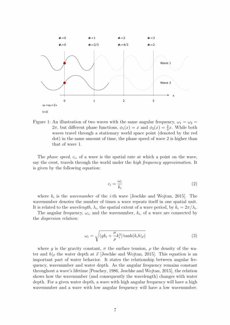
An important realisation is that two waves with the same angular frequency,oscillating at the same rate, can be different due to the phase function. Considera stationary world space point. Two waves, with the same angular frequency, passthrough the point (the point travels the length of an entire wave period) in thesame amount of time but the lateral speed at which they pass may be different. Ifwave A travels much faster than wave B, wave A will seem stretched out in relation.On the other hand, if wave A travels much slower than wave B, wave A will seemcompressed. Thus, for a wave, one can say that the angular frequency denotes thetemporal rate of the oscillations and the phase function denotes the spatial rate ofrepetition. See Figure 1 for an illustration of this concept.

6

x

ω₁=ω₂=2

t=0

3210

Wave 2

Wave 1

₁=2

₂=4/3

₁=3

₂=2

₁=1

₂=2/3

₁=0

₂=0

Figure 1: An illustration of two waves with the same angular frequency, ω1 = ω2 =2π, but different phase functions, φ1(x) = x and φ2(x) = 2

3x. While both

waves travel through a stationary world space point (denoted by the reddot) in the same amount of time, the phase speed of wave 2 is higher thanthat of wave 1.

The phase speed, ci, of a wave is the spatial rate at which a point on the wave,say the crest, travels through the world under the high frequency approximation. Itis given by the following equation:

ci =ωi

ki(2)

where ki is the wavenumber of the i :th wave [Jeschke and Wojtan, 2015]. Thewavenumber denotes the number of times a wave repeats itself in one spatial unit.It is related to the wavelength, λi, the spatial extent of a wave period, by ki = 2π/λi.

The angular frequency, ωi, and the wavenumber, ki, of a wave are connected bythe dispersion relation:

ωi =

√(gki +

σ

ρk3i ) tanh(kih|~x) (3)

where g is the gravity constant, σ the surface tension, ρ the density of the wa-ter and h|~x the water depth at ~x [Jeschke and Wojtan, 2015]. This equation is animportant part of water behavior. It states the relationship between angular fre-quency, wavenumber and water depth. As the angular frequency remains constantthroughout a wave’s lifetime [Peachey, 1986, Jeschke and Wojtan, 2015], the relationshows how the wavenumber (and consequently the wavelength) changes with waterdepth. For a given water depth, a wave with high angular frequency will have a highwavenumber and a wave with low angular frequency will have a low wavenumber.

7

This is intuitive as in real-life, waves with short wavelengths tend to oscillate quicklywhereas waves with long wavelengths tend to oscillate slowly.

Using the dispersion relation, one may express the phase speed ci as a function ofωi, ki and h|~x:

ci =ωi

ki=

√(g

ki+σ

ρki) tanh(kih|~x) (4)

In this form, it can be seen that the phase speed, i.e., the speed at which a wavepropagates, tends to infinity both as ki → 0 and ki → ∞, and increases with thedepth of the water. In addition, the phase speed is almost independent of waterdepth for capillary waves (large ki) and deep water waves (large h|~x) as tanh ≈ 1.

Under the high frequency approximation, a wave propagates according to theEikonal equation,

|∇φ| = 1

c, (5)

and travels through space with phase speed c [Jeschke and Wojtan, 2015]. Thedifference in phase between two world space points is then the time it takes for thewave to travel between the points. The high frequency approximation is formallyvalid in the limit when the angular frequency of a wave tends to infinity [Runborg,2007] and it is a good approximation when the wavelength is small compared tofeatures of the boundary domain. In particular, under the high frequency approxi-mation, a point on a wave travels in a straight line in homogeneous media and wavesdo not diffract when grazing obstacles. Rawlinson et al. [2008] show the derivationof the Eikonal equation from the elastic wave equation.

When water depth is constant, the phase speed is constant and thus the phase ofa wave is a linear function of distance, φi(x) = x/ci = kix/ωi, and the water surfaceis a sum of plane waves:

η(~x, t) = η0 +N∑i=1

ai sin(~ki · ~x− ωit)

where the wave vector ~ki denotes the direction of propagation with∣∣∣~ki∣∣∣ = ki.

However, when the water depth and consequently the phase speed is not constant,the phase function is non-linear and often multi-valued [Jeschke and Wojtan, 2015].

The energy density Di of wave i is given by:

Di =(ρg + σk2

i )a2i

2. (6)

Finally, energy propagates at the rate of the group speed :

cg =dω

dk. (7)

8

3.2 The Wavefront

It is straightforward to describe the motion of water waves using linear wave theoryfor water of uniform depth, as the waves travel at constant phase speed and can bedescribed by plane waves. However, when the seafloor is heterogeneous in depth,the wavenumber and consequently the phase speed of a wave will vary according tothe dispersion relation.

When viewing a water wave travelling in a heterogeneous depth field from above,different points on the wave will travel at different speeds and it is convenient tointroduce the concept of a wavefront. A wavefront is the set of points of constantphase away from a source. The points form a curve in R2.

As different points along a wavefront travel at different speeds, the wavefrontbends towards areas of lower speeds. This is what makes ocean waves that travelchaotically at sea line up with the coastline as they approach shallow waters.

An initially straight wavefront may bend, stretch and even fold over itself asit travels across the water surface. In practice, a wavefront will develop self-intersections even in a simple underlying depth field. An example of this is theswallowtail pattern that appears when a straight wavefront enters a circular area ofgradually slower speeds and bends over itself [Hauser et al., 2006]. See Figure 2 foran illustration of this phenomenon.

Figure 2: A wavefront forms a swallowtail pattern as it passes over a local low speedarea. Multiple time steps of the wavefront are shown transitioning fromgreen to red with increasing phase.

The observation that a wavefront can pass over a world space point multiple timesin a heterogeneous depth field provides intuition behind the multi-valued nature ofthe phase function. Each value of the phase function at a world space point describesa time the wavefront moved passed the point.

9

4 Method

The algorithm for animating and rendering the water surface was developed usingresearch in the field of computer graphics and oceanography as reference. The thesiscovers the subset of the accomplished work that is relevant according to the problemstatement.

The thesis project was carried out at the video game development company DICE[2017] in Stockholm, Sweden, and the algorithm was integrated into their in-housegame engine, Frostbite [2017].

4.1 Overview

The proposed algorithm for generating and rendering the ocean consists of twosteps: the simulation step and the rendering step. The simulation step is basedon the novel approach to wavefront construction developed by Jeschke and Wojtan[2015] in which wavefronts are propagated across a virtual scene and wave parame-ters are recorded as they pass over the triangles of a coarse 2-dimensional trianglemesh (coarse mesh) covering the ocean surface. The rendering step generates thegeometrical displacement and normals necessary to accurately render the ocean sur-face by sampling the recorded wave parameters stored on the coarse mesh. In orderto render the ocean at any spatial scale and provide a seamless transition betweendifferent levels of detail, individual waves are filtered by wavelength as shown byBruneton et al. [2010].

As propagating a large number of wavefronts across a virtual scene is computa-tionally expensive, the simulation is a pre-computation step typically triggered by anartist during the content authoring process. This makes it possible to use advancedmodels in the simulation without taking into account the quality/performance bal-ance otherwise constantly present in real-time graphics. In contrast, performance iscrucial in the rendering step since it is triggered each frame of the animation andinteractive frame rates are required. In practice, the simulation step is several ordersof magnitude slower than the rendering step.

10

4.2 Simulation

The next section will describe in detail how the simulation is designed to generate,propagate and record wavefronts across any virtual scene. As there are many com-plex steps involved, the focus will be on the robustness of the presented solutions.

4.2.1 World Representation

As the purpose of this thesis is to develop a water system that reacts to the envi-ronment in a believable manner, the simulation step must have the ability to querythe virtual scene in which the water is part of. Since the equations of motion for awave depends on the water depth, the simulation must be able to query the waterdepth at any world space location. Additionally, the ability to determine where aline segment intersects any solid object in the scene, a so called line-cast, is requiredto handle wavefront reflection.

In order to limit the scope of the implementation, only the height map of theterrain is considered when a query is performed. This is a reasonable limitationas the terrain is what is used to represent the majority of solid mass in a scene.When a query is performed, the height map is sampled at a specified world spaceresolution using bi-cubic interpolation. The depth is computed by subtracting theterrain height sample from the y-coordinate of the water surface at the requestedlocation. The line-cast query uses binary search along the line segment to pinpointthe exact point of intersection, if any.

The independent world space sampling resolution makes it possible to ignore highfrequency details in the terrain and the bi-cubic interpolation scheme guaranteesa continuous depth function value and gradient. These properties are crucial inorder to achieve a good looking simulation as the stability of the simulation greatlydepends on the smoothness of the depth field with respect to the the integrationscheme used to propagate the wavefronts.

4.2.2 Coarse Mesh Generation

A two-dimensional coarse triangle mesh was chosen to be the shared medium be-tween the simulation step and the rendering step as proposed by Jeschke and Wojtan[2015].

When linear interpolation is used to interpolate the wave data from each coarsemesh triangle vertex, only wavefronts that travel in a straight line can be accuratelycaptured. Higher order interpolation schemes are able to capture more detail butsince the wave data is only recorded at the vertices of the triangle, there is a limitto what wavefront behavior can be captured inside of the triangle boundary. Inorder to capture as much as possible of the wavefront behavior, several triangles arecombined into a coarse mesh that span the surface of the water volume.

The coarse mesh is adaptively tessellated to conform to the terrain of a sceneto take advantage of the fact that different regions give rise to different wavefrontbehavior. As wavefronts tend to refract and reflect around shores, the coarse meshmust be well tessellated around the shoreline. Similarly, as initially straight wave-fronts tend to remain straight as they travel in deep water, the coarse mesh can be

11

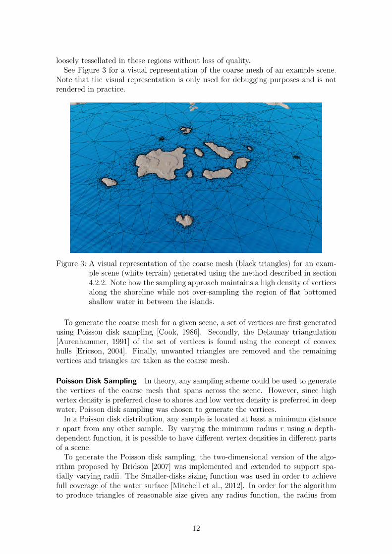
loosely tessellated in these regions without loss of quality.See Figure 3 for a visual representation of the coarse mesh of an example scene.

Note that the visual representation is only used for debugging purposes and is notrendered in practice.

Figure 3: A visual representation of the coarse mesh (black triangles) for an exam-ple scene (white terrain) generated using the method described in section4.2.2. Note how the sampling approach maintains a high density of verticesalong the shoreline while not over-sampling the region of flat bottomedshallow water in between the islands.

To generate the coarse mesh for a given scene, a set of vertices are first generatedusing Poisson disk sampling [Cook, 1986]. Secondly, the Delaunay triangulation[Aurenhammer, 1991] of the set of vertices is found using the concept of convexhulls [Ericson, 2004]. Finally, unwanted triangles are removed and the remainingvertices and triangles are taken as the coarse mesh.

Poisson Disk Sampling In theory, any sampling scheme could be used to generatethe vertices of the coarse mesh that spans across the scene. However, since highvertex density is preferred close to shores and low vertex density is preferred in deepwater, Poisson disk sampling was chosen to generate the vertices.

In a Poisson disk distribution, any sample is located at least a minimum distancer apart from any other sample. By varying the minimum radius r using a depth-dependent function, it is possible to have different vertex densities in different partsof a scene.

To generate the Poisson disk sampling, the two-dimensional version of the algo-rithm proposed by Bridson [2007] was implemented and extended to support spa-tially varying radii. The Smaller-disks sizing function was used in order to achievefull coverage of the water surface [Mitchell et al., 2012]. In order for the algorithmto produce triangles of reasonable size given any radius function, the radius from

12

the function is clamped so that it lies within a fixed range [rmin, rmax]. Clampingthe radius in this manner also lets the algorithm terminate in a reasonable amountof time.

Bridson’s algorithm takes the extents of the sample domain and the minimumradius r as parameters and produces a Poisson disk sampling in linear time. First, abackground grid with cell size equal to r/

√2 is initialized to accelerate neighborhood

searches. An initial sample is randomly picked from the sample domain and insertedinto the background grid and into an active list. While the active list is not empty,a random point p is picked from it and k new candidate points are generated ina circular annulus between r and 2r around p. For each candidate point, the 9neighboring background grid cells are checked for a potential overlap with an existingsample. If a candidate point does not violate the circular area of radius r aroundany existing sample, the candidate becomes a new sample and is added to thebackground grid and active list. In practice, k = 30 worked well.

The algorithm was extended to support spatially varying radii by introducinga radius function r = f(~x). The background grid must now have a cell size ofrmin/

√2 to avoid conflicts. The Smaller-disks sizing function accepts a candidate

point if the distance between it and any existing sample is less than the minimumof f(candidate point) and f(sample point)).

The obvious problem with this extension is that the worst case number of neigh-boring background grid cells to check increases dramatically. However, it did notprove to be a problem in practice.

Next, the radius function must be chosen. If the radius function is made propor-tional to the water depth h, the density of the generated points will increase as thedepth decreases:

r = k |h| ,

where k is a user defined constant. Negative depth values occur where the terrainof the scene is above the water surface and taking the absolute value makes thesampling symmetric with respect to the shoreline. Coarse mesh vertices are neededon both sides of the shoreline in order for coarse mesh triangles to cover the spaceup to the very start of the terrain. Choosing k = 1 is reasonable and will producepoints approximately 1 unit apart at a depth of 1 unit. A problem with this samplingapproach is that it generates too many points in large areas of shallow water wherethe seabed is nearly flat. Since a low number of coarse mesh triangles is critical forperformance in the rendering step, the sampling approach must be improved.

The observation that an initially straight wavefront will remain straight when ittravels in an area of uniform depth can be used to construct a sampling in a similarway: The radius function can be made proportional to the inverse length of thegradient at the candidate point:

r =k

max(ε, |∇h|),

where ε is a small number that determines the size of the largest triangle andprevents division by zero. With this approach, it is important that the underlying

13

depth field is smooth and does not contain too high-frequency features. In practice,this is achieved by the relatively sparse terrain representation described in 4.2.1.This sampling approach eliminates the high point density in shallow waters wherethe seabed is nearly flat but it also disregards the shoreline and nearly flat bottomedshores are sampled sparsely. Shores need to be sampled densely no matter thegradient in order for the simulation to accurately capture wave reflections. Thus,the sampling approach needs to be improved further.

A good radius function was achieved by combining the two sampling approachesinto one:

r =k |h|

max(ε, |∇h|)

With this sampling approach, shores are sampled densely and flat bottomed shal-low waters are sampled sparsely, as desired (See Figure 3). In practice, k = 1 andε = 0.1 was found to be suitable for scenes where 1 world unit corresponds to 1meter.

Delaunay Triangulation In order to create the coarse mesh triangles, the Delaunaytriangulation of the coarse mesh vertices is computed. The Delaunay triangulationmaximizes the minimum interior angle of all triangles in the triangulation.

The method chosen to compute the Delaunay triangulation takes advantage ofthe fact that there is a connection between the Delaunay triangulation of a setn-dimensional points and the convex hull of the set of points lifted to a n+1-dimensional parabola [Edelsbrunner and Seidel, 1985]. First, the set of 2-dimensionalcoarse mesh vertices are lifted to a 3-dimensional parabola where the third coordi-nate is taken as the squared distance to the origin:

~p =(vx vy v2

x + v2y

)T.

Intuitively, one can think of the points as being placed on the bottom surface of abowl that extends upwards in the positive z-direction and that is placed on a tablemade up of the x and y axis. Next, the convex hull of the set of 3-dimensional pointsis computed. Finally, only the triangles of the convex hull that can be seen froman observer at z = −∞ looking in the positive z-direction are kept, i.e., triangleswhose normals ~n fulfill nz < 0. The 3-dimensional triangles are then projected ontothe original two-dimensional plane by discarding the z-coordinate. This procedureyields the sought after closest-point Delaunay triangulation of the original point set[Edelsbrunner and Seidel, 1985].

By transforming the problem in this way, the focus is shifted from implementing arobust two-dimensional Delaunay triangulation algorithm to implementing a robustthree-dimensional convex hull generation algorithm.

Convex Hull Generation To construct the convex hull of the lifted set of pointsin three dimensions, the algorithm proposed by Gustafsson [2013] was implemented.

14

The algorithm was chosen over other more widespread algorithms because of itssimplicity and promising inherent robustness. As the algorithm is topology-based,it will always produce a two-manifold mesh where every edge belongs to exactlytwo triangles as long as it terminates. However, the algorithm is not guaranteed toterminate due to the limited precision of floating point numbers. Since terminationis crucial in a production environment, the algorithm was extended and made robustat the cost of performance.

Gustafsson’s algorithm is inspired by support mapping methods such as theGilbert-Johnson-Keerthi (GJK) algorithm [Gilbert et al., 1988] in that it uses a

support function to incrementally build the convex hull. Given any direction ~d, thesupport function returns the point in the set that lies furthest in that direction, i.e.,the point ~pi for which ~pi · ~d = max(~p1 · ~d, ~p2 · ~d, . . . , ~pn · ~d) holds. From this followsthat any point returned by the support function lies on the surface of the convexhull of the point-set.

The algorithm starts by using the support function to construct an initial convexhull consisting of two oppositely oriented triangles from 3 points. The rest of thepoints in the input set are added to a remaining point set. In each iteration ofthe algorithm, a triangle is picked from the convex hull and the support functionis queried for the point ~pnew in the remaining point set that lies furthest along thetriangle normal. If ~pnew lies in front of the triangle, the triangle is replaced by 3 newtriangles that connect the edges of the original triangle and ~pnew. The point ~pnew

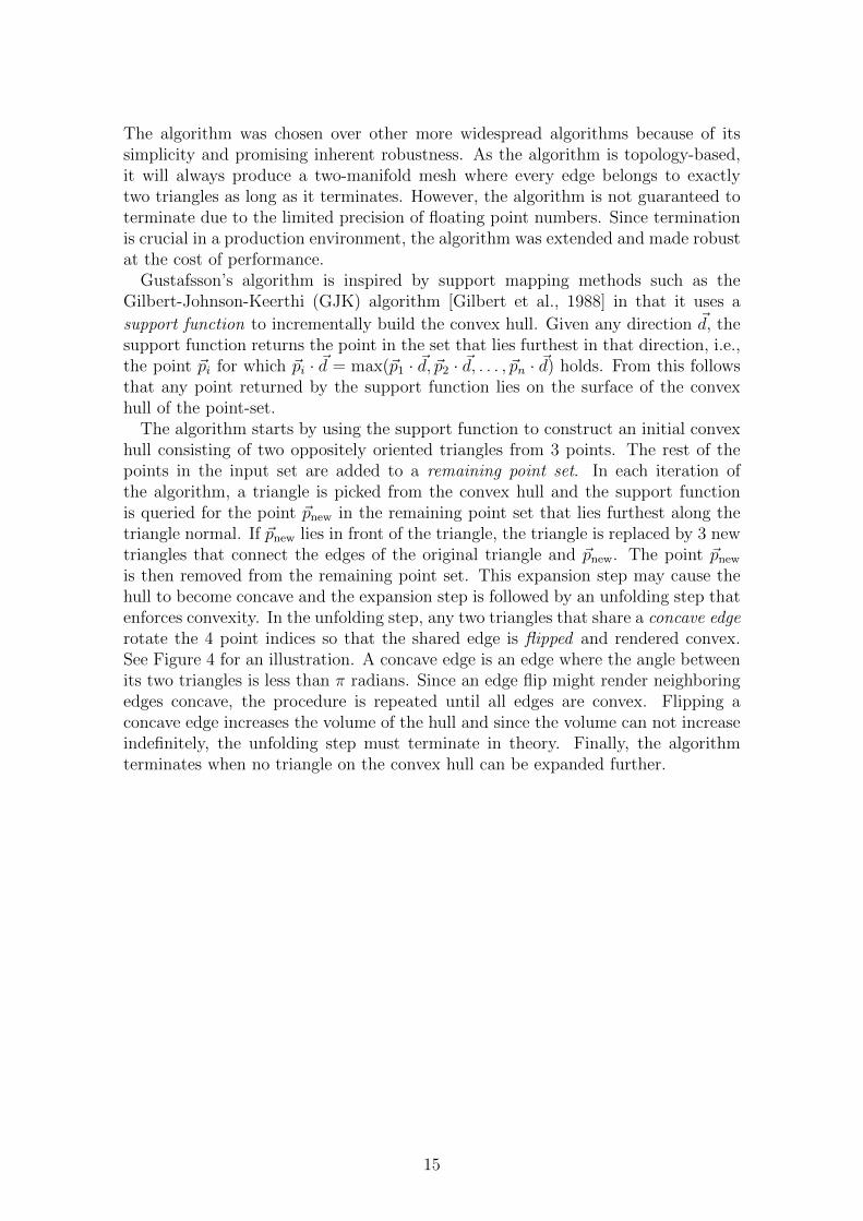
is then removed from the remaining point set. This expansion step may cause thehull to become concave and the expansion step is followed by an unfolding step thatenforces convexity. In the unfolding step, any two triangles that share a concave edgerotate the 4 point indices so that the shared edge is flipped and rendered convex.See Figure 4 for an illustration. A concave edge is an edge where the angle betweenits two triangles is less than π radians. Since an edge flip might render neighboringedges concave, the procedure is repeated until all edges are convex. Flipping aconcave edge increases the volume of the hull and since the volume can not increaseindefinitely, the unfolding step must terminate in theory. Finally, the algorithmterminates when no triangle on the convex hull can be expanded further.

15

A

B

A

(B)

ḇ

ḇ

Flip

Figure 4: A concave edge is flipped by rotating the 4 point indices of the two con-nected triangles in the unfolding step of the convex hull generation al-gorithm. The edge is considered concave when the angle α between thetriangles that share the edge is less than π radians. As seen in the figure,a flip renders a concave edge convex.

In practice, the limited precision of floating point numbers might cause the un-folding step to cycle through a set of flips indefinitely. Indefinite cycling might occurwhenever the concavity tests for a series of edges do not agree about the convexityof the hull and the same edges are repeatedly flipped in some cycle. However, theexact same edge that is part of the exact same two triangles should not be flippedtwice as this will undo the work of the first flip. To make the algorithm robust, thefirst flip is assumed to be correct and a flip hash set is used to store the 4 verticesassociated with each performed flip. At the start of the unfolding step, the flip hashset is initialized to the zero set. Then, whenever a flip is about to be performed, itis first checked against the flip hash set. If there is a match and the flip is aboutto undo the work of a previous flip, the flip is skipped. If not, the concavity test isassumed to be correct and the flip is performed and added to the flip hash set. Asthere is a finite number of possible flips, the extension will allow termination of theunfolding step and make the algorithm robust against precision errors. In practice,the high number of possible flips was not a problem and the algorithm successfullyterminated in a reasonable amount of time even for very large scenes with largevariations in triangle size.

Removal of Hidden Triangles In most scenes, some of the generated triangles ofthe coarse mesh will lie completely below the terrain of the world. As no water willbe visible in these areas, it is unnecessary to store wave data on the triangles.

In order to save memory, the unnecessary triangles are removed from the coarsemesh in a post-processing step. First, all vertices of the coarse mesh that lie be-low the terrain are marked as invisible. Then, all coarse mesh triangles that are

16

connected to only invisible vertices are removed. This simple procedure might re-move partly visible triangles in theory. However, as long as the shoreline was welltessellated it did not prove to be a problem in practice.

4.2.3 Wavefront Generation

In order for the simulation of the water to be realistic and at the same time allowfor artistic control, a flexible system for generating wavefronts must be in place. Asingle virtual scene may contain many different settings in which water should bepresent. There should be large ocean waves at open sea, less violent waves in baysand calm water in canals further inland. There might be waterfalls as a result ofdrops in elevation or man-made construction such as dams. To capture these designgoals, the system provides a set of wavefront generators that can be placed in ascene and allow artists to tailor the scene to their vision.

All wavefront generators let the user specify a minimum and maximum angularfrequency range that the wavefronts created from the generator will be limited to. Agenerator typically creates several wavefronts and the angular frequency value usedfor an individual wavefront is restricted to this range. In addition to the angularfrequency range, a maximum amplitude to wavelength ratio is specified to controlthe maximum steepness of all waves that result from the generator.

Sampling the Ocean Wave Spectrum In order to avoid having an artist specifythe parameters for each wavefront manually in an open sea setting, wavefronts can begenerated by sampling an ocean wave spectrum. The Pierson-Moskowitz spectrum[Pierson and Moskowitz, 1964] is used and extended to two dimensions using asimple falloff function that eliminates waves perpendicular to the wind direction.Two integer values denote the number of angular frequency samples and the numberof directional samples respectively.

In contrast to Frechot [2006] that use an adaptive sampling scheme to finely sampleareas of high wave energy, a good range of angular frequencies is preferred whengenerating wavefronts. Thus, a simple uniform sampling scheme is used. A set ofdensities are computed by sampling the spectrum using a jittered regular grid in theangular frequency/wind angle plane. When sampling the wave spectrum, the densityis discretized and converted to wave amplitude as shown by Frechot [2006]. Thenfor each sample, a wavefront is created (with the corresponding angular frequency,propagation direction and amplitude) and spawned just outside the bounds of thewater simulation area.

Manual Placement of Wavefronts To allow fine grain control over waves in aparticular location, the system provides a planar wavefront generator and a circularwavefront generator. The planar wavefront generator creates a number of wavefrontsthat lie parallel to the x-axis and at the position of the generator entity. The circularwavefront generator creates a number of circular wavefronts around the position ofthe generator entity.

Both of these generators let the user specify a minimum and maximum energyrange and the number of wavefronts to create. The energy range must be within

17

[0, 1] and denotes the amplitude from zero to maximum steepness as dictated by themaximum amplitude to wavelength ratio. For each wavefront, an angular frequencyvalue is uniformly sampled from the angular frequency range and an energy value isuniformly sampled from the energy range. Then, the amplitude of the wavefront isdetermined by multiplying the initial wavelength of the wavefront with the maximumamplitude to wavelength ratio and the sampled energy value.

4.2.4 The Wavefront

In the simulation step, a wavefront is represented by a list of n vertices and a listof n − 1 line segments. The vertices and line segments form a curve on the watersurface and describe the current shape and location of the wavefront in world space.The resolution of the wavefront changes as the wavefront is propagated across thewater surface [Vinje et al., 1993, Gonzato and Le Saec, 2000, Jeschke and Wojtan,2015] in order for the piecewise linear representation to approximate the true shapeof the wavefront even as it deforms considerably. See Table 1 for what is stored inmemory for each wavefront.

WavefrontProperty Symbol TypeAngular Frequency ω FloatPhase φ FloatPrevious Phase φ′ FloatVertices N/A Vertex[ ]Segments N/A Segment[ ]Covered Mesh Edges N/A MeshEdge{ }Initial Amplitude/Wavelength Ratio N/A FloatMin Amplitude/Wavelength Ratio N/A FloatMax Amplitude/Wavelength Ratio N/A FloatMax Amplitude/Depth Ratio N/A Float

Table 1: The Wavefront Data Structure

The Angular Frequency and Phase are the parameters of the wave that areshared across all vertices and segments of the wavefront. Waves with an ampli-tude/wavelength ratio below Min Amplitude/Wavelength Ratio are not visible andshould be removed. As the simulation does not capture non-linear effects of wa-ter behavior, such as breaking waves, the amplitudes of the segments are simplyclamped to lie just below the breaking point of the wave using the Max Ampli-tude/Wavelength Ratio value. In a similar fashion, Max Amplitude/Depth Ratio isused to clamp the amplitudes of segments that exceed the current water depth. TheInitial Amplitude/Wavelength Ratio is used to compute the initial amplitude of thesegments of a wavefront when the wavefront is manually placed within a scene asrandom uniform sampling of this value gives much more believable wave profilesthan random uniform sampling of the amplitude directly. This parameter is notused when the wavefront is generated from an ocean wave spectrum.

18

The integration scheme proposed by Jeschke and Wojtan [2015] was adopted andused to deduce the vertex and segment data structures. In addition to its currentstate, each vertex and segment also stores some of its previous state so that certainvalues can be interpolated between time steps when the wavefront is recorded ontothe coarse mesh. See Table 2 and Table 3 for what is stored in memory for eachvertex and each segment respectively.

VertexProperty Symbol TypePosition ~p (Float, Float)

Normalized Travel Direction ~d (Float, Float)Depth Below Surface h FloatWavenumber k FloatPhase Speed c FloatGroup Speed cg Float

Previous Position ~p′ (Float, Float)

Previous Normalized Travel Direction ~d′ (Float, Float)Previous Wavenumber k′ FloatPrevious Phase Speed c′ FloatPrevious Group Speed c′g FloatWithin Bounds Flag N/A BooleanMoving Away Flag N/A BooleanReflection Depth N/A Integer

Table 2: The Vertex Data Structure

SegmentProperty Symbol TypeAmplitude a FloatEnergy Respecting Amplitude aD FloatPrevious Amplitude a′ FloatPrevious Energy Density D′ FloatPrevious Length L′ FloatDegenerate Flag N/A BooleanInverted Amplitude Flag N/A Boolean

Table 3: The Segment Data Structure

The division of wave parameters between Vertex and Segment where made tofacilitate the integration scheme described in section 4.2.6.

The Within Bounds Flag and Moving Away Flag are used to keep track of wherea vertex is in relation to the extents of the water surface. If a vertex is not withinbounds and it is moving away, it is removed from the simulation. The ReflectionDepth value counts the number of times a vertex has been reflected off the shore andis analogous to the recursion depth value used in conventional ray tracing of lightrays for image generation. The Degenerate Flag is used to denote segments that are

19

no longer a good fit for the simulation and are about to be removed. The InvertedAmplitude Flag is used to keep track of the sign of the amplitude of a segment. Anexplicit flag makes computations involving amplitude and energy density simplerand results in more readable code.

4.2.5 The Simulation Step

The simulation step propagates the wavefronts across the water surface and recordswave data onto the coarse mesh whenever a wavefront segment passes over a coarsemesh vertex. The wave data samples are connected by chains stored on the coarsemesh edges. When all wavefronts have been propagated, the chains are combinedinto wave overlaps stored on the coarse mesh triangles. Finally, the coarse meshtriangles form the coarse mesh that is used as the input to the rendering step.

The simulation follows a simple procedure:

1. Propagate wavefronts forward in time

2. Record wavefronts onto coarse mesh

3. If no wavefronts are left, end the simulation; otherwise return to step 1

The propagation step is described in Section 4.2.6 and the recording step is de-scribed in Section 4.2.8.

4.2.6 Wavefront Propagation

The wavefront propagation step consists of the following 12 sub-steps. Each wave-front in the simulation is handled, in order, within each sub-step.

1. Clean up covered edges

2. Remove degenerate segments

3. Maintain wavefront resolution

4. Compute wavenumbers

5. Conserve energy

6. Compute phase speeds

7. Handle refraction

8. Integrate position

9. Check within bounds

10. Compute depths

11. Handle reflection

12. Identify degenerate segments

The remainder of this section describe the details necessary to robustly implementthe wavefront propagation.

20

Clean up covered edges Each wavefront stores the set of coarse mesh edges thatit covers at any given movement. A wavefront covers a coarse mesh edge if any ofits segments intersect the edge.

In this step, the set of covered edges is iterated and any edge the wavefront nolonger covers is removed from the set.

Remove degenerate segments This step iterates the list of segments and removesall segments that are marked as degenerate. A segment is marked as degenerate inthe Identify degenerate segments step and may become degenerate for a numberof different reasons. For example, any segment that moves away from the watersimulation area is marked as degenerate.

If a wavefront does not contain any segment after this step, it is removed fromthe simulation.

Maintain wavefront resolution In order to reliably simulate a wavefront, a con-stant spatial resolution must be enforced as it is propagated across the scene. If theresolution is insufficient, the piecewise linear representation will poorly represent thetrue shape of the wavefront.

Previous simulation methods keep the resolution constant in world space [Gonzatoand Le Saec, 1997]. This works well for slowly expanding or contracting wavefrontswhere neighboring vertices are moving in roughly the same direction. However, asthe method does not take the curvature of the wavefront into account, it performspoorly when there are sharp changes in travel direction or kinks in the wavefront.In such cases, the wavefront will be under-sampled and its motion unpredictable.

A common problematic case is when an initially straight wavefront develops aswallowtail pattern as it passes through a local low speed region (See Figure 2). Inthis case, two kinks will develop on either side of the slow moving center-sectionof the wavefront as the outer edges fold over it. There will be large differences inthe travel direction of neighboring vertices that lie on either side of a kink, and thesharp corner will be poorly represented if the resolution is held constant in worldspace.

To solve the problem, the observation that a wavefront with kinks in world spacebecomes a smooth bicharacteristic strip when it is transformed into reduced phasespace [Osher et al., 2002, Hauser et al., 2006] is used and the wavefront resolution isheld constant in reduced phase space. See Figure 5 for an illustration of a wavefrontin world space and its corresponding shape in reduced phase space.

21

y

x

xRPS

z

Figure 5: An illustration of a wavefront in world space (dark gray curve) and itscorresponding shape in reduced phase space (red curve). Note that thewavefront does not self-intersect nor display kinks in reduced phase space.

First, each vertex position ~x is lifted to reduced phase space:

~xRPS =(xx xy α arccos(dx) sign(dy))

)T,

where α is a normalizing scaling factor and

sign(x) =

{1 x ≥ 0

−1 x < 0.

Then, for each segment, the minimum distance between its 2 vertices in three-dimensional reduced phase space is determined while taking the periodicity of thez-coordinate into account.

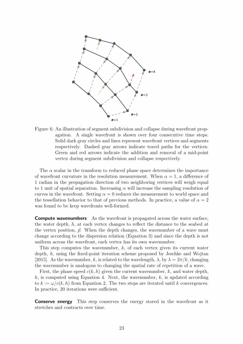
Let δ denote the ideal world space distance between wavefront vertices. If thelength of a segment in reduced phase space is larger than 1.5 δ, the segment issubdivided to two segments by inserting a mid-point vertex. If the segment lengthin reduced phase space is below 0.5 δ, it is collapsed and the two vertices makingup the segment are replaced with a mid-point vertex. The collapse removes theoriginal segment and connects its two adjacent segments together. In both cases,linear interpolation is used to generate the state of the new vertex. See Figure 6 foran illustration of segment subdivision and collapse.

22

Ḽ=1Ḽ=2

Ḽ=3

Ḽ=4

Figure 6: An illustration of segment subdivision and collapse during wavefront prop-agation. A single wavefront is shown over four consecutive time steps.Solid dark gray circles and lines represent wavefront vertices and segmentsrespectively. Dashed gray arrows indicate travel paths for the vertices.Green and red arrows indicate the addition and removal of a mid-pointvertex during segment subdivision and collapse respectively.

The α scalar in the transform to reduced phase space determines the importanceof wavefront curvature in the resolution measurement. When α = 1, a difference of1 radian in the propagation direction of two neighboring vertices will weigh equalto 1 unit of spatial separation. Increasing α will increase the sampling resolution ofcurves in the wavefront. Setting α = 0 reduces the measurement to world space andthe tessellation behavior to that of previous methods. In practice, a value of α = 2was found to be keep wavefronts well-formed.

Compute wavenumbers As the wavefront is propagated across the water surface,the water depth, h, at each vertex changes to reflect the distance to the seabed atthe vertex position, ~p. When the depth changes, the wavenumber of a wave mustchange according to the dispersion relation (Equation 3) and since the depth is notuniform across the wavefront, each vertex has its own wavenumber.

This step computes the wavenumber, k, of each vertex given its current waterdepth, h, using the fixed-point iteration scheme proposed by Jeschke and Wojtan[2015]. As the wavenumber, k, is related to the wavelength, λ, by λ = 2π/k, changingthe wavenumber is analogous to changing the spatial rate of repetition of a wave.

First, the phase speed c(k, h) given the current wavenumber, k, and water depth,h, is computed using Equation 4. Next, the wavenumber, k, is updated accordingto k := ω/c(k, h) from Equation 2. The two steps are iterated until k convergences.In practice, 20 iterations were sufficient.

Conserve energy This step conserves the energy stored in the wavefront as itstretches and contracts over time.

23

First, the group speed, cg, of each vertex is approximated by finite differences ofEquation 3:

cg :=ω(k + ∆k, |h|)− ω(k, |h|)

∆k,

with ∆k = 10−4.Then, the segments are updated in the following manner: First, the current and

previous group speed of the segment, cg and c′g, is computed by averaging the groupspeeds of the two vertices. Second, the world-space length L of the segment isdetermined. Third, the energy density is computed:

D :=c′gcg

L′

LD′.

Fourth, the wavenumber of the segment, k, is computed by averaging the wavenum-ber of the two vertices. Fifth, the amplitude is calculated:

a :=

√2D

ρg + σk2.

Finally, the wavelength of the segment, λ = 2π/k, is multiplied with the MaxAmplitude/Wavelength Ratio and the average depth of the two vertices, h, is mul-tiplied with the Max Amplitude/Depth Ratio in order to yield amax steepness andamax depth respectively. If a > amax steepness, the waves are steep enough to breakand should tumble over themselves in a non-linear fashion in order to dissipate en-ergy. However, as the simulation is based on linear wave theory that is not able tocapture this phenomenon, energy is simply removed from the simulation by settinga := amax steepness and recalculating the energy density using Equation 6. At thispoint, the Energy Respecting Amplitude is set to the current amplitude aD := a.Next, if a > amax depth, the wave will with high probability contribute to bring thewater surface down below the seabed when the water is rendered. As this is likelya temporary problem caused by a sudden spike in the underlying terrain height,the energy density is left unchanged and only the amplitude is clamped by settinga := amax depth. This behavior is not realistic but it increases the lifetime of thewavefronts and lets them reach further inland while preventing the resulting wavesfrom intersecting the terrain, which increases the overall perceived quality of thesimulation.

Note that the amplitude is calculated from the energy density each time step andonly used when the wavefront is recorded onto the coarse mesh. Thus, clamping theamplitude does not influence the future of the simulation.

Compute phase speeds In this step, the phase speed c of each vertex is updatedaccording to Equation 2, c = ω/k, where ω is the angular frequency of the wavefrontand k the most recent wavenumber of the vertex.

Note that this is the analytical phase speed c(k, h) computed in the last iterationof the fixed-point iteration scheme in the Compute wavenumbers step.

24

Handle refraction In order to capture wave refraction, wavefront vertices refractas they pass contour lines in the underlying water depth field [Fournier and Reeves,1986, Ts’o and Barsky, 1987, Gonzato and Le Saec, 1997, Jeschke and Wojtan,2015].

The gradient of the seabed, ∇h, is evaluated at the position of each vertex. If|∇h(~p)| > 10−2, Snell’s law is used with the previous phase speed, c′, and the newphase speed, c, to determine the new propagation direction of the vertex:

~d :=

{~n√

1− s2 + ~t s |s| ≤ 1~d− 2(~d · ~n)~n |s| > 1

,

where

~n =

{∇h(~p)/|∇h(~p)| ~d · ∇h(~p) ≥ 0

−∇h(~p)/|∇h(~p)| ~d · ∇h(~p) < 0,

~t =(−ny nx

)T,

s =c

c′~d · ~t.

Note that the normal ~n always point in the direction of ~d and that ~d is reflectedalong ~n if total internal reflection occurs (|s| > 1).

Integrate position In this step, the vertex positions are integrated forward in timeusing simple Euler integration:

~p := ~p′ + ~d c∆t.

More advanced integration schemes could be used but Euler integration provedto work well in practice.

Check within bounds Since the vertices have been moved to new locations in theprevious step, their state flags must now be updated.

Each vertex position is checked against the two-dimensional oriented boundingbox of the focus area. The focus area is a part of the water surface in which onewould like the wavefronts to start refract due to changes in depth. Outside the focusarea, waves are assumed to be deep water waves. If no focus area is desired, theoriented bounding box of the focus area is set to that of the whole water surface.

The Within Bounds Flag is set to true if the vertex is inside the oriented boundingbox. The Moving Away Flag is set to true if the vertex is not within bounds andits direction is pointing away from the oriented bounding box.

25

Compute depths In this step, the water depth, h, of each vertex is updated. Inorder for newly created wavefronts to hold their shape until they have entered thesimulation area, the evaluation of water depth depends on the state flags of thevertices. The update is performed in two passes.

In the first pass, the water depth, h, is updated for all vertices that are withinbounds, i.e., whose Within Bounds Flag is set to true. For a given vertex, the worldis queried for the water depth, h, at ~p.

In the second pass, vertices that are not within bounds are considered. For eachsuch vertex, the water depth, h, is set to that of the nearest vertex, by index, alongthe wavefront that is within bounds. If no such vertex exists (no vertex on thewavefront is within bounds), the water depth, h, is set to a maximum value thatcorresponds to the depth in deep water, hmax = 102.

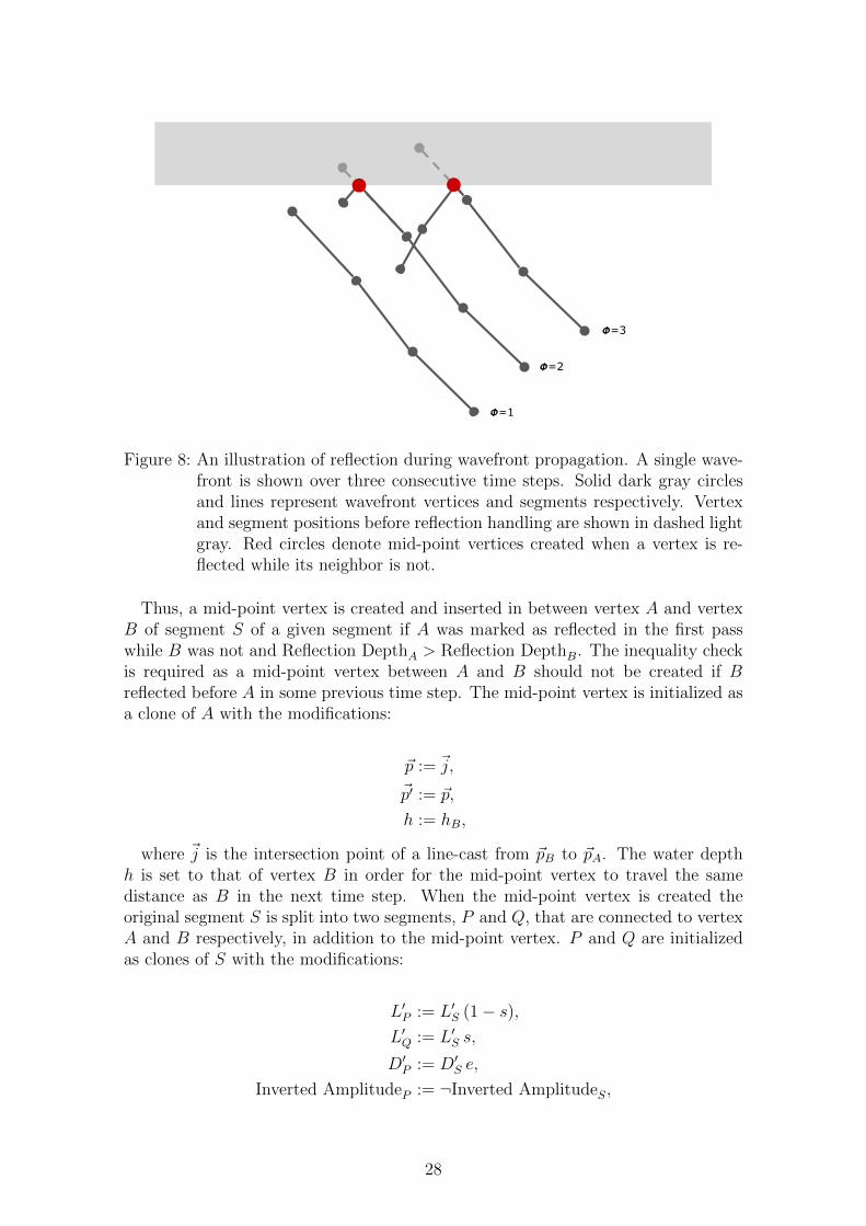
Handle reflection In order to capture waves reflecting off different obstacles in theworld, wavefronts are reflected when they pass the shoreline, defined by h = 0. SeeFigure 7 for an image of a wavefront reflecting off the shoreline in the simulation.

Figure 7: A wavefront reflecting off the shoreline within the simulation. Multipletime steps of the wavefront are shown transitioning from green to red withincreasing phase. The coarse triangle mesh is shown in black. Underneath,the resulting water surface produced by the rendering step is shown in blue.

In order to limit the number of wavefronts and improve performance of the simu-lation and rendering step, each vertex keeps an internal counter of how many timesit has reflected and loses its ability to reflect once the counter exceeds a set limit.In practice, the limit was set to 6 reflection bounces.

The reflection handling is performed in two passes. In the first pass, all verticesof the wavefront are iterated. The position ~p and the position in the previous timestep ~p′ are used as arguments in a line-cast query of the world. If the line intersectsthe shoreline, the vertex is temporarily marked as reflected and updated with:

26

~prefl := ~p− 2((~p−~i) · ~n)~n,

~drefl := ~d− 2(~d · ~n)~n,

~p′refl :=~i,

~d′refl := ~drefl,

hrefl := h(~i),

Reflection Depthrefl := Reflection Depth + 1,

where~i and ~n is the intersection point and normal of the line-cast. Internally, thenormal is set to the normalized gradient of the terrain at the point of intersection,~n = ∇h(~i)/|∇h(~i)|.

In the second pass, mid-point vertices are inserted between segment vertex pairsin which one of the vertices reflects while its neighbor does not in order to betterrepresent the kink in the wavefront that appears in such cases. See Figure 8 for anillustration. The mid-point vertices created during one time step should separatethe wavefront into partitions in which the Reflection Depths of the vertices are equaland distinct from the vertices of neighboring partitions. If a single mid-point vertexis created during one time step, all vertices to the right of this vertex will havereflected one more time than the vertices to the left of it, or vice versa depending onfrom which direction the wavefront hit the shoreline. As the amplitudes of reflectingwaves are inverted and the mid-point vertices split each segment that intersects theshoreline into two new segments (that lie on either side of the intersection), they alsoserve the purpose of clearly defining which segments should have their amplitudeinverted.

27

=1

=2

=3

Figure 8: An illustration of reflection during wavefront propagation. A single wave-front is shown over three consecutive time steps. Solid dark gray circlesand lines represent wavefront vertices and segments respectively. Vertexand segment positions before reflection handling are shown in dashed lightgray. Red circles denote mid-point vertices created when a vertex is re-flected while its neighbor is not.

Thus, a mid-point vertex is created and inserted in between vertex A and vertexB of segment S of a given segment if A was marked as reflected in the first passwhile B was not and Reflection DepthA > Reflection DepthB. The inequality checkis required as a mid-point vertex between A and B should not be created if Breflected before A in some previous time step. The mid-point vertex is initialized asa clone of A with the modifications:

~p := ~j,

~p′ := ~p,

h := hB,

where ~j is the intersection point of a line-cast from ~pB to ~pA. The water depthh is set to that of vertex B in order for the mid-point vertex to travel the samedistance as B in the next time step. When the mid-point vertex is created theoriginal segment S is split into two segments, P and Q, that are connected to vertexA and B respectively, in addition to the mid-point vertex. P and Q are initializedas clones of S with the modifications:

L′P := L′S (1− s),L′Q := L′S s,

D′P := D′S e,

Inverted AmplitudeP := ¬Inverted AmplitudeS,

28

where

s =

{|(~j − ~pB)|/|(~pA − ~pB)| index of A is less than index of B

|(~j − ~pA)|/|(~pA − ~pB)| otherwise

and e is a constant scalar in the range [0, 1] denoting the amount of energy notlost in the collision. In practice, e = 0.8 was used.

If both A and B were marked as reflected in the first pass, the geometry of thewavefront is unchanged and S is updated with:

D′S := D′S e,

Inverted AmplitudeS := ¬Inverted AmplitudeS.

Identify degenerate segments In this step, the segments are iterated and degen-erate segments are identified. There are three reasons for which a segment may beflagged as degenerate. If any of them are true, the Degenerate Flag of the segmentis set to true.

First, a segment is marked as degenerate if the wave generated by the segmentis not steep enough, i.e., if aD/λA < Min Amplitude/Wavelength Ratio ∨ aD/λB <Min Amplitude/Wavelength Ratio is true where λA = 2π/kA and λB = 2π/kB arethe wavelengths of the two vertices of the segment. Note that this is the samesteepness measurement as used in the Conserve energy step. Waves that are deemednot steep enough have an unperceivable effect on the final water surface and theremoval of these segments is crucial for good performance of both the simulationand rendering step. In practice, Min Amplitude/Wavelength Ratio = 5 · 10−3 wasused.

Secondly, a segment is marked as degenerate if both of its vertices have left thewater simulation area and are moving away, i.e., if Moving Away FlagA ∧Moving Away FlagB is true.

Thirdly, a segment is marked as degenerate if any of its vertices are below theterrain of the world, i.e., if hA < −ε ∨ hB < −ε is true and ε is a small positivevalue to account for floating-point precision errors in the Handle reflection step. Inpractice, ε = 10−2 was used.

4.2.7 The Chain

In the recording step, wave data samples are recorded onto the coarse mesh inchains stored on coarse mesh edges. Whenever a wavefront segment passes a coarsemesh vertex, a wave data sample is constructed and a chain referencing this sampleis created and added to each edge connected to the vertex. A sample stores asnapshot of the phase, amplitude, phase speed and normalized travel direction ofthe wavefront as it moved past the vertex. A chain stores the extent of a wavefrontthat has moved past an edge and is used to connect samples that may be safelyinterpolated along edges. A chain can have up to two samples associated with it.

29

See Table 4 and Table 5 for what is stored in memory for each sample and eachchain respectively.

SampleProperty TypeVertex PointerPhase FloatAmplitude FloatPhase Speed FloatNormalized Travel Direction (Float, Float)

Table 4: The Sample Structure

ChainProperty TypeWavefront PointerLeft Vertex Index IntegerRight Vertex Index IntegerSample Count IntegerSample 0 SampleSample 1 SampleSide Of Edge Determined Flag BooleanSide Of Edge Positive Flag Boolean

Table 5: The Chain Structure

Let a vertex vi on a wavefront be covered by a chain if the chain’s Wavefrontpointer references the wavefront and Left Vertex Index ≤ i ≤ Right Vertex Index.A determined chain is a chain in which all wavefront vertices covered by the chainare located on one side of the line spanned by the coarse mesh edge the chain belongsto. Determined chains are usually created if the wavefront is parallel to the coarsemesh edge as the chain is created. An undetermined chain is a chain in which atleast two of the wavefront vertices lie on opposite sides of the line spanned by thecoarse mesh edge the chain belongs to. Undetermined chains may be created when awavefront is perpendicular to a coarse mesh edge and a wavefront segment intersectsthe coarse mesh edge as it passes a coarse mesh vertex. As soon as a chain becomesdetermined, the Side Of Edge Determined Flag is set to true and the Side Of EdgePositive Flag is set to true if the covered wavefront vertices lie above the coarsemesh edge, otherwise it is set to false. A point ~p lies above a coarse mesh edge if(~p− ~o) · ~n > 0, where ~n is the counter-clockwise normal of the edge and ~o is a pointon the edge. A point lies on the correct side of a coarse mesh edge with respect toa determined chain if the point lies above the edge and the Side Of Edge PositiveFlag is set to true or if the point does not lie above the edge and the Side Of EdgePositive is set to false. Once a chain has been determined its flags are fixed and thechain cannot become undetermined or change side unless it is merged with anotherchain.

30

When a chain with at least one sample associated with it is removed from a coarsemesh edge, it is saved in a list of finished chains that are stored on the edge. It iscrucial to save all chains that contain samples, no matter the situation in which theyare removed, since there are always several chains being created (on multiple coarsemesh edges) referencing the same sample and if any single one of them is savedwhile another is not, there will be a discontinuity in the water surface. Finishedchains are immutable and are only used as input to the final step of the coarse meshconstruction procedure where they are combined into wave overlaps, as described inSection 4.2.9.

4.2.8 Wavefront Recording

The wavefront recording step consists of the following 6 sub-steps. Each wavefrontin the simulation is handled, in order, within each sub-step.

1. Update map of all covered edges

2. Validate existing chains

3. Create new chains

4. Expand determined chains

5. Merge overlapping chains

6. Remove finished chains

See Figure 9 for an overview of the whole procedure. The remainder of this sectiondescribe the details necessary to robustly record wavefronts.

(a) Create new chain (b) Expand determined chain

(c) Create new chain (d) Expand determined chains

Figure 9: An overview of how chains are used to track a wavefront across a coarsemesh edge over two consequtive time steps.

31

Update map of all covered edges As the later steps are based on manipulatingthe chains of the coarse mesh edges, a map of all edges currently covered by anywavefront is constructed by taking the union of the Covered Mesh Edges sets of allwavefronts.

Validate existing chains In this step, the chains of all covered edges are updatedso that they respect the current state of the wavefronts in the scene.

First, the Left Vertex Index and Right Vertex Index of all chains are clampedto lie within the range of the vertices of the respective wavefront. Secondly, allundetermined chains are tested to see if they qualify as determined chains. Anychain that qualifies as determined is made determined as described in Section 4.2.7.Thirdly, the covered vertex range of each determined chain is shrunk, if possibleand by one vertex at a time, until all covered vertices are on the correct side of thecoarse mesh edge. At last, all determined chains that do not lie on the correct sideof the coarse mesh edge are removed.

Create new chains As the positional update of the wavefronts is discrete, thewavefront recording step must determine if a wavefront passes over any coarse meshvertex as it is swept from its configuration in the previous time step to its configu-ration in the current time step.

Inverse bilinear interpolation [Quilez, 2010] is used to test if a segment overlaps acoarse mesh vertex. If an overlap is found, a sample is created and the coefficients sand t of the inverse bilinear interpolation are used to interpolate the values for thesample from the two time steps of the segment. Then, for each coarse mesh edgeconnected to the overlapped vertex, a chain referencing the new sample is created.See Figure 10 for an illustration of the creation of a chain for a single coarse meshedge.

32

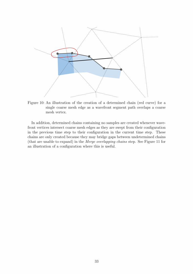
Figure 10: An illustration of the creation of a determined chain (red curve) for asingle coarse mesh edge as a wavefront segment path overlaps a coarsemesh vertex.

In addition, determined chains containing no samples are created whenever wave-front vertices intersect coarse mesh edges as they are swept from their configurationin the previous time step to their configuration in the current time step. Thesechains are only created because they may bridge gaps between undetermined chains(that are unable to expand) in the Merge overlapping chains step. See Figure 11 foran illustration of a configuration where this is useful.

33

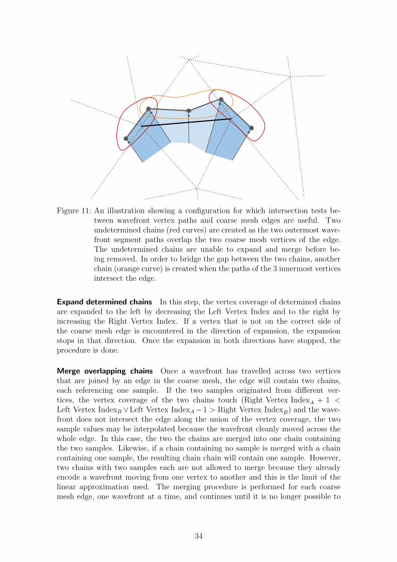
Figure 11: An illustration showing a configuration for which intersection tests be-tween wavefront vertex paths and coarse mesh edges are useful. Twoundetermined chains (red curves) are created as the two outermost wave-front segment paths overlap the two coarse mesh vertices of the edge.The undetermined chains are unable to expand and merge before be-ing removed. In order to bridge the gap between the two chains, anotherchain (orange curve) is created when the paths of the 3 innermost verticesintersect the edge.

Expand determined chains In this step, the vertex coverage of determined chainsare expanded to the left by decreasing the Left Vertex Index and to the right byincreasing the Right Vertex Index. If a vertex that is not on the correct side ofthe coarse mesh edge is encountered in the direction of expansion, the expansionstops in that direction. Once the expansion in both directions have stopped, theprocedure is done.

Merge overlapping chains Once a wavefront has travelled across two verticesthat are joined by an edge in the coarse mesh, the edge will contain two chains,each referencing one sample. If the two samples originated from different ver-tices, the vertex coverage of the two chains touch (Right Vertex IndexA + 1 <Left Vertex IndexB ∨Left Vertex IndexA−1 > Right Vertex IndexB) and the wave-front does not intersect the edge along the union of the vertex coverage, the twosample values may be interpolated because the wavefront cleanly moved across thewhole edge. In this case, the two the chains are merged into one chain containingthe two samples. Likewise, if a chain containing no sample is merged with a chaincontaining one sample, the resulting chain chain will contain one sample. However,two chains with two samples each are not allowed to merge because they alreadyencode a wavefront moving from one vertex to another and this is the limit of thelinear approximation used. The merging procedure is performed for each coarsemesh edge, one wavefront at a time, and continues until it is no longer possible to

34

merge any two chains.Note that two chains with different notions of ”correct side” may be merged if

the wavefront moves perpendicularly to the coarse mesh edge and zig-zags back andforth before leaving the edge. The notion of correct side is only used to removechains for which the wavefront moves back the same way it came before passinganother coarse mesh vertex.

When two chains A and B are merged, they are replaced with a new chain where

Wavefront := WavefrontA

Left Vertex Index := min(Left Vertex IndexA,Left Vertex IndexB)

Right Vertex Index := max(Right Vertex IndexA,Right Vertex IndexB)

Sample Count := Sample CountA + Sample CountB

Sample 0 :=

Sample 0A Sample CountA = 1

Sample 0B Sample CountA = 0∧Sample CountB = 1

Sample 1 :=

Sample 0B Sample CountA = 1∧

Sample CountB = 1

nothing otherwise

Side Of Edge Determined Flag :=

true (DeterminedA ∧DeterminedB ∧SideA = SideB)∨(DeterminedA ∧ ¬DeterminedB)∨(¬DeterminedA ∧DeterminedB)

false otherwise

Side Of Edge Positive Flag :=

SideA DeterminedA

SideB ¬DeterminedA ∧DeterminedB

false otherwise

Remove finished chains In this step, any chain whose wavefront does not intersectthe respective coarse mesh edge is removed.

4.2.9 Combining Chains on Edges Into Wave Overlaps on Triangles

In order to be able to interpolate sample values across coarse mesh triangles, finishedchains from the edges of a triangle are combined into wave overlaps for that triangle.This is done as single-valued functions along coarse mesh edges are combined intosingle-valued functions within coarse mesh triangles by Jeschke and Wojtan [2015].The finished chains with 1 and 2 samples presented in Section 4.2.8 are equivalentto the incomplete and complete edges described by Jeschke and Wojtan [2015].

See Figure 12 for a graphical explanation of the procedure and Table 6 for whatis stored in memory for each resulting wave overlap.

35

(a) 3 chains with 2 samples each combine into 1 wave overlap

(b) 1 chain with 2 samples and 2 chains with 1 sample eachcombine into 2 wave overlaps

Figure 12: Two cases of how 3 chains from 3 coarse mesh edges can be combinedinto wave overlaps for the coarse mesh triangle. Red arrows denote thenormalized travel direction of the samples that are shared between thechains and indicate how the wavefront moved passed the vertices when thesamples were created. The red x denotes a missing sample. A filled blackcircle indicates that the amplitude from the sample is used for that cornerin the wave overlap. A hollow black circle indicates that an amplitude ofzero is used for that corner in the wave overlap. A dashed line indicatesthat the missing sample is replaced with extrapolated values from theexisting sample in the wave overlap. a) All 3 chains contain 2 sampleseach and reference the same 3 samples, indicating that the wavefrontmoved fully past the triangle. A single wave overlap is recorded. b) 1chain with 2 samples and 2 chains with 1 sample each reference the same2 samples, indicating that the wavefront moved passed only one edgebefore being removed or reflected. Two wave overlaps are recorded.

36

Wave OverlapProperty TypeAngular Frequency FloatPhase Float[3]Amplitude Float[3]Phase Speed Float[3]Normalized Travel Direction (Float, Float)[3]

Table 6: The Wave Overlap Structure

First, wave overlaps that represent wavefronts that moved fully past coarse meshtriangles are created (Figure 12a). For each coarse mesh triangle, all combinationsof 3 chains with 2 samples each from the 3 edges of the triangle are found. A waveoverlap is then created for each combination where the 3 chains share the same 3samples.

Secondly, wave overlaps that represent wavefronts that partially crossed coarsemesh triangles are created (Figure 12b). For each coarse mesh triangle, all combi-nations of 2 chains that were not part of a combination enumerated in the first stepare found. A wave overlap is then created for each combination where a sample isshared by the chains. The amplitude recorded at the shared sample gets transferredto the wave overlap whereas the amplitudes of the other corners are set to 0. Missingsamples are approximated by extrapolating the existing sample.

As coarse mesh triangles share the same coarse mesh edges (and consequentlychains), the generated wave overlaps form a continuous surface function with nodiscontinuities across the entire coarse mesh.

Sorting wave overlaps by wavelength Once all wave overlaps of a coarse meshtriangle have been created, they are sorted by wavelength in descending order. Foreach wave overlap, the wavelength of the wave is determined at each triangle vertex i,λi = 2πci/ω, and the minimum of the three values is used for the sorting comparison.Since the wavelength of the wave can not be more extreme inside the triangle thanat any of its vertices when linear interpolation is employed, the minimum value givesa good measurement of the shortest wavelength across the entire wave overlap.

37

4.3 Rendering

The next section will describe the rendering step and how the simulation data storedin the coarse mesh is used to displace and render the water surface. The focus will beon achieving the best possible performance on current generation graphics hardware.

In order to render the water surface using the graphics card (GPU), the surfacemust be decomposed into a set of triangles. The number of triangles pushed to theGPU will partly determine the performance of the rendering step and excessive useof triangles will leave little computational resources to the rest of the virtual world.In a production environment, the water rendering subsystem cannot use a majorityof the typical 16 ms time budget designated to rendering a single frame (with a 60 Hzupdate frequency target). Thus, care must be taken when constructing the watersurface geometry so that only visible triangles are pushed to the GPU. In addition,the screen space size of the triangles should be approximately constant across thewater surface so that the image quality is uniform across the screen and so that nosingle area of the screen is a computational bottleneck.

The coarse mesh constructed in the simulation step might seem to be a naturalchoice for rendering the water surface. For simplicity and compatibility with theprevious water rendering algorithm used by Frostbite [2017], a world space alignedquadtree was used instead. See Section 7.1 for a discussion on the subject.

4.3.1 Water Surface Geometry

In order to construct the vertices and triangles of the water surface geometry, a worldspace aligned quadtree is adaptively subdivided with respect to the view frustumevery frame. Each leaf node in the tree contains a grid of 162 cells (172 = 289 vertices,2 · 162 = 512 triangles) that are rendered using the unique world-space transformof the leaf node. As the tree is adaptively subdivided, different leaf nodes will havedifferent scales and the resolution of the water surface geometry will vary spatiallyin world space. See Figure 13 for an abstract illustration of the tree generation.

38

Figure 13: An illustration of the world space aligned quadtree, as seen from above,that is used to generate the water surface geometry. The view frustum isshown in red and the leaf nodes of the quadtree as gray boxes. Note thatthere are leaf nodes at different spatial scales which gives rise to spatiallyvarying resolution of the water surface.

A node in the tree is subdivided if the world space size of a triangle is largerthan the approximate world space size, in the horizontal or vertical direction, ofrmin pixels at the same distance from the camera. In practice, rmin = 4 pixels wasused which yields surface triangles no larger than 4 pixels in screen space. When nonode of the quadtree can be subdivided further, the resulting vertices and trianglesof the leaf nodes form a flat, adaptively tessellated, water surface across the virtualscene.

The world space aligned quadtree was chosen over a projected grid [Johansonand Lejdfors, 2004] approach because of its inherent spatial persistency. In a worldspace quadtree, it is probable that a vertex on the water surface exists in multiplesubsequent frames of an animation, even if the view frustum is moving, and thiscoherency can be used to optimize the height-lookup of the water surface.

In contrast, when using a projected grid, the positions of vertices projected ontothe water surface are very sensitive to movement of the view frustum and there isno coherency in world space vertex positions between frames. Furthermore, if theprojected grid is not very finely tessellated, movement of the view frustum can causerolling motions on the water surface as the sampling points move in world space,even if the Nyquist limit is respected.

See Figure 14 for a wireframe view of the resulting water surface.

39

(a) rmin = 16

(b) rmin = 4

Figure 14: A wireframe view of the generated water surface. The structure of theworld space aligned quadtree can be seen where there is a resolutiondifference between adjacent leaf nodes, i.e., where leaf nodes at differenttree depths are adjacent. Note that the vertical component of the screenspace triangle size is very small in the distance due to the square node-based subdivision scheme employed. See Section 6 for a discussion on thesubject.

40

4.3.2 Evaluating The Simulation

The next step is to evaluate the simulation by offsetting the vertices on the watersurface according to the wave overlaps stored on the coarse mesh triangles. Com-puting the vertex offset of a single vertex according to the simulation is denoted aheight-lookup. Once the entire water surface has been evaluated for a given anima-tion frame, the water surface can be rendered.

The simplest way of evaluating the simulation for a given animation frame is toperform height-lookups for all vertices in all leaf nodes of the quadtree at once.However, because of the high number of total vertices on the water surface andthe high number of wave overlaps required to reach the desired level of quality,this update scheme is too performance intensive to be used in practice on currentgraphics hardware.

Staggered update scheme To improve performance, the vertices of the watersurface are evaluated using a staggered update scheme at a low update frequency.A staggered update scheme reduces the number of vertices that need to be updatedevery frame by evaluating different vertices every frame according to some pre-defined pattern.

As the simulation data stored in the coarse mesh may be evaluated at any point intime for any world space position independently of previous state, a height-lookupcan be performed for any vertex independently of any other vertex on the watersurface. This makes it possible to evaluate vertices in a staggered fashion. Further-more, if the update frequency of the water is lower than the update frequency ofother aspects of the world, for example the physics engine, it is possible evaluateeach vertex at two points in time and then linearly interpolate between the twoheight values in order to fill in the missing frames and give the impression that theentire virtual world is updated at the same rate.

Vertex displacement buffer In order to implement a staggered update scheme,the offset values computed for a set of vertices during a frame must be accessible insubsequent frames when other vertices are evaluated. A persistent vertex displace-ment buffer is used to keep track of the offsets of all vertices on the water surface. Aleaf node that exists for several frames occupies a fixed set of 289 elements, denoteda slot, in the vertex displacement buffer.

After the quadtree is constructed for a given frame, the leaf nodes of the quadtreeare iterated and compared against the leaf nodes of the quadtree of the previousframe. If a new leaf node that did not exist in the previous frame is encountered, itis assigned a free slot in the vertex displacement buffer. If a leaf node that existedin the previous frame no longer exists in the current frame, its slot in the vertexdisplacement buffer is freed and the data stored in the slot remains unused andstagnant until the slot is assigned to a new leaf node.

In addition, the dynamic buffers required to evaluate and render the water surfaceare filled as the list of leaf nodes are iterated.

41

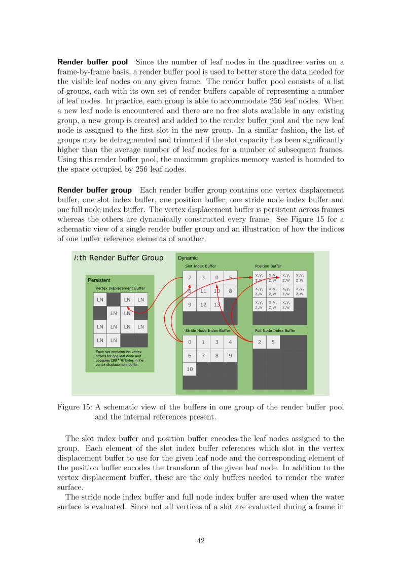
Render buffer pool Since the number of leaf nodes in the quadtree varies on aframe-by-frame basis, a render buffer pool is used to better store the data needed forthe visible leaf nodes on any given frame. The render buffer pool consists of a listof groups, each with its own set of render buffers capable of representing a numberof leaf nodes. In practice, each group is able to accommodate 256 leaf nodes. Whena new leaf node is encountered and there are no free slots available in any existinggroup, a new group is created and added to the render buffer pool and the new leafnode is assigned to the first slot in the new group. In a similar fashion, the list ofgroups may be defragmented and trimmed if the slot capacity has been significantlyhigher than the average number of leaf nodes for a number of subsequent frames.Using this render buffer pool, the maximum graphics memory wasted is bounded tothe space occupied by 256 leaf nodes.

Render buffer group Each render buffer group contains one vertex displacementbuffer, one slot index buffer, one position buffer, one stride node index buffer andone full node index buffer. The vertex displacement buffer is persistent across frameswhereas the others are dynamically constructed every frame. See Figure 15 for aschematic view of a single render buffer group and an illustration of how the indicesof one buffer reference elements of another.

Vertex Displacement Buffer

Each slot contains the vertex offsets for one leaf node and occupies 289 * 16 bytes in the vertex displacement buffer.

LN LN LN

LN LN

LN LN LN LN

LNLN

Slot Index Buffer

2 3 0 5

6 11 10 8

9 12 13

x,y,z,w

x,y,z,w

x,y,z,w

x,y,z,w

x,y,z,w

x,y,z,w

x,y,z,w

x,y,z,w

x,y,z,w

x,y,z,w

x,y,z,w

Persistent

Dynamic

Stride Node Index Buffer

Position Buffer

0 1 3 4

6 7 8 9

10

Full Node Index Buffer

2 5

i:th Render Buffer Group

Figure 15: A schematic view of the buffers in one group of the render buffer pooland the internal references present.

The slot index buffer and position buffer encodes the leaf nodes assigned to thegroup. Each element of the slot index buffer references which slot in the vertexdisplacement buffer to use for the given leaf node and the corresponding element ofthe position buffer encodes the transform of the given leaf node. In addition to thevertex displacement buffer, these are the only buffers needed to render the watersurface.

The stride node index buffer and full node index buffer are used when the watersurface is evaluated. Since not all vertices of a slot are evaluated during a frame in

42

the staggered update scheme, the slots of new leaf nodes must be fully evaluatedwhen they first appear in order for them not to contain any stagnant data fromany previously assigned and now no longer visible leaf node. This is not a problemfor a leaf node that exists over several frames since they will, by design, keep thesame slot in the vertex displacement buffer throughout all frames. The full nodeindex buffer is constructed in such a way that each element references an index inthe slot index buffer and position buffer corresponding to a new leaf node and thestride node index buffer is constructed in such a way that each element referencesan index corresponding to a leaf node that have existed for at least one frame.

Compute shader jobs Once the quadtree has been constructed and the renderbuffer pool has been updated, a compute shader job is dispatched for each renderbuffer group to evaluate its vertex displacement buffer. Once all compute shaderjobs are complete, all visible parts of the water surface have been evaluated and thewater surface as a whole is ready to be rendered.

In addition to all render buffers of the group, the compute shader job takes twointegers as input: the stride count and the stride index. The stride count denotesthe number of stride groups that the vertices of a slot should be divided into. Astride group is a set of vertices that are all evaluated at the same time. The strideindex denotes which such stride group should be evaluated in the given computeshader job dispatch.

In order to reduce aliasing artifacts on the water surface, stride groups are chosenin such a way that the vertices are evaluated in wave-like patterns. Let i be the localvertex index, 0 ≤ i < 289, of a slot in the vertex displacement buffer. Then, vertexi belongs to stride group j if and only if the remainder after dividing i by the stridecount is j. Let n denote the number of vertices along one side of a leaf node. Whenn is odd, vertices of the same stagger group, that belong to different leaf nodes atthe same scale, will be aligned in world space as long as the stagger count is evenand less than n. See Figure 16 for an illustration of the visual patterns the stridegroups give rise to in world space.

43

Leaf Node A Leaf Node B

0 1 2 3 0 1 2 3 0

1 12 2.. ..

Stagger Index:

Stagger Count: 4

Figure 16: An illustration of two adjacent leaf nodes and the visual patterns theirstride groups give rise to in world space.

The time between compute shader job dispatches for a given stride index, denotedthe update interval, decides the times at which to evaluate the water surface at anygiven point. The surface is evaluated once at the nearest multiple of the updateinterval and the current time, offset by the stride index, backward in time and onceat the nearest multiple of the update interval and the current time, offset by thestride index, forward in time. See Figure 17 for an schematic view of the timingschedule.

44

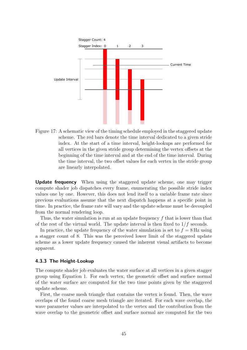
Update Interval

Stagger Index: 0 1 2 3

Stagger Count: 4

Current Time

Figure 17: A schematic view of the timing schedule employed in the staggered updatescheme. The red bars denote the time interval dedicated to a given strideindex. At the start of a time interval, height-lookups are performed forall vertices in the given stride group determining the vertex offsets at thebeginning of the time interval and at the end of the time interval. Duringthe time interval, the two offset values for each vertex in the stride groupare linearly interpolated.

Update frequency When using the staggered update scheme, one may triggercompute shader job dispatches every frame, enumerating the possible stride indexvalues one by one. However, this does not lend itself to a variable frame rate sinceprevious evaluations assume that the next dispatch happens at a specific point intime. In practice, the frame rate will vary and the update scheme must be decoupledfrom the normal rendering loop.

Thus, the water simulation is run at an update frequency f that is lower than thatof the rest of the virtual world. The update interval is then fixed to 1/f seconds.

In practice, the update frequency of the water simulation is set to f = 8 Hz usinga stagger count of 8. This was the perceived lower limit of the staggered updatescheme as a lower update frequency caused the inherent visual artifacts to becomeapparent.

4.3.3 The Height-Lookup

The compute shader job evaluates the water surface at all vertices in a given staggergroup using Equation 1. For each vertex, the geometric offset and surface normalof the water surface are computed for the two time points given by the staggeredupdate scheme.

First, the coarse mesh triangle that contains the vertex is found. Then, the waveoverlaps of the found coarse mesh triangle are iterated. For each wave overlap, thewave parameter values are interpolated to the vertex and the contribution from thewave overlap to the geometric offset and surface normal are computed for the two

45

time points using the wave profile. Finally, the contributions from all wave overlapsare accumulated and the final geometric offset and surface normal for the vertex iswritten to the vertex displacement buffer.

In order to avoid aliasing due to the Nyquist limit, each contribution is attenuatedaccording to the wavelength of the wave overlap. Since the wave overlaps are sortedby wavelength in descending order, the iteration terminates whenever the contribu-tion of a wave overlap is zero due to attenuation. This scheme improves performanceas it limits the compute shader execution time for coarse mesh triangles that are faraway from the camera.

Coarse mesh triangle lookup A top-down 2-dimensional grid implemented as anindex buffer is used to accelerate the lookup of coarse mesh triangles in the computeshader. The grid covers the water surface and each grid cell contains a referenceto the first element of a linked list of coarse mesh triangles intersecting that cell.All linked lists are packed into a single 2-value index buffer where the first valuereferences a coarse mesh triangle and the second value the next element in the linkedlist.

Thus, in order to find the coarse mesh triangle containing a 2-dimensional point ~pon the water surface, the grid cell i containing ~p is first found. Then, the grid indexbuffer is queried at i to get the index j referencing an element in the linked list indexbuffer. The linked list index buffer is subsequently queried at j for the coarse meshtriangle tj and the next index nj. If tj contains ~p in the plane, the procedure returnstj. Otherwise, the next element in the linked list is examined iteratively by settingj := nj. Finally, if an nj that does not point to another element is encountered,the end of the linked list has been reached and ~p must lie outside the bounds of thewater surface and the procedure returns nothing.

In practice, a constant grid size of 10242 was used. This results in a grid cell sidelength of approximately 4 m in a 16 km2 square-shaped simulation.

Wave filtering In order to eliminate aliasing on the water surface, the Nyquistlimit must be respected when waves are sampled. Thus, the contribution of a waveoverlap to the geometric offset is attenuated and filtered as described by Brunetonet al. [2010].

The sample size is the maximum world space distance between two vertices on thewater surface and the exact value can be determined from the leaf node scale in theposition buffer. However, if the exact value is used there will be visible discontinuitieson the water surface where leaf nodes at different depths in the quadtree are adjacent.In order to provide a seamless transition between leaf nodes, the approximate worldspace sample size, s, used when filtering is determined by

s =√

2 min(sx, sy),

where

46

sx =cx|~v|

|max(~vx/|~v|, ~vz/|~v|)|

sy =cy|~v||(~vy/|~v|)|

cx = 2 tan(fovx/2)rmin

w

cx = 2 tan(fovy/2)rmin

h

and ~v is the vector from the vertex to the camera in world space, fovx the horizontalfield of view, fovy the vertical field of view, w the screen width in pixels, h the screenheight in pixels and rmin the desired screen space extent of a triangle (in pixels) onthe water surface as described in Section 4.3.1.

The wavelength used when filtering is the minimum wavelength value stored onthe wave overlap as described in Section 4.2.9.

Wave parameter interpolation In order to evaluate the wave function (Equation1) at any point within a coarse mesh triangle, the wave parameter values stored ineach wave overlap are interpolated as shown by Jeschke and Wojtan [2015].

First, the barycentric coordinates, ~b, of a point ~p are computed with respect tothe corner points of the triangle as shown by Ericson [2004]. Then, when the waveoverlaps of the triangle are iterated, the three corner values of each wave parameterare linearly interpolated yielding a value for each wave parameter at ~p:

φ =(φ0 φ1 φ2

)T ·~ba =

(a0 a1 a2

)T ·~bc =

(c0 c1 c2

)T ·~b~d =

[~d0

~d1~d2

]~b

/∣∣∣[~d0~d1

~d2

]~b∣∣∣

where · denotes the dot product.Side-vertex interpolation [Jeschke and Wojtan, 2015] was also implemented but

not used due to the increased instruction count compared to linear interpolation.

Wave profile A trochoidal wave profile is used to offset the water surface in boththe vertical and horizontal directions as shown by Finch [2004] and Bruneton et al.[2010]. In contrast to their work, however, waves do not travel at constant phasespeeds and the phase function must be utilized. Given a world space point, (x y z)T ,on the water surface, the offset point according to the wave profile, ~p, is then:

~p =

xyz

+N∑i=1

dixai cos(ωiφi − ωit)

ai sin(ωiφi − ωit)

diyai cos(ωiφi − ωit)

,

47

where ωi the angular frequency of wave overlap i and ~di the interpolated direction,ai the interpolated amplitude and φi the interpolated phase of wave overlap i at(x y z)T . In order to calculate the surface normal at ~p, the partial derivatives of ~pis first calculated in the x and z directions, resulting in the surface tangent, ~t, andbitangent, ~b, respectively:

~t =∂

∂x~p

=

100

+N∑i=1

−dixai sin(ωiφi − ωit)

ai cos(ωiφi − ωit)

−diyai sin(ωiφi − ωit)

ωi∂

∂xφi

=

100

+N∑i=1

−dixai sin(ωiφi − ωit)

ai cos(ωiφi − ωit)

−diyai sin(ωiφi − ωit)

ωidixci

~b =∂

∂z~p

=

001

+N∑i=1

−dixai sin(ωiφi − ωit)

ai cos(ωiφi − ωit)

−diyai sin(ωiφi − ωit)

ωi∂

∂zφi

=

001

+N∑i=1

−dixai sin(ωiφi − ωit)

ai cos(ωiφi − ωit)

−diyai sin(ωiφi − ωit)

ωidiyci

,where ci is the interpolated phase speed of wave overlap i at (x y z)T .The surface normal, ~n, can then be calculated using the cross product:

~n =~b× ~t|~b× ~t|

.

48

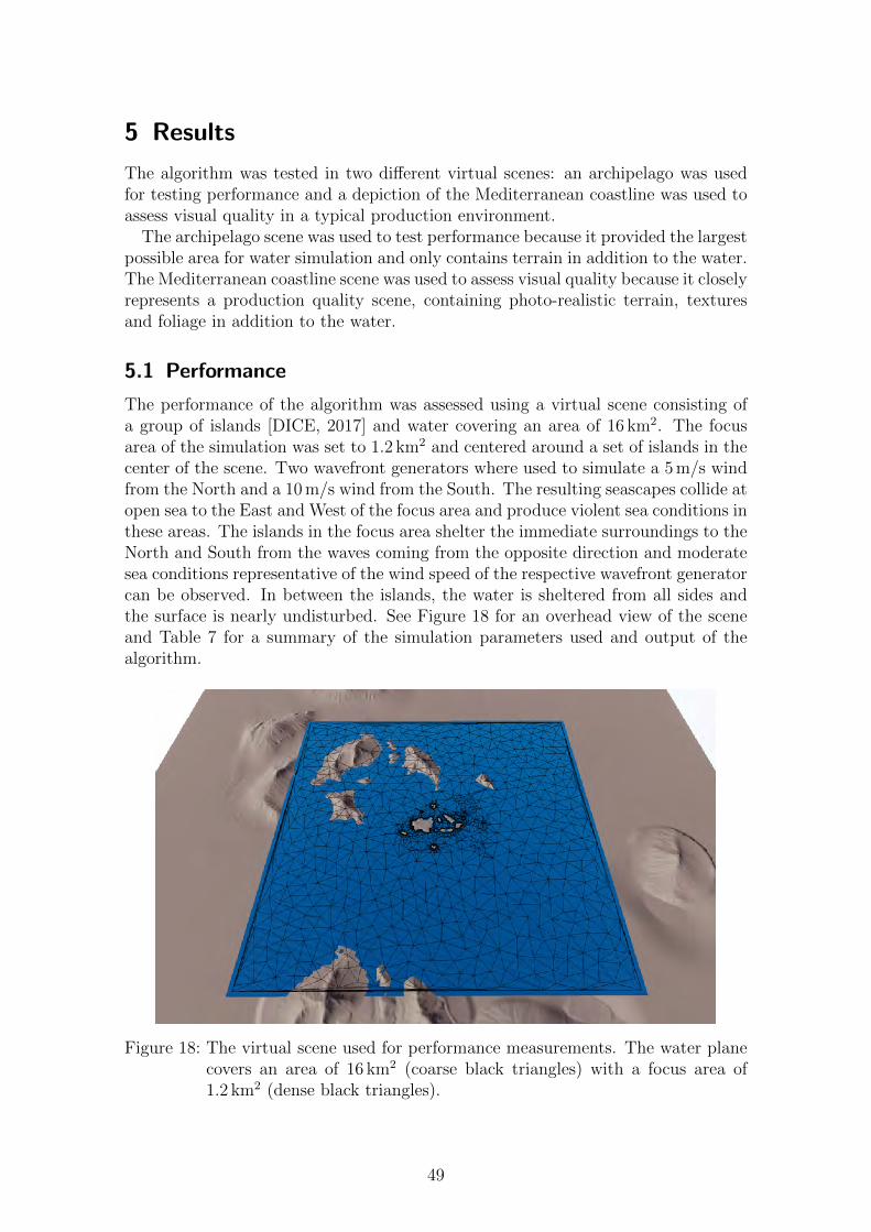
5 Results

The algorithm was tested in two different virtual scenes: an archipelago was usedfor testing performance and a depiction of the Mediterranean coastline was used toassess visual quality in a typical production environment.

The archipelago scene was used to test performance because it provided the largestpossible area for water simulation and only contains terrain in addition to the water.The Mediterranean coastline scene was used to assess visual quality because it closelyrepresents a production quality scene, containing photo-realistic terrain, texturesand foliage in addition to the water.

5.1 Performance

The performance of the algorithm was assessed using a virtual scene consisting ofa group of islands [DICE, 2017] and water covering an area of 16 km2. The focusarea of the simulation was set to 1.2 km2 and centered around a set of islands in thecenter of the scene. Two wavefront generators where used to simulate a 5 m/s windfrom the North and a 10 m/s wind from the South. The resulting seascapes collide atopen sea to the East and West of the focus area and produce violent sea conditions inthese areas. The islands in the focus area shelter the immediate surroundings to theNorth and South from the waves coming from the opposite direction and moderatesea conditions representative of the wind speed of the respective wavefront generatorcan be observed. In between the islands, the water is sheltered from all sides andthe surface is nearly undisturbed. See Figure 18 for an overhead view of the sceneand Table 7 for a summary of the simulation parameters used and output of thealgorithm.

Figure 18: The virtual scene used for performance measurements. The water planecovers an area of 16 km2 (coarse black triangles) with a focus area of1.2 km2 (dense black triangles).

49

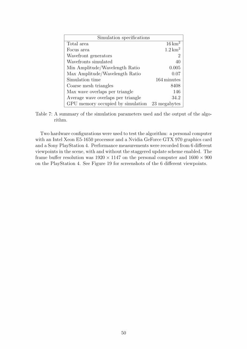
Simulation specificationsTotal area 16 km2

Focus area 1.2 km2

Wavefront generators 2Wavefronts simulated 40Min Amplitude/Wavelength Ratio 0.005Max Amplitude/Wavelength Ratio 0.07Simulation time 164 minutesCoarse mesh triangles 8408Max wave overlaps per triangle 146Average wave overlaps per triangle 34.2GPU memory occupied by simulation 23 megabytes

Table 7: A summary of the simulation parameters used and the output of the algo-rithm.

Two hardware configurations were used to test the algorithm: a personal computerwith an Intel Xeon E5-1650 processor and a Nvidia GeForce GTX 970 graphics cardand a Sony PlayStation 4. Performance measurements were recorded from 6 differentviewpoints in the scene, with and without the staggered update scheme enabled. Theframe buffer resolution was 1920 × 1147 on the personal computer and 1600 × 900on the PlayStation 4. See Figure 19 for screenshots of the 6 different viewpoints.

50

(a) Open sea South of island cluster (b) Southern inlet of island cluster

(c) Violent sea East of island cluster (d) Southern shoreline of South island

(e) Calm water in between islands (f) Northern shoreline of North island

Figure 19: Screenshots of the six viewpoints at which performance measurementswere recorded.

The total water surface evaluation time for a given viewpoint can be seen inTable 8. This corresponds to the total time consumed by the compute shader jobdispatches on the GPU. The coarse mesh triangle lookup time can be seen in Table9 and corresponds to the time it takes to find the coarse mesh triangle of interest forall vertices of a given stagger group in the vertex displacement buffer on the GPU,when using the staggered update scheme. Both of these measurements correspondto the part of the algorithm that must be executed independently of the number ofscreen pixels the water occupies in a rendered frame.

It is clear from these measurements that most time is typically spent accessing thewave data of the coarse mesh triangle as opposed to looking up the triangle itself.

51

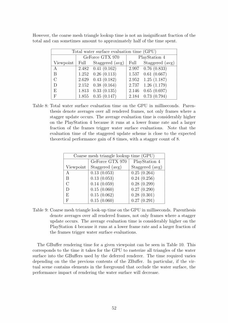
However, the coarse mesh triangle lookup time is not an insignificant fraction of thetotal and can sometimes amount to approximately half of the time spent.

Total water surface evaluation time (GPU)GeForce GTX 970 PlayStation 4

Viewpoint Full Staggered (avg) Full Staggered (avg)A 2.482 0.41 (0.162) 2.997 0.76 (0.833)B 1.252 0.26 (0.113) 1.537 0.61 (0.667)C 2.629 0.43 (0.182) 2.952 1.25 (1.187)D 2.152 0.38 (0.164) 2.737 1.26 (1.179)E 1.813 0.33 (0.135) 2.146 0.65 (0.697)F 1.855 0.35 (0.147) 2.184 0.73 (0.794)

Table 8: Total water surface evaluation time on the GPU in milliseconds. Paren-thesis denote averages over all rendered frames, not only frames where astagger update occurs. The average evaluation time is considerably higheron the PlayStation 4 because it runs at a lower frame rate and a largerfraction of the frames trigger water surface evaluations. Note that theevaluation time of the staggered update scheme is close to the expectedtheoretical performance gain of 8 times, with a stagger count of 8.

Coarse mesh triangle lookup time (GPU)GeForce GTX 970 PlayStation 4

Viewpoint Staggered (avg) Staggered (avg)A 0.13 (0.053) 0.25 (0.264)B 0.13 (0.053) 0.24 (0.256)C 0.14 (0.059) 0.28 (0.299)D 0.15 (0.060) 0.27 (0.290)E 0.15 (0.062) 0.28 (0.301)F 0.15 (0.060) 0.27 (0.291)

Table 9: Coarse mesh triangle look-up time on the GPU in milliseconds. Parenthesisdenote averages over all rendered frames, not only frames where a staggerupdate occurs. The average evaluation time is considerably higher on thePlayStation 4 because it runs at a lower frame rate and a larger fraction ofthe frames trigger water surface evaluations.

The GBuffer rendering time for a given viewpoint can be seen in Table 10. Thiscorresponds to the time it takes for the GPU to rasterize all triangles of the watersurface into the GBuffers used by the deferred renderer. The time required variesdepending on the the previous contents of the ZBuffer. In particular, if the vir-tual scene contains elements in the foreground that occlude the water surface, theperformance impact of rendering the water surface will decrease.

52

GBuffer rendering time (GPU)Viewpoint GeForce GTX 970 PlayStation 4A 2.103 3.749B 1.895 2.774C 2.111 3.474D 2.046 3.409E 1.926 3.615F 1.777 2.497

Table 10: GBuffer rendering time on the GPU in milliseconds

The Quadtree & buffer construction time for a given viewpoint can be seen inTable 11. This corresponds to the time it takes to build the quadtree and fill thecontents of the dynamic render buffers every frame for one core of the CPU. The jobis scheduled to be executed alongside other independent jobs in order to maximizeprocessor utilization when multiple cores are available.

Quadtree & render buffer construction time (CPU)Viewpoint Intel Xeon E5-1650 PlayStation 4A 1.941 3.434B 1.522 2.558C 1.883 3.115D 1.927 3.348E 1.923 3.413F 1.869 3.160

Table 11: Quadtree & render buffer construction time on the CPU in milliseconds

5.2 Achieved Visual Quality

The visual quality of frames generated by the algorithm was assessed using a virtualscene depicting the Mediterranean coast [DICE, 2017]. One wavefront generatorwas used and the wind direction was set to face the coastline.

5.2.1 Overview

See Figure 20 for screenshots of six viewpoints representative of the visual qualitythat can be achieved when using the algorithm in a typical production environment.In order to see the wave patterns produced on a grand scale, Figure 21 shows aseries of screenshots from a top-down perspective as the altitude increases.

53

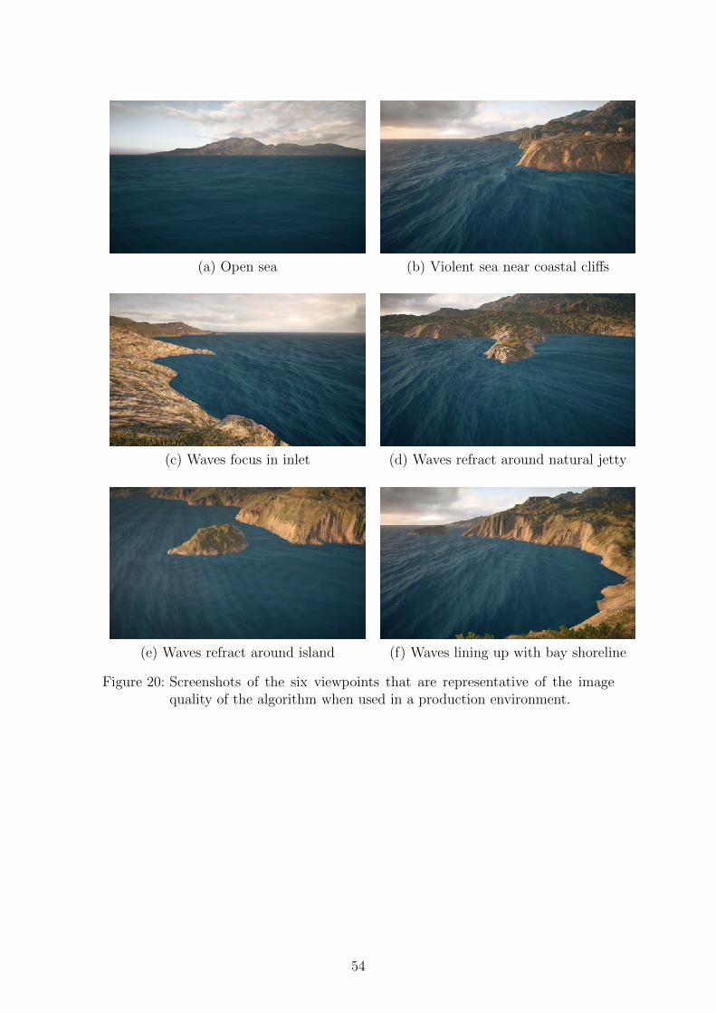
(a) Open sea (b) Violent sea near coastal cliffs

(c) Waves focus in inlet (d) Waves refract around natural jetty

(e) Waves refract around island (f) Waves lining up with bay shoreline

Figure 20: Screenshots of the six viewpoints that are representative of the imagequality of the algorithm when used in a production environment.

54

Figure 21: Screenshots from a top-down view as the altitude increases

In practice, there is no visible aliasing. The employed wave filtering effectivelyeliminates spatial aliasing and even though a low update frequency is used for thestaggered update scheme, no temporal aliasing was observed.

55

Repetition patterns can be observed in areas close to the boundaries of the sim-ulation where wavefronts have not yet started to diverge due to changes in depth.However, note that as each coarse mesh triangle can be visually unique, it is pos-sible to eliminate repetition patterns in theory even close to the boundaries of thesimulation.

In theory, cracks in the water surface geometry are expected in places where leafnodes at different depths in the world space quadtree are adjacent since staggergroup indices only line up at the borders of adjacent leaf nodes that have the sameworld space size. In practice, no visible cracks in the water surface can be observed.

Visible seams between coarse mesh triangles can be observed if a high frequencywave is visible in one triangle but gets filtered in an adjacent triangle due to in-adequate sampling resolution. The reason for this behavior is that the minimumwavelength value of the three corners of a wave overlap is used when filtering wavesas described in Section 4.3.3 and the wave is not attenuated within the coarse meshtriangle in which it is visible.

5.2.2 Captured Water Wave Behaviors

The following section illustrates specific wave behaviors that are captured by thesimulation.

Refraction A water wave refracts as it moves from one depth to another and pointson the wave travel at different phase speeds. Within the simulation, a wavefrontrefracts if the change in the underlying depth field is significant. See Figure 22 for aview of a single wavefront developing a swallowtail pattern as it enters a local areaof shallow water.

(a) Simulation step (b) Rendering step

Figure 22: A wavefront refracts to produce a swallowtail pattern as it enters a localshallow area of the seafloor. a) Multiple time steps of the wavefront areshown transitioning from green to red with increasing phase. The coarsetriangle mesh is shown in black. The seafloor is shown in gray. b) Therendered water surface.

Reflection A water wave reflects when it collides with hard surfaces. Within thesimulation, a wavefront reflects when it intersects scene geometry. See Figure 23 fora view of a single wavefront as it reflects off the shoreline.

56

(a) Simulation step (b) Rendering step

Figure 23: A wavefront reflecting off the shoreline within the simulation. a) Multipletime steps of the wavefront are shown transitioning from green to redwith increasing phase. The coarse triangle mesh is shown in black. Theseafloor is shown in gray. b) The rendered water surface. Note the nulllines that appear where reflected waves cancel each other out.

Dispersion Water waves of different wavenumbers travel at different phase speedsdue to dispersion. Within the simulation, this phenomenon is handled naturallyby the integration scheme used. See Figure 24 for a view of multiple wavefrontstravelling at different phase speeds.

(a) Simulation step (b) Rendering step

Figure 24: Dispersion within the simulation. a) The coarse triangle mesh is shownin black. Due to the amount of information, wavefront time steps are notshown. b) The rendered water surface.

57

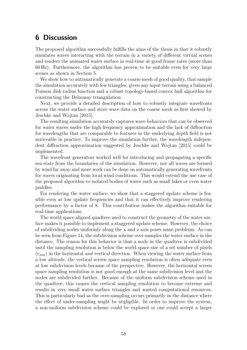
6 Discussion

The proposed algorithm successfully fulfills the aims of the thesis in that it robustlysimulates waves interacting with the terrain in a variety of different virtual scenesand renders the animated water surface in real-time at good frame rates (more than60 Hz). Furthermore, the algorithm has proven to be suitable even for very largescenes as shown in Section 5.

We show how to automatically generate a coarse mesh of good quality, that samplethe simulation accurately with few triangles, given any input terrain using a balancedPoisson disk radius function and a robust topology-based convex hull algorithm forconstructing the Delaunay triangulation.

Next, we provide a detailed description of how to robustly integrate wavefrontsacross the water surface and store wave data on the coarse mesh as first showed byJeschke and Wojtan [2015].

The resulting simulation accurately captures wave behaviors that can be observedfor water waves under the high frequency approximation and the lack of diffractionfor wavelengths that are comparable to features in the underlying depth field is notnoticeable in practice. To improve the simulation further, the wavelength indepen-dent diffraction approximation suggested by Jeschke and Wojtan [2015] could beimplemented.

The wavefront generators worked well for introducing and propagating a specificsea state from the boundaries of the simulation. However, not all waves are formedby wind far away and more work can be done on automatically generating wavefrontsfor waves originating from local wind conditions. This would extend the use case ofthe proposed algorithm to isolated bodies of water such as small lakes or even waterpuddles.

For rendering the water surface, we show that a staggered update scheme is fea-sible even at low update frequencies and that it can effectively improve renderingperformance by a factor of 8. This contribution makes the algorithm suitable forreal-time applications.

The world space aligned quadtree used to construct the geometry of the water sur-face makes it possible to implement a staggered update scheme. However, the choiceof subdividing nodes uniformly along the x and z axis poses some problems. As canbe seen from Figure 14, the subdivision scheme over-samples the water surface in thedistance. The reason for this behavior is that a node in the quadtree is subdivideduntil the sampling resolution is below the world space size of a set number of pixels(rmin) in the horizontal and vertical direction. When viewing the water surface froma low altitude, the vertical screen space sampling resolution is often adequate evenat low subdivision levels because of the perspective. However, the horizontal screenspace sampling resolution is not good enough at the same subdivision level and thenodes are subdivided further. Because of the uniform subdivision scheme used inthe quadtree, this causes the vertical sampling resolution to become extreme andresults in very small water surface triangles and wasted computational resources.This is particularly bad as the over-sampling occurs primarily in the distance wherethe effect of under-sampling might be negligible. In order to improve the system,a non-uniform subdivision scheme could be explored or one could accept a larger

58

screen space sampling resolution in the horizontal direction and stop subdivisiononce adequate resolution is reached in any direction.

For performing height-lookups on the water surface, linear interpolation of waveparameters proved to be sufficient. The difference between linear and side-vertexinterpolation was not apparent in our test cases because there were often multipletriangles, piecewise approximating wavefront curvature, in areas where wavefrontstend to refract as a result of the tessellation scheme employed to construct thecoarse mesh. Thus, the negligible improvement in visual quality provided by thehigher order interpolation scheme did not outweigh the increased instruction countrequired.

To completely avoid visible seams between coarse mesh triangles, one should ide-ally interpolate the wavelength at each corner of a wave overlap and attenuate wavesaccording to this value when filtering wave overlaps, as opposed to the minimum ofthe three values. The stopping criterion can use the minimum value for performanceconsiderations, but the attenuation should work with the interpolated value in orderto avoid discontinuities in which waves appear on adjacent coarse mesh triangles.

6.1 Cache Coherence

Vertex displacement buffer The persistent vertex displacement buffer is sparseby construction. As slots are allocated and deallocated the buffer will become frag-mented with respect to the world space locations of the leaf nodes it references.The displacement stored for vertices within a leaf node will be close in memory butslots of leaf nodes that are adjacent in world space might be far apart in the vertexdisplacement buffer, or even belong to different render buffer groups entirely.

Ideally, to use the shared memory on the GPU effectively, one would like theslots of leaf nodes that cover a particular coarse mesh triangle to be in the samevertex displacement buffer and to be close in memory within the buffer itself. Then,compute shader threads executing in the same warp and thread group will accessthe same wave data and use the shared memory of the thread group more effec-tively. This is the case if the slots of adjacent leaf nodes are adjacent in the vertexdisplacement buffer.

To solve the issue, the vertex displacement buffer should be defragmented in someway. An idea for a defragmentation routine is to switch the slots of two leaf nodesin the buffer every frame so that slots become gradually sorted by the distance tothe viewer.

Static coarse mesh The proposed algorithm as outlined is this thesis and byJeschke and Wojtan [2015] considers a static coarse mesh independent of the viewfrustum chosen at runtime. Even though the coarse mesh is adaptively tessellated tohandle scale differences, too small coarse mesh triangles are not feasible in practicebecause they cause memory access coherency issues when viewed from afar.

For example, consider a long stretch of rugged coastline where the coarse mesh isfinely tessellated. The evaluation of two neighboring vertices on the water surface(that are executed in the same warp or thread group in the compute shader) mightaccess widely different wave data if the vertices happen to be located in two different

59

coarse mesh triangles. When the rugged coastline is viewed from a distance, a smallscreen space area may contain a large number of different coarse mesh triangles andcause an enormous amount of cache misses. Since accessing wave data is typicallythe most performance intensive task of evaluating the water surface (See Section5.1), incoherent memory accesses can be particularly bad for the performance of thealgorithm.

Note that this is not a problem for small triangles that are close to the viewersince they occupy a large amount of screen space and thus a large number of verticeson the water surface geometry.

See Section 7.2 for a potential solution to this problem.

60

7 Future Work

7.1 Coarse Mesh As Water Surface Geometry

The coarse mesh tree could potentially be used for rendering, eliminating the needfor the coarse mesh triangle lookup procedure when evaluating the water surface.As the lookup time can amount to approximately 50% of the total evaluation time insome cases (See Section 5.1), this would result in increased rendering performance.

Since the coarse mesh is spatially coarse by definition, it would have to be tessel-lated in a view-dependent manner to be used to directly represent the water surface.This could be done similarly to how the world space quadtree is tessellated in Sec-tion 4.3.1. Then, any vertex on the water surface would simply need to traverse thesubdivision tree upwards to find the set of wave overlaps to iterate.

7.2 Coarse Mesh Tree

To solve the cache coherence problem described in Section 6.1, we propose recordingwave parameters in a coarse mesh tree where the tessellation factor can be chosen atruntime so that each coarse mesh triangle occupies approximately the same screenspace area. Since wave parameters will need to be stored separately for each sub-division level of a coarse mesh triangle, the approach will be limited by its memoryfootprint.

In order to construct the coarse mesh tree, the triangles of a coarse mesh may besubdivided until they reach a desired detail level. The simulation can then recordwave parameters onto the highest level of detail (LOD) representation in the coarsemesh tree. Once wavefront propagation and recording is done, finished chains canbe propagated to a lower LOD in the tree by replacing two chains from two coarsemesh edges that share a sample in the high LOD representation with a single chainon the single coarse mesh edge in the lower LOD representation. See Figure 25 fora graphical explanation of the proposed procedure.

61

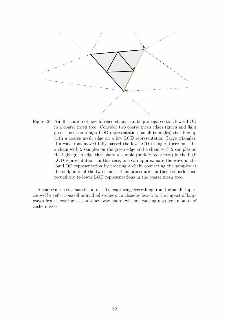
Figure 25: An illustration of how finished chains can be propagated to a lower LODin a coarse mesh tree. Consider two coarse mesh edges (green and lightgreen lines) on a high LOD representation (small triangles) that line upwith a coarse mesh edge on a low LOD representation (large triangle).If a wavefront moved fully passed the low LOD triangle, there must bea chain with 2 samples on the green edge and a chain with 2 samples onthe light green edge that share a sample (middle red arrow) in the highLOD representation. In this case, one can approximate the wave in thelow LOD representation by creating a chain connecting the samples atthe endpoints of the two chains. This procedure can then be performedrecursively to lower LOD representations in the coarse mesh tree.

A coarse mesh tree has the potential of capturing everything from the small ripplescaused by reflections off individual stones on a close-by beach to the impact of largewaves from a roaring sea on a far away shore, without causing massive amounts ofcache misses.

62

8 Conclusion

An algorithm for rendering large expanses of water that interact with the terrainof the virtual scene in real-time was presented. The simulation robustly propagatesand records wavefronts across the water surface in a pre-computation step whiletaking the shape of the terrain into account. As a result, the refraction, reflectionand dispersion phenomena of the water waves are captured and the simulation canaccurately represent both deep water waves and shallow water waves. During run-time, the simulation is evaluated using a staggered update scheme and the watersurface is rendered using an adaptively tessellated world space aligned quadtree.

The staggered update scheme utilizes the observation that the water simulationcan be evaluated at a low update frequency without loss of visual quality and effec-tively improves the performance by a factor of 8 as the computational workload issplit across multiple frames.

In future work, a coarse mesh tree could be explored in order to improve cachecoherence, which is the perceived bottleneck of the algorithm, and eliminate a lookupprocedure to further improve rendering performance.

9 Acknowledgements

I would like to thank my advisors Fredrik Larsson and Jan Schmid (DICE), my co-worker Andreas Wennstrom and my academic supervisor Erik Sintorn (Chalmers)for helping me realize the thesis. In particular, I would like to thank my advisors atDICE for coming up with the idea of the staggered update scheme.

63

References

George Biddell Airy. Tides and waves. Encyclopaedia Metropolitana, pages 241–396,1841.

Franz Aurenhammer. Voronoi Diagrams—a Survey of a Fundamental GeometricData Structure. ACM Comput. Surv., 23(3):345–405, September 1991. ISSN0360-0300. doi: 10.1145/116873.116880. URL http://doi.acm.org/10.1145/

116873.116880.

C. Bradford Barber, David P. Dobkin, and Hannu Huhdanpaa. The QuickhullAlgorithm for Convex Hulls. ACM Trans. Math. Softw., 22(4):469–483, December1996. ISSN 0098-3500. doi: 10.1145/235815.235821. URL http://doi.acm.org/

10.1145/235815.235821.

Robert Bridson. Fast Poisson Disk Sampling in Arbitrary Dimensions. In ACMSIGGRAPH 2007 Sketches, SIGGRAPH ’07, New York, NY, USA, 2007. ACM.ISBN 978-1-4503-4726-6. doi: 10.1145/1278780.1278807. URL http://doi.acm.

org/10.1145/1278780.1278807.

Kevin Q. Brown. Voronoi diagrams from convex hulls. Information Pro-cessing Letters, 9(5):223–228, December 1979. ISSN 0020-0190. doi: 10.1016/0020-0190(79)90074-7. URL http://www.sciencedirect.com/science/

article/pii/0020019079900747.

Eric Bruneton, Fabrice Neyret, and Nicolas Holzschuch. Real-time Realistic OceanLighting using Seamless Transitions from Geometry to BRDF. Computer GraphicsForum, 29(2):487–496, May 2010. ISSN 1467-8659. doi: 10.1111/j.1467-8659.2009.01618.x. URL http://onlinelibrary.wiley.com/doi/10.1111/j.1467-8659.

2009.01618.x/abstract.

Robert L. Cook. Stochastic Sampling in Computer Graphics. ACM Trans. Graph.,5(1):51–72, January 1986. ISSN 0730-0301. doi: 10.1145/7529.8927. URL http:

//doi.acm.org/10.1145/7529.8927.

DICE. DICE, 2017. URL http://www.dice.se/.

H. Edelsbrunner and N. R. Shah. Incremental Topological Flipping Works forRegular Triangulations. In Proceedings of the Eighth Annual Symposium onComputational Geometry, SCG ’92, pages 43–52, New York, NY, USA, 1992.ACM. ISBN 978-0-89791-517-5. doi: 10.1145/142675.142688. URL http:

//doi.acm.org/10.1145/142675.142688.

Herbert Edelsbrunner and Raimund Seidel. Voronoi Diagrams and Arrangements.In Proceedings of the First Annual Symposium on Computational Geometry, SCG’85, pages 251–262, New York, NY, USA, 1985. ACM. ISBN 978-0-89791-163-4. doi: 10.1145/323233.323266. URL http://doi.acm.org/10.1145/323233.

323266.

64

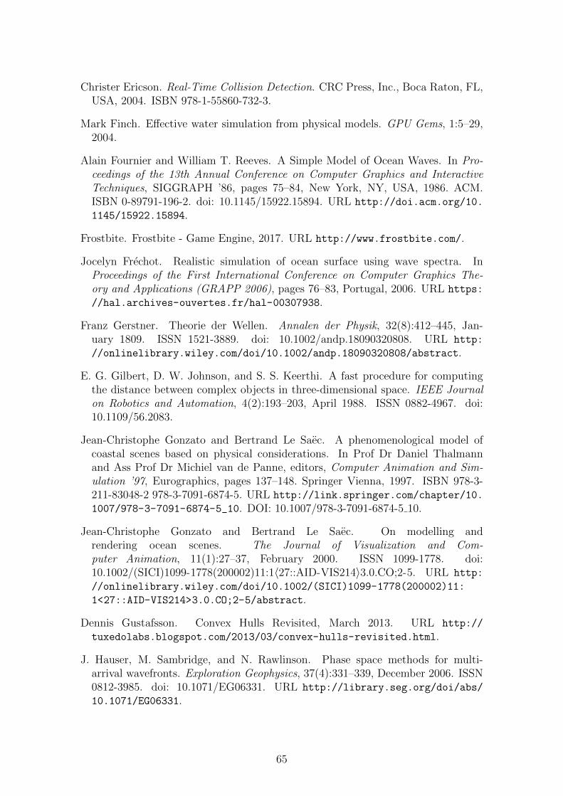
Christer Ericson. Real-Time Collision Detection. CRC Press, Inc., Boca Raton, FL,USA, 2004. ISBN 978-1-55860-732-3.

Mark Finch. Effective water simulation from physical models. GPU Gems, 1:5–29,2004.

Alain Fournier and William T. Reeves. A Simple Model of Ocean Waves. In Pro-ceedings of the 13th Annual Conference on Computer Graphics and InteractiveTechniques, SIGGRAPH ’86, pages 75–84, New York, NY, USA, 1986. ACM.ISBN 0-89791-196-2. doi: 10.1145/15922.15894. URL http://doi.acm.org/10.

1145/15922.15894.

Frostbite. Frostbite - Game Engine, 2017. URL http://www.frostbite.com/.

Jocelyn Frechot. Realistic simulation of ocean surface using wave spectra. InProceedings of the First International Conference on Computer Graphics The-ory and Applications (GRAPP 2006), pages 76–83, Portugal, 2006. URL https:

//hal.archives-ouvertes.fr/hal-00307938.

Franz Gerstner. Theorie der Wellen. Annalen der Physik, 32(8):412–445, Jan-uary 1809. ISSN 1521-3889. doi: 10.1002/andp.18090320808. URL http:

//onlinelibrary.wiley.com/doi/10.1002/andp.18090320808/abstract.

E. G. Gilbert, D. W. Johnson, and S. S. Keerthi. A fast procedure for computingthe distance between complex objects in three-dimensional space. IEEE Journalon Robotics and Automation, 4(2):193–203, April 1988. ISSN 0882-4967. doi:10.1109/56.2083.

Jean-Christophe Gonzato and Bertrand Le Saec. A phenomenological model ofcoastal scenes based on physical considerations. In Prof Dr Daniel Thalmannand Ass Prof Dr Michiel van de Panne, editors, Computer Animation and Sim-ulation ’97, Eurographics, pages 137–148. Springer Vienna, 1997. ISBN 978-3-211-83048-2 978-3-7091-6874-5. URL http://link.springer.com/chapter/10.

1007/978-3-7091-6874-5_10. DOI: 10.1007/978-3-7091-6874-5 10.

Jean-Christophe Gonzato and Bertrand Le Saec. On modelling andrendering ocean scenes. The Journal of Visualization and Com-puter Animation, 11(1):27–37, February 2000. ISSN 1099-1778. doi:10.1002/(SICI)1099-1778(200002)11:1〈27::AID-VIS214〉3.0.CO;2-5. URL http:

//onlinelibrary.wiley.com/doi/10.1002/(SICI)1099-1778(200002)11:

1<27::AID-VIS214>3.0.CO;2-5/abstract.

Dennis Gustafsson. Convex Hulls Revisited, March 2013. URL http://

tuxedolabs.blogspot.com/2013/03/convex-hulls-revisited.html.

J. Hauser, M. Sambridge, and N. Rawlinson. Phase space methods for multi-arrival wavefronts. Exploration Geophysics, 37(4):331–339, December 2006. ISSN0812-3985. doi: 10.1071/EG06331. URL http://library.seg.org/doi/abs/

10.1071/EG06331.

65

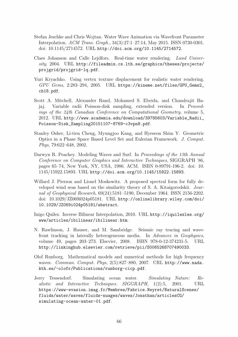
Stefan Jeschke and Chris Wojtan. Water Wave Animation via Wavefront ParameterInterpolation. ACM Trans. Graph., 34(3):27:1–27:14, May 2015. ISSN 0730-0301.doi: 10.1145/2714572. URL http://doi.acm.org/10.1145/2714572.

Claes Johanson and Calle Lejdfors. Real-time water rendering. Lund Univer-sity, 2004. URL http://fileadmin.cs.lth.se/graphics/theses/projects/

projgrid/projgrid-lq.pdf.

Yuri Kryachko. Using vertex texture displacement for realistic water rendering.GPU Gems, 2:283–294, 2005. URL https://kineme.net/files/GPU_Gems2_

ch18.pdf.

Scott A. Mitchell, Alexander Rand, Mohamed S. Ebeida, and Chandrajit Ba-jaj. Variable radii Poisson-disk sampling, extended version. In Proceed-ings of the 24th Canadian Conference on Computational Geometry, volume 5,2012. URL http://www.academia.edu/download/39785603/Variable_Radii_

Poisson-Disk_Sampling20151107-8769-c3vpn8.pdf.

Stanley Osher, Li-tien Cheng, Myungjoo Kang, and Hyeseon Shim Y. GeometricOptics in a Phase Space Based Level Set and Eulerian Framework. J. Comput.Phys, 79:622–648, 2002.

Darwyn R. Peachey. Modeling Waves and Surf. In Proceedings of the 13th AnnualConference on Computer Graphics and Interactive Techniques, SIGGRAPH ’86,pages 65–74, New York, NY, USA, 1986. ACM. ISBN 0-89791-196-2. doi: 10.1145/15922.15893. URL http://doi.acm.org/10.1145/15922.15893.

Willard J. Pierson and Lionel Moskowitz. A proposed spectral form for fully de-veloped wind seas based on the similarity theory of S. A. Kitaigorodskii. Jour-nal of Geophysical Research, 69(24):5181–5190, December 1964. ISSN 2156-2202.doi: 10.1029/JZ069i024p05181. URL http://onlinelibrary.wiley.com/doi/

10.1029/JZ069i024p05181/abstract.

Inigo Quilez. Inverse Bilinear Interpolation, 2010. URL http://iquilezles.org/

www/articles/ibilinear/ibilinear.htm.

N. Rawlinson, J. Hauser, and M. Sambridge. Seismic ray tracing and wave-front tracking in laterally heterogeneous media. In Advances in Geophysics,volume 49, pages 203–273. Elsevier, 2008. ISBN 978-0-12-374231-5. URLhttp://linkinghub.elsevier.com/retrieve/pii/S0065268707490033.

Olof Runborg. Mathematical models and numerical methods for high frequencywaves. Commun. Comput. Phys, 2(5):827–880, 2007. URL http://www.nada.

kth.se/~olofr/Publications/runborg-cicp.pdf.

Jerry Tessendorf. Simulating ocean water. Simulating Nature: Re-alistic and Interactive Techniques. SIGGRAPH, 1(2):5, 2001. URLhttps://www-evasion.imag.fr/Membres/Fabrice.Neyret/NaturalScenes/

fluids/water/waves/fluids-nuages/waves/Jonathan/articlesCG/

simulating-ocean-water-01.pdf.

66

Pauline Y. Ts’o and Brian A. Barsky. Modeling and Rendering Waves: Wave-tracingUsing Beta-splines and Reflective and Refractive Texture Mapping. ACM Trans.Graph., 6(3):191–214, July 1987. ISSN 0730-0301. doi: 10.1145/35068.35070.URL http://doi.acm.org/10.1145/35068.35070.

V. Vinje, E. Iversen, and H. Gjøystdal. Traveltime and amplitude estimation usingwavefront construction. GEOPHYSICS, 58(8):1157–1166, August 1993. ISSN0016-8033. doi: 10.1190/1.1443499. URL http://library.seg.org/doi/abs/

10.1190/1.1443499.

67