CALIFORNIA STATE UNIVERSITY, NORTHRIDGE

A HARDWARE IMPLEMENTATION OF

AN ARTIFICIAL NEURAL NETWORK

A graduate project submitted in partial fulfillment of the requirements

For the degree of Master of Science in Electrical Engineering

By

Justin Thomas Wodarck

December 2009

ii

The graduate project of Justin Thomas Wodarck is approved:

Nagwa Bekir, Ph.D. Date

Xiyi Hang, Ph.D. Date

Deborah van Alphen, Ph.D., Chair Date

California State University, Northridge

iii

DEDICATION

I would like to dedicate this report to my mom. I have only been able to accomplish what

I have thanks to her inspiration and sacrifice. She always said “people don’t care how

much you know, until they know how much you care.” She lived that out each and every

day of her life.

Roxanne Wodarck (1954 – 2007)

iv

ACKNOWLEDGEMENT

I would like to thank the LORD Jesus, my King and Savior, to whom I owe every neuron

in my brain and every ounce of my being. He has motivated me to always strive for

excellence and use my talents for love. One of the verses that has helped me during my

studies at CSUN:

“The fear of the LORD is the beginning of wisdom;

all who follow His precepts have good understanding.

To Him belongs eternal praise.” –Psalm 111:10 (NIV)

I would like to thank my Dad, whose constant tinkering, obsessive organization, and

ingenuity gave me the mind and attitude of a true engineer.

Special thanks to Dr. Deborah van Alphen, for mentoring me during this project.

And most importantly, I would like to thank my beautiful wife Jen, the best wife a guy

could ask for and the wonderful mother to our children: Gavin and Makayla. You guys

make me excited to come home at the end of every workday. You make life fun!

v

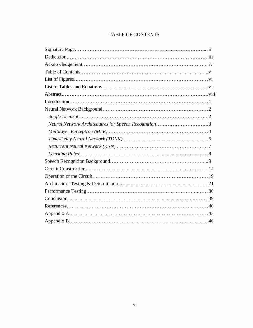
TABLE OF CONTENTS

Signature Page……………………………………………………………………... ii

Dedication…………………………………………………………………………. iii

Acknowledgement………………………………………………………………… iv

Table of Contents…………………………………………………………………... v

List of Figures……………………………………………………………………… vi

List of Tables and Equations ……………………………………………………….vii

Abstract…………………………………………………………………………….. viii

Introduction………………………………………………………………………… 1

Neural Network Background………………………………………………………. 2

Single Element…………………………………………………………………… 2

Neural Network Architectures for Speech Recognition………………………….. 3

Multilayer Perceptron (MLP) …………………………………………………… 4

Time-Delay Neural Network (TDNN) …………………………………………… 5

Recurrent Neural Network (RNN) ………………………………………………. 7

Learning Rules…………………………………………………………………… 8

Speech Recognition Background…………………………………………………... 9

Circuit Construction……………………………………………………………….. 14

Operation of the Circuit……………………………………………………………. 19

Architecture Testing & Determination…………………………………………….. 21

Performance Testing…………………………………………………………..…… 30

Conclusion…………………………………………………………………..……... 39

References…………………………………………………………………..……… 40

Appendix A………………………………………………………………………… 42

Appendix B………………………………………………………………………… 46

vi

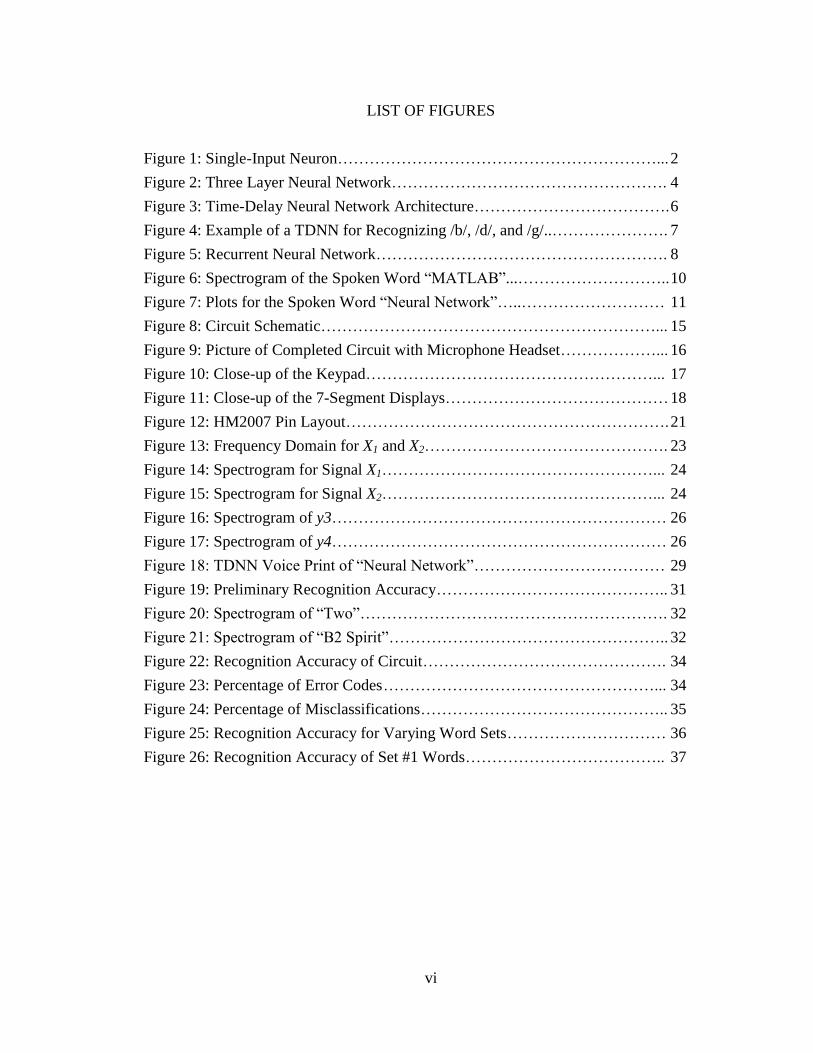
LIST OF FIGURES

Figure 1: Single-Input Neuron……………………………………………………... 2

Figure 2: Three Layer Neural Network……………………………………………. 4

Figure 3: Time-Delay Neural Network Architecture………………………………. 6

Figure 4: Example of a TDNN for Recognizing /b/, /d/, and /g/..…………………. 7

Figure 5: Recurrent Neural Network………………………………………………. 8

Figure 6: Spectrogram of the Spoken Word “MATLAB”...……………………….. 10

Figure 7: Plots for the Spoken Word “Neural Network”…..……………………… 11

Figure 8: Circuit Schematic………………………………………………………... 15

Figure 9: Picture of Completed Circuit with Microphone Headset………………... 16

Figure 10: Close-up of the Keypad………………………………………………... 17

Figure 11: Close-up of the 7-Segment Displays…………………………………… 18

Figure 12: HM2007 Pin Layout……………………………………………………. 21

Figure 13: Frequency Domain for X1 and X2………………………………………. 23

Figure 14: Spectrogram for Signal X1……………………………………………... 24

Figure 15: Spectrogram for Signal X2……………………………………………... 24

Figure 16: Spectrogram of y3……………………………………………………… 26

Figure 17: Spectrogram of y4……………………………………………………… 26

Figure 18: TDNN Voice Print of “Neural Network”……………………………… 29

Figure 19: Preliminary Recognition Accuracy…………………………………….. 31

Figure 20: Spectrogram of “Two”…………………………………………………. 32

Figure 21: Spectrogram of “B2 Spirit”…………………………………………….. 32

Figure 22: Recognition Accuracy of Circuit………………………………………. 34

Figure 23: Percentage of Error Codes ……………………………………………... 34

Figure 24: Percentage of Misclassifications……………………………………….. 35

Figure 25: Recognition Accuracy for Varying Word Sets………………………… 36

Figure 26: Recognition Accuracy of Set #1 Words……………………………….. 37

vii

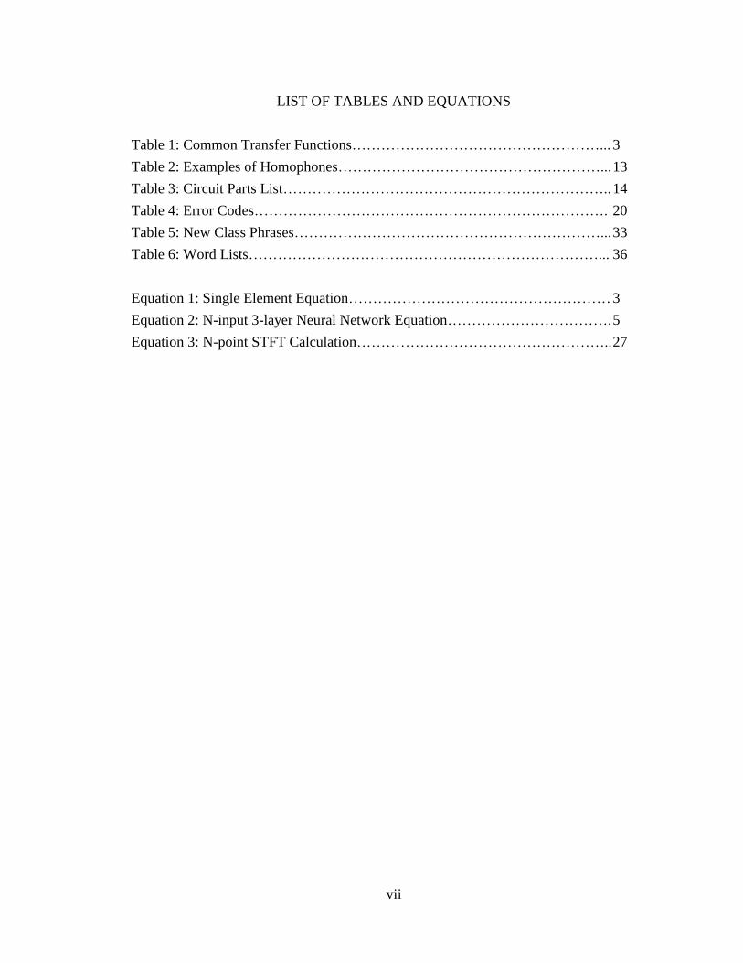
LIST OF TABLES AND EQUATIONS

Table 1: Common Transfer Functions……………………………………………... 3

Table 2: Examples of Homophones………………………………………………... 13

Table 3: Circuit Parts List………………………………………………………….. 14

Table 4: Error Codes………………………………………………………………. 20

Table 5: New Class Phrases………………………………………………………... 33

Table 6: Word Lists………………………………………………………………... 36

Equation 1: Single Element Equation……………………………………………… 3

Equation 2: N-input 3-layer Neural Network Equation……………………………. 5

Equation 3: N-point STFT Calculation…………………………………………….. 27

viii

ABSTRACT

A HARDWARE IMPLEMENTATION OF

AN ARTIFICIAL NEURAL NETWORK

By

Justin Thomas Wodarck

Master of Science in Electrical Engineering

This graduate project explores speech recognition utilizing an artificial neural network

circuit. A stand-alone hardware implementation of an unknown architecture neural

network was constructed around the HM2007 Integrated Circuit (IC) manufactured by

Hualon Microelectronics Corporation. A series of tests were conducted utilizing custom

coding in MATLAB to reverse-engineer the architecture of the IC and measure its

parameters. The performance of the completed circuit was tested for recognition accuracy

while changing variables such as total number of classes and word choice. A comparison

of performance between multisyllabic words and homophones was also conducted.

1

Introduction

Many people believe that neural network research and applications died with the

published work of Minsky and Papert in 1969 [1]. Their research showed that despite all

the initial hype surrounding neural networks, this new mathematical model couldn’t even

solve the basic exclusive-or (XOR) logic gate. What fewer people know is that with the

addition of multiple layers and more complex architectures these limitation in neural

networks could not only be overcome, but they could flourish in a variety of applications.

Recently, neural networks have found success in a diverse range of uses over numerous

fields including: stock market analysis, high performance aircraft autopilots, weapons

target tracking, telecommunication image and data compression, and speech recognition

to name a few [2]. The goal of this Graduate Project was to explore speech recognition

with neural networks. The objectives were to: construct a stand-alone hardware

implementation of an artificial neural network around the HM2007 Integrated Circuit

(IC), determine the architecture and learning style used by this IC via experimentation,

and test the completed circuit to characterize performance.

2

Neural Network Background

Neural networks are based on the classification ability and learning processes of the

human brain. By starting with simple elements and highly interconnecting them, neural

networks are able to perform extremely complex pattern classification and function

approximation. This section describes the starting point for understanding of neural

networks and the architectures investigated in this project. A more exhaustive

background can be found in Neural Network Design [3], and Handbook of Neural

Networks for Speech Processing [4].

Single Element

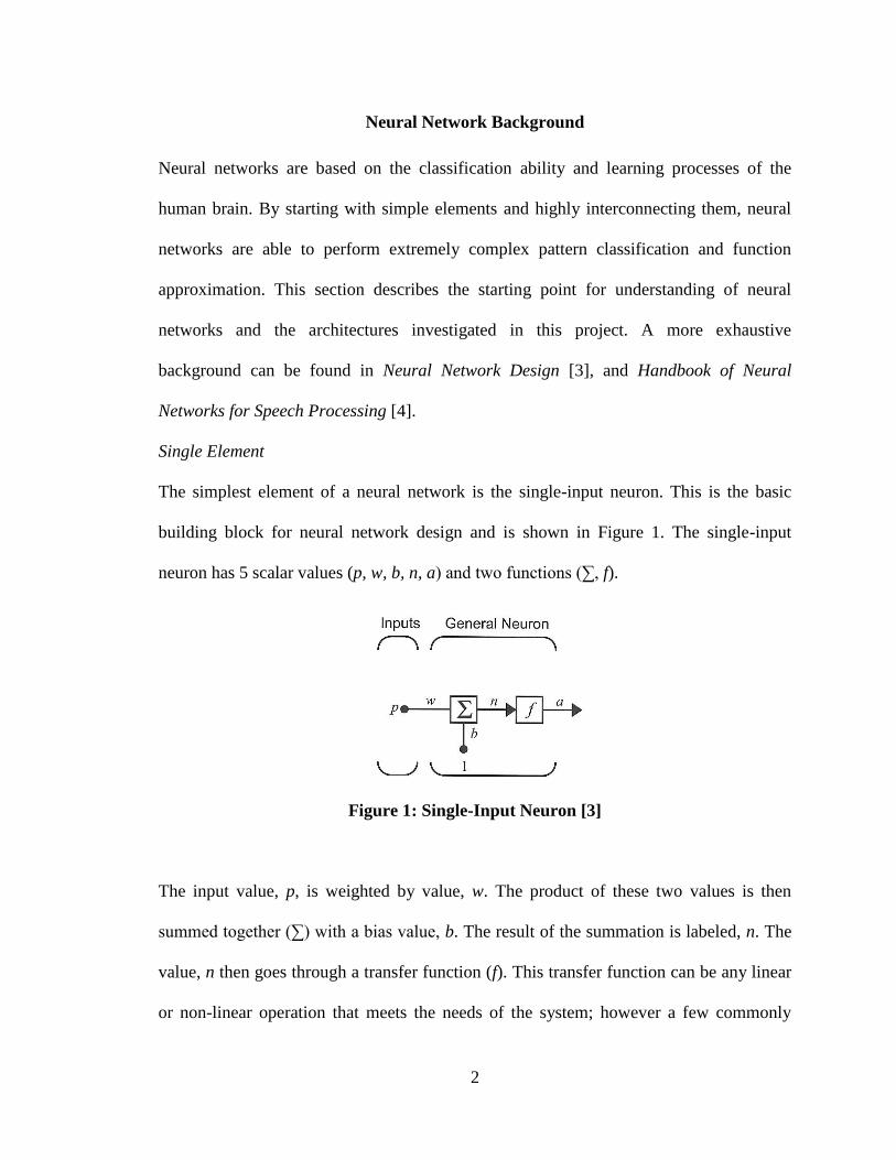
The simplest element of a neural network is the single-input neuron. This is the basic

building block for neural network design and is shown in Figure 1. The single-input

neuron has 5 scalar values (p, w, b, n, a) and two functions (∑, f).

Figure 1: Single-Input Neuron [3]

The input value, p, is weighted by value, w. The product of these two values is then

summed together (∑) with a bias value, b. The result of the summation is labeled, n. The

value, n then goes through a transfer function (f). This transfer function can be any linear

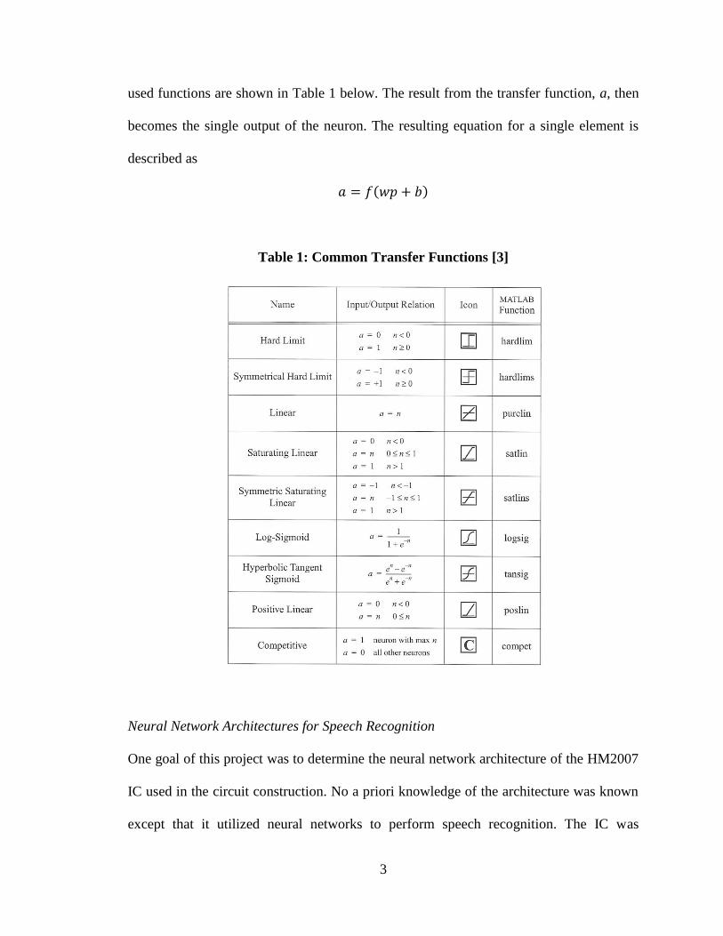
or non-linear operation that meets the needs of the system; however a few commonly

3

used functions are shown in Table 1 below. The result from the transfer function, a, then

becomes the single output of the neuron. The resulting equation for a single element is

described as

𝑎 = 𝑓 𝑤𝑝 + 𝑏

Table 1: Common Transfer Functions [3]

Neural Network Architectures for Speech Recognition

One goal of this project was to determine the neural network architecture of the HM2007

IC used in the circuit construction. No a priori knowledge of the architecture was known

except that it utilized neural networks to perform speech recognition. The IC was

4

compared against the top three most-commonly used neural network architectures for

speech recognition which are: the Multilayer Perceptron (MLP), the Time-Delay Neural

Network (TDNN), and the Recurrent Neural Network (RNN) [4]. Each of these

architectures is described in detail below.

Multilayer Perceptron (MLP)

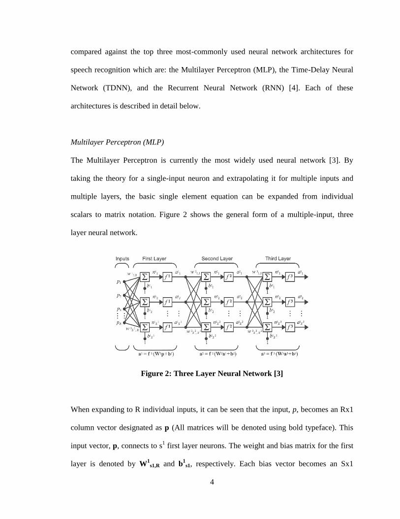
The Multilayer Perceptron is currently the most widely used neural network [3]. By

taking the theory for a single-input neuron and extrapolating it for multiple inputs and

multiple layers, the basic single element equation can be expanded from individual

scalars to matrix notation. Figure 2 shows the general form of a multiple-input, three

layer neural network.

Figure 2: Three Layer Neural Network [3]

When expanding to R individual inputs, it can be seen that the input, p, becomes an Rx1

column vector designated as p (All matrices will be denoted using bold typeface). This

input vector, p, connects to s1 first layer neurons. The weight and bias matrix for the first

layer is denoted by W1

s1,R and b1

s1, respectively. Each bias vector becomes an Sx1

5

column vector and each weight matrix has columns equal to the number of inputs into

that neuron layer and rows equal to the number of neurons in that layer. These matrices

are labeled with superscripts to denote the layer. (e.g. W3 indicates the weight matrix for

the 3rd

layer which should not be confused with raising the weight matrix to the third

power). Functions are also labeled using superscripts in the same fashion. In a single

layer, different functions can be used for each neuron, so f1 becomes a column vector of

functions to be used by each neuron for layer 1. The resulting equation for an n-input 3-

layer generic neural network is:

𝒂𝟑 = 𝒇𝟑 𝑾𝟑𝒇𝟐 𝑾𝟐𝒇𝟏 𝑾𝟏𝒑 + 𝒃𝟏 + 𝒃𝟐 + 𝒃𝟑

Studies show that a three layer network is able to solve almost any complex task

including linearly inseparable problems, and reasonably approximate any function [4].

When used in a speech recognition application, the MLP performs feature extraction on

the signal structure and creates a static vector using the signal as a whole as the MLP

input.

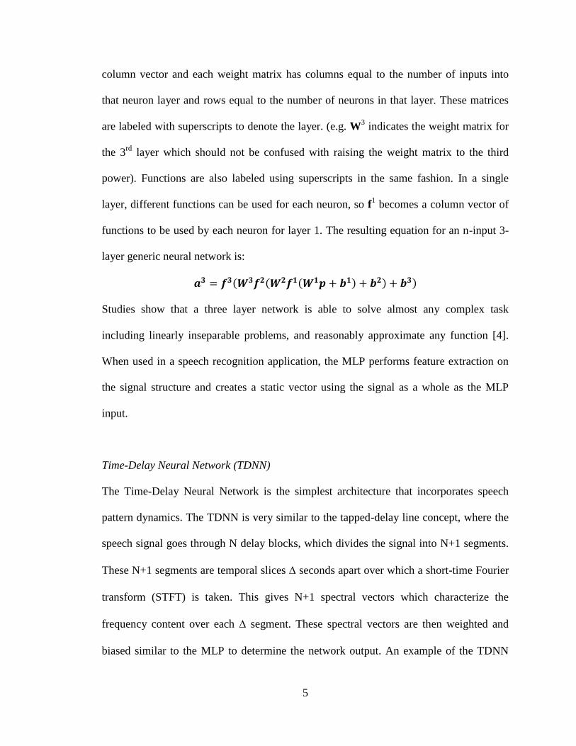
Time-Delay Neural Network (TDNN)

The Time-Delay Neural Network is the simplest architecture that incorporates speech

pattern dynamics. The TDNN is very similar to the tapped-delay line concept, where the

speech signal goes through N delay blocks, which divides the signal into N+1 segments.

These N+1 segments are temporal slices seconds apart over which a short-time Fourier

transform (STFT) is taken. This gives N+1 spectral vectors which characterize the

frequency content over each segment. These spectral vectors are then weighted and

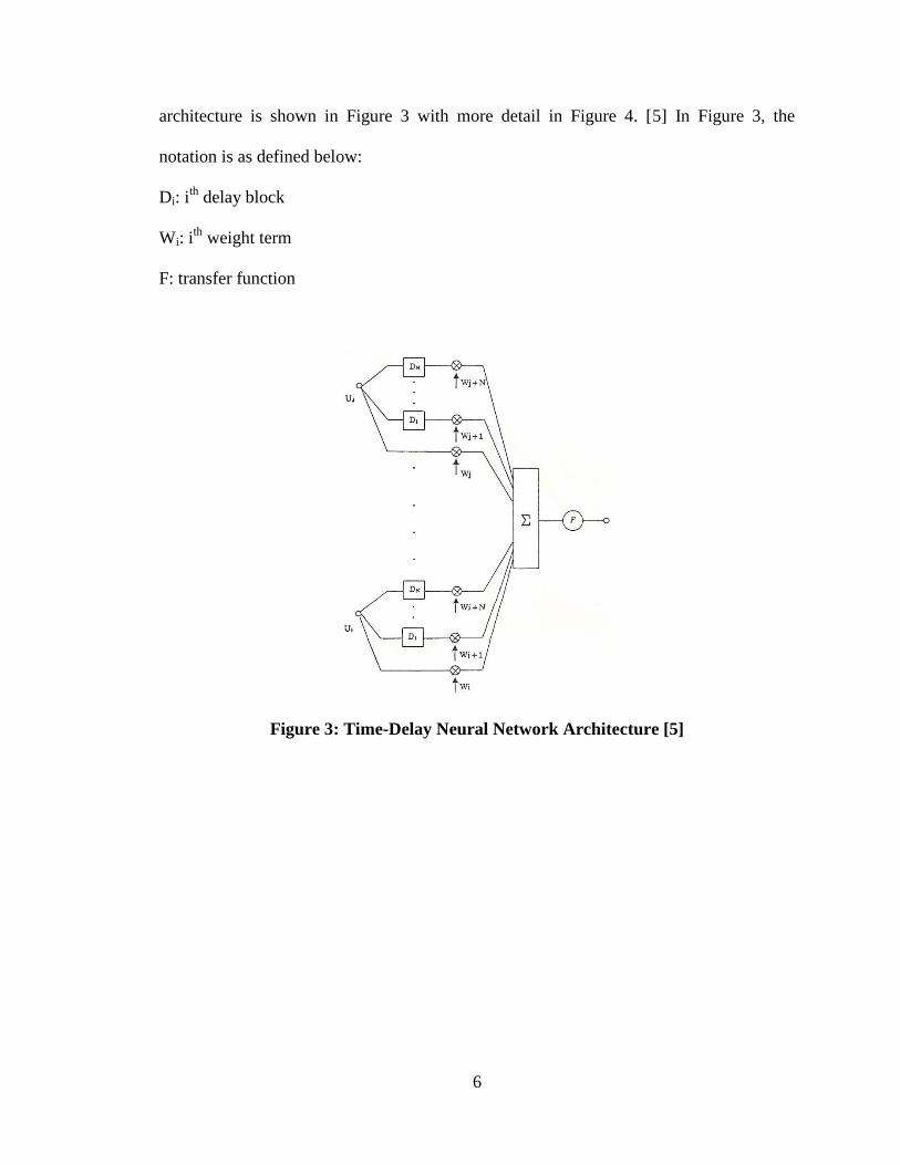
biased similar to the MLP to determine the network output. An example of the TDNN

6

architecture is shown in Figure 3 with more detail in Figure 4. [5] In Figure 3, the

notation is as defined below:

Di: ith

delay block

Wi: ith

weight term

F: transfer function

Figure 3: Time-Delay Neural Network Architecture [5]

7

Figure 4: Example of a TDNN for Recognizing /b/, /d/, and /g/ [5]

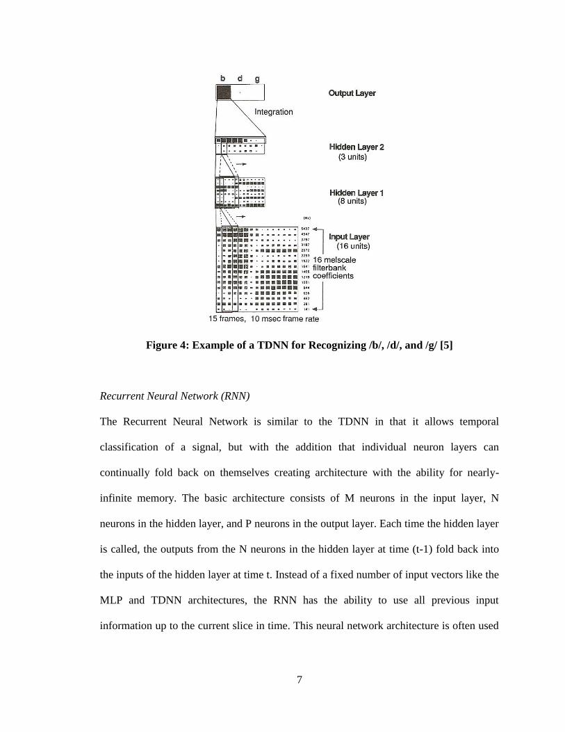
Recurrent Neural Network (RNN)

The Recurrent Neural Network is similar to the TDNN in that it allows temporal

classification of a signal, but with the addition that individual neuron layers can

continually fold back on themselves creating architecture with the ability for nearly-

infinite memory. The basic architecture consists of M neurons in the input layer, N

neurons in the hidden layer, and P neurons in the output layer. Each time the hidden layer

is called, the outputs from the N neurons in the hidden layer at time (t-1) fold back into

the inputs of the hidden layer at time t. Instead of a fixed number of input vectors like the

MLP and TDNN architectures, the RNN has the ability to use all previous input

information up to the current slice in time. This neural network architecture is often used

8

in conjunction with statistical analysis of speech to predict and classify continuous

patterns.

Figure 5: Recurrent Neural Network

Learning Rules

Each neural network must be trained with data which then creates the basis for

classifying future data. A learning rule is described as the procedure used to modify the

weights, w, and biases, b, in order to successfully classify future information that falls

outside the initial training data. Training is performed once, and then the weights are

biases are fixed. There are two broad categories to learning rules: supervised, which

means the user gives a desired target output for each element of training data, and

unsupervised, which means the user gives no target output for the training data and the

network classifies itself. Learning rules will be discussed further in the report after the

HM2007 IC architecture has been determined.

9

Speech Recognition Background

Sound is simply pressure waves that are detected by our ears and analyzed and classified

by our brains. The human voice is created by passing air from the lungs through vocal

cords. By moving the tongue, cheeks and lips words can be produced. The human voice

has a majority of its energy content between tens of Hertz and 5 kHz, but can be

approximated on the frequency spectrum from 300 Hz to 3400 Hz. Speech from an adult

male usually has a fundamental frequency (defined as the lowest tone produced by the

vocal chords) around 85-155 Hz and an adult female from 165 Hz – 255 Hz. [6]

Although these fundamental frequencies fall below the 300 Hz lower bound, harmonics

occur at integer multiples of the fundamental frequency giving the impression of actually

hearing the fundamental frequency even though it is below the lower bound of the

approximated range [6]. Speech recognition is performed virtually seamlessly by the

original neural network, our brain, which processes and classifies sounds and words in a

variety of complex environments: with background noise, with words blended together in

continuous speech, with accents, and without regard to who the speaker is.

Trying to perform the same tasks with neural networks based in software or hardware

becomes a difficult undertaking, but once speech recognition is successfully implemented

it can be used for controlling applications, performing data entry, interfacing with

computers, or a host of other ways.

Speech is utilized in circuits the following way: the acoustic pressure wave goes through

a transducer inside a microphone or telephone and converts it from a pressure wave to an

electrical signal. “A speech-wave is a one-dimensional signal having temporal structure.

The signal can be considered a combination of different frequency sine-waves, and its

10

acoustical characteristics are determined by the frequency, energy (amplitude), and phase

of each component sine-wave. However, for speech recognition, a speech signal is

usually converted to a three-dimensional, time-frequency-energy feature pattern that is

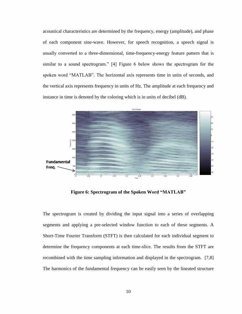
similar to a sound spectrogram.” [4] Figure 6 below shows the spectrogram for the

spoken word “MATLAB”. The horizontal axis represents time in units of seconds, and

the vertical axis represents frequency in units of Hz. The amplitude at each frequency and

instance in time is denoted by the coloring which is in units of decibel (dB).

Figure 6: Spectrogram of the Spoken Word “MATLAB”

The spectrogram is created by dividing the input signal into a series of overlapping

segments and applying a pre-selected window function to each of these segments. A

Short-Time Fourier Transform (STFT) is then calculated for each individual segment to

determine the frequency components at each time-slice. The results from the STFT are

recombined with the time sampling information and displayed in the spectrogram. [7,8]

The harmonics of the fundamental frequency can be easily seen by the lineated structure

11

present in the spectrogram. For this signal, the fundamental frequency was approximately

231 Hz. Since this word was spoken by a female, it falls within the appropriate range.

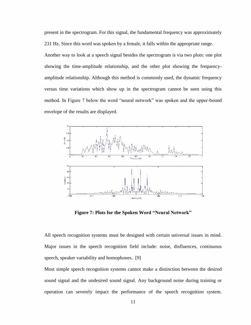
Another way to look at a speech signal besides the spectrogram is via two plots: one plot

showing the time-amplitude relationship, and the other plot showing the frequency-

amplitude relationship. Although this method is commonly used, the dynamic frequency

versus time variations which show up in the spectrogram cannot be seen using this

method. In Figure 7 below the word “neural network” was spoken and the upper-bound

envelope of the results are displayed.

Figure 7: Plots for the Spoken Word “Neural Network”

All speech recognition systems must be designed with certain universal issues in mind.

Major issues in the speech recognition field include: noise, disfluences, continuous

speech, speaker variability and homophones. [9]

Most simple speech recognition systems cannot make a distinction between the desired

sound signal and the undesired sound signal. Any background noise during training or

operation can severely impact the performance of the speech recognition system.

12

Disfluences are parts of human speech that often go unnoticed by people. They are slips

of the tongue, hesitations in speech, and utterances such as “uhh” and “um”. In a speech

recognition system, these parts of speech will try to be classified just like any other part

of speech, which can often lead to errors or misclassifications. Natural human speech

happens in a continuous manner where words blend together and are not always

separated by a distinguishable pause. This poses a problem for speech recognition

systems in determining the boundaries of a word and matching them to the trained

patterns. Speech recognition systems can be classified into three broad categories:

isolated word speech recognition, connected word speech recognition, or continuous

speech recognition. In isolated word speech recognition, each word must have distinct

pauses before and after the word. These are usually used for command type applications

where relatively short words or “commands” cause some sort of action to happen.

Connected word speech recognition is similar to isolated word speech recognition, but

the “word” can be a single word or a phrase of words that fit within the allowable time

window, and in continuous speech recognition the system recognizes words and phrases

in ordinary spoken language without the user making any adjustments from normal

conversation.

Speaker variability occurs is multiple ways. There is variability in the same word when

spoken multiple times even by the same person. Each distinct waveform will look slightly

different in timing, amplitude and frequency. These variations must be taken into account

to ensure that the criteria for word matching are not so stringent that these variations

cause the word to be unknown or misclassified. Speaking conditions also cause

variability; for example the spoken word “Eject” used to control a cockpit function will

13

sound much different (and the resulting waveform will look much different) when spoken

in a non-stressed condition versus a condition of extreme excitement. Also, the most

familiar form of speaker variability comes simply from different speakers. The signal

features of a spoken word look much different depending on the gender of the speaker,

the accent of the speaker, and the age and voice type of the speaker. All these categories

cause extreme variability even in the case of a single spoken word.

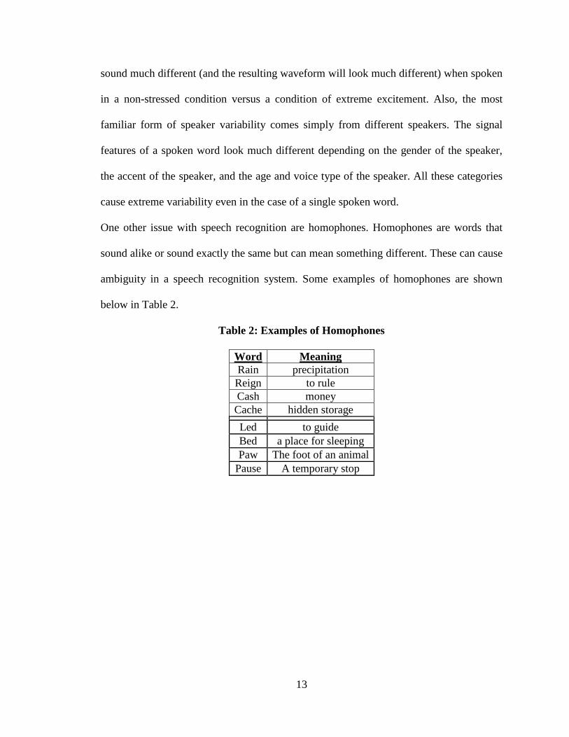
One other issue with speech recognition are homophones. Homophones are words that

sound alike or sound exactly the same but can mean something different. These can cause

ambiguity in a speech recognition system. Some examples of homophones are shown

below in Table 2.

Table 2: Examples of Homophones

Word Meaning

Rain precipitation

Reign to rule

Cash money

Cache hidden storage

Led to guide

Bed a place for sleeping

Paw The foot of an animal

Pause A temporary stop

14

Circuit Construction

Most neural network systems are designed using software. The ease of manipulating data

and changing the architecture make software a popular choice. An often unlooked at side

of neural networks is when they are created using hardware. The first goal of this project

was to create a circuit implementing neural network technology that utilized stand-alone

hardware to perform the functions instead of the more commonly used software. The

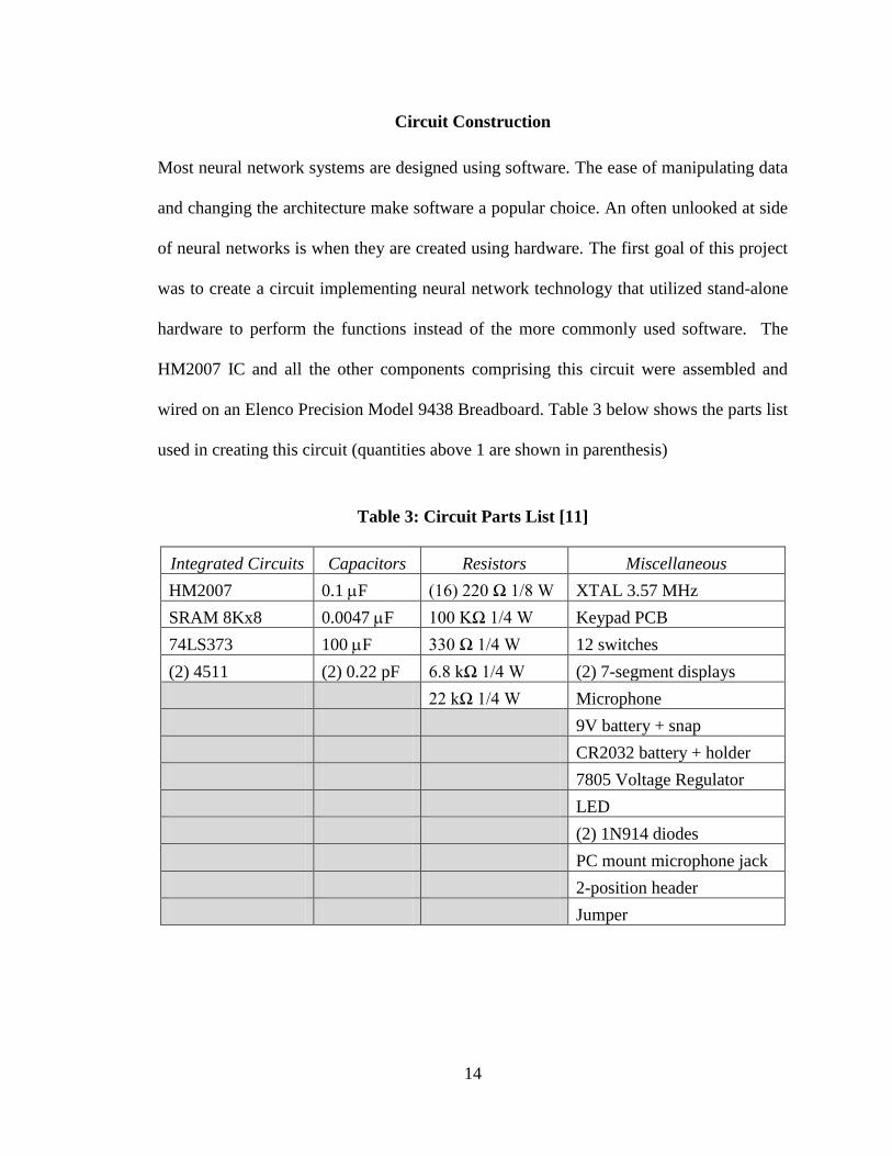
HM2007 IC and all the other components comprising this circuit were assembled and

wired on an Elenco Precision Model 9438 Breadboard. Table 3 below shows the parts list

used in creating this circuit (quantities above 1 are shown in parenthesis)

Table 3: Circuit Parts List [11]

Integrated Circuits Capacitors Resistors Miscellaneous

HM2007 0.1 F (16) 220 Ω 1/8 W XTAL 3.57 MHz

SRAM 8Kx8 0.0047 F 100 KΩ 1/4 W Keypad PCB

74LS373 100 F 330 Ω 1/4 W 12 switches

(2) 4511 (2) 0.22 pF 6.8 kΩ 1/4 W (2) 7-segment displays

22 kΩ 1/4 W Microphone

9V battery + snap

CR2032 battery + holder

7805 Voltage Regulator

LED

(2) 1N914 diodes

PC mount microphone jack

2-position header

Jumper

15

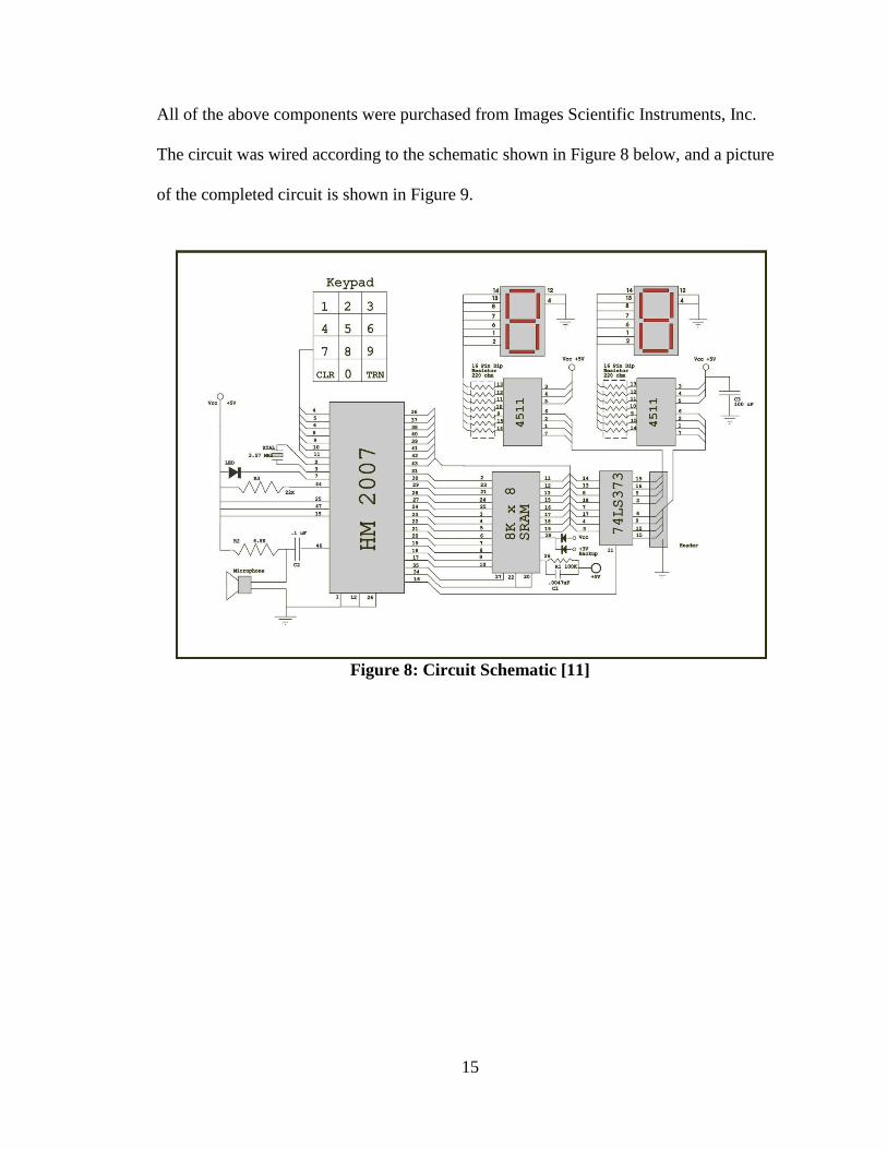
All of the above components were purchased from Images Scientific Instruments, Inc.

The circuit was wired according to the schematic shown in Figure 8 below, and a picture

of the completed circuit is shown in Figure 9.

Figure 8: Circuit Schematic [11]

16

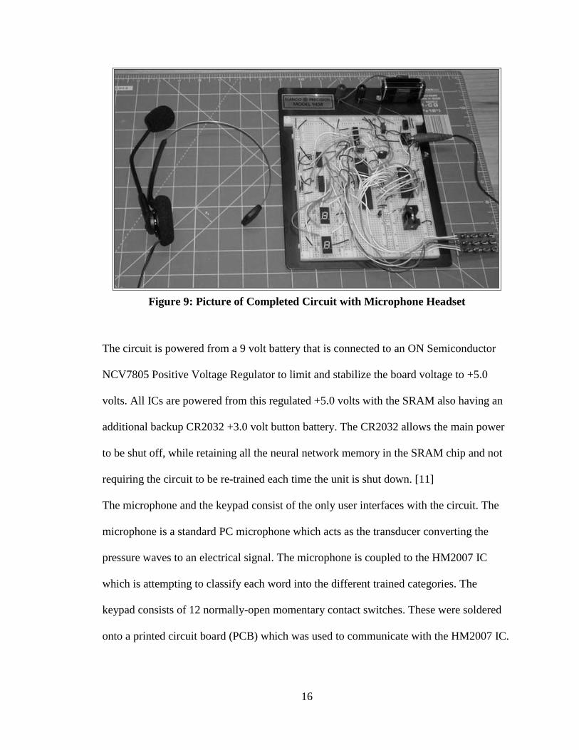
Figure 9: Picture of Completed Circuit with Microphone Headset

The circuit is powered from a 9 volt battery that is connected to an ON Semiconductor

NCV7805 Positive Voltage Regulator to limit and stabilize the board voltage to +5.0

volts. All ICs are powered from this regulated +5.0 volts with the SRAM also having an

additional backup CR2032 +3.0 volt button battery. The CR2032 allows the main power

to be shut off, while retaining all the neural network memory in the SRAM chip and not

requiring the circuit to be re-trained each time the unit is shut down. [11]

The microphone and the keypad consist of the only user interfaces with the circuit. The

microphone is a standard PC microphone which acts as the transducer converting the

pressure waves to an electrical signal. The microphone is coupled to the HM2007 IC

which is attempting to classify each word into the different trained categories. The

keypad consists of 12 normally-open momentary contact switches. These were soldered

onto a printed circuit board (PCB) which was used to communicate with the HM2007 IC.

17

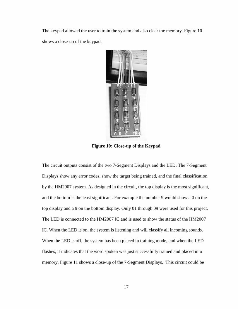
The keypad allowed the user to train the system and also clear the memory. Figure 10

shows a close-up of the keypad.

Figure 10: Close-up of the Keypad

The circuit outputs consist of the two 7-Segment Displays and the LED. The 7-Segment

Displays show any error codes, show the target being trained, and the final classification

by the HM2007 system. As designed in the circuit, the top display is the most significant,

and the bottom is the least significant. For example the number 9 would show a 0 on the

top display and a 9 on the bottom display. Only 01 through 09 were used for this project.

The LED is connected to the HM2007 IC and is used to show the status of the HM2007

IC. When the LED is on, the system is listening and will classify all incoming sounds.

When the LED is off, the system has been placed in training mode, and when the LED

flashes, it indicates that the word spoken was just successfully trained and placed into

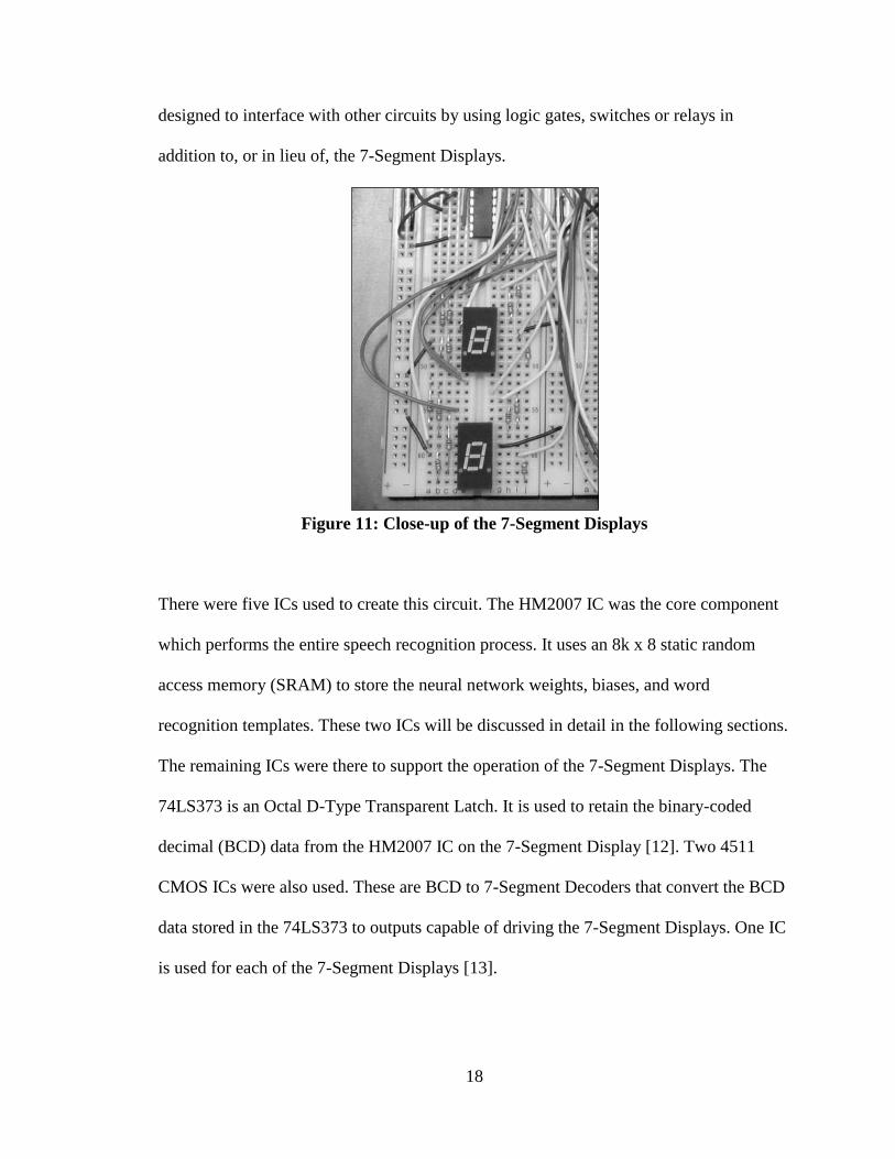
memory. Figure 11 shows a close-up of the 7-Segment Displays. This circuit could be

18

designed to interface with other circuits by using logic gates, switches or relays in

addition to, or in lieu of, the 7-Segment Displays.

Figure 11: Close-up of the 7-Segment Displays

There were five ICs used to create this circuit. The HM2007 IC was the core component

which performs the entire speech recognition process. It uses an 8k x 8 static random

access memory (SRAM) to store the neural network weights, biases, and word

recognition templates. These two ICs will be discussed in detail in the following sections.

The remaining ICs were there to support the operation of the 7-Segment Displays. The

74LS373 is an Octal D-Type Transparent Latch. It is used to retain the binary-coded

decimal (BCD) data from the HM2007 IC on the 7-Segment Display [12]. Two 4511

CMOS ICs were also used. These are BCD to 7-Segment Decoders that convert the BCD

data stored in the 74LS373 to outputs capable of driving the 7-Segment Displays. One IC

is used for each of the 7-Segment Displays [13].

19

Operation of the Circuit

As far as hardware configuration is concerned, there is only a single area of adjustment.

By pulling pin 13 high on the HM2007 IC, the maximum word length is set to 1.92

seconds and a 20 word capability (instead of a 0.96 sec word length and 40 word

capability when pulled low). This is the configuration used throughout the entire report.

The smaller word capability was used since the manual for the HM2007 stated that this

configuration provided better accuracy than the alternative setup. [11]

To place the circuit in training mode, a number is pressed on the keypad representing a

specific target class index (i.e. 0-1). A target class index is defined as the desired outcome

on the display. The total number of class indices programmed can be anywhere from 1 to

20. The LED now turns off indicating that the circuit is ready to train. The TRN button is

pressed on the keypad and the word for slot 01 is spoken. The LED then blinks indicating

the word had been trained. This can continue for as many slots as desired up to the full

capacity of the system. Once training was completed and the LED remained illuminated,

the system was continuously listening for the microphone input and attempting to classify

the words it heard.

A single class index could be cleared by pressing the slot number on the keypad and then

CLR (i.e. to clear slot 4, 0-4-CLR). The entire memory could be cleared by pressing 9-9-

CLR. The 7-Segment Display showed each number as it cleared that slot.

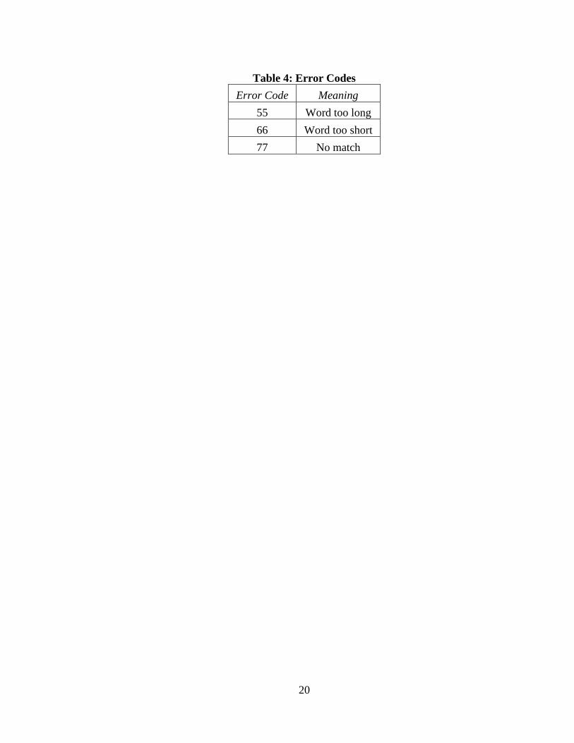
If there were any problems with the classification, error codes were displayed on the 7-

Segment Display. The error codes are shown below in Table 4.

20

Table 4: Error Codes

Error Code Meaning

55 Word too long

66 Word too short

77 No match

21

Architecture Testing & Determination

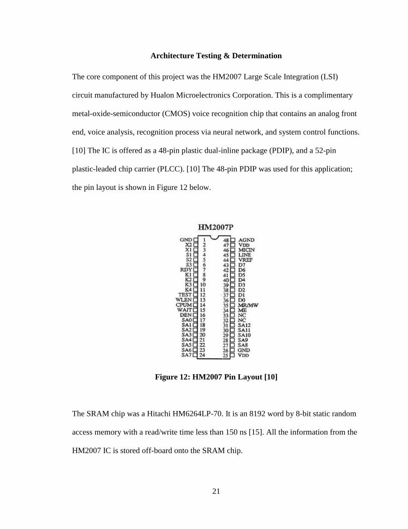
The core component of this project was the HM2007 Large Scale Integration (LSI)

circuit manufactured by Hualon Microelectronics Corporation. This is a complimentary

metal-oxide-semiconductor (CMOS) voice recognition chip that contains an analog front

end, voice analysis, recognition process via neural network, and system control functions.

[10] The IC is offered as a 48-pin plastic dual-inline package (PDIP), and a 52-pin

plastic-leaded chip carrier (PLCC). [10] The 48-pin PDIP was used for this application;

the pin layout is shown in Figure 12 below.

Figure 12: HM2007 Pin Layout [10]

The SRAM chip was a Hitachi HM6264LP-70. It is an 8192 word by 8-bit static random

access memory with a read/write time less than 150 ns [15]. All the information from the

HM2007 IC is stored off-board onto the SRAM chip.

22

The second goal of this project was to determine the neural network architecture used for

speech recognition in the HM2007 IC. As mentioned previously the three most common

neural network architectures used for speech recognition are: MLP, TDNN, and RNN.

An extensive search of the literature pertaining to the HM2007 IC was conducted, but

nothing pertaining to the architecture was found. There were, however, some papers

describing some very interesting applications created with this chip ranging from the

novel (talking toaster, control of a toy robotic arm) [18,19] to the useful (voice activated

wheelchair, advanced rescue vision system). [20,21] A series of tests was designed to

narrow down the architecture and parameters of the neural network system. The circuit

was interfaced with standard computer speakers generating unique sounds produced by

custom MATLAB code created for this experimentation. The entire code can be found in

APPENDIX A.

The first test series determined whether the chip operated using time-dependent

parameters, or only static analysis of the entire signal as a whole. Two tests were

performed in this phase: one observing signal amplitude versus time, and one observing

frequency versus time. The amplitude versus time test was conducted by importing the

spoken word “neural network” into MATLAB. This audio file was converted into two

files, y1 which was a mono playback of the original signal, and y2, which was a reversed

version of y1. These signals only differed in the timing of their amplitudes. Their

frequency spectrum was intrinsically identical for the whole signal. The circuit was then

trained into class indices 01 and 02 using these two signals. The hypothesis was that if

amplitude versus time was a feature of the neural network, then the circuit would be able

to distinguish and correctly classify the two similar signals. Upon playback these signals

23

were always distinguishable and were correctly classified. The second test in this phase

was conducted likewise, but this time observing any frequency versus time dependence.

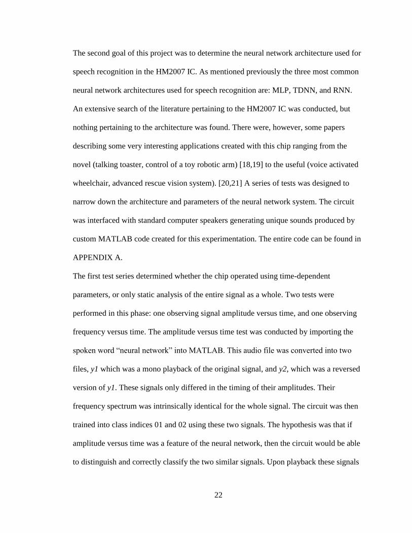
Two simple tones were generated in MATLAB, one at f1=1000 Hz and the other at

f2=2000 Hz. They were then concatenated into a 1 second signal with each tone lasting

0.5 seconds. The first signal (X1) played the order f1, f2 and the second file (X2) played

the order f2,f1. Both of these signals look the same when analyzing the frequency

spectrum of the whole signal and had identical amplitudes, but different if taking the

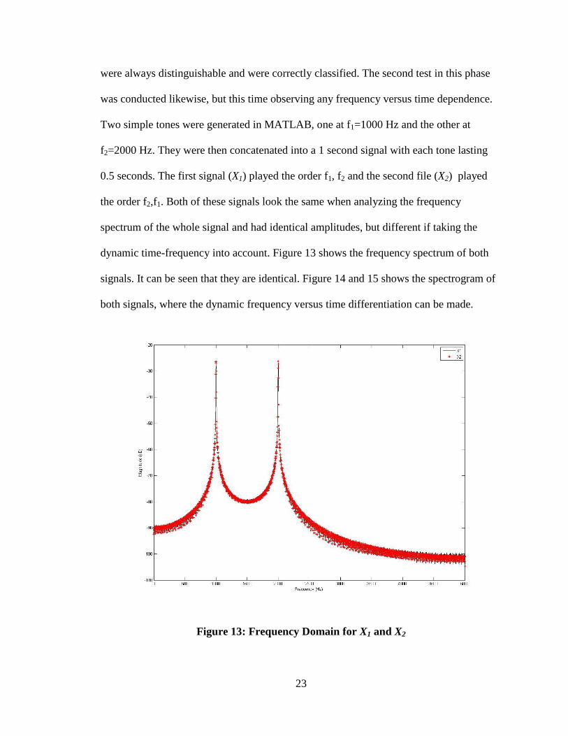
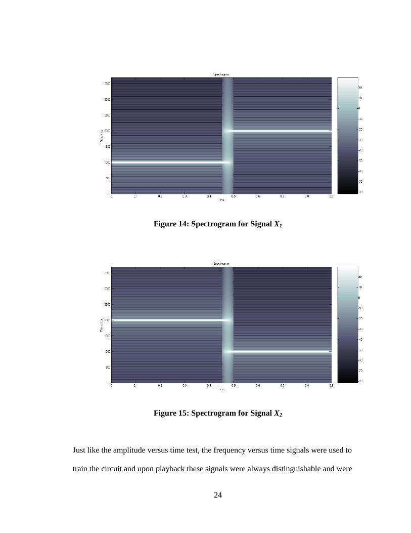
dynamic time-frequency into account. Figure 13 shows the frequency spectrum of both

signals. It can be seen that they are identical. Figure 14 and 15 shows the spectrogram of

both signals, where the dynamic frequency versus time differentiation can be made.

Figure 13: Frequency Domain for X1 and X2

24

Figure 14: Spectrogram for Signal X1

Figure 15: Spectrogram for Signal X2

Just like the amplitude versus time test, the frequency versus time signals were used to

train the circuit and upon playback these signals were always distinguishable and were

25

correctly classified. This test phase clearly demonstrated that the dynamic time-effects

were being recognized and used as feature inputs to the HM2007 neural network

architecture. This eliminated the possibility of an MLP architecture.

Between the remaining time-dependent architectures, by inspection the TDNN was the

best fit. RNN architecture has the disadvantage in that it requires many neurons and

excessive computation time [3], and the “weights are often on the order of 10,000 to 2

million and training data vectors are often in the order of 1 million to 100 million” [4].

For a system with a 64 kbit memory, this is not possible. Also the RNN architecture is

often used for higher-fidelity continuous speech recognition systems which would be an

excessive architecture for this connected-word style system. The TDNN is essentially a

RNN architecture with limited connections. This speeds up training time and reduces

memory requirements [14]. The TDNN works by breaking down the data into N+1 time

segments (using N delay blocks) with lengths of seconds. Each of these segments has a

STFT performed to determine the dynamic frequency content of the entire signal. The

next three tests were performed to determine the number of delay blocks (N), the time

segment length (), the upper and lower frequency bounds used as features, and the

resolution of the frequency measurements.

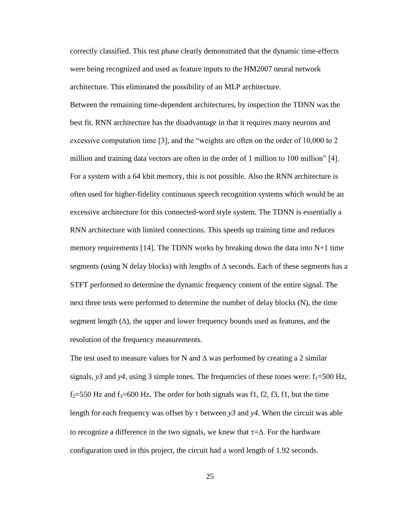
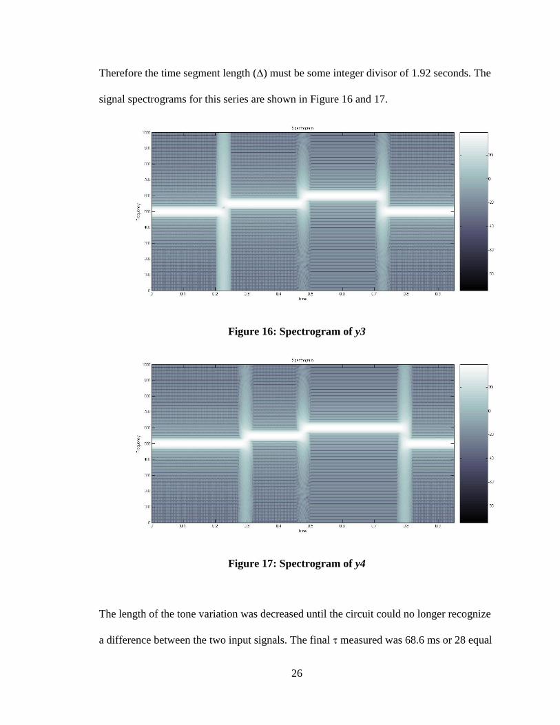
The test used to measure values for N and was performed by creating a 2 similar

signals, y3 and y4, using 3 simple tones. The frequencies of these tones were: f1=500 Hz,

f2=550 Hz and f3=600 Hz. The order for both signals was f1, f2, f3, f1, but the time

length for each frequency was offset by between y3 and y4. When the circuit was able

to recognize a difference in the two signals, we knew that =. For the hardware

configuration used in this project, the circuit had a word length of 1.92 seconds.

26

Therefore the time segment length () must be some integer divisor of 1.92 seconds. The

signal spectrograms for this series are shown in Figure 16 and 17.

Figure 16: Spectrogram of y3

Figure 17: Spectrogram of y4

The length of the tone variation was decreased until the circuit could no longer recognize

a difference between the two input signals. The final measured was 68.6 ms or 28 equal

27

time segments of the 1.92 second word length. Therefore we estimate that the HM2007

neural network architecture utilized a =68.6 ms which requires a total of N=27 delay

blocks.

The next test was executed to measure the upper and lower frequency limits used as

features in the neural network architecture. A simple tone was produced in MATLAB and

increased in frequency until the circuit could no longer recognize the signal; similarly, the

lower limit was measured by decreasing the tone frequency until the circuit could no

longer recognize the signal. The measured bounds were: FLower Limit = 400 Hz and FUpper

Limit = 2000 Hz. This meant that the Analog-to-Digital Converter (ADC) was sampling

this microphone input at least 4000 times per second to meet the Nyquist Sampling Rate

and ensure there was no aliasing.

The final test completed was to determine the frequency resolution of the HM2007 IC. A

tone was generated at 1000 Hz and a second tone was generated at (1000+) Hz. The

resolution, was initially set to 300 Hz and then lowered until the circuit could no longer

distinguish between the two tones. The final measured value was 25 Hz. Since:

(𝑈𝑝𝑝𝑒𝑟 𝐿𝑖𝑚𝑖𝑡 − 𝐿𝑜𝑤𝑒𝑟 𝐿𝑖𝑚𝑖𝑡)

=

(2000 − 400)

25= 64

This indicated that a 64-point STFT is calculated at each time segment in the TDNN.

Taking the results of all these tests together, the final HM2007 neural network

architecture can be estimated. It was determined that the IC best fits the general TDNN

architecture. As further testing was performed, this was confirmed and the parameters of

28

the TDNN were measured. The results imply that there are 64 neurons in the input layer

corresponding to the 64 separate 25 Hz filter “bins” that cover the frequency spectrum

from 400 Hz to 2000 Hz. The input signal passes through 27 delay blocks with a delay

time of 68.6 ms repeating the same 64 neurons after each delay. These 64 neurons then

connect with an unknown number of neurons in an unknown number of hidden layers

which then connect to an output layer with 8 neurons using the Hard Limit transfer

function (since the only possible outputs are 0 or 1 from the digital circuit). These 8

neurons correspond to the binary coded decimal (BCD) output of class index 01 through

20 (since there is the possibility of a 20 word library for this configuration). The 8 output

neurons correspond with the D0-D7 output of the HM2007 IC (pins 36-43) which

controls the two 7-Segment Display outputs. Outputs D4-D7 make up the BCD for

display “A” which consists of the values 0-2 (where 3-9 are unused), and outputs D0-D3

make up the BCD for display “B” consisting of the numbers 0-9. Essentially, the

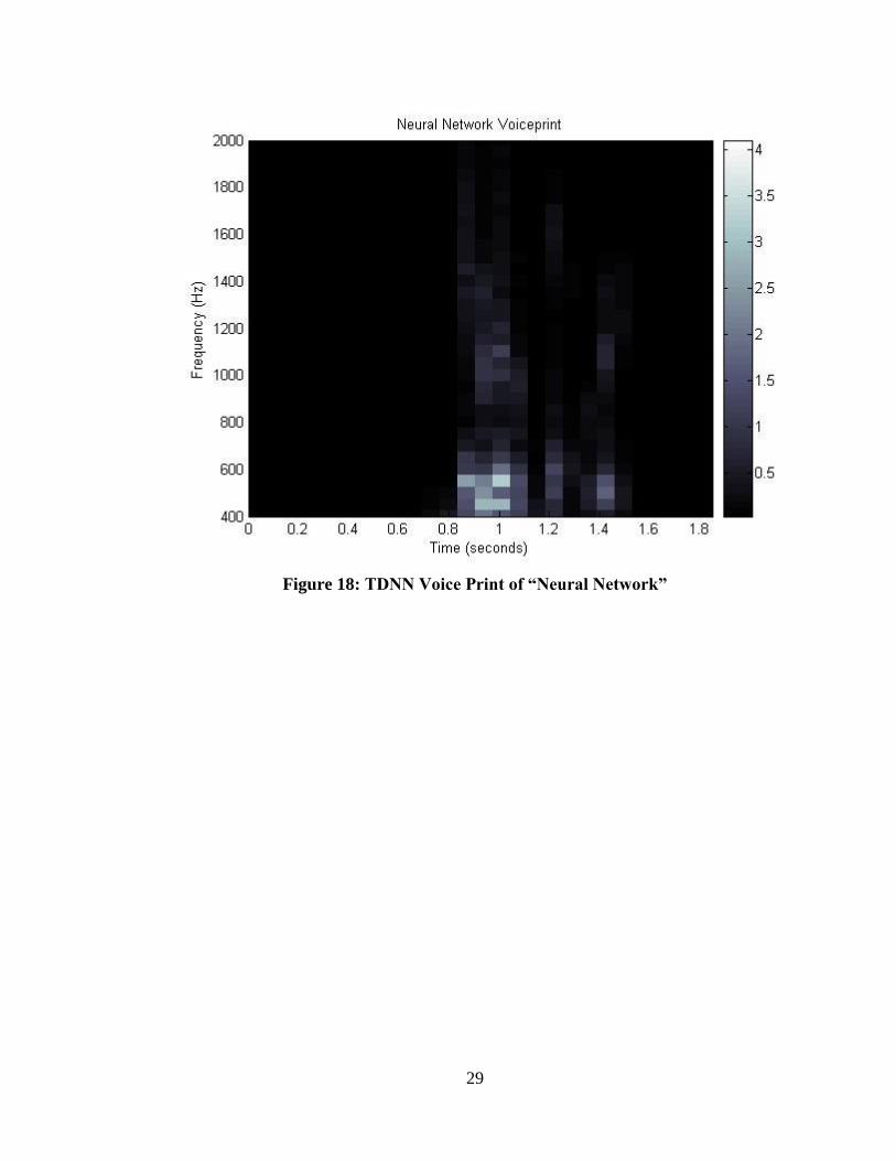
HM2007 IC takes a data template or “voiceprint” of the sampled speech signal which can

be graphically represented like Figure 18 which consists of the spoken word “neural

network” broken down into 28 segments in time (each 68.3 ms in duration), for each of

which a 64 point STFT is calculated with 8-bit quantization. A detailed explanation of the

MATLAB process to obtain Figure 18 can be found in APPENDIX B. The data from

this voiceprint is then used to train the weights and biases for the programmed target

class. Due to the operation of the circuit, the learning style is supervised. Because the

circuit is trained one class at a time, the circuit is not optimized which means that the

border for classification could be right up against the hyper-dimensional geometric edge

potentially causing misclassification.

29

Figure 18: TDNN Voice Print of “Neural Network”

30

Performance Testing

Various tests were performed on the completed speech recognition circuit to investigate

its robustness and to characterize performance. The first set of tests looked at the

recognition accuracy. This is the most important parameter in any speech recognition

system because it tests the whole system from start to end. In some extreme cases the

system can become unusable or even dangerous when the recognition accuracy

percentage drops too low. In a study of speech recognition in high-performance fighter

aircraft where speech recognition was used for controlling flight displays, setting radio

frequencies, and weapon release parameters it was determined that a high recognition

accuracy (correct classification above 95%) was the most critical factor in making the

system useful. When the recognition accuracy was below this, the pilots stopped using

the system. [16]. In this first series of tests, recognition errors either came from receiving

an error code when a word was spoken or when it was misclassified as another trained

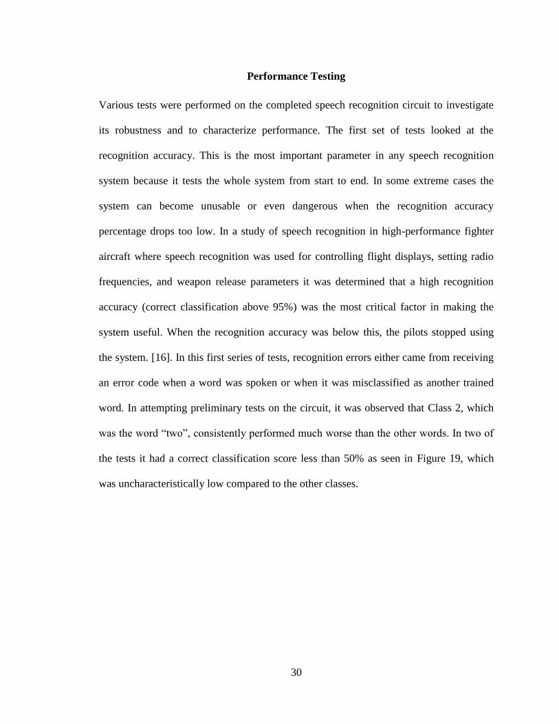
word. In attempting preliminary tests on the circuit, it was observed that Class 2, which

was the word “two”, consistently performed much worse than the other words. In two of

the tests it had a correct classification score less than 50% as seen in Figure 19, which

was uncharacteristically low compared to the other classes.

31

Figure 19: Preliminary Recognition Accuracy

It could be that this word was too short and contained too little structure to adequately

train the system to recognize the word. Class 2 did receive an error code 66 “Word too

short” 14% of the time, the other 24% it was misclassified as class index 3, the word

“Three”. It was then determined to change the word classification from “one”, “two”,

“three”, etc to those of aircraft in the Air Force inventory. This was chosen to increase the

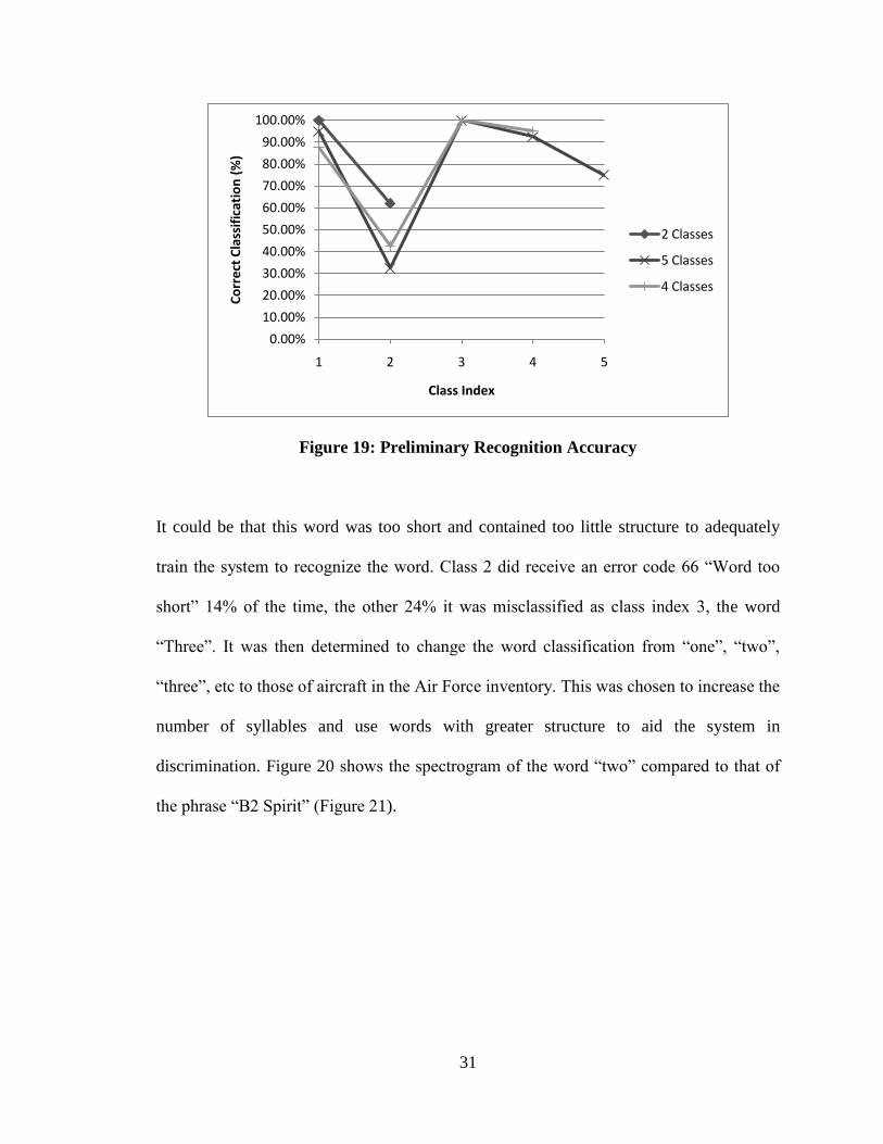
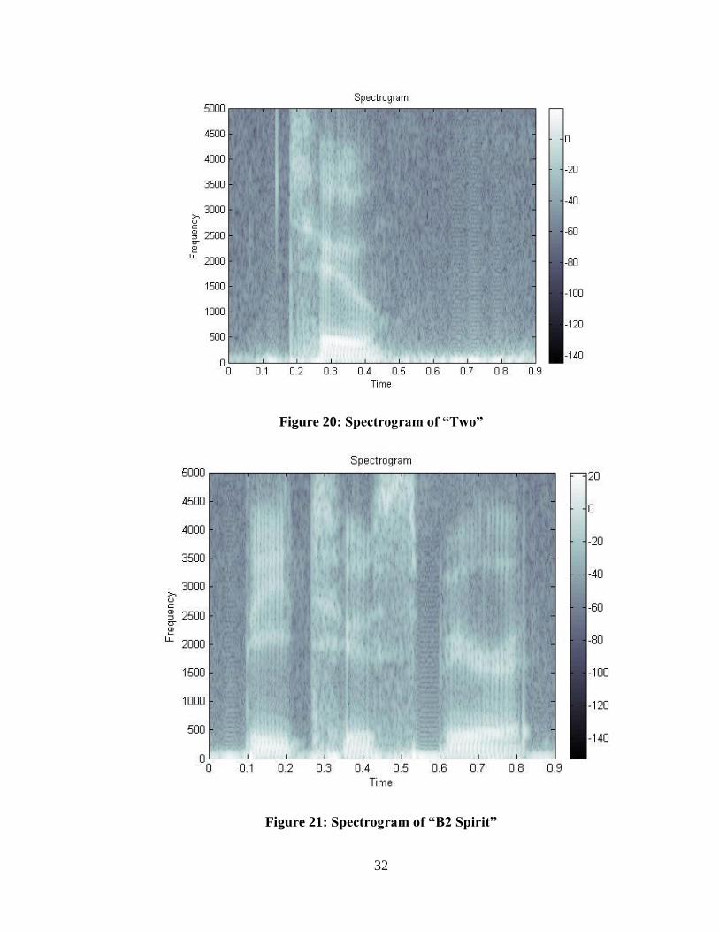
number of syllables and use words with greater structure to aid the system in

discrimination. Figure 20 shows the spectrogram of the word “two” compared to that of

the phrase “B2 Spirit” (Figure 21).

0.00%

10.00%

20.00%

30.00%

40.00%

50.00%

60.00%

70.00%

80.00%

90.00%

100.00%

1 2 3 4 5

Co

rre

ct C

lass

ific

atio

n (

%)

Class Index

2 Classes

5 Classes

4 Classes

32

Figure 20: Spectrogram of “Two”

Figure 21: Spectrogram of “B2 Spirit”

33

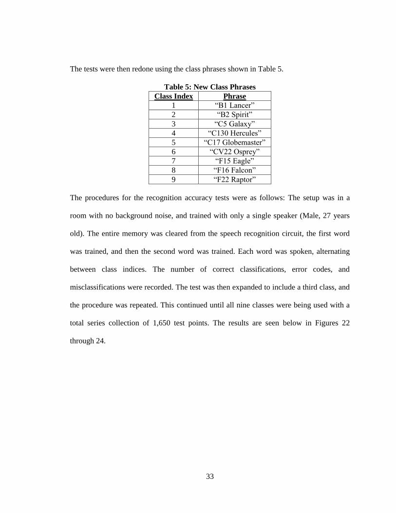
The tests were then redone using the class phrases shown in Table 5.

Table 5: New Class Phrases

Class Index Phrase

1 “B1 Lancer”

2 “B2 Spirit”

3 “C5 Galaxy”

4 “C130 Hercules”

5 “C17 Globemaster”

6 “CV22 Osprey”

7 “F15 Eagle”

8 “F16 Falcon”

9 “F22 Raptor”

The procedures for the recognition accuracy tests were as follows: The setup was in a

room with no background noise, and trained with only a single speaker (Male, 27 years

old). The entire memory was cleared from the speech recognition circuit, the first word

was trained, and then the second word was trained. Each word was spoken, alternating

between class indices. The number of correct classifications, error codes, and

misclassifications were recorded. The test was then expanded to include a third class, and

the procedure was repeated. This continued until all nine classes were being used with a

total series collection of 1,650 test points. The results are seen below in Figures 22

through 24.

34

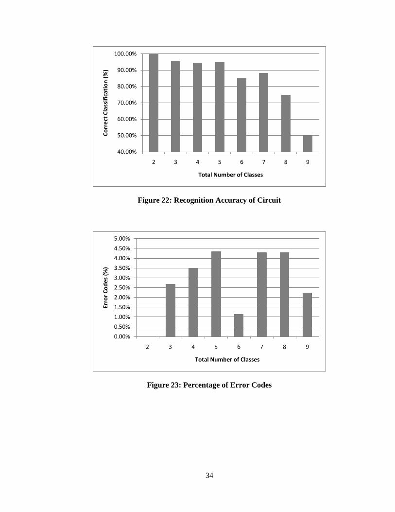
Figure 22: Recognition Accuracy of Circuit

Figure 23: Percentage of Error Codes

40.00%

50.00%

60.00%

70.00%

80.00%

90.00%

100.00%

2 3 4 5 6 7 8 9

Co

rre

ct C

lass

ific

atio

n (

%)

Total Number of Classes

0.00%

0.50%

1.00%

1.50%

2.00%

2.50%

3.00%

3.50%

4.00%

4.50%

5.00%

2 3 4 5 6 7 8 9

Erro

r C

od

es

(%)

Total Number of Classes

35

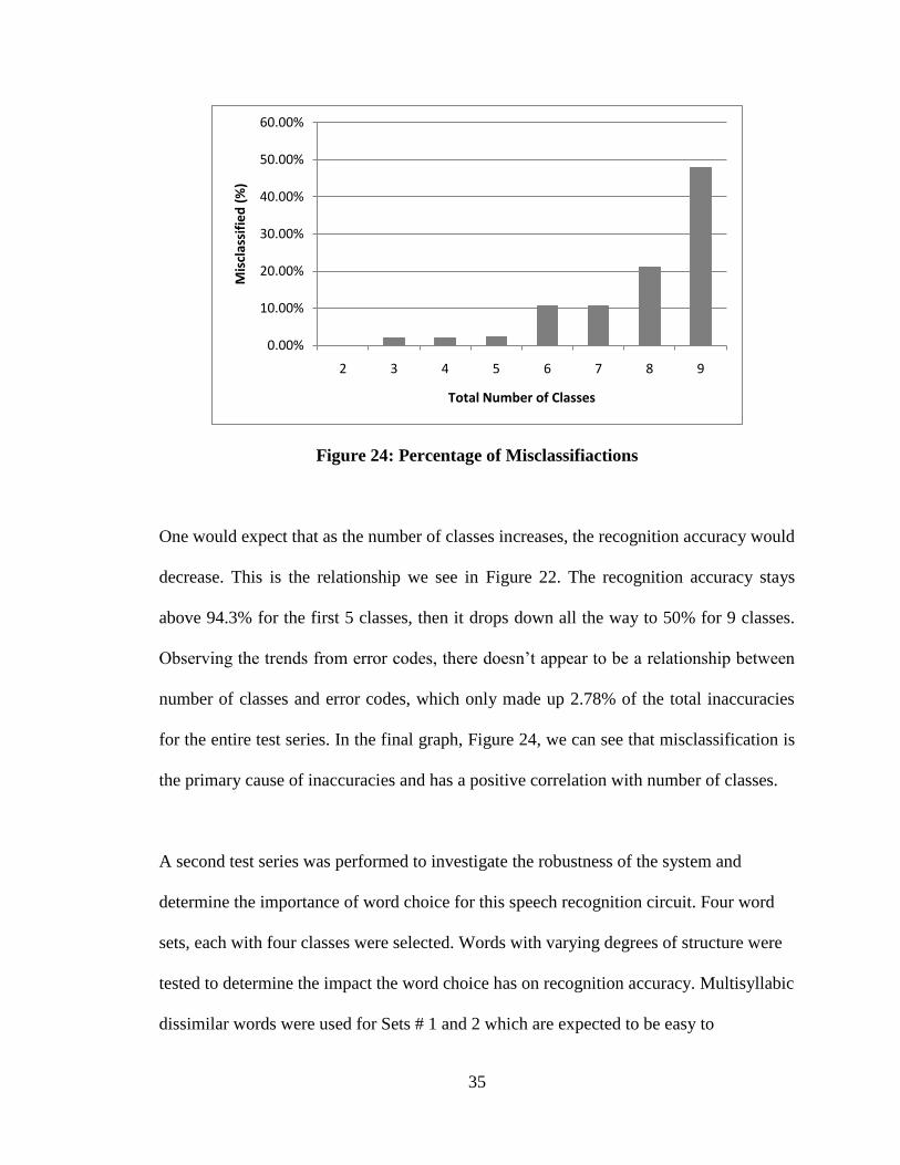
Figure 24: Percentage of Misclassifiactions

One would expect that as the number of classes increases, the recognition accuracy would

decrease. This is the relationship we see in Figure 22. The recognition accuracy stays

above 94.3% for the first 5 classes, then it drops down all the way to 50% for 9 classes.

Observing the trends from error codes, there doesn’t appear to be a relationship between

number of classes and error codes, which only made up 2.78% of the total inaccuracies

for the entire test series. In the final graph, Figure 24, we can see that misclassification is

the primary cause of inaccuracies and has a positive correlation with number of classes.

A second test series was performed to investigate the robustness of the system and

determine the importance of word choice for this speech recognition circuit. Four word

sets, each with four classes were selected. Words with varying degrees of structure were

tested to determine the impact the word choice has on recognition accuracy. Multisyllabic

dissimilar words were used for Sets # 1 and 2 which are expected to be easy to

0.00%

10.00%

20.00%

30.00%

40.00%

50.00%

60.00%

2 3 4 5 6 7 8 9

Mis

clas

sifi

ed

(%

)

Total Number of Classes

36

distinguish, and homophones were specifically used in Set #3 and Set #4 which are

expected to be difficult to distinguish. All words came from a set of standardized lists

used in testing auditory deficiencies in humans. Sets #1 and 2 came from the

Multisyllabic Lexical Neighborhood Test (Kirk – 1995), Set #3 came from the CID W-22

Auditory Test (Hirsch – 1952), and Set #4 came from a high-frequency word list (Pascoe

– 1975) [17]. The test was performed under the same conditions as the earlier

performance tests and the results are seen below in Figure 25.

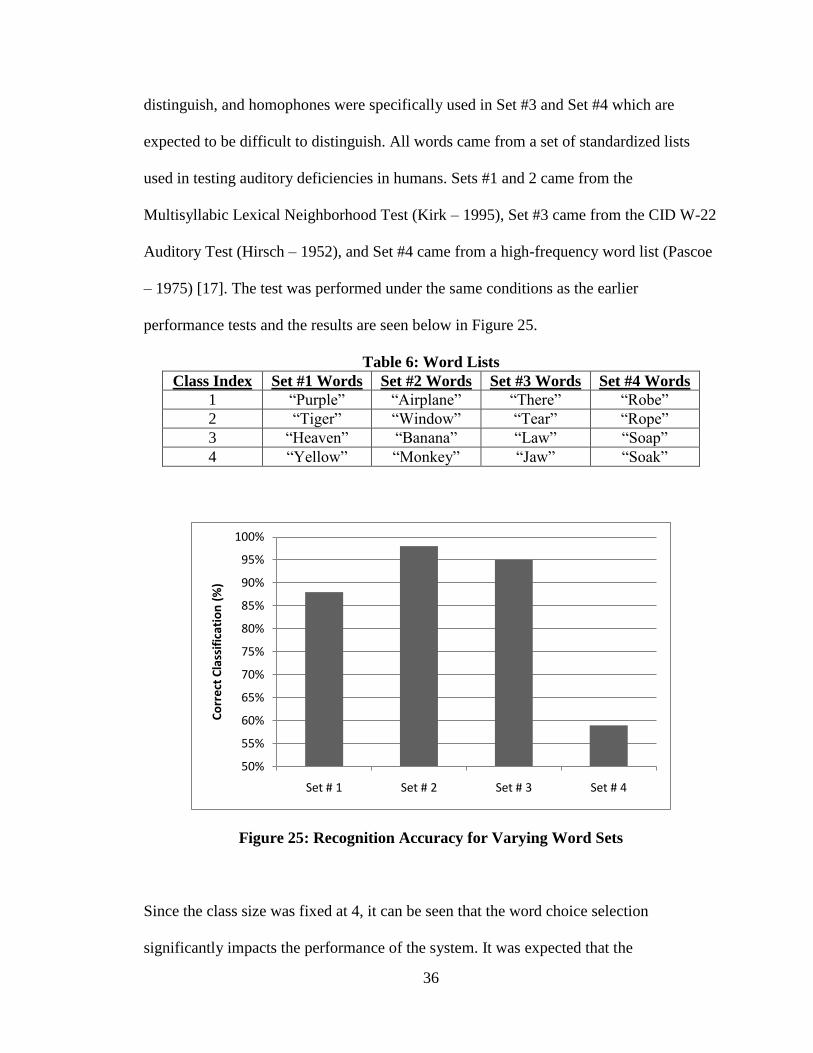
Table 6: Word Lists

Class Index Set #1 Words Set #2 Words Set #3 Words Set #4 Words

1 “Purple” “Airplane” “There” “Robe”

2 “Tiger” “Window” “Tear” “Rope”

3 “Heaven” “Banana” “Law” “Soap”

4 “Yellow” “Monkey” “Jaw” “Soak”

Figure 25: Recognition Accuracy for Varying Word Sets

Since the class size was fixed at 4, it can be seen that the word choice selection

significantly impacts the performance of the system. It was expected that the

50%

55%

60%

65%

70%

75%

80%

85%

90%

95%

100%

Set # 1 Set # 2 Set # 3 Set # 4

Co

rre

ct C

lass

ific

atio

n (

%)

37

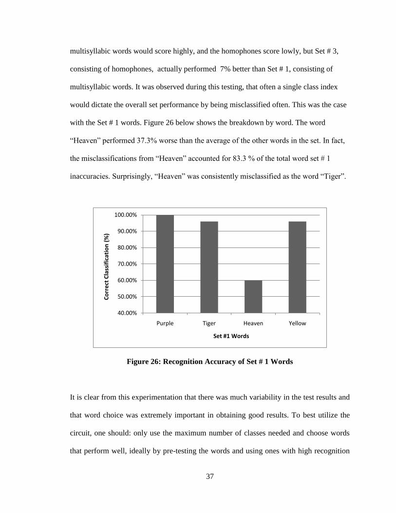
multisyllabic words would score highly, and the homophones score lowly, but Set # 3,

consisting of homophones, actually performed 7% better than Set # 1, consisting of

multisyllabic words. It was observed during this testing, that often a single class index

would dictate the overall set performance by being misclassified often. This was the case

with the Set # 1 words. Figure 26 below shows the breakdown by word. The word

“Heaven” performed 37.3% worse than the average of the other words in the set. In fact,

the misclassifications from “Heaven” accounted for 83.3 % of the total word set # 1

inaccuracies. Surprisingly, “Heaven” was consistently misclassified as the word “Tiger”.

Figure 26: Recognition Accuracy of Set # 1 Words

It is clear from this experimentation that there was much variability in the test results and

that word choice was extremely important in obtaining good results. To best utilize the

circuit, one should: only use the maximum number of classes needed and choose words

that perform well, ideally by pre-testing the words and using ones with high recognition

40.00%

50.00%

60.00%

70.00%

80.00%

90.00%

100.00%

Purple Tiger Heaven Yellow

Co

rre

ct C

lass

ific

atio

n (

%)

Set #1 Words

38

accuracy. As long as these two conditions are met, this particular circuit can perform with

very high recognition accuracy (correct classification >90% for 5 or fewer classes).

39

Conclusion

In conclusion, the three goals of the project were all completed successfully. A circuit

was constructed around the HM2007 IC creating a stand-alone hardware application of a

neural network system. After experimentation dissecting the most common speech

recognition neural network architectures, the architecture was determined to most closely

fit a time-delay neural network architecture, and the parameters were estimated. The

system performance was measured through various experiments and determined to

perform with a very high recognition accuracy for a small number of classes. The circuit

had recognition accuracy greater than 94.5% for 5 classes or fewer which would be

sufficient for many speech recognition applications.

40

References

[1] Minsky, M., Papert, S. (1969). “Perceptrons-Expanded Edition: An Introduction to

Computational Geometry”. MIT Press, Cambridge, MA

[2] Demuth, H., Beale, M., & Hagan, M. (2009). “Neural Network Toolbox 6 User’s

Guide”. Mathworks Inc., Natick, MA

[3] Hagan, T.M, Demuth, B.H., & Beale, H.M. (1996). “Neural Network Design”.

Campus Publishing Service, Colorado University Bookstore, University of Colorado at

Boulder

[4] Katagiri, S. (2000). “Handbook of Neural Networks for Speech Processing”. , Artech

House, Norwood, MA

[5] Rabiner, L., Juang, B. (1993). “Fundamentals of Speech Recognition”. Prentice-Hall,

Inc. Englewood Cliffs, NJ

[6] Voice Frequency [Internet]. Last updated March 7, 2009 [cited September 6, 2009].

Available from http://en.wikipedia.org/wiki/Voice_frequency

[7] Spectrogram [Internet]. Last updated August 1, 2009 [cited September 5, 2009].

Available from http://en.wikipedia.org/wiki/Spectrogram

[8] Specgram.m MATLAB help document. MATLAB version 7.0 (R14). Mathworks Inc.

Natick, MA

[9] Forsberg, M. (2003). “Why is Speech Recognition Difficult”. Chalmers University of

Technology.

[10] HM2007 Speech Recognition IC Datasheet. Hualon Microelectronics Corporation.

[11] SR-06/SR-07 Speech Recognition Kit. Images SI Inc. Staten Island, NY

[12] 74LS373 Datasheet (2002). Texas Instruments. Dallas, TX

41

[13] 4511 Datasheet (1995). Philips Semiconductors.

[14] Mammone, R. (1994). “Artificial Neural Networks for Speech and Vision”,

Chapman & Hall, London

[15] HM6264 Series Datasheet. Hitachi America Ltd. San Jose, CA

[16] Weinstein, C. (1990). “Opportunities for Advanced Speech Processing in Military

Computer-Based Systems”, MIT Lincoln Laboratory, Lexington, MA

[17] Gelfand, S. (2001). “Essentials of Audiology”. Thieme Medical Publishers, Inc.

New York, NY

[18] Anderson, C. and Setter, C. (1996). [Internet] “Talking Toaster – Final Report”

Available from http://www.the4cs.com/~corin/cse477/toaster/FinalReport.html

[19] Misir, A. et al. (2004). [Internet] “Voice Activated Robotic Arm” Available from

http://classes.cecs.ucf.edu/seecsseniordesign/fa2003sp2004/g16/SENIOR%20DESIGN%

20II/design_reviews.htm

[20] Demr, A. [Internet] “Speech Operated Electric Wheelchair” Available from

http://hackaday.com/2008/05/17/voice-controlled-wheel-chair/

[21] Zhang, E. (2002). [Internet] “Advanced Rescue Vision System” Available from

http://www.freepatentsonline.com/6476391.html

42

APPENDIX A

%% A Hardware Implementation of an Artificial Neural Network

% Created by Justin Wodarck - August 28,2009

% This code was used to determine the architecture and parameters of the

% HM2007 IC

%% Test Series # 1 - Testing for time-dependent architecture

% Test # 1 - Amplitude versus Time

[y,Fs]=wavread('neural network 4.wav');

y1=5.*y;

y2=flipud(y1);

% Plotting the waveforms

figure(1)

plot(y1,'k-')

hold on

plot(y2,'b--')

figure(2)

[Y1,n1]=pwelch(y1,[],[],[],Fs);

[Y2,n2]=pwelch(y2,[],[],[],Fs);

plot(n1,10*log10(Y1),'k-',n2,10*log10(Y2),'b--')

% Emitting the sound for testing the circuit

pause

player=audioplayer(y1,Fs);

play(player);

pause

player=audioplayer(y2,Fs);

play(player);

pause

clear

close all

% Test # 2 - Frequency versus Time

Ts=0.0001;

Fs=1/Ts;

x=0:Ts:1;

X1=0.25.*sin(2*pi*1000.*x);

X2=0.25.*sin(2*pi*2000.*x);

X_comp=X1.*(x<0.5)+X2.*(x>0.5);

X_comp2=X2.*(x<0.5)+X1.*(x>0.5);

% Plotting the waveforms

figure(1)

plot(X_comp,'k-')

hold on

plot(X_comp2,'b--')

43

figure(2)

[XX1,n1]=pwelch(X_comp,[],[],[],Fs);

[XX2,n2]=pwelch(X_comp2,[],[],[],Fs);

plot(n1,10*log10(XX1),'k-',n2,10*log10(XX2),'b--')

figure(3)

x=X_comp;

specgram(x,2^12,Fs,kaiser(500,5),475)

title('Spectrogram of X1-X2')

colormap bone

colorbar

figure(4)

x=X_comp2;

specgram(x,2^12,Fs,kaiser(500,5),475)

title('Spectrogram of X2-X1')

colormap bone

colorbar

% Emitting the sound for testing the circuit

pause

player=audioplayer(X_comp,Fs);

play(player);

pause

player=audioplayer(X_comp2,Fs);

play(player);

pause

clear

close all

%% Test Series # 2 - Determining TDNN Parameters

% Test # 1 - Delay Time

N=27;

Delta=1.92/(N+1);

Ts=0.0001;

Fs=1/Ts;

x=0:Ts:1;

q1=0.75.*sin(2*pi*500.*x);

q2=0.75.*sin(2*pi*550.*x);

q3=0.75.*sin(2*pi*(600).*x);

y3=q1.*(x<0.25)+q2.*(x>=0.25 & x<0.5)+q3.*(x>=0.5 & x<0.75)+q1.*(x>=0.75);

y4=q1.*(x<0.25+Delta)+q2.*(x>=(0.25+Delta)& x<0.5)+q3.*(x>=0.5 &

x<(0.75+Delta))+q1.*(x>=(0.75+Delta));

% Plotting the waveforms

figure(1)

x=y3;

specgram(x,2^12,Fs,kaiser(500,5),475)

title('Spectrogram of Y3')

colormap bone

44

colorbar

figure(2)

x=y4;

specgram(x,2^12,Fs,kaiser(500,5),475)

title('Spectrogram of Y4')

colormap bone

colorbar

% Emitting the sound for testing the circuit

pause

player=audioplayer(y3,Fs);

play(player);

pause

player=audioplayer(y4,Fs);

play(player);

pause

clear

close all

% Test # 2 - Upper and Lower Frequency Bounds

Freq=2000;

Ts=0.0001;

Fs=1/Ts;

x=0:Ts:1;

Bound=0.5.*sin(2*pi*Freq.*x);

% Emitting the sound for testing the circuit

pause

player=audioplayer(Bound,Fs);

play(player);

pause

clear

close all

% Test # 3 - Determining the Frequency Resolution

Res=(2000-400)/64;

Ts=0.0001;

Fs=1/Ts;

x=0:Ts:1;

z1=0.25.*sin(2*pi*1000.*x);

z2=0.25.*sin(2*pi*(1000+Res).*x);

z3=z1.*(x<0.5)+z2.*(x>0.5);

z4=z2.*(x<0.5)+z1.*(x>0.5);

% Emitting the sound for testing the circuit

pause

player=audioplayer(z3,Fs);

play(player);

pause

player=audioplayer(z4,Fs);

play(player);

45

pause

clear

close all

46

APPENDIX B

%% Voiceprint Figure Code

% Created by Justin Wodarck - September 9, 2009

% This code was used to create Figure 18 in the Final Report of my

% Master's Project "A Hardware Implementation of a Neural Network"

[y,Fs]=wavread('neural network 4.wav');

y=5.*y;

y2=y(1:11:end,1);

y2=y2(2928:end,1);

[B,f,t]=specgram(y2,80,Fs/11);

t=t(4:7:end);

B=abs(B);

for j=1:41

for i=1:round(length(B)/7)

B_new(j,i)=mean(B(j,((1+(7*(i-1))):(7+(7*(i-1)))))')';

end

end

Q=(max(max(B_new))-min(min(B_new)))/257;

A=min(min(B_new)):Q:max(max(B_new));

B_newR=reshape(B_new,41*27,1);

New=quantalph(B_newR,A);

B_newR2=reshape(New,41,27);

imagesc(t,f'',B_newR2)

axis xy

title('Neural Network Voiceprint')

colormap bone

colorbar

axis([0 1.85 400 2000])

xlabel('Time (seconds)')

ylabel('Frequency (Hz)')