REDUCED�ORDER AERODYNAMIC MODELS FOR

AEROELASTIC CONTROL OF TURBOMACHINES

by

KAREN ELIZABETH WILLCOX

B�E� University of Auckland� New Zealand ������S�M� Massachusetts Institute of Technology �����

SUBMITTED TO THE DEPARTMENT OF AERONAUTICS ANDASTRONAUTICS

IN PARTIAL FULFILLMENT OF THE REQUIREMENTS FOR THE DEGREEOF

DOCTOR OF PHILOSOPHY

at the

MASSACHUSETTS INSTITUTE OF TECHNOLOGY

February ���

c� Massachusetts Institute of Technology ���� All rights reserved�

AuthorDepartment of Aeronautics and Astronautics

November �� ����

Certi�ed byJaime Peraire

Professor of Aeronautics and Astronautics

Certi�ed byJames Paduano

Principal Research Engineer� Department of Aeronautics and Astronautics

Certi�ed byMark Drela

Associate Professor of Aeronautics and Astronautics

Certi�ed byJacob White

Professor of Electrical Engineering and Computer Science

Accepted byAssociate Professor Nesbitt Hagood

Chairman� Department Graduate Committee

Reduced�Order Aerodynamic Models for Aeroelastic Control of

Turbomachines

by

Karen Elizabeth Willcox

Submitted to the Department of Aeronautics and Astronauticson November �� ����� in partial ful�llment of the

requirements for the degree ofDoctor of Philosophy

Abstract

Aeroelasticity is a critical consideration in the design of gas turbine engines� both for stability andforced response� Current aeroelastic models cannot provide high��delity aerodynamics in a formsuitable for design or control applications� In this thesis low�order� high��delity aerodynamic modelsare developed using systematic model order reduction from computational �uid dynamic CFDmethods� Reduction techniques are presented which use the proper orthogonal decomposition� andalso a new approach for turbomachinery which is based on computing Arnoldi vectors� This methodmatches the input�output characteristic of the CFD model and includes the proper orthogonaldecomposition as a special case� Here� reduction is applied to the linearised two�dimensional Eulerequations� although the methodology applies to any linearised CFD model� Both methods makee�cient use of linearity to compute the reduced�order basis on a single blade passage�

The reduced�order models themselves are developed in the time domain for the full blade row and castin state�space form� This makes the model appropriate for control applications and also facilitatescoupling to other engine components� Moreover� because the full blade row is considered� the modelscan be applied to problems which lack cyclic symmetry� Although most aeroelastic analyses assumeeach blade to be identical� in practice variations in blade shape and structural properties exist dueto manufacturing limitations and engine wear� These blade to blade variations� known as mistuning�have been shown to have a signi�cant e ect on compressor aeroelastic properties�

A reduced�order aerodynamic model is developed for a twenty�blade transonic rotor operating inunsteady plunging motion� and coupled to a simple typical section structural model� Stability andforced response of the rotor to an inlet �ow disturbance are computed and compared to resultsobtained using a constant coe�cient model similar to those currently used in practice� Mistuningof this rotor and its e ect on aeroelastic response is also considered� The simple models are foundto inaccurately predict important aeroelastic results� while the relevant dynamics can be accuratelycaptured by the reduced�order models with less than two hundred aerodynamic states� Modelsare also developed for a low�speed compressor stage in a stator�rotor con�guration� The stator isshown to have a signi�cant destabilising e ect on the aeroelastic system� and the results suggestthat analysis of the rotor as an isolated blade row may provide inaccurate predictions�

Thesis Supervisor� Jaime PeraireTitle� Professor of Aeronautics and Astronautics

Thesis Supervisor� James PaduanoTitle� Principal Research Engineer� Department of Aeronautics and Astronautics

�

Acknowledgments

So many people have contributed so much to this thesis� it is di�cult to know where to begin�

My advisor� Prof� Jaime Peraire� has contributed to making my time at MIT very enjoyable by

providing me with an outstanding balance of academic support and freedom� I am extremely lucky

to have not only had the bene�t of excellent research advice� but also the freedom to pursue my extra�

curricular activities� My second advisor� Dr� Jim Paduano� has also provided me with invaluable

help and practical suggestions� I especially thank him for the opportunities he has provided for

interesting applications of my research and interaction with industry� I have been lucky enough

to have a large and very diverse committee� Thanks to Prof� Mark Drela for always knowing the

right answer� and o ering valuable insight to problems� to Prof� Jacob White for introducing me to

the Arnoldi method� and the most interesting result of my thesis� to my minor advisor Prof Carlos

Cesnik� and to Dr� Choon Tan for teaching me what I know about internal �ows� I would also like

to thank Prof� Ken Hall who had many helpful suggestions for my eigenmode problems while he

was here at MIT� and Ben Shapiro for the joint work on mistuning and allowing me to use MAST�

Thanks to the current FDRL crew� who are all probably glad they don�t have to hear my presentation

again� Especially I would like to thank Ed and Anjie� whom I have plagued with countless questions

on LaTex� Unix and every other aspect of my computer problems� Thanks also to Prof� Dave

Darmofal for reading my thesis and o ering me a great deal of important and relevant feedback�

and to Tolu �the Unix master� for shell scripts which saved my life and a wonderful program called

Cplot although I still want my money refunded� Thanks also to Bob Haimes who provides a unique

and honest perspective on life at MIT� and has provided me with much encouragement� I would

especially like to thank Jean Sofronas whose hard work so often goes unnoticed� The organisation

she has brought to the lab has made life so much easier� especially for those of us trying to track

down Jaime�

To those who have gone before and escaped � my former o�ce mate �by the way my real name is

Josh Elliot� for setting the example of thesis defense preparation by the way � London is further

than Florida� Josh and for providing the inspiration for the infamous Mardi Gras trip� To the

incorrigible group who helped me survive my �rst years at MIT � Graeme� Ray� Jim� Guy� Mike�

Carmen� Lou and Ernie� In particular� to Graeme Shaw who has been like a brother to me� to Mike

Fife for being the wonderfully unique person that he is� and to Ray for staying behind to share the

�later years��

Away from the lab� I have been fortunate to meet many interesting people and form some priceless

�

friendships� I would like to thank my housemates Matt and Chris for many fun times� and for not

throwing out the vegemite� Pat Kreidl who always gave me the best perspective on things when I

needed it most� and showed us all not to be afraid of following our dreams� Rebecca Morss who

has been adventurous or stupid enough to go with some of my crazier ideas and out�ts� Blotto

Van Der Helm for some of my more exciting moments in a car� Simon Karecki for introducing me

to Jagermeister� Matthew Dyer for introducing me to bridge� Samuel Mertens for all the chocolate�

and Yoshi Uchida for many great hours of chocolate� ice�cream and conversation� I would also like

to thank Tienie Van Schoor for running the most hospitable company ever� Brett Masters for being

the other NZer� and Gert Gogga Muller for his help in my endeavours to master Afrikaans�

I would especially like to thank William Web Ellis � without that crazy game I would never have

survived graduate school� In particular� my years playing with the MIT women�s rugby team are

some of the best sporting memories of my life � too many great ruggers to mention here� and great

coaches� I just hope I was not too bossy on the �eld� Playing with Beantown RFC has provided

me with a fantastic sporting challenge� and also the opportunity to meet many inspiring women�

In particular I would like to thank Sonya Church� Liz Satter�eld� Jen Crouse� Anna Mackay and

Daniel Scary Spice for their friendship� I would have liked to thank the All Blacks for providing me

with the best post�defense celebration opportunity� but ���� Rugby has given me the opportunity to

form some very special friendships � in particular with Marianne Bitler who taught me all I know

about midri shirts � I�m just sorry I never learned to go without sleep� and Judi Burgess for the

margaritas when I needed them and when I really didn�t� and for really appreciating the little brown

bird in me�

I must also thank the faculty and students of my undergrad department at the University of Auckland

for the encouragement and help to come to the US for grad school� In particular� Dr Roger Nokes

provided some much needed support during the GREs and application process� To my friends James

Deaker� Mike O�Sullivan� JP Hansen and Tim Watson � thanks for the visits and the emails to this

poor stranded kiwi� And of course thanks to Ivan Brunton and Chris Bradley for their best e orts

to sabotage my defense preparation� and to Mark and Justine Sagar for the wonderful times while

they were in Boston and the coolest bathroom ever��

I owe a special debt of gratitude to my Thursday afternoon counselling group for their unique

perspective on life� I am honoured to have developed a friendship with Michael Cook� who is one

of the most unsel�sh people I have ever met� I would also like to give special thanks to Tony and

Doreen Puttick who have been my �American� surrogate parents and have contributed so much to

my life here in Boston� I only hope I can one day repay your hospitality down under�

�

I specially owe thanks to my sole�mate Vanessa Chan for recognising my accent� never being the

voice of reason� and always providing the transport� Who would have thought MIT could be so

much fun� And last but certainly not least� Jaco Pretorius who has shared so much of the pain� and

now hopefully the rewards and a more peaceful night�s sleep� He has provided me with all the

support and understanding to �nish this degree� and I have the best beer cooler in the world� Beste

wense met jou beroep as professionele� sosiale gholfer �

Finally� I must thank my family� who from afar have provided so much love and support� To Mum�

Dad� Dawn and Keith � thanks for the emails� the letters� the newspaper clippings� the lamb� the

vegemite and the clothes to let me dress like a real kiwi� I will thank in advance my brother for the

ride in the F���� and my sister for the visit to her excavation site� and wish them both the best of

luck in their careers�

And �nally to my grandmothers� Grace and Flora� two very unique and inspiring women who over

the last �� years have done so much for me� To you both I dedicate this thesis� Happy reading�

�

Contents

List of Figures �

� Introduction ��

��� Aeroelastic Modelling � � � � � � � � � � � � � � � � � � � � � � � � � � � � � � � � � � � ��

��� Model Order Reduction � � � � � � � � � � � � � � � � � � � � � � � � � � � � � � � � � � ��

��� Reduced�Order Modelling Applications � � � � � � � � � � � � � � � � � � � � � � � � � � ��

��� Outline � � � � � � � � � � � � � � � � � � � � � � � � � � � � � � � � � � � � � � � � � � � ��

� Aeroelastic Model ��

��� Aerodynamic Model � � � � � � � � � � � � � � � � � � � � � � � � � � � � � � � � � � � � ��

����� Governing Equations � � � � � � � � � � � � � � � � � � � � � � � � � � � � � � � � ��

����� Nonlinear Model � � � � � � � � � � � � � � � � � � � � � � � � � � � � � � � � � � ��

����� Linearised Model � � � � � � � � � � � � � � � � � � � � � � � � � � � � � � � � � � ��

����� Linearised Boundary Conditions � � � � � � � � � � � � � � � � � � � � � � � � � ��

����� Modal Analysis � � � � � � � � � � � � � � � � � � � � � � � � � � � � � � � � � � � ��

��� CFD Model Validation � � � � � � � � � � � � � � � � � � � � � � � � � � � � � � � � � � � ��

����� UTRC Low�Speed Cascade � � � � � � � � � � � � � � � � � � � � � � � � � � � � ��

����� DFVLR Transonic Cascade � � � � � � � � � � � � � � � � � � � � � � � � � � � � ��

����� First Standard Con�guration � � � � � � � � � � � � � � � � � � � � � � � � � � � ��

�

��� Structural Model � � � � � � � � � � � � � � � � � � � � � � � � � � � � � � � � � � � � � � ��

��� Coupled Aerodynamic�Structural Model � � � � � � � � � � � � � � � � � � � � � � � � � ��

� Reduced�Order Aerodynamic Modelling �

��� Aerodynamic In�uence Coe�cients � � � � � � � � � � � � � � � � � � � � � � � � � � � � ��

��� Reduction Using Congruence Transforms � � � � � � � � � � � � � � � � � � � � � � � � � ��

��� Eigenmode Representation � � � � � � � � � � � � � � � � � � � � � � � � � � � � � � � � � ��

��� Proper Orthogonal Decomposition � � � � � � � � � � � � � � � � � � � � � � � � � � � � ��

����� Snapshot Generation � � � � � � � � � � � � � � � � � � � � � � � � � � � � � � � � ��

��� Arnoldi�Based Model Order Reduction � � � � � � � � � � � � � � � � � � � � � � � � � � ��

����� Computation of Arnoldi Basis � � � � � � � � � � � � � � � � � � � � � � � � � � � ��

����� Arnoldi Approach versus POD � � � � � � � � � � � � � � � � � � � � � � � � � � ��

����� Arnoldi Model Extensions � � � � � � � � � � � � � � � � � � � � � � � � � � � � � ��

��� Projection onto Optimal Basis Vectors � � � � � � � � � � � � � � � � � � � � � � � � � � ��

����� Static Corrections � � � � � � � � � � � � � � � � � � � � � � � � � � � � � � � � � ��

����� Reduced�Order Models � � � � � � � � � � � � � � � � � � � � � � � � � � � � � � � ��

��� Reduced�Order Modelling Summary � � � � � � � � � � � � � � � � � � � � � � � � � � � ��

� Reduced�Order Modelling of a Transonic Rotor �

��� Aerodynamic Reduced�Order Models � � � � � � � � � � � � � � � � � � � � � � � � � � � ��

����� POD Reduced�Order Model � � � � � � � � � � � � � � � � � � � � � � � � � � � � ��

����� Arnoldi Reduced�Order Model � � � � � � � � � � � � � � � � � � � � � � � � � � ��

��� Aerodynamic Forced Response � � � � � � � � � � � � � � � � � � � � � � � � � � � � � � ��

��� Coupled Aerodynamic�Structural Reduced�Order Model � � � � � � � � � � � � � � � � ��

��� Comparison of POD with In�uence Coe�cient Model � � � � � � � � � � � � � � � � � ��

��� Physical Mode Identi�cation � � � � � � � � � � � � � � � � � � � � � � � � � � � � � � � � ��

�

� Mistuning �

��� Mistuning Analysis via Symmetry Considerations � � � � � � � � � � � � � � � � � � � � ��

��� Reduced�Order Models for Mistuning Analysis � � � � � � � � � � � � � � � � � � � � � ���

��� Mistuning Analysis of Transonic Rotor � � � � � � � � � � � � � � � � � � � � � � � � � � ���

����� Reduced�Order Aerodynamic Model � � � � � � � � � � � � � � � � � � � � � � � ���

����� Aerodynamic In�uence Coe�cient Model � � � � � � � � � � � � � � � � � � � � ���

��� Mistuning Summary � � � � � � � � � � � � � � � � � � � � � � � � � � � � � � � � � � � � ���

Multiple Blade Row Analysis ��

��� Blade Row Coupling � � � � � � � � � � � � � � � � � � � � � � � � � � � � � � � � � � � � ���

��� GE Low Speed Compressor � � � � � � � � � � � � � � � � � � � � � � � � � � � � � � � � ���

����� Steady�State Solutions � � � � � � � � � � � � � � � � � � � � � � � � � � � � � � � ���

����� Unsteady Analysis � � � � � � � � � � � � � � � � � � � � � � � � � � � � � � � � � ���

��� Summary � � � � � � � � � � � � � � � � � � � � � � � � � � � � � � � � � � � � � � � � � � ���

Conclusions and Recommendations ���

A GMRES Algorithm ��

Bibliography ���

�

List of Figures

��� Concept of reduced�order modelling from CFD� Unsteady inputs include blade mo�

tion and incoming �ow disturbances� Outputs of interest are typically outgoing �ow

disturbances and blade forces and moments� � � � � � � � � � � � � � � � � � � � � � � � ��

��� Input�output view of aeroelastic model� � � � � � � � � � � � � � � � � � � � � � � � � � ��

��� Rectilinear� two�dimensional representation of compressor stage� � � � � � � � � � � � ��

��� Computational domain for single blade row� Inlet boundary �� exit boundary ��

blade surfaces � and periodic boundaries �� � � � � � � � � � � � � � � � � � � � � � ��

��� Control volume Vj associated to a generic node j of an unstructured grid a Interior

node� b Boundary node� � � � � � � � � � � � � � � � � � � � � � � � � � � � � � � � � � ��

��� Computational domain for solution of steady�state �ow� Boundary conditions are

applied at blade surfaces and passage inlet and exit� Periodic conditions are applied

at dashed boundaries� Inlet and exit boundary conditions shown assume subsonic

axial �ow� � � � � � � � � � � � � � � � � � � � � � � � � � � � � � � � � � � � � � � � � � � ��

��� CFD grid for UTRC subsonic blade� ���� points� ���� triangles� � � � � � � � � � � � ��

��� Pressure distribution for UTRC subsonic blade� experimental data points and CFD

results lines� M � ������ � � ���� � � � � � � � � � � � � � � � � � � � � � � � � � � ��

��� CFD grid for DFVLR transonic rotor� ���� points� ���� triangles� � � � � � � � � � � ��

��� Steady�state pressure contours for DFVLR transonic rotor� M � ����� � � ������ � ��

���� Pressure distribution for DFVLR transonic blade� experimental data points and

CFD results lines� M � ����� � � ������ � � � � � � � � � � � � � � � � � � � � � � ��

�

���� First standard con�guration blade pressure distribution� M � ����� � � ����� � � ���� ��

���� First standard con�guration� torsional aerodynamic damping coe�cient as a function

of interblade phase angle� M � ����� � � ����� k � ������ � � � � � � � � � � � � � � � ��

���� Typical section structural model for blade i� � � � � � � � � � � � � � � � � � � � � � � � ��

��� Eigenvalue spectrum for small problem� n � ���� Eigenvalues for unperturbed

matrix diamonds and random perturbations of order ���� squares and ������

plus signs of the diagonal� � � � � � � � � � � � � � � � � � � � � � � � � � � � � � � � � ��

��� Eigenvalue spectrum for large problem� n � ����� Eigenvalues for unperturbed

matrix plus signs and random perturbations of order ������ diamonds of the

diagonal� � � � � � � � � � � � � � � � � � � � � � � � � � � � � � � � � � � � � � � � � � � � ��

��� Computational domain for two passages of the DFVLR transonic rotor� ���� nodes�

���� triangles per blade passage� � � � � � � � � � � � � � � � � � � � � � � � � � � � � � ��

��� POD Eigenvalue spectra for transonic cascade in plunge� M � ����� � � ��� ����� � ��

��� Eigenvalue spectrum for POD reduced�order aerodynamic system� Six modes per

interblade phase angle total ��� modes� � � � � � � � � � � � � � � � � � � � � � � � � ��

��� Eigenvalue spectrum for Arnoldi reduced order aerodynamic system� Six modes per

interblade phase angle total ��� modes� All basis vectors computed about s � �� � ��

��� Pulse input in plunge� g � ����� � � � � � � � � � � � � � � � � � � � � � � � � � � � � � � ��

��� Pulse response for POD reduced�order model and linearised simulation code� � � ���

g � ����� M � ����� � � � � � � � � � � � � � � � � � � � � � � � � � � � � � � � � � � � � ��

��� Pulse response for Arnoldi reduced�order model and linearised simulation code� � �

��� g � ����� M � ����� � � � � � � � � � � � � � � � � � � � � � � � � � � � � � � � � � � ��

��� Pulse response for Arnoldi reduced�order model with �� modes� POD reduced�order

model with � modes and linearised simulation code� � � ��� g � ���� M � ����� � � � ��

��� Pulse displacement input dashed line and blade lift force response solid line for

Arnoldi reduced�order model� Six modes for � � �� and ten modes for all other

interblade phase angles total ��� modes� g � ����� M � ����� � � � � � � � � � � � � ��

��

���� Eigenvalue spectrum for Arnoldi reduced�order model� Purely aerodynamic eigenval�

ues diamonds and coupled aerodynamic�structural system plus signs� ��� aero�

dynamic states� �� structural states� M � ����� � � ���� k � ����� � �� � � � � � � � ��

���� Zoom of structural eigenvalues� Eigenvalues are numbered by nodal diameter� M � �����

� � ���� k � ����� � �� � � � � � � � � � � � � � � � � � � � � � � � � � � � � � � � � � � ��

���� Aerodynamic work per cycle as a function of interblade phase angle and reduced

frequency for transonic rotor� � � � � � � � � � � � � � � � � � � � � � � � � � � � � � � � ��

���� Aerodynamic work per cycle as a function of interblade phase angle for reduced fre�

quencies of k � ����� ����� ����� � � � � � � � � � � � � � � � � � � � � � � � � � � � � � � ��

���� Coupled system response to an initial plunge displacement input at blade � � blade

displacement dashed line and blade vertical force solid line� � � ���� k �

����� � �� � � � � � � � � � � � � � � � � � � � � � � � � � � � � � � � � � � � � � � � � � ��

���� Eigenvalues for POD reduced�order model� Purely aerodynamic eigenvalues dia�

monds and coupled aerodynamic�structural system plus signs� �� aerodynamic

states� �� structural states� � � ���� k � ����� � �� � � � � � � � � � � � � � � � � � � ��

���� Structural eigenvalues for reduced�order model and aerodynamic in�uence coe�cient

model evaluated at c � n � ���� Also shown is the � � �� eigenvalue for in�uence

coe�cients evaluated at � ����� Structural parameters � � � ���� k � ����� � ��

Eigenvalues are numbered by their nodal diameter� � � � � � � � � � � � � � � � � � � � ��

���� Damping and frequency of structural modes for reduced�order model and in�uence

coe�cient models at c � ��� and c � ����� � � ���� k � ����� � �� � � � � � � � ��

���� Blade force response amplitude to imposed sinusoidal motion� Reduced�order model

prediction solid lines� in�uence coe�cient model prediction dotted lines and CFD

solution crosses� plus signs and diamonds� From the top � � � ���� � � ���� and

� � ����� � � � � � � � � � � � � � � � � � � � � � � � � � � � � � � � � � � � � � � � � � � ��

���� Blade displacement response amplitude to a sinusoidal axial velocity disturbance at

the passage inlet� � � ����� � � � � � � � � � � � � � � � � � � � � � � � � � � � � � � � � ��

���� Blade force response amplitude to a sinusoidal axial velocity disturbance at the pas�

sage inlet� � � ����� � � � � � � � � � � � � � � � � � � � � � � � � � � � � � � � � � � � � ��

��

���� Parabolically distributed eigenvalues for Arnoldi reduced order aerodynamic system

with ��� aerodynamic states total� � � � � � � � � � � � � � � � � � � � � � � � � � � � � ��

���� Perturbation vorticity contours for a �ow solution at t � � constructed from eigen�

mode with � � ����� � ����i� � � � � � � � � � � � � � � � � � � � � � � � � � � � � � � � ��

���� Perturbation velocity vectors for a �ow solution at t � � constructed from eigenmode

with � � ����� � ����i� � � � � � � � � � � � � � � � � � � � � � � � � � � � � � � � � � � ��

���� Perturbation velocity vectors for a �ow solution at t � �� constructed from eigen�

mode with � � ����� � ����i� � � � � � � � � � � � � � � � � � � � � � � � � � � � � � � � ��

��� Tuned structural eigenvalues for reduced�order model� k � ������ � � ���� �

�������� Eigenvalues are numbered by their nodal diameter� � � � � � � � � � � � � � ���

��� Random mistuning of DFVLR rotor� Top� random mistuning pattern� Bottom�

tuned eigenvalues diamonds� mistuned eigenvalues plus signs� � � � � � � � � � � � ���

��� Random mistuning of DFVLR rotor� Forced response of tuned system solid line

and mistuned system dotted lines to an inlet disturbance in the ninth spatial mode� ���

��� Optimal mistuning of DFVLR rotor� Top� optimal mistuning pattern� Bottom� tuned

eigenvalues diamonds� mistuned eigenvalues plus signs� � � � � � � � � � � � � � � � ���

��� Optimal plus random mistuning of DFVLR rotor� Top� optimal plus random mis�

tuning pattern� Bottom� tuned eigenvalues diamonds� mistuned eigenvalues plus

signs� � � � � � � � � � � � � � � � � � � � � � � � � � � � � � � � � � � � � � � � � � � � � ���

��� Optimal plus random mistuning of DFVLR rotor� Forced response of tuned system

solid line and mistuned system dotted lines to an inlet disturbance in the ninth

spatial mode� � � � � � � � � � � � � � � � � � � � � � � � � � � � � � � � � � � � � � � � � ���

��� Random mistuning of DFVLR transonic rotor� Top� reduced�order model eigenvalues�

tuned diamonds and mistuned plus signs� Bottom� in�uence coe�cient model

eigenvalues� tuned diamonds and mistuned plus signs� � � � � � � � � � � � � � � � ���

��� Random mistuning of DFVLR transonic rotor� Top� tuned eigenvalues� reduced�order

model diamonds and in�uence coe�cient model plus signs� Bottom� mistuned

eigenvalues� reduced�order model diamonds and in�uence coe�cient model plus

signs� � � � � � � � � � � � � � � � � � � � � � � � � � � � � � � � � � � � � � � � � � � � � ���

��

��� Random mistuning of DFVLR transonic rotor� Forced response to inlet disturbance in

the � � � mode for reduced�order model left and in�uence coe�cient model right�

Solid line denotes the tuned response� dotted lines are the mistuned response� � � � � ���

���� Random mistuning of DFVLR transonic rotor� Forced response to inlet disturbance

in the � � �� mode for reduced�order model left and in�uence coe�cient model

right� Solid line denotes the tuned response� dotted lines are the mistuned response� ���

��� Instantaneous con�guration of rotor and stator� Grid point j is in the rotor inlet

plane� while points k and k � � are in the stator exit plane� � � � � � � � � � � � � � � ���

��� Stator and rotor geometry for a single stage of the GE low�speed compressor� � � � � ���

��� Velocity triangles for third stage of GE low�speed compressor� Relative Mach numbers

for rotor� absolute Mach numbers for stator� � � � � � � � � � � � � � � � � � � � � � � � ���

��� Mach contours for GE low�speed compressor� third stage rotor� M � ������ � � ���������

��� Mach contours for GE low�speed compressor� third stage stator� M � ������ � � ���������

��� Aerodynamic eigenvalues for reduced�order models � rotor alone crosses� ��� states�

stator alone plus signs� ��� states and coupled system diamonds� ��� states� � � � ���

��� Zoom of aerodynamic eigenvalues for rotor and stator reduced�order models� � � � � ���

��� Aerodynamic response to pulse displacement input at blade �� Blade plunge dis�

placement prescribed� dotted line� rotor alone blade vertical force dashed line and

rotor�stator system blade vertical force solid line� � � � � � � � � � � � � � � � � � � � ���

��� Aerodynamic response of blade � to pulse displacement input at blade �� Rotor�alone

model dashed line and rotor�stator coupled model solid line� � � � � � � � � � � � � ���

���� Structural eigenvalues � rotor�alone system crosses and periodic loci for coupled sta�

tor�rotor model dots� Eigenvalues are numbered by their nodal diameter �� � � �����

� � ���� k � ���� � ����� � � � � � � � � � � � � � � � � � � � � � � � � � � � � � � ���

���� Periodic locus of structural eigenvalue for � � �� mode� � � � � � � � � � � � � � � � � ���

���� Response due to an initial plunge displacement at blade �� Blade displacement cal�

culated with rotor�alone model dashed lines and coupled stator�rotor model solid

lines� � � ���� k � ���� � ����� � � � � � � � � � � � � � � � � � � � � � � � � � � ���

��

���� Response due to an initial plunge displacement at blade �� Blade force calculated

with rotor�alone model dashed lines and coupled stator�rotor model solid lines�

� � ���� k � ���� � ����� � � � � � � � � � � � � � � � � � � � � � � � � � � � � � � ���

���� Response due to an initial plunge displacement at blade �� Displacement and force

on the thirteenth blade calculated with rotor�alone model dashed lines and coupled

stator�rotor model solid lines� � � ���� k � ���� � ����� � � � � � � � � � � � � ���

��

Chapter �

Introduction

Aeroelasticity is de�ned in �� as phenomena which exhibit appreciable reciprocal interaction �static

or dynamic� between aerodynamic forces and the deformations induced thereby in the structure of

a �ying vehicle� its control mechanisms� or its propulsion system� With the current trend towards

increased operating speeds and more �exible blading� aeroelasticity has become a critical consider�

ation in the design of gas turbine engines� and has a large impact on both stability and dynamic

response considerations�

Flutter is of particular concern in the design of bladed disks� Unstable vibrations may arise due

to coupling between the aerodynamics and the structural dynamics� If the �uid does work on a

vibrating blade so as to amplify or maintain the vibration� then the blade is said to be undergoing

�utter ��� � The ability to understand and predict this phenomenon is crucial to ensuring that the

engine component will operate within stability boundaries� and thus has a large impact on the design

process� Appropriate blade design� together with strategies for controlling the onset of instabilities�

can signi�cantly impact the stable operating range� potentially leading to better engine performance�

Dynamic response of the blades to various inputs� such as gusts or upstream obstacles� is an impor�

tant factor in determining the stress loads on the blades and the wear of the engine� In particular�

periodic forcing inputs� such as that due to an upstream structural support or blade row� may in�

duce a large blade response if the frequency of excitation is near the blade natural frequency� Blade

forced response vibrations can lead to high cycle fatigue� which can in turn cause blade failure�

Accurate prediction of blade response to external inputs can facilitate improved understanding of

forced response phenomena� allowing design strategies to be adopted to minimise their impact and

potentially prolong engine lifetimes�

��

��� Aeroelastic Modelling

Aeroelastic phenomena involve a complicated interaction between the aerodynamics and the struc�

tural dynamics of the blades� The challenge is to develop a model which accurately captures the

relevant dynamics of both the �uid and the structure� and more importantly� the interactions between

the two� Consideration of aeroelastic e ects is vital at the design stage to ensure that the compressor

will operate within an acceptable response region� The models must therefore satisfy an additional

requirement that they are computationally e�cient and thus practical to implement within a design

framework� Moreover� since aeroelastic instabilities represent a signi�cant impediment to obtaining

better engine performance� it may be desirable to consider active control strategies as a means of

extending the stable operating range� For such an approach to be possible� the aeroelastic model

must be suitable for incorporation to a control framework� which places restrictions upon the size

and form of the model�

Traditionally� the structural portion of the problem has been the easier of the two� since linear

models are generally adequate to model the structural dynamics� The disks are often assumed to

possess cyclic symmetry so that a model of just a single blade passage can be used to obtain the

dynamic response of the entire bladed disk� These dynamics can be accurately captured with a

�nite element model� The system of equations governing the structural dynamics is symmetric� so

that evaluation of natural modes eigenmodes is relatively straightforward� If deformation of blade

shapes is not considered to be important� a simpler structural model may be used� For example�

each blade might be given the freedom to move rigidly in certain displacement directions as in a

typical section model ��� � In this case� the number of structural states is greatly reduced�

For a given bladed disk geometry� the structural modes must be computed just once� and so it

is practical to perform a large �nite element analysis to obtain the modal information� However

the �ow must be modelled over a large range of operating conditions and forcing inputs� therefore

it is crucial that the aerodynamic model be computationally e�cient� Moreover� the system of

equations governing the aerodynamics are not symmetric� and it is very di�cult to determine the

�ow eigenmodes� We therefore require either an alternative means to determine the modes of a

complicated aerodynamic model� or a simpli�ed model which can be incorporated to the aeroelastic

analysis in its entirety� Such a model should be applicable over a wide range of geometries and

operating conditions� and also for a variety of excitation modes�

The most general aerodynamic model describes the blade forces as a function of blade motion� �ow

operating conditions� reduced frequency� blade geometry and a host of other problem parameters �� �

��

Within the state�of�the�art� the best possible aerodynamic models are obtained via computational

�uid dynamics CFD models� By numerically solving the unsteady Euler or Navier�Stokes equa�

tions� improved modelling of the �ow and better understanding of �uid phenomena can be obtained�

However these techniques are generally too computationally expensive to use for unsteady analyses�

especially if the full rotor and more than one blade row need to be considered� More e�cient meth�

ods for time�varying �ow can be obtained if the disturbances are small� and the unsteady solution

can be considered to be a small perturbation about a steady�state �ow ��� � In this case� a set of

linearised equations is obtained which can be time�marched to obtain the �ow solution at each in�

stant� Cyclic symmetry of the bladed disk can be used to decompose the linear problem into a series

of modal problems each containing a single spatial frequency� The analysis can then be carried out

for each mode on a single blade passage� Any of the CFD techniques result in models with tens of

thousands of states per blade passage� even in two dimensions� A model of this size is not practical

for computing stability boundaries� nor is it appropriate as a design tool� In addition� the number

of states is prohibitively high for control applications�

Instead� for aeroelastic analyses of turbomachines� the approach has typically been to use simpli�ed

aerodynamic models which can be incorporated into the aeroelastic framework in their entirety�

The �ow is usually assumed to be two�dimensional and potential� E�cient semi�analytic models

for lightly loaded thin blades have been developed for subsonic �ow ��� and for supersonic �ow �� �

These methods are useful near design conditions but inadequately predict the �ow o �design� as

blade loading e ects become important ��� and also do not exist for all �ow regimes� in particular

the modelling of transonic �ows poses a di�culty� Often� the assumptions involved in deriving

these simpli�ed models further restrict their range of validity� for instance they may not be valid

for high spatial frequency disturbances ��� � Another option is to use an �assumed�frequency�

method in which an aerodynamic model is derived from a CFD model for a speci�c case� The �ow

is assumed to be sinusoidal in time at a particular frequency� which allows high��delity in�uence

coe�cients to be calculated from the CFD model� Results have been reported using coe�cients

calculated from Whitehead�s incompressible� two�dimensional aerodynamic model ��� by Dugundji

and Bundas ��� � Crawley �� and Crawley and Hall �� use coe�cients for supersonic �ow calculated

from the model of Adamczyk and Goldstein �� � These in�uence coe�cients� although strictly only

valid at the temporal frequency selected usually the blade natural frequency� are then used to

provide the aerodynamic model for all �ows� They are coupled to the structural model as constant

coe�cients that are independent of problem parameters such as forcing frequency and boundary

conditions� If there is not a signi�cant degree of aerodynamic coupling in the system� then the

structural eigenvalues fall close to the blade natural frequency and the assumed�frequency model

��

predicts the aeroelastic system dynamics well� However� if there is a signi�cant amount of frequency

scatter or a large amount of aerodynamic damping� the assumed�frequency models do not provide

an accurate representation of the system dynamics� Moreover� even if the aeroelastic eigenvalues

are predicted accurately� these models can only predict the system forced response accurately if the

forcing frequency is close to the assumed frequency�

��� Model Order Reduction

Ideally� we would like to develop an aeroelastic model with a low number of states� but which

captures the system dynamics accurately over a range of frequencies and forcing inputs� This can

be achieved via reduced�order modelling in which a high�order� high��delity CFD model is projected

onto a reduced�space basis� If the basis is chosen appropriately� the relevant high��delity system

dynamics can be captured with just a few states� Figure ��� illustrates the concept of reduced�

order modelling from CFD� The CFD model can be viewed as an input�output system� operating

conditions� blade motions and incoming �ow disturbances represent the inputs� while the outputs

are functions of the �ow �eld� often the forces and moments acting on each blade and outgoing �ow

disturbances� A reduced�order model can be developed which replicates the output behaviour of

the CFD model over a limited range of input conditions� The range of validity of the reduced�order

model is determined by the speci�cs of the model order reduction procedure�

Unsteady

Inputs

OperatingConditions

Unsteady

Outputs

CFD

Model

Range of Model Validity

ModelOrder

Reduction

Low

Order

Model

Figure ���� Concept of reduced�order modelling from CFD� Unsteady inputs include blade motionand incoming �ow disturbances� Outputs of interest are typically outgoing �ow disturbances andblade forces and moments�

Reduced�order modelling for linear �ow problems is now a well�developed technique and some re�

��

duction methods are reviewed in �� � One possibility for a basis is to compute the eigenmodes of the

system� This has been done for �ow about an isolated airfoil� considering both the Euler equations

��� and the Navier�Stokes equations ��� � In the turbomachinery context� eigenmodes have been

used to create reduced�order models for incompressible vortex�lattice models ��� � and for linearised

potential �ow ���� �� � Along with the use of static corrections or mode�displacement methods �� �

this approach can lead to e�cient models and the eigenmodes themselves often lend physical insight

to the problem� However� typical problem sizes are on the order of tens of thousands of degrees of

freedom per blade passage even in two dimensions� and solution of such a large eigen�problem is in

itself a very di�cult task� especially for the Euler or Navier�Stokes equations�

The proper orthogonal decomposition technique POD� also known as Karhunen�Lo!eve expansions

��� � has been developed as an alternate method of deriving basis vectors for aerodynamic systems

���� ��� � and has been widely applied to many di erent problems� Romanowski used the POD to

derive a reduced�order model for aeroelastic analysis of a two�dimensional isolated airfoil ��� � In a

POD analysis� a set of instantaneous �ow solutions or snapshots is obtained from simulations of the

high�order CFD system� This data is then used to compute a basis which represents the solution in

an optimal way� Typically� the POD snapshots would be obtained from a time domain simulation of

the full bladed disk� This expensive computation can be avoided by exploiting the linearity of the

governing equations and using the frequency domain to obtain the snapshots e�ciently on a single

passage� Frequency domain POD methods have been developed for analysis of a vortex lattice

aerodynamic model ��� � and for an Euler model of �ow through a hyperbolic channel ��� � A unique

application of the POD to turbomachinery �ows has been developed in this research ��� �

An alternative to both the eigenmode and the POD approaches is to use an Arnoldi�based method

to compute the basis� The Arnoldi algorithm can be used to generate basis vectors which form an

orthonormal basis for the Krylov subspace� The full set of Arnoldi vectors spans the same solution

space as the system eigenvectors� An e�cient reduced set can be constructed by considering both

inputs and outputs of interest� Pad!e�based reduced�order models have been developed for linear

circuit analysis using the Lanczos process ��� � This approach matches as many moments of the

system transfer function as there are degrees of freedom in the reduced system� While the Arnoldi

vectors match only half the number of moments as the Pad!e approximation� they preserve system

de�niteness and therefore often preserve stability ��� � This Arnoldi�based approach is a novel

method for turbomachinery and is implemented e�ciently in this thesis through exploitation of

linearity ��� �

Once the basis has been computed� the CFD model is projected onto the reduced�order subspace to

��

obtain the reduced�order model� In this research� a model for the full bladed disk will be developed in

the time domain and cast in state�space form� In order to accurately capture system dynamics over a

range of excitation modes and frequencies� the model requires several hundred states per blade row�

which represents three orders of magnitude reduction from the original CFD model� The general

input�output time domain form of the model allows the �exibility to handle problems that cannot be

considered with the current tools available� For example� the reduced�order models developed here

can be easily incorporated within a global engine model and coupled to upstream and downstream

engine components� The tractable size of the model also makes it amenable to control design� while

its ability to capture dynamics over a range of frequencies allows accurate representation of both

the uncontrolled and the controlled systems� Another advantage of the reduced�order models is that

they can be used to determine forced response to an arbitrary forcing a general function in time

and space� The assumption of single frequency sinusoidal forcing in the in�uence coe�cient models

can be extremely restrictive in� for example� determining gust response or the e ect of an upstream

blade row�

��� Reduced�Order Modelling Applications

Although useful for aeroelastic analyses in which a low degree of interblade coupling is present�

a host of cases exist for which the assumed�frequency models are inadequate� Some of these will

be addressed in this research� and include analysis of mistuned bladed disks and forced response to

general inlet disturbances such as those generated by neighbouring blade rows� Moreover� interesting

aeroelastic phenomena are more likely to be encountered when a signi�cant amount of aerodynamic

coupling exists in the system� The cases of most relevance are therefore often outside the range of

validity of the assumed�frequency models� It will be shown that in these situations a reduced�order

model with generalised boundary conditions can play an important role�

Currently in most aeroelastic analyses the bladed disk is assumed to be tuned� that is all blades are

assumed to be the same� In practice� small blade to blade variations exist� due both to limitations in

the manufacturing process and to engine wear and tear� If the aeroelastic response of the bladed disk

is to be computed accurately� these factors must be included in the analysis ��� � Mistuning can lead

to mode localisation ��� � and thus the generation of large forces on individual blades� The actual

forced response amplitude for some blades may therefore be much higher than that predicted by a

tuned analysis� which has serious rami�cations for prediction of engine life and high cycle fatigue�

Wei and Pierre ��� and Ottarsson and Pierre ��� determined that moderately weak interblade

��

coupling was required for the occurrence of signi�cant forced response amplitude increases� Kruse

and Pierre ��� consider two sources of interblade coupling� aerodynamic coupling and disk structural

coupling� Aerodynamic coupling was found to be a signi�cant factor� increasing the vibratory stress

levels by ��� over the tuned response� Kenyon and Rabe ��� measured the response of an integrally

bladed disk blisk to inlet forcing� and compared the results to those predicted using a structural

reduced�order model� It was concluded that the response was strongly in�uenced by aerodynamic

loading�

In all of these studies� the aerodynamic coupling was represented in the form of unsteady aero�

dynamic in�uence coe�cients� Kenyon and Rabe ��� found that the response was dominated by

aerodynamic phenomena not e ectively captured by the model� which led to an inaccurate predic�

tion of the rotor response� It was concluded that more consideration must be given to the role of

aerodynamic coupling in mistuned bladed disks� When mistuning is present� the discrete spatial

modes present in the system do not decouple� and a much greater degree of aerodynamic coupling

is observed� It is therefore not surprising that in�uence coe�cients derived at a speci�c frequency

do not accurately capture the important dynamics� This is clearly an application which requires

the use of more sophisticated aerodynamic models� although the need for computational e�ciency

is even more stringent due to the lack of cyclic symmetry in the problem� Any analysis both

structural and aerodynamic must consider the full bladed disk� However� a simulation of a full

�nite element blade assembly is very expensive� and so reduced�order structural models have been

developed directly from �nite element models ��� � The motion of an individual blade is assumed

to consist of cantilever blade elastic motion and disk�induced static motion� Finite element models

of the bladed�disk components are established for each of these motions� and then systematically

reduced to generate lower order models� These reduced�order models have been used to investigate

the forced response of mistuned bladed disks and to examine the physical mechanisms associated

with mistuning ��� � A natural extension is to obtain reduced�order models for the aerodynamics�

Such models will allow the entire bladed disk to be modelled with a reasonable number of states�

and will also be valid over a range of frequencies� thus capturing the important dynamics even when

a signi�cant amount of aerodynamic coupling exists�

It has also been shown that mistuning can increase the stability margin of a compressor ���� �� �

thus suggesting intentional mistuning as a form of passive control for �utter� The mistuning problem

has been cast as a constrained optimisation problem ��� �� in which a deliberate mistuning pattern

is chosen so as to maximise the stability margin of a blade row� Forced response sensitivity to

random mistuning is observed when a lightly damped structural mode exists and there is also a

��

signi�cant amount of variation in the damping ratios of the structural modes ��� � Mistuning serves

to reduce the interblade coupling� decreasing the scatter in the structural eigenvalues and thus the

forced response sensitivity �� � Shapiro ��� discusses the idea of robust design in which a certain

level of random mistuning is assumed to always exist in practice� An intentionally mistuned design

point is then chosen so that the worst case forced response due to random variations about the

intentionally mistuned design point is more acceptable than the worst case forced response due to

random variations about the tuned design point�

It is possible to encounter both structural and aerodynamic mistuning� In the former� the mass

and�or sti ness characteristics of each blade may vary� while the latter describes variations in blade

geometry and �ow incidence angles� Although just structural mistuning will be considered here� the

reduced�order models could be extended to include aerodynamic mistuning e ects� A great deal of

interest exists in the e ects of aerodynamic mistuning� although it has not been addressed in the

literature� This is� for the most part� due to the lack of models which can incorporate such e ects�

Without higher �delity aerodynamic models of the form developed in this research� the e ects of

mistuning in bladed disks cannot be predicted accurately� This is clearly an area where reduced�

order aerodynamic modelling can contribute signi�cantly towards improving prediction and design

tools� and also towards improved understanding of physical e ects�

Another area in which reduced�order modelling o ers signi�cant bene�ts is in the determination

of interblade row coupling e ects� Almost all current aerodynamic tools make the assumption

that the bladed disk can be analysed as an isolated blade row� which means that the potentially

important unsteady e ects of neighbouring blade rows are ignored� Experimental evidence shows

that these e ects are indeed signi�cant in computing the aeroelastic response of a blade row ��� �

A rotating blade row moves through the wakes of an upstream stationary blade row� resulting in

a periodic forcing excitation which may have important repercussions in determining blade fatigue�

The aerodynamic coupling between adjacent blade rows has been investigated by time marching

the �uid governing equations ���� �� � In a general problem� these time�marching CFD approaches

require the full bladed disks to be included in the computational analysis� unless the number of

blades in each row is such that the problem can be reduced to a smaller periodic domain� The

models are therefore computationally very expensive and not suitable for incorporation into an

aeroelastic analysis� Giles ��� introduces the idea of �time inclining� which allows the computation

to be performed on a single blade passage� However this technique cannot be extended to more than

two blade rows�

More computationally e�cient methods for multiple blade rows have been developed by considering

��

certain modes to be re�ected and transmitted between the blade rows� thus allowing the analysis

to be performed in the frequency domain on a single blade passage ��� �� � Conventional frequency

domain CFD methods are used to compute re�ection and transmission coe�cients which describe

the response of an isolated blade row to an incoming perturbation wave� It is assumed that the

pressure and vorticity perturbation waves travelling between the blade rows can be modelled with

just a few modes� Because the analysis is performed in the frequency domain� it is also assumed

that all forcing blade motion and inlet�exit disturbance waves are sinusoidal in time�

The reduced�order models developed in this research can capture the relevant system dynamics with

just one or two hundred states per blade row� It is therefore practical to derive such models for each

blade row of interest and to couple them together so that a full time�domain model of the multiple

blade row system is obtained� In this procedure� there is no assumption made about the modal

content of the waves travelling between the blade rows� other than the range of inputs sampled

when deriving the reduced�order model� Several stages can be coupled in this framework easily

and e�ciently� thus providing a means of quantifying the e ects of neighbouring blade rows� The

system can be time�marched to determine forced response and aeroelastic stability� In addition to

neighbouring blade rows� models of other engine components may be included in the analysis� In

this way� a global engine analysis may be performed� This may be useful in determining post�stall

transient behaviour� in which it is important to consider the compressor as interacting dynamically

with other engine components ��� �

��� Outline

The goal of this research is therefore to develop a low�order� high��delity aerodynamic model which

is suitable for incorporation into aeroelastic analyses where current models are insu�cient� A model

of the full rotor will be derived from a CFD method using model order reduction techniques� and

cast in the time domain�

In Chapter �� the underlying computational model of the aeroelastic system is presented� The two�

dimensional linearised Euler equations are used for the aerodynamic model� while the structural

dynamics are represented by a simple typical section analysis� An e�cient modal decomposition

method for solving the linear aerodynamic system will be discussed� The CFD model is validated

against experimental data for both steady and unsteady �ows�

The model order reduction process is discussed in Chapter � and applies to any linearised compu�

��

tational method� Here the reduction is applied to the aeroelastic model presented in Chapter �� If

the underlying CFD method were available� it would be straightforward to extend the methodol�

ogy to three�dimensional and�or viscous �ows� as well as to more complicated structural dynamic

models� Several options for performing the reduction are discussed� The �rst is a simple in�uence

coe�cient model� which is the type typically used in practice� Three techniques for obtaining more

general reduced�order models are presented� The �rst is an eigenmode approach� which is not suit�

able because of the di�culties associated with computation of the aerodynamic eigenmodes� The

second method is a unique application of the POD to turbomachinery �ows which exploits linearity

of the problem to compute the models e�ciently in the frequency domain on a single blade passage�

Finally� the method of choice involves an Arnoldi�based approach which is extremely e�cient to

compute� In this case a basis is selected which replicates the input�output characteristic of the CFD

model�

In Chapter �� reduced�order modelling results are presented for a transonic twenty�blade rotor�

The aeroelastic response of the system is computed using the POD and Arnoldi approaches� and

compared to that obtained using a conventional in�uence coe�cient approach� It is found that in

many cases the in�uence coe�cient model cannot capture the dynamics relevant to �utter and forced

response accurately� while the reduced�order models do so with a three order of magnitude reduction

from the original CFD method�

Analysis of a structurally mistuned transonic rotor is considered in Chapter �� The reduced�order

models are incorporated into a mistuning design framework and used to provide high��delity results

for robust design� Analysis of random mistuning in a rotor is performed and compared to results

obtained using a simple assumed�frequency model� Mistuning is identi�ed as an application where

the use of high��delity reduced�order models is critical for predicting aeroelastic response accurately�

In Chapter �� a multiple blade row model is developed and used to analyse a stator�rotor combination

in a low�speed compressor� The stator is found to have a signi�cant destabilising e ect on the system�

and it is shown that the isolated blade row analysis inaccurately predicts system stability and forced

response�

Finally� in Chapter � conclusions and recommendations for future work are presented�

��

Chapter �

Aeroelastic Model

Aeroelasticity is concerned with the interaction between structural dynamics and aerodynamics� In

the context of turbomachines� models must be developed which accurately describe the deformations

of the bladed disks� and also the complicated �ow through the engine� While the structural dynamics

can typically be well represented by a linear analysis� it is generally agreed that the unsteady

aerodynamic e ects are extremely complex� At least some of the �ow details such as shock motion�

blade loading� viscosity and boundary conditions must be modelled to obtain realistic analyses�

Because very little data exists to isolate the most important of these details� the current state of the

art utilises CFD analyses to capture as much of the physics as possible�

When deriving an aeroelastic model� we are often not concerned with the precise details of the �ow

�eld� but instead with predicting certain relevant output quantities accurately� These outputs are

typically the forces and moments acting on the blades� and sometimes outgoing �ow disturbances at

the passage inlet and exit� The aerodynamic problem can therefore be viewed as an input�output

system where blade motions� incoming �ow perturbations and �ow operating conditions provide

the inputs� Similarly� the structural model can be viewed as a means of obtaining the blade dis�

placements and stresses given a speci�c forcing con�guration� Figure ��� illustrates the concept of

an input�output aeroelastic model� Computational models� such as �nite element models for the

structure and CFD models for the �ow� should provide an accurate representation of the appropri�

ate outputs given a set of input conditions� The operating conditions� an important input to the

aerodynamic model� are represented by many di erent parameters for example Mach number� ro�

tation speed� pressure ratio� and so the aerodynamics constitute a complicated problem with many

controlling parameters�

��

Aerodynamicmodel

Structuralmodel

blade forces

blade motions

operatingconditions

flow featuresof interest

externaldisturbances

bladestresses

Aeroelastic model

Figure ���� Input�output view of aeroelastic model�

The system has associated to it a certain �state�� which� along with the input� completely determines

the behaviour and output characteristic� For example� for the structural system� the states may be

the instantaneous deformations and motions of the blades� while the aerodynamic states may be the

values of the �ow variables over the entire domain� The computational tools must provide a model

of how the system states evolve with time due to certain forcing inputs� In general� we will consider

a bladed disk with r deformable blades� operating at conditions represented by "� In addition we

will allow an external �ow disturbance d� A general nonlinear model takes the form

ds

dt� fs�"�d� t y � gs�"�d� t� ���

where s contains all the aerodynamic and structural states for the full bladed disk� and y contains

all outputs of interest�

If we consider small blade deformations and small deviations of the aerodynamics from the mean

operating conditions� then ��� can be linearised to obtain

ds

dt� M"s� E"d� ���

where M" represents the linearisation of the unforced dynamics evaluated at the mean operating

conditions� "� and Ed is the forcing term due to external disturbances�

��

��� Aerodynamic Model

As Figure ��� shows� there are many factors a ecting the complicated �ow through an aeroengine�

Full three�dimensional simulation of the Navier�Stokes equations can provide an accurate represen�

tation of the system� but is not always practical to implement or necessary for a given problem�

In many cases� simplifying assumptions about the �ow can be made� reducing the complexity of

the aerodynamic model� For example� a compressor stage with a large ratio of hub diameter to tip

diameter may be approximated by a linear� two�dimensional cascade of blades moving in a straight

line� Moreover in some problems� viscous and�or compressibility e ects may not be considered im�

portant� In this research we consider two�dimensional� inviscid �ows� Although these assumptions

somewhat restrict the range of applicability of the models� important insight and understanding can

be gained which is relevant for many turbomachinery problems� including �ow through transonic

compressors�

Compressors comprise two types of blade rows� The rotating rows� or rotors� consist of a disc with

blades attached� and are usually followed by a stationary row of blades known as a stator which

redirect the �ow to the axial direction� A single compressor stage with a rotor and stator is shown

in Figure ���� We will consider unsteady �ow through the compressor due to external disturbances

in the �ow passages� These could be from an inhomogeneity in the incoming �ow �eld for example

a temperature variation or due to an upstream blade row or strut� In addition� we allow unsteady

motion of the rotor blades which are modelled as �exible structures� In the models developed here�

each rotor blade can move with a bending displacement plunge and a twist about an elastic axis

pitch� although in general� blade shape deformations could be included� The stator blades are

assumed to be rigid�

Consider a single blade row of the stage shown in Figure ���� The computational domain for this

blade row is depicted in Figure ���� The circumferential coordinate � is related to the rectilinear

coordinate y by

� �� y

rP� � y � rP� � � � � � � ���

where r is the number of blades in the cascade and P is the inter�blade spacing or pitch� Compu�

tational boundaries exist at the inlet and exit of the blade row� and on the surfaces of each blade�

In addition� we impose periodic boundaries to retain the circumferential nature of the problem� If a

point on the lower periodic boundary has coordinates x� yl and circumferential location �l � ��ylrP �

then the corresponding point on the upper periodic boundary x� yl�rP has circumferential location

��

�l � � � We therefore impose the condition that for any �ow quantity u�

ux� yl � ux� yl � rP � ���

The periodic boundaries are shown in Figure ��� to be horizontal for the incoming �ow and roughly

aligned with the exit angle of the blade for the outgoing �ow� However� the orientation of these

boundaries is arbitrary� and does not a ect the �ow computation� The alignment is chosen for

convenience� for example for a viscous calculation we would be interested in �ow quantities along

the blade wake� hence it is useful to align the periodic boundaries as shown in Figure ����

inflow velocity V

blade motion rω

rotor

stator

stage outflow

relative outflow

Figure ���� Rectilinear� two�dimensional representation of compressor stage�

����� Governing Equations

Consider a time�varying control volume #t with boundary $t as shown in Figure ���� The

Euler equations governing the unsteady two�dimensional �ow of an inviscid compressible �uid can

be written in integral form as

�

�t

Z�

Wdxdy �

I�

Fnx � Gny d$ � � ���

��

1

2

3

4

4

4

4

y,

x

θ

Figure ���� Computational domain for single blade row� Inlet boundary �� exit boundary ��blade surfaces � and periodic boundaries ��

where nx and ny are the cartesian components of the unit normal vector pointing out of #� W is

the unknown vector of conserved variables given by

W � �� �u� �v� eT

���

and F and G are the inviscid �ux vectors given by

F �

�BBBBBBBBBBBB�

�u� xt

p � �uu� xt

�vu� xt

pu � eu� xt

�CCCCCCCCCCCCA

and G �

�BBBBBBBBBBBB�

�v � yt

�uv � yt

p � �vv � yt

pv � ev � yt

�CCCCCCCCCCCCA� ���

Here �� u� v� p� and e denote density� cartesian velocity components� pressure� and total energy�

respectively� xt and yt are the speeds in the x and y directions with which the boundary $t moves�

��

Also� for an ideal gas the equation of state becomes

e �p

� � ��

�

��u� � v�� ���

where � is the ratio of speci�c heats�

����� Nonlinear Model

The governing equations are discretised using a �nite volume formulation on an unstructured trian�

gular grid covering the computational domain and approximations to the unknown �ow vector W

are sought at the vertices of that grid� For an interior vertex j� equation ��� can be written

d

dtVjWj �

Z�j

Fnx � Gnyd$ � �� ���

where Vj is the volume consisting of all the triangles having vertex j as shown in Figure ���� $j

is the boundary of Vj and Wj represents the average value of W over volume Vj � The integral

in equation ��� is evaluated by considering weighted summations of �ux di erences across each

edge in the control volume ��� � At boundary vertices� some of the �ow variables are prescribed via

appropriate boundary conditions� These prescribed quantities are contained within the vector Ub�

while the unknown �ow quantities are contained in the vector U� For interior nodes the components

of the unknown vector U are the conservative �ow variables ���� while for boundary nodes a

transformation to other appropriate �ow quantities is performed� The particular transformation

depends on which �ow quantities are speci�ed via the boundary conditions at that node� For

example� at a point j on the blade surface� the normal velocity must be speci�ed� At that node�

we therefore perform a transformation from the conservative variables ��� to boundary condition�

speci�c variables given by

%Wj � �� un� ut� pTj � ����

where un and ut are the normal and tangential velocities respectively� The prescribed variable unj

will be contained in the vector Ub� while the unknowns �j � utj and pj will be contained in the

vector U� Similar transformations are performed at the passage inlet and exit according to the

particular boundary condition�

Evaluation of ��� at each node combined with appropriate variable transformations leads to a large

set of nonlinear ordinary di erential equations for the unknown �ow vector U which can be written

��

as

dU

dt�RU�Ub�x � �� ����

where RU�Ub�x represents the nonlinear �ux contributions which are a function of the problem

geometry x� the �ow solution U and the boundary conditions Ub� We consider unsteady motion in

which each blade can move with two degrees of freedom� although in general� blade shape deforma�

tions could also be included� For blade i the bending displacement plunge is denoted by hi and

torsion about an elastic axis pitch by �i� The grid geometry x depends directly on the positions

of the individual blades� that is for r blades

x � xh�� ��� h�� ��� ���� hr� �r� ����

At the passage inlet and exit we allow external �ow disturbances� These could be� for example�

time�varying pressure or velocity distortions which may be due to a neighbouring blade row or to

an inhomogeneity in the incoming �ow� Given blade motion q and disturbance d� the boundary

conditions can be written as

Ub � Upq� &q�d�x� ����

where q is a vector containing the plunge and pitch displacements for each blade

qi � �hi �i T� ����

In ����� Up is the vector containing the prescribed values of the boundary condition �ow variables

at each instant in time� In general� these values will depend on the instantaneous blade positions

and velocities� the external �ow disturbance and the instantaneous grid position�

We de�ne outputs of interest in the vector y� These could be any feature of the �ow �eld� but

typically are the aerodynamic forces and moments acting on each blade and perhaps the unsteady

�ow at the passage inlet and exit� The nonlinear CFD model can be summarised as

dU

dt�RU�Ub�x � ��

Ub � Upq� &q�d�x�

y � yU�Ub�x� ����

��

(a) (b)

n

l

n

n

lj

iji

i+1

i-1

i’

i’-1

j

i

i+1

i’

ij

ij

i’i’

i’i’

Figure ���� Control volume Vj associated to a generic node j of an unstructured grid a Interiornode� b Boundary node�

Steady�state solutions can be evaluated by driving the nonlinear residual RU�Ub�x in ����

to zero� This is done by implementation of a Newton scheme coupled with an iterative GMRES

solver ��� � Assuming subsonic conditions� the density� total enthalpy and tangential velocity are

prescribed at the inlet boundary and the exit pressure is speci�ed� At the blade surfaces� a �ow

tangency condition is applied to the velocity� For steady�state �ows in which the solution is the same

in all passages� the computation can be performed on a single blade passage with use of appropriate

periodic boundary conditions as shown in Figure ����

prescribeρ, vH, prescribe vn

prescribe p

Figure ���� Computational domain for solution of steady�state �ow� Boundary conditions are appliedat blade surfaces and passage inlet and exit� Periodic conditions are applied at dashed boundaries�Inlet and exit boundary conditions shown assume subsonic axial �ow�

��

����� Linearised Model

For consideration of unsteady �ows� caused by unsteady disturbances in the passage or by blade

motion� the full nonlinear equation ���� could be integrated in time� This procedure is compu�

tationally expensive� especially if the disturbances considered have circumferential variation� If we

limit ourselves to the consideration of small amplitude unsteady motions� the problem can be consid�

erably simpli�ed by linearising the equations� We assume that the unsteady �ow and grid geometry

are small perturbations about a steady state

Ux� t � Ux �U�x� t�

Ubx� t � Ubx �U�bx� t�

xt � x � x�t� ����

Additionally� we assume that the unsteady forcing terms q� &q and d are small� Performing a Taylor

expansion about steady�state conditions� the nonlinear residual in ���� can be written

RU�Ub�x � RU�Ub�x ��R

�UU�Ub�xU� �

�R

�UbU�Ub�xU�

b ��R

�xU�Ub�xx�� ����

Using the fact that RU�Ub�x � � and neglecting quadratic and higher order terms in U�� U�b and

x�� the linearised form of equation ���� is

dU�

dt��R

�UU� �

�R

�UbU�

b ��R

�xx� � �� ����

where all derivatives are evaluated at steady�state conditions� Note that due to the linear assumption�

the grid is not actually deformed for unsteady calculations� however the �nal term on the left�hand

side of equation ���� represents the �rst�order e ects of grid motion� Likewise� the boundary

conditions can be linearised to obtain

U�b �

�Up

�qq �

�Up

� &q&q �

�Up

�dd �

�Up

�xx�� ����

We can further simplify the system by condensing U�b out of ���� using ���� and writing the grid

displacement as a linear function of blade displacement

x� � T q� ����

��

where T is a constant transformation matrix� The �nal set of ordinary di erential equations then

becomes

dU�

dt��R

�UU� �

���R

�xT � �R

�Ub

�Up

�q� �R

�Ub

�Up

�xT�q� �R

�Ub

�Up

� &q&q� �R

�Ub

�Up

�dd� ����

which can be written equivalently as

dU�

dt� AU� � Bu� Ed� ����

Here u � �q &q T is the blade motion input vector containing the displacement and velocity of each

blade� and the matrices B and E contain the appropriate forcing terms of equation �����

It would be possible to include further sensitivities in the linearisation of the governing equations�

For example� one could consider small variations in the inlet �ow Mach number about a nominal

value M�� We would then include a term of the form

�R

�MU�Ub�x�M�M �M�� ����

in equation ����� Sensitivities to airfoil shape or other �ow parameters could be included in a

similar way�

To determine the unsteady response of the cascade� the blade motion inputs ut and the external

disturbance dt are speci�ed and the large system ���� is time�marched to determine the resulting

�ow� The outputs of interest can be written as a linear function of the �ow perturbation U�� The

linearised CFD model can be summarised as

dU�

dt� AU� � Bu� Ed�

y � CU�� ����

and compared to the nonlinear formulation ����� In the above� C is a matrix� typically a function

of the problem geometry and the mean �ow conditions� which de�nes the outputs of interest� For

example� if y contains the forces and moments acting on each blade� then C contains the geometric

and mean �ow contributions to the linearised force calculation� It is possible that the outputs may

also depend explicitly on the blade motion and external disturbance� in which case the de�nition of

y in ���� will also include terms of the form Du and Fd� However� all outputs considered in this

��

research blade forces and outgoing �ow perturbations at the passage inlet and exit are de�ned by

�����

����� Linearised Boundary Conditions

At the passage inlet and exit� the incoming one�dimensional characteristic quantities are evaluated in

terms of perturbations in the inlet and exit �ows as follows� At the inlet prescribe entropy� vorticity

and downstream running pressure waves which are given respectively by

c� � p� � c����

c� � � c u�t�

c� � p� � � c u�n� ����

At the out�ow boundary prescribe the upstream running pressure wave given by

c� � p� � � c u�n� ����

Here� u�n and u�t are the normal and tangential components of perturbation velocity note that the

normal is always de�ned to point out of the domain� and c is the speed of sound of the steady�state

�ow� It would also be possible to use more sophisticated models for the inlet and exit boundary

conditions ��� �

On the blade surfaces� the normal velocity is prescribed to be equal to the value induced by the

blade motion� vprn � This can be written

v��n � vprn � v�n�� ����

where v � �u v T is the vector of cartesian velocity components and n � n�n� is the instantaneous

position of the surface normal vector� Note the two contributions in ����� The term vprn which

contains the blade motion will depend on the blade velocities &hj and &�j � while the second term

contains the perturbation to the normal vector� n�� which depends on blade rotational displacement

�j �

��

����� Modal Analysis

Due to the fact that for small perturbation analysis the governing equations ���� are linear� any

general far�eld disturbance or blade motion can be decomposed into a summation of circumferential

travelling wave components containing just a single spatial frequency� and each of these modes

can be considered separately� Moreover� the temporal variation of the forcing can be viewed as

a superposition of harmonic components� By superposing these spatial and temporal modes� any

arbitrary disturbance in space and time may be represented� The response due to each of these modes

can be computed separately and then recombined appropriately to obtain the overall response to

the general forcing function�

Consider �rst the motion of r blades given by

ut � �uT� t uT� t � � � uTr t T � ����

Due to the circumferential nature of the problem� there exist within this motion discrete allowable

values of spatial frequency �j � Moreover� due to the discrete nature of the blades� the blade motion

contains a �nite number of spatial modes� For a bladed disk with r blades� there are just r possible

modes� with spatial frequencies given by

�j �� j

rj � �� �� �� � � � � r � �� ����

Here� �j is known as the interblade phase angle and describes the phase di erence between the

motion of a given blade and its neighbour ��� �

A general motion of the blades ���� can be decomposed into its spatial modes by performing a dis�

crete Fourier transform� If we denote the complex magnitude of the modal component corresponding

to �j by uj � then for blade n we can write

unt � Re

��

r��Xj��

ujtei�n���j

�� � ����

The transformation from blade coordinates u to interblade phase angle coordinates u can therefore

be written

ut � Re fPutg � ����

��

where the components of P are given by �����

Pnj � ei�n���j � ����

A similar decomposition can be performed for a general inlet or exit disturbance� Still the discrete

values of �j de�ned by ���� are the only ones allowable to satisfy circumferential periodicity� but

now an in�nite number of spatial modes may be present� that is j can take any integer value� The

Fourier transform for a disturbance d can therefore be written

dt � Re

��

�Xj���

djtei�j

�� � ����

Similarly� the time�varying component of blade motion and disturbance forcing can be decomposed

into temporal frequency components� In this case� an in�nite number of possible frequencies exists�

Thus� a motion u can be represented as

ut � Re

Z �

��

uei�td

�� ����

In practice� discrete values of temporal frequency are chosen� so that the blade motion can be

represented as a summation over temporal and spatial modes� If m temporal frequencies are selected�

then the motion of blade n can be written as

unt � Re

��

mXk��

r��Xj��

ujkei��kt�n���j

�� � ����

A similar expression can be written for the disturbance� With m temporal frequencies and l spatial

frequencies� we obtain

dt � Re

��

mXk��

l��Xj��

djkei��kt�j

�� � ����

Assuming decompositions of the form ���� and ���� have been performed on the forcing functions�

we can now consider each modal component separately� Consider then a blade motion ujk containing

a single temporal frequency k and single spatial frequency �j � The motion of any blade n can be

written in terms of the motion of the �rst blade as

ujkn t � ujk� tei�n���j � ����

��

where also from ����

ujk� t � ujktei�kt� ����

The corresponding �ow solution in each passage will also be harmonic of the form

Ujkn t � Ujke

i�ktei�n���j � ����

with the same spatial frequency �j because all blades have the same aerodynamic shape and so the

jth spatial forcing only excites the jth spatial aerodynamic response� Here the vector Un represents

the unknown perturbation �ow variables associated with blade n� Since each Ujk contains a single

spatial frequency� if the response of the �rst blade is known� then the response of all subsequent

blades can be determined by using ����� The governing equations can therefore be discretised on

a single blade passage making the computation much more e�cient than a time domain calculation�

Analogous relations can be written for each modal component of d� and the linearised Euler equations

���� can now be cast in the frequency domain on a single passage as

�ik �Aj Ujk � Bujk � Edjk� ����

where Aj represents the original matrix A for just one passage� but modi�ed to allow for a complex

periodicity condition� This condition enforces the fact that the �ow along the upper periodic bound�

ary is the same as that along the lower periodic boundary but phase shifted by the spatial frequency

�j � Equation ���� is solved using a complex GMRES algorithm� The system is preconditioned by

computing an incomplete LU factorisation of the matrix Aj � An outline of the GMRES algorithm

is given in Appendix A�

The solution procedure can be summarised as follows� a general blade motion and disturbance

forcing are decomposed into temporal and spatial harmonics� The frequency domain CFD equations

���� are solved on a single passage for each k� �j pair to obtain the component of the response

Ujk in the �rst passage� These components could then be recombined using a relation of the form

���� to to obtain the overall response in each passage to the complete forcing�

��� CFD Model Validation

In this section two cases are presented for validation of the non�linear steady�state CFD model� one

subsonic and one transonic� The unsteady linearised solver is validated against experimental data

��

for a subsonic cascade�

����� UTRC Low�Speed Cascade

The non�linear steady�state CFD code was validated against experimental data for a low�speed

UTRC blade which is documented in ��� � The computational steady�state grid is shown in Figure

��� and has ���� nodes per blade passage� The blunt trailing edge of this blade has been made sharp

by linearly tapering the blade thickness� The inlet Mach number is ����� at an angle of ���� Figure

��� shows a good agreement between the experimental data and the calculated pressure coe�cient

along the upper and lower surfaces of the blade� The higher calculated pressure at the trailing edge

is mainly due to the increase in �ow area from the sharpening of the trailing edge�

Figure ���� CFD grid for UTRC subsonic blade� ���� points� ���� triangles�

����� DFVLR Transonic Cascade

The DFVLR cascade is an experimental cascade set up to analyse the �ow in a two�dimensional low

turning cascade at transonic and low supersonic inlet Mach numbers� The computational domain

for a single passage is shown in Figure ���� The case selected for analysis here has a steady�state �ow

with an inlet Mach number of ���� at a relative �ow angle of ������ The pressure contours of the

steady�state solution for this problem are shown in Figure ���� The steady�state pressure coe�cient

calculated along the blade compared well with experiment and is shown in Figure �����

��

-0.8

-0.6

-0.4

-0.2

0

0.2

0.4

0.6

Cp

Figure ���� Pressure distribution for UTRC subsonic blade� experimental data points and CFDresults lines� M � ������ � � ����

����� First Standard Conguration

The standard con�gurations were established to provide a database of well documented experimental

data for aeroelastic analysis of turbomachines �� � The �rst standard con�guration is a low subsonic

compressor stage and is shown in Figure ���� along with the pressure coe�cient distributions on the

top and bottom surfaces� The stagger angle of the blades is ��� and the inlet Mach number is ����

at an angle of ����� The cascade was analysed in sinusoidal pitching motion � � �ei�t where the

magnitude of the oscillations is � � �� and is de�ned in terms of the reduced frequency

k �c

V� ����

where c is the blade chord length and V is the inlet �ow velocity� For the results presented here�

the reduced frequency is k � ������

��

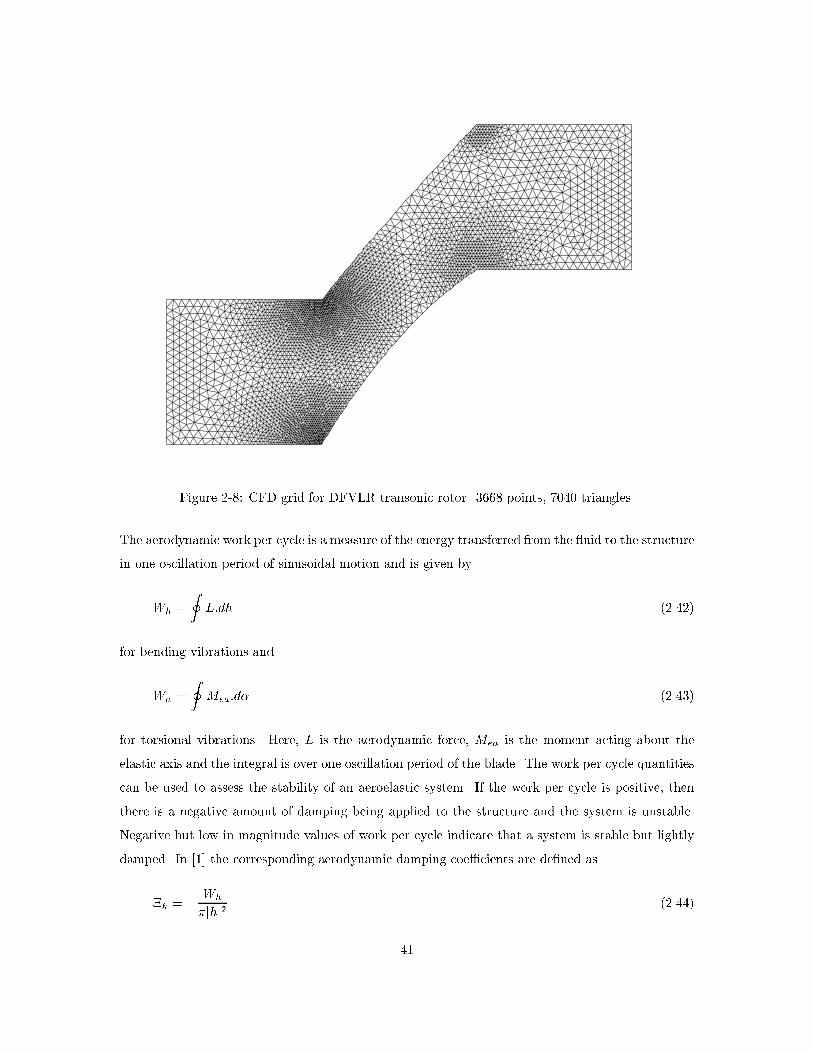
Figure ���� CFD grid for DFVLR transonic rotor� ���� points� ���� triangles�

The aerodynamic work per cycle is a measure of the energy transferred from the �uid to the structure

in one oscillation period of sinusoidal motion and is given by

Wh �

IL�dh ����

for bending vibrations and

W� �

IMea�d� ����

for torsional vibrations� Here� L is the aerodynamic force� Mea is the moment acting about the

elastic axis and the integral is over one oscillation period of the blade� The work per cycle quantities

can be used to assess the stability of an aeroelastic system� If the work per cycle is positive� then

there is a negative amount of damping being applied to the structure and the system is unstable�

Negative but low in magnitude values of work per cycle indicate that a system is stable but lightly

damped� In �� the corresponding aerodynamic damping coe�cients are de�ned as

'h � � Wh

jhj� ����

��

Figure ���� Steady�state pressure contours for DFVLR transonic rotor� M � ����� � � ������

and

'� � � W�

j�j� � ����

The aerodynamic damping was evaluated as a function of interblade phase angle using the CFD

analysis and is plotted in Figure ���� along with the experimental data from �� � The aeroelastic force

coe�cients were determined experimentally as the transfer functions between the imposed vibratory

motion and the measured lift or moment� The imaginary part of these coe�cients is a measure of

the aeroelastic damping� Figure ���� shows a good correlation with the experimental data� The

agreement obtained is much better than that shown in �� for other analytic and computational

methods�

��� Structural Model

So far the computational model for the aerodynamic governing equations has been presented� In

���� we also require a model which describes the evolution of the structural states� This could be a

��

0

0.5

1

1.5

2

2.5

Cp

Figure ����� Pressure distribution for DFVLR transonic blade� experimental data points and CFDresults lines� M � ����� � � ������

complicated model� such as a �nite element analysis which describes the general deformations of each

blade� or a simple model such as a low�order mass�spring system� Here� each blade is allowed just two

structural degrees of freedom pitch and plunge� The structural equations governing this motion

can be derived by considering a simple mass�spring�damper model with two degrees of freedom as

shown in Figure ����� For a blade with mass per unit length m and chord c� the equations of motion

can be written in non�dimensional form as

���������

M� � � � �

� M� � � �

� � � � �

� � � � �

� � � � Mr

���������

���������

(q�

(q�

�

�

(qr

���������

�

���������

C� � � � �

� C� � � �

� � � � �

� � � � �

� � � � Cr

���������

���������

&q�

&q�

�

�

&qr

���������

�

���������

K� � � � �

� K� � � �

� � � � �

� � � � �

� � � � Kr

���������

���������

q�

q�

�

�

qr

���������

�

���������

L�

L�

�

�

Lr

���������� ����

��

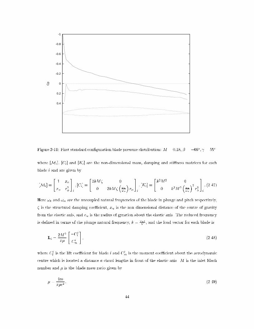
-1

-0.8

-0.6

-0.4

-0.2

0

0.2

0.4

Cp

Figure ����� First standard con�guration blade pressure distribution� M � ����� � � ����� � � ����

where �Mi � �Ci and �Ki are the non�dimensional mass� damping and sti ness matrices for each

blade i and are given by

�Mi �

�� x�

x� r��

�i

� �Ci �

��kM �

� �kM��h��

�r�

�i

� �Ki �

�k�M� �

� k�M���h��

��r��

�i

� ����

Here h and � are the uncoupled natural frequencies of the blade in plunge and pitch respectively�

is the structural damping coe�cient� x� is the non�dimensional distance of the centre of gravity

from the elastic axis� and r� is the radius of gyration about the elastic axis� The reduced frequency

is de�ned in terms of the plunge natural frequency� k � �hcV � and the load vector for each blade is

Li ��M�

�

��Cil

Cim

�� ����

where Cil is the lift coe�cient for blade i and Ci

m is the moment coe�cient about the aerodynamic

centre which is located a distance a chord lengths in front of the elastic axis� M is the inlet Mach

number and � is the blade mass ratio given by

� ��m

�c�� ����

��

-1

-0.8

-0.6

-0.4

-0.2

0

0.2

0.4

0.6

0.8

1-150 -100 -50 0 50 100 150

Aer

odyn

amic

dam

ping

coe

ffici

ent

Interblade phase angle

ExperimentInviscid CFD analysis

Figure ����� First standard con�guration� torsional aerodynamic damping coe�cient as a functionof interblade phase angle� M � ����� � � ����� k � ������

By using the identitiesdhjdt � &hj and

d�jdt � &�j � the structural system ���� can be written as a �rst

order system as follows

du

dt� Su � Ty� ����

where ui � �qi &qi as in the aerodynamic system ����� y contains the aerodynamic force and

moment coe�cients for each blade� and the matrices S and T follow from ����� We note that in

reality� the rotation of the rotor will a ect the structural system as de�ned in ����� However� for

the purpose of this simple structural analysis� this will be ignored�

��� Coupled Aerodynamic�Structural Model

Equation ���� shows the coupling between the aerodynamic and structural models� To determine

the structural states� it is necessary to know the instantaneous aerodynamic forces and moments

acting� These forces depend on the aerodynamics states� which in turn require the blade motion u

��

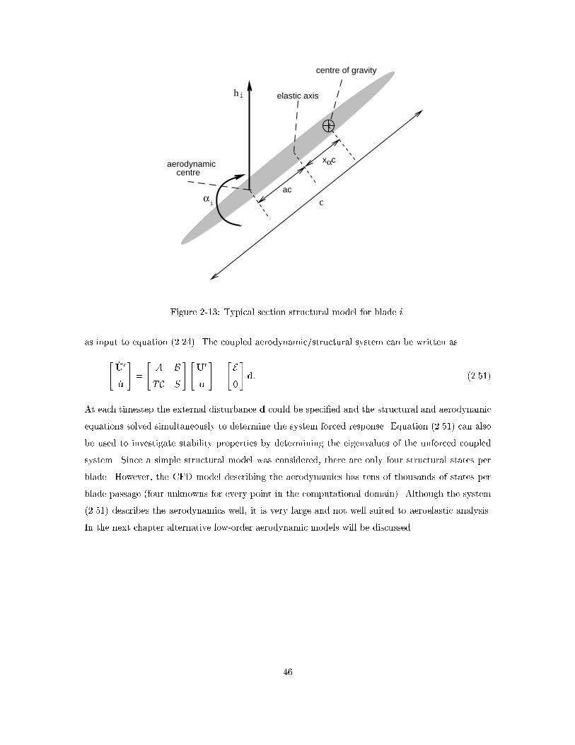
ac

αx c

hi

αi

elastic axis

centre of gravity

aerodynamic centre

c

Figure ����� Typical section structural model for blade i�

as input to equation ����� The coupled aerodynamic�structural system can be written as

�&U�

&u

��

� A BTC S

� �U�

u

��

� E�

�d� ����

At each timestep the external disturbance d could be speci�ed and the structural and aerodynamic

equations solved simultaneously to determine the system forced response� Equation ���� can also

be used to investigate stability properties by determining the eigenvalues of the unforced coupled

system� Since a simple structural model was considered� there are only four structural states per

blade� However� the CFD model describing the aerodynamics has tens of thousands of states per

blade passage four unknowns for every point in the computational domain� Although the system

���� describes the aerodynamics well� it is very large and not well suited to aeroelastic analysis�

In the next chapter alternative low�order aerodynamic models will be discussed�

��

Chapter �

Reduced�Order Aerodynamic

Modelling

While the CFD model described in the previous section provides an accurate representation of the

�ow aerodynamics� the set of ordinary di erential equations obtained is extremely large� There are

four unknowns at each grid point in the computational domain� so the system size is typically of the

order of tens of thousands of unknowns per blade passage� The aeroelastic model ���� is so large

that it is not at all well suited to stability analysis or to control design� It is therefore desirable to

develop a model which still provides an accurate description of the relevant system aerodynamics

but which has only a few states� Such a model would not only be e�cient for solving unsteady �ow

problems� but would also provide an excellent framework for coupling with global engine models and

for control design�

Low�order models have been proposed that fall into essentially two categories� The �rst is to obtain

a model by making simplifying assumptions about the physics of the problem� For example� the �ow

may be assumed to be incompressible and two�dimensional� while the blades can be regarded as �at

plates� These assumptions lead to low�order actuator�disc methods which can be solved analytically�

such as that developed in ��� � While the simpli�ed�physics models often provide insight to a given

problem� and have been widely used� the assumptions involved are generally very restrictive� More

general models can be obtained via the second approach which involves model order reduction of

a high�order CFD method� Within this category� there are again two possibilities� The �rst is to

simplify the CFD model by computing the system response at particular �ow conditions� The overall

��

response is then characterised in terms of constant coe�cients which represent the CFD solution at

these assumed conditions but which are used to provide the aerodynamic model for all �ows� These

methods are referred to as �assumed�frequency� or �in�uence coe�cient� models� Alternatively� one

can systematically reduce the order of CFD method by projecting it onto a reduced�order subspace�

thus restricting its range of validity� In some sense� the assumed�frequency methods are a subset of

this approach� since by restricting the CFD model to a single �ow condition� they compute a model

of the lowest possible order constant coe�cients� The idea of systematic model order reduction is

to increase the number of states in the low�order model thereby preserving a larger range of validity�

Aerodynamic in�uence coe�cient models have been used in many turbomachinery aeroelastic ap�

plications� for example in ���� �� �� �� � The response is calculated from a CFD model by imposing

sinusoidal motion on the blade at a particular frequency often the blade natural frequency� These

aerodynamics are then assumed to represent the system for all �ows� In practice� a signi�cant

amount of coupling often exists between the �ow and the structure� as will be demonstrated in this

chapter by some typical examples� In this case the blade response will contain a range of frequen�

cies and an in�uence coe�cient model cannot accurately represent the system dynamics� Instead�

a high��delity� low�order model which is valid over a range of frequencies can be obtained by pro�

jecting the CFD model onto a set of basis vectors� These vectors are chosen carefully so that the

relevant system dynamics can be well represented with a small number of states� the �e�ciency� of

the model can be characterised by the number of states required to accurately capture the relevant

dynamics� Reduced�order models developed in this manner can be easily cast into state�space form

and hence lend themselves naturally to control design problems�

An in�uence coe�cient model derived from the linearised CFD model of Chapter � will be presented

in this chapter� along with some other options for constructing reduced�order models� There are

several alternatives available for choosing the basis vectors� some of which will be discussed in this

chapter� One is to derive a set of vectors which depend on the system operator� that is a set of vectors

which depend on the large linearised matrix A in equation ����� Eigenmodes are well known as an

e�cient means of representing a solution over a given frequency range� and have been widely used

in modal analyses for structural problems and also for aerodynamic reduced�order modelling ��� �

However to calculate eigenmodes for a large� complex problem can be di�cult� An alternative is

to use the singular vectors of the system which are easy to compute� however these vectors do not

possess the modal character of the eigenvectors and there is no guarantee that the required dynamics

can be captured with a reduced set� Another option is to construct a set of vectors based on the

solution characteristics of the problems under consideration� The proper orthogonal decomposition

��

��� �� is a method for extracting modal information based on simulations of the system� The

�nal method which will be discussed is based on spanning Krylov subspaces of the matrix A� This

approach is related to the eigenmode models and includes the POD as a special case�

��� Aerodynamic Inuence Coecients

The �rst method of CFD model order reduction that will be described is an assumed�frequency

approach� The high�order aeroelastic CFD model ���� will be used to calculate the blade response

to a particular prescribed set of inputs� This calculation results in a set of in�uence coe�cients

which are coupled to the structural model and assumed to represent the response for all �ows� For

blade motion� these in�uence coe�cients represent the magnitude of the forces generated on each

blade due to an imposed unit sinusoidal motion on one blade and all other blades �xed� For external

forcing� they represent the forces generated on each blade due to a unit sinusoidal disturbance in the

appropriate �ow quantity� Although coe�cients must be constructed for each of the r blades being

perturbed in turn� the calculation need only be performed for the �rst blade� with the remaining

r � � cases obtained through symmetry considerations�

Consider the calculation for plunging motion those for pitching motion and external disturbance

follow analogously� We impose a unit sinusoidal motion at a particular frequency� c� on the �rst

blade� and �x all other blades �

h� � ei�ct�

hj � � j � �� �� � � � � r� ���

Although the motion is written as a complex quantity� this is done for convenience and it is only the

real part which is relevant� The analysis can be completed more easily using complex quantities�

and then the real part of the �nal answer taken�

The linearised CFD model ���� could be used to obtain the amplitude of the force acting on

each blade under these conditions� This would involve performing a time simulation of the large

linearised system for the entire bladed disk� The calculation can be performed much more e�ciently

by exploiting the linearity of the governing equations and performing a modal analysis as described

in Section ������ The blade motion h already contains a single temporal frequency� and can be

further decomposed into a �nite set of orthogonal spatial Fourier modes� The component of motion

��

corresponding to spatial mode j is given by hj and has an interblade phase angle of �j � � j�r�

Since ���� is linear� the force contribution due to each hj can be computed separately and then

summed together over all j to obtain the overall force acting�

Consider the imposed blade motion given by ���� Applying the inverse of the transformation ����

to obtain the modal components of this motion� we �nd

hj ��

rj � �� �� �� � � � � r � �� ���

and note that since ��� represents a discrete spatial delta function� the Fourier transform ��� is

a constant� The response due to each of the spatial modes can then be determined by solving the

complex frequency domain Euler equations ���� on a single blade passage� requiring a total of r

solves for each set of in�uence coe�cients� Recombining the results for each spatial mode via �����

we obtain the complex force amplitude L acting on each blade due to sinusoidal motion of blade

one� The instantaneous force acting on blade j due to motion of blade one can therefore be written

as

Lj�t ��LR

j� � iLI

j�

�h�t� ���

where LR

and LI

represent the real and imaginary parts of L respectively� In order to obtain real

coe�cients which can be implemented in the time domain� we note that for the assumed sinusoidal

motion� blade velocity is related to blade displacement via &h � ich� Equation ��� can therefore

be written as

Lj�t � LRj�h�t �

LR

j�

c&h�t ���

and used in an in�uence coe�cient model to represent the force generated on blade j due to any

general motion of blade one� However� due to the assumptions made in obtaining the coe�cients�

the representation for non�sinusoidal motions will obviously contain inaccuracies�

The procedure to calculate the in�uence coe�cients can be summarised as follows� Firstly� for each

type of blade motion impose a unit motion on blade one which varies sinusoidally with time at

the assumed frequency c� and �x all other blades� Next� decompose this motion into its r spatial

Fourier modes and compute the resulting �ow for each mode separately by solving the complex

system ���� a total of r times� Each of these contributions is then summed over the full rotor

using ���� to determine the overall �ow response and the resulting aerodynamic force on each

blade� This produces the in�uence coe�cients for motion of blade one� Finally� the coe�cients for

��

subsequent blades can be obtained via symmetry� that is noting that the force on blade n due to

motion at blade m is identical to the force on blade n�p due to motion at blade m�p� Coe�cients

for external disturbances are computed in an analogous way� noting that allowable spatial frequencies

�j now hold for any integer value of j� In practice� a �nite set of values of spatial frequency are

chosen which are representative of the expected disturbances� These in�uence coe�cients are then

used to represent the aerodynamics in equation ���� for all �ows� not just sinusoidal motions at

c�

��� Reduction Using Congruence Transforms

Although the aerodynamic in�uence coe�cient method provides a means of obtaining low�order�

high��delity aerodynamics� the resulting model is only precise for sinusoidal motions at the assumed

frequency� and has an unknown region of validity for other similar in frequency content and forcing

shape �ows� Interaction between the aerodynamics and structure often excites a signi�cant range of

temporal frequencies and damping in the blade aeroelastic response� and in many turbomachinery

�ows a high degree of coupling or blade�to�blade variations may be present� in which case these

simple models are inadequate� Also� non�sinusoidal forcing inputs may often be of interest� An

alternative approach is to take the high�order linear CFD model ���� and project it onto a set of

e�cient basis vectors to create a low�order model which captures the relevant high��delity dynamics

over a range of frequencies�

It is desirable to choose an orthogonal set of vectors� since the resulting congruent transformation

preserves the system de�niteness� and therefore often preserves system stability� If the set of q

orthonormal basis vectors are contained in the columns of the matrix Vq � a qth order approximation

to the perturbation solution can be made by assuming

U� � Vqv� ���

where vt is the reduced�order aerodynamic state vector� Substituting this representation of U�

into the linearised governing equations ����� we obtain the reduced�order system

dv

dt� V T

q AVqv � V Tq Bu� V T

q Ed� ���

Writing the reduced�order matrix as A � V Tq AVq � it is clear from ��� that the de�niteness of the

��

original system has been preserved� Consider an arbitrary vector w� then

wTAw � wTV Tq AVqw � Vqw

T A Vqw � ���

Therefore if the original matrix A yields strictly positive results from a quadratic form such as ����

so will the reduced system matrix A� This is the de�nition of positive de�niteness� an analogous

statement can be made for negative de�niteness and we also note that inde�nite matrices remain

inde�nite� A negative semide�nite matrix implies that all the eigenvalues have non�positive real part

and the aerodynamic system is stable� In this case� the model reduction will preserve the stability

properties of the system� Many representations involve the computation of two sets of vectors� a

right set Vq and a left set Wq � where Vq and Wq are orthogonal� In this case� the reduced�order

system becomes

dv

dt� W T

q AVqv � W Tq Bu� W T

q Ed ���

and in general the de�niteness of the matrix is not preserved� Unfortunately in the aerodynamic

governing equations considered here� it is not possible to determine the de�niteness of the system

matrix� The result ��� is therefore of limited use in this context�

��� Eigenmode Representation

A reduced�order model can be obtained by computing the eigenmodes of the large linear system

���� and selecting just a few to form a basis� This approach has been taken for many problems�

especially in structural dynamics where the matrices are generally symmetric and the eigenmodes

are easy to compute� Typically the modes with low frequencies are chosen� A large error can result

from the omission of the higher frequency modes� especially if the forcing contains a signi�cant

high�frequency component� This error can be reduced by using a static correction as discussed in

��� � Eigenmodes have been used to form reduced�order models in many applications� While they

may in practice form a very e�cient basis� they are very expensive and di�cult to compute for such

large systems� even in a two�dimensional analysis�

To describe the di�culties associated with the computation of eigenvalues in a turbomachinery con�

text� an attempt was made to calculate the eigenmodes of the system ���� for the subsonic rotor

described in Section ������ The numerical package ARPACK was used for the eigenvalue computa�

tions ��� � This software uses the Implicitly Restarted Arnoldi Method and is appropriate for sparse

��

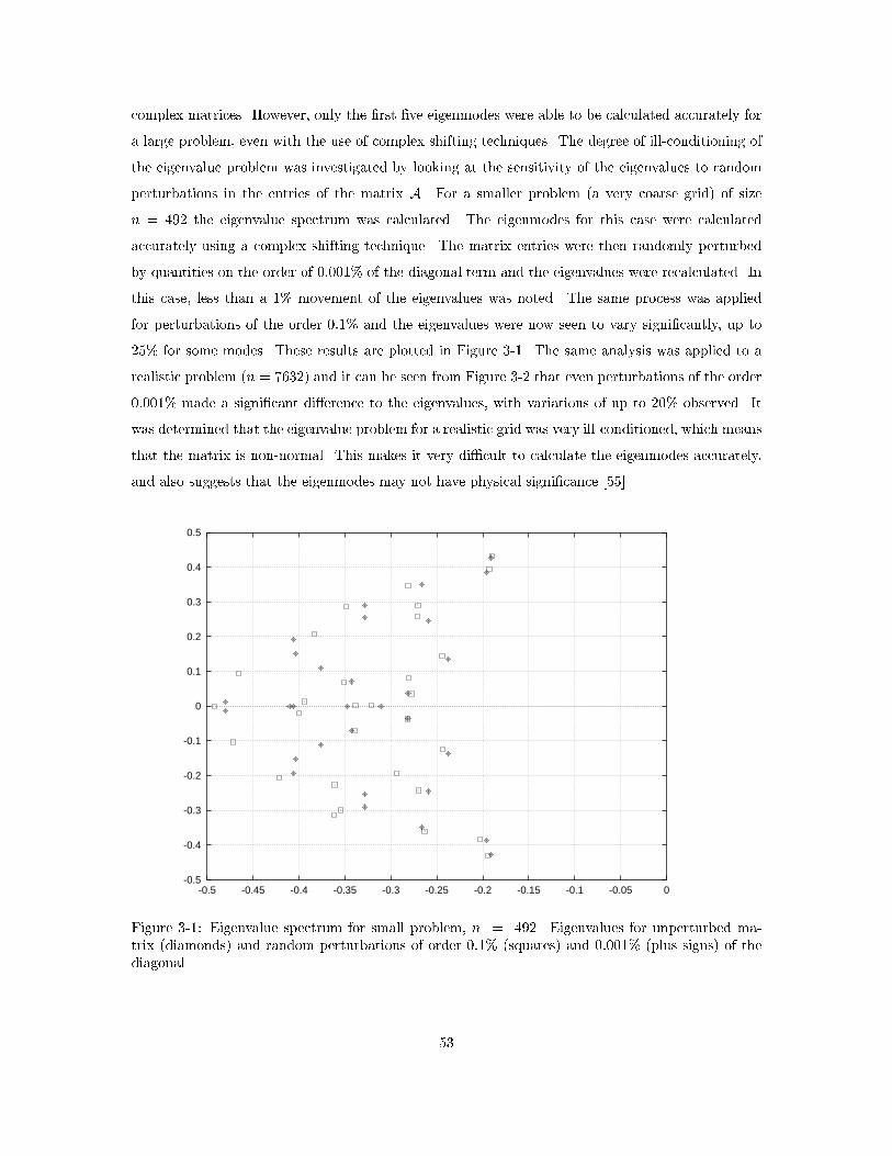
complex matrices� However� only the �rst �ve eigenmodes were able to be calculated accurately for

a large problem� even with the use of complex shifting techniques� The degree of ill�conditioning of

the eigenvalue problem was investigated by looking at the sensitivity of the eigenvalues to random

perturbations in the entries of the matrix A� For a smaller problem a very coarse grid of size

n � ��� the eigenvalue spectrum was calculated� The eigenmodes for this case were calculated

accurately using a complex shifting technique� The matrix entries were then randomly perturbed

by quantities on the order of ������ of the diagonal term and the eigenvalues were recalculated� In

this case� less than a �� movement of the eigenvalues was noted� The same process was applied

for perturbations of the order ���� and the eigenvalues were now seen to vary signi�cantly� up to

��� for some modes� These results are plotted in Figure ���� The same analysis was applied to a

realistic problem n � ���� and it can be seen from Figure ��� that even perturbations of the order

������ made a signi�cant di erence to the eigenvalues� with variations of up to ��� observed� It

was determined that the eigenvalue problem for a realistic grid was very ill�conditioned� which means

that the matrix is non�normal� This makes it very di�cult to calculate the eigenmodes accurately�

and also suggests that the eigenmodes may not have physical signi�cance ��� �

-0.5

-0.4

-0.3

-0.2

-0.1

0

0.1

0.2

0.3

0.4

0.5

-0.5 -0.45 -0.4 -0.35 -0.3 -0.25 -0.2 -0.15 -0.1 -0.05 0

Figure ���� Eigenvalue spectrum for small problem� n � ���� Eigenvalues for unperturbed ma�trix diamonds and random perturbations of order ���� squares and ������ plus signs of thediagonal�

��

-0.8

-0.6

-0.4

-0.2

0

0.2

0.4

0.6

0.8

1

-1 -0.8 -0.6 -0.4 -0.2 0

Figure ���� Eigenvalue spectrum for large problem� n � ����� Eigenvalues for unperturbed matrixplus signs and random perturbations of order ������ diamonds of the diagonal�

In addition� for a non�symmetric problem as in the system considered here� both the right eigen�

vectors Vq and the left eigenvectors Wq must be computed� Although this is not a congruent

transformation� a basis is obtained which preserves system stability� since the eigenvalues of the

reduced�order model are a subset of the original system eigenvalues� This can be seen by noting

that the reduced system matrix is

A � W Tq AVq � )q� ���

where )q is a diagonal matrix whose entries are the eigenvalues corresponding to those eigenvectors

included in the basis Vq �

Other orthogonal sets can be computed more easily� for example the singular vectors of the matrix�

however these lack the e�ciency of the eigenvectors and a very large number may be required to

obtain reasonable solutions� A reduced�order model was constructed using the right singular vectors

as a basis and it was determined that several hundred modes per interblade phase angle were required

to capture the relevant �ow dynamics accurately�

��

��� Proper Orthogonal Decomposition

The POD is a popular alternative to the eigenmode approach for determining an e�cient basis�

Typically� a time simulation of the system for a characteristic unsteady �ow is performed and

instantaneous solutions or snapshots are obtained at selected times� These snapshots are then

combined to produce an orthogonal set of basis vectors which represents the solution U� in some

optimal way� The criterion for choosing the basis vectors was �rst posed in variational form in ��� �

Here we consider choosing the basis vectors � so as to maximise the following cost �� �

max�

hjU�� j�i �

�hjU���j�i

���� ����

where U��� denotes the scalar product of the basis vector with the �eld U�x� t and h i represents

a time�averaging operation� Equation ���� can be rewritten as a constrained optimisation problem

max������

hjU�� j�i� ����

We can then form the Lagrangian function

L � � � hjU�� j�i � � � � � � � ����

where � is the Lagrange multiplier for the constraint on the norm of the basis vector� By di erenti�

ating ���� and setting the result to be zero� we obtain that the function � providing the maximum

in ���� is an eigenfunction of the kernel K de�ned by

Kx�x� ��

n

nXi��

U�ixU�

ix�� ����

where U�ix is the instantaneous perturbation �ow �eld at a time ti and the number of snapshots

n is su�ciently large ��� � The eigenvectors of K are of the form

� �

nXi��

BiU�i� ����

where the constants Bi can be seen to satisfy the eigenvector equation

CB � )B ����

and C is now the correlation matrix constructed by forming inner products between the snapshots

Cij ��

nU�

i�U�j � � i � n� � � j � n� ����

��

It can also be shown �� that the maximum in ���� is achieved and the eigenfunction obtained

corresponds to ��� the largest eigenvalue of C�

The procedure to calculate the POD basis vectors can be summarised as follows� A set of n snapshots

characterising problems of interest is obtained and used to calculate the correlation matrix C de�ned

by ����� The eigenvalues �i and eigenvectors ai � ��i��i� � � � �

in T of C are computed and ordered

according to the size of the real eigenvalues� �� � �� � � � � � �n� Now the basis vectors �i are

chosen as linear combinations of the snapshots� namely� �i �Pn

j�� �ijU

�j � Then for any q� we

represent the solution as a linear combination of basis vectors

U�x� t �

qXi��

vit�ix� ����

The magnitude of the ith POD eigenvalue �i determines the amount of ��ow energy� hU��U�icontained in the ith basis vector� and since

qXi��

hjvitj�i �

qXi��

�i� ����

for a given number of modes the POD is optimal for reconstructing a signal U�x� t in the sense that

the subspace spanned by the resulting vectors �i minimizes the �averaged energy� or the ��norm

of the error between the exact and projected data�

����� Snapshot Generation

Typically in a POD approach of the form described� a time simulation of the full system is run which

is characteristic of the types of �ows we wish to analyse and control� In this simulation certain modes

of the system are excited� and the POD analysis captures this information as snapshots are taken

at di erent instants in time� It is therefore crucial that the important system dynamics are excited

in the sample simulation� This raises an issue if the reduced�order model is to be used for control�

since the idea in controlling a system is the change the nature of the system dynamics� If the POD

analysis is performed on the uncontrolled system� then the modes captured could be completely

di erent from the important dynamics of the controlled system� and the reduced�order model will

not accurately represent the controlled system ��� � Also� the time�marching simulation of the full

bladed disk is an expensive computation�

A more convenient approach is to use linearity and the frequency domain to address some of the

problems associated with the time�domain POD method� The frequency�domain form of the Euler

��

equations was discussed in the previous chapter� The forcing and aerodynamic response is de�

composed into spatial and temporal Fourier modes and the snapshots for each of these modes are

obtained separately� A conventional POD analysis on a motion which contains just a single temporal

frequency shows that only two independent modes exist� The harmonic motion can be completely

reproduced with a linear combination of these two modes� We also note that a harmonic motion

can be completely described by a complex magnitude vector as in �����

U� � Uei�t � UR cost�UI sint � iUI cost �UR sint� ����

Rather than obtaining the snapshots from a time simulation of each harmonic component of the

forcing� for each spatial frequency �j we pick a set of sample temporal frequencies k and solve

the frequency domain equations ���� on a single passage to obtain the complex solution Ujk

� We

then take the real and imaginary parts of this solution as snapshots for the POD process� If the

complex solution for frequencies �j and k has real and imaginary parts UR and UI respectively�

the snapshots for the full rotor are constructed as follows�

U� �

����������������

UR

UR cos�j �UI sin�j

UR cos ��j �UI sin ��j

� � �

UR cos r � ��j �UI sin r � ��j

����������������

����

and

U� �

����������������

UI

UI cos�j �UR sin�j

UI cos ��j �UR sin ��j

� � �

UI cos r � ��j �UR sin r � ��j

����������������� ����

Because we are working in the frequency domain and the forcing contains a single spatial frequency�

all complex solves are made on just a single passage� The frequency domain approach is there�

fore much more e�cient than sampling in the time domain� Additionally� we are picking relevant

frequency content when choosing the basis vectors� rather than modes which are excited under a

certain type of forcing� If it is possible to assess what range of frequencies will be present in both

the uncontrolled and the controlled response� then a reduced�order model can be constructed which

represents both sets of system dynamics�

��

The quality of the reduced�order model is highly dependent on the arbitrary choice of sample

frequencies� Careful consideration needs to be given to ensure that the range sampled spans all

important frequencies in problems of interest� and also that a su�ciently high number of frequencies

within this range are included� Although much more e�cient than a time domain POD analysis�

this model requires the large matrix �ik �Aj to be factored for each pair of snapshots� If a large

frequency range needs to be considered� the cost of generating the model can become high�

��� Arnoldi�Based Model Order Reduction

In this section� an approach will be developed which is related to the eigenmode approach and

includes the POD method as a special case� A set of Arnoldi vectors is used to construct the basis

��� � The Arnoldi vectors approximate the eigenvectors ��� but are much more straightforward to

compute� The full set of Arnoldi vectors spans the same solution space as the system eigenvectors�

a reduced set of q vectors spans the qth order Krylov subspace� The approach also contains some

�avour of the POD in that an e�cient reduced set can be constructed by considering inputs and

outputs of interest� While the basis is easy to compute� some of the issues associated with the

sampling requirements in the POD are addressed� Pad!e�based reduced�order models have been

developed for linear circuit analysis using the Lanczos process ��� � This approach matches as many

moments of the system transfer function as there are degrees of freedom in the reduced system�

While the Arnoldi vectors match only half the number of moments as the Pad!e approximation� they

preserve system de�niteness and� as discussed in Section ���� in the case of a stable negative de�nite

system therefore preserve stability ��� � The Arnoldi vectors are also much cheaper to compute than

the Pad!e vectors�

Our basic goal is to obtain a reduced system which has many fewer states than the original system�

but which still represents the original system�s dynamics accurately� One approach to ensuring

accurate representation of system dynamics would be to try to match the transfer functions of the

reduced and the original systems� This would enable us to replicate the output behaviour of the

high�order CFD model for a range of inputs� Consider �rst a single input� single output system

&U� � AU� � bu� y � cTU�� ����

We note that if the output de�nition were to include direct transmission terms of the form Du or

Fd� these would not a ect the model order reduction procedure� The transfer function between

��

input ut and output yt is

Hs � cT sI �A��b� ����

which can also be represented as a rational function

Hs �Ns

Ds�

bn��sn�� � bn��s

n�� � � � � � b�s � b�ansn � an��sn�� � � � � � a�s � �

� ����

where n is the dimension of the high�order system ����� A qth order Pad!e approximation to the

transfer function is obtained by retaining q coe�cients in each of the polynomials Ns and Ds as

follows�

Hqs �%bq��s

q�� � � � � � %b�s � %b�%aqsq � %aq��sq�� � � � � � %a�s � �

� ����

The �q coe�cients %aj and %bk are selected so as to match the coe�cients of the �rst �q terms in a

McLaurin expansion of the transfer function ����� We can write

Hs � ��Xk��

mksk� ����

where the kth coe�cient

mk � cTA��k�b ����

is the kth moment of Hs� By equating ���� and ����� and considering each power of s separately�

a system of equations for the %aj and %bk can be obtained� The q Pad!e vectors can be constructed

via the Lanczos process and will therefore lead to a reduced�order system which matches the �rst

�q moments of Hs�

An alternative approach is to use the Arnoldi method to generate a set of vectors which spans the

qth order Krylov subspace de�ned by

KqA�b � spanfA��b�A��b� ����A�qbg� ����

By selecting the sequence of vectors

�� � A��b�

�� � A��b � ���

��

���

�q � A�qb � ������ � � � ��q�� ����

for the basis Vq � a qth order reduced�order model of the form ��� is obtained� In ����� the symbol

� denotes the orthogonalisation of each vector with all previous vectors� This is done by subtracting

the appropriate components� as in a standard Gram�Schmidt orthogonalisation procedure� The q

moments of the transfer function of this reduced system are identical to the �rst q moments of

the original system transfer function� as is proved in ��� � The Arnoldi approach therefore matches

only half the number of moments as the Pad!e approximation� however the basis is much cheaper to

compute� It is possible to reduce systems with multiple inputs using the block Arnoldi method� For

example� if we consider a system with two inputs u� and u��

&U� � AU� � b�u� � b�u�� ����

then the block Arnoldi method is used to generate vectors which span the Krylov subspace

KqA�b��b� � spanfA��b��A��b��A��b��A��b�� ����A�qb��A�qb�� g� ����

We also note that it is not necessarily the �rst q moments of the transfer function which must be

matched� If we were to consider a Taylor series expansion of the transfer function about some non�

zero value of s� a model could be obtained which would give a better approximation of the system

dynamics for higher frequencies� For an expansion about s � i� the jth basis vector has the form

A� i�jb� These multiple frequency point Arnoldi methods are described in ��� �

����� Computation of Arnoldi Basis

In order to calculate the basis� we consider input vectors which correspond to a particular blade hav�

ing a unit displacement or velocity and all other blades �xed� Although vectors must be constructed

for each of the r blades being perturbed in turn� the calculation need only be performed once� with

the remaining r � � vectors constructed through symmetry considerations� Once again we can use

linearity to decompose this forcing into a set of r orthogonal modes each containing a single spatial

frequency via ����� and the calculation for each of these modes can be performed on a single blade

passage� For expansions of the transfer function about s � ik� solutions must be performed of

the complex frequency domain equations ����� The resulting solutions are then combined via the

��

inverse of the transformation ���� to obtain the �rst blade basis vector� Vectors for subsequent

blades are computed through use of symmetry� Further simpli�cation can be obtained by noting

that for expansions about s � �� the set of Arnoldi vectors for spatial frequencies � and �� are

complex conjugates of one another� The algorithm for the single input� single output case expanded

about k is shown below�

Algorithm ��� �Arnoldi Method�

arnoldi�input A�b� k� qk� r� output Vq�

f

for j � �� j �� r � �� j � � f � loop over interblade phase angles

Factor �ik �Aj � most expensive step in the algorithm

Solve �ik �Aj �� � b � first basis vector �� � A��jk b

for k � �� k � qk� k � � f � loop over Krylov subspace directions

Solve �ik �Aj w � �k � subsequent vectors �i � A��jk �i��

for i � �� i �� k� i � � f � orthogonalise wrt previous vectors

h � wT�i � compute projections

w � w � h�i � subtract the projections for orthogonality

g

�k� � w

jjwjj � normalise to get the k � �th basis vector

g

V jq � �������q � qth order basis for jth spatial frequency

gg

����� Arnoldi Approach versus POD

One can see the similarities between the POD approach and the multiple frequency point Arnoldi

method� In fact� solving the system ���� at J frequencies to obtain the POD snapshots results in

��

an identical data set as taking J frequency points and computing a single Arnoldi vector at each

point the subsequent orthogonalisation procedure di ers between the two methods� This can be

seen by noting that the vector which solves the complex system ���� is both the POD snapshot at

the frequency k and the �rst vector in the Arnoldi basis expanded about k� It is postulated that

very e�cient models could be constructed by considering a range of frequencies and using the POD

analysis to choose the basis vectors� but also computing more than one vector at each frequency

as in the Arnoldi approach� One must evaluate the relative gain in choosing a higher number of

frequency points� since by far the most expensive part of the calculation is the factorisation of the

matrix in solving the linear system� In the Arnoldi approach� the matrix is computed and factored

just once for each k and �j � but as outlined in the Algorithm ���� qk vectors are obtained per

factorisation� For the POD a di erent matrix must be factored for every pair of snapshots� and

moreover the number of snapshots typically exceeds the �nal number of basis vectors constructed

by a signi�cant amount�

����� Arnoldi Model Extensions

The Arnoldi method described here could be further extended to produce even more e�cient models�

It would be possible to consider the dual problem� That is� instead of forming vectors which span

the Krylov space KqA�b� we choose vectors which span the dual Krylov space K�qAT � c� This

would involve solving a series of systems of the form ATv � c� In this way more e�cient models can

be obtained if the number of inputs of the original system is greater than the number of outputs�

This is typically the case in aeroelastic analyses� since for each structural degree of freedom there

are two inputs blade position and velocity and just one output aerodynamic force or moment�

For example for plunge� the inputs are h and &h� while the single output is the force on the blade Cl�

This concept could be further extended if both inputs and outputs of interest were included in the

choice of basis vectors� The resulting system could be post�processed using a truncated balanced

realisation to get even more improvement ��� �

��� Projection onto Optimal Basis Vectors

Although we use the frequency domain to obtain the snapshots e�ciently on a single blade passage

whether using the POD or the Arnoldi approach� the reduced�order model is developed in the time

domain for the full rotor� The resulting set of ordinary di erential equations is in �state�space� form

and can therefore be easily incorporated into a general aeroelastic analysis�

��

���� Static Corrections

If eigenmodes are used to form the basis� a signi�cant error can arise due to the high�frequency

modes which are excluded� especially if the forcing function contains a signi�cant component in

these frequencies� This has been well documented for both structural dynamic problems �� and

aerodynamic problems ���� �� � The �mode�displacement� method can be used to reduce this error�

thus allowing accurate models to be constructed with a small number of eigenmodes� The high�

frequency modes can be assumed to respond in a quasi�static way� so that the solution can be

written

U�x� t � Uhomx� t �Uparx� t� ����

The homogeneous part of the solution is projected onto a small number of basis functions

Uhomx� t �

qXi��

vit�ix� ����

while static corrections are derived for blade motion and each type of external disturbance� If we

consider the external �ow disturbance to be in the �th spatial Fourier mode� d�� t � d�teil� �

then the particular solution is

Uparx� t � htUhx � &htU �hx � �tU�x � &�tU ��x � d�tU�� ����

The static correction functions Uh� U �h� U� and U �� are particular solutions of the �ow system and

are precomputed by solving for steady �ows with unit boundary conditions on blade position and

velocity� Similarly� U� is the �th spatial Fourier component of a steady �ow with a unit external

disturbance and is also precomputed�

These corrections are not required for the POD or Arnoldi approaches� since the basis vectors are

selected based on solutions of the �ow system� which already contain the relevant high�frequency

dynamics� In fact� we note that for Arnoldi vectors computed about s � �� the �rst basis vector is

exactly the static correction� although the solution representation is slightly di erent� For example�

if we consider plunge and write the forcing term Bu in ���� as bhh�b �h&h� then the �rst two Arnoldi

vectors satisfy the equations

A�� � bh ����

��

and

A�� � b �h� ����

Equations ���� and ���� represent exactly �ows with a unit blade displacement and velocity

respectively� which are the conditions used to obtain the static corrections� The resulting reduced�

order models have a much simpler form if the static corrections are not used� For completeness�

derivation of reduced�order models both with and without the corrections will be presented�

���� Reduced�Order Models

If no static corrections are used� the reduced�order model is simple to derive� The assumed expansion

for the solution ���� is substituted into the governing equations ����� where the basis vectors �

could be derived from either the POD or the Arnoldi�based approach� Using orthogonality� a system

of ordinary di erential equations for the modal coe�cients is obtained as follows

dvidt

� �Ti A

qXi��

vj�j ��Ti Bu��T

i Ed� ����

The reduced�order model is constructed by considering each pair of interblade phase angles ��separately� and using the fact that solutions at di erent interblade phase angles� since they represent

circumferential Fourier modes� are orthogonal to one another� Since ���� represents a congruent

transformation� the de�niteness of the original matrix A is preserved� as discussed in Section ����

The full state�space system can be written

&v � Av � Bu � Ed y � Cv� ����

where v contains all the modal coe�cients and the A matrix is block diagonal according to interblade

phase angle�

A �

������

�A� � � �

� �A� � �

� � �� � � �

� � � �� � �

������ � ����

This can be seen by noting that for a basis vector �j corresponding to interblade phase angle �j �

the vector A�j also has a spatial frequency of �j since the matrix A is periodic and is the same in

each passage� The value of �Ti A�j in ���� is therefore zero if �j and �i correspond to di erent

��

spatial frequencies� Note also that in ���� the states v correspond to each interblade phase angle�

while the inputs u correspond to each blade�

The output vector y contains quantities of interest� typically the aerodynamic forces and moments

acting on each blade� For r blades the output vector y de�ning aerodynamic forces and moments is

given by

y �

������������������

C�l

C�m

C�l

C�m

���

���

Crl

Crm

������������������

� ����

The matrix C de�nes the output appropriately and is typically a function of the problem geometry�

With the use of static corrections� the system becomes a little more complicated� Substituting the as�

sumed expansions for the perturbation solution ���� and ���� into the governing equations ����

and using orthogonality� a slightly di erent system of ordinary di erential equations is obtained as

follows�

dvidt

� �Ti A

qXi��

vj�j � fi� ����

where the forcing vector f is given by

fit � � &ht�Ti Uh � (ht�

Ti U �h � &�t�

Ti U� � (�t�

Ti U �� � &d�t�

Ti U�� ����

Because the static correction functions are derived for each interblade phase angle� h and � in ����

represent the component of blade displacement corresponding to a particular spatial frequency� In

order to write these in terms of the actual blade displacements� the problem is formulated in a

standing wave representation which allows for arbitrary transient motion of the blades ��� � The

arbitrary motion of r blades uj can be represented as a superposition of r standing wave modes�

For example for plunge displacement� we write

hjt �

r��

�Xr��

�hcrt cos j�r � hsrt sin j�r � ����

��

The two travelling modes corresponding to interblade phase angles � and �� are considered together

to obtain two standing wave modes for each pair� This can be written equivalently in matrix form

as

h � %Phr� ����

where h contains the plunge displacement of each blade as a function of time and hr contains the

so�called multiblade coordinates hcr and hsr� %P is the transformation matrix from standing waves

to blade coordinates and is given by

%P �

�������

� cos ��� sin ��� � � � sin ���r���

� cos ��� sin ��� � � � sin ���r������

������

������

� cosr � ��� sinr � ��� � � � sinr � ���r���

������� ����

The system of ordinary di erential equations ���� can therefore be written

&v � Av � Br%ur � E &d y � Cv � Dr%ur � Fd� ����

where %ur contains the displacement� velocity and acceleration components corresponding to each

standing wave mode and Br and E contain the appropriate forcing terms of ����� The expression

for the output y is obtained by substituting the assumed expansions ���� and ���� into the

linearised output de�nition y � CU�� Using the transformation ���� for each of the standing

wave displacements� velocities and accelerations� we can replace %ur in ���� to obtain the resulting

state�space system

&v � Av � B%u� E &d y � Cv � D%u� Fd� ����

where %u now contains the displacements� velocities and accelerations of each blade� Note that both

qt� which is used for evaluating output� and (qt� which occurs in the forcing term� appear in the

model� Similarly� the forcing term requires the evaluation of &d� The matrix A is still block diagonal

by interblade phase angle� however we now require the matrices C� D and F to de�ne the outputs�

where the extra matrices D and F arise from the representation of the solution ����������

��

�� Reduced�Order Modelling Summary

Currently in aeroelastic analyses� in�uence coe�cients are computed for imposed sinusoidal motion

from a high��delity aerodynamic model� In this way a low order but accurate means of representing

the aerodynamics in ��� is obtained� However these models are only valid at the frequency at

which they were computed� and for a typical system in which the blade response contains a range of

frequencies� these models are insu�cient� The challenge has therefore been to develop aerodynamic

models which are not only low order and high �delity� but which also describe the aerodynamics

over a range of frequencies� This can be achieved via reduced�order modelling in which appropriate

CFD solutions are projected onto a reduced�space basis�

The eigenmodes of the system would be a desirable choice for basis vectors since they depend on

the aerodynamic operator and capture all the possible dynamics� A reduced set can be constructed

by considering only eigenvalues whose frequencies fall within the range of interest� However� eigen�

problems of the type encountered in turbomachinery �ows are too ill�conditioned numerically to be

used� The singular vectors of the system are also operator dependent and are easy to compute�

however it was found that hundreds of vectors per blade passage were required to get an accurate

model� The proper orthogonal decomposition has been used very successfully to construct accurate

models e�ciently� however for a typical bladed disk� the cost of generating the snapshots can be

high if a large frequency range is to be considered� Another issue with the POD approach is that it

is necessary to determine the arbitrary set of sample frequencies� Typically some knowledge will be

available on the range of frequencies expected to be present in the system response� and the POD

will be sampled over this range� However� it is also necessary to choose exactly which frequencies

will be sampled within this range� If samples are placed too far apart� important system dynamics

may be missed� if they are placed too closely together� a large number of matrix factorisations and

solves is necessary� thus the cost of generating the model will be high�

The Arnoldi method provides an excellent alternative to the eigenmode and POD approaches� The

Arnoldi basis has the bene�ts of an eigenmode approach in that it models the dynamics of the

original high�order system� but it is much more straightforward to compute� The basis is selected

according to inputs of interest� which makes it very e�cient� but since several vectors are calculated

at each frequency� the model is much less sensitive to the choice of sample frequencies� The models

are much cheaper to compute than those constructed using the POD since one matrix factorisation

can be used to obtain many basis vectors� Results presented in the next chapter will show that these

reduced�order models can capture the relevant system dynamics accurately with a huge reduction

in the number of states�

��

Chapter �

Reduced�Order Modelling of a

Transonic Rotor

Reduced�order models have been developed for subsonic and transonic cascades undergoing general

pitching and plunging motion� A variety of forced response cases have been considered to validate

the models and determine the size of the resulting reduced�order state�space systems� Results will be

presented in this chapter for the DFVLR L����� transonic rotor discussed in Chapter �� This rotor

is analysed in unsteady plunging motion for a twenty�blade con�guration� Figure ��� shows the grid

for two passages of the rotor� The steady�state �ow has an inlet Mach number of ���� and was shown

previously in Figure ���� A CFD analysis of the full rotor would have ������ unknowns� With the

resources available� routine computations of this size as required for design are not feasible� The

results presented in this chapter will demonstrate that the system dynamics relevant to �utter and

forced response can be accurately captured with less than two hundred states in the reduced�order

model�

��� Aerodynamic Reduced�Order Models

To illustrate the application of di erent model order reduction techniques to a representative prob�

lem� reduced�order aerodynamic models were developed using both the POD and Arnoldi approaches�

��

Figure ���� Computational domain for two passages of the DFVLR transonic rotor� ���� nodes����� triangles per blade passage�

����� POD Reduced�Order Model

To construct the POD model� twenty snapshots were obtained for each interblade phase angle� with

samples being made at ten equally spaced reduced frequencies over the range k � � to k � ���� for

a total of four hundred snapshots� This frequency range represents the low�frequency aerodynamics

which are typically of interest in an aeroelastic analysis� The POD eigenvalue spectra for interblade

phase angles of �� and ���� are plotted in Figure ���� Note the log scale on the plot and the huge

variation between the largest and smallest eigenvalues� The jth POD eigenvalue is an indication of

how much �ow energy is captured by the jth POD basis vector� and so this plot shows that only

the �rst six or eight modes for each interblade phase angle are required to capture almost all of the

system dynamics in this sample set� For these two interblade phase angles� choosing just the �rst six

modes captures over ��� of the �ow energy� The POD eigenvalues for the other interblade phase

��

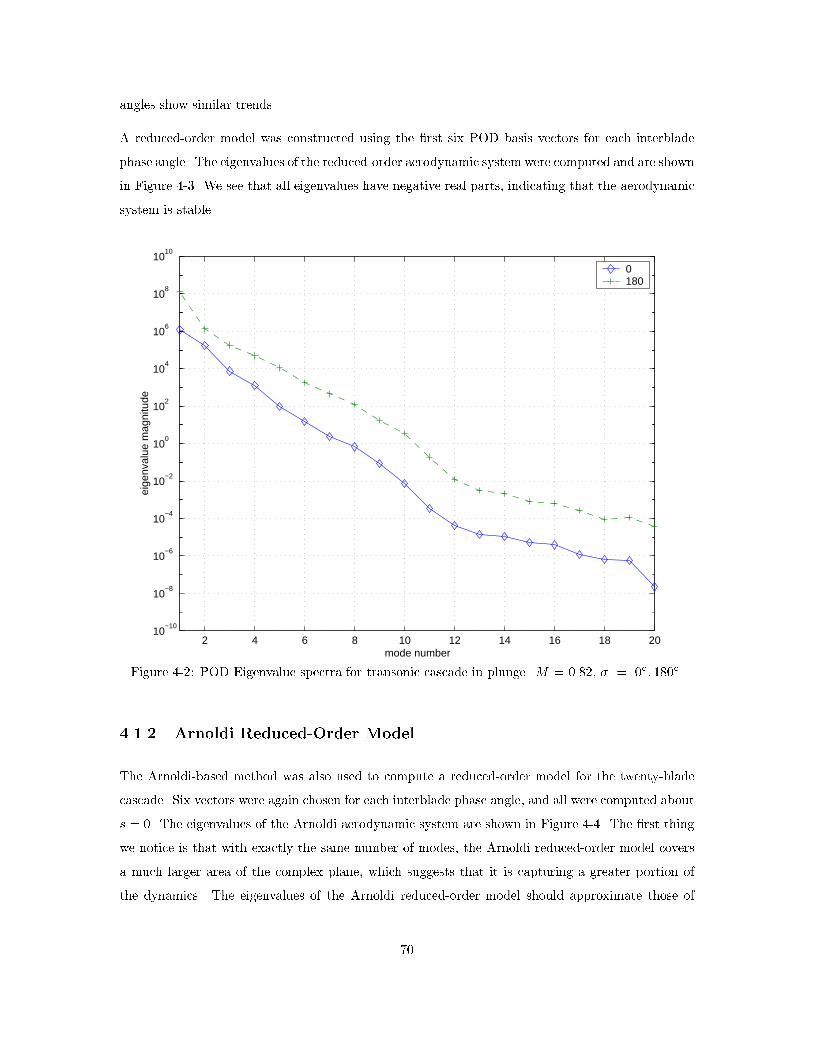
angles show similar trends�

A reduced�order model was constructed using the �rst six POD basis vectors for each interblade

phase angle� The eigenvalues of the reduced�order aerodynamic system were computed and are shown

in Figure ���� We see that all eigenvalues have negative real parts� indicating that the aerodynamic

system is stable�

2 4 6 8 10 12 14 16 18 2010

−10

10−8

10−6

10−4

10−2

100

102

104

106

108

1010

mode number

eige

nval

ue m

agni

tude

0 180

Figure ���� POD Eigenvalue spectra for transonic cascade in plunge� M � ����� � � ��� �����

����� Arnoldi Reduced�Order Model

The Arnoldi�based method was also used to compute a reduced�order model for the twenty�blade

cascade� Six vectors were again chosen for each interblade phase angle� and all were computed about

s � �� The eigenvalues of the Arnoldi aerodynamic system are shown in Figure ���� The �rst thing

we notice is that with exactly the same number of modes� the Arnoldi reduced�order model covers

a much larger area of the complex plane� which suggests that it is capturing a greater portion of

the dynamics� The eigenvalues of the Arnoldi reduced�order model should approximate those of

��

−0.7 −0.6 −0.5 −0.4 −0.3 −0.2 −0.1 0−1.5

−1

−0.5

0

0.5

1

1.5

real

imag

Figure ���� Eigenvalue spectrum for POD reduced�order aerodynamic system� Six modes per in�terblade phase angle total ��� modes�

the original system since the Arnoldi vectors provide a good approximation of the eigenvectors of a

sparse matrix ��� � While the POD model is valid only over the frequency range sampled to obtain

the snapshots and taking more basis vectors does not add any further information as shown by the

POD eigenvalues in Figure ���� as we take more vectors in the Arnoldi basis we expect to obtain

a model which represents a greater portion of the system dynamics� The eigenvalues towards the

left of the plot fall into a distinctive parabolic shape which is typically associated with convective

modes ��� and will be discussed in a subsequent section�

��

−7 −6 −5 −4 −3 −2 −1 0−2

−1.5

−1

−0.5

0

0.5

1

1.5

2

real

imag

Figure ���� Eigenvalue spectrum for Arnoldi reduced order aerodynamic system� Six modes perinterblade phase angle total ��� modes� All basis vectors computed about s � ��

��

��� Aerodynamic Forced Response

One question which must be addressed in the POD approach is that of choosing the sample fre�

quencies� It is necessary to ensure that the appropriate range of frequencies are sampled� and also

that su�cient samples are taken over this range� This question does not arise with the Arnoldi

method� however it is still necessary to determine how many basis vectors must be included in the

reduced�order model to obtain an accurate representation of the relevant system dynamics� Forced

response of the cascade to a pulse input in plunge is a good way of answering both of these questions�

since a pulse contains a continuous spectrum of temporal frequencies� Comparison of reduced�order

model results with the full simulation code will determine both the required size of the reduced�order

models� and also whether enough sample frequencies were used to construct the POD basis vectors�

The input takes the form

ht � e�g�t�t��

���

where g is a parameter which determines how sharp the pulse is and thus the value of the highest

signi�cant frequency present� To determine the frequency content� a Fourier transform of ��� can

be performed� also yielding a Gaussian�

H ��

�p g

ei�t�e���

�g � ���

Since the linearised CFD simulation code is implemented in the time domain� for a general input

the entire rotor would have to be considered� As mentioned� this is not a feasible computation� We

are limited to solving the large system on just one or two blade passages� Accordingly� all twenty

blades were supplied with the same input� which results in a motion containing only an interblade

phase angle of zero� Since the solution will be the same in all passages� the time�domain linearised

simulation can be performed on just a single passage� The input in blade plunge displacement is

shown in Figure ��� for g � ����� The signi�cant frequency content for this value of g is for � ����

k � ����� Above this frequency� the magnitude of the components are less than ������ and therefore

deemed to be insigni�cant� This range of frequencies is well within that sampled by the POD�

The forced response calculated by each of the reduced�order models is plotted in Figures ��� and

��� and in each case is compared to the linearised CFD simulation code� We can see that with just

six modes� both models do a very good job of predicting the response� Although the POD model

calculates the force more accurately with four modes� with six modes it slightly underpredicts the

force at the peaks� while the Arnoldi model is very close to the linearised simulation response� To

��

construct the POD model� twenty snapshots were obtained for � � �� ten matrix factorisations� In

comparison� all the Arnoldi vectors were computed at a single frequency point s � � and so could

be obtained with a single matrix factorisation� For the cases shown here� the POD reduced�order

model was a factor of ten times more expensive to compute than the Arnoldi reduced�order model

ten matrix factorisations versus one� Moreover� the Arnoldi model is as good� if not slightly better�

To further demonstrate the utility of the Arnoldi method� a pulse input with a value of g � ���

was considered� This pulse contains signi�cant reduced frequencies in the range k � � to k � ����

which is slightly outside the range sampled by the POD k � � � � � ����� By computing twelve

Arnoldi basis vectors� a good agreement with the CFD result could be obtained note that very

little computational e ort is required to compute these extra vectors since the matrix factorisation

has already been obtained� For the POD model� it was found that taking more than eight basis

vectors from the existing snapshot database created an unstable model� This is most likely due to

numerical conditioning � beyond the �rst eight modes� the POD eigenvalues become relatively very

small and numerical errors start to become signi�cant� This is apparent through a gradual loss of

orthogonality in the higher modes� To obtain a higher number of useful basis vectors� we would need

to obtain more snapshots and repeat the POD analysis� For the purposes of comparing the existing

available data� the POD reduced�order model was constructed using just eight modes which gives

the best possible result for this snapshot collection� The forced response computed with the CFD

code is plotted in Figure ��� along with results from the Arnoldi reduced�order model with twelve

modes and the POD reduced�order model with eight modes� We see a much better agreement for

the Arnoldi reduced�order model� although� again� both models do a reasonable job with the POD

underpredicting the peak responses� To improve the reduced�order model performance� for the POD

it would be necessary to include the higher frequency range when obtaining the snapshots� which

will signi�cantly increase the required number of system solves� For the Arnoldi� it would be possible

to obtain a lower order model by deriving some of the Arnoldi vectors about a non�zero frequency

point in this case a value near s � ��� might be appropriate�

A case was then considered where just one blade was forced with the pulse input� while all others

were held �xed� This motion contains all possible interblade phase angles� The response for each

blade was computed using the Arnoldi reduced�order model with six modes for � � �� and ten modes

for all other �� The inputs and response of each blade are shown in Figure ���� This computation

was too expensive to be carried out with the linearised simulation code� It is clear from the plot

that the largest force is generated on the disturbed blade and its nearest neighbours� as might be

expected intuitively� We can see that beyond the two closest blades the force generated is very small�

��

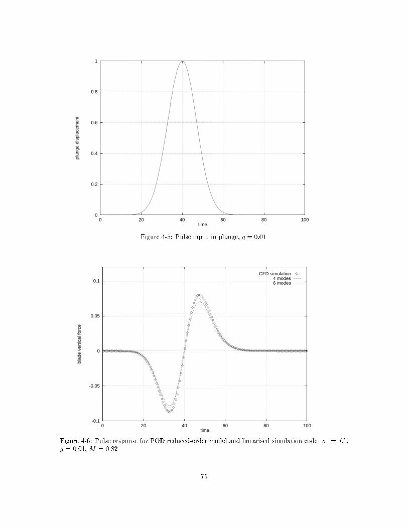
0

0.2

0.4

0.6

0.8

1

0 20 40 60 80 100

plun

ge d

ispl

acem

ent

time

Figure ���� Pulse input in plunge� g � �����

-0.1

-0.05

0

0.05

0.1

0 20 40 60 80 100

blad

e ve

rtic

al fo

rce

time

CFD simulation4 modes6 modes

Figure ���� Pulse response for POD reduced�order model and linearised simulation code� � � ���g � ����� M � �����

��

-0.1

-0.05

0

0.05

0.1

0 20 40 60 80 100

blad

e ve

rtic

al fo

rce

time

CFD simulation4 modes6 modes

Figure ���� Pulse response for Arnoldi reduced�order model and linearised simulation code� � � ���g � ����� M � �����

-0.3

-0.2

-0.1

0

0.1

0.2

0.3

0 5 10 15 20 25 30

blad

e ve

rtic

al fo

rce

time

CFD simulationPOD ROM (8 modes)

Arnoldi ROM (12 modes)

Figure ���� Pulse response for Arnoldi reduced�order model with �� modes� POD reduced�ordermodel with � modes and linearised simulation code� � � ��� g � ���� M � �����

��

0 50 100−1

0

1

blad

e 1

time0 50 100

−1

0

1

blad

e 2

time0 50 100

−1

0

1

blad

e 3

time0 50 100

−1

0

1

blad

e 4

time

0 50 100−1

0

1

blad

e 5

time0 50 100

−1

0

1bl

ade

6

time0 50 100

−1

0

1

blad

e 7

time0 50 100

−1

0

1

blad

e 8

time

0 50 100−1

0

1

blad

e 9

time0 50 100

−1

0

1

blad

e 10

time0 50 100

−1

0

1

blad

e 11

time0 50 100

−1

0

1

blad

e 12

time

0 50 100−1

0

1

blad

e 13

time0 50 100

−1

0

1

blad

e 14

time0 50 100

−1

0

1

blad

e 15

time0 50 100

−1

0

1

blad

e 16

time

0 50 100−1

0

1

blad

e 17

time0 50 100

−1

0

1

blad

e 18

time0 50 100

−1

0

1

blad

e 19

time0 50 100

−1

0

1bl

ade

20

time

Figure ���� Pulse displacement input dashed line and blade lift force response solid line forArnoldi reduced�order model� Six modes for � � �� and ten modes for all other interblade phaseangles total ��� modes� g � ����� M � �����

��

��� Coupled Aerodynamic�Structural Reduced�Order Model

To illustrate the incorporation of the reduced�order models to an aeroelastic framework� the aerody�

namic systems were coupled to a mass�spring�damper structural system as described in Chapter ��

Recall the structural equations written as a �rst order system ����� For plunge only� the structural

equations for each blade can be written

d

dt

�hj

&hj

��

�� �

�kM� ��kM

� �hj

&hj

��

��

�M�

� Cjl

�� ���

or� as in ����� &u � Su�Ty� This structural model is then coupled to the reduced�order state�space

system ���� with no static corrections as follows �

�&v

&u

��

�A B

TC S

� �v

u

��

�E

�

�d� ���

To determine aeroelastic stability� the eigenvalues of this coupled system are evaluated� For forced

response analysis� the structural and aerodynamic equations can be solved simultaneously using

��� to determine the blade displacement and velocity and the aerodynamic forces and moments

acting�

If static corrections are used� the coupling between the aerodynamic and structural models is a little

more complicated� since in ���� the input vector %u contains more quantities than the structural

state vector u� Since the forcing term B%u only involves &q and (q and the output term D%u only

involves q and &q� ���� could be rewritten as

&v � Av � %B &u� E &d y � Cv � %Du� Fd� ���

where u � �q &q T is now the structural state vector� and the matrices %B and %D correspond directly

to B and D in ���� but with the appropriate columns of zeros removed� The coupled system can

then be written

�&v

&u

��

�I � %B

� I

��� �A �

TC S � T %D

��v

u

��

�E &d

Fd

�� ���

To provide an example of an aeroelastic system� an Arnoldi reduced�order aerodynamic model with

��� aerodynamic states was coupled to a structural model with a reduced frequency of k � ����� no

structural damping � � and a mass ratio of � � ���� These structural parameters are typical for

a rotor blade� The eigenvalues of the coupled system ��� are shown in ���� along with the original

��

aerodynamic eigenvalues� We observe some movement of the original aerodynamic eigenvalues due

to interaction with the structure� and also the introduction of forty structural modes with frequencies

around kM � ������ A zoom of these structural eigenvalues is shown in Figure ����� The number

above each structural eigenvalue identi�es the nodal diameter to which it corresponds� For a nodal

diameter �� the corresponding interblade phase angle is �� � � ��r here we have r � �� blades�

If we consider just the structural equation ��� with no aerodynamics� the resulting solution is the

same for all blades� and is a damped in the general case with structural damping sinusoidal motion

at the blade natural frequency� This so�called in�vacuo mode has all structural eigenvalues at the

conjugate points �kM � ikMp

�� �� Coupling in the aerodynamics to equation ��� causes the

structural eigenvalues to move from this point� and so the response of the coupled system contains a

range of frequencies around the damped natural frequency kMp

�� �� The amount of eigenvalue

scattering� and hence the range of frequencies present in the response� depends on the amount of

coupling between the aerodynamics and the structure� By examining the forcing term in equation

��� we see that there are several factors which a ect this coupling� We �rst non�dimensionalise

time in ��� by t � t��kM � so that the equation of motion for blade j can be written

h��j � �h�j � hj ��Cj

l

�k����

and the blade natural frequency is now unity� The size of the forcing term is a ected by both

the aerodynamics and the structural properties of the blades� For systems with a high degree of

aerodynamic coupling� a small motion of the blade will create a large force and the Cjl term will be

relatively large� The structural parameters enter through the natural reduced frequency k and the

blade mass ratio �� For a massive blade high values of �� the aerodynamics do not have a signi�cant

e ect� and the structural eigenvalues will be tightly clustered around the natural frequency� In the

limit � � � an extremely massive blade the aerodynamics will have no e ect on the structure�

and the response will be in the in�vacuo mode� Similarly� we see a higher degree of coupling for

low values of natural frequency� Figure ���� shows that in this case� even though the blade natural

frequency is fairly low� a small degree of aerodynamic coupling is present in the system� For the

most part� the eigenvalues fall very close to the natural frequency� Even the � � � mode� which

exhibits the most coupling� has a frequency shift of less than ���

We can gain some insight to the motion of the structural eigenvalues by considering the work per

cycle of the cascade� The work per cycle was calculated for each interblade phase angle over the

frequency range k � � to k � ��� and is plotted in Figure ����� The work per cycle represents the

aerodynamic damping and hence the relative motion of the real parts of the structural eigenvalues�

The relevant aerodynamic damping to consider is that in the region near the natural frequency�

��

Three slices of the work per cycle surface near k � ���� are shown in Figure ����� This �gure shows

that for reduced frequencies near k � ����� modes six through twelve interblade phase angles ����

though ���� have the most negative values of work per cycle� and the corresponding eigenvalues

in Figure ���� are the most highly damped� Similarly� the work per cycle analysis predicts that the

interblade phase angles close to � � �� are lightly damped� as is also the case in the eigenvalue

spectrum�

To demonstrate forced response prediction� a time�marching simulation of the coupled system was

run with k � ���� and � �� An initial plunge displacement was applied to one of the blades�

then the structural and aerodynamic response for the entire rotor was computed� Figure ���� shows

the resulting displacement and vertical component force for each blade� Clearly the disturbed blade

blade � exhibits the largest response� and induces some motion in nearby blades� The resulting

motion is decaying� although slowly since the coupled system is lightly damped�

−9 −8 −7 −6 −5 −4 −3 −2 −1 0−2.5

−2

−1.5

−1

−0.5

0

0.5

1

1.5

2

2.5

real

imag

Figure ����� Eigenvalue spectrum for Arnoldi reduced�order model� Purely aerodynamic eigenvaluesdiamonds and coupled aerodynamic�structural system plus signs� ��� aerodynamic states� ��structural states� M � ����� � � ���� k � ����� � ��

��

−0.025 −0.02 −0.015 −0.01 −0.005 0

0.2

0.202

0.204

0.206

0.208

0.21

0.212

0.214

real

imag

7

8

6

12

49

11 10

5

13

20

14

1615

19

118

3

172

Figure ����� Zoom of structural eigenvalues� Eigenvalues are numbered by nodal diameter�M � ����� � � ���� k � ����� � ��

��

050100150200250300350

0

0.5

1

−14

−12

−10

−8

−6

−4

−2

0

reduced frequency

interblade phase angle

aero

dyna

mic

wor

k pe

r cy

cle

Figure ����� Aerodynamic work per cycle as a function of interblade phase angle and reducedfrequency for transonic rotor�

��

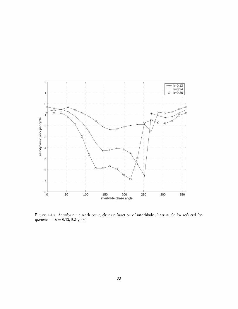
0 50 100 150 200 250 300 350−8

−7

−6

−5

−4

−3

−2

−1

0

1

2

interblade phase angle

aero

dyna

mic

wor

k pe

r cy

cle

k=0.12k=0.24k=0.36

Figure ����� Aerodynamic work per cycle as a function of interblade phase angle for reduced fre�quencies of k � ����� ����� �����

��

0 50 100−2

0

2

blad

e 1

time0 50 100

−2

0

2bl

ade

2

time0 50 100

−2

0

2

blad

e 3

time0 50 100

−2

0

2

blad

e 4

time

0 50 100−2

0

2

blad

e 5

time0 50 100

−2

0

2

blad

e 6

time0 50 100

−2

0

2

blad

e 7

time0 50 100

−2

0

2

blad

e 8

time

0 50 100−2

0

2

blad

e 9

time0 50 100

−2

0

2

blad

e 10

time0 50 100

−2

0

2

blad

e 11

time0 50 100

−2

0

2

blad

e 12

time

0 50 100−2

0

2

blad

e 13

time0 50 100

−2

0

2

blad

e 14

time0 50 100

−2

0

2

blad

e 15

time0 50 100

−2

0

2

blad

e 16

time

0 50 100−2

0

2

blad

e 17

time0 50 100

−2

0

2

blad

e 18

time0 50 100

−2

0

2

blad

e 19

time0 50 100

−2

0

2

blad

e 20

time

Figure ����� Coupled system response to an initial plunge displacement input at blade � � bladedisplacement dashed line and blade vertical force solid line� � � ���� k � ����� � ��

��

��� Comparison of POD with Inuence Coecient Model

In this section� results from a POD reduced�order model will be compared to an in�uence coe�cient

model� The two approaches are very similar in that both models are derived by considering solutions

of the CFD system at frequencies of interest� In fact� the in�uence coe�cient model is a simpli�ed

reduced�order model with just a single snapshot at the blade natural frequency� Since with the POD

we are increasing the cost of deriving the model by considering several frequencies� it is desirable

to determine how much additional accuracy is gained� If the in�uence model is able to capture the

relevant dynamics to the desired level of accuracy� then there would be no reason to develop a more

costly reduced�order model� The ability of each model to capture the dynamics of the coupled system

relevant to predicting �utter and forced response will be assessed� This is achieved by considering

the stability margins of the resulting aeroelastic systems eigenvalues and also the forced response

to an axial velocity disturbance at the passage inlet�

The aeroelastic in�uence coe�cient model has a very simple form� We simply replace the aerody�

namic forces on the right�hand side of ��� with the appropriate coe�cients� Thus the equation for

blade j becomes

(hj � �kM &hj � kM�hj ��M�

�

�rX

k��

��jkhk � �jk &hk

�� �j�d�

����

where �jk � �jk and �j� are the in�uence coe�cients calculated at the assumed frequency� �jk and

�jk represent the force generated on blade j due to a unit plunge displacement and unit plunge

velocity respectively of blade k� Similarly� �j� represents the force generated on blade j due to a

unit disturbance in the �th nodal diameter�

The case chosen for analysis has structural parameters � � ���� k � ���� and � � which are typical

for a compressor rotor blade� The natural frequency of the blade is thus n � kM � ���� A POD

model was generated with snapshots taken at frequencies ��� ��� ���� ���� ���� ���� and ��� percent

of the blade structural frequency� Aerodynamic in�uence coe�cients were calculated at the blade

natural frequency� The eigenvalues of the aerodynamic reduced�order model with four POD modes

per blade passage a total of �� aerodynamic states� and the coupled aeroelastic reduced�order

model with a total of ��� states were computed and are shown in Figure ����� Once again� when

the structural model is coupled in� we see some movement of the original aerodynamic eigenvalues�

plus the introduction of forty structural modes near the natural frequency wn � ���� A zoom of

these structural eigenvalues is shown in Figure ����� along with the eigenvalues for the in�uence

coe�cient model� The numbers on the plot indicate the number of nodal diameters associated with

��

each eigenmode� For � nodal diameters� the corresponding interblade phase angle is �� � � �����

For each interblade phase angle� Figure ���� shows two eigenvalues � that for the reduced�order

model the diamonds and that for the in�uence coe�cient model evaluated at the blade natural

frequency the plus signs� We notice that there is not a particularly high degree of aerodynamic

coupling in the system� since for most modes the eigenvalues do not move far from the natural

frequency of ���� The real and imaginary parts of these eigenvalues are also plotted in Figure ����

for each mode� For the most part� the agreement between the two models is very good� Figure ����

shows that there are two regions where the damping of the modes is not predicted accurately by

the in�uence coe�cient model� The �rst is for the modes whose frequency is far from the natural

frequency modes �fteen through seventeen� while the second is when the damping is high modes

eight through eleven� These cases both represent situations where the actual response conditions

are not close to those assumed in the in�uence coe�cient calculation� When the frequency of

the eigenvalue changes signi�cantly� we would not expect the in�uence coe�cients to capture the

dynamics accurately� because e ectively they have been evaluated at the wrong point� Also� because

the in�uence coe�cient model assumes undamped sinusoidal motion� it cannot capture the system

dynamics accurately when a high degree of damping is present� even if the frequency shift is very

small�

To obtain a better estimation of the dynamics� each in�uence coe�cient should be re�evaluated

at the frequency corresponding to its eigenvalue� although some error will still exist for the highly

damped modes� Coe�cients were recalculated at c � ���� and the resulting eigenvalue for the

� � �� mode is plotted on Figure ���� as an asterisk� The Figure shows that the new eigenvalue has

moved much closer to that predicted by the reduced�order model� In Figure ���� we can see that the

damping of the � � �� mode for the c � ���� model now agrees very closely with the reduced�order

model� but that the damping prediction for the other modes is much worse� since � ���� is a

worse choice of sample frequency for them� If a greater degree of aerodynamic coupling� and thus

more scatter in the modal frequencies existed� the in�uence coe�cient model would not accurately

capture a signi�cant portion of the system dynamics� However the reduced�order model is able to

accurately model the system even when a high degree of coupling exists�

To determine the accuracy of the reduced�order model� the blade force response was calculated for

sinusoidal blade motion over a range of frequencies� and is plotted as solid lines in Figure ���� for

interblade phase angles of ���� ���� and ����� The points on each of the plots are the force calculated

using the linearised CFD model at frequencies corresponding to the POD snapshot sample points�

These values represent the truth model� For interblade phase angles of ��� and ���� the reduced�

��

−2.5 −2 −1.5 −1 −0.5 0−1

−0.8

−0.6

−0.4

−0.2

0

0.2

0.4

0.6

0.8

1

real

imag

Figure ����� Eigenvalues for POD reduced�order model� Purely aerodynamic eigenvalues diamondsand coupled aerodynamic�structural system plus signs� �� aerodynamic states� �� structural states�� � ���� k � ����� � ��

order model does an excellent job of capturing the system dynamics over the entire frequency range�

For ����� a local resonance exists near � ���� which is not fully captured by the reduced�order

model� If more POD modes were included in the model� we would expect to then capture these

dynamics more accurately� The dotted lines on the three plots represent the value of the force which

would be predicted using the in�uence coe�cient model derived at c � ���� Although this model is

exact at this particular frequency� since the dynamics are assumed to be constant it does not capture

any of the important variations with frequency� In addition� the assumption of a sinusoidally time�

varying motion in the in�uence coe�cient model is extremely restrictive� The reduced�order model

can resolve any general motion� provided the relevant frequency range is sampled by the snapshots�

The response of the aeroelastic system to a sinusoidally time�varying axial velocity disturbance at

��

−20 −15 −10 −5 0

x 10−3

0.08

0.085

0.09

0.095

0.1

0.105

0.11

0.115

0.12

0.125

real

imag

01

2 3

4

56

7

89

10 1112

13

14

15

16

17 18

19

AIC w=0.1 ROM AIC w=0.09

Figure ����� Structural eigenvalues for reduced�order model and aerodynamic in�uence coe�cientmodel evaluated at c � n � ���� Also shown is the � � �� eigenvalue for in�uence coe�cientsevaluated at � ����� Structural parameters � � � ���� k � ����� � �� Eigenvalues are numberedby their nodal diameter�

the inlet was then calculated� This disturbance was considered to be in the � � �� spatial mode�

whose dynamics were not well captured by the original in�uence coe�cient model� Figures ���� and

���� show the blade displacement and force response over a range of frequencies for the reduced�

order model and the in�uence coe�cients calculated at c � ��� and ����� The � ��� in�uence

coe�cient model underpredicts the response and also predicts the peak amplitude to be at the wrong

frequency� This is because both the damping and the frequency of the eigenvalue were incorrect� The

recalculated in�uence coe�cients and the reduced�order model agree much more closely� although the

reduced�order model predicts a slightly more damped response at lower frequencies� Even when the

eigenvalue is predicted accurately� the in�uence coe�cient model only predicts the forced response

��

0 2 4 6 8 10 12 14 16 18−0.02

−0.015

−0.01

−0.005

0da

mpi

ng

number of nodal diameters

0 2 4 6 8 10 12 14 16 180.08

0.09

0.1

0.11

0.12

0.13

0.14

freq

uenc

y

number of nodal diameters

ROM assumed frequency w=0.1 assumed frequency w=0.09

Figure ����� Damping and frequency of structural modes for reduced�order model and in�uencecoe�cient models at c � ��� and c � ����� � � ���� k � ����� � ��

exactly at the assumed frequency where �j� in ��� was evaluated� As we move away from the

assumed frequency� an error will be incurred in the forced response calculation� This can be seen in

Figures ���� and ���� since the reduced�order model and in�uence coe�cient model at an assumed

frequency of ���� agree at the assumed frequency but di er away from it� Moreover� if the inlet

disturbance were not sinusoidal in time� the in�uence coe�cient model would be even less accurate�

We note the interesting fact that the force on the blades goes to zero at the blade natural frequency�

yet it is still possible to have a non�zero displacement response� This can be seen by considering

the structural equation ���� For no structural damping� response at � kM is in the blade alone

mode� and the forcing term is zero�

In summary� these results demonstrate that for prediction of �utter and forced response� the situ�

��

0.06 0.08 0.1 0.12 0.14 0.16 0.18 0.2 0.220

0.2

0.4

0.6

0.8

frequency

|F|

0.06 0.08 0.1 0.12 0.14 0.16 0.18 0.2 0.220.5

1

1.5

frequency

|F|

0.06 0.08 0.1 0.12 0.14 0.16 0.18 0.2 0.220

1

2

3

frequency

|F|

Figure ����� Blade force response amplitude to imposed sinusoidal motion� Reduced�order modelprediction solid lines� in�uence coe�cient model prediction dotted lines and CFD solutioncrosses� plus signs and diamonds� From the top � � � ���� � � ���� and � � �����

ation is often such that a simple assumed�frequency method cannot model the relevant dynamics

accurately� If a signi�cant frequency shift from the blade natural frequency occurs here a ��� shift

was signi�cant� or a moderate amount of aerodynamic damping is present� the stability margin of

the aeroelastic system can be predicted inaccurately� In the case of a frequency shift� the in�uence

coe�cients could be recalculated at the new frequency� however this must be applied iteratively

to each mode� and also cannot account for the presence of aerodynamic damping� Even when the

eigenvalue is predicted correctly� the forced response calculated using the in�uence coe�cient model

is only precise at the assumed frequency� If the frequency of the disturbance varies from this point�

a signi�cant error may be incurred� Moreover� this error will be even greater if the disturbance is

not sinusoidal�

��

0.07 0.075 0.08 0.085 0.09 0.095 0.1 0.105 0.11 0.115 0.120.2

0.3

0.4

0.5

0.6

0.7

0.8

0.9

1

1.1

frequency

disp

lace

men

t mag

nitu

de

ROM assumed frequency w=0.1 assumed frequency w=0.09

Figure ����� Blade displacement response amplitude to a sinusoidal axial velocity disturbance atthe passage inlet� � � �����

In terms of cost� the POD model used here required seven system solves for each interblade phase

angle to obtain the snapshots� while the in�uence coe�cients required just one� We have therefore

traded computational expense for a model which predicts the relevant dynamics more accurately

over a range of inputs� Although seven times more expensive than the assumed�frequency approach�

the POD reduced�order model is still very cheap to compute when compared with other high��delity

analyses such as CFD models� We also note that if the Arnoldi approach were used� basis vectors

could be computed about the blade natural frequency� The Arnoldi model would therefore require

approximately the same computation cost one matrix factorisation per interblade angle as the

in�uence coe�cient model� yet it would provide high��delity dynamics� In future research� Arnoldi

models about non�zero frequency points will be developed and applied to problems such as that

presented here�

��

0.07 0.075 0.08 0.085 0.09 0.095 0.1 0.105 0.11 0.115 0.120

0.1

0.2

0.3

0.4

0.5

0.6

0.7

0.8

0.9

frequency

blad

e fo

rce

mag

nitu

de

ROM assumed frequency w=0.1 assumed frequency w=0.09

Figure ����� Blade force response amplitude to a sinusoidal axial velocity disturbance at the passageinlet� � � �����

��

��� Physical Mode Identi�cation

The eigenmodes of the large linear system ����� if they were available� could provide useful insight

to physical mechanisms present in the �ow� The Arnoldi�based reduction produces a model which

should approximate the important eigenmodes of the original system� and thus may also allow some

insight to be gained� The aerodynamic eigenvalues of the Arnoldi reduced�order model for the

transonic twenty�blade rotor were shown in Figure ���� The most noticeable feature of the spectrum

is the parabolic distribution towards the left of the plot� This parabolic shape has also been observed

in the eigenmodes of the �ow around a circular cylinder ��� and was identi�ed with convection in

the wake� The physical nature of these modes can be determined by animating them in time�

Consider an eigenvector V and corresponding eigenvalue � of the reduced�order system ����� The

�ow vector corresponding to this eigenmode can be constructed by considering the projection �����

where the modal coe�cients vi are given by the components of the eigenvector V� The perturbation

�ow solution can therefore be written as a linear combination of q basis vectors�

U�t � RefqX

j��

Vj�je�tg� ���

For a complex eigenvalue � � ��� i� the �ow solution therefore varies sinusoidally in time with a

decaying amplitude� and this perturbation can be written

U�t � Refe�tqX

j��

Vj�jei�tg� ����

The eigenmodes which fall in the parabolic cluster have a special relationship between their frequency

and damping� For an eigenvalue � � �� � i� the frequency varies with the square root of the

damping� �p��� In ��� this relationship is identi�ed with travelling waves which solve the

linear convection�di usion equation� In one dimension� this equation roughly models the convection

and dissipation of a perturbation in the wake� For the case of plunging blades considered here� the

parabolic eigenvalues are thought to be associated with the shedding of vorticity o the blades�

These eigenvalues are shown in Figure ���� along with their corresponding nodal diameter� The

parabola contains eigenvalues for all interblade phase angles except zero� and the lowest modes

� � � and � � �� do not conform to the parabola shape� The damping is a minimum for � � ����

and increases steadily for the lower modes� The mode corresponding to � � � � � ��� was selected

for analysis� The �ow solution was computed at various instants in time using ���� with a unit

amplitude that does not decay in time� The perturbation vorticity contours for the solution at

��

−7 −6.5 −6 −5.5 −5 −4.5 −4 −3.5 −3 −2.5−2

−1.5

−1

−0.5

0

0.5

1

1.5

2

real

imag

1

2

3

4

5

6 7

8 9

10 11

12

13 14

15

16

17 18

19

Figure ����� Parabolically distributed eigenvalues for Arnoldi reduced order aerodynamic systemwith ��� aerodynamic states total�

t � � are shown in Figure ����� This �gure shows that the vorticity in the eigenmode is con�ned

predominantly to the shock and wake regions� and in particular we can see the region of intense

vorticity at the blade trailing edge� More detail of the �ow �eld can be obtained by inspecting the

perturbation velocity �ow vectors in the wake� These vectors are shown in Figures ���� and ���� for

the �ow at t � � and t � �� � At t � � we can see the area of shed vorticity contained within the

partial ellipse near the blade trailing edge where the �ow undergoes an abrupt change in direction

recall that the actual �ow has a mean velocity superimposed� The path along which this direction

change occurs is denoted by the dotted line� and roughly parallels the mean �ow velocity direction

in that region� In Figure ����� the region of shed vorticity is again denoted by an ellipse and can be

seen to have convected away from the blade in the direction of the mean �ow velocity� The edge of

this region has has travelled a distance of approximately x � ����c between Figures ���� and �����

The reduced frequency of this eigenmode is

k �c

V� �����

��

and the corresponding wavelength is

L �V

f�

� c

k� ���c� ����

In one quarter of a period t � � to t � �� we therefore expect the vorticity to convect a distance

L� � ���c� This is indeed observed in Figures ���� and �����

Figure ����� Perturbation vorticity contours for a �ow solution at t � � constructed from eigenmodewith � � ����� � ����i�

The decaying nature of these eigenmodes can be explained by considering their time evolution�

Initially� we have seen that some vorticity is shed from the blade trailing edge� This vorticity will

have a particular direction associated to it which depends on the initial condition exciting the

eigenmode� As time proceeds� the shed vorticity convects downstream and induces a velocity at the

blade trailing edge� The magnitude of this induced velocity is proportional to the reciprocal of the

distance of the �rst vortex from the trailing edge� This induced velocity will cause another vortex to

be shed� with a smaller amplitude than the �rst vortex� and in the opposite direction� This second

vortex then convects downstream and subsequently induces a velocity at the trailing edge� and thus

a third vortex� This process continues� with vortices of alternating sign and decaying amplitude

being shed a distance of L�� apart where L is the wavelength de�ned in �����

��

Figure ����� Perturbation velocity vectors for a �ow solution at t � � constructed from eigenmodewith � � ����� � ����i�

Figure ����� Perturbation velocity vectors for a �ow solution at t � �� constructed from eigenmode

with � � ����� � ����i�

��

Chapter �

Mistuning

In typical analyses of bladed discs� the problem is assumed to be tuned� that is all blades are assumed

to have identical geometries� mass and sti ness characteristics� In reality� both the manufacturing

process and engine wear create a situation where the blades di er slightly from one another� These

blade to blade variations are known as mistuning� Even a small amount of mistuning can lead to

a large asymmetric forced response ��� � Mode shapes may become spatially localised� causing a

single blade to experience de�ections much larger than those predicted by a tuned analysis ��� ��� �

Mistuning e ects must be included in the analysis if the aeroelastic response is to be computed

accurately�

The introduction of mistuning typically increases the amplitude of the forced response� so the ideal

state would be to have a perfectly tuned bladed disc� However there will always be some degree of

random mistuning present due to limitations in the manufacturing process or due to engine wear�

One can choose some intentional mistuning pattern so as to minimise the e ect of these random

variations� The idea behind robust design is that the worst case behaviour under uncertainty at the

intentionally mistuned point is better than the worst case behaviour under uncertainty at the tuned

point ��� �

Reduced�order models have been developed for structural analysis of mistuned turbomachinery com�

ponents� Modal information is obtained from large �nite element models of the bladed disc and

systematically reduced to obtain computationally inexpensive models ��� ��� � Although these

reduced�order structural models accurately predict the vibratory response of the blades� the aerody�

namic models used in such analyses are extremely inadequate� It has been noted that the mistuned

forced response amplitude varies considerably with the degree of aerodynamic coupling ��� � In ���

��

blade response to an inlet total pressure distortion was measured in an integrally bladed disk� or

blisk� It was found that unsteady aerodynamic e ects not modelled in the analysis dominated the

response�

Clearly there is a need for higher �delity aerodynamic models which are suitable for incorporation

into the mistuning analysis framework� One option would be to resolve the full Euler or Navier

Stokes equations directly� however such models typically have hundreds of thousands of states even

in two dimensions� which is not practical for implementation into a mistuned aeroelastic model�

Instead� a typical approach is to derive aerodynamic in�uence coe�cients from a CFD model for a

speci�c �ow� as described in Chapter �� Although strictly only valid at a single point in the complex

plane� these aerodynamics are assumed to represent the blade response for all �ows� It was shown

in Chapter � that these models do not perform well when the frequency of the eigenvalue moves far

from the blade natural frequency� or when a signi�cant amount of aerodynamic damping is present�

In a mistuned bladed disk� a high degree of aerodynamic coupling may be observed ��� � so that the

response contains a range of frequencies and damping� thus reducing the validity of the assumed

single�frequency aerodynamics� To accurately capture the system dynamics� a model is required

which is valid over a range of frequencies and damping� The aerodynamic reduced�order models

developed in this research �t the requirements well� They are developed in the time domain� and

consider the entire bladed disc with a reasonable number of states� The aerodynamics are accurately

captured over a range of frequencies and the models can be easily coupled to a structural model�

Although just structural mistuning will be demonstrated here� models could also be developed for

aerodynamic mistuning variations in� for example� blade shape� thickness� incidence�

��� Mistuning Analysis via Symmetry Considerations

Since the reduced�order models have been developed in the time domain for the full rotor� it would

be very simple to incorporate structural mistuning into the aeroelastic framework presented in this

thesis� For a given pattern of mistuning� the mass and sti ness matrices in the structural equations

���� would be evaluated for each blade� The coupled system ��� could then be analysed in the

same way as for a tuned system�

A framework for mistuning as a design tool has been developed in ��� � Rather than specifying

the mistuning pattern� the problem is cast as a constrained optimisation� Given certain goals� it

is then possible to �nd a mistuning pattern which represents an optimal design point� A critical

component in performing this analysis accurately is a high��delity aerodynamic model� The results

��

presented in Chapter � suggest that a in�uence coe�cient approach will be insu�cient� especially

in the mistuning context where a high degree of aerodynamic coupling may be present� Typically�

the eigenvalues of a mistuned system are expected to exhibit a su�ciently high degree of scatter

so that assumed�frequency models do not provide accurate results� The low�order aerodynamic

models developed in this thesis have been incorporated into the framework described in ��� and

used to provide high��delity mistuning results� The results presented in this chapter were generated

using the software package MAST Mistuning Analysis by Symmetry Techniques� which given any

linear bladed disc model� computes an approximation of stability and forced response for arbitrary

mistuning�

Consider a linearised bladed disc model of the form ���� but which allows for mistuning in the

blade structural parameters� If the vector z contains the mistuning for each blade� then ��� can

be written

&s � Mzs �E�zd�� ���

For example� if we consider sti ness mistuning� then the sti ness for blade i is given by

ki � k�� � zi� ���

where k� is the nominal or tuned sti ness�

As for the tuned results already presented� stability of the system can be assessed by considering the

eigenvalues �z of Mz� and describes the change in damping or �utter boundaries with mistuning�

Forced response is determined by assuming a sinusoidally time�varying �ow

st � szei�t ���

and computing

sz � �i �Mz E�z� ���

Since forced response essentially determines high cycle fatigue or blade life� it is crucial to understand

how mistuning a ects the response� For a speci�c mistuning z�� it is simple to evaluate stability

and forced response� however this approach is not practical for design or analysis since given a set

of r di erent blades� the number of possible mistuning combinations grows as r��

��

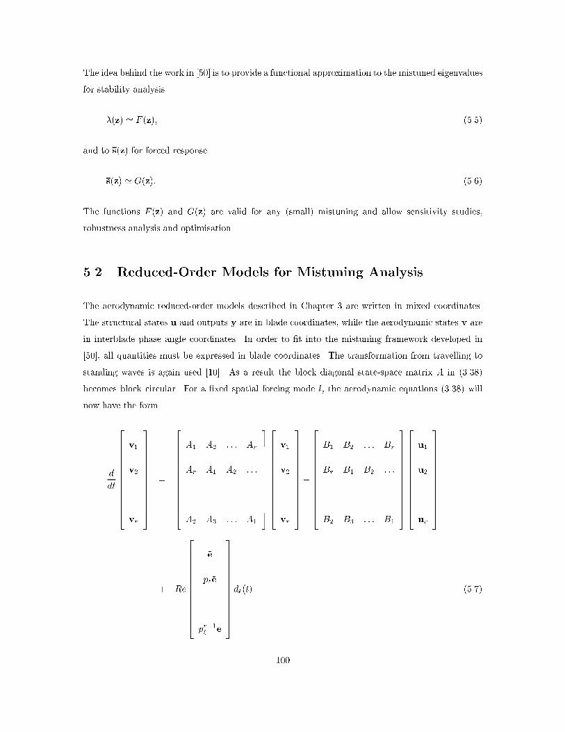
The idea behind the work in ��� is to provide a functional approximation to the mistuned eigenvalues

for stability analysis

�z � F z� ���

and to sz for forced response

sz � Gz� ���

The functions F z and Gz are valid for any small mistuning and allow sensitivity studies�

robustness analysis and optimisation�

��� Reduced�Order Models for Mistuning Analysis

The aerodynamic reduced�order models described in Chapter � are written in mixed coordinates�

The structural states u and outputs y are in blade coordinates� while the aerodynamic states v are

in interblade phase angle coordinates� In order to �t into the mistuning framework developed in

��� � all quantities must be expressed in blade coordinates� The transformation from travelling to

standing waves is again used ��� � As a result the block diagonal state�space matrix A in ����

becomes block circular� For a �xed spatial forcing mode l� the aerodynamic equations ���� will

now have the form

d

dt

��������������

v�

v�

���

vr

��������������

�

��������������

A� A� � � � Ar

Ar A� A� � � �

� � �

A� A� � � � A�

��������������

��������������

v�

v�

���

vr

��������������

�

��������������

B� B� � � � Br

Br B� B� � � �

� � �

B� B� � � � B�

��������������

��������������

u�

u�

���

ur

��������������

� Re

��������������

*e

p�*e

���

pr��� *e

��������������d�t ���

���

and ��������������

y�

y�

���

yr

��������������

�

��������������

C� C� � � � Cr

Cr C� C� � � �

� � �

C� C� � � � C�

��������������

��������������

v�

v�

���

vr

��������������� ���

where p� � e��i�r and vj now contains the aerodynamic states for blade j as opposed to states for

interblade phase angle �j�

We now consider the structural system ��� describing the plunging motion of each blade which is

written for each blade j as

&uj � Szjuj � Tyj� ���

where the structural matrix S now depends on the mistuning vector� This structural system is

coupled with the aerodynamic model ���� ��� to obtain the dynamics for blade ��

�&v�

&u�

��

�A� B�

TC� Sz�

��v�

u�

��

�A� B�

TC� �

� �v�

u�

�� �

�Ar Br

TCr �

� �vr

ur

�

� Re

�*e

�

�d�� ����

Noting that the dynamics for all other blades follow from symmetry� the complete system can be

written������������

&s�

&s�

�

�

�

&sr

������������

�

������������

M�z� M� ��� Mr

Mr M�z� M� ���

�

�

�

M� M� ��� M�zr

������������

������������

s�

s�

�

�

�

sr

������������

� Re

������������

E�

p�E�

�

�

�

pr��� E�

������������d�� ����

where

M�zi �

�A� B�

TC� Szi

�� ����

���

Mj �

�Aj Bj

TCj �

�j � �� �� � � � � r ����

and

E� �

�e

�

�� ����

Equation ���� is a special case of equation ��� and has the symmetry properties described in ��� �

��� Mistuning Analysis of Transonic Rotor

The case considered for mistuned analysis is the twenty�blade DFVLR transonic cascade discussed in

Chapter �� The blades were considered to move in unsteady plunging motion� with a tuned natural

reduced frequency chosen to be k � ������ The POD reduced�order model from section ��� was used

with �� aerodynamic states� An axial velocity defect was also admitted at the cascade inlet with

twenty possible disturbance spatial frequencies included in the model�

����� Reduced�Order Aerodynamic Model

To demonstrate the e ects of mistuning on the rotor response� structural parameters are chosen so

as to obtain a very lightly damped system� The case chosen has a blade mass ratio of � � ��� and

a structural damping of � �������� Note that a small negative value of structural damping has

been chosen� Clearly this is not physical� however it is used to establish a system which is very

lightly damped� and which therefore will exhibit a large sensitivity to mistuning� Such a mode may

actually exist in many physical systems� so it is important to determine the possible implications in

a mistuning context and to understand their sources�

For consistency with MAST analysis� time is further non�dimensionalised by t � t��kM so that the

tuned natural frequency of the blades is unity� The resulting mistuned version of equation ��� is

h��j � �� � zjh�j � � � zj

�hj � � �Cjl

�k�� ����

where the mistuning zj is a percent change in the natural frequency of blade j� The tuned structural

eigenvalues for this system are plotted in Figure ���� The frequencies fall close to the damped natural

frequency ofp

�� � � ����� The � � � structural mode is barely stable� and the � � � mode is

very lightly damped�

���

We now apply a random mistuning to the structural frequencies of the blades� generated by a normal

distribution with a zero average and a �� variance� The random mistuning pattern considered is

shown in Figure ��� along with the mistuned and tuned structural eigenvalues� It can be seen that

the lightly damped mistuned eigenvalues are to the left of the tuned ones� and so this mistuning

pattern stabilises the system� which is true for most mistuning �� � As noted in �� � the centroid of

the structural eigenvalues cannot be altered by a zero�average mistuning� In Figure ��� we see that

while the lightly damped modes are stabilised� the highly damped eigenvalues shift to the right in

order to maintain the position of the centroid� The degree of scattering of the eigenvalues about

the centroid is dependent on the amount of coupling between the aerodynamics and the structure�

Figure ��� also shows that the mistuning reduces the in�uence of the aerodynamic coupling and

moves the eigenvalues towards the centroid� as also discussed in �� �

The system is forced in the ninth nodal diameter mode � � � which corresponds to the most highly

damped tuned eigenvalue in Figure ���� The forced response is shown in Figure ��� for the tuned

case solid line and the mistuned case dotted lines� When the system is tuned� forcing in the

ninth spatial mode excites a response in only that mode� and all blades have the same response

amplitude� thus the tuned forced response is a single highly damped smooth line� When the system

is mistuned� the spatial modes no longer decouple� and forcing in the ninth spatial mode excites all

of the structural eigenvalues� including the very lightly damped � � � and � � � modes� Each blade

also now exhibits a di erent response amplitude� Because the lightly�damped modes are now present

in the response� we see sharp peaks in the mistuned Bode plot at the frequencies corresponding to

the relevant eigenvalues� Here� several blades have a large peak near � � which corresponds to

the very lightly damped � � � mode� We also see a smaller peak for one blade near � ���� which

corresponds to the � � � mode�

Although the random mistuning appears to be bene�cial in that it stabilises the system� it creates a

situation where the forced response amplitude may rise to unacceptable levels� and also introduces

high loading on some individual blades� This might create a problem in practice if a disturbance is

known to exist in a particular spatial mode whose eigenvalue is highly damped� A tuned analysis

would predict a low forced response amplitude� while in reality small blade to blade variations exist�

and the actual response may contain components of the lightly damped modes as demonstrated by

Figure ����

The idea behind robust design is to �nd an intentionally mistuned design point for the blades where

the forced response due to random mistuning will be more acceptable than that shown in Figure

���

���� The intentional mistuning is chosen so as to optimise the following objective �

Maximise +z subject to jjzjj� � ��� andX

zi � �� ����

This means that we are �nding the zero�average mistuning which provides the maximum increase in

stability � it drives the least stable eigenvalue pair as far to the left as possible� subject to a constraint

on the size of the mistuning� The optimal solution was determined in ��� and is shown in Figure

���� The corresponding eigenvalue plot shows that the least stable � � � and � � � eigenvalues have

been pushed a signi�cant amount to the left�

We now consider a random mistuning about this intentionally mistuned point� The optimal plus

random mistuning pattern is shown in Figure ��� along with the corresponding eigenvalues� Once

again� we force in the ninth spatial mode and compute the response of the tuned and mistuned

systems� The Bode plots shown in Figure ��� demonstrate that although the forced response of the

mistuned system dotted lines is higher than that of the tuned system solid line� the worst�case

amplitude has been signi�cantly reduced compared with that shown in Figure ��� for the same

random mistuning pattern� The sensitivity of the forced response to random mistuning has been

signi�cantly decreased by the introduction of intentional mistuning�

���

−0.16 −0.14 −0.12 −0.1 −0.08 −0.06 −0.04 −0.02 00.85

0.9

0.95

1

1.05

1.1

1.15

1.2

01

2 34

56

78

910

11

12

13

14

15

16

17

1819

real

imag

Figure ���� Tuned structural eigenvalues for reduced�order model� k � ������ � � ���� � ��������Eigenvalues are numbered by their nodal diameter�

���

0 2 4 6 8 10 12 14 16 18 20−0.08

−0.06

−0.04

−0.02

0

0.02

0.04

0.06

Random mistuning pattern

slot number

mis

tuni

ng

−0.16 −0.14 −0.12 −0.1 −0.08 −0.06 −0.04 −0.02 00.85

0.9

0.95

1

1.05

1.1

1.15

1.2Tuned vs Mistuned Eigenvalues

real

imag

Figure ���� Random mistuning of DFVLR rotor� Top� random mistuning pattern� Bottom� tunedeigenvalues diamonds� mistuned eigenvalues plus signs�

���

0.4 0.5 0.6 0.7 0.8 0.9 1 1.1 1.2 1.3

0

1

2

3

4

5

6

7

8

Tuned vs Mistuned Bodes

frequency

ampl

itude

|s|

Figure ���� Random mistuning of DFVLR rotor� Forced response of tuned system solid line andmistuned system dotted lines to an inlet disturbance in the ninth spatial mode�

���

0 2 4 6 8 10 12 14 16 18 20

−0.1

−0.05

0

0.05

0.1

Optimal mistuning pattern

slot number

mis

tuni

ng

−0.16 −0.14 −0.12 −0.1 −0.08 −0.06 −0.04 −0.02 00.85

0.9

0.95

1

1.05

1.1

1.15

1.2Tuned vs Mistuned Eigenvalues

real

imag

Figure ���� Optimal mistuning of DFVLR rotor� Top� optimal mistuning pattern� Bottom� tunedeigenvalues diamonds� mistuned eigenvalues plus signs�

���

0 2 4 6 8 10 12 14 16 18 20

−0.15

−0.1

−0.05

0

0.05

0.1

0.15

Optimal plus random mistuning pattern

slot number

mis

tuni

ng

−0.16 −0.14 −0.12 −0.1 −0.08 −0.06 −0.04 −0.02 00.85

0.9

0.95

1

1.05

1.1

1.15

1.2Tuned vs Mistuned Eigenvalues

real

imag

Figure ���� Optimal plus random mistuning of DFVLR rotor� Top� optimal plus random mistuningpattern� Bottom� tuned eigenvalues diamonds� mistuned eigenvalues plus signs�

���

0.7 0.8 0.9 1 1.1 1.2 1.3

0

1

2

3

4

5

6

7

8

Tuned vs Mistuned Bodes

freq w

ampl

itude

|s|

Figure ���� Optimal plus random mistuning of DFVLR rotor� Forced response of tuned systemsolid line and mistuned system dotted lines to an inlet disturbance in the ninth spatial mode�

���

����� Aerodynamic In�uence Coe�cient Model

In the analysis above� the aerodynamic forces Cjl in equation ���� are represented by the reduced�

order model which is valid over a range of frequencies and forcing inputs� Currently most analyses

use aerodynamic in�uence coe�cient models such as that described in Chapter �� The results

presented here will show that when mistuning is present� the coupling between the aerodynamics

and structural dynamics may be too large for an in�uence coe�cient model to accurately capture

the system behaviour�

An identical random mistuning pattern was applied to the in�uence coe�cient model with the same

structural parameters described above� and the eigenvalues and forced response of the system were

evaluated� Figure ��� shows the tuned and mistuned eigenvalues for the reduced�order model and

the in�uence coe�cient model� We notice that the mistuning causes the eigenvalues of the in�uence

coe�cient model to move much more than those of the reduced�order model� In Figure ��� the tuned

and mistuned eigenvalues for each model are compared� In the mistuned case� there is a greater

error in the in�uence coe�cient eigenvalues� In section ��� it was shown that the in�uence coe�cient

model does not predict the correct eigenvalue when the frequency shifts signi�cantly from the natural

frequency or when a signi�cant amount of aerodynamic damping is present� The in�uence coe�cient

model is therefore expected to provide a much worse estimate of the eigenvalues when mistuning

is present� since the interblade phase angles no longer decouple� In the tuned system� only the

aerodynamics for one interblade phase angle contribute to the placement of each eigenvalue� If a

particular mode happens to have an eigenvalue that falls close to the natural frequency with a small

amount of damping corresponding to the case of low aerodynamic coupling� then the in�uence

coe�cient model does an excellent job of predicting the eigenvalue position� This can be seen in the

top plot of Figure ��� where the eigenvalues satisfying the above requirements agree closely with the

reduced�order model� However in the mistuned system� the interblade phase angles do not decouple

and all dynamics are relevant in computing each eigenvalue� Therefore� if any modes exist whose

in�uence coe�cients are not representative for the tuned system� the eigenvalues for the mistuned

system will be inaccurate and the stability margin of the system will be mispredicted� This can be

seen in the lower plot of Figure ��� where the di erence between the reduced�order model and the

in�uence coe�cient model eigenvalues is signi�cant for all modes�

In Figure ��� the Bode plots are shown for each model in response to an inlet disturbance forcing

in the ninth spatial mode� The in�uence coe�cient model in fact does a very good job of predicting

the response� even when mistuning is present� The peak tuned response amplitude is slightly higher

than that predicted by the reduced�order model� since the tuned in�uence coe�cient eigenvalue is

���

less highly damped� The mistuned response is computed surprisingly accurately by the in�uence co�

e�cient model� despite the errors in the mistuned eigenvalue predictions� Inspection of the mistuned

eigenvalues in Figure ��� shows that the frequencies of the lightly damped � � � and � � � modes is

computed accurately� therefore the peaks of the forced response in Figure ��� occur at the correct

frequency� The damping of these two modes is predicted to be higher than it should� however this

may be compensated by the fact that the tuned � � � damping is underpredicted� thus resulting in

almost the correct forced response amplitude�

The two modes whose frequencies do move signi�cantly from the natural frequency are � � �� and

� � ��� As was shown in section ���� when this frequency shift occurs� the in�uence coe�cients

do not model the dynamics accurately� This is demonstrated by the di erence in position for the

uppermost and the lowermost eigenvalue between the reduced�order model and in�uence coe�cient

model in both plots in Figure ���� When the forced response is calculated for one of these modes� the

in�uence coe�cient model no longer predicts the amplitude accurately� Figure ���� shows the forced

response calculated for the two models for inlet disturbance forcing in the �fteenth spatial mode�

We notice �rst that the tuned forced response predictions di er� This is because the damping of the

� � �� eigenvalue is incorrectly predicted by the in�uence coe�cient calculation at the blade natural

frequency� Figure ��� shows that the damping of the eigenvalue is signi�cantly overpredicted by

the in�uence coe�cient model� which is consistent with the lower forced response amplitude� When

mistuning is introduced into the system� the in�uence coe�cient model does not capture the true

amplitudes of the peaks associated with lightly damped modes�

��� Mistuning Summary

Random mistuning is an important consideration in the design of bladed disks� since it will always

exist to some degree in practice� Although random mistuning in general stabilises the system� it

may cause a severe increase in the blade forced response amplitude� The introduction of intentional

mistuning can add su�cient damping to the lightly damped modes so that this forced response

sensitivity is reduced� The intentionally mistuned bladed disk then represents a robust design�

When a low degree of aerodynamic coupling is present in the system� the structural eigenvalues fall

close to the blade natural frequency and an aerodynamic in�uence coe�cient model can accurately

capture the dynamics� However if any signi�cant amount of coupling or a large amount of aerody�

namic damping exists� which will be true for many bladed disks in practice� these simple models

are no longer su�cient� Moreover� when mistuning is present the interblade phase angles do not

���

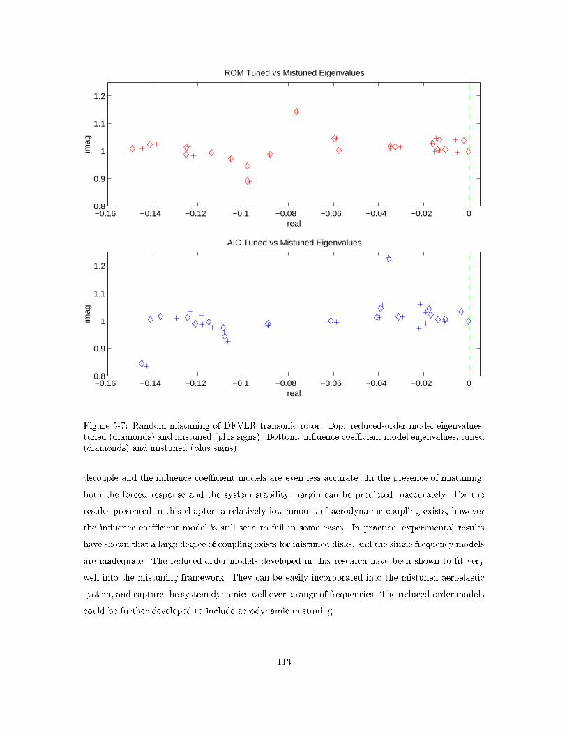
−0.16 −0.14 −0.12 −0.1 −0.08 −0.06 −0.04 −0.02 00.8

0.9

1

1.1

1.2

ROM Tuned vs Mistuned Eigenvalues

real

imag

−0.16 −0.14 −0.12 −0.1 −0.08 −0.06 −0.04 −0.02 00.8

0.9

1

1.1

1.2

AIC Tuned vs Mistuned Eigenvalues

real

imag

Figure ���� Random mistuning of DFVLR transonic rotor� Top� reduced�order model eigenvalues�tuned diamonds and mistuned plus signs� Bottom� in�uence coe�cient model eigenvalues� tuneddiamonds and mistuned plus signs�

decouple and the in�uence coe�cient models are even less accurate� In the presence of mistuning�

both the forced response and the system stability margin can be predicted inaccurately� For the

results presented in this chapter� a relatively low amount of aerodynamic coupling exists� however

the in�uence coe�cient model is still seen to fail in some cases� In practice� experimental results

have shown that a large degree of coupling exists for mistuned disks� and the single frequency models

are inadequate� The reduced�order models developed in this research have been shown to �t very

well into the mistuning framework� They can be easily incorporated into the mistuned aeroelastic

system� and capture the system dynamics well over a range of frequencies� The reduced�order models

could be further developed to include aerodynamic mistuning�

���

−0.16 −0.14 −0.12 −0.1 −0.08 −0.06 −0.04 −0.02 00.8

0.9

1

1.1

1.2

ROM vs AIC Tuned Eigenvalues

real

imag

−0.16 −0.14 −0.12 −0.1 −0.08 −0.06 −0.04 −0.02 00.8

0.9

1

1.1

1.2

ROM vs AIC Mistuned Eigenvalues

real

imag

Figure ���� Random mistuning of DFVLR transonic rotor� Top� tuned eigenvalues� reduced�ordermodel diamonds and in�uence coe�cient model plus signs� Bottom� mistuned eigenvalues�reduced�order model diamonds and in�uence coe�cient model plus signs�

���

0.4 0.6 0.8 1 1.20

1

2

3

4

5

6

7

8

9ROM Tuned vs Mistuned Bodes

freq w

ampl

itude

|s|

0.4 0.6 0.8 1 1.20

1

2

3

4

5

6

7

8

9AIC Tuned vs Mistuned Bodes

freq w

ampl

itude

|s|

Figure ���� Random mistuning of DFVLR transonic rotor� Forced response to inlet disturbance inthe � � � mode for reduced�order model left and in�uence coe�cient model right� Solid linedenotes the tuned response� dotted lines are the mistuned response�

���

0.4 0.6 0.8 1 1.20

0.5

1

1.5

2

2.5

3ROM Tuned vs Mistuned Bodes

freq w

ampl

itude

|s|

0.4 0.6 0.8 1 1.20

0.5

1

1.5

2

2.5

3AIC Tuned vs Mistuned Bodes

freq w

ampl

itude

|s|

Figure ����� Random mistuning of DFVLR transonic rotor� Forced response to inlet disturbancein the � � �� mode for reduced�order model left and in�uence coe�cient model right� Solid linedenotes the tuned response� dotted lines are the mistuned response�

���

Chapter �

Multiple Blade Row Analysis

We consider two types of blade row� In addition to the rotors described in the previous analyses�

we consider stators� or stationary blade rows� in which the blades are assumed to be rigid� The

size and nature of the reduced order models developed here lend themselves naturally to analysis of

several blade rows� State�space systems can be derived for each blade row� with sizes on the order

of ten states per blade passage� Because the models are developed in the time�domain� it is then

straightforward to couple these systems and capture inter�blade row e ects� Even with several blade

rows included in the analysis� the size of the model is small enough that unsteady simulations and

control analyses can be performed�

��� Blade Row Coupling

Adjacent blade rows will be coupled via the characteristic perturbation waves travelling between

them� Assuming subsonic axial conditions� at a passage inlet there are incoming waves in the

following three characteristic quantities

c� � p� � c���

c� � � c u�t

c� � p� � � c u�n� ���

���

which describe respectively entropy� vorticity and downstream running pressure waves� At the

passage exit� we have an upstream running pressure wave given by

c� � p� � � c u�n� ���

Note that c� � p��� c u�n at the rotor inlet is equivalent to c� at the stator exit since the character�

istics are de�ned in terms of normal vectors which always point out of the computational domain�

Here the coupling between a rotor and an upstream stator will be described� Additional blade rows

could be added in an analogous way� Consider the reduced�order model for the rotor which has

aerodynamic states vr and can be written

&vr � Arvr � Brur � E�w� � E�w� � E�w�� ���

where w�� w�� and w� are vectors containing the incoming characteristic perturbation quantities c��

c� and c� respectively at each grid point in the rotor inlet plane� These quantities are matched to

the �ow at the stator exit� and can be written in terms of the stator aerodynamic state variables vs

w�t � CrstCs�vst� w�t � CrstCs�vst� w�t � CrstCs�vst� ���

Here Csj are constant matrices depending on the mean �ow which relate the state variables vs to

the values of the characteristics at each point in the stator exit plane� For example� for a node k at

the stator exit� the kth row of Cs� contains the component of each basis vector corresponding to the

value of c� at k� Cs� and Cs� are determined similarly� using the components of the basis vectors

corresponding to c� and c� at the appropriate points� Crs is an interpolation matrix which varies

with time� and determines the �ow at the rotor inlet at a given instantaneous con�guration of the

stator�rotor combination� For example� consider the instantaneous con�guration shown in Figure

���� The value of c� at a point j in the rotor inlet plane would be contained in the jth component

of w� and could be written as a linear combination of the values of c� at the points k and k � � in

the stator exit plane� that is

cj� � �ck� � �� �ck��� � ���

where the constant � is determined from the ratio of the lengths lj�k and lj�k��� The jth row of Crs

is therefore all zeroes except for a value of � in the kth column and a value of ��� in the k� �th

column�

���

Ω

rotorinlet

stator exit

x

x

x j

k−1

k

lj,k−1

lj,k

Figure ���� Instantaneous con�guration of rotor and stator� Grid point j is in the rotor inlet plane�while points k and k � � are in the stator exit plane�

Likewise� the incoming characteristic wave at the stator exit can be written in terms of the rotor

aerodynamic state variables as follows�

w�t � CsrtCr�vrt� ���

where the matrices Csr and Cr� are de�ned in an analogous manner to those described above for

the rotor inlet� and the corresponding state�space system for the stator is

&vs � Asvs � �E�w�� ���

The stator is assumed to be rigid� so there is no forcing vector u as there is for the rotor�

The systems ��� and ��� can be combined to form a large set of equations which can be time�

marched simultaneously

�&vr

&vs

��

�Ar

�Pj��

EjCrsCsj

E�CsrCr� As

��vr

vs

��

�Brur

�

�� ���

We note that since the matrix in ��� depends on the instantaneous stator�rotor con�guration�

it varies with time� Moreover� the coe�cients of the matrix are periodic with the rotor rotation

frequency�

���

��� GE Low Speed Compressor

The multi�stage compressor analysed here is the GE low�speed research compressor which has four

repeating stages ��� � In the actual rig� each rotor has �� blades and each stator has �� vanes� In

the analysis presented here we consider a simpler case with sixteen and twenty blades in the rotor

and stator respectively� The geometry of the stage is shown in Figure ��� for a quarter of the full

wheel �ve stator blades and four rotor blades� The axial spacing between the stator and rotor is

����� of the rotor axial chord� The third stage of the compressor will be considered for analysis

here� The velocity triangles at the inlet and exits of each blade row are shown in Figure ���� Mach

numbers for the rotor are in the relative reference frame� while for the stator they are absolute�

Figure ���� Stator and rotor geometry for a single stage of the GE low�speed compressor�

���� Steady�State Solutions

The steady�state �ow for the rotor has an inlet Mach number of ����� at a �ow angle of ������ The

computed steady�state Mach contours are shown in Figure ���� Figure ��� shows the Mach contours

for the steady�state �ow through the stator� which has an inlet Mach number of ����� at an angle

of ������

���

Rotor inlet Rotor exit

Stator inlet Stator exit

0.1650.117

0.1230.089

59.3 44.7

47.3

20.2o

o

oo

Figure ���� Velocity triangles for third stage of GE low�speed compressor� Relative Mach numbersfor rotor� absolute Mach numbers for stator�

���� Unsteady Analysis

The low�speed compressor was analysed in unsteady plunging motion� Reduced�order models were

constructed for the rotor and the stator using the Arnoldi method described in Chapter �� In all

cases the Arnoldi vectors were derived about s � �� For the rotor� there are �ve relevant input

vectors� namely blade plunge displacement� blade plunge velocity and perturbations in the three

incoming inlet characteristic waves� For the stator there is just one input� which is the perturbation

in the incoming pressure wave� For the sixteen blade rotor� a total of ��� aerodynamic modes were

chosen eight modes for � � � and sixteen modes for all other interblade phase angles� For the

stator� which has twenty blades� four modes for the zero interblade phase angle and six modes for

all others were taken� for a total of ��� stator states� The coupled stator�rotor system therefore has

��� aerodynamic states�

We compare the coupled system ��� with the system for the rotor alone ���� For previous cases�

a single blade row was analysed by considering forced response time history of forces and stability

eigenvalues of the system� The crucial di erence between the coupled system ��� and the single

blade row state�space systems analysed previously is that the system matrix no longer has constant

coe�cients� For the coupled system� the interpolation matrices Crs and Csr vary with time and

are in fact periodic with the rotor rotation frequency� Rather than being �xed� each eigenvalue

���

Min: 3.8933e-02Max: 1.7493e-01

Figure ���� Mach contours for GE low�speed compressor� third stage rotor� M � ������ � � ������

of the matrix now forms a locus in the complex plane� Previously� an eigenvalue in the right half

plane indicated an unstable system� In the time�varying system� it is possible for an eigenvalue to

cross into the right half plane for part of the cycle resulting in local growth� but for the overall

system to be stable if the time spent in the right half plane is su�ciently short� The stability of the

stator�rotor system is best determined by performing time simulations�

The aerodynamic eigenvalues of the individual rotor and stator state space systems are plotted in

Figure ���� The eigenvalues of the coupled stator�rotor system at a particular time instant are

also plotted for comparison� A smaller region of this plot near the origin is shown in Figure ��

�� From Figures ��� and ���� we can see that coupling the stator has a signi�cant impact on the

aerodynamics� Although the eigenvalues of the coupled system will vary with time� the magnitude of

these variations is not expected to be very large compared with the di erences between the coupled

���

Min: 8.5789e-03Max: 1.2398e-01

Figure ���� Mach contours for GE low�speed compressor� third stage stator� M � ������ � � ������

and isolated blade row spectra�

The aerodynamic system was forced with a pulse input in plunge at one blade and all other blades

�xed� This motion excites all possible interblade phase angles in the rotor� The resulting lift forces

on each of the rotor blades were calculated using both the rotor�alone reduced�order model and the

coupled stator�rotor system� and are plotted in Figure ���� To give an indication of the time scales

on these plots� we note that the non�dimensional period for one rotor revolution is Tr � ���� The

dotted line denotes the speci�ed position of the rotor blade� the solid line is the force calculated

using the coupled model� and the dashed line is the force evaluated for the rotor alone� From Figure

��� it appears that there is a small di erence between the two force calculations� In Figure ��� the

response for just the �rst blade is plotted� which shows that the stator does have a fairly signi�cant

e ect� The magnitude of the peak response is roughly the same� but for the rotor�alone calculation�

the force on the blade dies away smoothly as the pulse passes� With the stator included in the

analysis� even after the pulse has passed through the system� we see oscillations due to the unsteady

e ect of the passing blades� These oscillations can be seen to have a period of approximately T � ���

which corresponds to one twentieth of the rotor revolution period�

���

−6 −5 −4 −3 −2 −1 0−1.5

−1

−0.5

0

0.5

1

1.5

real

imag

rotor stator rotor+stator

Figure ���� Aerodynamic eigenvalues for reduced�order models � rotor alone crosses� ��� states�stator alone plus signs� ��� states and coupled system diamonds� ��� states�

Next� a structural model for the rotor blades was coupled to the system� This model has the same

form as ���� Two structural modes per blade are added with eigenvalues near �kM� ikM � where

M is the Mach number at the rotor inlet in this case M � ������ In Figure ����� a plot of these

structural eigenvalues is shown for the rotor�alone model with structural parameters � � ���� k � ���

and � ����� For these parameters� the blade�alone eigenvalues would be at ������� ������i� For

the stator�rotor system� when the structural model ��� is coupled in� the equations take the form

���

&vr

&vs

&ur

��� �

���

Ar

�Pj��

EjCrsCsj Br

E�CsrCr� As �

TC � S

������vr

vs

ur

��� � ���

where the matrix C de�nes the forces on the rotor blades� yr � Cxr � The matrix in ��� was

evaluated at a series of time instants for the structural parameters described above� and the eigen�

values were determined� The loci of the structural eigenvalues are plotted as dots in Figure �����

The variations within the loci are small� however for some modes we notice a signi�cant di erence

between the position of the locus and the rotor�alone structural eigenvalue� For almost all modes�

���

−0.2 −0.15 −0.1 −0.05 0

−0.25

−0.2

−0.15

−0.1

−0.05

0

0.05

0.1

0.15

0.2

0.25

real

imag

rotor stator rotor+stator

Figure ���� Zoom of aerodynamic eigenvalues for rotor and stator reduced�order models�

the addition of the stator model is destabilising� which suggests that an isolated blade row analysis

could signi�cantly underpredict the response� The structural eigenvalue corresponding to � � ��

� � ������ is barely stable for the rotor�alone system� however for the coupled system its locus

lies entirely in the right half plane� We therefore have the serious case that the rotor�alone predicts

a barely stable system� but with the e ect of the stator included the system is unstable� The locus

for the unstable eigenvalue is plotted on �����

A time simulation of the coupled system was performed where an initial plunge displacement was

applied to the �rst blade� The resulting motion and force were calculated for each blade and

are plotted in Figures ���� and ���� respectively� along with the calculations for the rotor�alone

aeroelastic system� We now see some signi�cant variations between the force calculations� For all

blades� the rotor�alone model predicts a smaller response than the coupled analysis� This is consistent

with the destabilising e ect of the stator on the eigenvalues� In some cases� the rotor�alone model

predicts that the amplitude of the oscillations is barely decaying� while the coupled model predicts

a relatively rapid growth rate� due to the destabilised � � �� eigenvalue� The response for one of the

blades is plotted in Figure ���� and clearly shows the rapid increase in displacement amplitude� In

���

0 50 100−4

−2

0

2

4

blad

e 1

time0 50 100

−4

−2

0

2

4

blad

e 2

time0 50 100

−4

−2

0

2

4

blad

e 3

time0 50 100

−4

−2

0

2

4

blad

e 4

time

0 50 100−4

−2

0

2

4

blad

e 5

time0 50 100

−4

−2

0

2

4

blad

e 6

time0 50 100

−4

−2

0

2

4

blad

e 7

time0 50 100

−4

−2

0

2

4

blad

e 8

time

0 50 100−4

−2

0

2

4

blad

e 9

time0 50 100

−4

−2

0

2

4

blad

e 10

time0 50 100

−4

−2

0

2

4

blad

e 11

time0 50 100

−4

−2

0

2

4

blad

e 12

time

0 50 100−4

−2

0

2

4

blad

e 13

time0 50 100

−4

−2

0

2

4

blad

e 14

time0 50 100

−4

−2

0

2

4

blad

e 15

time0 50 100

−4

−2

0

2

4

blad

e 16

time

Figure ���� Aerodynamic response to pulse displacement input at blade �� Blade plunge displacementprescribed� dotted line� rotor alone blade vertical force dashed line and rotor�stator system bladevertical force solid line�

this example� the stator clearly has an important in�uence and should be included in an aeroelastic

analysis�

��� Summary

A low�order aeroelastic model has been derived for two blade rows in a subsonic compressor� The

model has less than four hundred aerodynamic states� which is reasonable for time marching sim�

ulations and the evaluation of eigenvalues� Stability cannot be de�ned in the same way as for the

rotor�alone model by computing the system eigenvalues� since the coe�cient matrix varies with time�

However� the eigenvalues of the matrix can be computed at various time instants over the rotor rev�

olution period� and loci determined for the eigenvalues� A time simulation can also be performed

���

0 20 40 60 80 100 120−1

−0.8

−0.6

−0.4

−0.2

0

0.2

0.4

0.6

blad

e 1

forc

e

time

rotor rotor+stator

Figure ���� Aerodynamic response of blade � to pulse displacement input at blade �� Rotor�alonemodel dashed line and rotor�stator coupled model solid line�

by applying an initial perturbation to the rotor� The stability of the system can be characterised by

considering the resulting aeroelastic response�

For the case presented here� inter�blade row e ects are shown to be very signi�cant� For most modes�

the addition of the upstream stator has a destabilising e ect� As a result� the response amplitude

of the coupled stator�rotor aeroelastic system is much larger than that predicted by the isolated

rotor analysis� The degree of inter�blade row coupling will vary between problems� depending on

the �ow conditions and the distance between adjacent blade rows� The model developed in this

chapter provides a means of quantifying the e ect� For a given problem� preliminary analysis can be

performed to determine whether deriving models for an isolated blade row is su�cient� or whether

upstream and downstream blade rows should be included to accurately capture the system dynamics�

If the addition of an upstream blade row is destabilising� as in the example presented here� it is

especially important that it is included in the analysis� Moreover� if viscous e ects were included in

���

−20 −15 −10 −5 0

x 10−3

0.08

0.082

0.084

0.086

0.088

0.09

1

13

14

2

12

16 11 3 10

9

6 5

4 15 8

7

Figure ����� Structural eigenvalues � rotor�alone system crosses and periodic loci for coupledstator�rotor model dots� Eigenvalues are numbered by their nodal diameter �� � � ������ � ���� k � ���� � �����

the model� we would expect the in�uence of the upstream blade row to be even greater due to the

presence of the viscous wakes� We might also expect a transonic stage� where shocks are present�

to exhibit a higher degree of inter�blade row coupling� The amount of in�uence seen here for an

inviscid� low subsonic stage suggests that in general� inter�blade row e ects are very important and

should be included in aeroelastic analyses�

���

1.1 1.2 1.3 1.4 1.5 1.6 1.7 1.8 1.9 2

x 10−3

0.0806

0.0808

0.081

0.0812

0.0814

0.0816

0.0818

Figure ����� Periodic locus of structural eigenvalue for � � �� mode�

���

0 100 200 300

−1

0

1

blad

e 1

time0 100 200 300

−1

0

1bl

ade

2

time0 100 200 300

−1

0

1

blad

e 3

time0 100 200 300

−1

0

1

blad

e 4

time

0 100 200 300

−1

0

1

blad

e 5

time0 100 200 300

−1

0

1

blad

e 6

time0 100 200 300

−1

0

1

blad

e 7

time0 100 200 300

−1

0

1

blad

e 8

time

0 100 200 300

−1

0

1

blad

e 9

time0 100 200 300

−1

0

1

blad

e 10

time0 100 200 300

−1

0

1

blad

e 11

time0 100 200 300

−1

0

1

blad

e 12

time

0 100 200 300

−1

0

1

blad

e 13

time0 100 200 300

−1

0

1

blad

e 14

time0 100 200 300

−1

0

1

blad

e 15

time0 100 200 300

−1

0

1

blad

e 16

time

Figure ����� Response due to an initial plunge displacement at blade �� Blade displacement calcu�lated with rotor�alone model dashed lines and coupled stator�rotor model solid lines� � � ����k � ���� � �����

���

0 100 200 300

−2

0

2

blad

e 1

time0 100 200 300

−2

0

2bl

ade

2

time0 100 200 300

−2

0

2

blad

e 3

time0 100 200 300

−2

0

2

blad

e 4

time

0 100 200 300

−2

0

2

blad

e 5

time0 100 200 300

−2

0

2

blad

e 6

time0 100 200 300

−2

0

2

blad

e 7

time0 100 200 300

−2

0

2

blad

e 8

time

0 100 200 300

−2

0

2

blad

e 9

time0 100 200 300

−2

0

2

blad

e 10

time0 100 200 300

−2

0

2

blad

e 11

time0 100 200 300

−2

0

2

blad

e 12

time

0 100 200 300

−2

0

2

blad

e 13

time0 100 200 300

−2

0

2

blad

e 14

time0 100 200 300

−2

0

2

blad

e 15

time0 100 200 300

−2

0

2

blad

e 16

time

Figure ����� Response due to an initial plunge displacement at blade �� Blade force calculated withrotor�alone model dashed lines and coupled stator�rotor model solid lines� � � ���� k � ���� � �����

���

0 50 100 150 200 250 300−0.2

−0.1

0

0.1

0.2

time

blad

e 13

dis

plac

emen

t

0 50 100 150 200 250 300−4

−2

0

2

4

time

blad

e 13

forc

e

rotor rotor+stator

Figure ����� Response due to an initial plunge displacement at blade �� Displacement and forceon the thirteenth blade calculated with rotor�alone model dashed lines and coupled stator�rotormodel solid lines� � � ���� k � ���� � �����

���

Chapter �

Conclusions and Recommendations

The aeroelastic model can be formulated as an input�output problem� where the challenge is to

�nd a means of accurately representing the aerodynamics and the structural dynamics� and the

interaction between the two� Although CFD and �nite element methods may provide models with

the desired level of accuracy� they are high order and are therefore not suitable for design or control

analysis� Moreover� because the number of controlling parameters in the aerodynamic framework

is very high� CFD approaches are generally too expensive for routine determination of stability

boundaries� Low�order aerodynamic models can be obtained by systematic reduction of a high�order

CFD method� The resulting models replicate the output behaviour of the high��delity CFD method

over a restricted range of inputs� The reduction can be performed according to the speci�c problem

and which dynamics are considered important� yielding models for a wide range of applications�

Reduced�order aerodynamic models have been developed for the unsteady� linearised� two�dimensional

Euler equations� Model order reduction has been demonstrated for both subsonic and transonic blade

rows operating in unsteady plunging motion� and shows that three orders of magnitude reduction

from the original CFD model is possible� while still accurately capturing the dynamics relevant to

�utter and forced response� Simple assumed�frequency aerodynamic models are also derived using

the high�order CFD method� These models are of the kind currently used in many aeroelastic anal�

yses� and provide high��delity� low�order aerodynamics� but are strictly only valid at the assumed

conditions� It is shown that for typical turbomachinery problems� a high degree of coupling exists

between the �ow and the structure� and in many situations these simple models inaccurately pre�

dict the system aeroelastic response� Derivation of reduced�order models using the Arnoldi�based

approach is of comparable expense to the assumed�frequency method� but can accurately model

���

aeroelastic response for a range of inputs�

The reduced�order models are developed in the time domain for the full blade row for several reasons�

Firstly� state�space form makes them appropriate for control applications and also allows them to

be easily coupled to models of other engine components� To demonstrate this coupling� a model is

constructed for a low�speed compressor stage with a stator�rotor con�guration� The reduced�order

model has less than four hundred states for the coupled stator�rotor system� which allows forced

response and stability of the stage to be assessed� The results show that the stator may have an

important destabilising e ect on the rotor dynamics� and should be included in the analysis if the

aeroelastic properties are to be predicted accurately� Secondly� because the models are developed

for the full rotor� they can be applied to problems which lack cyclic symmetry� Blade mistuning has

been identi�ed as an important factor in determining aeroelastic response� however to date there has

been a lack of high��delity aerodynamic models suitable for incorporation to a mistuning framework�

Current analyses use assumed�frequency models which are even more inadequate when mistuning

is present� The reduced�order models developed in this thesis couple naturally into a mistuned

analysis� and have been used to investigate structural mistuning in a transonic rotor�

There are a number of extensions which could be applied to the reduced�order models developed

in this research� These extensions include improvements on the model order reduction technique

and possibilities for additional model applications� It is important to note that although two�

dimensional� inviscid �ows were considered here� the methodology applies to any linearised CFD

model� If this underlying CFD code were available� it would be straightforward to consider three�

dimensional and�or viscous e ects� Inclusion of these e ects would allow analysis of interesting

�ow phenomena such as tip clearance leakage �ows� secondary �ows in the blade passages and

rotating stall� Moreover� since the Arnoldi vectors approximate the eigenvectors� investigation of

the eigenmodes of the reduced�space basis can provide useful physical insight�

In terms of methodology� the Arnoldi�based approach has been used successfully to derive accurate

low�order models very e�ciently� This method provides several interesting options for future re�

search� In this work� models were derived using a McLaurin expansion of the transfer function� An

interesting extension would be to perform the expansion about some non�zero frequency point� A

natural choice might be the blade natural frequency� due to the nature of the aeroelastic system� the

blade response comprises a range of frequencies about this point� While a single frequency model

cannot span this range accurately� an Arnoldi reduced�order model with just a few states could very

accurately capture the important dynamics� with just a small increase in computational cost� In

addition� the Arnoldi models presented here were derived by considering inputs of interest� It would

���

also be possible to consider outputs of interest by formulating the dual problem� If the number of

inputs exceeds the number of outputs� this approach would be computationally more e�cient� To

obtain an improved model� a balanced realisation could also be implemented� in which both inputs

and outputs of interest are considered�

There are many applications within a turbomachinery context to which one could envision imple�

menting these models� In many cases� current analysis and design tools utilise very simple aero�

dynamic models which are often insu�cient� Due to the general time�domain� input�output form

chosen� the reduced�order models developed here can be easily incorporated into virtually any frame�

work� For example� the time domain approach provides a convenient framework for incorporating the

compressor analysis within a global engine model� such as the Moore�Greitzer model� In this model�

the blade row is represented simply as an actuator disk� but could be replaced with a reduced�order

model with appropriate boundary conditions� This framework would allow an accurate analysis of

inlet distortions and surge� The use of generalised boundary conditions also allows the high��delity

aerodynamics to be incorporated within other frameworks� such as analysis of acoustical interactions�

A particular application in which a serious need for suitable higher �delity aerodynamic models has

been identi�ed is mistuning� Reduced�order models have been used in this research to demonstrate

the e ects of structural mistuning in a rotor� Signi�cant interest also exists in the e ects of aero�

dynamic mistuning� Within the linearised framework described here� sensitivities to blade shape

and incidence could be included in the model� Thus the e ects of aerodynamic mistuning could be

investigated� both in an analysis and a design context�

The major restriction of the reduced�order models developed in this thesis is the assumption of

small perturbation unsteady �ow� In some cases nonlinear e ects may be important� for example

in unsteady transonic �ows the motion of shocks may have a large nonlinear e ect on the solution�

Limit cycling is another nonlinear phenomenon exhibited by unsteady �ows and is important if

�utter stability boundaries are to be predicted accurately� Some consideration needs to be given to

incorporating nonlinear e ects into the models� It is possible to envision snapshots for a POD model

being obtained from a full nonlinear simulation� Such a simulation would need to be performed in the

time domain on the full rotor for each frequency and Mach number of interest� thus the computational

cost would be signi�cantly increased�

It is clear that reduced�order aerodynamic modelling o ers a huge potential for improvement in

aeroelastic analysis and design tools� The framework utilised is very general� enabling incorporation

of the models to many di erent applications� The research has developed a methodology for obtaining

such models e�ciently in a turbomachinery context� and identi�ed several possible applications�

���

Appendix A

GMRES Algorithm

The solution of a large linear system can be performed e�ciently through use of a generalised

minimal residual algorithm GMRES ��� �

The algorithm is best described by considering a di erentiable system expressed in vector form as

F U � �� A��

Given an approximate solution Un� we construct k orthonormal search directions� pj � as follows�

p� �F Un

jjF Unjj � A��

For j � �� �� ���k � � take

%pj� � F Un� pj�jX

i��

bijpi A��

and set

pj� �%pj�jj%pj�jj � A��

where

bij � F Un� pj�pi A��

and F Un� pj denotes the directional derivative of F evaluated at Un in the direction of pj and is

���

approximated as

F Un� pj F Un � �pj� F Un

�� A��

where � is taken to be a small number proportional to jjUnjj�

Once the k search directions are known� Un is updated according to

Un� � Un �kX

j��

ajpj � A��

where the coe�cients aj are evaluated by minimising jjF Un�jj�� The performance of this algo�

rithm is very dependent on the use of a suitable preconditioner� In this research an incomplete LU

factorisation routine from the SPARSKIT library ��� was used�

���

Bibliography

�� Bolcs A� and T�H� Fransson� Aeroelasticity in Turbomachines� Comparison of Theoretical

and Experimental Cascade Results� Technical Report AFOSR�TR�������� Ecole Polytechnique

Federale de Lausanne� �����

�� J�J� Adamczyk and M�E� Goldstein� Unsteady Flow in a Supersonic Cascade wuth Subsonic

Leading�Edge Locus� AIAA Journal� ���������,����� September �����

�� O�O� Bendiksen� Flutter of Mistuned Turbomachinery Rotors� ASME ���GT����� �����

�� G� Berkooz� P� Holmes� and J�L� Lumley� The Proper Orthogonal Decomposition in the Analysis

of Turbulent Flows� Annual Review of Fluid Mechanics� ������,���� �����

�� R�L� Bisplingho and H� Ashley� Principles of Aeroelasticity� Dover Publications� New York�

NY� �����

�� D�H� Bu um� Blade Row Interaction E ects on Flutter and Forced Response� AIAA Paper

�������� �����

�� E�F� Crawley� Aeroelastic Formulation for Tuned and Mistuned Rotors� AGARD Manual on

Aeroelasticity in Axial�Flow Turbomachines� Volume �� �����

�� E�F� Crawley and K�C� Hall� Optimization and mechanisms of mistuning in cascades� Trans�

actions of the ASME� �������,���� April �����

�� E�H� Dowell� K�C� Hall� J�P� Thomas� R� Florea� B�I� Epureanu� and J� Heeg� Reduced Order

Models in Unsteady Aerodynamics� AIAA Paper �������� �����

��� J� Dugundji and D�J� Bundas� Flutter and Forced Response of Mistuned Rotors Using Standing

Wave Analysis� AIAA Journal� ���������,����� November �����

��� R�C�F� Dye and T�A� Henry� Vibration Amplitudes of Compressor Blades Resulting from Scatter

in Blade Natural Frequencies� ASME Journal of Engineering for Power� ������,���� July �����

���

��� D�J� Ewins� The E ects of Detuning Upon the Forced Vibrations of Bladed Disks� Journal of

Sound and Vibration� �����,��� �����

��� P� Feldmann and R�W� Freund� E�cient Linear Circuit Analysis by Pad!e Approximation via

the Lanczos Process� IEEE Transactions on Computer�Aided Design of Integrated Circuits and

Systems� ������,���� �����

��� R� Florea� K�C� Hall� and P�G�A� Cizmas� Reduced Order Modelling of Unsteady Viscous Flow

in a Compressor Cascade� AIAA Paper �������� �����

��� M�B� Giles� Non�Re�ecting Boundary Conditions for the Euler Equations� CFDL�TR �����

Massachusetts Institute of Technology� February �����

��� M�B� Giles� Stator�Rotor Interaction in a Transonic Turbine� Journal of Propulsion and Power�

������,���� �����

��� M�B� Giles and R� Haimes� Validation of a Numerical Method for Unsteady Flow Calculations�

ASME International Gas Turbine and Aeroengine Congress and Exposition� Paper ���GT�����

Orlando� Florida� �����

��� W�R� Graham� J� Peraire� and K�Y� Tang� Optimal Control of Vortex Shedding Using Low�

Order Models� Part II � Model�Based Control� International Journal for Numerical Methods in

Engineering� ������,���� �����

��� E� Grimme� Krylov Projection Methods for Model Reduction� PhD thesis� Coordinated�Science

Laboratory� University of Illinois at Urbana�Champaign� �����

��� K� C� Hall� J� P� Thomas� and E� H� Dowell� Reduced�Order Modelling of Unsteady Small�

Disturbance Flows Using a Frequency�Domain Proper Orthogonal Decomposition Technique�

AIAA Paper �������� �����

��� K�C� Hall� A Linearized Euler Analysis of Unsteady Flows in Turbomachinery� PhD thesis�

Dept� of Aeronautics and Astronautics� MIT� May �����

��� K�C� Hall� Eigenanalysis of Unsteady Flows About Airfoils� Cascades and Wings� AIAA

Journal� ���������,����� December �����

��� K�C� Hall and E�F� Crawley� Calculation of Unsteady Flows in Turbomachinery Using the

Linearized Euler Equations� AIAA Journal� �������,���� September �����

��� K�C� Hall� R� Florea� and P�J� Lanzkron� A Reduced Order Model of Unsteady Flows in

Turbomachinery� ASME Paper ���GT����� �����

���

��� K�C� Hall and P�D� Silkowski� The In�uence of Neighboring Blade Rows on the Unsteady

Aerodynamic Response of Cascades� ASME ���GT���� �����

��� D�E� Hobbs� J�H� Wagner� J�F� Dannenho er� and R�P� Dring� Supercritical Airfoil Technology

Program� Wake Experiments and Modeling for Fore and Aft�Loaded Compressor Cascades�

Final Report FR������� Pratt and Whitney Aircraft Group� UTC� September �����

��� M� Kamon� F� Wang� and J�K� White� Recent Improvements to Fast Inductance Extraction

and Simulation� Proceedings of the �th Topical Meeting on Electrical Performance of Electronic

Packaging� West Point� NY� October �����

��� K�R� Kaza and R�E� Kielb� Coupled Bending�Torsion Flutter of a Mistuned Cascade with

Nonuniform Blades� AIAA Paper �������� �����

��� K�R� Kaza and R�E� Kielb� Flutter and Response of a Mistuned Cascade in Incompressible

Flow� AIAA Journal� ��������,����� August �����

��� J� Kenyon and D� Rabe� Aerodynamic E ects on Blade Vibratory Stress Vibrations� AIAA

Paper �������� Lake Buena Vista� Florida� �����

��� J�L� Kerrebrock� Aircraft Engines and Gas Turbines� MIT Press� Cambridge� �nd edition� �����

��� T� Kim� Frequency�Domain Karhunen�Loeve Method and Its Application to Linear Dynamic

Systems� AIAA Journal� ���������,����� �����

��� M� Kruse and C� Pierre� Dynamic Response of an Industrial Turbomachinery Rotor� Proceedings

of the ��nd AIAA�ASME�SAE�ASEE Joint Propulsion Conference and Exhibit� �����

��� M� Kruse and C� Pierre� Forced Response of Mistuned Bladed Disks using Reduced�Order

Modeling� AIAA Paper ��������CP� �����

��� R�B� Lehoucq� D�C� Sorensen� and C� Yang� ARPACK Users Guide� Solution of Large Scale

Eigenvalue Problems by Implicitly Restarted Arnoldi Methods� Rice University� October �����

��� M� Lo!eve� Probability Theory� D� Van Nostrand Company Inc�� New York� �����

��� J�L� Lumley� The Structures of Inhomogeneous Turbulent Flow� Atmospheric Turbulence and

Radio Wave Propagation� pages ���,���� �����

��� A�J� Mahajan� E�H� Dowell� and D�B� Bliss� Eigenvalue Calculation Procedure for an

Euler�Navier�Stokes Solver with Application to Flows over Airfoils� Journal of Computational

Physics� ������,���� �����

���

��� S�R� Manwaring and D�C� Wisler� Unsteady Aerodynamics and Gust Response in Compressors

and Turbines� Journal of Turbomachinery� ��������,���� �����

��� F�K� Moore and E�M� Greitzer� A Theory of Post�Stall Transients in Axial Compression Sys�

tems� Part I � Development of Equations� Journal of Engineering for Gas Turbines and Power�

������,��� January �����

��� B�R� Noack and H� Eckelmann� A global stability analysis of the steady and periodic cylinder

wake� Journal of Fluid Mechanics� �������,���� �����

��� G�S� Ottarsson� M�P� Castanier� and C� Pierre� A Reduced�Order Modeling Technique for

Mistuned Bladed Disks� Proceedings of the ��th AIAA�ASME�ASCE�AHS�ASC Structures�

Structural Dynamics� and Materials Conference� �����

��� G�S� Ottarsson and C� Pierre� On the E ects of Interblade Coupling on the Statistics of

Maximum Forced Response Amplitudes in Mistuned Bladed Disks� Proceedings of the ��th

AIAA�ASME Structures� Structural Dynamics� and Materials Conference� �����

��� M�M� Rai� Navier�Stokes Simulations of Rotor�Stator Interaction Using Patched and Overlaid

Grids� Journal of Propulsion and Power� ������,���� �����

��� M�C� Romanowski� Reduced Order Unsteady Aerodynamic and Aeroelastic Models using

Karhunen�Lo!eve Eigenmodes� AIAA Paper ������� �����

��� M�C� Romanowski and E�H� Dowell� Using Eigenmodes to Form an E�cient Euler Based

Unsteady Aerodynamics Analysis� Proceedings of the Special Symposium on Aeroelasticity and

Fluid�Structure Interaction Problems� ASME International Mechanical Engineering Congress

and Exposition� AD�Vol� ��� pp� �������� �����

��� Y� Saad� Numerical Methods for Large Eigenvalue Problems� Manchester University Press

Series in Algorithms and Architectures for Advanced Scienti�c Computing� �����

��� Y� Saad� SPARSKIT� a basic tool kit for sparse matrix computations� Version � User Manual�

June �����

��� B� Shapiro� Symmetry Approach to Extension of Flutter Boundaries via Mistuning� Journal of

Propulsion and Power� �������,���� May�June �����

��� B� Shapiro� Passive Control of Flutter and Forced Response in Bladed Disks via Mistuning�

PhD thesis� California Institute of Technology� May �����

���

��� P�D� Silkowski� Measurements of Rotor Stalling in a Matched and Mismatched Compressor�

GTL Report ���� MIT� April �����

��� L�M� Silveira� M� Kamon� I� Elfadel� and J� White� A Coordinate�Transformed Arnoldi Algo�

rithm for Generating Guaranteed Stable Reduced�Order Models of RLC Circuits� Computer

Methods in Applied Mechanics and Engineering� ����������,���� February �����

��� L� Sirovich� Turbulence and the Dynamics of Coherent Structures� Part � � Coherent Structures�

Quarterly of Applied Mathematics� �������,���� October �����

��� T� Theodorsen� General Theory of Aerodynamic Instability and the Mechanism of Flutter�

Report ���� NACA� �����

��� L�N� Trefethen and D� Bau� Numerical Linear Algebra� SIAM� Philadelphia� PA� �����

��� J�M� Verdon� Review of Unsteady Aerodynamic Methods for Turbomachinery Aeroelastic and

Aeroacoustic Applications� AIAA Journal� �������,���� February �����

��� S�T� Wei and C� Pierre� Localization Phenomena in Mistuned Assemblies with Cyclic Symmetry�

Part I� Free Vibrations� ASME Journal of Vibration� Acoustics� Stress� and Reliability in Design�

��������,���� �����

��� S�T� Wei and C� Pierre� Localization Phenomena in Mistuned Assemblies with Cyclic Symmetry�

Part II� Forced Vibrations� ASME Journal of Vibration� Acoustics� Stress� and Reliability in

Design� ��������,���� �����

��� D�S� Whitehead� Vibration of Cascade Blades Treated by Actuator Disc Methods� Proceedings

of the Institution of Mechanical Engineers� ���������,���� �����

��� D�S� Whitehead� Force and Moment Coe�cients for Vibrating Airfoils in Cascade� British

Aeronautical Research Council� London� R�-M� ����� February �����

��� D�S� Whitehead� Classical Two�Dimensional Methods� AGARD Manual on Aeroelasticity in

Axial�Flow Turbomachines� Unsteady Turbomachinery Aerodynamics� Volume �� �����

��� L�B� Wigton� N�J� Yu� and D�P� Young� GMRES Acceleration of Computational Fluid Dynamics

Codes� AIAA Paper �������� �����

��� Karen E� Willcox� Aeroelastic Computations in the Time Domain Using Unstructured Meshes�

Master�s thesis� Dept� of Aeronautics and Astronautics� MIT� February �����

���

��� K�E� Willcox� J�D� Paduano� J� Peraire� and K�C� Hall� Low Order Aerodynamic Models for

Aeroelastic Control of Turbomachines� AIAA Paper �������� �����

��� K�E� Willcox� J� Peraire� and J� White� An Arnoldi Approach for Generation of Reduced�Order

Models for Turbomachinery� Submitted� Computers and Fluids� �����

���