Poverty Incidence,Infrastructure Development and

Human Capital: an Empirical StudyOf Provinces in the Philippines

Edgardo Manuel Miguel M. JopsonDe La Salle University – ManilaEmail: manuel.jopson@gmail.com / edgardo_jopson@dlsu.ph Cellular number: (+63) 916 464 4412

Abstract:

Current literature in economic development emphasizes the impact of investing in infrastructure and human

capital. In the Philippines with its provinces’ different economic situations, a generalized policy recommendation

can yield problematic results. Using data gathered from the National Statistics Office (NSO), the Department of

Public Works and Highways (DPWH), as well as the National Statistical Coordination Board (NSCB) from 2009,

and employing Ordinary Least Squares estimation procedure, the study aims to present the possible relationships

between poverty and specific factors of economic development, such as the valuation of buildings, roads,

educational attainment and population growth. This study may be of contribution by providing a clearer picture on

the rural economic situation of the Philippines and aid policymakers in decision making.

JEL Classification: O15, O18, O40

Keywords: Poverty, infrastructure, human capital, rural economic development, Philippines

1. Introduction

1.1 Background of the Study

The problem of poverty is far from being

eradicated in most developing countries. In the

Philippines alone in 2012, there is an estimated

22.9% of the population of the country is considered

poor, with the Autonomous Region of Muslim

Mindanao having the highest level of poverty

incidence at 46.9% (National Statistical Coordination

Board, 2013). To meet the Millennium Development

Goal of the United Nations of eradicating extreme

poverty, the Philippines must address this problem in

the most efficient way that it can.

In a study made by the Asian Development Bank

in 2007 the critical constraints to poverty reduction

are access to economic opportunities (lack and slow

growth of productive employment and opportunities),

human development (access to primary and

secondary education and health service), access to

basic social services and productive assets (basic

infrastructure, poor’s limited access to financing and

land) and the lack on the coverage of social safety

nets (ADB, 2007: 41-48). These problems are indeed

faced by mostly the Filipino lower class, and until

today still are so. By studying the economic situation

of the Philippines in a broader perspective that

encompasses not just physical and material outputs

but includes health, wellness, education, political

situations, among others in relation to the

infrastructure development, employment, and

investments - it would be possible to find appropriate

solutions to the problem of poverty.

According to the Asian Development Bank, the

main causes of poverty in the country are the

following:

a. Low to moderate economic growth for

the past 40 years;

b. Low growth elasticity of poverty

reduction;

c. Weakness in employment generated and

the quality of jobs generated;

d. Failure to fully develop the agricultural

sector;

e. High inflation during crisis periods;

f. High levels of population growth;

g. High and persistent levels of inequality

(income and assets) which dampen the

positive impacts of economic

expansion; and

h. Recurrent shocks and exposure to risks

as economic crisis, conflicts, natural

disasters, and “environmental poverty”

(ADB, 2009: 2)

The Philippines is currently a developing

economy that is beginning to make its presence felt in

the international market, with a quarterly gross

domestic product growth for the year 2012 rate as

follows: 6.3%, 6.0%, 7.2% and 6.8%. However, in

2011 the Philippines still ranks 112 out of 187

countries in terms of its Human Development Index

or HDI at 0.627 (UNDP, 2011). Functional literacy

rate is still at 84.1%, with 81.9% for males and

86.3% for females in 2003. In the year 2006 life

expectancy for females and males were 72.5% and

67.8%. GDP per capita for both current and 1985

prices are at 68,989 and 14,653 respectively. What do

these numbers represent? Functional literacy rate, life

expectancy, primary and secondary enrolment rate

and GDP per capita are the components for the

computation of HDI, which is used as a yardstick for

measuring the quality of living of a group of people,

and from merely inspecting these numbers, it is

possible to infer that the Philippines is in need of

increasing its HDI.

Infrastructure development is an integral part of

economic development, as it is one of the key

indicators for growth in an economy. Building

infrastructure not only provides employment with

regard to the initial construction, but provides the

community an overall positive benefit from it;

creating roads and bridges make transportation of

goods and services easier, more efficient and less

costly. Buildings create space for commerce,

government and housing, water pipelines and

sewerage systems provide households, businesses

and government buildings clean water and hygienic

disposal of human waste and dirt, parks and other

recreational areas provide additional income for the

economy from both foreign and local tourism leading

to an increase of commercial establishments, an

increase of employment and an overall increase of

the economy’s GDP. Infrastructures give way to a

multitude of human activities just waiting to be

established.

2

Capital deepening is a vital concept in capital

theory. Given a steady state Economy with one kind

of capital good, capital deepening is defined as the

case wherein the per worker capital good stock is a

decreasing function of its own rate of interest . In

Neo-classical macroeconomics which focuses on

capital accumulation and its links to saving decisions,

the marginal condition f ' (k )=price and the rate of

return ( r+δ=f ' (k )) where r is the principal rate of

return and δ is the rate of depreciation, lead to a per

capital return that is higher than before (Hirota,

1979), which can be done by providing more

employment in the economy as well as increasing its

capital (McEachern, 2012). Take for example the

province of Catanduanes, barely featured in mass

media, literature and politics, it is the easternmost

province in the Bicol region. However according to

the NSCB Catanduanes is the top Bicol province in

HDI, ranking 21st among the provinces of the country

(National Statistical Coordination Board, 2013), and

when we consider its human capital we can find some

interesting data. In 2011’s Civil Engineering Board

Exam, the top 1, 2 and 3 are from the Catanduanes

State Colleges, and obtained a passing rate of

69.84%- well above the national mean of 34.28% and

has consistently had civil engineering board

examination top passers since (GSRubio/PR and

Information Services, 2013); for the Board Exam for

Nurses has had an 85% passing rate in 2009, and in

2007 ranked 45 of all provinces in the Philippines;

and in the Licensure Examination for Teachers in the

elementary level in 2007 has ranked 40 of all

provinces with a passing rate of 42% (National

Statistical Coordination Board, 2007). However the

province’s income generating activities in

comparison to other provinces in the same region

such as Camarines Sur, such as tourism, is less.

Although Catanduanes is an internationally known

surfing spot, it still draws significantly less tourists

than Camarines Sur, due to it being a kept secret

among pro surfers (Puraran Surf Beach Resort,

2013). According to the Provincial Framework and

Physical Development Plan (PDPF) of Catanduanes,

although the growth rate of the travellers to

Catanduanes has shot up to 198% from 2008 to 2009,

Camarines Sur has still hauled in 38,385 foreign

tourists and 147,758 domestic tourists- significantly

less than Catanduanes’ 8,984 foreign tourists and

36,722 domestic tourists; hence indicated in the

PDPF are policies to increase their revenues in

tourism by investing in eco-tourism. In comparison to

Camarines Sur’s performance, Catanduanes has

shown improvement as a rural province which can be

seen from its academic performance as well as its

significant spike in tourism.

1.2 Statement of the Problem

In the Philippines where the population of the

poor and oppressed greatly outnumber the elite and

powerful, it has become more difficult to determine

key indicators in terms of the quality of life of every

individual, even more difficult to make sound

decisions when it comes to finding solutions to

alleviate poverty by maximizing the limited resources

the country has. This study determines the

significance of capital deepening and infrastructure

development with respect to poverty incidence,

which pertains to policies that may be made in terms

of allocation of resources to particular sectors of the

economy that will be at most opportunity cost-

minimizing and maximizing its effect to benefit

society.

1.3 Objectives

3

This research paper intends to:

1. Present an econometric model that would

allow the proponent to determine the

relationship of poverty via the poverty

incidence with infrastructure development

and capital deepening and make relevant and

statistically sound conclusions;

2. Describe the effect of an expansionary fiscal

policy via an increase in government

spending, with regards to creation of new

roads, developing human capital e.g.

providing scholarships and training

(additional school years), and its

significance to the well-being of society that

will be determined by the significance of the

relationship of poverty with infrastructure

development and human capital

development;

3. Provide a supplementary aide to policy

makers and make sound recommendations

from the regression analysis generated from

the econometric method.

1.4 Significance of the Study

The study attempts to determine whether or not

there is a significant link on infrastructure

development and capital deepening to the poverty

incidence of the country. It can serve as a

contribution to the field of rural development in the

Philippines in the continuous efforts of the county to

attain its macroeconomic goals to sustainable

economic growth and development. It may also aide

policymakers in the rural areas in the country in

creating sound economic decisions and policies as

well as future projects that may benefit their

respective communities and how it may affect the

well-being of every individual. The paper can also be

attributed to the United Nation’s Millennium

Development Goals in developing a global

partnership for development and for eradicating

extreme poverty, which is for the improvement of the

quality of living of the people of the economy.

1.5 Scope and Limitations

The method used in this study uses the Ordinary

Least Squares estimation method1 and is limited to a

cross-section analysis, which might not perfectly

capture reality, however does not mean that it should

be considered insignificant altogether. The data used

in this research will be drawn from the databases of

the National Statistical Coordination Board, NSO,

and DPWH. This study will also include

infrastructure development and capital Deepening

determinants such as the value of new constructions,

population and number of households with access to

water, as well as the average years of schooling.

2. Review of Related Literature

2.1 Poverty Incidence

The World Bank uses three key factors to

measure poverty:

a. One has to define the relevant welfare

measure. 

b. One has to select a poverty line – that is a

threshold below which a given household or

individual will be classified as poor. 

c. One has to select a poverty indicator– which

is used for reporting for the population as a

whole or for a population sub-group only.

1 According to the Gauss-Markov Theorem, holding all assumptions true, OLS is BLUE (Gujarati & Porter, 2009).

4

For welfare measure, the World Bank does not

solely depend on monetary measures on welfare,

rather it considers the level of consumption in a

higher regard, since consumption is a better outcome

indicator, better measured, and better reflects a

household’s ability to meet its basic needs. Why is it

a better indicator?  Actual consumption is more

closely related to a person’s well-being in the sense

of having enough to meet current basic needs.

Income is only one of the components which will

allow consumption of goods (others include

questions of access, availability, etc.). In terms of its

ability to be measured, in poor agrarian and urban

economies with many informal settlers, income flows

may change in an unpredictable way during the year.

For farmers, one added difficulty in estimating

income includes excluding the inputs purchased for

agricultural production from the farmer’s revenues.

Finally, large shares of income are not monetized if

households consume their own production or

exchange it for some other goods, and it might be

difficult to price these. Estimating consumption may

be difficult for the institutions that measure

consumption of these individuals, but it may be more

substantial if the consumption module in the

household survey has been better designed. And

finally, why does it better reflect the household’s

ability to meet basic needs?  Consumption

expenditures reflect not only the goods and services

that a household can command based on its current

income, but also whether that household can access

credit markets or household savings at times when

current income is low or even negative, due perhaps

to seasonal variation or harvest failure. Basically

consumption for the people that these institutions will

conduct studies upon can grasp the idea of

consumption in a much more concrete way rather

than in monetary units, which is more abstract

(World Bank, 2011).

In terms of the non-monetary part, certain facets

of a human being’s wellbeing is being analysed,

namely health and nutrition, education, composite

indices of wealth and other subjective perceptions. It

is based on the judgement in terms of each of the

component’s “poverty line”, for example, in

education; the poverty line is at some level of

illiteracy (World Bank, 2011).

In terms of the problem of choosing a poverty

line, there are two main ways: by absolute poverty

lines, or relative poverty lines.

1) Relative poverty lines: These are defined with

respect to the overall distribution of income or

consumption in a given country; an example

would be to set the poverty line at 50 percent of

the country’s mean income or consumption.

2) Absolute poverty lines: These are set in some

absolute standard of what households should be

able to have in order to meet their basic needs.

For monetary measures, these absolute poverty

lines are often based on estimates of the cost of

basic food needs, to which a provision is added

for non-food needs. There are two methods:

a) The food-energy intake method:  defines

the poverty line by looking for the

consumption expenditures or income level at

which a person’s typical food energy intake

is enough to meet a predetermined food

energy requirement. If applied to different

regions or provinces within the same

country, the essential food consumption

pattern of the population group just

consuming the needed nutrient amounts will

5

vary. This technique can result to variances

in poverty lines in excess of the cost-of-

living differential facing the poor.

b) The cost of basic needs method: values an

explicit bundle of foods typically consumed

by the poor at domestic prices. To this, a

specific allowance for non-food goods,

consistent with the expenditures of the poor,

is added. However defined, poverty lines

will always have a high arbitrary element;

an example would be the calorie threshold

underlying both methods might be assumed

to vary with age. (World Bank, 2011)

In choosing a poverty indicator, one must take

into account that the poverty measure itself is a

statistical function which interprets the comparison of

the indicator of well-being and the poverty line which

is made for each household into one aggregate

number for the population as a whole or a population

sub-group. Many alternative measures exist but the

following three measures are most commonly used:

the incidence of poverty, which is also known as the

headcount index, the depth of poverty, known as well

as the poverty gap, and poverty severity, or the

square of the poverty gap. However this research will

only be using the headcount index.

The headcount index is the portion of the

population whose income or consumption is below

the poverty line, i.e. the share of the population that

cannot afford to buy a basic basket of goods. An

analyst using several poverty lines, which we can say

one for poverty and one for extreme poverty, can

estimate the incidence of both poverty and extreme

poverty, due to the nature of the measurement.

Similarly for non-monetary indicators, poverty

incidence measures the share of the population which

does not reach the defined threshold (e.g. percentage

of the population with less than 3 years of education)

(World Bank, 2011).

2.2 Human Development Index (HDI)

Conceptualized by the UNDP in 1990, the

Human Development Index (HDI) attempts to

quantify human development. As it recognizes the

complications of human development, the HDI may

not be that comprehensive to be able to capture all

the facets of the development of the human being.

However the UNDP points out that this simple

composite method can already draw attention to the

issues of human development quite effectively

(National Statistical Coodrination Board, 2013).

The computation for HDI is done in 7 steps. The

first step is to identify the indicators to be used for

HDI, namely Health, which is measured by life

expectancy; education measured by functional

literacy rate as well as combined primary, secondary

and tertiary enrolment rate; and income, measured by

real income per capita. Next is to set the appropriate

maximum and minimum value of each of the

indicators above. Then we compute for the index for

each indicator as follows:

Actual ValueX−M ¿Value X

Max ValueX−MinV alueX

After which we can compute for the average

functional literacy rate and enrolment indices to

generate the education index by getting:

Educationindex=1/2(Functional litercy rate+Enrolment Indices)

Then we calculate for the income index:

6

provinc e ' s real per capitaincome−min incomelevelmax incomelevel−min incomelevel

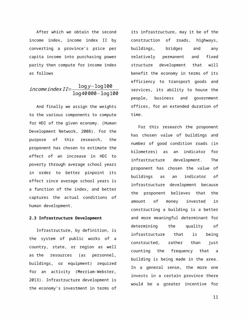
After which we obtain the second income index,

income index II by converting a province’s price per

capita income into purchasing power parity then

compute for income index as follows

incomeindex II= log y−log 100log 40 000−log 100

And finally we assign the weights to the various

components to compute for HDI of the given

economy. (Human Development Network, 2008). For

the purpose of this research, the proponent has

chosen to estimate the effect of an increase in HDI to

poverty through average school years in order to

better pinpoint its effect since average school years is

a function of the index, and better captures the actual

conditions of human development.

2.3 Infrastructure Development

Infrastructure, by definition, is the system of

public works of a country, state, or region as well

as the resources (as personnel, buildings, or

equipment) required for an activity (Merriam-

Webster, 2013). Infrastructure development is the

economy’s investment in terms of its infrastructure,

may it be of the construction of roads, highways,

buildings, bridges and any relatively permanent and

fixed structure development that will benefit the

economy in terms of its efficiency to transport goods

and services, its ability to house the people, business

and government offices, for an extended duration of

time.

For this research the proponent has chosen value

of buildings and number of good condition roads (in

kilometres) as an indicator for infrastructure

development. The proponent has chosen the value of

buildings as an indicator of infrastructure

development because the proponent believes that the

amount of money invested in constructing a building

is a better and more meaningful determinant for

determining the quality of infrastructure that is being

constructed, rather than just counting the frequency

that a building is being made in the area. In a general

sense, the more one invests in a certain province

there would be a greater incentive for getting a return

on investment. Since the infrastructure is created for

the benefit of the individuals interested in using it,

the value of the building would be a better indicator.

As for the proponent’s reason for choosing number of

good condition roads as another measure for

infrastructure development, the proponent

hypothesizes that having better roads means that

there is a more efficient transportation in the area,

and when there is a more efficient way of moving

from one place to another within the province, it

would be easier to make transactions and will be

beneficial to the community with regards to

providing general access to their communities. Hence

good quality roads are considered by the proponent

as an ideal measure for infrastructure development.

2.4 Human Capital

Human capital formation is truly an integral part

of measuring the development of a certain economy.

It is possible to have great infrastructure development

but without the optimal capital depth, one cannot

sustain its economic existence. Increase in the quality

of labour, investment in capital, increase in current

capital K t are but examples of capital deepening.

Given a steady state Economy with one kind of

capital good, capital deepening is defined as the case

7

wherein the per worker capital good stock is a

decreasing function of its own rate of interest . In

Neo-classical macroeconomics which focuses on

capital accumulation and its links to saving decisions,

the marginal condition f ' (k )=price and the rate of

return ( r+δ=f ' (k )) where r is the principal rate of

return and δ is the rate of depreciation, lead to a per

capital return that is higher than before (Hirota,

1979),

The basis of capital deepening is rooted in the

Harrod-Neutral production function, which is in its

basic form Y=F ( AL, K ), where Y is income, A

defined as the technological shifter, L defined as

labour and K is defined as capital (McEachern,

2012).

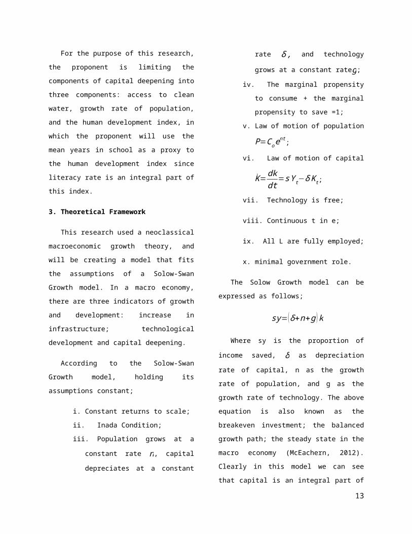
For the purpose of this research, the proponent is

limiting the components of capital deepening into

three components: access to clean water, growth rate

of population, and the human development index, in

which the proponent will use the mean years in

school as a proxy to the human development index

since literacy rate is an integral part of this index.

3. Theoretical Framework

This research used a neoclassical

macroeconomic growth theory, and will be creating a

model that fits the assumptions of a Solow-Swan

Growth model. In a macro economy, there are three

indicators of growth and development: increase in

infrastructure; technological development and capital

deepening.

According to the Solow-Swan Growth model,

holding its assumptions constant;

i. Constant returns to scale;

ii. Inada Condition;

iii. Population grows at a constant rate n,

capital depreciates at a constant rate δ , and technology grows at a constant rate

g;

iv. The marginal propensity to consume +

the marginal propensity to save =1;

v. Law of motion of population

P=Co ent;

vi. Law of motion of capital

K̇=dkdt

=sY t−δ K t;

vii. Technology is free;

viii. Continuous t in e;

ix. All L are fully employed;

x. minimal government role.

The Solow Growth model can be expressed as

follows;

sy=(δ +n+g ) k

Where sy is the proportion of income saved, δ as

depreciation rate of capital, n as the growth rate of

population, and g as the growth rate of technology.

The above equation is also known as the breakeven

investment; the balanced growth path; the steady

state in the macro economy (McEachern, 2012).

Clearly in this model we can see that capital is an

integral part of 3 variables: Depreciation of capital,

e.g. infrastructure, population, and technology.

Therefore capital can improve by affecting one of

these variables.

Now, since income is inversely related with

poverty, whereas an increase in income per capita in

8

an economy decreases the number of people living

below the poverty line, with of course assuming that

the increase in income is distributed among the

people of the economy. Since income is not our

immediate concern in this study and our dependent

variable that captures the effects of economic growth

is a poverty incidence, then the Solow growth model

is an essential primary tool to capture development.

As for our capturing variables within the Solow

growth, we use value of building constructions as

well as road development to capture infrastructure

development, and its contribution to the model is on

the depreciation rate of capital. As there is an

increase in infrastructure expenditure, then capital

infrastructure will depreciate less and less since

allocation of resources to infrastructure will decrease

wear-and-tear and will be more updated and efficient

(Estache, 2003) (Calderón & Servén, 2003).

As for human development, population growth

rate is affected by many factors, which include the

health and wellbeing of the people. As we have

reviewed in the literature, a human development

improvement will reduce poverty by increasing

income per capita, as individuals who are more

efficient tend to work better and provide better

opportunities for the person to grow, which in turn

improves the economy. We use years of schooling as

a capturing variable of human development, as

education is one of the most appalling reasons in the

literature that promote growth and development.

4. Empirical Analysis

4.1 Model Specification

For this research the regression model to be

formed is based on economic theories, research

materials gathered as well as the proponent’s

intuition. Using the classical linear regression model

through the ordinary least squares estimation, this

will establish the empirical portion of the theoretical

framework which will determine the empirical

validity of the research. This cross-section study

across the 78 provinces of the Philippines with the

initial semi log model specification, shown by the

following:

PI i=β1i+β2 ln Bldg i+β3 Roadi+β4 H 2Oi+β5 ni+ β6 Ed i+εi

4.2 A Priori Expectations

The following variables with their A Priori

expectations are presented in the following table:

PI Poverty incidence- the

percentage of the population

that is under the poverty line

per province of the

Philippines. Source: NSCB

ln B ldg Value of building

constructions for 2011- the

amount (in Php) used for the

development of buildings in

the provinces of the

Philippines. The proponent

opted to set in natural

logarithmic form to observe

percentage changes. Expected

to have a negative effect on

poverty incidence. Source:

NSO Quick Stats

Road Distance of good roads (in

km)- distance of road in

kilometres considered in good

condition by the Department

of Public Works and

Highways (DPWH).

9

Expected to have a negative

effect on poverty incidence.

Source: DPWH

H2O Percentage of households

with access to clean water.

Expected to have a negative

effect on Poverty Incidence.

Source: NSCB

n Population growth rate.

Expected to have a negative

effect on poverty incidence,

to be interpreted as additional

human capital. Source: NSO

Quick Stats

Ed Mean years of schooling (set

as a proxy for the 3

components of HDI).

Expected to have a negative

effect on poverty incidence.

Source: NSCB

4.3 Data Gathered

The data that the proponent will use is collected

from the National Statistical Coordination Board

(NSCB), the National Statistics Office (NSO), and

from the provinces Quick Stats, also taken from the

National Statistics Office, as well as the Department

of Public Works and Highways (DPWH) for the data

regarding the distance of DPWH at par with the

current standard of the department. Although the

dates are not exactly the same, this study is more

interested in averages through time, and since time is

not of the essence of this study, a simple cross section

is used.

5. Estimation and Inference

5.1 Summary of the Data

From the data gathered, 78 (with the exception

for the information gathered on DPWH which seems

to lack information on five provinces, namely

Basilan, Lanao del Sur, Sulu, Tawi-Tawi, and

Maguindanao) of the provinces have provided varied

statistics to the information needed in this research.

5.2 Regression of the Original Model

PI i=β1i+β2 ln Bldg i+β3 Roadi+β4 H 2Oi+β5 ni+ β6 Ed i+εi

Presented above is the original model

constructed. It consists of poverty incidence as the

dependent variable to the value of buildings

constructed, distance of DPWH certified good roads,

percentage of households with access to potable

water, population growth rate and the average years

in school which serves as a proxy to the HDI which is

a function of literacy index, life expectancy index and

the income index (see review of related literature).

The proponent used an Ordinary Least Square

(OLS) estimation method having all the Classical

Regression Model (CLM) assumptions met,

enumerated as follows:

a. Zero Mean Assumption i.e. E (ui )=μ=0;

b. Homoscedasticity i.e. var (u i )=σ 2 ;

c. No perfect Multicollinearity among all

independent variables;

d. Non- autocorrelation;

e. Zero covariance between independent

variables and the stochastic disturbance

term;

f. Number of observations should be greater

than number of parameters to be estimated;

g. Sufficient variation in the values of the

independent variables (Gujarati & Porter,

2009).

10

With the CLM assumptions taken into account

and met, then it according to Gauss and Markov, the

OLS estimate is the best linear unbiased estimator

(Carter Hill, Griffiths, & Lim, 2011). However for

this research, the proponent will only test for the

three critical assumptions, namely Multicollinearity,

Autocorrelation, and Homoscedasticity.

Running the regression analysis2, the estimated

coefficient values of the model are presented in the

generated model:

PI i=107.3815−0.0697046 lnBldgi−.0361233 Roadi−1.378105 H 2Oi−3.702187 ni−7.765788 Ed i+εi

5.3 Significant Statistical Findings on the Original

Model

The interpretation of the results generated has

provided some interesting and meaningful results. In

determining the validity of the model, one has to look

at the R-squared and the probability values of the

independent variables. First of all, we have to

consider the fact that all the a priori expectations for

every explanatory variable in the model have been

met- which proves that intuitively speaking the model

is correct.

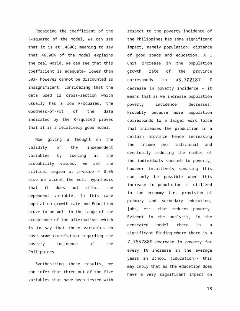
Regarding the coefficient of the R-squared of the

model, we can see that it is at .4606; meaning to say

that 46.06% of the model explains the real world. We

can see that this coefficient is adequate- lower than

50%- however cannot be discounted as insignificant.

Considering that the data used is cross-section which

usually has a low R-squared, the Goodness-of-Fit of

the data indicated by the R-squared proves that it is a

relatively good model.

Now giving a thought on the validity of the

independent variables by looking at the probability 2 Results in Appendix A

values, we set the critical region at p-value < 0.05

else we accept the null hypothesis that it does not

affect the dependent variable. In this case population

growth rate and Education prove to be well in the

range of the acceptance of the alternative- which is to

say that these variables do have some correlation

regarding the poverty incidence of the Philippines.

Synthesizing these results, we can infer that three

out of the five variables that have been tested with

respect to the poverty incidence of the Philippines

has some significant impact, namely population,

distance of good roads and education. A 1 unit

increase in the population growth rate of the province

corresponds to a3.702187 % decrease in poverty

incidence – it means that as we increase population

poverty incidence decreases. Probably because more

population corresponds to a larger work force that

increases the production in a certain province hence

increasing the income per individual and eventually

reducing the number of the individuals succumb to

poverty, however intuitively speaking this can only

be possible when this increase in population is

utilized in the economy i.e. provision of primary and

secondary education, jobs, etc. that reduces poverty.

Evident in the analysis, in the generated model there

is a significant finding where there is a7.765788%

decrease in poverty for every 1% increase in the

average years in school (Education)- this may imply

that as the education does have a very significant

impact on the poverty incidence of the Philippines.

For Roads, there is a .0361233% decrease in poverty

incidence for every 1 kilometre increase in the

distance of roads deemed by DPWH of good

condition, which may signify that there is a potential

decrease in poverty when roads are constructed.

5.4 Corrective Measures and Corrected Model

11

Since there is no problem in the model regarding

multicollinearity and heteroscedasticity, it is safe to

say that the model generated is indeed a good

approximate of what occurs in the real world3.

However it is in the best interest of the researcher to

find a better alternative model that has more

significant variables to better explain the

phenomenon of poverty.

Since the value of buildings and access to safe

water are clearly insignificant due to the results

generated, the best action to take is to find a way to

improve the model in such a way that more of these

intuitively sound components of poverty can result to

significant figures, statistically speaking. However

since there is no reason to do a corrected model, then

the proponent has no choice but to accept the model

as it is.

PI i=β1i+β2 ln Bldg i+β3 Roadi+β4 H 2Oi+β5 ni+ β6 Ed i+εi

With the following estimates:

PI i=107.3815−0.0697046 lnBldgi−.0361233 Roadi−1.378105 H 2Oi−3.702187 ni−7.765788Ed i+εi

6. Conclusion

I have presented a model that illustrates the

possible effects of infrastructure development and

capital deepening with respect to the poverty

incidence of the Philippines. In both the original and

corrected models, they have shown that there is

indeed a negative relationship between poverty and

the two determinants of growth and development,

thus verifying the macroeconomic theories behind the

model. In terms of the a priori expectations, it is safe

to say that the model fits these expectations, since in

3 See Appendix B.

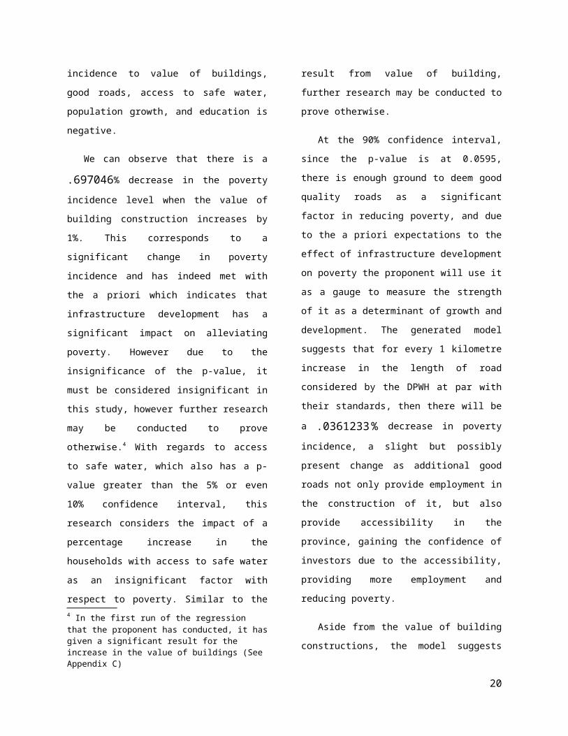
the empirical test the relationship of poverty

incidence to value of buildings, good roads, access to

safe water, population growth, and education is

negative.

We can observe that there is a .697046%

decrease in the poverty incidence level when the

value of building construction increases by 1%. This

corresponds to a significant change in poverty

incidence and has indeed met with the a priori which

indicates that infrastructure development has a

significant impact on alleviating poverty. However

due to the insignificance of the p-value, it must be

considered insignificant in this study, however

further research may be conducted to prove

otherwise.4 With regards to access to safe water,

which also has a p-value greater than the 5% or even

10% confidence interval, this research considers the

impact of a percentage increase in the households

with access to safe water as an insignificant factor

with respect to poverty. Similar to the result from

value of building, further research may be conducted

to prove otherwise.

At the 90% confidence interval, since the p-value

is at 0.0595, there is enough ground to deem good

quality roads as a significant factor in reducing

poverty, and due to the a priori expectations to the

effect of infrastructure development on poverty the

proponent will use it as a gauge to measure the

strength of it as a determinant of growth and

development. The generated model suggests that for

every 1 kilometre increase in the length of road

considered by the DPWH at par with their standards,

then there will be a .0361233 % decrease in

poverty incidence, a slight but possibly present

4 In the first run of the regression that the proponent has conducted, it has given a significant result for the increase in the value of buildings (See Appendix C)

12

change as additional good roads not only provide

employment in the construction of it, but also provide

accessibility in the province, gaining the confidence

of investors due to the accessibility, providing more

employment and reducing poverty.

Aside from the value of building constructions,

the model suggests that there is also a 3.702187%

decrease in poverty incidence for every 1 unit

increase in the growth rate of population.

Considering that this value is significant, there is a

corresponding decrease in poverty for an increase in

population can be interpreted in many ways- that

population should not be considered a problem given

that this human resource is utilized by provision of

education and employment, or that population is not a

problem at all and in fact we must promote an

increase in population, or that this research is merely

stating out the fact that the overpopulation issue does

not hold as much importance when it comes to

alleviating poverty- with this the research is limited

to.

The impact of education to poverty is indeed

econometrically significant. Having a probability

value to a point that it is negligible (at rounded off

0.000) it is indeed possible to infer that there could be

a 7.765788% decrease in poverty for every unit

increase in the average years of schooling. The

results generated by the econometric model clearly

demonstrates the macroeconomic theory in

education, that by Psacharopolous the more time

invested in education, the higher the rate of return,

thus aides in the alleviation of poverty (McEachern,

2012).

Regarding the coefficient of the R-squared of the

generated model, we can see that it is at .4606;

meaning to say that 46.06% of the model explains the

real world. We can see that this coefficient is

adequate- lower than 50%- however cannot be

discounted as insignificant. Considering that the data

used is cross-section which usually has a low R-

squared, the Goodness-of-Fit of the data indicated by

the R-squared proves that it is a relatively good

model.

The model’s results, which its findings can be

summarized as follows:

a. All a-priori expectations are met;

b. there may be a 3.70% decrease in

poverty incidence for every 1%

increase in the population (1 unit

increase in the growth of

population);

c. there could be a 7.77% decrease in

poverty incidence for every 1 unit

increase education;

d. there could be a .04 % reduction in

poverty incidence for every 1

kilometre increase in road

considered by DPWH at par with

their standards;

e. The model may explains 46.06% of

the real world;

f. No problems with the critical

assumptions of the classical linear

regression model.

The proponent has generated estimates of the

econometric model:

PI i=β1i+β2 ln Bldg i+β3 Roadi+β4 H 2Oi+β5 ni+ β6 Ed i+εi

13

Presented as follows:

PI i=107.3815−0.0697046 lnBldgi−.0361233 Roadi−1.378105 H 2Oi−3.702187 ni−7.765788 Ed i+εi

This study suggests that the best way to alleviate

poverty for the Philippine economy is for the

government to increase its allocation of budget on

educational programs, such as increasing the number

of public schools up to the secondary level, increase

the generation of scholarship programs in order to

further increase the number of graduates inclusive of

but not limited to academic scholarships, merit

scholarships and pay-it-forward programs that will

increase the literacy rate of the county. An increase in

population will actually lessen poverty if and only if

the additional increase in population will correspond

to an increase in education and job opportunities in

order to fully utilize the additional human resource.

Given these information, the proponent recommends

that the government should focus in projects

regarding the deepening of the pool of capital

available in the country that includes investment in

human capital in the form of education, as well as the

full utilization of the population.

It is also suggested that the government should

also increase its budget allocation on road

improvement to provide access to rural communities

in order to efficiently transport goods and services

from one point to another i.e. in an agricultural

business perspective, the goods produced will be

more efficiently transported from the farm, to the

local and urban marketplace and eventually to the

consumers. An increase in the value of building

constructions, though deemed insignificant in this

study, also proves to yield a negative impact on

poverty, which gives enough evidence, though

statistically insignificant for this research, to claim

that indeed a higher spending on building

constructions may lessen the population of the

impoverished by providing employment in the

construction of the buildings plus additional space for

businesses and local government units to provide

additional employment in the community. In order to

fully maximize these conditions, the government

must fully utilize its resources in order to maximize

the results of its projects to address the problem of

poverty in the country; that is to say that good

governance and clean auditing of government funds

must be integral in order for this model’s generated

result to be of any use, since in this study we assume

that good governance is a constant.

The model generated could not immediately be

judged as a failure due to the insignificance of

building construction and access to safe water,

although it is in the best interest of the proponent to

generate a greater amount of significant results rather

than the indicated beforehand. Throughout the

research, the proponent has not drifted away from the

sound economic theories that this study is based

upon, and the a priori expectations have always been

met.

Nevertheless, this study can serve as a

supplementary study, an addition to the studies made

with regard to the topic of poverty. Poverty is one of

the most pressing problems that humanity faces as a

race. In the world that we live in today, with all the

technological advancements and scientific

breakthroughs, it is integral to find ways in order to

reduce poverty in order to aide in the attainment of

United Nation’s Millennium Development Goals

where alleviation of poverty is one of them.

14

Appendix A.

Summary of the Data

From the data gathered, 78 (with the exception for the information gathered on DPWH which seems to lack information on five provinces,

namely Basilan, Lanao del Sur, Sulu, Tawi-Tawi, and Maguindanao) of the provinces have provided varied statistics to the information needed in this research. Presented hence is a summary of the information gathered:

Table 1. Data Summary

Variable Observations Mean S.D. Min MaxPoverty incidence 78 33.46154 14.55056 0 61.6

Value of building constructions 78 1604619 2650193 47121.50E+0

7Distance of good road 73 65.77438 57.60592 0 258.1Households w/ access to safe water 78 0.7822965 0.368596 0.009443 2.560873Population growth rate 78 1.620769 0.632611 0.08 4.12Average years in school (up to secondary) 78 8.455128 1.383732 4.6 12.6

Presented below is the summary of the results yielded using the data gathered from NSCB, NSO and DPWH. The results will be then examined for possible problems in heteroscedasticity, multicollinearity and autocorrelation. This table

displays the variables involved in the econometric model, with their corresponding estimated coefficients, probability values, standard deviations, and the coefficient of determination represented by the value of the R-squared.

Table 2. Dependent Variable: Poverty Incidence(OLS Estimation: Across 78 Provinces of the Philippines)

Significance5Value of Estimate

Constant *** 107.3815(s.e.) (11.02191)Value of building constructions (ln) -0.0697046(s.e.) (.8792123)Distance of good roads * -0.0361233(s.e.) (0.229012)Access to safe water -1.378105(s.e.) (3.605055)Population growth rate ** -3.702187(s.e.) (2.09804)Average years in school *** -7.765788(s.e.) (1.414965)Root MSE 11.028R-squared 0.4606

5 Legend: * -significant at the 10% level; ** -significant at the 5% level; *** -significant at the 1% level

15

Adjusted R-squared 0.4204F-Test *** 11.44 (5,67)Ramsey RESET 0.06556

Appendix B.

Testing for the Critical Assumptions

Multicollinearity

According to Gujarati & Porter (2009), multicollinearity is a fact of life; it cannot be removed or isolated. However it is possible for us to test whether or not the level of multicollinearity is tolerable, dangerous or perfect.

In the instance wherein there is perfect multicollinearity it is safe to assume that it would be impossible for any researcher to find any estimates for the X values, since their standard errors will be infinite (determinant will be zero). If

multicollinearity is less than perfect but at a dangerous level, this may result to bloated standard errors, insignificant p-values of the t statistics though the R-squared is deemed a fitting model; this results to a wholesale acceptance of the null hypothesis, which increases the probability of committing a type II error. This may cause the researcher to omit good regressors for the model since these X estimates will be deemed insignificant.

Presented below is the result of the multicollinearity test via analysis of the Variance-Inflating Factor, commonly known as the VIF:

Table 3. VIF Test

Variable VIF 1/VIFValue of building constructions (ln) 1.51 0.662259Average years in school (up to secondary) 1.45 0.687475Population growth rate 1.1 0.909241Households w/ access to safe water 1.08 0.924616Distance of good roads (DPWH) 1.03 0.97049

Mean VIF 1.24

To determine the severity of multicollinearity in the model, we must look at the generated values for the VIF whether or not they are greater than or equal to 10, otherwise the level of multicollinearity is tolerable. As we can see, all the VIF values generated are less than 10. Moreover the individual VIF’s tolerance levels, taken into account by 1/VIF are all greater than 10%. Therefore it is safe to conclude that the model has a tolerable level of multicollinearity.

Autocorrelation

The term autocorrelation may be defined as “correlation between members of series of observations ordered in time or space, simply put: E (ui u j )=0 This phenomenon causes an overestimation of the R-squared, as well as incorrect t-statistics as well as p-values. The root cause of this is from the underestimation of the standard errors, leading to wrong policy recommendations and counterintuitive signs in the econometric model. Since this research deals with a cross-section data, then there is no need to test for problems in

6 Ho: no omitted variable bias; H1: omitted variable bias present. Accept Ho at 95% level of significance.

16

autocorrelation since it only appears in time-series data. (Gujarati & Porter, 2009)

Homoscedasticity

Homoscedasticity is the equal spread of variances, symbolically speaking it is written as E (u i

2)=σ 2 , ∀ i=1,2 ,…,n. If plotted in a graph, the points should not follow a pattern. The problem of heteroscedasticity (or heteroskedasticity) is most

common in cross-section data. When Heteroscedasticity is not properly treated, it will cause the OLS to no longer be the Best Linear Unbiased Estimate (BLUE), since it causes the values of R-squared, t-stats, standard errors to be all wrong.

Using the Breusch-Pagan-Godfrey test for Heteroscedasticity, we obtain the following results:

Table 4. Breusch-Pagan test for heteroscedasticity

Ho: Constant varianceVariables: fitted values of poverty incidence

Chi-squared (1) 0.11Prob > Chi-squared 0.7379***

Decision: Accept Ho at 95% confidence interval

To interpret this result we must consider that given that the null hypothesis indicates homoscedasticity while the alternative indicates heteroscedasticity, if the Prob > chi2 presented in the test is greater than 0.05, the null hypothesis is accepted; which implies that the model exhibits homoscedasticity. Since the probability is at 0.7379-

significantly greater than the acceptance level at 0.05, then it is safe to accept the null hypothesis and say that there is homoscedasticity; which implies that there is no problem of heteroscedasticity in the model.

A similar result has come up with a generation of the White’s Test:

Table 5. White's Test for heteroscedasticity

Ho: homoscedasticityHa: unrestricted heteroscedasticitychi-squared (20) 14.1Prob > chi-squared 0.8256***

Decision: Accept Ho at 95% confidence interval

17

Appendix C.

Previous Test Run with corresponding VIF, Breusch-Pagan-Godfrey Test and White’s Test

Table 3. Dependent Variable: Poverty Incidence (natural log)(OLS Estimation: Across 78 Provinces of the Philippines)

Significance7Value of Estimate

Constant *** 4.97415

(s.e.) (.44817)

Value of building constructions (ln) ** -0.0816(s.e.) (.343216)Distance of good roads * -0.0011684(s.e.) (0.0010007)Access to safe water -0.1459578(s.e.) (0.1546506)Population growth rate *** -0.2838653(s.e.) (0.9415)HDI (ln) ** -0.2526639(s.e.) (0.0972426)

Root MSE .4765R-squared 0.3657Adjusted R-squared 0.3176

F-Test *** 7.61 (5,66)

VIF 1.108

***

7 Legend: * -significant at the 10% level; ** -significant at the 5% level; *** -significant at the 1% level8 Since VIF < 10, then tolerable level of multicollinearity

18

Breusch Pagan test Heteroscedasticity 0.0049

ReferencesCalderón, C., & Servén, L. (2003). The Effects of Infrastructure Development on Growth and Income Distribution. Washington,

D.C.: World Bank Policy Research Working Paper Number 3400.

Carter Hill, R., Griffiths, W. E., & Lim, G. (2011). Principles of Econometrics. New Jersey: John Wiley & Sons, Inc.

Estache, A. (2003). On Latin America’s Infrastructure Privatization and its Distributional Effects. Washington DC.: The World Bank, Mimeo.

GSRubio/PR and Information Services. (2013). CSC scores Top 1-2-3 grand slam in Nov. 2011 Civil Engineer Board Exam. Retrieved March 23, 2013, from Catanduanes State University Website: http://www.csc.edu.ph/news/112011/csc_scores_grandslam_ceboard.htm

Gujarati, D., & Porter, D. (2009). Basic Econometrics. New York: Mc-Graw Hill.

Hirota, M. (1979). Capital Deepening Response and Heterogeniety of Capital Goods. International Economic Review, 325.

Human Development Network. (2008). Computing for HDI. Retrieved March 23, 2013, from Human Development Network Website: http://hdn.org.ph/computing-for-hdi/

McEachern, W. A. (2012). Macroeconomics. Singapore: Cengage Learning Asia Pte. Ltd.

Merriam-Webster. (2013). Definition of infrastructure. Retrieved March 28, 2013, from Merriam-Wester Dictionary Website: http://www.merriam-webster.com/dictionary/infrastructure

National Statistical Coodrination Board. (2013). Human Development Index (HDI). Retrieved March 23, 2013, from National Statistical Coordination Board Website: http://www.nscb.gov.ph/technotes/hdi/hdi_tech_comp.asp

National Statistical Coordination Board. (2007). The best schools, the worst schools! NSCB.

National Statistical Coordination Board. (2013). Annual Per Capita Poverty Threshold, Poverty Incidence and. Retrieved March 27, 2013, from NSCB website: http://www.nscb.gov.ph/poverty/2009/table_1.asp

National Statistical Coordination Board. (2013, January 14). Catanduanes is top Bicol province in human development? Retrieved March 23, 2013, from National Statistical Coordination Board Website: http://www.nscb.gov.ph/ru5/products/factsheet/fs01s13.htm

Puraran Surf Beach Resort. (2013). About Puraran Beach. Retrieved March 23, 2013, from Puraran Surf Beach Resort website: http://www.puraransurf.com/about.html

UNDP. (2011). Human Development Report. UNDP.

World Bank. (2011). Choosing and Estimating Poverty Indicators. Retrieved March 28, 2013, from World Bank Website: http://web.worldbank.org/WBSITE/EXTERNAL/TOPICS/EXTPOVERTY/EXTPA/0,,contentMDK:20242881~menuPK:435055~pagePK:148956~piPK:216618~theSitePK:430367~isCURL:Y~isCURL:Y,00.html

9 Presence of heteroscedasticity

19

World Bank. (2011). Defining Welfare Measures. Retrieved March 28, 2013, from World Bank Website: http://web.worldbank.org/WBSITE/EXTERNAL/TOPICS/EXTPOVERTY/EXTPA/0,,contentMDK:20242876~menuPK:435055~pagePK:148956~piPK:216618~theSitePK:430367~isCURL:Y~isCURL:Y,00.html

World Bank. (2011). Defining Welfare Measures. Retrieved March 28, 2013, from World Bank Website: http://web.worldbank.org/WBSITE/EXTERNAL/TOPICS/EXTPOVERTY/EXTPA/0,,contentMDK:20242876~menuPK:435055~pagePK:148956~piPK:216618~theSitePK:430367~isCURL:Y~isCURL:Y,00.html

20