regional interpretation of water-quality monitoring data · regional interpretation of...

Regional interpretation of water-quality monitoring data

Richard A. Smith, Gregory E. Schwarz, and Richard B. AlexanderU.S. Geological Survey, Reston, Virginia

Abstract. We describe a method for using spatially referenced regressions ofcontaminant transport on watershed attributes (SPARROW) in regional water-qualityassessment. The method is designed to reduce the problems of data interpretation causedby sparse sampling, network bias, and basin heterogeneity. The regression equation relatesmeasured transport rates in streams to spatially referenced descriptors of pollution sourcesand land-surface and stream-channel characteristics. Regression models of totalphosphorus (TP) and total nitrogen (TN) transport are constructed for a region defined asthe nontidal conterminous United States. Observed TN and TP transport rates are derivedfrom water-quality records for 414 stations in the National Stream Quality AccountingNetwork. Nutrient sources identified in the equations include point sources, appliedfertilizer, livestock waste, nonagricultural land, and atmospheric deposition (TN only).Surface characteristics found to be significant predictors of land-water delivery include soilpermeability, stream density, and temperature (TN only). Estimated instream decaycoefficients for the two contaminants decrease monotonically with increasing stream size.TP transport is found to be significantly reduced by reservoir retention. Spatial referencingof basin attributes in relation to the stream channel network greatly increases theirstatistical significance and model accuracy. The method is used to estimate the proportionof watersheds in the conterminous United States (i.e., hydrologic cataloging units) withoutflow TP concentrations less than the criterion of 0.1 mg/L, and to classify catalogingunits according to local TN yield (kg/km2/yr).

1. Introduction

The objectives of regional water-quality assessments are todescribe spatial and temporal patterns in water quality andidentify the factors and processes that influence those condi-tions [National Research Council, 1994; Mueller et al., 1997].Some regional assessments have the specific purpose of relat-ing water quality to legal standards. Since its enactment in1972, the Federal Clean Water Act (Public Law 92-500) hasrequired state governments, river basin commissions, and thefederal government to estimate biennially the proportion ofsurface waters that meet accepted quality standards. Theseassessments, and numerous others called for in subsequentamendments to the act [Knopman and Smith, 1993], influencea myriad of regulatory decisions and the expenditure of billionsof dollars annually [U.S. Environmental Protection Agency,1990b].

Historically, a broad combination of state and federal mon-itoring networks and programs has served as the principalsource of data for assessments. Efforts to compile data frommultiple sampling stations for assessing water quality at thestate [Dole and Wesbrook, 1907; Van Winkle and Eaton, 1910],river basin [Leighton and Holister, 1904; Barrows and Whipple,1907], and national [Dole, 1909] levels can be traced to theearly 20th century. Since that time, network sampling programshave increased in number, size, and complexity [National Re-search Council, 1990] and now support regional water-qualityassessment activities at spatial scales ranging from local toglobal [e.g., Hirsch et al., 1988; Meybeck, 1982].

Despite widespread and long-standing interest in the use of

data from monitoring networks, certain commonly encoun-tered problems make it difficult to interpret point-level water-quality data in areal terms and thus meet the objectives ofregional water-quality assessments. Even when their objectivesare clearly established and sampling programs are wellplanned, regional water-quality assessments are often compli-cated by (1) sparseness of sampling locations due to cost con-straints, (2) spatial biases in the sampling network due to theneed to target sampling toward specific pollution sources, and(3) drainage basin heterogeneity. These complications impededata interpretation in distinct ways by limiting sample sizes,reducing the regional representativeness of the sampling net-work, and limiting the ability to relate in-stream conditions tospecific pollution sources.

In this paper, we describe a method for interpreting moni-toring data that reduces the commonly encountered problemsof network sparseness, bias, and basin heterogeneity. Themethod involves construction of a statistical model relatingwater-quality observations to spatially referenced (and poten-tially temporally referenced) data on basin attributes. The in-troduction of an explanatory model and ancillary data on basinattributes expands the information base for interpreting water-quality measurements, enhancing the ability both to describeregional conditions and identify causative factors.

Current methods for interpreting data from sampling net-works are based on relatively simple models of limited useful-ness in assessments because of the complications of networksampling. For example, estimates of the proportion of a waterresource meeting specified quality standards are generallybased on frequency-related interpretations of monitoring data;but such estimates are invalid when spatial or temporal sam-pling biases are large. Accurate estimates of proportions arecurrently achievable only through randomized sampling

This paper is not subject to U.S. copyright. Published in 1997 by theAmerican Geophysical Union.

Paper number 97WR02171.

WATER RESOURCES RESEARCH, VOL. 33, NO. 12, PAGES 2781–2798, DECEMBER 1997

2781

[Messer et al., 1991] or when an existing sampling network canbe shown through ex post analysis [Smith et al., 1993a] toprovide approximate estimates. In practice, however, strongincentives exist for conducting nonrandomized (i.e., targeted)sampling to determine the causes of poor water quality [Knop-man and Smith, 1993] or to take advantage of establishedmonitoring systems such as streamflow measuring networks.Thus, despite the important role that proportions play in le-gally mandated water-quality assessments, rigorous estimatesof proportions are rarely made.

Spatial-analytic techniques such as kriging [e.g., Clark, 1979;Hughes and Lettenmaier, 1981] are designed to interpret spatialgradients and account for spatial dependencies in data fromsampling networks. In theory, these techniques would providea basis for drawing maps of water-quality conditions and mak-ing unbiased estimates of proportions. However, these inter-polation techniques are not well suited to the dendritic natureof stream networks, and their usefulness for understanding thecauses of contaminated conditions is limited by the lack of trueexplanatory variables.

A variety of statistical methods has been used to relatenetwork-derived water-quality data to explanatory factors. Onesimple approach uses box plots to compare the distributions ofwater-quality measurements for groups of sampling stationsdifferentiated by land use or other basin attributes [Mueller etal., 1995; Smith et al., 1993a; see also Omernick, 1976]. Al-though causal links have been identified, basin heterogeneityusually limits the ability to clearly differentiate the effects ofspecific attributes, and the predictive power of the technique islow. Beginning with attempts to determine the factors influ-encing suspended sediment yields [Branson and Owen, 1970;Flaxman, 1972; Hindall, 1976], a variety of regression tech-niques have been used to relate water quality to basin at-tributes [Steele and Jennings, 1972; Lystrom et al., 1978; Steele,1983; Peters, 1984; Osborne and Wiley, 1988; Driver and Tasker,1990; Hainly and Kahn, 1996; Mueller et al., 1997]. However,these models treat basin attributes as homogeneously distrib-uted in the watershed, an assumption that fails to account forimportant relationships among the attributes and between theattributes and water-quality measurements on the dependentside of the regression equation. A recent paper by Cressie andMajure [1997] combines kriging techniques with a regressionmodel that recognizes a finite zone of influence within thewatershed, thus avoiding the strict homogeneous assumption.

The primary distinction between our method and previousregression approaches is our explicit inclusion of the spatialdimension in the underlying model. In the model developedhere, contaminant transport is described as a function of spa-tially referenced land-surface and stream-channel characteris-tics. An important, testable hypothesis of the present study isthat spatial referencing of basin attributes increases their cor-relation with water-quality measurements. A second, thoughless easily tested, hypothesis of this study is that spatial refer-encing facilitates the interpretation of model coefficients interms of the sources and processes involved in contaminanttransport through watersheds. As discussed and illustrated insection 4, this enhanced capability allows the model to beapplied to a variety of assessment-related problems not possi-ble with earlier approaches. We refer to the method describedhere as Spatially Referenced Regressions On Watershed at-tributes (SPARROW).

The SPARROW method described here includes severalmodifications and refinements of a prototype method for spa-

tially referenced regressions of water-quality measurements onbasin attributes previously described by Smith et al. [1993b].The principal differences between the earlier study and thisone are the consideration of more varied sources of pollution,additional processes affecting the delivery of these sources, abetter statistical treatment of the decay process, and the ap-plication of the model to a larger region with a more diverserange of basin sizes and characteristics. The present model isbased on data from approximately 400 monitoring stations inthe National Stream Quality Accounting Network [Alexander etal., 1996; Ficke and Hawkinson, 1975] and is applied to nontidalstream reaches in the conterminous United States.

To demonstrate use of the model in the context of regionalwater-quality assessment, we undertake two applications. Bothfocus on important estimation problems that are difficult toresolve with network-derived monitoring data alone. The firstis that of estimating the proportion of streams in regions of theconterminous United States in which the concentration of acontaminant exceeds an established criterion or threshold con-centration. As discussed above, accurate estimates of such pro-portions are an important goal of federally mandated assess-ments under the Clean Water Act but are difficult to obtainwhen spatial biases exist in the sampling network. We showthat the model developed here can be used to overcome theeffects of spatial sampling biases in estimating the proportionof U.S. watersheds (i.e., hydrologic cataloging units [Seaber etal., 1987]) having phosphorus concentrations at the watershedoutflow that exceed the commonly accepted criterion of 0.1mg/L.

The second application illustrates a method for prioritizingwatersheds for nonpoint-source pollution controls. Currently,there is considerable interest in increasing the efficiency ofpollution control programs, especially nonpoint-source controlprograms, by focusing control efforts on watersheds where theyare most needed. Stream monitoring alone does not providesufficient information to compare watersheds because the ef-fects of local pollution sources on in-stream water quality can-not be separated from the effects of contaminants originatingin upstream watersheds. We show that the spatially referencedmodel developed here can be used to compare the hydrologiccataloging units on the basis of local nutrient yields. Throughthe use of “bootstrap” methods [Efron, 1982], we obtain robustestimates of the accuracy of these predictions.

The paper is organized into five sections. Following theintroduction, a methods section includes a mathematical de-velopment of the underlying model and a description of thedata sets and statistical procedures used to build the model.Section 3 presents the results of the regression and error anal-yses and includes a description of the bootstrap proceduresused in error analysis. Section 4 presents the two model appli-cations, and section 5 contains a summary discussion.

2. Methods2.1. Overview of the Method

This section describes construction of a statistical modelrelating in-stream water-quality measurements to spatially ref-erenced watershed attributes. Spatial referencing of land-based and water-based variables is accomplished via superpo-sition of a set of contiguous land-surface polygons on adigitized network of stream reaches that define surface-waterflow paths for the region of interest. Water-quality measure-ments are available from monitoring stations located in a sub-

SMITH ET AL.: REGIONAL INTERPRETATION OF WATER-QUALITY DATA2782

set of the stream reaches. Water-quality predictors in themodel are developed as functions of both reach and land-surface attributes and include quantities describing contami-nant sources (point and nonpoint) as well as factors associatedwith rates of material transport through the watershed (such assoil permeability and stream velocity). Predictor formulae de-scribe the transport of contaminant mass from specific sourcesto the downstream end of a specific reach. Loss of contaminantmass occurs during both overland and in-stream transport. Incalibrating the model, measured rates of contaminant trans-port are regressed on predicted transport rates at the locationsof the monitoring stations, giving rise to a set of estimatedlinear and nonlinear coefficients from the predictor formulae.Once calibrated, the model is used to estimate contaminanttransport and concentration in all stream reaches. A variety ofregional characterizations of water-quality conditions are thenpossible based on statistical summarization of reach-level es-timates.

2.2. Model Development

The mathematical core of the SPARROW method is a re-lation that expresses the in-stream load (i.e., transport rate) ofa contaminant at the downstream end of a given reach as thesum of monitored and unmonitored contributions to the loadat that location from all upstream sources.

Let J(i) represent the set of reaches j that includes reach iand all upstream reaches except those that either contain orare located upstream of monitoring stations upstream of i(Figure 1). We define

Li 5 On51

N

Sn,i (1)

where Li is contaminant transport in reach i , Sn ,i is the con-taminant load from source n delivered to reach i from allreaches in the subbasin delineated by J(i).

In general, the N sources referred to in (1) include all types

of point and nonpoint sources of the contaminant in the regionof interest. We assume that monitoring stations are locatednear the downstream end of the reaches that contain them.Thus in-stream contaminant loads at the location of monitor-ing points upstream of i enter J(i) and are included as one ofthe N sources. We refer to these entering in-stream loads as“monitored sources” (see Figure 1).

The source terms Sn ,i includes the effects of a two-stagedelivery process operating on the contaminant mass as itmoves through the watershed. The first stage dictates the pro-portion of contaminant mass that is delivered from the landsurface to the channel network at reach j . For nonpointsources the first-stage delivery process is mediated by a vectorof reach-specific land-surface characteristics Zj, which influ-ence land-water delivery. Point sources and monitored sourcesenter reach j directly and are not influenced by Zj. The secondstage of the delivery process, applicable to point sources, non-point sources, and “monitored sources” (see above), deter-mines the proportion of contaminant present in the channel inreach j that is transported to reach i . This in-stream deliveryprocess is assumed to result from first-order decay of contam-inant mass expressed as a function of a vector of channelcharacteristics Ti , j. These channel characteristics, evaluatedover the entire channel length from reach j to reach i , includetime-of-travel and channel size. Thus the source terms Sn ,i areexpressed as

Sn,i 5 Oj[J~i!

sn, jDn~Zj! K~Ti, j! (2)

where sn , j is a measure of the contaminant mass from sourcen that is present in the drainage to reach j , Dn(Zj) is theproportion of sn , j that is delivered to reach j as a function ofland-surface characteristics Zj, and K(Ti , j) is the proportionof contaminant mass present in reach j that is transported toreach i as a function of channel characteristics Ti , j.

In distributing the land-surface contaminant source data tostream reaches, the quantities sn , j are obtained as the reported

Figure 1. Schematic diagram of stream reaches in relation to monitoring stations (reaches extend from onetributary junction to another). In calibrating the model, reach i refers to any reach containing a monitoringstation. In applying the model, reach i refers to any reach where a prediction is made. J(i) represents the setof reaches that includes reach i and all upstream reaches except those that either contain or are locatedupstream of monitoring stations upstream of i .

2783SMITH ET AL.: REGIONAL INTERPRETATION OF WATER-QUALITY DATA

quantity of contaminant from source n present in the land-surface polygon containing reach j times the ratio of the lengthof reach j to the total length of all reaches in the polygon. Thatis, if P( j) is the set of all reaches in the polygon containingreach j ,

sn, j 5 snS l jY Oj[P~ j!

l jD (3)

where sn is the reported quantity of contaminant from sourcen present in the land-surface polygon containing reach j and l j

is the length of reach j .Empirical implementation of the model given in (1) and (2)

requires an explicit functional form for the delivery factorsDn(Zj) and K(Ti , j). The land-water delivery factor is param-eterized as

Dn~Zj! 5 bn exp ~2a9Zj!

Dn~Zj! 5 bn (4)

Dn~Zj! 5 1

for nonpoint sources, point sources, and upstream monitoredloads, respectively, where bn is a source-specific coefficientand a is a vector of delivery coefficients associated with theland-surface characteristics Zj.

Because reported contaminant-source data may include sur-rogate measures or may understate or overstate the true avail-ability of contaminant mass, the coefficients bn may deviatefrom unity. Also, the land-surface characteristics Zj may beeither positively or negatively related to contaminant delivery.If a land-surface characteristic is thought to be positively re-lated to delivery (stream density, for example), its element ofZj is taken to be the reciprocal of the characteristic, and if aland-surface characteristic is thought to be negatively relatedto delivery (soil permeability, for example), its element of Zj istaken to be the characteristic itself. In either case, the land-water delivery coefficients a are expected to be positive.

The polygon-based land-surface characteristics Zj are dis-tributed to stream reaches by assuming the land-surface char-acteristic for reach j to be equal to the sum of the length-weighted land-surface characteristic of all polygons associatedwith reach j . Thus, if P( x) is the set of all polygons containingreach j ,

Zj 5 Oj[P~ x!

~ zx, j l x, j /l j! (5)

where zx , j is the land-surface characteristic of polygon x asso-ciated with reach j , lx , j is the length of the portion of reach jassociated with polygon x , and l j is the total length of reach j .

The in-stream delivery terms K(Ti , j) are parameterized as

K~Ti, j! 5 exp ~2d9Ti, j! (6)

where d is a vector of first-order decay coefficients associatedwith the flow path characteristics Ti , j. Details of the specificform of the Ti , j are discussed in section 2.5.

2.3. Estimation of the Model

An estimable version of the model given by (1), (2), (4), and(6) is obtained by introducing a multiplicative error term e«,where « i is assumed to be independent and identically distrib-uted across nonoverlapping subbasins. Applying a logarithmictransformation of (1), we obtain the estimable model

Li 5 ln S On51

N

Sn,iD 1 « i (19)

where Li is the natural logarithm of transport. The deliveredsources Sn ,i appearing in (19) continue to be given by (2), (4),and (6). Coefficient estimation was performed using the modelprocedure by SAS Institute [1993].

The assumption that the error term « i is independent acrossobservations implies there is no correlation in the errorsamong the monitored basins. This assumption is consistentwith the way the model treats nested basins. When one mon-itored basin contains another monitored basin, the model usesthe monitored transport from the upstream basin (rather thanthe model-estimated transport) to represent contaminantsources entering the lower basin. Thus prediction errors thatoccur at the upstream monitored site do not cascade down tothe lower monitored site and do not induce correlation acrossthe subbasin error terms.

The following sections describe the contaminant sources,land-surface characteristics, and channel characteristics in themodel, and their anticipated statistical relationship to contam-inant transport. The data sources used in model calibration arealso described.

2.4. River Reach Network

A 1:500,000-scale digital stream network for the contermi-nous United States (River Reach File 1-RF1 [DeWald et al.,1985] defines surface water flow paths during model calibra-tion and prediction. The network consists of approximately60,000 reaches representing approximately 1 million km oftotal channel length (mean reach length is 17 km). Reachattributes include estimates of mean streamflow and watervelocity [DeWald et al., 1985]. Average stream velocity wasestimated for each reach using regression equations relatingvelocity to long-term mean streamflow and stream order. Theregressions were calibrated using U.S. Geological Survey time-of-travel studies. The reaches associated with 2100 large res-ervoirs (normal capacity greater than 5000 ac ft (1 ac ft 5 1233m3) [see Ruddy and Hitt, 1990]) were also designated in thereach attribute file. Finally, the stream network contains nu-merous instances of diversions and stream braiding. Thesefeatures were incorporated into the model with the assumptionthat contaminant concentration is uniformly distributed in thechannel cross section. Thus, if a diversion diverts 20% ofstreamflow, it is also assumed to divert 20% of the load pre-dicted at the point of the diversion.

2.5. Channel Transport Characteristics

In-stream losses of contaminant mass occur as a function ofthree variables: the travel time, streamflow (serving as a sur-rogate for channel depth), and whether or not the reach is partof a reservoir. Travel time is computed as the ratio of reachlength over stream velocity. Because the major processes in-volved in in-stream loss of total phosphorus (TP) and totalnitrogen (TN) (sedimentation and denitrification) operate atthe channel bottom, deeper streams are expected to have lowerrates of decay [Howarth et al., 1997]. To incorporate this effect,we divide streams into three flow classes: ,28.3 m3/s (1000ft3/s), 28.3–283 m3/s and .283 m3/s (10,000 ft3/s). We thenseparate the time of travel between reach i and reach j into thetotal time of travel over each of the three classes of streams.Thus the flow path characteristics vector Tij consists of three


variables representing the travel times associated with trans-port in the three stream classes. A network climbing algorithm[White et al., 1992] performs the required accumulation. Inestimating the decay coefficients (d in (6)), we expect mono-tonically decreasing values with increasing streamflow (i.e.,increasing channel depth).

TP retention in reservoirs may be expected to differ from TPdecay in streams because of differences in settling rates ofsediment-bound phosphorus in the two environments. To es-timate this effect, we define a fourth stream class in the TPmodel consisting of reaches that are classified as reservoirs.Accordingly, a fourth element is included in the flow pathcharacteristics vector Tij, consisting of the time of travel inreservoir reaches between reach i and reach j . Reservoirreaches are excluded when computing time of travel for thethree flow class variables. Exploratory regressions showed res-ervoir retention is not a significant factor in channel decay ofTN.

2.6. Dependent Variable Data

Data from the U.S. Geological Survey’s (USGS) NationalStream Quality Accounting Network (NASQAN) were used todevelop observational data for model calibration. Commenc-ing during the period 1973–1978, NASQAN records consist ofquarterly to monthly water column measurements from ap-proximately 400 stations located near the outlets of selectedU.S. hydrologic cataloging units [Alexander et al., 1996; Seaberet al., 1987]. Stations with indeterminant drainage area andstations with significant Mexican or Canadian drainage werenot used in the analysis. We estimated long-term mean annualtransport for TP and TN (sum of dissolved nitrate 1 nitrite andtotal Kjeldahl nitrogen measurements) at NASQAN stationsusing bias-corrected, log-linear regression-based load-estimation techniques [Cohn et al., 1989, 1992; Gilroy et al.,1990]. We modeled the total nutrients TN and TP rather thantheir component species because source data are generallyunavailable for the latter.

Periodic instantaneous measurements of nutrient transportfor the period 1974–1989 (or period of record for stations withshorter records; the number of observations ranged from 60 to120) were regressed on a set of up to five explanatory variables.The full model is of the form

ln ~L! 5 l0 1 l1t 1 l2 sin ~2pt! 1 l3 cos ~2pt! 1 l4 ln ~q!

1 l5 @ln ~q!#2 1 e (7)

where L is the instantaneous nutrient transport, t is decimaltime, q is instantaneous discharge, e is the sampling and modelerror assumed to be independent and identically distributed, lnis the natural logarithm, sin (2pt) and cos (2pt) are trigono-metric functions that jointly approximate seasonal variations intransport, and the l are regression coefficients. The modelwith the minimum prediction error sum of squares (PRESS[Montgomery and Peck, 1982]) was selected as the “best” fitfrom among the 15 possible models (seasonal terms enter andexit as a pair).

Using the regression parameters from (7), we estimated theannual transport that would have occurred at each station in1987 if streamflow had corresponded to average conditionsover the period 1970–1988. These estimates of mean annualtransport for the base year 1987 (L) become the dependentvariable in the SPARROW calibrations described below, andare obtained as

L 51

365 Od51

365

exp @l0 1 l1t9d 1 l2 sin ~2pt9d! 1 l3 cos ~2pt9d!

1 l4 ln qd 1 l5~ln qd!2# gm,d (8)

where qd is the mean of daily streamflow values for the dth dayof the year over the 1970–1988 period, t9d is decimal time forthe dth day in 1987, and gm ,d is the minimum variance bias-correction factor of Bradu and Mundlak [1970; see Cohn et al.,1989; Gilroy et al., 1990], where m is the degrees of freedom ofthe best fit regression based on (7).

To reduce the effects of measurement error in theSPARROW calibrations, we excluded stations where the stan-dard error of transport estimation was larger than 20% of themean estimated transport. TN calibrations were based on atotal of 414 stations, and TP calibrations were based on 381stations.

2.7. Contaminant Source Data

Five specific contaminant sources are included in the TNand TP models calibrated in this study: point sources, appliedfertilizers, livestock wastes, runoff from nonagricultural land,and atmospherically deposited nitrogen. (The atmosphere isassumed to be a negligible source of total phosphorus.) Asdescribed above, measurements of TN and TP transport atupstream monitoring sites are included in the model as in-stream sources of contaminant for downstream sites. This sec-tion describes the sources in greater detail and explains howthey appear in the model.

Contaminant-source data were obtained for years corre-sponding as close as possible to 1987, the year specified in (8)as the base year for transport estimation at monitoring sta-tions. Data for land-distributed sources were obtained as po-lygonal files representing either counties, cataloging units,physiographic regions, or contoured surfaces derived throughspatial interpolation of point data.

County-based estimates of the nitrogen and phosphoruscontent of applied fertilizers [W. Battaglin and D. Goolsby,U.S. Geological Survey, written communication, 1996; U.S.Environmental Protection Agency, 1990a] and livestock wasteswere obtained for 1987. The nitrogen and phosphorus contentof livestock wastes was estimated using 1987 Census of Agri-culture farm-animal population counts [U.S. Bureau of Census,1989] and estimates of per-animal nutrient production rates[U.S. Soil Conservation Service, 1992].

Estimates of atmospheric wet deposition of nitrate weredetermined through a linear spatial interpolation of 1987 meandeposition at 188 wet-fall monitoring stations in the NationalAtmospheric Deposition Program [National Atmospheric Dep-osition Program, 1988, written communication, 1995]. Becausewet nitrate deposition represents only a fraction of total nitro-gen deposition (recent data suggest that total deposition maybe 3–4 times wet nitrate deposition [Stensland et al., 1986]), thesource coefficient for atmospheric deposition is expected toexceed unity.

In addition to those identified above, we include an addi-tional nonpoint source representing contaminants contained inthe runoff from all types of nonagricultural land. The magni-tude of this source is assumed to be proportional to the totalarea of urban, forest, and range land in the basin as given bythe National Resources Inventory county estimates of landcover for 1987 [U.S. Soil Conservation Service, 1989]. Because


the data used to represent this source are not expressed inmass units, the source coefficient is not expected to approxi-mate unity.

County-based estimates of point-source discharges of totalphosphorus and Kjeldahl nitrogen [Gianessi and Peskin, 1984]were obtained from an inventory of 32,000 point-source facil-ities, including industries, municipal wastewater treatmentplants, and small sanitary waste discharges for the years 1977–1981. This inventory represents the most recent nationallycomprehensive compilation of point-source discharges of ni-trogen and phosphorus. Reach-level point-source dischargeestimates were obtained by disaggregating county-level esti-mates to reaches in proportion to the population density in thevicinity of the reaches. Reach-level estimates of 1980 popula-tion density [U.S. Bureau of Census, 1983] were determined byassigning the census-unit population to the nearest reachwithin 10 km and located in the same cataloging unit. Contam-inant loads from point sources are delivered directly tostreams, and the land-water delivery factor, e(2aZj), is notapplied. If the point-source data used in the regressions wereperfectly accurate, we would expect the source-specific coeffi-cient bn to equal unity. However, available national-level dataon point-source discharges of total nitrogen and total phos-phorus [Gianessi and Peskin, 1984] refer to 1977–1981 condi-tions and, in many cases, are estimated from information ontype of facility. Thus we do not restrict the source-specificcoefficient for point sources.

Because the “monitored sources” (see above) emanatingfrom upstream basins are, effectively, in-stream sources, theirland-water delivery factor is constrained to unity. However,these loads are “decayed” according to the same in-streamprocesses assumed for all other sources. The fact that moni-tored transport rates appear on the predictive (as well as theresponse) variable side of the regression equation makes itimportant that transport be measured accurately. The accuracyfilter applied to the transport estimates (see above) assuresthat this is so.

2.8. Land Surface Characteristics

Eight land surface characteristics are included as potentialland-water delivery factors (Zj in (4)) in SPARROW calibra-tions: soil permeability, slope, stream density, fraction of totalarea classified as wetlands, long-term average ambient air tem-perature, long-term mean precipitation, fraction of croplandthat is irrigated, and inches of applied irrigation.

Areas with highly permeable soils are expected to “absorb”contaminants readily and divert them to the subsurface. Thushigh rates of soil permeability are expected to decrease thedelivery of contaminants to streams. Cataloging unit-basedestimates of permeability were determined from digital data inthe State Soil Geographic (STATSGO) database [U.S. SoilConservation Service, 1994; Schwarz and Alexander, 1995]. Av-erage depth-weighted permeability was computed for approx-imately 78,000 STATSGO soil geographic units and was sum-marized by cataloging unit.

Land surface slope is included in calibrations in the recip-rocal form, implying an expected positive effect on contami-nant delivery. This assumption is consistent with the view thathigher velocities associated with steeper slopes decrease theeffects of time-dependent decay processes. We note, however,that steeper slopes may also produce more subsurface flow[Dunne and Leopold, 1978], thereby reducing the delivery ofcontaminants. The source and methods of compilation of land-

surface slope data are the same as for soil permeability[Schwarz and Alexander, 1995].

Stream density, defined as the ratio of channel length todrainage area, is included in the reciprocal form, indicating apositive effect on land-water delivery. A greater stream densityimplies land-surface contaminants travel shorter distances onaverage to reach streams. Estimates of stream density are com-puted directly from the length and area attributes of the streamnetwork coverage.

Wetlands are widely recognized as effective filters for re-moving nutrients and are especially effective in removing ni-trogen [Howarth et al., 1996; Seitzinger, 1988]. To account forthis potential effect, we include the fraction of the land surfaceclassified as wetlands as an element of the delivery vector Zj.County-level estimates of wetland area are taken from the1987 National Resources Inventory [U.S. Soil Conservation Ser-vice, 1989].

Higher temperatures increase rates of denitrification [Seitz-inger, 1988] and are expected therefore to decrease the deliveryof TN to streams. Higher temperatures would also be expectedto increase rates of nitrogen fixation, but because natural fix-ation is a relatively minor source of new nitrogen in mostwatersheds compared to cultural sources, and because denitri-fication is by far the most important sink for TN, we expect anoverall negative effect of temperature on TN delivery. Becausethe most important processes affecting the transport of TP arephysical rather than biochemical, we expect temperature tohave an insignificant effect on TP delivery. Nevertheless, tem-perature is included as a potential delivery factor in the ex-ploratory regressions for both TN and TP. Average ambient airtemperature was obtained for 350 climate divisions in the con-terminous United States for the period 1951–1980 [U.S. Geo-logical Survey, 1986].

High rates of precipitation were expected to speed the de-livery of contaminants to the stream network, resulting inhigher transport rates. In this case, precipitation would bepositively associated with delivery and should be included inthe delivery vector Zj in reciprocal form. However, preliminaryanalyses showed complications in using simple precipitation asan explanatory variable. Arid areas of the country with highrates of irrigation and low levels of precipitation, in somecases, have relatively high contaminant loads due, perhaps, tothe efficiency with which irrigation runoff is returned to thestream. In any case, precipitation appeared to be inverselyrelated to transport, and irrigation rate was poorly correlatedwith transport.

In an attempt to better isolate the separate effects of irriga-tion and precipitation, we formed two interaction variables.The first variable consisted of the reciprocal of applied irriga-tion (in inches per year) times the share of cropland that isirrigated. The second variable was the reciprocal of precipita-tion times the share of cropland that is not irrigated. Simulta-neous inclusion of both variables might be expected to capturethe separate effects of irrigation and precipitation on delivery.However, in many areas, irrigation is used as a supplement forprecipitation. In such areas, the amount of runoff from fields isrelatively constant, regardless of the level of irrigation. Toallow for this effect, we included as a third variable the shareof cropland that is irrigated.

The source for mean annual precipitation data is the same asthat for temperature data [U.S. Geological Survey, 1986].County estimates of annual irrigation water use were obtainedfor 1985 from U.S. Geological Survey data files [Smith et al.,


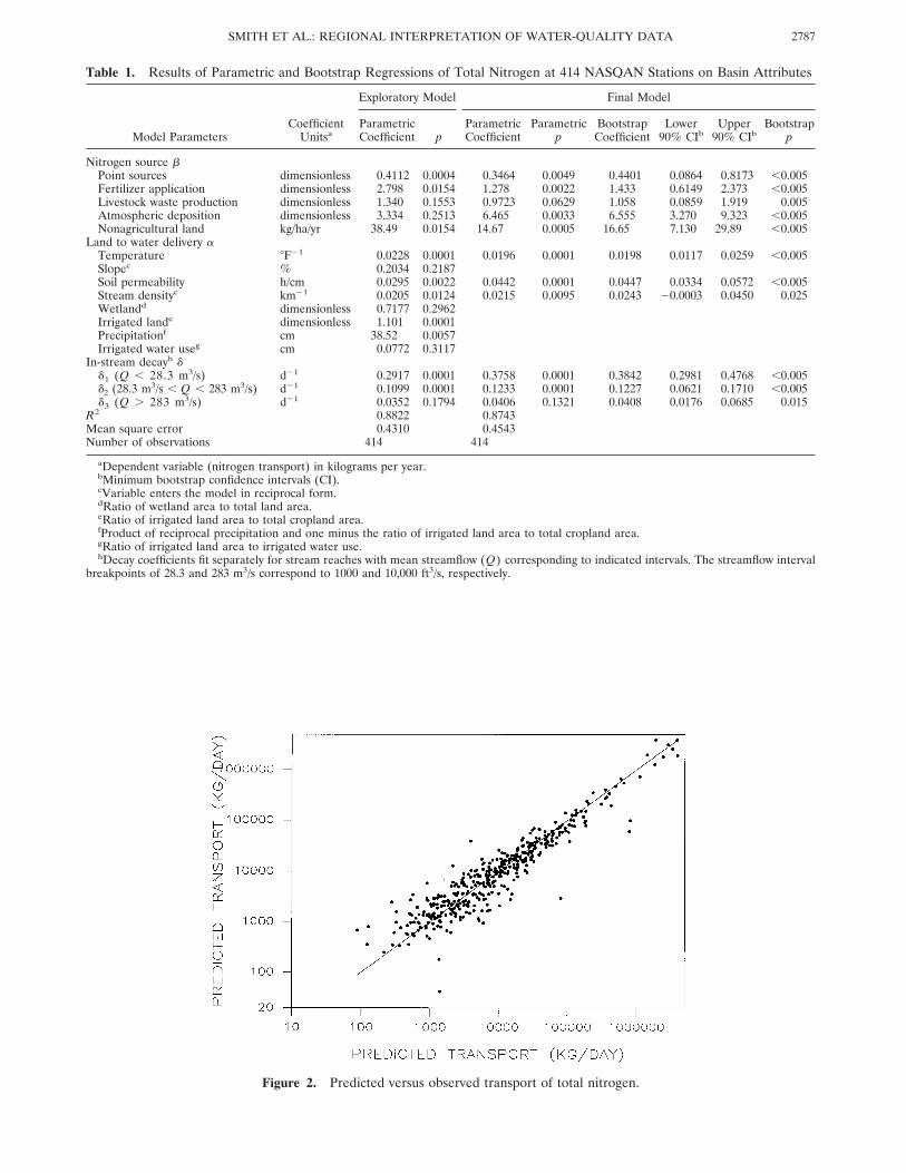
Figure 2. Predicted versus observed transport of total nitrogen.

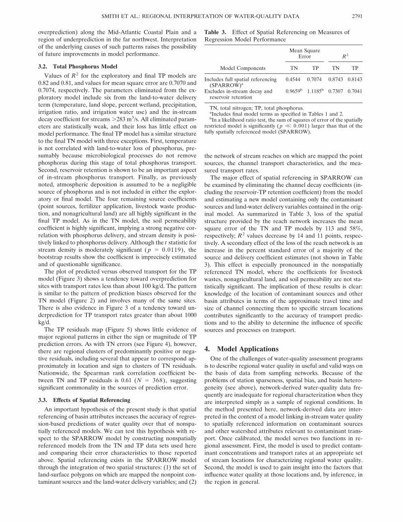
Table 1. Results of Parametric and Bootstrap Regressions of Total Nitrogen at 414 NASQAN Stations on Basin Attributes

Model ParametersCoefficient

Unitsa

Exploratory Model Final Model

ParametricCoefficient p

ParametricCoefficient

Parametricp

BootstrapCoefficient

Lower90% CIb

Upper90% CIb

Bootstrapp

Nitrogen source bPoint sources dimensionless 0.4112 0.0004 0.3464 0.0049 0.4401 0.0864 0.8173 ,0.005Fertilizer application dimensionless 2.798 0.0154 1.278 0.0022 1.433 0.6149 2.373 ,0.005Livestock waste production dimensionless 1.340 0.1553 0.9723 0.0629 1.058 0.0859 1.919 0.005Atmospheric deposition dimensionless 3.334 0.2513 6.465 0.0033 6.555 3.270 9.323 ,0.005Nonagricultural land kg/ha/yr 38.49 0.0154 14.67 0.0005 16.65 7.130 29.89 ,0.005

Land to water delivery aTemperature 8F21 0.0228 0.0001 0.0196 0.0001 0.0198 0.0117 0.0259 ,0.005Slopec % 0.2034 0.2187Soil permeability h/cm 0.0295 0.0022 0.0442 0.0001 0.0447 0.0334 0.0572 ,0.005Stream densityc km21 0.0205 0.0124 0.0215 0.0095 0.0243 20.0003 0.0450 0.025Wetlandd dimensionless 0.7177 0.2962Irrigated lande dimensionless 1.101 0.0001Precipitationf cm 38.52 0.0057Irrigated water useg cm 0.0772 0.3117

In-stream decayh dd1 (Q , 28.3 m3/s) d21 0.2917 0.0001 0.3758 0.0001 0.3842 0.2981 0.4768 ,0.005d2 (28.3 m3/s , Q , 283 m3/s) d21 0.1099 0.0001 0.1233 0.0001 0.1227 0.0621 0.1710 ,0.005d3 (Q . 283 m3/s) d21 0.0352 0.1794 0.0406 0.1321 0.0408 0.0176 0.0685 0.015

R2 0.8822 0.8743Mean square error 0.4310 0.4543Number of observations 414 414

aDependent variable (nitrogen transport) in kilograms per year.bMinimum bootstrap confidence intervals (CI).cVariable enters the model in reciprocal form.dRatio of wetland area to total land area.eRatio of irrigated land area to total cropland area.fProduct of reciprocal precipitation and one minus the ratio of irrigated land area to total cropland area.gRatio of irrigated land area to irrigated water use.hDecay coefficients fit separately for stream reaches with mean streamflow (Q) corresponding to indicated intervals. The streamflow interval

breakpoints of 28.3 and 283 m3/s correspond to 1000 and 10,000 ft3/s, respectively.


Figure 3. Predicted versus observed transport of total phosphorus.

Table 2. Results of Parametric and Bootstrap Regressions of Total Phosphorus Transport at 381 NASQAN Stations onBasin Attributes

Model ParametersCoefficient

Unitsa

Exploratory Model Final Model

ParametricCoefficient p

ParametricCoefficient

Parametricp

BootstrapCoefficient

Lower90% CIb

Upper90% CIb

Bootstrapp

Phosphorus source bPoint sources dimensionless 0.2507 0.0010 0.2972 0.0003 0.3033 0.0914 0.4651 ,0.005Fertilizer application dimensionless 0.1242 0.0847 0.1267 0.0035 0.1332 0.0398 0.2042 ,0.005Livestock waste production dimensionless 0.1640 0.0976 0.1973 0.0003 0.1884 0.1019 0.2821 ,0.005Nonagricultural land kg/hectare/yr 0.3505 0.0461 0.4092 0.0001 0.4236 0.2769 0.5937 ,0.005

Land to water delivery aTemperature degrees 8F.21 20.0058 0.4471Slopec percent 20.0243 0.8338Soil permeability hour/cm 0.0348 0.0068 0.0441 0.0001 0.0501 0.0262 0.0736 ,0.005Stream densityc km21 0.0467 0.0050 0.0401 0.0119 0.0290 20.0196 0.0630 0.185Wetlandd dimensionless 0.9229 0.3222Irrigated lande dimensionless 0.0704 0.8034Precipitationf cm 17.63 0.3481Irrigated water useg cm 0.0716 0.4347

In-stream decayf dd1 (Q , 28.3 m3/s) day21 0.2391 0.0001 0.2584 0.0001 0.2680 0.1885 0.3497 ,0.005d2 (28.3 m3/s , Q , 283 m3/s) day21 0.0905 0.0342 0.0947 0.0271 0.0956 0.0156 0.1834 0.010d3 (Q . 283 m3/s) day21 20.0276 0.5819d4 (reservoir retention)i day21 0.3378 0.0001 0.3377 0.0001 0.3586 0.2263 0.4697 ,0.005

R2 0.8179 0.8143Mean square error 0.7070 0.7074Number of observations 381 381

aDependent variable (phosphorus transport) in kilograms per year.bMinimum bootstrap confidence intervals (CI).cVariable enters the model in reciprocal form.dRatio of wetland area to total land area.eRatio of irrigated land area to total cropland area.fProduct of reciprocal precipitation and one minus the ratio of irrigated land area to total cropland area.gRatio of irrigated land area to irrigated water use.hDecay coefficients fit separately for stream reaches with mean streamflow (Q) corresponding to indicated intervals. The streamflow interval

breakpoints of 28.3 and 283 m3/s correspond to 1000 and 10,000 ft3/s, respectively. Channel time-of-travel excludes that for reaches associatedwith reservoirs.

iDecay coefficient based on channel time-of-travel for reaches associated with reservoirs. In nested F tests the coefficient is statisticallyseparable ( p values less than 0.01) from the reach decay coefficients.


1993a]. County-level estimates of the share of irrigated crop-land are from the 1987 National Resources Inventory [U.S. SoilConservation Service, 1989].

3. ResultsThe results of nonlinear least squares estimation of the pa-

rameters of the TN and TP models are presented in Tables 1and 2, respectively. Coefficient estimates are presented inthree groups: source-specific coefficients (bn in (4)), land-water delivery coefficients (a in (4)), and in-stream decay co-efficients (d in (6)). Results for two alternative model specifi-cations are included in the tables under the column headingsExploratory Model and Final Model. The exploratory modelsfor both TN and TP contain the full set of estimated coeffi-cients described in the Methods section. Note that a reservoirretention coefficient is not included in the TN model, and anatmospheric deposition coefficient is not included in the TPmodel. Preliminary regression of the TN model showed thatthere was no significant difference in nitrogen transport be-tween reservoirs and streams. The final models were developedthrough elimination of coefficients from the exploratory mod-els, primarily on the basis of statistical significance. The finalmodels for both TN and TP perform nearly as well as the morehighly parameterized alternatives in terms of prediction errorand are used in the model applications described in the nextsection.

To assess the robustness of the parameter estimates, thefinal models undergo a bootstrap analysis [Efron, 1982]. Thebootstrap procedure involves randomly selecting with replace-ment M monitored loads and their associated predictor vari-

ables from among the M observations in the original calibra-tion data set (M is the number of monitored reaches in thereach network). In cases where a sampled observation has anupstream monitored load as one of its predictors, the moni-tored value is used, regardless of whether the upstream stationappears in the bootstrap sample. A set of coefficient values isthen estimated from the bootstrap sample. The bootstrap pro-cess is repeated 200 times, resulting in 200 estimates of thecoefficients. From these estimates it is possible to determinethe mean coefficient value (called the bootstrap estimate), aminimum confidence interval (evaluated as the minimumrange of the bootstrap coefficient estimates such that the pro-portion of estimates lying inside the range equals the confi-dence level), and the probability that the estimated coefficienthas the wrong sign (the p value or proportion of bootstrapcoefficient estimates with the wrong sign).

The final models are analyzed graphically in this section asfollows: plots of predicted versus observed transport are shownin Figures 2 and 3; the geographic distributions of regressionresiduals are mapped in Figures 4 and 5.

3.1. Total Nitrogen Model

Values of R2 for the exploratory and final TN models are0.88 and 0.87, and values for mean square error are 0.431 and0.454, respectively. The two models differ only in the specifi-cation of the land-to-water delivery term. Coefficient estimatesin the exploratory model for land slope, percent wetland, andirrigation water use are statistically weak and are eliminatedfrom the delivery term with little effect on model performance.Elimination of precipitation and irrigation ratio from the ex-ploratory model is based on three considerations. (1) Prelim-

Figure 4. Total nitrogen residuals (predicted minus observed values) for 414 NASQAN stream monitoringlocations in the conterminous United States.


inary regressions indicated that neither precipitation nor irri-gation ratio, alone, is a significant predictor of TN transport.(2) Preliminary regressions also indicated that inclusion ofprecipitation, with or without irrigation ratio, interferes withsuccessful estimation of the source coefficient for atmosphericdeposition. We believe that precipitation may act as a surro-gate for deposition because precipitation data are spatially andtemporally more extensive than the deposition data and arecorrelated with deposition. (3) The results of TP model cali-bration (see below) show no significant predictive effect ofeither precipitation or irrigation ratio (the joint significance ofthese variables, as measured by a likelihood ratio test, is 0.24).The effect of these deletions is to greatly increase the signifi-cance levels of all four nonpoint-source coefficients with littleloss of prediction accuracy. Of the five source coefficients inthe model (that is, four nonpoint-source coefficients plus onepoint-source coefficient), four are highly significant ( p ,0.005), and the fifth, livestock waste production, is moderatelyso ( p 5 0.063). The contributions of the five TN sources topredicted transport rate vary with location and are addressedin the model application section that follows.

The delivery variables that remain in the final TN modelinclude temperature, soil permeability, and stream density.The temperature and soil permeability coefficients are highlysignificant ( p , 0.0001). Although the t statistic for streamdensity is highly significant ( p 5 0.009), the bootstrap resultsshow the coefficient is imprecisely estimated and only moder-ately significant.

In-stream decay rate coefficients in Table 1 are estimated forthree stream size classes defined as a discrete function ofstreamflow: ,28.3 m3/s (1000 ft3/s), 28.3–283 m3/s, and .283

m3/s (10,000 ft3/s). Exploratory regressions indicated that esti-mated decay rate decreases monotonically with increasingstream size. The above classification is a somewhat arbitraryrepresentation of this relationship. Two of the three decay ratecoefficients are highly significant ( p , 0.0001), whereas thecoefficient for large streams is only weakly so (although it ishighly significant in the bootstrap analysis). The insignificanceof this coefficient stems from the relatively small value fordecay in high flow reaches.

The plot of predicted versus observed transport for the TNModel (Figure 2) shows a tendency toward overprediction forsites with transport rates less than about 1000 kg/d. The basinsin question tend to be relatively small and rural and receive alarge portion of their predicted TN transport from nonagricul-tural land. Thus the bias appears to stem, in part, from the factthat no distinction is made in the model between various typesof nonagricultural nonpoint sources. This might well be ashortcoming because forests tend to retain nitrogen to varyingdegrees [Johnson, 1992], whereas rangeland fixes nitrogen tovarying degrees [Rychert et al., 1978], and urban runoff is fre-quently rich in nitrogen. Nevertheless, efforts to estimate spe-cific source coefficients for forest and urban land were notsuccessful in preliminary regressions.

The TN residuals map (Figure 4) shows little evidence ofmajor regional biases in TN prediction. There is an apparenttendency for both positive and negative residuals to be largerwest of the Mississippi River, in part, because transport mea-surement errors (dependent variable) are larger in westernbasins. At more local scales there are several examples of smallregional clusters of predominantly positive or negative residu-als, including a region of frequent positive residuals (that is,

Figure 5. Total phosphorus residuals (predicted minus observed values) for 381 NASQAN stream moni-toring locations in the conterminous United States.


overprediction) along the Mid-Atlantic Coastal Plain and aregion of underprediction in the far northwest. Interpretationof the underlying causes of such patterns raises the possibilityof future improvements in model performance.

3.2. Total Phosphorus Model

Values of R2 for the exploratory and final TP models are0.82 and 0.81, and values for mean square error are 0.7070 and0.7074, respectively. The parameters eliminated from the ex-ploratory model include six from the land-to-water deliveryterm (temperature, land slope, percent wetland, precipitation,irrigation ratio, and irrigation water use) and the in-streamdecay coefficient for streams .283 m3/s. All eliminated param-eters are statistically weak, and their loss has little effect onmodel performance. The final TP model has a similar structureto the final TN model with three exceptions. First, temperatureis not correlated with land-to-water loss of phosphorus, pre-sumably because microbiological processes do not removephosphorus during this stage of total phosphorus transport.Second, reservoir retention is shown to be an important aspectof in-stream phosphorus transport. Finally, as previouslynoted, atmospheric deposition is assumed to be a negligiblesource of phosphorus and is not included in either the explor-atory or final model. The four remaining source coefficients(point sources, fertilizer application, livestock waste produc-tion, and nonagricultural land) are all highly significant in thefinal TP model. As in the TN model, the soil permeabilitycoefficient is highly significant, implying a strong negative cor-relation with phosphorus delivery, and stream density is posi-tively linked to phosphorus delivery. Although the t statistic forstream density is moderately significant ( p 5 0.0119), thebootstrap results show the coefficient is imprecisely estimatedand of questionable significance.

The plot of predicted versus observed transport for the TPmodel (Figure 3) shows a tendency toward overprediction forsites with transport rates less than about 100 kg/d. The patternis similar to the pattern of prediction biases observed for theTN model (Figure 2) and involves many of the same sites.There is also evidence in Figure 3 of a tendency toward un-derprediction for TP transport rates greater than about 1000kg/d.

The TP residuals map (Figure 5) shows little evidence ofmajor regional patterns in either the sign or magnitude of TPprediction errors. As with TN errors (see Figure 4), however,there are regional clusters of predominantly positive or nega-tive residuals, including several that appear to correspond ap-proximately in location and sign to clusters of TN residuals.Nationwide, the Spearman rank correlation coefficient be-tween TN and TP residuals is 0.61 (N 5 368), suggestingsignificant commonality in the sources of prediction error.

3.3. Effects of Spatial Referencing

An important hypothesis of the present study is that spatialreferencing of basin attributes increases the accuracy of regres-sion-based predictions of water quality over that of nonspa-tially referenced models. We can test this hypothesis with re-spect to the SPARROW model by constructing nonspatiallyreferenced models from the TN and TP data sets used hereand comparing their error characteristics to those reportedabove. Spatial referencing exists in the SPARROW modelthrough the integration of two spatial structures: (1) the set ofland-surface polygons on which are mapped the nonpoint con-taminant sources and the land-water delivery variables; and (2)

the network of stream reaches on which are mapped the pointsources, the channel transport characteristics, and the mea-sured transport rates.

The major effect of spatial referencing in SPARROW canbe examined by eliminating the channel decay coefficients (in-cluding the reservoir-TP retention coefficient) from the modeland estimating a new model containing only the contaminantsources and land-water delivery variables contained in the orig-inal model. As summarized in Table 3, loss of the spatialstructure provided by the reach network increases the meansquare error of the TN and TP models by 113 and 58%,respectively; R2 values decrease by 14 and 11 points, respec-tively. A secondary effect of the loss of the reach network is anincrease in the percent standard error of a majority of thesource and delivery coefficient estimates (not shown in Table3). This effect is especially pronounced in the nonspatiallyreferenced TN model, where the coefficients for livestockwastes, nonagricultural land, and soil permeability are not sta-tistically significant. The implication of these results is clear:knowledge of the location of contaminant sources and otherbasin attributes in terms of the approximate travel time andsize of channel connecting them to specific stream locationscontributes significantly to the accuracy of transport predic-tions and to the ability to determine the influence of specificsources and processes on transport.

4. Model ApplicationsOne of the challenges of water-quality assessment programs

is to describe regional water quality in useful and valid ways onthe basis of data from sampling networks. Because of theproblems of station sparseness, spatial bias, and basin hetero-geneity (see above), network-derived water-quality data fre-quently are inadequate for regional characterization when theyare interpreted simply as a sample of regional conditions. Inthe method presented here, network-derived data are inter-preted in the context of a model linking in-stream water qualityto spatially referenced information on contaminant sourcesand other watershed attributes relevant to contaminant trans-port. Once calibrated, the model serves two functions in re-gional assessment. First, the model is used to predict contam-inant concentrations and transport rates at an appropriate setof stream locations for characterizing regional water quality.Second, the model is used to gain insight into the factors thatinfluence water quality at those locations and, by inference, inthe region in general.

Table 3. Effect of Spatial Referencing on Measures ofRegression Model Performance

Model Components

Mean SquareError R2

TN TP TN TP

Includes full spatial referencing(SPARROW)a

0.4544 0.7074 0.8743 0.8143

Excludes in-stream decay andreservoir retention

0.9659b 1.1185b 0.7307 0.7041

TN, total nitrogen; TP, total phosphorus.aIncludes final model terms as specified in Tables 1 and 2.bIn a likelihood ratio test, the sum of squares of error of the spatially

restricted model is significantly ( p ,, 0.001) larger than that of thefully spatially referenced model (SPARROW).


In this section we present example applications of the TNand TP models developed above. In both applications, theregion of interest is defined as nontidal watersheds in theconterminous United States. In characterizing water quality inthis region, we have chosen to focus on the set of 2057 streamlocations corresponding to the outflows of the eight-digit hy-drologic “cataloging” units located in the 18 water resourceregions of the conterminous United States [Seaber et al., 1987](see Figure 6). These locations are a logical choice for nation-al-level water-quality characterization in several respects: (1)the cataloging units represent a systematically developed andwidely recognized delineation of U.S. watersheds; (2) the cri-teria for establishing unit boundaries [Seaber et al., 1987] werebased on drainage area and other hydrologic considerationsrather than cultural factors and provide a spatially represen-tative view of water-quality conditions; (3) the accuracy ofstreamflow estimates for these locations is relatively high be-cause gauging stations are located at or near the outflow ofmany of the units. Streamflow estimates are an important com-ponent of model predictions of contaminant concentrationsand play an important role in the example application of thetotal phosphorus model presented below.

4.1. Total Phosphorus Model Application

One of the common objectives of water-quality assessmentprograms is to determine the proportion of water resourcesthat meet specified quality criteria. Despite long-standing legalrequirements (Section 305b of the Clean Water Act, PublicLaw 92-500) that states, river basin commissions, and the fed-eral government regularly conduct such assessments, no na-tionally consistent method has emerged for determining crite-ria-based proportions. The problem stems, in part, from afrequently encountered dilemma in assessment strategy: thereare strong incentives for targeting sampling to specific loca-tions in order to determine the causes of poor water quality;but such nonrandomized sampling increases the difficulty of

statistically characterizing regionwide water quality. The resulthas been a practice of dividing the state or region of interestinto “assessed” and “unassessed” areas [U.S. EnvironmentalProtection Agency, 1994] and a general inability to assign con-fidence intervals to estimated proportions.

As an illustration of the use of the method described herefor interpreting data from nonrandomized sampling networks,we use the TP model to estimate regional proportions of thenation’s cataloging units with TP concentrations meeting thewidely accepted criterion of 0.1 mg/L [U.S. Environmental Pro-tection Agency, 1976].

To fully incorporate model prediction error, the results pre-sented below rely on bootstrap simulations. Simpler paramet-ric approximations of the method are possible. In a two-stepprocedure, we make 200 stochastic predictions of TP transportfor each cataloging unit outflow (if a cataloging unit has mul-tiple outflows, the outflow with the largest streamflow is cho-sen). First, each iteration b of the procedure predicts transportat every cataloging unit outflow using a unique set of modelcoefficients drawn sequentially from the B 5 200 sets devel-oped during the previously described bootstrap coefficient es-timation process (see Results section). The resulting pointpredictions reflect all of the covariances inherent in the coef-ficient estimates, as well as the covariances that arise frombasing predictions at multiple cataloging units on a commonset of coefficients. The second step of the procedure incorpo-rates the effect of model error (the « term in (19)) by makinguse of the set of M residuals estimated from the M observa-tions that went into the calibration of the bth set of coeffi-cients. The M estimated residuals are first transformed by theexponential function. We then multiply each cataloging unitpoint prediction by one of the M randomly selected exponen-tial errors to obtain a stochastic realization of transport. Use ofthis second step rests on the assumption that the model erroris homoscedastic and independent across cataloging units.

Figure 6. Water resource regions in the conterminous United States.


The proportion of cataloging units with TP concentrationsmeeting the 0.1 mg/L criterion is estimated as follows. The 200transport predictions made for the outflow of each catalogingunit are divided by estimated mean streamflow to obtain 200estimates of flow-weighted mean concentration. Note that con-centration estimates do not account for error in estimatedstreamflow at the cataloging unit outlets. For each bootstrapiteration b , we determine the proportion Pb of cataloging unitsthat have estimated concentrations meeting the 0.1 mg/L cri-terion. Finally, we average Pb over all bootstrap iterations todetermine the bootstrap estimated proportion of catalogingunits meeting the criterion. A confidence interval for this pro-portion is computed by finding the minimum range over the200 proportion estimates such that the fraction of estimateslying inside the range equals the confidence level.

The results of the TP model application are presented inTables 4 and 5 and Figure 7. Table 4 shows the estimated

proportions of cataloging units with “low” TP concentrations(that is, meeting the 0.1 mg/L TP criterion) for the 18 waterresource regions of the conterminous United States. The val-ues vary widely from region to region, ranging from 0.84 inNew England to 0.11 in the Lower Colorado. The proportionof watersheds that meet the criterion is consistently less than0.25 throughout the midcontinent region (Upper Mississippi,Missouri, and Arkansas regions) where agricultural sources ofphosphorus are high. Nationally, the proportion of catalogingunits meeting the criterion is estimated as 0.39. Figure 7 showsthe locations of cataloging units classified according to theirlikelihood of meeting the TP criterion. It is clear from modelinput that the occurrence of predicted high TP concentrationsthroughout the arid West is more a reflection of low averagestreamflow than of high TP sources.

The most comparable previous characterization of TP con-centrations in U.S. streams during the mid-1980s (Smith et al.[1993a]; see especially Figure 42a) is based on data from 410monitoring stations and shows a similar geographic pattern ofconcentrations exceeding 0.1 mg/L with high frequency in theagricultural areas of the Midwest, northern and southernplains, and arid West. Nationally, the proportion of stationsmeeting the TP criterion in that study is 0.52. Because thesampling locations in the study do not represent a statisticalsample of a precisely defined population, no confidence esti-mates accompany the estimate.

The sizes of the confidence intervals surrounding the esti-mated proportions in Table 4 vary geographically and are gen-erally smaller for regions with larger numbers of catalogingunits. The 90% confidence interval for the smallest region, theTennessee (32 units), is 0.56–0.78, whereas that for the largest,the Missouri (302 units), is 0.15–0.22. Nationally, the 90%confidence interval surrounding the nonexceedance propor-tion for the total 2048 cataloging units is 0.37–0.41.

One of the advantages of combining model building withdata collection in water-quality assessment programs is thatmodels provide a potential link between the descriptive andexplanatory aspects of assessment. Table 5 presents modelestimates of several variables pertaining to TP sources andtransport in watersheds classified according to their probabilityof exceeding the criterion. The first three columns in the tabledescribe the shares (in percent) of total phosphorus transportcontributed by the four major TP sources for the watersheds inthe two probability classes. The percentages refer to the sizes

Table 4. Proportion of Hydrologic Cataloging Units WithPredicted Total Phosphorus (TP) Concentrations NotExceeding the TP Criterion of 0.1 mg/L

Regiona

Number ofCataloging

Units ProportionLower

90% CIbUpper

90% CIb

United States(conterminous)

2048 0.394 0.373 0.416

New England 52 0.838 0.750 0.904Mid-Atlantic 88 0.598 0.534 0.671South Atlantic Gulf 191 0.580 0.524 0.623Great Lakes 106 0.562 0.500 0.604Ohio 120 0.511 0.450 0.575Tennessee 32 0.709 0.563 0.781Upper Mississippi 131 0.185 0.153 0.229Lower Mississippi 82 0.471 0.390 0.549Souris-Red-Rainy 42 0.217 0.143 0.286Missouri 302 0.180 0.146 0.219Arkansas-White-Red 171 0.189 0.140 0.240Texas-Gulf 117 0.212 0.154 0.256Rio Grande 67 0.344 0.254 0.418Upper Colorado 62 0.339 0.258 0.419Lower Colorado 75 0.108 0.067 0.160Great Basin 61 0.241 0.115 0.361Pacific Northwest 217 0.673 0.627 0.705California 132 0.453 0.409 0.523

aWater resource regions of the United States shown in Figure 6.bMinimum confidence intervals (CI).

Table 5. Sources and Transport Factors Related to Predicted Total Phosphorus (TP) in Hydrologic Cataloging Units of theUnited States

Source

Share of TP Transport, % Land-Water Delivery Factora Channel Transport Factor

10th Mean 90th 10th Mean 90th 10th Mean 90th

Hydrologic Units With Concentrations Not Exceeding TP Criterion (n 5 797)Point sources 0.0 9.1 28.0 0.297 0.297 0.297 0.503 0.731 0.924Fertilizer application 1.5 15.7 34.9 0.038 0.067 0.088 0.513 0.703 0.878Livestock waste production 6.0 26.0 48.0 0.059 0.104 0.136 0.507 0.697 0.874Nonagricultural land 17.0 49.3 85.1 z z z z z z z z z 0.525 0.694 0.875

Hydrologic Units With Concentrations Exceeding TP Criterion (n 5 1251)Point sources 0.0 7.9 22.4 0.297 0.297 0.297 0.120 0.491 0.831Fertilizer application 0.9 21.0 46.0 0.048 0.072 0.090 0.169 0.462 0.751Livestock waste production 10.2 37.7 63.8 0.075 0.111 0.140 0.166 0.452 0.743Nonagricultural land 3.3 33.4 78.6 z z z z z z z z z 0.159 0.452 0.748

aLand-water delivery cannot be estimated for nonagricultural land because the source is not expressed in mass units.


of the shares at the outflows of the cataloging units afteraccounting for losses associated with land-water delivery andchannel deposition. Variation among watersheds is summa-rized in terms of the mean, 10th percentile, and 90th percentilevalues for the source shares. All results are averages of 200bootstrap estimates (although bootstrap errors are not report-ed). Note, however, that whereas the estimates incorporate theeffects of coefficient error, they do not include effects frommodel error.

The second and third groups of columns in Table 5 give thefraction of the contaminant mass from each source that istransported during land-water delivery and channel transport,respectively. The product of the mean values in each row givesthe fraction of the source that is transported over the total pathfrom its origin to the outflow of the cataloging unit. For ex-ample, an estimated 6.7% of the phosphorus applied as fertil-izer in an average low-TP cataloging unit is delivered to streamchannels, and an estimated 70.3% of that is ultimately trans-ported to the unit outflow. Point sources in the model are notunder the influence of any of the specified land-water deliveryvariables (such as soil permeability); the fact that the regres-sion estimate of the point-source coefficient (0.297) deviatesfrom unity is likely the result, in part, of error in the point-source inputs. One documented source of such error is a re-duction in the magnitude of point-source discharges betweenthe late 1970s when the data were compiled and 1987, the baseyear of the simulation (total phosphorus concentrations inprimary and secondary effluent fell by as much as 50% fromthe 1970s to the late 1980s [Gianessi and Peskin, 1984; NationalResearch Council, 1993]).

One clear pattern in Table 5 is that agricultural sources(applied fertilizer plus livestock waste) contribute a largershare of TP in watersheds with a high probability of exceedingthe 0.1 mg/L criterion than in those with a low exceedanceprobability (59% versus 42% on average). The reverse pattern

applies to the shares from nonagricultural nonpoint sources(34% in high probability units versus 49% in low probabilityunits), whereas point sources contribute approximately thesame share (8% versus 9%) to TP transport in both categoriesof watersheds. The association between exceedance probabilityand dominance of agricultural sources is not surprising, giventhe geographic distribution of high-TP watersheds (Figure 7).Nevertheless, the indication in Table 5 that livestock wastecontributes more than applied fertilizer to TP transport ingeneral is an interesting result in the context of water-qualityassessment. The land-water delivery factors in Table 5 arenearly identical for the high-TP and low-TP cataloging units,whereas channel transport factors are larger among the low-TPunits. The latter pattern appears to result from the fact thatreservoir retention of phosphorus is especially important in themidcontinent region where TP is high in spite of their effect.Thus it seems that differences in transport processes amongcataloging units do not, in general, explain differences in theprobability of exceeding the TP criterion.

4.2. Total Nitrogen Model Application

Currently, there is considerable interest in increasing theefficiency of pollution control programs, especially nonpoint-source control programs, by focusing control efforts on water-sheds where they will have the most effect. Stream monitoringalone does not provide sufficient information to prioritize wa-tersheds because the effects of local pollution sources on in-stream water quality cannot be separated from the effects ofcontaminants originating in upstream watersheds. Similarly,information on the size of pollution sources in watersheds isnot sufficient for directing controls because transport pro-cesses heavily influence in-stream quality.

In this application, we use the TN model to classify catalog-ing units on the basis of their nitrogen yield (transport per unitarea) from local sources alone, independent of upstream units.

Figure 7. Classification of predicted total phosphorus concentrations in hydrologic cataloging units of theconterminous United States.


Such a classification is useful for comparing watersheds interms of their contribution to the quantity of contaminantpresent in a region in general. Again, our procedure usesbootstrap methods to account for prediction error. Because weare interested in local yields, however, we do not allow pre-dicted loads to move beyond cataloging unit boundaries and donot use monitored loads to make load predictions. If a cata-loging unit has multiple outflows, the predicted loads from allits outflows are summed.

The results of the TN model application are presented inTables 6 and 7 and Figure 8. One of the striking features of thegeographic pattern of TN yields in Table 6 and Figure 8 is thatit differs markedly from the regional pattern of TP concentra-tions (compare with Table 4 and Figure 7). TN yields, like TPconcentrations, are high in the agricultural Midwest but arelow in the Plains and Southwest and high in the North Atlanticdrainage, the inverse of the TP concentration pattern. Thereare two reasons for the differences. First, the variable of in-

terest in the TN application, yield, is not increased by the lowerstreamflow conditions of the western drainages, as concentra-tion is in the TP application. Second, TN yields are increasedsignificantly in the North Atlantic drainage by atmosphericsources of nitrogen, which do not apply to TP. According toTable 7, atmospheric deposition contributes up to 33% (90thpercentile) or more of the nitrogen leaving the high-yield cat-aloging units.

Table 7 provides information on several factors that appearto distinguish high-yield from low-yield watersheds. The im-portance of applied fertilizer is most obvious, averaging 48% ofTN yield in high-yield units and exceeding a 72% share in 10%of those units. Point sources also contribute a significantlyhigher share of yield in high-yield units than in low-yield units(mean of 10.6% versus 2.4%). Livestock wastes contribute onlyslightly more to yield in high-yield than low-yield units (meanof 15.4% versus 12.8%) and contribute significantly less to

Table 6. Proportion of Hydrologic Cataloging Units With Predicted Total Nitrogen Yield ,500 and ,1000 kg/km2/yr

Regiona

Number ofCataloging

Units

Yield ,500 kg/km2/yr Yield ,1000 kg/km2/yr

ProportionLower

90% CIbUpper

90% CIb ProportionLower

90% CIbUpper

90% CIb

United States (conterminous) 2057 0.603 0.568 0.634 0.819 0.781 0.843New England 52 0.430 0.308 0.539 0.787 0.712 0.904Mid-Atlantic 88 0.290 0.205 0.352 0.647 0.568 0.727South Atlantic Gulf 191 0.565 0.492 0.634 0.871 0.822 0.911Great Lakes 106 0.374 0.311 0.434 0.625 0.547 0.689Ohio 120 0.206 0.142 0.267 0.563 0.467 0.633Tennessee 32 0.292 0.156 0.406 0.724 0.594 0.844Upper Mississippi 131 0.235 0.176 0.290 0.513 0.420 0.595Lower Mississippi 82 0.392 0.305 0.476 0.713 0.610 0.793Souris-Red-Rainy 42 0.704 0.571 0.810 0.893 0.810 0.952Missouri 302 0.773 0.738 0.801 0.905 0.874 0.934Arkansas-White-Red 171 0.694 0.620 0.749 0.903 0.860 0.947Texas-Gulf 117 0.724 0.658 0.786 0.912 0.863 0.949Rio Grande 67 0.917 0.866 0.955 0.968 0.940 0.985Upper Colorado 62 0.925 0.871 0.968 0.982 0.951 1.000Lower Colorado 83 0.975 0.952 1.000 0.993 0.976 1.000Great Basin 62 0.925 0.887 0.968 0.978 0.952 1.000Pacific Northwest 217 0.690 0.590 0.783 0.895 0.848 0.945California 132 0.559 0.470 0.621 0.775 0.689 0.833

aWater resources regions of the United States shown in Figure 6.bMinimum confidence intervals (CI).

Table 7. Sources and Transport Factors Related to Predicted Total Nitrogen (TN) in Hydrologic Cataloging Units of theUnited States

Source

Share of TN Transport, % Land-Water Delivery Factora Channel-Transport Factor

10th Mean 90th 10th Mean 90th 10th Mean 90th

Hydrologic Units With Yield ,500 kg/km2/yr (n 5 1253)Point sources 0.0 2.4 4.8 0.347 0.347 0.347 0.059 0.444 0.841Fertilizer application 1.0 20.3 50.6 0.166 0.277 0.394 0.102 0.403 0.746Livestock waste production 2.7 12.8 24.6 0.127 0.211 0.300 0.100 0.395 0.744Atmospheric deposition 6.8 18.3 32.3 0.843 1.40 1.99 0.103 0.392 0.729Nonagricultural land 13.1 46.3 78.0 z z z z z z z z z 0.099 0.390 0.737

Hydrologic Units With Yield .1000 kg/km2/yr (n 5 271)Point sources 0.0 10.6 39.1 0.347 0.347 0.347 0.410 0.695 0.896Fertilizer application 12.1 47.9 71.7 0.255 0.320 0.373 0.409 0.642 0.843Livestock waste production 3.0 15.4 27.7 0.194 0.244 0.284 0.400 0.634 0.828Atmospheric deposition 7.5 18.0 32.6 1.29 1.62 1.89 0.429 0.645 0.828Nonagricultural land 1.8 8.2 18.0 z z z z z z z z z 0.449 0.650 0.832

aLand-water delivery cannot be estimated for nonagricultural land because the source is not expressed in mass units.


yield than applied fertilizer in both yield classes, a notabledeparture from the pattern observed for TP (Table 5).

Finally, there are several noteworthy results pertaining tothe transport factors in Table 7. As for TP (Table 5), land-water delivery factors for TN are similar for the two yieldclasses. TN delivery factors for agricultural sources, however,are much higher than those for TP, differing by more than afactor of 4 in the case of applied fertilizer. The difference isconsistent with the well-established greater mobility of TNcompared to TP in soils and watersheds in general, stemmingfrom the adsorptive and sedimentary properties of TP. Deliv-ery factors in Table 7 for atmospheric deposition exceed unity,implying an upward bias in estimating the source coefficient. Itseems likely that much of the apparent bias stems from the factthat atmospheric inputs in the TN model are based on mea-sured wet nitrate deposition and ignore the nonnitrate and drycomponents, which commonly contribute more than 60% oftotal nitrogen deposition [Stensland et al., 1986].

5. Discussion5.1. Model Reliability

The bootstrap simulations of prediction errors included inboth the model construction and application phases of thisstudy were designed to provide coefficient estimates, modelpredictions, and confidence intervals that are robust with re-spect to the characteristics of both model and sampling errors.Some discussion is in order, however, of certain aspects oferror that are not fully accounted for in the results. As previ-ously noted, there is evidence in Figure 4 of larger errors in TNtransport west of the Mississippi River than in eastern basins.The bootstrap analysis fully accounts for the observed magni-

tude of prediction errors but does not recognize regional pat-terns in error. Thus we expect that the true confidence inter-vals surrounding the TN yield proportions for eastern regionsare somewhat narrower than those stated in Table 6 and aresomewhat wider than those estimated for western regions.Such geographic (or other) patterns in model precision willhave no effect on the estimated proportions per se. By con-trast, prediction biases do potentially affect the estimated pro-portions. For example, the tendency for the TP and TN modelsto overpredict loads in certain small basins is accounted for inthe bootstrap analysis in terms of error magnitude but not interms of direction. If there were large differences in the num-bers of affected basins among the water resource regions, theestimated regional proportions would be biased. The lack ofevidence of major regional biases in either the TN or TPresiduals maps (Figures 4 and 5) suggests that the effect isgenerally small. The localized clusters of same-sign residualsthat are evident in the maps do provide evidence of spatialdependence of errors on a subregional scale that could affectthe results for certain of the smaller water resource regions.We also hasten to note that success in interpreting the natureof these spatial dependencies would provide a means for sig-nificantly reducing model bias and increasing precision.

In addition to predicting nutrient concentrations and yields,the models developed in this study are designed to providesome insight into the important sources and processes affect-ing nutrients in watersheds. The reliability of estimates ofsource shares, land-water delivery factors, and in-stream trans-port factors (Tables 5 and 7) can be evaluated to a limitedextent in terms of the estimation error of model coefficientsand the overall accuracy of model predictions. The generallyhigh precision of coefficient estimates and moderately high R2

Figure 8. Classification of predicted local total nitrogen yield in hydrologic cataloging units of the conter-minous United States. Local yield refers to transport per unit area at the outflow of the unit due to nitrogensources within the unit, independent of upstream sources.


values obtained in this study therefore encourage tentative useof the models in process interpretation. However, the ultimatelimitation on use of this method in the explanatory aspects ofwater-quality assessment lies in the necessary oversimplifica-tion of transport processes that is inherent in the model struc-ture.

One of the important variables influencing the precision ofthe SPARROW method in estimating proportions and otherregional water-quality descriptors is the number of indepen-dent point estimates of transport that are aggregated in theregional estimates. The widths of the confidence intervalsshown in Tables 4 and 6 decrease as the number of catalogingunits per region increases. The full range of this effect becomesevident in comparing the precision of individual point predic-tions of transport, which are commonly in error by 50% ormore, with the precision of the estimated national TN and TPproportions (based on the total 2046 units), which are esti-mated to be in error by only a few percentage points. Ingeneral, the most useful applications of the SPARROWmethod are likely to involve analysis of aggregate properties ofregional watersheds. For a model with given error character-istics, the effective minimum region size for useful analysisbecomes largely dictated by the number of statistically inde-pendent locations that are available for prediction. At theother extreme, the accuracy of aggregate statistics for largeregions with many independent prediction points is ultimatelylimited by the estimation error of the model coefficients.

5.2. Concluding Remarks

Interpretive models are an important adjunct to data collec-tion in regional water-quality assessment programs as a meansof addressing the problems imposed by limited sampling re-sources, network bias, and basin heterogeneity. Models relat-ing water-quality measurements to contaminant sources andother watershed attributes provide a means of linking the de-scriptive and explanatory functions of water-quality assess-ment. The results of this study demonstrate that spatial refer-encing of in-stream measurements in relation to basinattributes greatly increases the predictive accuracy and explan-atory potential of regression-based water-quality models. Spa-tial referencing also facilitates application of the model to avariety of assessment-related problems, which are not amena-ble to analysis with nonspatially referenced models.

The SPARROW method can support water-quality assess-ment objectives in several ways. The TP and TN model appli-cations presented here are examples of two important catego-ries of potential applications. The first, estimation of TPexceedance proportions, represents a format for regional as-sessment that is repeatable at regular intervals for purposes ofpublic information. We point out that although the modelfunctions according to watershed boundaries in the region ofinterest, the results may be interpreted and displayed accord-ing to any geographic scheme, including political units. Thusanalyses of state-level influences on regional water-quality con-ditions are possible, provided the confidence intervals associ-ated with analyses at this scale are acceptably narrow.

The TN model application presented here is a simple exam-ple of use of the method in support of pollution control design.Other applications in this category would logically involve sim-ulation of the effects of alternative designs. Of particular valueis the capacity of the model to project the effects of contami-nant sources originating in one location on water quality else-where. Indeed, an important result of coefficient estimation for

both the TP and TN models is the clear indication that in-stream transport becomes increasingly conservative as channelsize increases. An important consequence of this is that oncedelivered to large rivers, nutrient loads travel long distancesand exert their effects far from their point of origin. Theimplications of this for nonpoint-source control of nitrogen areespecially large because its ecological effects are thought to begreatest in coastal areas.

One area for application of SPARROW models that shouldnot be overlooked is water-quality sampling and network de-sign. A logical format for applications in this area is to use themodel to simulate the effects of changes in sampling locationand frequency on the reliability of water-quality predictionsbased on the model. The merits of alternative designs may thenbe explored in terms of accuracy improvements for varioustypes of model output. For example, the accuracy of predic-tions related to contaminant sources and processes is heavilydependent on coefficient error, which can be reduced by sam-pling the widest possible range of the predictor variables. Al-ternatively, predictions of regional-aggregate water quality maybe improved more through spatially representative sampling.

Acknowledgments. We would like to thank Gary Tasker, DavidWolock, and Robert Hirsch of the USGS for reviewing early drafts ofthe paper and making helpful suggestions. We would also like to thankGraham McBride of the National Institute for Water and AtmosphericResearch, Hamilton, New Zealand, and an anonymous referee foradditional improvements to the manuscript.

ReferencesAlexander, R. B., A. S. Ludtke, K. K. Fitzgerald, and T. L. Schertz,

Data from selected U.S. Geological Survey water-quality monitoringnetworks (WQN) on CD-ROM, U.S. Geol. Surv. Open File Rep.,96-337, 79 pp., 1996.

Barrows, H. K., and G. C. Whipple, Water resources of the KennebecRiver Basin, Maine, U.S. Geol. Surv. Water Supply Pap., 198, 235 pp.,1907.

Bradu, D., and Y. Mundlak, Estimation in lognormal linear models,J. Am. Stat. Assoc., 65, 198–211, 1970.

Branson, F. A., and J. R. Owen, Plant cover, runoff, and sediment yieldrelationships on Mancos shales in western Colorado, Water Resour.Res., 6, 783–790, 1970.

Clark, I., Practical Geostatistics, Appl. Sci., London, 1979.Cohn, T. A., L. L. DeLong, E. J. Gilroy, R. M. Hirsch, and D. K. Wells,

Estimating constituent loads, Water Resour. Res., 25, 937–942, 1989.Cohn, T. A., D. L. Caulder, E. J. Gilroy, L. D. Zynjuk, and R. M.

Summers, The validity of a simple statistical model for estimatingfluvial constituent loads: An empirical study involving nutrient loadsentering Chesapeake Bay, Water Resour. Res., 28, 2353–2363, 1992.

Cressie, N., and J. Majure, Spatio-temporal statistical modeling oflivestock wastes in streams, J. Agric. Biol. Environ. Stat., 2, 24–47,1997.

DeWald, T., R. Horn, R. Greenspun, P. Taylor, L. Manning, and A.Montalbano, STORET Reach Retrieval Documentation, U.S. En-viron. Prot. Agency, Washington, D. C., 1985.

Dole, R. B., The quality of surface waters in the United States, PartI—Analyses of waters east of the one hundredth meridian, U.S.Geol. Surv. Water Supply Pap., 236, 123 pp., 1909.

Dole, R. B., and F. F. Wesbrook, The quality of surface waters inMinnesota, U.S. Geol. Surv. Water Supply Pap., 193, 171 pp., 1907.

Driver, N. E., and G. D. Tasker, Techniques for estimation of storm-runoff loads, volumes, and selected constituent concentrations inurban watersheds in the United States, U.S. Geol. Surv. Water SupplyPap., 2363, 44 pp., 1990.

Dunne, T., and L. B. Leopold, Water in Environmental Planning, 818pp., W. H. Freeman, New York, 1978.

Efron, B., The jackknife, the bootstrap and other resampling plans, inCBMS-NSF Regional Conference Series in Applied Mathematics, Soc.for Ind. and Appl. Math., Philadelphia, Pa., 1982.


Ficke, J. F., and R. O. Hawkinson, The national stream quality ac-counting network (NASQAN)—Some questions and answers, U.S.Geol. Surv. Circ., 719, 23 pp., 1975.

Flaxman, E. M., Predicting sediment yield in western United States, J.Hydraul. Div., Am. Soc. Civil Eng., 98, 2073–2085, 1972.

Gianessi, L. P., and H. M. Peskin, An Overview of the RFF Environ-mental Data Inventory: Methods, Sources and Preliminary Results,Vol. 1, 111 pp., Resour. for the Future, Washington, D. C., 1984.

Gilroy, E. J., R. M. Hirsch, and T. A. Cohn, Mean square error ofregression-based constituent transport estimates, Water Resour. Res.,26, 2069–2077, 1990.

Hainly, R. A., and J. M. Kahn, Factors affecting herbicide yields in theChesapeake Bay watershed, June 1994, Water Resour. Bull., 32, 965–984, 1996.

Hindall, S. M., Measurement and prediction of sediment yields inWisconsin streams, U.S. Geol. Surv. Water-Resour. Invest. Rep., 54-75, 27 pp., 1976.

Hirsch, R. M., W. M. Alley, and W. G. Wilber, Concepts for a nationalwater-quality assessment program, U.S. Geol. Surv. Circ., 1021, 1988.

Howarth, R. W., et al., Regional nitrogen budgets and riverine N andP fluxes for the drainages to the North Atlantic Ocean: Natural andhuman influences, Biogeochemistry, 35, 75–139, 1996.

Hughes, J. P., and D. P. Lettenmaier, Data requirements for kriging:Estimation and network design, Water Resour. Res., 17, 1641–1650,1981.

Johnson, D. W., Nitrogen retention in forest soils, J. Environ. Qual., 21,1–12, 1992.

Knopman, D. S., and R. A. Smith, Twenty years of the clean water act:Has U.S. water quality improved?, Environment, 35, 16–20, 34–41,1993.

Leighton, M. O., and G. B. Holister, Quality of water in the Susque-hanna River drainage basin, U.S. Geol. Surv. Water Supply Pap., 108,76 pp., 1904.

Lystrom, D. J., F. A. Rinella, D. A. Rickert, and L. Zimmermann,Regional analysis of the effects of land use on stream-water quality,methodology and application in the Susquehanna River Basin,Pennsylvania and New York, U.S. Geol. Surv. Water Resour. Invest.,78-12, 60 pp., 1978.

Messer, J. J., R. A. Linthurst, and W. S. Overton, An EPA program formonitoring ecological status and trends, Environ. Monit. Assess., 17,67–78, 1991.

Meybeck, M., Carbon, nitrogen, and phosphorus transport by worldrivers, Am. J. Sci., 232, 401–450, 1982.

Montgomery, D. C., and E. A. Peck, Introduction to Linear RegressionAnalysis, John Wiley, New York, 1982.

Mueller, D. K., P. A. Hamilton, D. R. Helsel, K. J. Hitt, and B. C.Ruddy, Nutrients in ground water and surface water of the UnitedStates—An analysis of data through 1992, U.S. Geol. Surv. WaterResour. Invest. Rep., 95-4031, 74 pp., 1995.

Mueller, D. K., B. C. Ruddy, and W. A. Battaglin, Logistic model ofnitrate in streams of the upper-midwestern United States, J. Environ.Qual., 26, 1223–1230, 1997.

National Atmospheric Deposition Program, NADP/NTN Annual datasummary: Precipitation chemistry in the United States 1987, Nat.Resour. Ecol. Lab., Colo. State Univ., Fort Collins, 1988.

National Research Council, Managing troubled waters: The role ofmarine environmental monitoring, Committee on a systems assess-ment of marine environmental monitoring, Natl. Acad. Press, Wash-ington, D. C., 1990.

National Research Council, Managing wastewater in coastal urbanareas, Committee on wastewater management for coastal urbanareas, Natl. Acad. Press, Washington, D. C., 1993.

National Research Council, National water quality assessment pro-gram: The challenge of national synthesis, Committee on U.S. Geo-logical Survey water resources research, Natl. Acad. Press, Wash-ington, D. C., 1994.

Omernick, J. M., The influence of land use on stream nutrient levels,Ecol. Res. Ser. Rep. EPA-600/3-76-014, U.S. Environ. Prot. Agency,Washington, D. C., 1976.

Osborne, L. L., and M. J. Wiley, Empirical relationships between landuse/cover and stream water quality in an agricultural watershed, J.Environ. Manage., 26, 9–27, 1988.

Peters, N. E., Evaluation of environmental factors affecting yields ofmajor dissolved ions of streams in the United States, U.S. Geol. Surv.Water Supply Pap., 2228, 39 pp., 1984.

Ruddy, B. C., and K. J. Hitt, Summary of selected characteristics of

large reservoirs in the United States and Puerto Rico 1988, U.S.Geol. Surv. Open File Rep., 90-163, 1990.

Rychert, R., D. Sorensen, and D. Porcella, Nitrogen fixation by lichensand free-living micro-organisms, in Nitrogen in Desert Ecosystems,US/IBP Syn. Ser., vol. 9, edited by N. E. West and J. Skujins, pp.22–30, Van Nostrand Reinhold, New York, 1978.

SAS Institute Inc., SAS/ETS User’s Guide, Version 6, 2nd ed., Cary,N. C., 1993.

Schwarz, G. E., and R. B. Alexander, State soil geographic(STATSGO) database for the conterminous United States, U.S.Geol. Surv. Open File Rep., 95-449, 1995.

Seaber, P. R., F. P. Kapinos, and G. L. Knapp, Hydrologic units maps,U.S. Geol. Surv. Water Supply Pap., 2294, 63 pp., 1987.

Seitzinger, S. P., Denitrification in freshwater and coastal marine eco-systems: Ecological and geochemical significance, Limnol. Ocean-ogr., 33, 702–724, 1988.

Smith, R. A., R. B. Alexander, and K. J. Lanfear, Stream water qualityin the conterminous United States—Status and trends of selectedindicators during the 1980’s, U.S. Geol. Surv. Water Supply Pap.,2400, 590 pp., 1993a.

Smith, R. A., R. B. Alexander, G. D. Tasker, C. V. Price, K. W.Robinson, and D. A. White, Statistical modeling of water quality inregional watersheds, paper presented at Watershed ’93, A nationalconference on watershed management, Alexandria, Va., March 21–24, 1993b.

Steele, T. D., Dissolved loads of rivers and surface water quantity/quality relationships, Proceedings of a symposium held during theXVIII General Assembly of the International Union of Geodesyand Geophysics, Hamburg, West Germany, Aug. 15–27, 1983, IAHSPubl., 141, 131–143, 1983.

Steele, T. D., and M. E. Jennings, Regional analysis of streamflowchemical quality in Texas, U.S. Geol. Surv. Water Resour. Invest. Res.,8, 460–477, 1972.

Stensland, G. J., D. M. Whelpdale, and G. Oehlert, Precipitationchemistry, in Acid Deposition: Long-Term Trends, pp. 128–199, Natl.Res. Counc., Natl. Acad. Press, Washington, D. C., 1986.

U.S. Bureau of Census, Census of population and housing 1980: Mas-ter area reference file (MARF) 2, machine-readable data file, Wash-ington, D. C., 1983.

U.S. Bureau of Census, 1987 Census of agriculture, Final county file,Washington, D. C., 1989.

U.S. Environmental Protection Agency, Quality criteria for water,Washington, D. C., 1976.

U.S. Environmental Protection Agency, County-level fertilizer salesdata, Rep. PM-221, Off. of Policy, Plann., and Eval., Washington,D. C., 1990a.

U.S. Environmental Protection Agency, Environmental investments—The cost of a clean environment, U.S. EPA-230/11-90-083, Wash-ington, D. C., 1990b.

U.S. Environmental Protection Agency, National water quality inven-tory: 1992 report to Congress, EPA 841-R-94-001, Washington,D. C., 1994.

U.S. Geological Survey, National water summary 1985—Hydrologicevents and surface-water resources, U.S. Geol. Surv. Water SupplyPap., 2300, 1986.

U.S. Soil Conservation Service, Summary report 1987—National re-sources inventory, Stat. Bull., 790, U.S. Soil Conserv. Serv., Wash-ington, D. C., 1989.

U.S. Soil Conservation Service, Agricultural waste management fieldhandbook, in National Engineering Handbook, chap. 4, Washington,D. C., 1992.

U.S. Soil Conservation Service, State soil geographic (STATSGO)database, Publ. 1492, Natl. Soil Surv. Cent., Washington, D. C.,1994.

Van Winkle, W., and F. M. Eaton, The quality of the surface waters ofCalifornia, U.S. Geol. Surv. Water Supply Pap., 237, 142 pp., 1910.

White, D. A., R. A. Smith, C. V. Price, R. B. Alexander, and K. W.Robinson, A spatial model to aggregate point-source and nonpoint-source water-quality data for large areas, Comput. Geosci., 18, 1055–1073, 1992.

R. B. Alexander, G. E. Schwarz, and R. A. Smith, U.S. GeologicalSurvey, MS 413, Reston, VA 20192. (e-mail: [email protected])

(Received December 31, 1996; revised July 16, 1997;accepted July 30, 1997.)


regional interpretation of water-quality monitoring data · regional interpretation of...

Documents