reliability engineering principles for the plant engineer

7/30/2019 Reliability Engineering Principles for the Plant Engineer

http://slidepdf.com/reader/full/reliability-engineering-principles-for-the-plant-engineer 1/13

/2/12 Reliability engineering principles for the plant engineer

ww.reliableplant.com/Read/18693/reliability-engineering-plant

Reliability engineering principles for the

plant engineer

Drew Troyer, Noria Corporation Tags: maintenance a nd reliability, reliability-centered maintenance

Increasingly, managers and engineers who are responsible for manufacturing and other

industrial pursuits are incorporating a reliability focus into their strategic and tac tical plansand initiatives. This t rend is affec ting numerous funct ional areas, including machine/system

design and procurement, plant operations and plant maintenance. With its origins in the

aviation industry, reliability engineering, as a discipline, has historically been focused primarily

on assuring product reliability. More and more, these methods are being employed to assure

the production reliability of manufacturing plants and equipment – often as an enabler to lean

manufacturing. This article provides an introduction to the most relevant and practical of

these methods for plant reliability engineering, including:

Basic reliability calculations for failure rate, MTBF, availability, etc.

An introduction to the exponential distribution – the cornerstone of the reliability

methods.

Identifying failure time dependencies using the versatile Weibull system.

Developing an effective field data collection system.

IntroductionThe origins of the field of reliability engineering, at least the demand for it, can be traced back

to the point at which man began to depend upon machines for his livelihood. The Noria, for

instance, is an ancient pump thought to be the world’s first sophisticated machine. Utilizing

hydraulic energy from the flow of a river or stream, the Noria utilized buckets t o transfer

water to troughs, viaducts and other distribution devices to irrigate fields and provide water

to communities. If the community Noria failed, the people who depended upon it for their

supply of food were at risk. Survival has always been a great source of motivation for

reliability and dependability.

While the origins of its demand are ancient, reliability engineering as a technical discipline truly

flourished along with the growth of commercial aviation following World War II. It became

rapidly apparent to managers of aviation industry companies that crashes are bad for

business. Karen Bernowski, editor of Quality Progress, revealed in one of her editorials

research into the media value of death by various means, which was conducted by MIT

stat istic professor Arnold Barnett and reported in 1994. Barnett evaluated the number of New

York Times front-page news artic les per 1,000 deaths by various means. He found that

cancer-related deaths yielded 0.02 front-page news articles per 1,000 deaths, homicide

yielded 1.7 per 1,000 deaths, AIDS yielded 2.3 per 1,000 deaths, and aviation-related

acc idents yielded a whopping 138.2 articles per 1,000 deaths!

The cost and high-profile nature of aviation related accidents helped to motivate the aviation

industry to participate heavily in the development of the reliability engineering discipline.

Likewise, due to the critical nature of military equipment in defense, reliability engineering

techniques have long been employed to assure operational readiness. Many of our standards

in the reliability engineering field are MIL Standards or have their origins in military activities.

Reliability engineering deals with the longevity and dependability of parts, products and

systems. More poignantly, it is about controlling risk. Reliability engineering incorporates a

wide variety of analytical t echniques designed to help engineers understand the failure modes

Related Articles

How Ladders Enhance Safety, Reliability

Information Management is Key toMaintenance Performance

Using Overall Equipment Effectiveness

Foster Teamwork for Better Results

Resource Links

Effective MaintenanceMaintenance & Reliability Best PracticesBook is Must Read for Plant Pro's.

Store.Noria.com

Oil Analysis TrainingUnlock the full potential

of oil analysis.Noria.com

Lubrication ProceduresLet Noria design your lubrication programand write your lubrication procedures.Noria.com

Search:

Home | Buyers Guide | Glossary | Events | Bookstore | Newsletters | Blogs | Browse Topics

MAINTENANCE EXCELLENCE LEAN MANUFACTURING ENERGY MANAGEMENT WORKPLACE SAFETY TALENT MANAGEMENT OEE RCM





and patterns of these parts, products and systems. Traditionally, the reliability engineering

field has focused upon product reliability and dependability assurance. In recent years,

organizations that deploy machines and other physical assets in production settings have

begun to deploy various reliability engineering principles for the purpose of production

reliability and dependability assurance.

Increasingly, production organizations deploy reliability engineering techniques like Reliability-

Centered Maintenance (RCM), including failure modes and effects (and criticality) analysis

(FMEA,FMECA), root cause analysis (RCA), condition-based maintenance, improved work

planning schemes, etc. These same organizations are beginning to adopt life cycle cost-based

design and procurement strategies, change management schemes and other advanced tools

and techniques in order to control the root causes of poor reliability. However, the adoption of

the more quantitat ive aspects of reliability engineering by the production reliability assurance

community has been slow. This is due in part to the perceived complexity of the techniques

and in part due to the difficulty in obtaining useful data.

The quantitat ive aspects of reliability engineering may, on t he surface, seem complicat ed and

daunting. In reality, however, a relatively basic understanding of the most fundamental and

widely applicable methods can enable the plant reliability engineer to gain a much clearer

understanding about where problems are occurring, their nature and their impact on the

production process – at least in the quantitative sense. Used properly, quantitative reliability

engineering tools and methods enable the plant reliability engineering to more effectively apply

the frameworks provided by RCM, RCA, etc., by eliminating some of the guesswork involved

with their applicat ion otherwise. However, engineers must be particularly c lever in their

application of the methods because the operating context and environment of a production

process incorporates more variables than the somewhat one-dimensional world of product

reliability assurance due to the combined influence of design engineering, procurement,production/operations, maintenance, etc., and the difficulty in creating effective tests and

experiments to model the multidimensional aspects of a typical production environment.

Despite the increased difficulty in applying quantitative reliability methods in the production

environment, it is nonetheless worthwhile to gain a sound understanding of the tools and

apply them where appropriate. Quantitative data helps to define the nature and magnitude of

a problem/opportunity, which provides vision to the reliability in his or her application of other

reliability engineering tools. This article will provide an introduction to the most basic reliability

engineering methods that are applicable to the plant engineer that is interested in production

reliability assurance. It presupposes a basic understanding of algebra, probability theory and

univariate st atist ics based upon the Gaussian (normal) distribution (e.g. measure of cent ral

tendency, measures of dispersion and variability, confidence intervals, etc.).

It should be made c lear that this paper is a brief introduct ion to reliability methods. It is by no

means a comprehensive survey of reliability engineering methods, nor is it in any way new orunconventional. The methods described herein are routinely used by reliability engineers and

are core knowledge concepts for those pursuing professional certification by the American

Society for Quality (ASQ) as a reliability engineer (CRE). Several books on reliability

engineering are listed in the bibliography of t his article. The author of t his article has found

Reliability Methods for Engineers by K.S. Krishnamoorthi and Reliability Statistics by Robert

Dovich to be particularly useful and user-friendly references on t he subject of reliability

engineering methods. Both are published by the ASQ Press.

Before discussing methods, you should familiarize yourself with reliability engineering

nomenclature. For convenience, a highly abridged list of key terms and definitions is provided

in the appendix of this article. For a more exhaustive definition of reliability terms and

nomenclature, refer to MIL-STD-721 and other related st andards. The definitions contained in

the appendix are from MIL-STD-721.

Basic mathematical concepts in reliability engineeringMany mathematical concepts apply t o reliability engineering, particularly from the areas of

probability and st atist ics. Likewise, many mathematical distributions can be used for various

purposes, including the Gaussian (normal) distribution, the log-normal distribution, the Rayleigh

distribution, the exponential distribution, the Weibull distribution and a host of ot hers. For the

purpose of this brief introduction, we’ll limit our discussion to the exponential distribution and

the Weibull distribution, the two most widely applied to reliability engineering. In the interest

of brevity and simplicity, important mathematical concepts such as distribution goodness-of-

fit and confidence intervals have been excluded.

Failure rate and mean time between/to failure (MTBF/MTTF)

The purpose for quantitat ive reliability measurements is to define the rate of failure relative to

time and to model that failure rate in a mathematical distribution for the purpose of

understanding the quantitat ive aspects of failure. The most basic building block is t he failure

rate, which is estimated using the following equation:

White Papers

Why Contamination Control is Critical toEquipment Longevity

Steam Turbine Oil Challenges

Why Troubleshooting Tools are Inadequate

Using Dynamic Equilibrium Condition to SetWear Particle Limits

10 Key Steps to a Successful CMMSImplementation

Buyers Guide

Maintenance Services/Products

Lubricants

Safety Products

Recent Blogs

The importance o f visible leade rship





Where:

λ = Failure rate (sometimes referred to as the hazard rate)

T = Total running time/cycles/miles/etc. during an investigation period for both failed and non-

failed items.

r = The total number of failures occurring during the investigation period.

For example, if five electric motors operate for a collective total time of 50 years with five

functional failures during the period, the failure rate is 0.1 failures per year.

Another very basic concept is the mean time between/to failure (MTBF/MTTF). The only

difference between MTBF and MTTF is that we employ MTBF when referring to items that are

repaired when they fail. For items that are simply thrown away and replaced, we use t he term

MTTF. The computations are the same.

The basic calculation to est imate mean time between failure (MTBF) and mean time to failure

(MTTF), both measures of central tendency, is simply the reciprocal of the failure rate

function. It is calculated using the following equation.

Where:

θ = Mean time between/to failure

T = Total running time/cycles/miles/etc. during an investigation period for both failed and non-

failed items.

r = The total number of failures occurring during the investigation period.

The MTBF for our industrial elect ric motor example is 10 years, which is t he reciprocal of the

failure rate for the motors. Incidentally, we would estimate MTBF for electric motors that are

rebuilt upon failure. For smaller motors that are considered disposable, we would state the

measure of central tendency as MTTF.

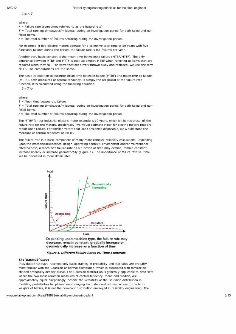
The failure rate is a basic component of many more complex reliability calculations. Depending

upon the mechanical/elect rical design, operating context, environment and/or maintenance

effectiveness, a machine’s failure rate as a function of time may decline, remain constant,

increase linearly or increase geometrically (Figure 1). The importance of failure rate vs. time

will be discussed in more detail later.

Figure 1. Different Failure Rates vs. Time Scenarios

The ‘Bathtub’ Curve

Individuals t hat have received only basic training in probability and stat istics are probably

most familiar with the Gaussian or normal distribution, which is associated with familiar bell-

shaped probability density curve. The Gaussian distribution is generally applicable to data sets

where the two most common measures of central tendency, mean and median, are

approximately equal. Surprisingly, despite the versatility of the Gaussian distribution in

modeling probabilities for phenomenon ranging from standardized test scores to the birth

weights of babies, it is not the dominant distribution employed in reliability engineering. The





Gaussian distribution has its place in evaluating the failure characteristics of machines with a

dominant failure mode, but the primary distribution employed in reliability engineering is the

exponential distribution.

When evaluating the reliability and failure characteristics of a machine, we must begin with

the much-maligned “bathtub” curve, which reflects the failure rate vs. t ime (Figure 2). In

concept, the bathtub curve effectively demonstrates a machine’s three basic failure rate

characteristics: declining, constant or increasing. Regrettably, the bathtub curve has been

harshly c riticized in the maintenance engineering literature because it fails to effec tively model

the c haracteristic failure rate for most machines in an industrial plant, which is generally true

at the macro level. Most machines spend their lives in the early life, or infant mortality, and/or

the constant failure rate regions of the bathtub curve. We rarely see systemic time-based

failures in industrial machines. Despite its limitations in modeling the failure rates of typical

industrial machines, the bathtub curve is a useful tool for explaining the basic concepts of

reliability engineering.

Figure 2. The Much-maligned ‘Bathtub’ Curve

The human body is an excellent example of a system that follows the bathtub curve. People,

and other organic species for that matter, tend to suffer a high failure rate (mortality) during

their first years of life, particularly the first few years, but the rate decreases as the child

grows older. Assuming a person reaches puberty and survives his or her teenage years, his or

her mortality rate becomes fairly constant and remains there until age (time) dependent

illnesses begin to increase the mortality rate (wearout). Numerous influences af fect mortality

rates, including prenatal care and mother’s nutrition, quality and availability of medical care,

environment and nutrition, lifestyle choices and, of course, genetic predisposition. These

factors can be metaphorically compared to factors that influence machine life. Design and

procurement is analogous to genetic predisposition; installation and commissioning is

analogous to prenatal care and mother’s nutrition; and lifestyle choices and availability of

medical care is analogous to maintenance effectiveness and proactive control over operating

conditions.

The exponential distribution

The exponential distribution, the most basic and widely used reliability prediction formula,

models machines with the constant failure rate, or the flat section of the bathtub curve. Most

industrial machines spend most of t heir lives in the c onstant failure rate, so it is widely

applicable. Below is the basic equation for est imating the reliability of a machine that follows

the exponential distribution, where the failure rate is constant as a function of time.

Where:

R(t) = Reliability estimate for a period of t ime, cycles, miles, etc . (t ).

e = Base of the natural logarithms (2.718281828)λ = Failure rate (1/MTBF, or 1/MTTF)

In our electric motor example, if you assume a constant failure rate the likelihood of running a

motor for six years without a failure, or t he projected reliability, is 55 percent . This is

calculated as follows:

R(6) = 2.718281828-(0.1* 6)

R(6) = 0.5488 = ~ 55%

In other words, aft er six years, about 45% of the population of identical motors operat ing in

an identical application can probabilistically be expected to fail. It is worth reiterating at this

point that these calculations project the probability for a population. Any given individual from

the population could fail on the first day of operation while another individual could last 30

years. That is the nature of probabilistic reliability projections.

A characteristic of the exponential distribution is the MTBF occurs at the point at which the





calculated reliability is 36.78%, or the point at which 63.22% of the machines have already

failed. In our motor example, after 10 years, 63.22% of the motors from a population of

identical motors serving in identical applications can be expected to fail. In other words, the

survival rate is 36.78% of the population.

We often speak of projected bearing life as the L10 life. This is the point in time at which 10%

of a population of bearings should be expected to fail (90% survival rate). In reality, only a

fraction of the bearings actually survive to the L10 point. We’ve come to accept that as the

objective life for a bearing when perhaps we should set our sights on the L63.22 point,

indicating that our bearings are lasting, on average, to projected MTBF – assuming, of course,

that the bearings follow the exponential distribution. We’ll discuss t hat issue later in the

Weibull analysis section of the article.

The probability density funct ion (pdf), or life distribution, is a mathematical equation that

approximates the failure frequency distribution. It is the pdf, or life frequency dist ribution,

that yields the familiar bell-shaped curve in the Gaussian, or normal, distribution. Below is the

pdf for the exponential distribution.

Where:

pdf(t) =Life frequency distribution for a given t ime (t)

e = Base of the natural logarithms (2.718281828)

λ = Failure rate (1/MTBF, or 1/MTTF)

In our elect ric motor example, the ac tual likelihood of failure at three years is c alculated as

follows: pdf(3) = 01. * 2.718281828-(0.1* 3)

pdf(3) = 0.1 * 0.7408

pdf(3) = .07408 = ~ 7.4%

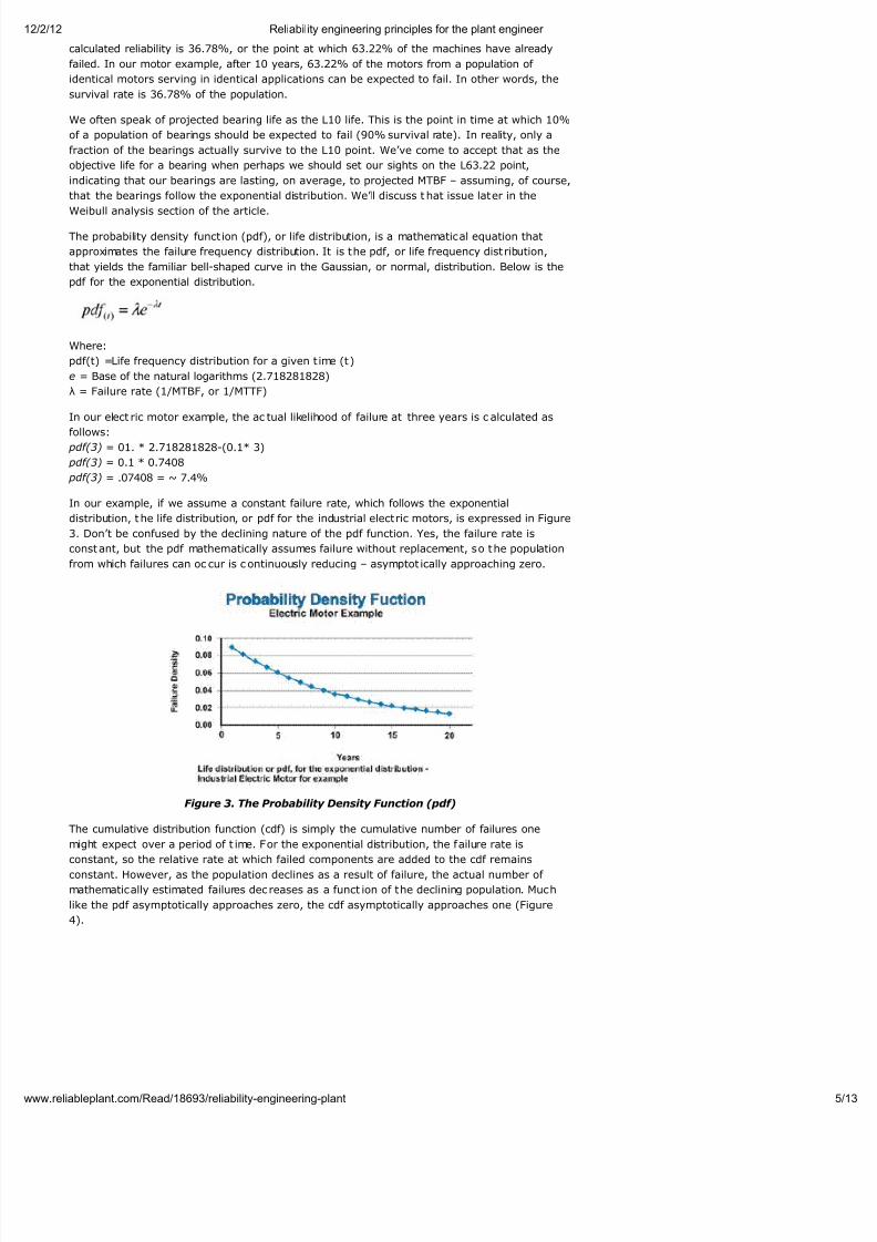
In our example, if we assume a constant failure rate, which follows the exponential

distribution, t he life distribution, or pdf for the industrial electric motors, is expressed in Figure

3. Don’t be confused by the declining nature of the pdf function. Yes, the failure rate is

constant, but the pdf mathematically assumes failure without replacement, so the population

from which failures can oc cur is continuously reducing – asymptot ically approaching zero.

Figure 3. The Probability Density Function (pdf)

The cumulative distribution function (cdf) is simply the cumulative number of failures one

might expect over a period of t ime. For the exponential distribution, the failure rate is

constant, so the relative rate at which failed components are added to the cdf remains

constant. However, as the population declines as a result of failure, the actual number of

mathematically estimated failures decreases as a funct ion of the declining population. Much

like the pdf asymptotically approaches zero, the cdf asymptotically approaches one (Figure

4).





Figure 4. Failure Rate and the Cumulative Distribution Function

The declining failure rate portion of the bathtub curve, which is often called the infant

mortality region, and the wear out region will be discussed in the following section addressing

the versatile Weibull distribution.

Weibull Distribution

Originally developed by Wallodi Weibull, a Swedish mathematician, Weibull analysis is easily the

most versatile distribution employed by reliability engineers. While it is called a distribution, it

is actually a tool that enables the reliability engineer to first characterize the probability

density function (failure frequency distribution) of a set of failure data to characterize the

failures as early life, constant (exponential) or wear out (Gaussian or log normal) by plotting

time to failure data on a special plotting paper with the log of the times/cycles/miles to failure

plotted a log scaled X-axis versus the cumulative percent of the population represented by

each failure on a log-log scaled Y-axis (Figure 5).

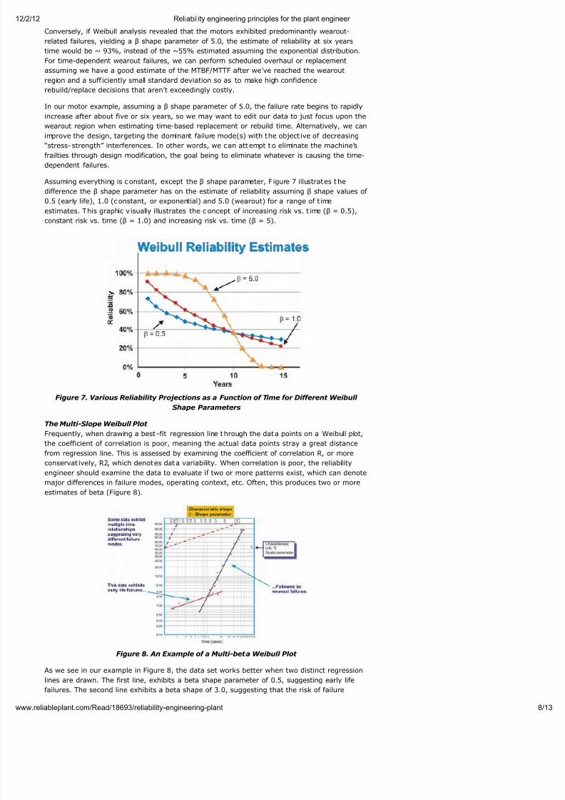
Figure 5. The Simple Weibull Plot – Annotated

Once plotted, the linear slope of the resultant curve is an important variable, called the shape

parameter, represented by â, which is used to adjust the exponential distribution to fit a wide

number of failure distributions. In general, if the â coefficient, or shape parameter, is less than

1.0, the distribution exhibits early life, or infant mortality failures. If the shape parameter

exceeds about 3.5, the data are time dependent and indicate wearout failures. This data set

typically assumes the Gaussian, or normal, distribution. As the â coefficient increases above ~

3.5, the bell-shaped distribution tightens, exhibiting increasing kurtosis (peakedness at the

top of the curve) and a smaller standard deviation. Many data sets will exhibit two or even

three distinct regions. It is common for reliability engineers to plot, for example, one curve

representing the shape parameter during run in and another curve to represent the constant

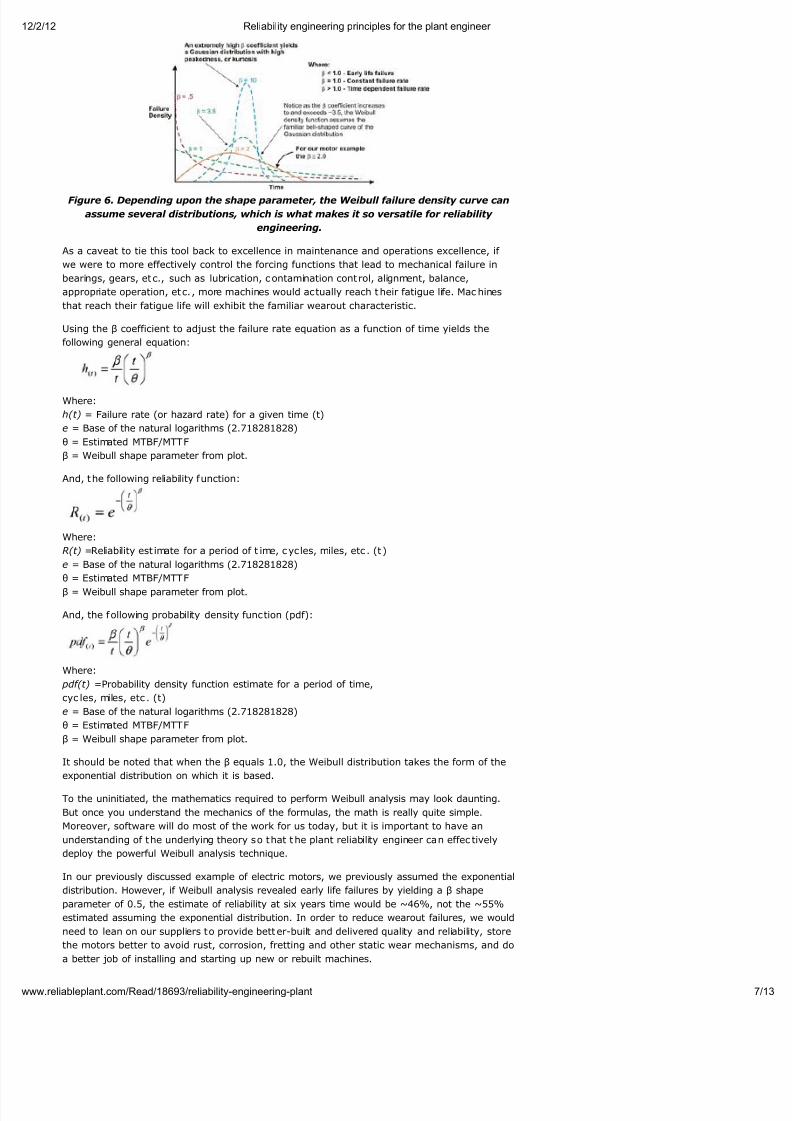
or gradually increasing failure rate. In some instances, a third distinct linear slope emerges toidentify a third shape, the wearout region. In these instances, the pdf of the failure data do in

fact assume the familiar bathtub curve shape (Figure 6). Most mechanical equipment used in

plants, however, exhibit an infant mortality region and a constant or gradually increasing

failure rate region. It is rare to see a curve representing wearout emerge. The characteristic

life, or η (lower case Greek “Eta”), is t he Weibull approximation of the MTBF. It is always the

function of time, miles or cycles where 63.21% of the units under evaluation have failed,

which is the MTBF/MTTF for the exponential distribution.





Figure 6. Depending upon the shape parameter, the Weibull failure density curve can

assume several distributions, which is what makes it so versatile for reliability

engineering.

As a caveat to tie this tool back to excellence in maintenance and operations excellence, if

we were to more effectively control the forcing functions that lead to mechanical failure in

bearings, gears, etc., such as lubrication, contamination control, alignment, balance,

appropriate operation, etc., more machines would actually reach their fatigue life. Machines

that reach their fatigue life will exhibit the familiar wearout characteristic.

Using the β coefficient to adjust the failure rate equation as a function of time yields the

following general equation:

Where:

h(t) = Failure rate (or hazard rate) for a given time (t)


θ = Estimated MTBF/MTTF

β = Weibull shape parameter from plot.

And, the following reliability function:

Where:

R(t) =Reliability est imate for a period of t ime, cycles, miles, etc . (t )




And, the following probability density function (pdf):

Where:

pdf(t) =Probability density function estimate for a period of time,

cyc les, miles, etc . (t)




It should be noted that when the β equals 1.0, the Weibull distribution takes the form of the

exponential distribution on which it is based.

To the uninitiated, the mathematics required to perform Weibull analysis may look daunting.

But once you understand the mechanics of the formulas, the math is really quite simple.

Moreover, software will do most of the work for us today, but it is important to have an

understanding of the underlying theory so that t he plant reliability engineer can effec tively

deploy the powerful Weibull analysis technique.

In our previously discussed example of electric motors, we previously assumed the exponential

distribution. However, if Weibull analysis revealed early life failures by yielding a β shape

parameter of 0.5, the estimate of reliability at six years time would be ~46%, not the ~55%

estimated assuming the exponential distribution. In order to reduce wearout failures, we would

need to lean on our suppliers to provide bett er-built and delivered quality and reliability, store

the motors better to avoid rust, corrosion, fretting and other static wear mechanisms, and do

a better job of installing and starting up new or rebuilt machines.





increases as a function of time. It is common for complex equipment, particularly mechanical

equipment, to experience “run-in” failures when new or recent ly rebuilt. As such, t he risk of

failure is highest just following initial start-up. Once the system works through its run-in

period, which can take minutes, hours, days, weeks, months or years, depending upon the

system type, the system enters a different risk pattern. In this example, the system enters a

period where the risk of failure increases as a function of time once the system exits its run-in

period.

The multi-beta offers the reliability engineer a more precise est imate of risk as a funct ion of

time. Armed with this knowledge, he or she is better posit ioned to take mitigating act ions. For

example, during the early life period, we’d be inclined to improve the precision with which we

manufacture/rebuild, install and start-up. Moreover, we might add monitoring techniques

and/or increase our monitoring frequency during the high risk period. Following the run-in

period, we might introduce monitoring tec hniques that are targeted at the t ime-dependent

wearout failures that are believed to affect the system, increase monitoring frequency

acc ordingly or schedule “hard-time” preventive maintenance ac tions in some cases.

Estimating System Reliability

Once the reliability of components or machines has been established relative t o the operating

context and required mission time, plant engineers must assess the reliability of a system or

process. Again, for the sake of brevity and simplicity, we’ll discuss system reliability estimates

for series, parallel and shared-load redundant system (r/n systems).

Series Systems

Before discussing series systems, we should discuss reliability block diagrams. Not a

complicated tool to use, reliability block diagrams simply map a process from start to finish.

For a series system, Subsystem A is followed by Subsystem B and so forth. In the series

system, the ability to employ Subsystem B depends upon the operating state of Subsystem A.

If Subsystem A is not operating, the system is down regardless of the condition of Subsystem

B (Figure 9).

To calculate the system reliability for a serial process, you only need to multiply the estimated

reliability of Subsystem A at time (t) by t he est imated reliability of Subsystem B at t ime (t).

The basic equation for calculating the system reliability of a simple series system is:

Where:

Rs(t) – System reliability for given time (t)

R1-n(t) – Subsystem or sub-funct ion reliability for given time (t )

So, for a simple system with three subsystems, or sub-functions, each having an estimated

reliability of 0.90 (90%) at time (t), the system reliability is calculated as 0.90 X 0.90 X 0.90 =

0.729, or about 73%.

Figure 9. Simple Serial System

Parallel Systems

Often, design engineers will incorporate redundancy into critical machines. Reliability engineers

call these parallel systems. These systems may be designed as active parallel systems or

standby parallel systems. The block diagram for a simple two component parallel system is

shown in Figure 10.

Figure 10. Simple parallel system – the system reliability is increased to 99% due to

the redundancy.





To calculate the reliability of an active parallel system, where both machines are running, use

the following simple equation:

Where:

Rs(t) – System reliability for given time (t)

R1-n(t) – Subsystem or sub-funct ion reliability for given time (t )

The simple parallel system in our example with two components in parallel, each having a

reliability of 0.90, has a total system reliability of 1 – (0.1 X 0.1) = 0.99. So, the system

reliability was significantly improved.

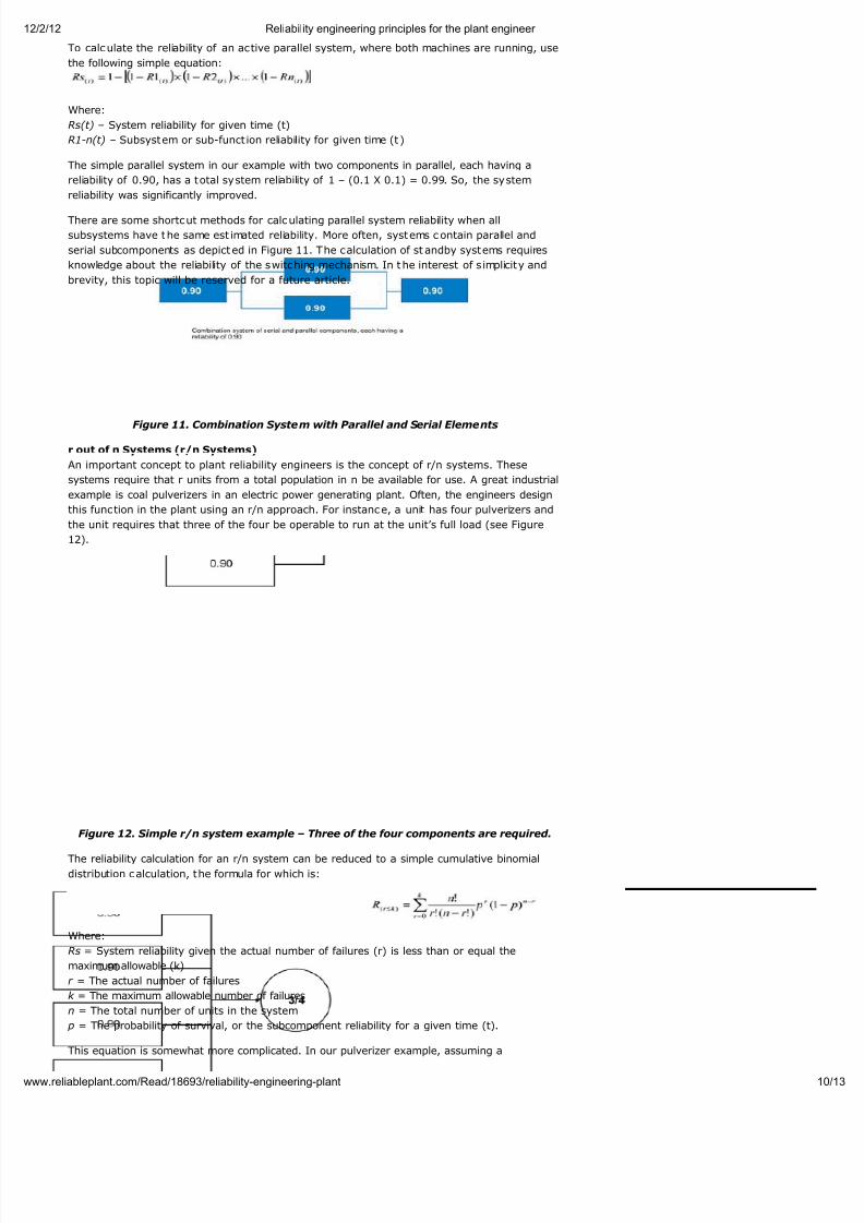
There are some shortcut methods for calculating parallel system reliability when all

subsystems have the same est imated reliability. More often, systems contain parallel and

serial subcomponents as depict ed in Figure 11. The calculation of st andby systems requires

knowledge about the reliability of the switching mechanism. In the interest of simplicity and

brevity, this topic will be reserved for a future article.

Figure 11. Combination System with Parallel and Serial Elements

r out of n Systems (r/n Systems)

An important concept to plant reliability engineers is the concept of r/n systems. These

systems require that r units from a total population in n be available for use. A great industrial

example is coal pulverizers in an electric power generating plant. Often, the engineers design

this function in the plant using an r/n approach. For instance, a unit has four pulverizers and

the unit requires that three of the four be operable to run at the unit’s full load (see Figure

12).

Figure 12. Simple r/n system example – Three of the four components are required.

The reliability calculation for an r/n system can be reduced to a simple cumulative binomialdistribution calculation, the formula for which is:

Where:

Rs = System reliability given the actual number of failures (r) is less than or equal the

maximum allowable (k)

r = The actual number of failures

k = The maximum allowable number of failures

n = The total number of units in the system

p = The probability of survival, or the subcomponent reliability for a given time (t).

This equation is somewhat more complicated. In our pulverizer example, assuming a





Bayesian applications of reliability engineering methods

Stress-strength interference analysis

Testing options and their applicability to plant reliability engineering

Reliability growth strategies and management

More detailed understanding of field data collect ion.

Most important, spend time learning how to apply reliability engineering methods to plant

reliability problems. If your interest in reliability engineering methods is high, I encourage you

to pursue professional certification by t he American Society for Quality as a reliability engineer

(CRE).

References

Troyer, D. (2006) Strategic Plant Reliability Management Course Book, Noria Publishing, Tulsa,

Oklahoma.

Bernowski, K (1997) “Safety in the Skies,” Quality Progress, January.

Dovich, R. (1990) Reliability Statist ics, ASQ Quality Press, Milwaukee, WI.

Krishnamoorthi, K.S. (1992) Reliability Methods for Engineers, ASQ Quality Press, Milwaukee,

WI.

MIL Standard 721

IEC Standard 300-3-3

DOE Standard NE-1004-92

Appendix: Select reliability engineering terms from MIL STD 721Availability – A measure of the degree to which an item is in the operable and committable

state at the start of the mission, when the mission is called for at an unknown state.

Capability – A measure of the ability of an item to achieve mission object ives given the

conditions during the mission.

Dependability – A measure of the degree to which an item is operable and capable of

performing its required function at any (random) time during a specified mission profile, given

the availability at the start of the mission.

Failure – The event, or inoperable state, in which an item, or part of an item, does not, or

would not, perform as previously specified.

Failure, dependent – Failure which is caused by the failure of an associated item(s). Not

independent.

Failure, independent – Failure which occurs without being caused by the failure of any other

item. Not dependent.

Failure mechanism – The physical, chemical, electrical, thermal or other process which

results in failure.

Failure mode – The consequence of the mechanism through which the failure occurs, i.e.

short, open, fracture, excessive wear.

Failure, random – Failure whose oc currence is predictable only in the probabilistic or

statistical sense. This applies to all distributions.

Failure rate – The total number of failures within an item population, divided by the t otal

number of life units expended by that population, during a particular measurement interval

under stated conditions.

Maintainability – The measure of the ability of an item to be retained or restored to specified

condition when maintenance is performed by personnel having specified skill levels, using

prescribed procedures and resources, at each prescribed level of maintenance and repair.

Maintenance, corrective – All actions performed, as a result of failure, to restore an item to

a specified condition. Corrective maintenance can include any or all of the following steps:

localization, isolation, disassembly, interchange, reassembly, alignment and checkout.

Maintenance, preventive – All actions performed in an attempt to retain an item in a

specified condition by providing systematic inspection, detection and prevention of incipient

failures.

Mean time between failure (MTBF) – A basic measure of reliability for repairable items: the

mean number of life units during which all parts of the item perform within their specified




limits, during a particular measurement interval under stated conditions.

Mean time to failure (MTTF) – A basic measure of reliability for non-repairable items: The

mean number of life units during which all parts of the item perform within their specified

limits, during a particular measurement interval under stated conditions.

Mean time to repair (MTTR) – A basic measure of maintainability: the sum of correct ive

maintenance t imes at any specified level of repair, divided by the total number of failures

within an item repaired at that level, during a particular interval under stated conditions.

Mission reliability – The ability of an item to perform its required functions for t he duration

of specified mission profile.

Reliability – (1) The duration or probability of failure-free performance under stated

conditions. (2) The probability that an item can perform its intended function for a specified

interval under stated conditions. For non-redundant items this is t he equivalent t o definition

(1). For redundant items, this is the definition of mission reliability.

About the author:

Drew D. Troyer is a champion of effective reliability management and passionate about helping

companies f ind hidden profits inside their plants. As a highly sought consultant to Fortune 500

manufacturing firms, award-winning columnist and teacher, he understands both management

expectations and plant-floor realities. Troyer is a Certified Reliability Engineer (CRE), a

Certified Maintenance and Reliability Professional (CMRP), and chairs t he standards committee

of the Society for Maintenance and Reliability Professionals (SMRP). Contact Drew at 800-

597-5460.

Related ArticlesThe Link between Reliability and Safety

Employ Smart Redundancy for Reliability

Using Overall Equipment Effectiveness

Follow-up is Key for Greater Efficiency

Get a FREE copy of 6 Essentials for

Effective Procedure-based

Maintenance when you sign up for our free

Reliable Plant weekly email updates.

Email:

Lubrication Program TransformationServicesDiscover how Noria can tranform your lubrication

program to best practices quickly and efficiently.

Click Here

Begin a Free Subscription TodayMachinery Lubrication magazine delivers

unbiased advice for improving lubrication

practices and keeping critical equipment

running at peak performance.

Click Here

Services Subscribe | Contact Us | Privacy Policy | RSS | Advertise

Quick Links Home | Buyers Guide | Glossary | Events | Bookstore | Newsletters | Blogs | Browse Topics

© NORIA CORPORATION MACHINERY LUBRICATION | RELIABLE PLANT

reliability engineering principles for the plant engineer

Documents