reliability growth testing effectiveness - reliability analytics toolkit
TRANSCRIPT

R A O C - 1 R - 8 4 - 2 0
In-Hob^o Report Januctry i?84
RELIABILITY GROWTH TESTING EFFECTIVENESS
AD-A141 232
Preston R. MacDiarmid and Seymour F. Morrlf
> -D _ O CJ>
LxJ
APPROVED FOR PUBLIC RELEASE; DISTRIBUTION UNLIMITED
DTIC ELECTEI M A r 2 1 1984
ROME AIR DEVELOPMENT CENTER Air Force Systems Command
Griffiss Air Force Base, NY 13441
8 4 0 5 21 0 0 7

This report has been reviewed by the RADC Public Affairs Office (PA) and
is releascble to the National Technical Information Service (NTIS). At RTIS
it will be releasable to the general public, including foreign nations.
RADC-TR-84-20 h3S been reviewed and is approved for publication.
^ f APPROVED:
ANTHOOT J . FEDUCCIA
Chief, Systems Reliability & Engineering Branch Reliability & Compatibility Division
APPROVED:
W . S. TUTHILL, Colonel, USAF Chief, Reliability & Compatibility Division
FOR THE COMMANDER:
JOHN A . RITZ
Acting Chief, Plans Ofiice
If your address has changed or it; you wish to be removed from the RADC mailing
Xi3t r or if the addressee is no longer employed by your organization, please
notify RADC (RBER) Griffiss AFB F? 13441. This will assist us in maintaining
a current miD/ir-^ lis".
Do r^t return cop ies ol" t.i. is reuort unless contractual obligations or notices
on a specific oo-'u ac-ut -!-<?<;uirt
,s that it be returned.

V V v v
UNCLASSIFIED
REPORT OOCUMEHTA.TION P A G E R K A D I N S T R U C T I O N S B E F O R E C O M P L E T I N G F O R M
1. R E P O R T N U M B E R 2 . O O V T A C C E S S I O N NO.
RADC-TR-84-20 / f b ~ A X ^ i
J. R E C I P I E N T ' S C A T A L O O N U M B E R
4 u 4. T I T L E (and Subttth)
RELIABILITY GROWTH TESTING
EFFECTIVENESS
S. T Y P E O F R E P O R T T P E R I O D C O V E R E D
In-House Report
4. T I T L E (and Subttth)
RELIABILITY GROWTH TESTING
EFFECTIVENESS 6. P E R F O R M I N G 0 ^ 0 . R E P O R T N U M B E R
N/A 7. AUTHO«F»;
Preston R. MacDiarmid
Seymour F. Morris
*. C O N T R A C T O R G R A N T N U M B E R S
N/A
». P E R F O R M I N G O R G A N I Z A T I O N N A M E AH 5 AOORESS
Rome Air Development Center (RBER)
Griffiss AFB NY 13441
10. P R O G R A M E L E M E N T . P R O J E C T , TASK A R E A A WORK UNIT N U M B E R S
62702F
23380289
1 1. CONTROLLING OFFICE NAME ANC. ADDRESS
Rome Air Development Center (RBER) Griffiss AFB NY 13441
12. REPORT DATE
January 1984
1 1. CONTROLLING OFFICE NAME ANC. ADDRESS
Rome Air Development Center (RBER) Griffiss AFB NY 13441
13. NUMBER OF PAGES
172 1«. MONITORING AGENCY NAME 4 ADDRESSF// dlllirtnt IrOM Controlling Olflca)
Same
IT. SECURITY CLASS. Co 1 thli report)
UNCLASSIFIED
1«. MONITORING AGENCY NAME 4 ADDRESSF// dlllirtnt IrOM Controlling Olflca)
Same IS«. DECLASSIFICATION / DOWN GRADING N / A
S C H e 0 u L E
1«. DISTRIBUTION STATEMENT (ot Ihlm Report)
Approved for public release; distribution unlimited
17. DISTRIBUTION STATEMENT (ol th* mbitrme: anlartd In Block 10, It dllftrmni /ROOI Kmpo'.)
Same
18. SUPPLEMENTARY NOTES
None
1 9 . K E Y w o n c s (Continue on ttvort* j I d * II n i c » i > r a n d Idt.'tlly by bljck ni.oi>«j •
Reliability r Reliability Growth Test Analyze and Fix
Duane F - f v
2 0 . A B S T R A C T (Contlnum o n rmvormm ltd* II ntcm»*mry mid Identify by block n u n t x r ;
This in-house report documents the results of an RADC Systems Reliability and Engineering Branch in-house study on reliability growth testing. The study involved examination of DoD policy regarding this form of testing, an extensive literature search on techniques and applications as well as consultation with Air Force reliability experts on the subject. The results address a general overview of models and techniques applied with particular attention to unique approaches found in the literature. Numerous current
DD 1473 E D I T I O N O F I NOW «5 IS O B S O L E T E UNCLASSIFIED
S E C U R I T Y C L A S S I F I C A T I O N O F THIS P A G E FWRIWL Dmlm Entttod)
*
w • V
•
. I . > - I

UNCLASSIFIED 1KCUWTY CLASSIFICATION OF THI» PAOKflWi— O f Btm^)
i&nd past Air Force applications are cited indicating the range of possible approaches. The report concludes by addressing many of the questions regarding reliability growth testing Repressed by those skeptical of it.
4
DTIC ELECTE M A Y 2 1 1994
9
. %«• * & *
tV Accession '/or
NTIS CRA&I DTIC TAB 1'nnnnouiicrd Q J u:: 11 £ i f •"> t i o u
fiv _ _
Distribution/
Availability Codes
Avail and/or
Dist Special

s w ^ if. w. tr. w .
TABLE OF CONTENTS
SECTION
1,0
2.0
3.0
4.0
PAGE
Objective 1
Approach 1
2.1 Jssues 2
Reliability Growth Testing Terminology 5
3.1 Reliability Testing 5
3.2 Growth and Failures 6
3.3 Failure Reporting and Corrective Action System 8
(FRACAS)
3.4 Reliability Growth Limiting Values 10
3.5 Reliability Growth in Management 11
3.6 Reliability Growth vs Other Reliability Tasks 11
3.7 No-Growth Growth 12
0 Dnl i -.x; 1 rvuti.41. M-I .. •! «« «. II • o i\gi i uu iiivjr uiunbii n ijuuiiucpi IUM9 IC.
DoD Policy on Reliability Growth Testing 13
4.1 Standards 13
4.2 Development Process 16
4.2.1 Reliability Development Phases 17
4.3 Tailoring Tasks 18
4.4 Direction 19
4.4.1 DoD Directive 5000.40: "Reliability and 24
Maintainability" (8 Jul 80)
4.4.2 AFR 800-18: "Air Force Reliability and 25
Maintainability Program" (15 Jun 82)
•v"
'a'--':
.V. v . v .
- \"V ".• '• •!•

TABLE 01- CONTENTS
SECTION PAGE
4.4.3 MIL-STD-785B: "Reliability Programs for 28
Systems and Equipment Development and
Production" (15 Sep 8C)
4.4.4 MIL-STD-781C: "Reliability Design 36
Qualification and Production Acceptance
Tests: Exponential Distribution"
(21 Oct 77) (Currently Under Revision to
MII.-STD-781D, See paragraph 4.4.5)
4.4.5 rtIL-STD-781D (31 Dsc 80 Draft) 36
4.4.6 MIL-STD-1635(EC): "Reliability Growth 37
Testing" (3 Feb 73)
4.4.7 MIL-STD-20b8: "Reliability Development 39
Testing" (21 Mar 77)
4.4.8 MIL-NDBK-139: "Reliability Growth 40
Management" (13 Feb 81)
5.0 Reliability Growth Analysis 43
5.1 Reliability Growth Model Types 43
5.2 Reliability Growth Models 47
5.2.1 The Duane Model 47
2.2 The AMSAA Model 53
5.,:,3 Duane-vs-AMSAA Model 57
5.2.4 Other Models 59
5.2.r Nonre'evant Failures 65

TABLE OF CONTENTS
SECTION PAGE
6.0 Reliability Growth Management Techniques 66
6.1 Reliability Growth Test or Not 67
6.2 Planning for Reliability Growth 72
6.2.1 Initial Reliability 77
6.2.2 The Growth Rate (a) 77
6.3 Reliability Growth Test Time 83
6.3.1 Reliability Growth Test Time Estimation 84
for a System
6.3.2 Allocating Reliability Growth Test Time to 86
Subsystems
6.3.3 Test Time Example 88
6.3.4 Planning Test Time 93
6.4 The Exponential Law for the Appearance of 93
Systematic Failures
6.5 Tracking Techniques 96
6.6 Confidence Levels 99
6.7 Cost of a Growth Program 100
7.0 Reliability Growth Application Experience 104
7.1 Current Air Force Applications 104
7.1.1 HAVE CLEAR (Formerly SEEK TALK) 105
7.1.2 SACDIN 106
7.1.3 AFSATCUM 106
7.1.4 JTIDS 107
iii

TABLE 01- CONTENTS
SECTION
7.1.5 Simulator SPO
7.1.6 F-16
7.1.7 Bl-B
7.1.8 AMRAAM
7.1.9 B-52 OAS
7.1.10 AWACS
7.1.11 AN/ARC-164
7.2 Program Application Summary
8.0 Conclusions
8.1 Suimiary of Conclusions
APPENDIX A Test Time Tables
APPENDIX B Bibliography
PAGE
107
107
108
108
109
109
110
110
111
128
A-l
B-l
s"
V
'. v V
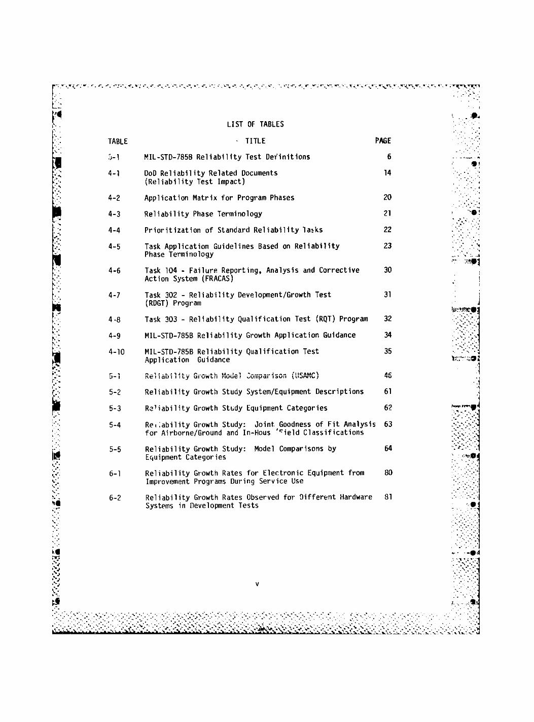
LIST OF TABLES
• TITLE PAGE
MIL-STD-785B Reliability Test Definitions 6
DoD Reliability Related Documents 14 (Reliability Test Impact)
Application Matrix for Program Phases 20
Reliability Phase Terminology 21
Prioritization of Standard Reliability Tasks 22
Task Application Guidelines Based on Reliability 23 Phase Terminology
Task 104 - Failure Reporting, Analysis and Corrective 30 Action System (FRACAS)
Task 302 - Reliability Development/Growth Test 31 (RDGT) Program
Task 303 - Reliability Qualification Test (RQT) Program 32
MIL-STD-785B Reliability Growth Application Guidance 34
MIL-STD-785B Reliability Qualification Test 35 Application Guidance
n . u . L j u i . . r» .4.L •> .'ilCAurM AC
R\E I I O L H M I Y U I U W L . I I N U U C R W U M P A I I S U I I ivtjra-ii>/ I U
Reliability Growth Study System/Equipment Descriptions 61
Ratability Growth Study Equipment Categories 62
Reliability Growth Study: Joint. Goodness of Fit Analysis 63 for Airborne/Ground and In-Hous '
rield Classifications
Reliability Growth Study: Model Comparisons by 64 Equipment Categories
Reliability Growth Rates for Electronic Equipment from 80 Improvement Programs During Service Use
Reliability Growth Rates Observed for Different Hardware 81 Systems in Development Tests

v-3
n I
V / . -
V.N' ••M
TABLE TITLE PAGE
6-3 Examples of Reliability Growth Rates Unc'sr RIW Programs n?
6-4 Comparison of Reliability Growth Rates 83
6-5 Variations of Reconmended Test Times Presented in the 84 Literature
6-6 Subsystems and Their Required M T B F S 87
6-7 Tost Time In Terms of Multiples of the Required MTPF 87
6-8 Initial Growth Test Data 88
6-9 Relhbility Attributes and Application Levels 101
6-10 Reliability Attribute levels for a Given State 102
7-1 Air Force Reliability Growth Applications 105
8-i Questions Regarding RDGT Implementation 113
••mi
• -1
'"V-*
liWI
V V • 1
y . ^ f ' m *
VI

LIST OF FIGURES
FIGURE TITLE PAGE
3.1 Categorization of Defects 7
3.2 Failure Reporting and Corrective Action System 9
3.3 Endless Burn-In Concept 10
4.1 Reliability Document Impact on RADC 15
4.2 System Development Pharss 16
5.1 Failure Rate Versus Cumulative Operating Hours for 47 Duane's Original Data
5.2 Duane Plot for Reliability Growth of an Airborne 49 Radar
5.3 Duane P t Showing the Initial "Hook" During the 51 Early Ti:ne Period
5.4 Initial Hook in Bathtub Cu~ve Showing an Initially 51 low Failure Rate (High MTBF)
5.3 Linear/Staircase Plot of R0G7 Test Data S2
6.1 Options Available to a Program Mai lger for a Fixed 70
Reliability Test Time
6.2 Reliability Tests as a Function of Contract Type 71
6.3 Planned Reliability Growth (Continuous) 73
6.4 Planned Reliability &, owth (Phase-uy-Phase) 73
6.5 Reliability Growth Process Showing a Decrease in 76 Reliability ("DIPS") at Certain Program Milestones
6.6 Different Ways of Reaching the Sv.„ie MTBF Goal 86
6.7 Plotted Data for Test Time Calculation Example 90
6.8 Exponential Law for the Appearance of Systematic 94 Failures
6.9 Percent Increase in Acquisition Cost-vs-Normalized MTBF 102
v n
L .

. - • - • - * . - w • » « »• i * \r" i."*' l
FIGURE TITLE
6.10 Reliability Task Cost Relationships
8.1 Comparison of Cumulative Life Cycle Cost; With and Without Specified Reliability Growth Test Requirements
PAGE
103
115
•V-v-i
IV.V. k\ . . K"
' I
m .•r-ci
r -r • ,1
-VV ' '
i •
k'-V-
Vlll
m 4
Y - ' H . „• I "
1
v v,
• .1

I*0 Objective: The use of reliability growth testing and test-analyze-
and-f'x (TAAF) testing has become widespread within the Department of
Defense as a complement to and substitute for formal reliability qualifi-
cation testing. Many different models, tools and techniques for their use
have been presented in the literature, military standards and handbooks.
Still, many reliability experts within DoD question the utility and cost
effectiveness of reliability growth testing and describe it as rewarding
contractors for sloppy initial designs. The objective of this study was to
tully investigate the subject of reliability growth testing to enable a
better understanding by reliability engineers as wall as to present guid-
ance for its potential application in the development of Air Force systems.
2.0 Approach: The approach used in performing the in-house study
included the following:
A. Existing Department of Defense and Air Force regulations, direc-
tives, standards, handbooks and policies were reviewed to determine their
impact on the forms of reliability testing under study.
B. A literature search regarding reliability growth testing and
test-analyze-and-fix testing was performed to determine how requirements
have been/are being implemented, what management and analysis techniques
have been developed and what the results have been of the application of
those techniques.
1

C. Various reliability experts (government/industry) were consul :ed
to benefit from their experience in applying reliability growth testiig.
Opinions and data were sought with respect to applying reliability growth
and TAAF testing.
D. DoD research and development data bases were searched to deter-
mine what R&D study efforts are currently under way regarding these forms
of reliability testing.
E. The results of the above four tasks were reviewed and analyzed by
an objective RADC team of experienced reliability engineers and conclu-
sions were developed.
2.1 Issues: While reliability growth testing is being applied widely in
DoD systems development, there are a number of questions that are often
expressed by those skeptical of its effectiveness which can be summarized
as follows:
Who pays for the reliability growth testing (RDG7)? Does the
government end up paying mors?
Does RDGT allow DoD contractors to "get away with" a sloppy init-
ial design because they can fix it later at the government's
expense?

Should reliability growth testing be dedicated or Integrated?
When should a reliability growth test begin?
Should reliability growth be planned for beyond the FSED phase?
Should the equipment operate at the fully specified performance
level prior to the start of RDGT?
Should all development programs have some sort of reliability
growth testing?
How does the applicability of reliability growth testing vary
with the following points of a development program?
a. Co.-nplexity of equipment and its challenge to the state-of-
the-art.
b. Operational environment
c. Quantity of equipment to be produced
What growth model(s) should be used?
What starting points and growth rates should be used for
planning?
3

How n&'cft tesv time (and calendar time) will be required to conduct
U u testing?
toiien will corrective actions be implemented?
How will failures be counted?
Will there be an accept/reject criteria?
Should the contractor be responsible for intermediate milestones?
Can/should growth testing be incentivized?
Does the type of contract affect RDGT decisions?
What is adequate time for verifying a design fix?
What is the relationship between an RQT and RDGT?
Who will do the growth tracking? How and to whom will the
results/status be reported?
How much validity/confidence should be placed on the numerical
results of RDGT?

Based on the research conducted, an a .tempt will be made to answer many of
these questions 1n the remainder of the report. The results of the study
are organized as follows 1n the remainder of the report.
3.0 Reliability Growth Testing Terminology
4.0 DoD Policy on Reliability Growth Testing
5.0 Reliability Growth Analysis
6.0 Reliability Growth Management Techniques
7.0 Reliability Growth Application Experience
8.0 Conclusions
3.0 Reliability Growth Testing Terminology
3.1 Reliability Testing: The use and misuse of many reliability testing
terms necessitates inclusion of the Table 3-1 definitions. It should be
noted that Reliability Growth Testing (RGT) and Reliability Develop-
ment/Growth Testing (RDGT) are used synonymously in this report. Test-
Analyze-and-Fix (TAAF) is the process by which reliability growth is
achieved and, in itself, does not necessarily include the structured
planning and tracking associated with an RG1. MIL-STD-785B considers the
Reliability Development/Growth Test as an engineering test while the other
two forms of reliability testing are considered accounting tests. Before
considering the applicability of reliability growth testing, some prelimi-
nary concepts need to be addressed:

TABLE 3-1: MIL-STD-785B RELIABILITY TEST DEFINITIONS
Environmental Stress Screening (ESS): A series of tests conducted under environmental stresses to disclose weak parts and workman-ship defects for correction.
Reliability Development/Growth Test (RDGT): A series of tests conducted to disclose deficiencies and to verify that corrective actions will prevent recurrence in the operational inventory. (Also known as "TAAF" testing)
Reliability Qualification Test (RQT): A test conducted under spe-cified conditions, by, or on behalf of, the government, using items representative of the approved production configuration, to determine compliance with specified reliability requirements as a basis for production approval. (Also known as a "Reliability Demonstration," or "Design Approval" test.)
Production Reliability Acceptance Test (PRAT): A test conducted under specified conditions, by, or on behalf of, the government, using delivered or deliverable production items, to determine the producer's compliance with specified reliability requirements.
3.2 Growth and Failures: PH Mead (Ref 5) states that there are three
distinct ways in which reliability can grow:
"Growth Mode 1. By operating each equipment (or portion of it) to
expose and eliminate rogue components or manufacturing errors.
Growth Mode 2. By familiarization, increased operator skill and
general "settling down" in manufacturing, use and servicing.
Growth Mode 3. By discovering and correcting errors or weaknesses in
design- manufacturing or related procedures."
Reliability of electronic equipment can improve both at the collective and
individual equipment level. Burn-in improves the reliability of the
equipment subjected to it while design changes improve (or degrade) the
reliability of all equipment subject to the changes. Each of the three
growth or evolution modes can be made more effective by planned activities.
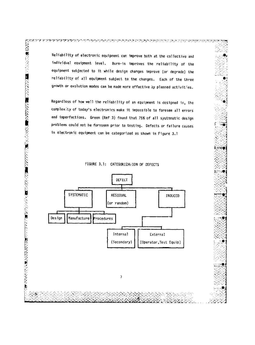
Regardless of how well the reliability of an equipment is designed in, the
complexity of today's electronics make it impossible to foresee all errors
and imperfections. Green (Ref 3) found that 75% of all systematic design
problems could not be foreseen prior to testing. Defects or failure causes
in electronic equipment can be categorized as shown in Figure 3.1
FIGURE 3.1: CATEGORIZATION OF DEFECTS
7

Head defined the three failure classes as:
A. Systematic - repetitive (or from their nature liable to be
repetitive).
B. Irxluced - Due to accident from causes internal or external to the
equipment.
C. Rasidual - Neither of the above.
A constant review of defects is necessary to ensure that random and induced
categorized events aren't alibis for performing no corrective action. He
found that an exponential law applied to the appearance of systematic
failures in complex airborne equipment. Most authors speak of reliability
growth testing as a means of eliminating these systematic failures.
3.3 Failure Reporting and Corrective Action System (FRACAS): A well
accepted military reliability program task is a closed loop FRACA system as
shown in Figure 3.2. The reliability growth test can be thought of as a
better controlled and more structured form of a FRACAS system.
8

y ^ y v ^ ^ V J m ^ y * •T* L"* tf"* f 'J-* 'tT* V 'r* « J*'.. "J 'V 'I TT -y-^m^w-^-w -
FIGURE 3.2: FAILURE REPORTING AND CORRECTIVE ACTION SYSTEM
FAILURE OBSERVATION
RELIABILITY DEVELOPMENT
TEST
INCORPORATE CORRECTIVE ACTION INTO DEVELOP EQUIP
FAILURE DOCUMENTATION
r 3 INCORPORATE CORRECTIVE ACTiON INTO PRODUCTION
YES DETERMINE EFFECTIVENESS
Or CORRECTIVE ACTION
NO DETERMINE ] CORRECTIVE
INCORPORATE CORRECTIVE ACTiON INTO PRODUCTION
DETERMINE EFFECTIVENESS
Or CORRECTIVE ACTION
ACTION 1
1
ESTABLISH ROOT CAUSE
SUSPECT ITEM REPLACEMENT
FAILURE ANALYSIS
Almost all programs recognize the payoff of such a task. In fact, it could
be argued that any system or equipment development, military or commer-
cial, must have some ^ort of FRACAS system to be successful over the long
term. Differences among FRACAS programs are in the depth of failure
analysis and in the implementation of corrective action (the degree to
which the system is "closed loop"). Whether quantified or planned for, a
FRACAS is a cost effective process which results in improved system
reliability.

3.4 Reliability Growth Limiting Values: Bezat (Ref 6) postulated the
sources of growth to be two categories, (1) reliability growth due to
conscious corrective action, and, (?) "endless burn-in" maturing factor.
He showed that growth continues to a limiting reliability level even with-
out further design corrective activity. The idea of "endless burn-1n"
means that "infant mortality" is a misnomer and that the magnitude of its
effects extend far out in life. The effect was categorized as follows:
"Endless Burn-In includes all the intangible maturity factors associated
with undocumented improvements in test, repair, build processes, and con-
trol of environment/application to original objectives/1 Bezat states
that the instantaneous failure rate of an LRU includes a residual component
which becomes significant only when the average age of the LRU's becomes
about 2500 hours (Fig 3.3).
FIGURE 3.3: ENDLESS BURN-IN CONCEPT

^ - w_-* * * i - ir^ - » " * - i - 1
» • r - J " v' - . - I - I •
V*
3.5 Reliability Growth 1n Management: If the premise of reliability
Improvement through design change 1s believed, the question becomes how
effective 1s the process and how much resources are required to meet the
reliability requirements? Meade (Ref 8) said: "Reliability growth man-
agement facilitates early warning by helping a manager 1n at least four
ways: First 1s the preparation of planned, time phased profiles of relia-
bility growth. Next, the methodology can be used to assess reliability
progress against „h1s plan. Third, projections of reliability trends can
be developed. Finally, the methodology can be used as a powerful planning
tool for determining the time and resources needed for the test phases of a
reliability program and 1n evaluating the impact of limitations and
changes in the program." In the context of reliability growth in this
report, it is important to emphasize that growth results from redesign
effort that eliminates failure sources that were discovered through analy-
sis of test results. An important aiscinction to be made is that in the
burn-in of an item, defect'»e parts are replaced with good parts of the
same desig;i resulting in an improved reliability of the one unit being
burned-in. Redesign to eliminate failure sources involves changing the
design configuration of c.ll units, not just the one under test.
3.6 Reliability Growth vs Other Reliability Tasks: Mead (Ref 5)
described as a necor^ity for a successful growth process "starting with a
healthy plant" which results from the other reliability program tasks. The
reliability growth management process provides an orderly way to control
the development process, surface problems and redirect assets.
11
• . *
•• J
• • • "VR
• ^ >
\ —• ,
-•>'
. - . •*
" .V
^V-V.
*»V-V
A .
" - • ?

3.7 No-Grcwth Growth: Clark (Ref 42) cautioned against the misuse of
reliability growth concepts by indicating cose histories which had been
previously portrayed as reliability growth in the literature that really
weren't. In his work he referred to situations where growth was portrayed
by using reliability demonstration data and individual equipment burn-iri
data as "no-growth growth." These were misapplications of growth manage-
ment and he cautioned, "to effect a growth in inherent reliability, one or
more of tne basic design or process parameters (number and types of compon-
ent parts, their material quality and stress levels and structural and
thermal characteristics) must be improved." An example of no-growth
growth would be the purging of systematic failures from reliability demon-
stration test data to show what the system reliability could be if a
perfect fix could be found for these problems. Unless the fixes are
actually implemented and proven, you will have a case of no-growth growth.
3.8 Reliability Growth Misconceptions: In order to further clarify reli-
ability growth it is important to point out the following misconceptions
regarding it:
A. Reliability growth is a naturally occurring phenomenon in elec-
tronic equipment. (It is not)
B. Reliability growth occurs as a natural course of events after a
system is introduced into the operational inventory. (It does not)
12

C. Equipment burn-in to remove infant mortality type failures causes
reliability growth. (It does not, except for that particular equipment)
D. Replacing early equipment failures with good parts to repair the
observed weaknesses causes reliability growth. (It does not)
E. Reliability predictions that improve with mere detailed design
disclosure reflect reliability growth. (They do not)
In the context of this report, reliability growth is the result of the
iterative process of sample testing; identification of design, part and
workmanship defects; and correction of the causes of these defects. The
basic equipment design establishes the point from which reliability growth
starts and the upper bound on potential reliability.
4.0 DoD Policy on Reliability Growth Testing
4.1 Standards: Reliability as an engineering discipline is controlled by
a series of directives, regulations, standards, handbooks and policies
within the DoD acquisition and development arena. Some of these are
triservice (apply to all DoD components) others are uniquely designeu for
one or more services' use. Table 4-1 is a representation of these docu-
ments. Figure 4.1 shows a hierarchy of how RADC, in particular, is
effected by these reliability documents on development and acquisition
programs.
13

TABLE l-l: DOD RELIABILITY RELATED DOCUMENTS (RELIABILITY TEST IMPACT)
NUMBER TITLE
DoD 5000.40 Reliability and Maintainability (8 July 1980)
AIR 800-•18 Air Force Reliability and Maintainability Pro-
gram (15 June 1982)
ML--STD- 785B Reliability Program for Systems and Equipment
Development and Production (15 September 1980)
MIL--STD-
CO Reliability Design, Qualification and Produc-
tion Acceptance Tests: Exponential Distribu-
tion (21 October 1977)
r1IL-•STD- 721C Definitions of Terms for Reliability and Main-
tainability (12 June 1982)
MIL-•STD- 1635 Reliability Growth Testing (3 February 1978)
' J T 1 R I I L -
R R N •O 1 U - CUDO Reliability Development Tests (21 March 19/7)
MIL- HDBK -189 Reliability Growth Management (13 February
1981)
14

FIGURE. 4.1: RELIABILITY DOCUMENT IMPACT OT3 RADC
DoD 5000.40
AFR 800-18
s • * - 1 . " 1
1 -v JL-. --"- i
.-- ."j
. • , • . - .
••V-V-'.S
y y
MIL-STD-781
uri c m i>*ir I'llL-OIL/- ID JO
MIL-STD-2068
MIL-HDBK-189
AFSC SUPPLEMENT TO
AFR 800-18
1 MIL-STD--785
MIL-STD-1629
MIL-STD-756
MIL-HDBK-217
I TAILORING
MIL-STD-721
MIL-STD-965
fc -
.v.-v^ •y\..\v-»V" ,*J
•". '..vy, --vNr." v * >\-'
DEVELOPMENT
PROCESS
v •« '
15
•'•...•vV-.C-"'--"' • t ».a«
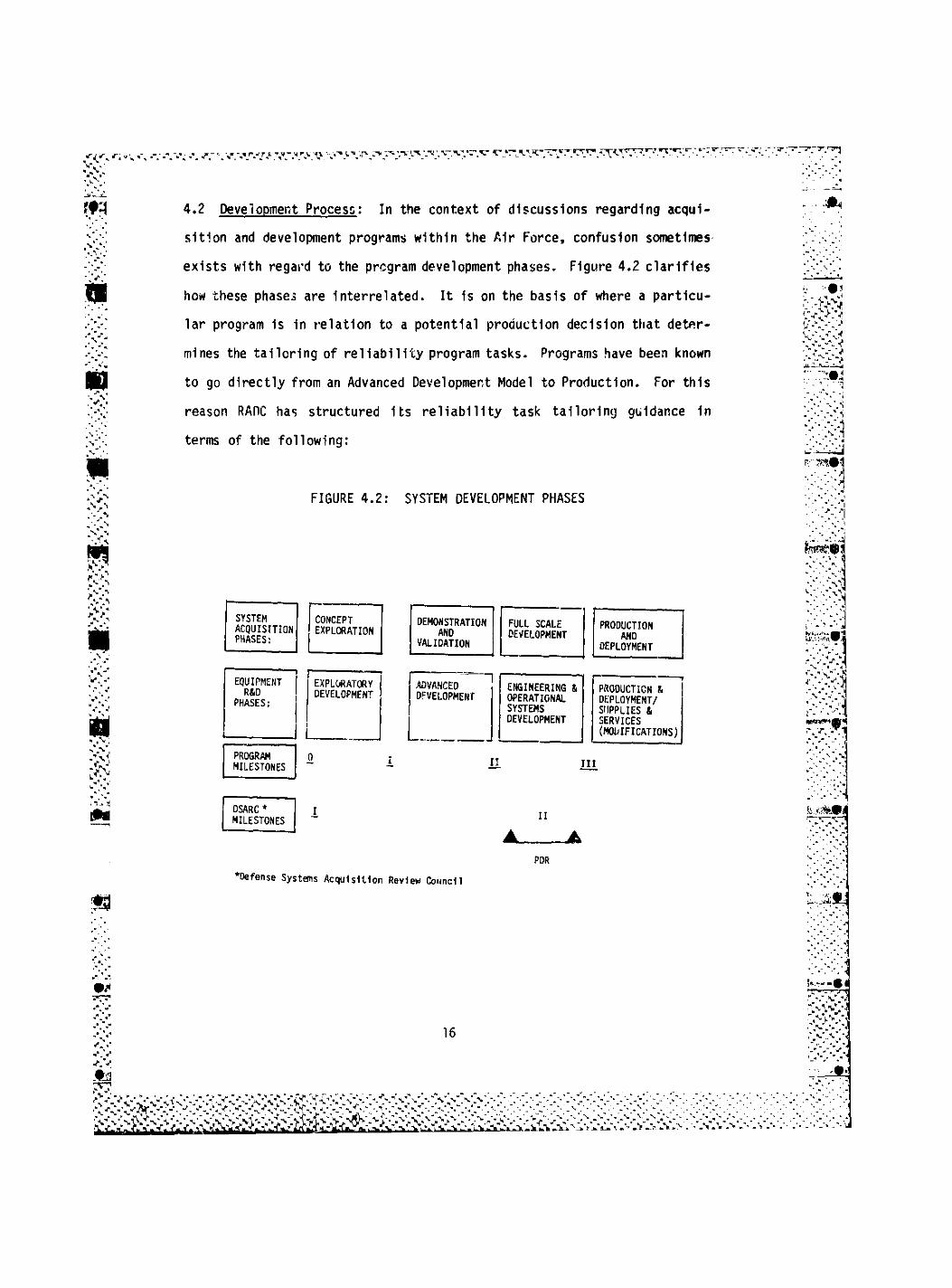
4.2 Development Process: In the context of discussions regarding acqui-
sition and development programs within the A1r Force, confusion sometimes
exists with regard to the program development phases. Figure 4.2 clarifies
how these phases are Interrelated. It 1s on the basis of where a particu-
lar program is 1n relation to a potential production decision that deter-
mines the tailoring of reliability program tasks. Programs have been known
to go directly from an Advanced Development Model to Production. For this
reason RADC has structured Its reliability task tailoring guidance 1n
terms of the following:
FIGURE 4.2: SYSTEM DEVELOPMENT PHASES
SYSTEM CONCEPT ACQUISITION EXPLORATION PHASES:
EXPLORATION
EQUIPMENT EXPLORATORY R&D DEVELOPMENT
PHASES:
PROGRAM 0 MILESTONES
DSARC * I MILESTONES
DEMONSTRATION AND
VALIDATION
•Defense Systems Acquisition Review Council
FULL SCALE DEVELOPMENT
PRODUCTION AND
DEPLOYMENT
ADVANCED DFVELOPMENT
ENGINEERING OPERATIONAL SYSTEMS DEVELOPMENT
PRODUCTION k DEPLOYMENT/ SUPPLIES & SERVICES (MODIFICATIONS)
II III
II
PDR
16

4.2.1 Reliability Development Phases:
A. Pre-Reliability Phase: Those early phases in a development pro-
cess where no structured reliabilty tasks are appropriate.
B. Reliability Study Phase' This early phase has reliability acti-
vities related to trade studies accessing the reliability potential of
various system configurations.
C. Reliability Design/Analysis Phase: This phase begins the sig-
nificant application of reliability engineering tasks to the system devel-
opment. Activities will provide the framework for the next phase (usually
FSED). It is not the last development phase before a potential production
decision.
D. Reliability Definition and Demonstration Phase: This phase is
the final development process prior to a production decision. Reliability
engineering is a major part of this phase's development process. Reliabi-
lity quantitative parameters are specified, predicted and demonstrated.
E. Reliability Assurance Phase: This phase is the build, test and
deliver of the reliability designed in during prior development. Reliabi-
lity activities are devoted mainly to "assurance" type tasks such as envi-
ronmental stress screening and production reliability acceptance testing.
17

Table 4-2 has beeh extracted from MIL-STD-785B "Reliability Program For
Systems and Equipment Development and Production" to show how particular
reliability tasks are to be tailored for a particular development phase.
The terminology used for phase definitions of Table 4-2 are thac of AFR
800-1 "Major System Acquisitions." Many RADC development programs are
covered by the AFR "80" series regulations with such phases as "exploratory
development," "advanced development," "engineering development" and
others. In some instances phases are omitted from the development cycle.
A program can transition directly from an advanced development model (ADM)
to production. Therefore, the key to effective implementation of reliabi-
lity requirements and tasks is not in tying them to development phase names
but in defining them in terms of how close the development phase is to a
production decision which must include reliability consideration. Table
4-3 indicates the general reliability considerations as a function of
reliability design phase terminology.
4.3 Tailoring Tasks: While MIL-STD-785B recommends reliability tasks for
the various phases of development, as indicated by Table 4-2, it is impor-
tant to note that each program is different in terms of funding/schedule,
equipment performance requirements, challenge to the state-of-the-art, and
personnel and contractors involved. Therefore, a "boiler plate" approach
to reliability is never the correct approach. Raccntly, RADC's reliabi-
lity experts prioritized standard reliability tasks in accordance with
their payoff for varying environments and development phases. Table 4-4
shows the results. These results were based on a mix of the "80" series
18

and "800" series AF regulations terminology in that the phases ADM-FSED-
PROD are considered. After recognizing (as previously pointed out) that
there are cases where an ADM goes directly to production without further
development, RADC formulated reliability task application guidelines based
on the reliability phase terminology. These results are represented by
Table 4-5. In line with all recent reliability literature, the emphasis 1s
placed on "up front" reliability engineering tasks, rather than reliabi-
lity accounting tasks.
4.4 Direction: While tailoring is key to successful cost effective reli-
ability accomplishment, certain reliability aspects are required by relia-
bility directives, regulations and standards. The following paragraphs
address how the documents of Table 4-1 relate to reliability growth and
TAAF testing.
19

TABLE 4-2: APPLICATION MATRIX FOR PROGRAM PHASES
TAS:: TITLE TASK TYPE
PROGRAM PHASE TAS:: TITLE TASK
TYPE CONCEPT VALID FSED PROD
101 RELIABILITY PROGRAM PLAN MGT S S G G
102 MONITOR/CONTROL OF SUBCONTRACTORS AND SUPPLIERS
MGT s S <*, G
103 PROGRAM REVIEWS MGT s S(2) G(2) 6(2)
104 FAILURE REPORTING, ANALYSIS. AND CORRECTIVE ACTION SYSTEM (FRACAS)
ENG NA S G G
105 FAILURE REVIEW BOARD (FRB) MGT NA S(2) G G
201 RELIABILITY MODELING ENG S S(2) G(2) GC(2)
202 RELIABILITY ALLOCATIONS ACC S G G GC
203 RELIABILITY PREDICTIONS ACC S S(2) G(2) GC(2)
204 FAILURE MODES, EFFECTS, AND CRITICALITY ANALYSTS (FRTECA)
ENG S 0)(2)
G
(!)(?) GC
(D(2)
205 SNEAK CIRCUIT ANALYSIS (SCA) ENG NA NA 6(1) GC(1)
206 ELECTRONICS PARTS/CIRCUITS TOLERANCE ANALYSIS
ENG NA NA G GC
207 PARTS PROGRAM ENG S
(2)0)
G
(2) G (2)
208 RELIABILITY CRITICAL ITEMS MGT S<1) S(L) G r
209 EFFECTS OF FUNCTIONAL TESTING, STORAGE, HANDLING, PACKAGING, TRANSPORTATION, AND MAINTENANCE
ENG NA S(l) G GC
301 ENVIRONMENTAL SFRESS SCREENING (ESS) ENG NA S G G
302 RELIABILITY DEVELOPMENT/GROWTH TESTING
ENG NA 3(2) 6(2) NA
303 RELIABILITY QUALIFICATION TEST (RQT) PROGRAM
ACC NA S(2) 6(2) 6(2)
304 PRODUCTION RELIABILITY ACCEPTANCE ACCEPTANCE TEST (PRAT) PROGRAM
ACC N" NA S G (2)13)
CODE DEFINITIONS
TASK TYPE:
ACC - RELIABILITY ACCOUNTING
ENG - RELIABILITY ENGINEERING
MGT - MANAGEMENT
PROGRAM PHASE:
S - SELECTIVE APPLICABLE
G - GENERALLY APPLICABLE
GC - GENERALLY APPLICABLE TO DESIGN CHArtGES ONLY
NA - f'.OT APPLICABLE
(1) - REQUIRES CONSIDERABLE INTERPRETATION OK INTENT TO BE COST EFFECTIVE
(2) - MIL-STD-785 IS NOT THE PRIMARY IMPLEMENTATION REQUIREMENT. OTHER MIL-STDS OR STATEMENT OF WORK REQUIREMENTS MUST BE INCLUDED TO DEFINE THE REQUIREMENTS.
20

TABLE 4-3: RELIABILITY PHASE TERMINOLOGY
PRE R/M R/M STUDY R/M DESIGN & ANALYSTS
R/M DEFINITION & DEMONSTRATION
R/M ASSURANCE
o Research 0 R/M Trade vs 0 Realistic Range o Firm Quantitative 0 F<rm Quantitative Op and Support of RIM Values RIM Requirements RIM Requirements
o Mission Area Constraints Analysis 0 R&M Predictions o Formal RIM 0 Sample Tests Analysis
0 Similar System Testing o R/M Deficiencies Measurement 0 R*M Analyses 0 Deficiencies
Identified of Test Data o Growth, TAAF Resolved 0 Risk Assessment 4 CERT
o No Quantitative c Design Deficiencies 0 ESS (Parts/Equip) or Qualitative 0 Quantitative Identified o MIL-STD-470 R/M Requirements R/M Objectives & 785 Programs 0 Failure Free
Established 0 Update of Scrsenlr.g Operational RIM o Design Review
0 Quantitative Requirements Requirements o Repair Level Not Required 0 Risk Assessment Analysis
0 Tailored RIM o Independent RIM Quantitative Review Requirements
o Deficiencies 0 No Formal RIM Identified &
Testing Corrected
21

V„'<
I i & V.v
I N > .
m
£
A'' V .
KX-.-
•a P7?
.»v
TABLE 4-4: PRIORITIZATION OF STANDARD RELIABILITY TAoKS
RELIABILITY TASK GROUND AVIONICS SPACE RELIABILITY TASK
ADM FSED PROD ADM FSED PROD ADM FSED PROD
Establish Valid Numerical Rqm't 1 1
Parts Selection & Control 1 2 1 2 1 1
Derating 3 3 2 3 2 2
FMEA X 5 4 4 3
R Model Prediction & Allocation 2 4 4 5 3 5
FRACAS 4 5 2 X 8 2 X 6 3
RQT 6 7
ESS 3 3 2
PRAT 4 4
QA X 1 1 1
"OGT X X 6 4
mak Analysis X X X X X
/1 c 'WS A X
Failure Review Board X X X
Cri ^al Items X X X X X X X X
Subcontractor Control X X X X X X
0. _ ,izat1on X X
Thermal Management & Analysis X X 3 X 5 X
Storage Effects X X X X X X
NOTE: Numbered tasks are essential; for a giver phase the lower the number the greater the payoff.
1 « Greatest payoff X » Should be considered

w-.-v-' y ' - y
" > M < < ' S . < IL- * r j t t a t S J m
S •> »
j / *
v.- vv Irr \
i,r i 7 r
TABLE 4-5: TASK APPLICATION GUIDELINES BASED ON RELIABILITY PHASE TERMINOLOGY
^ / r V 7 »-
fry
PRE RELIABILITY RELIABILITY DESIGN AND ANALYSIS PHASE RELIABILITY DEFINITION RELIABILITY RELIABILITY STUDY AND DEMONSTRATION PHASE ASSURANCE
RESEARCH PAPER LIMITED LIMITED QT" HI POTENTIAL C O W OFF MILITARIZED COMM OFF PRODUCTION PRODUCT POTENTIAL FIELD USE (FURTHER THE SHELF THE SHEuF
DEVELOPMENT)
o Not o Trade Study 0 Model 0 Model 0 Model 0 Model 0 Model 0 Model 0 FRACAS Applicable for several 0 Allocation 0 Allocation 0 Allocation 0 Allocation 0 Allocation 0 AT location (with CA)
configurations 0 Prediction 0 Prediction 0 Prediction 0 Prediction 0 Prediction 0 Prediction 0 ESS o Prediction Tvpe B/E/C Type B/C Type A/B/C/ Type B/C/D Type A/C Type B/C/D (Env Stress
Type C/D/E 0 FRACAS 0 FRACAS 0 FRACAS 0 FRACAS 0 FRACAS 0 FRACAS Screen) (w/o CA) (w/o CA) (with CA) (with CA) (with CA) (with CA) 0 PRAT
0 Reviews 0 Reviews 0 Reviews 0 Reviews 0 Reviews 0 Reviews (Prod Rel) 0 Rel Select 0 Rel Select 0 Rel Select c Rel Select 0 Subcontract 0 Subcontract 0 £CP Review
Criteria Criteria Criteria Criteria Control Control (Eng Change 0 Verification 0 Rel Design(2) t> Rel Des1gn(3) 0 Rel Des1gn(l) 0 Rel Des1gn(3) Proposals)
0 Verification by Analysis - Parts - Parts - Pa<-ts - Parts by Analysis - Thermal - Thermal - Thermal - Thermal 0 Subcontractor
0 In-House 0 Verification - Derating • De: :ing • Derating - Derating 0 Critical Rel Data Hi Risk Test 0 Verification 0 Verification 0 RQT 0 RQT Items Collection/ 0 In-House by Analysis b.' Analysis 0 FMECA c FRB Analysis Rel Data
by Analysis 0 Storage/ 0 Storage/
Collection/ 0 FMEA 0 Verification 0 Critical Handling Handling Analysis 0 TAAF Hi tlsk Test Items 0 FMECA 0 SCA
0 Rel 0es1t|n(2) 0 RQT 0 Growth 0 Program - Parts Test Plar - Therma" 0 Program 0 SCA - Derating Plan 0 ESS - Derating
0 Storage/ Handling
0 SCA 0 ESS
PREDICTION TYPE A - Stress Analysis B - Part Type/Count C - Vendor Data D - Similar Equipment E - Procuring Activity
Reliability Design (1) - Full MILSPEC Parts, Stringent Thermal Design and Derating (2) - Substitution of Lower Quality
Parts Permissible With Minimum Screens, Reduced Thermal Design and Derating (3) - Modified Design Areas Only
FRACAS (CA) - Corrective Actions Implemented
A >'. •'. •'•
s
c.\
.'/l" - V V v , v>.
Jr S
• TT '.• V V
" * - - » ik-.
•

4.4.1 DoD Directive 5000.40 "Reliabi 11 and Maintainability" (8 Jul
80): This directive requires a "balanced mix" of reliability engineering
and accounting tasks tailored for maximum efficiency. Under the reliabi-
lity engineering policy, reliability growth testing is listed as a design
fundamental to "disclose design deficiencies and to verify the effective-
ness of corrective action0 "
The di °ctive further states that "require-
ments and achievements for each applicable system R&M parameter shall be
numerically traceable: (a) through all phases of the system life cycle,
v ' ' * • w
•'
reliability engineering task by stating:
"R&M growth is required during full scale development, concurrent de-
velopment and production (where concurrency is approved), and during
initial deployment. Predicted R&M growth shall be stated as a series
each of these phases."
C W 24
-- ' u
•'.•J
..." It emphasizes the importance of reliability growth as a high payoff I--' . .
•-v-vo v* >.'
^ v - w i
V V • .
."-V w
[yS^ of intermediate milestones, with associated goals and thresholds, for •'< "S
"A. A period of testing shall be scheduled in conjunction with -y-y
each intermediate milestone The purpose of these tests shall be •
to find design deficiencies and manufacturing defects. A block
of time and resources shall be scheduled for the correction of I V V , i Ktd deficiencies and defects found by each period of testing, to ;
prevent their recurrence in the operational inventory. Adirsinis- ^"ySo
trative delay of R&M engineering change proposals shall be -y;"
minimized.
&
. . .

B. The differences between required values for system R&M para-
meters shall be used to concentrate R&M engineering effort where
it is needed (for example, enhance mission reliability by cor-
recting mission-critical failures; reduce maintenance manpower
st by correcting any failures that occur frequently).
C. Approved R&M growth shall be assessed and enforced. Enfor-
cement of intermediate R&M goals ^hill be left to the acquiring
activity. Failure to achieve an intermediate R&M threshold is a
projected threshold breach, and if it occurs, an immediate review
by the program decision authority is required."
With regard to reliability demonstration, the directive says "R&M demon-
stration, qualification tests and acceptance tests shall be tailored for
effectiveness and efficiency (maximum return on cost arid schedule invest-
ment) in terms of management information they provide." Reliability
growth testing is considered an engineering task while reliability demon-
stration testing is considered an accounting task. Accounting tasks
measure reliability (demonstrate a value) while engineering tasks improve
reliability.
4.4.2 AFR 800-18: "Air Force Reliability and Maintainability Program
(15 June 1982): This document is intended to revise the previous AF
Regulation 80-5 to comply with DoD 5000.40. Requirements of DoD 5000.40
are restated with phrases such as "...it is necessary to address R&M
thresholds at each program decision milestone. These thresholds will be
derived from mature system requirements," and "each R&M program will
25
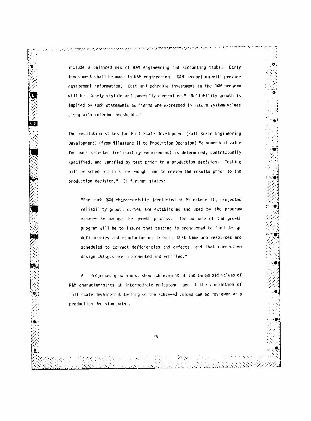
include a balanced mix of R&M engineering and accounting tasks. Early
investment shall be made in R&M engineering. R&M accounting will provide
management information. Cost and schedule investment in the R&M proyirnm
will be clearly visible and carefully controlled." Reliability growth Is
implied by such statements as "terms are expressed in mature system values
along with interim thresholds."
The regulation states for Full Scale Development (Full Scale Engineering
Development) (from Milestone II to Production Decision) "a numerical value
for each selected (reliability requirement) is determined, contractually
specified, and verified by test prior to a production decision. Testing
will be scheduled to allow enough time to review the results prior to the
production decision." It further states:
"For each R&M characteristic identified at Milestone II, projected
reliability growth curves are established and used by the program
manager to manage the growth process. The purpose of the yrowtii
program will be to insure that testing is programmed to find design
deficiencies and manufacturing defects, that time and resources are
scheduled to correct deficiencies and defects, and that corrective
design changes are implemented and verified."
A, Projected growth must show achievement of the threshold values of
R&M characteristics at intermediate milestones and at the completion of
full scale development testing so the achieved values can be reviewed at a
production decision point.
26

B. Growth curves shall not be used to predict achievement of
requirements in the production phase unless either concurrent development
and production are specifically authorized, or funds have been identified
to correct specific R&M deficiencies.
C. A projected growth curve is established for each contractually
specified parameter. These curves must show adequate progress to achieve
the specified value before commencement of reliability qualification
testing.
D. Use test-analyze-and-fix (TAAF) techniques to accomplish neces-
sary reliability growth. Actual growth will be tracked through monitoring
of functional, environmental, and evaluation testing conducted during
development. However, specific reliability growth tests, such as Combined
Environmental Reliability Test (CERT), should be conducted when compatible
with the ove> ill program schedule." (This applies also for concurrent FSD
and production).
The regulation defines the FSD program by:
"The FSD program is intended to mature the system R&M characteristics
as soon as possible by finding and correcting design deficiencies,
reducing producibi1ity risks and by identifying and pursuing R&M
improvement opportunities. To do this:
27

A. The approved design approach shall be matured through devel-
opment testing of equipment and the incorporation of specific
design Improvements.
B. Ihe maturation process shall be monitored through growth
tracking and design review ev luations."
4.4.3 MIL-STD-785B "Reliabi 1 it.y Programs for Systems and Equipment
Development and Production" (15 Sep 80): This revision of the main DoD
reliability standard Dresents a "shopping list" of reliability tasks to be
tailored to a given application. The recommendations given for task appli-
cation were already cited in Table 4-2. Increased emphasis (over MIL-STD-
785A) is placed on reliability engineering tasks and tests with the thrust
toward prevention, detection, and correction of design deficiencies, weak
parts and workmanship defects. This standard stresses reliability
pnainpprinn-.
"Reliability Engineering. Tasks shall focus ori the prevention,
detection, and correction of reliability design deficiencies, weak
parts, and workmanship defects. Reliability engineering shall be an
integral part of the item design process, including design changes.
The means by which reliability engineering contributes to the design,
and the level of authority and constraints on this engineering dis-
cipline, shall be identified in the reliability program plan. An
28

efficient reliability program shall stress early investment in relia-
bility engineering tasks to avoid subsequent rosts and schedule
delays."
With respect to demonstration of contractual reliability requirements
(electronics), the standard states "conformance to the minimum acceptable
MTBF requirement shall be demonstrated by tests selected from MIL-STD-781,
or alternative specified by the PA (procuring activity)." Reproduced for
completeness as Tables 4-6, 4-7 and 4-8 are respectively: Task 104,
"Failure Reporting, Analysis, and Corrective Action System"; Task 302,
"Reliability Development/Growth Test (RDGT) Program"; Task 303, "Reliabi-
lity Qualification Test (RQT) Program."
29

TABLE 4-6: TASK 104 - FAILURE REPORTING, ANALYSIS AND CORRECTIVE ACTION SYSTEM (FRACAS)
104.1 Purpose. The purpose of task 104 1s to establish a closed loop failure reporting system, procedures for analysis of failures to determine cause, ahd documentation for record-ing corrective action tai.'; .
104.2 Task Description
104.2.1 The contractor shall have a closed loop system that collects, analyzes, and records failures tha*. occur for specified levels of assembly prior to acceptance of the hardware by the procuring activity. The contractor's existing data collection, analysis and corrective action system shall be utilized, with modification only as necessary to meet the requirements specified by the PA.
104.2.? Procedures for inflating failure reports, the- analysis of failures, feedback of correctna action Into the design, manufacturing and test processes shall be Identified. Flow dlajram(s) depicting failed hardware and data flow shall also be documented. The analysis of failures shall establish and categorize the cause of failure.
104.2.3 The closed loop system shall Include provisions to assure that effective corrective actions are taken on a timfely basis by a follow-up audit that reviews all open failure reports, failure analyses, and corrective action suspense dates, and the reporting of delin-quencies to management. The failure cause for each failure shall be clearly stated.
104.2.4 When applicable, the method of establishing and recording operating time, or cycles, on equipments shall be clearly defined.
104.2.5 The contractor's closed loop failure reporting system data shall be transcribed to Government forms only 1f specifically required by the procuring activity.
104.3 Details to be Specified by the PA (reference 1.2.2.1)
104.3.1 Details to be specified in the SOW shall include the following, as applicable:
a. Identification of the extent to which the contractor's FRACAS must be compa-tible with PA's data system.
(R) b. Identification of level of assembly for failure reporting.
c. Definitions for failure cause categories.
d. Identification of logistic support requirements for LSAR.
e. Delivery identification of any data item required.
30

TABLE 4-7: TASK 302 - RELIABILITY DEVELOPMENT/GROWTH (RDGT) PROGRAM
302.1 Purpose. The purpose of task 302 Is to conduct pre-qual1f1cat1on testing (also known as TAAF) to provide a basis for resolving the majority of reliability problems early In the development phase, and Incorporating corrective action to preclude recurrence, prior to the start of production.
302.2 Task Description
302.2.1 A reliability development/jrowth test (TAAF test) shall be conducted for the purpose of enhancing system reliability through the Identification, analysis, and correction of failures and the verification of the corrective action effectiveness. Here repair of the test item does not constitute corrective action.
302.2.1.1 To enhance mission ^liability, correctly action shall be focused on mission-critical failure modes. To enhance basic reliability, corrective action shall be focused on the most frequent failure modes regardless of their mission criticality. These efforts shall be balanced to meet predicted growth for both parameters.
302.2.1.2 Growth testing will emphasize performance monitoring, failure detection, fail-ure analysis, and the incorporation and verification of design corrections to prevent recur-rence of failures.
302.2.2 A TAAF test plan shall be prepared and shall Include the following, subject to PA approval prior to Initiation of testing:
a. Test objectives and requirements, including the selected growth model and growth rate and the rationale for both selections.
b. Identification of the equipment to be tested and the number of test items of each equipment.
c. Test conditions, environmental, operational and performance profiles, and the duty cycle.
d. Test schedules expressed in calendar time and item life units, including the test milestones and tesc program review schedule.
e. Test ground rules, chargeability criteria and Interface boundaries.
f. Test facility and equipment descriptions and requirements.
g. Procedures and timing for corrective actions.
h. Blocks of time and resources designated for the incorporation of design corrections.
1. Data collection and recording requirements,
j. FRACAS.
k. Government furnished property requirements.
1. Description of preventive maintenance to be acconvllshed during test,
m. Final disposition of test Items,
n. Any other relevant considerations.
302.2.3 As specified by the procuring activity, the TAAF test plan shall be submitted to the procuring activity for its review and approval. This plan, as approved, shall be Incorpor-ated into the contract and shall become the basis for contractual compliance.
302.3 Details io be Specified by the PA (reference 1.2.2.1)
302.3.1 Details to be specified in the SOW shall Include the following, as applicable:
(R) a. Imposition of task 104 as a requisite task.
(RJ b. Identification of a 1ife/mission/environmental profile to represent equipment usage in service.
c. Identification of equipment and quantity to be used for reliability devel-opment/growth testing.
d. Delivery identification of any data items required.
" 31

TASK 4-8: TASK 303 - RELIABILITY QUALIFICATION TEST (RQT) PROGRAM
303.1 Purpose. The purpose of task 303 1s to determine that the specified reliability requirements have been achieved.
303.2 Task Description
303.2.1 Reliability qualification tests shall be conducted on equipments which shall be Identified by the PA and which shall be representative of the approved production config-uration. The relalbillty qualification testing may be integrated with the overall sys-tem/equipment qualification testing, when practicable, for cost-effectiveness; the RQT plan shall so Indicate in this case. The PA shall retain the right to disapprove the test failure relevancy and chargeabliity determinations for the reliability demonstrations.
303.2.2 An RQT plan sha1! be prepared in accordance with the requirements of MIL-STD-781, or
alternative approved by the PA, and shall include the following, subject to PA approval prior to initiation of testing:
a. Test objectives and selection rationale.
b. Identification of the equipment to be tested (with identification of the com-puter programs to be used for the test, 1f applicable) and the number of test items of each equipment.
c. Test duration and the appropriate test plan and test environments. The test plan and test environments (if life/mission profiles are not specified by the PA) shall be derived from MIL-STD-781. If it 1s deemed that alternative procedures are more appropriate, prior PA approval shall be requested with sufficient selection rationale to permit procuring activity evaluation.
d. A test schedule that is reasonable and feasible, permits testing of equipment which are representative of the approved production configuration, and allows sufficient time, as specified 1n the contract, for PA review and approval of each test procedure and test setup.
303.2.3 Detailed test procedures shall be prapared for the tests that are included in the RQT plan.
303.2.4 As specified by the procuring activity, the RQT plan and test procedures shall be submitted to the procuring activity for Its review and approval. These documents, as approved, shall be incorporated into the contract and shall become the basis for contractual compliance.
303.3 Details to be Specified by the PA (reference 1.2.2.1)
303.3.1 Details to be specified in the SOW shall include the following, as applicable:
(R) a. Identification of equipment to be used for reliability qualification testing.
(R) b Identification of MIL-STD-781, MIL-STD-105 or alternative procedures to be used for conducting the RQT (I.e., test plan, test conditions, etc.).
c. Identification of a life/mission/envlronme.ital profile to represent equipment usage 1n service.
d. Logistic support coordinated reporting requirements for LSAR.
e. Delivery identification of any data items required.
32

The standard cites three objectives of a reliability test program as:
A. Disclose deficiencies in item design, material and workmanship.
B. Provide measured reliability data as input for estimates of oper-
ational readiness, mission success, maintenance manpower cost and logis-
tics support cost.
C. Determine compliance with quantitative reliability requirements.
This is the priority order of the objectives to be met subject to cost and
schedule constraints. The previously mentioned tasks (302 and 303) along
with Task 301, "Environmental Stress Screening" and Task 304, "Production
Reliability Acceptance Testing" are the elements of a reliability test
program to be tailored to accomplish the above objectives. The standard
says "a properly balanced reliability program will emphasize ESS and RDGT,
and limit, but not eliminate* RQT and PRAT,"
This is in line with emphasis on engineering tasks and "up front" reliabi-
lity spending. Integrated testing is stressed with environmental tests
(MIL-STD-810) considered as the early portion of RDGT. With regard to the
use of ESS and RDGT as methods of determining contractual compliance, the
standard states: "ESS and RDGT must not include accept/reject criteria
that penalizes the contractor in proportion to the number of failures he
finds, because this would be contrary to the purpose of the testing so
these tests must not use statistical test plans that establish such
33

criteria. RQT and PRAT must, provide a clearly defined basis for determin-
ing compliance, but they must also be tailored for effectiveness and effic-
iency (maximum return on cost and schedule investment) in terms of the
management information they provide."
TABLE 4-9: MIL-STD-785B RELIABILITY GROWTH APPLICATION GUIDANCE
50.3.2.2 Reliability development/growth testing (RDGT) (task 302). RDGT 1s a planned, pre-qualiflcation, test-analyze-and-fix process, in whicn equipment are tested unde- actual, simulated, or accelerated environments to disclose design deficiencies and defects. This testing 1s intended to provide a basis for early Incorporation of corrective actions, and verification of their effectiveness, thereby promoting reliability growth. However:
TESTING DOES NOT IMPROVE RELIABILITY. ONLY CORRECTIVE ACTIONS THAT PREVENT THE RECURRENCE OF FAILURES IN THE OPERATIONAL INVENTORY ACTUALLY IMPROVE RELIABILITY.
50.3.2.2.1 It 1s DoD policy that reliability growth is required during full-scale develop-ment, concurrent development and production (where concurrency 1s approved) and during Init-ial deployment. Predicted reliability growth shall be stated as a series of intermediate milestones, with associated goals and thresho-lds, for each of those phases. A period of testing shall be scheduled in conjunction with each Intermediate milestone. A block of time and resources shall be scheduled for the correction of deficiencies and defects found by each period of testing, tc prevent their recurrence 1n the operational inventory. Adminis-trative delay of reliability engineering change proposals shall be minimized. Approved reliability growth shall be assessed and enforced.
50.3.2.2.2 Predicted reliability growth must differentiate between the apparent growth achieved by screening weak parts and workmanship defects out of the test items, and the step-function growth achieved by design corrections. The apparent growth does not transfer from prototypes to production units; instead, it repeats 1n every Inulvluual item of equipment. The step-function growth does transfer to production units that Incorporate effective design corrections. Therefore, RDGT plans should include a series of test periods (apparent growth), and each of the test periods should be followed by a "fix" period (step-function growth). There two nr more items are being tested, their "test" and
Mf1x
M periods should be
out of phase, so one item is being tested while the other 1s being fixed.
50.3.2.2.3 RDGT must correct failures that reduce operational effectiveness, and failures that drive maintenance and logistic support cost. Therefore, failures must be prioritized for correction in two separate categories; mission critlcality, and cumulative ownership cost critlcallty. The differences between required values for the system reliability parameters shall be used to concentrate reliability engineering effort where it Is needed (for example: enhance mission reliability by correcting mission-critical failures; reduce maintenance man-power cost by correcting any failures that occur frequently).
50.3.2.2.4 It is Imperative ant RDGT be conducted using one or two of the first full-scale engineering development Items available. Delay forces corrective action Into the formal configuration control cycle, which then adds even greater delays for admlnstratlve processing of reliability engineering changes. The cumulative delays create monumental retrofit prob-lems later 1n the program, and may prevent the incorporation of necessary design corrections. An appropriate sequence for RDGT would be: (1) ESS to remove defects 1n the test Items and reduce subsequent test, time, (2) environmental testing such as that described 1n MIL-STD-810, and (3) combined-stress, life profile, test-analyze-and-f1x. This final portion of RDGT differs from RQT in two ways: RDGT 1s Intended to disclose failures, while RQT 1s not; and RDGT 1s conducted by the contractor, while RQT must be independent of the contractor 1f at all possible.
—
34

Table 4-9 has been extracted from the MIL-STD-785 Application Guidance
Section, The key point to notice 1s the difference 1n purpose of the RDGT
and RQT, "RDGT is intended to disclose failures; and RQT 1s not" and
"testing does not improve reliability, only corrective actions that pre-
vent the recurrence of failures in the operational inventory actually
improve reliability." It should also be highlighted that "RDGT 1s a
planned, prequal if ication, ttst-analyze-and-fix process..." For complete-
ness in differentiating RDGT from RQT, the MIL-STD-785 application guid-
ance with respect to Task 303 RQT has also been included as Table 4-10. It
should be noted that there are no data item descriptions specifically
associated with reliability growth/TAAF testing although DI-R-7033 "Relia-
bility Test Plan," DI-R-7035 "Reliability Test and Demonstration Plan" and
DI-R-7034 "Reliability Test and Demonstration Reports" cover this area.
TABLE 4-10: MIL-STD-785B RELIABILITY QUALIFICATION TEST APPLICATION GUIDANCE
50.3.3.1 Reliability qualification test (RQT) (task 303). RQT 1s intended to provide the yuvernment reasonable assurance that minimum acceptaoie reliability requirements have been met before Items are comnltted to production. RQT must be operationally realistic, and must provide estimates of demonstrated reliability. The statistical test plan must predefine criteria of compliance ("accept") which limit the probability that true reliability of the Item is less than the minimum acceptable reliability requirement, and these criteria must be tailored for cost and schedule efficiency. However:
TESTING TEN ITEMS FOR TEN HOURS EACH IS NOT EQUIVALENT TO TESTING ONE ITEM FOR ONE HUNDRED HOURS, REGARDLESS OF ANY STATISTICAL ASSUMPTIONS TO THE CONTRARY.
50.3.3.1.1 It must be clearly understood that RQT 1s preproductlon test (that 1s, 1t must be completed 1n time to provide managem-ait Information as Input for the production decision). The previous concept that only required "qualification of tho first production units" meant that the government committed Itself to the nroductlon of unqualified equipment.
50.3.3.1.2 Requirements for RQT should be determined by the PA and specified 1n the request for proposal. RQT is required for Items that are newly designed, for items that have undergone major modification, and for items that have not met their allocated reliability requirements for the new system under equal (or more severe) environmental stress. Off-the-shelf (government or cormiercial) items which have met their allocated reliability require-ments for the new system under equal (or more severe) environmental stress may be considered qualified by analogy, but the PA 1s responsible for ensuring there 1s a valid basis for that decision.
50.3.3.1.3 Prior to the start ,->f RQT, certain documents should be available for proper conduct and control of the test. The:e documents include: the approved TEMP and detailed RQT procedures document, a listing of tho items to be tested, the item specification, the statistical test plan (50.3.1.6), and a statement of precisely who will conduct this test on behalf of the government (50.3.1.7). The requirements and submittal schedule for these documents must be in the CORL.

v . " . " ^vr..*-"
•'v
4.4.4 MIL-STD-781C "Reliability Design Qualification and Production
Acceptance Tests: Exponential Distribution" (21 Oct 77) (Currently under
revision to MIL-STD-781D, see paragraph 4.4.5): This document in Its
present form does not address reliability growth or TAAF testing. It
covers RQT and PRAT. Under this standard, contractor compliance with
numerical reliability is determined using an accept/reject criteria of a
specific test plan. Corrective actions to Improve the system reliability
based on failure occurrences are not required.
Although TAAF testing is not covered, the standard's example of a time-
phased reliability program's activities lists TAAF testing as an FSED
"Related Task" in addition to the RQT as a "Key Task." The standard says
with respect to reliability development testing "sufficient testing should
be conducted to provide confidence that the reliability meets or exceeds 0 Q
(upper test MTBF). This is a test-analyze-and-fix (TAAF) type test and
normally co'u 'rts of a sequence of testing, analyzing all failures, incor-
porating ~civt ction, and retesting, with the sequence repeated
until as ance is obtained that the required reliability can be demon-
strated during the reliability qualification t3st." On the other hand,
with respect to RQT's it states "reliability qualification tests in
accordance with MIL-STD-781 should be performed to provide a high degree of
confidence that hardware r " bility meets or exceeds the requirement."
4.4.5 MIL-STD-781D (31 Dec 80 draft): Along with various other
changes, this draft expanded previous edition by the incorporation of
reliability growth testing. The draft has not been approved and the
36
•Vv'v

publication of MIL-STD-1635(EC) and MIL-HDBK-189 have caused th? scope of
MIL-STD-781 D to be reduced in the reliability growth testing are=i. The new
draft 1s to be released second quarter of FY84.
4.4.6 MIL-ST0-1635(EC) "Reliability Growth Testing" (3 February 1978):
"This standard covers the requirements and procedures for reliability
development (growth) tests. These tests are conducted during the ha^dwa: =
development phase on samples which have completed environmental tests
prior to production commitment, and do not replace othe>" tests described in
the contract or equipment specification. These tests provide engineering
information on failure modes and mechanisms of a test item under natural
and induced environmental conditions of military operations. Reliability
improvement (growth) will result when failure modes and mechanisms are
discovered and identified and their recurrence prevented through implemen-
tation of corrective action."
"The standard is applicable to Naval Electronic Systems Command procure-
ments for development of all systems and equipment subject to contract
Jefinition and to the development of other systems and equipment when
specified in the equipment specification."
The document allows the contractor to determine the reliability growth
test subject to procuring activity approval. His model should be one
"based cn previous development programs - for systems/equipment of the
same type." Unless otherwise specified, it requires the use of the Duane
Model. The performance level of the test item is established prior to the
start of testing. It calls for a fixed length period of testing to be
37

approved by the procuring activity ,:na states that 5-25 multiples of the
required MTBF will generally provide sufficient time for the desired
growth. The standard states that the "probable" range of Duane g r o w t h
rates is between 0.3 and 0.6.
In terms of assessment, the standard says "as long as the achieved reliabi-
lity growth corresponds favorably with the planned growth, as presented in
the reliability growth test pi an procedures, satisfactory performance may
be assumed." Satisfactory is further defined as any nne of:
"A. The plotted MTBF values remain on or above the planned growth
line.
3. The best-fit straight line is congruent with or above the planned
line.
C. The best-fit straight line is below the planned line but its slope
is such that a projection of the line crosses the horizontal required MTBF
line by the time that the planned growth line reaches the same p» int."
An important point to be made regarding failure counting is that the
cumulative MTBF to be plotted is calculated based on all failures. "This
plot shall not be adjusted by negating past fail'ires because of present or
future design changes."
The standard offers an alternative moving average technique for relia-
bility assessment and states MTBF estimation will be in accordance with
38
MIL-SID-781. It
may result in the
lity requirements
suggests "a successful reliability growth test program
deletion of reliability demonstration tests if rellabi-
are fully achieved prior to production commitment.
The standard concludes:
"Failure to provide the time and dollar resources necessary for reli-
ability growth is an error committed much too often in research,
development, test and evaluation planning."
4.4.7 MIL-STD-2068 "Reliability Development Testing" (21 March 1977):
"This standard established requirements and procedures for a reliability
development test to implement the MIL-STD-785 requirement for such a test.
The purpose of the reliability development test 1s reliability growth and
assessment to promote reliability improvement of systems and equipment in
ordinary and standarized manner. This standard 1s applicable to Naval
Air Systems Command procurements for development of systems and equipment.
The reliability development tests do not replace the design, qualifica-
tion, or other required tests specified for the systems or equipment."
Regarding establishment of a pretest performance baseline, the standard
states "unless otherwise specified prior to conducting any test, the test
item shall be tested and a record shall be made of all data to determine
compliance with required performance." Regarding reliability assessment
it states "a plot of achieved reliability expressed as a point estimate
shall be used to depict the results of the reliability growth test. This
plot shall be made showing the cumulative reliability versus cumulative
39

test time. This plot shall not be adjusted by negating past failures
because of present or future design changes." The standard calls for the
presentation of a second "Adjusted Reliability" curve to depict the level
at which the achieved reliability would be if these failures were dis-
counted for which acceptable corrective action has resolved a failure to
the satisfaction of the procuring activity." With respect to test time, 1t
states "unless otherwise specified, when two or more test items are used,
the minimum operating time for each test item shall be not less than one
half the average operating time for all items on test." It further states
"the reliability development test should be planned as a fixed length test
and the test duration must be specified. Fixed length tests of 10-25
multiples of the specified MTBF will generally provide a test length suf-
ficient to achieve the desired reliability growth for equipment MTBF's in
the 50 to 2000 hours range. For equipment MTBF's over 2000 hours, test
lengths should be based i equipment complexity and the needs of the
program, but as a minimum, should be one multiple of the specified MTBF.
In any event, the test length should not be less than 2000 hours or more
than 10000 hours." The standard supersedes Aeronautical Requirements
documents AR-104, AR-108 and AR-111 through AR-118 which addressed
reliability development testing for specific types of systems.
MIL-HDBK-189 "Reliability Growth Management" (13 February 1981):
"This handbook provides procuring activities and development contractors
with understanding of the concepts and principles of reliability growth,
advantages of managing reliability growth and guidelines and procedures to
be used in managing reliability growth."
40

Methods are presented for planning, evaluating and controlling reliability
growth. It states "reliability growth management 1s part of system engi-
neering procedures (MIL-STD-497). It does not take the place of other
reliability program activities (MIL-STD-785) such as prediction (MIL-STD-
756), apportionment, FMEA and stress analysis. Instead, reliability
growth management provides a means of viewing all the reliability program
activities in an integrated manner."
Rather than the monitoring of reliability program tasks in a subjective
manner, reliability growth management provides a quantitative means of
making timely program decisions regarding schedule and funds.
Different concepts of continuous and phase-by-phase reliability growth ere
discussed as they apply LO planning and tracking a program. The different
approaches of implementing of design "fixes" and tiie risks associated with
them are discussed. Emphasis is on applying growth techniques on a phase-
by-phase basis. Tracking methodology addresses assessing the demonstrated
reliability as well as the projected reliability. The projected reliabi-
lity "serves the basic purpose of quantifying the present reliability
effort relative to the achievement of future milestones."
The planning for reliability growth is addressed on a,phase-by-phase basis
and statistical tests are presented for determining whether growth is
occurring. With respect to models the handbook says "generally speaking,
the simplest model which is realistic and justifiable from previous exper-
ience, engineering consideration, goodness of fit, etc., will probably be
a good choice."
41

The document details a "how to" approach for contracting for reliability
growth including what should be in the request for proposal, the contrac-
tor's proposals and the contract. Planning, testing and tracking provi-
sions are addressed. With respect to failure purging, the handbook is
quite explicit:
"Failure purging as a result of design fixes is an unnecessary and
unacceptable procedure when applied to determining the demonstrated
reliability value. It is unnecessary because of the recently devel-
oped statistical procedures to analyze data whose failure rate is
changing. It is unacceptable for the following reasons:
a. The design fix must be assumed to have reduced the probabi-
lity of a particular failure to zero. This is seldom, if
ever, true. Usually 3 fix will only reduce the probability
of occurrence; and in some cases, fixes have been known to
actually increase the probability of a failure occurring.
b. It must be assumed that the design fix will not interact with
other components and/or failure modes. Fixes have fre-
quently been known to cause an increase in the failure rate
of other components and/or failure modes."
Further rationale is presented by "if there has been sufficient testing to
establish the effectiveness of a design fix, then an appropriate reliabi-
lity growth model will, by then, have sufficient data to reflect the effect
of the fix in the current reliability estimate."
42
The document's appendices present a variety of continuous and discrete
reliaDility growth models but the AMSAA model is the one recommended as
"the most versatile for tracking growth." An entire detailed appendix is
devoted to applying the AMSAA model including parameter estimation, confi
dence interval calculation, and goodnr-s of fit tests for the three failurt
data types; time terminated testing, failure terminated testing, and
grouped data. With regard to the type of failure data preferred it states:
"In general, time to failure data are preferred over data in which the time
of each failure is unknown and all that is known is the ni:mber of failures
that occurred in each period of time (grouped da'a). Time to failure data
will obviously provide more information for estimating system reliability
and growth rates."
5.0 Reliability Growth Analysis: If the concept of reliability improve-
ment by test, detection of failure causes, and design changes to eliminate
these causes is accepted, means must be considered for planning this pro-
cess, assessing the current status, and projecting future results. A
number of types of models have been postulated to enable these goals to be
accomplished. While the intent of this report is not to be a complete
tutorial on analysis techniques, to be complete, an overview must be
included.
5.1 Reliability Growth Model Types: Reliability Growth Models are gener-
ally categorized as statistical or probabilistic models (Ref 43):
43

Probabilistic Models - Because no unknown parameters are associated with
these models, the data obtained during programs cannot be incorporated and
make this type of limited use.
Statistical Models - Unknown parameters are associated with these models,
in addition, these parameters are estimated throughout the development of
the product in question.
Another way of distinguishing among models is whether they are parametric
or not, where parametric models imply there is a pattern to the growth.
Nonparametric models allow the growth curve to fall where it will. Some
models are based on the assumption of a particular failure distribution,
such as exponential. Another distinction is whether a model is continuous
or discrete. In general, the discrete models are useful for reliability
tests which involve repeated trials. Continuous models tend to be used
more in cases where the equipment is operated until failure and then
repaired.
An Army report (Ref. 74) described a different classification of reliabi-
lity growth models as:
A. Deterministic models are ones in which the precise form of the
reliability growth curve is known for a particular development program and
system before development is initiated. Consequently, the parameters
associated with a deterministic model are fixed by the model user prior to
any development effort.
44

B. Parametric models are ones that utilize early growth patterns
exhibited by the system to project reliability through later stages of
development.
C. Bayesian models assume that related parameters are random vari-
ables governed by appropriate probability density functions. Whereas
parametric techniques utilize recorded test data to estimate model para-
meters, Bayesian models employ statistical distributions of the para-
meters, as well as available test data.
D. Special models are those that don't exhibit the distinguishing
features of the previous classifications.
Table 5-1 summarizes a comparative analysis of models classified in the
USAMC study.
45

TABLE 5-1: RELIABILITY GROWTH MODEL COMPARISON (USAMC)
MOOEL TYPE INPUT (REQUIRED TEST DATA)
OUTPUT (RELIABILITY INDICATOR)
PROJECTIVE CAPABILITY?
DUANE DETERMINISTIC TIMES-TO-FAILURE MtAN-TIME-TO-FAILURE YES
LLOYD & LIPOW HYPERBOLIC
PARAMETRIC SUCCESS-FAILURE DATA FOR EACH BLOCK OF TEST TRIALS
PROBABILITY OF SYSTEM SUCCESS DURING THE NEXT TESTING BLOCK
YES
LLOYD & LIPOW TWO-STATE
PARAMETRIC NA PROBABILITY OF SYSTEM SUCCESS DURING THE NEXT TEST TRIAL
YES
WEISS PARAMETRIC TIMES-TO-FAILURE WITH RESTRICTION ON MAXIMUM TIME
MEAN-TIME-TO-FAILURE YES
VIRENE PARAMETRIC ANY CONSISTENT MEASURE OF RELIABILITY
ANY CONSISTENT MEASURE OF RELIABILITY
YFS
CHERNOFF & WOODS PARAMETRIC NUMBER OF SUCCESSES BETWEEN CONSECUTIVE TRIAL FAILURES
PROBABILITY OF SYSTEM SUCCESS DURING THE NEXT TEST TRIAL
CORCORAN AND REED EXTENSION MUST BE USED
POLLOCK BAY ESI Af; TIME-TO-FAILURE OR SUCCESS-FAILURE DATA FOR EACH TRIAL
MTBF OR PROBABILITY OF SYSTEM SUCCESS DURING NEXT TEST TRIAL
YES
BARLOW ft SCHEUER SPECIAL SUCCESS-FAILURE DATA FOR EACH BLOCK OF TEST "RIALS
PROBABILITY OF SYSTEM SUCCESS EXHIBITED IN PREVIOUS TESTING BLOCK
NO
WOLMAN SPECIAL NA PROBABILITY OF SYSTEM SUCCESS DURING THE NEXT TEST TRIAL
CORCORAN AND REED EXTENSION MUST BE USED
46

5.2 Reliability Growth Models
5.2.1 The Duane Model: Amonr the most popular models for reliabilty
growth is the Duane Model. In 1962, J.T. Duane of General Electric Com-
pany's Motor and Generator Department published a report in which he pre-
sented his observations during development programs at GE. These systems
include complex hydromechanical devices, complex types of aircraft genera-
tors and an aircraft jet engine. The study of the failure data was
conducted in an effort to determine if any systematic changes in reliabi-
lity occurred during the development programs for these systems. His
analysis revealed that for these systems the observed cumulative failure
rate versus cumulative operating hours closely approximated a straight
line when plotted on log-log paper (see Figure 5.1). Similar plcts have
been noted in industry for other types of electrical and mechanical sys-
tems, and by the US Army for various military weapon systems during
development.
FIGURE 5.1: FAILURE RATE VERSUS CUMULATIVE OPERATING HOURS FOR DUANE'S ORIGINAL DATA
FAILURE SUTC
l O O l —
0.1 J IOO IOOO IO.OOO IOOOOO i D O O . O O O 10,000.000
CUMULATIVE OPERATING HOURS
D U A N E ' S O R I G I N A L DATA
47

Duane's postulate was that as long as reliability-improvement continues.,
his mathematical expression would hold (Equ. 5.1).
X c u m - KT"a (Equ. 5.1)
or M T B F c u m = l Ta (Equ. 5.2)
also = j (Equ. 5.3)
X c u m = cumulative failure rate
T = cumulative test time (Zt)
F = total number of failures occurring during T
K = constant determined by the initial MTBF and the initial
conditioning period
a = growth rate
From this empirical relationship (Equ. 5.1) the cumulative MTBF can be
related to the instantaneous or attained MTBF (MTBF of design if no
further design changes are implemented) as follows:
F = TX c u n ) (From Equ. 5.3)
f7 = TKT"
01 (Substituting X c u m = KT
- C t)
F = K T( 1"
a )
S - (l-a)KT-a
X(t) = (l-a)KT~a (Equ. 5.4)
T a
0 r M T B Ki n s t
= K (1-a) (Equ. 5.5)
48

Since KT~a is the cumulative failure rate (
rqu. 5.1), Duane concluded:
A(t) = (l-o) X cum
ov
MTBF. _ MTBFcum
inst (1-a) (Equ. 5.6)
For many systems, the plot of cumulative MTBF versus cumulative test time
is a straight line with slope alpha (a), when plotted on log-log paper. If
alpha is calculated from this plot, then the instantaneous MTBF may be
calculated at any point during the reliability growth program using Equ.
5.6.
Figure 5.2 shows the cumulative MT3F versus cumulative test time. The
current (or instantaneous) MTBF is drawn parallel to the cumulative MTBF on
a log-log scale and has a value of -r— X MTBF
FIGURE 5.2: DUANE PLOT FOR RELIABILITY GROWTH OF AN AIRBORNE RADAR
cum
M T HOU
io 4 0 0 600 flOO IOOO
CUMULATIVE TEST HOURS
2 0 0 0 3 0 0 0 lOO 200
49
In order to plan a growth test or to predict the reliability at some future
time the model parameters a and K must be known. Depending on how the
model is being used, the parameters a and K in Equ. 5.1 may be determined
by one particular method or a combination of methods listed below in order
of preference:
A. Historical data from similar systems that experienced reliability
growth.
B. Plot initial failure data on log-log paper and calculate a and K
when a linear relationship becomes evident.
C. Assign a and K based on an engineering analysis and on manage-
ment's judgment regarding how quickly failures may be revealed, analyzed
and fixed.
Methods A and C are used when the model is used as a planning tool to give
management an idea of the test time and the costs of implementing a relia-
bility growth test.
Method B is used when the model is used as a tracking tool to project into
future time whether the equipment will reach its goal in the allotted test
time. In some cases up to 1000 hours of test time is needed before the
characteristic straight line is observed. This is shown in Figure 5.3 by
the initially high log MTBF decreasing and then increasing linearly with
log time. It is believed that this initial "hook" in the Duane plot could
resu it from:
50

A. An initial hook in the bathtub curve as shown in Figure 5.4 which
would give an early high MTBF (low failure rate) until the early defects
had time to reveal themselves. This may indicate that the equipment 1s
still experiencing a burn-in effect.
B. The unavoidable reaction time before the effects of the correc-
tive actions begin to show as reliability growth.
FIGURE 5.3: DUANE PLOT SHOWING THE INITIAL "HOOK" DURING THE EARLY TIME PERIOD
riiMuiArivf IFST riM£ IHOUR'U
FIGURE 5.4: INITIAL HOOK IN BATHTUB CURVE SHOWING AN INITIALLY LOW FAILURE RATE (HIGH MTBF)
51

In order to provide needed visibility during the early stages of the test
("hook" portion of the log-log plot) an alternative approach may be taken
to assess the RDGT program's status and effectiveness.
Figure 5.5 portrays this approach, introduced by General Electric (Ref
24), which is a simple linear/staircase plot of the identified failure
sources versus test time. Superimposed on this plot are the point-estimate
MTBF's (0) over test intervals ranging from 2 to 4 "meantimes." In this
manner initial MTBF of the equipment (about 25 hours in this example) can
be assessed. This would be difficult to determine from the log-log plot in
Figure 5.3 because of the appearance of a decreasing MTBF during the
initial test period. However, the "staircase" approach during this period
indicates that reliability is actually growing as shown in Figure 5.5.
FIGURE 5.5: LINEAR/STAIRCASE PLOT OF RDGT TEST DATA
52

An example of parameter estimation and growth test time needed is given in
Section 6.3.3.
The Duane parameters a and K can also be determined from a regression
analysis of the failure data using equations 5.7 and 5.8.
N N N Z (log X. log M j - ( Z log X. Z log M.)/N
_ i=l 1 1
i=l 1
1=1 1
a =
£ (log X.)2 - ( Z log X.)
2/N
1=1 1
1=1 1
(Equ. 5.7)
log 1 = ( Z log M.)/N - a ( Z log X.)/N (Equ 5.8) K 1=1
1 1 - 1
1
N N
Where: X^ = the time to failure of failure i.
M^ = the cumulative MTBF at time X^.
M - 4* lr»rt n-C £ 1 1 i . ~+• ~ <4 4-U^ 4-i i u l i t l u l u i i l u i i i u c i u i i u i i u i » c i i i ~ u u i i l , c i g u u u i 1 1 1 ^ 1,1 i c i . c j i ,
> .
This method of calculating the Duane parameters provides better accuracy
than graphical techniques and can easily be programmed on th£ computer.
5.2.2 The AMSAA Model: Another popular model is the AMSAA reliability
growth model which is more complicated than the Duane model but enables the
calculation of statistical goodness of fit information and confidence
limits. For a more extensive treatment of this model the reader is
referred to references 9, 28 and 53. This model lends itself more to
.v-
53

tracking reliability growth than planning growth and should be progranmed
on the computer to reduce the chance of error during the long calculations
that are required.
For an empirical development of the AMSAA model, the Duane postulate given
previously is considered. Using the fact that the plot of the log of the
cumulative observed failure rate (X' c u m) versus the log of time is a
straight line leads to the empirical development of the AMSAA model. Let-
ting primes (1s) denote the observed quantities, the equation of this line
is:
log X ' c u m = K' + a' log T (Equ. 5.9)
Equating X ' c u m to its expected (or theoretical) value and assuming an exact
linear relationship, we have:
^ n t m ~ ^ . u l l l l ^ u i i i
l 09
X'cum
= 1 c9
Xcu,n
Substituting into Equ. 5.9
1 o9
Xcum ^
K'
+ a'
l 09
T
54

Taking exponentials gives
= (K'+ log Ta , )
cum e
X = e^' T°' cum
K1
Defining X = e as the scale parameter. Since X 3 o cum
cumulative failures and T = cumulative test time, we have
£ = X Ta'
T A
o 1
Defining 3 = a'+l, as the shape parameter
F = X QTe (Equ. 5.10)
The instantaneous failure rate, r(t), of the system is:
r(t) = ^ = X 0 g TB _ 1
(Equ. 5.11)
and the instantaneous MTBF is:
•1 _ T1 - B
(Equ. 5.12) M T B F i n s t = r(t)
which is the AMSAA model.

The AMSAA reliability growth model assumes that system failures during a
development testing phase follow the nonhomogeneous Poisson process w<th
We 1bul 1 intensity function r(t) - X O 3 T0 _ 1
, where X QX), 3>0. For 3 = 1,
r(t) = X Q , which is the exponential case. For B<1, r(t) is decreasing,
implying reliability growth. For 3>1, r(t) is increasing indicating a
deterioration in system reliability. The important fact to note is that
the model assumes a Poisson process with Weibull intensity function r(t) -
X Q 3 Te - 1
, and not the W ibull distribution. Therefore, statistical pro-
cedures for Weibull distribution do not apply for this model.
A comnon sense method for estimating the parameters X Q and 3 is to plot the
cumulative number of failures versus cumulative test time on log-log paper
and fit a line to these points. XQ is the ordinate of the line correspond-
ing to a cumulative test time of one hour and 3 is the slope of the line.
An improved estimation and goodness of fit procedure has been developed by
Crow (Ref. 9). Using the result that the plots on log-log paper imply 'hat
the successive failure times of a system follow a certain stochastic pro-
cess (i.e., the nonhomogeneous Poisson process with Weibull intensity
S 1
X Q3tp ) a variety of useful statistical procedures for this model have
been derived.
If the successive times of failures are being recorded for a system under-
going development testing, then a Cramer-von Mises statistical goodness of
fit test can be performed to determine if the AMSAA reliability growth
model is appropriate. If the model is acceptable, then maximum likelihood
68

(ML) estimates of X Q and 0 may be used to estimate and project the system
MTBF. Using these procedures one can avoid the drawbacks (no confidence
intervals and goodness of fit measures) associated with tracking reliabi-
lity growth from log-log plots. Reference 53 presents tables for confi-
oence intervals and critical values for the Cramer-von Mises equations
that apply to the following three, types of data: (1) time terminated test
data, (2) failure terminated test data, and (3) grouped data. For these
various situations, the reader is referred to Appendix C of reference 53
for in-depth coverage of these areas.
It should be noted that although the AMSAA model requires all failure times
for estimating the parameters X and B. it is, in effect, a self-purging
model. To see this, let 0 be the estimate of 3. The estimate of X is X =
N/Te. The estimate of the current failure rate r(T) = X3T^
_ 1 is, there-
N |N
fore, r(T) = X0Tp - T§
p = j. Note that N/T would be the failure
rate estimate assuming the exponential situation of no growth. However, in
tflP nrp«;pnrp nf V P 1 i a hi 1 i t v/ irnuith ft s 1 en f-haf « N s M T h a n p t i m t D , W . . « « I . . ^ , , J \J W I I LA U I 1 IILW C J I , INLUBL, 1 \ * /
using tne AMSAA model is equivalent to using the exponential method but
purging (l-B)N failures and retaining 0N failures.
5.2.3 Duane - vs - AMSAA Model: The Duane model is often expressed as
C(t) = Xt"a, which describes the same pattern of growth as the AMSAA model
when a = 3-1. However, the Duane model considers growth to be determinis-
tic, while the AMSAA model gives the probabilistic properties describing
the growth process. The probabilistic nature of the AMSAA model allows a
statistical treatment of the data. Statistical estimates can be made for
assessment purposes, confidence bounds can be found, and the data can be
57

subjected to an objective goodness-of-fit test. On the other hand, the
deterministic nature of the Duane model is particularly suitable for
determining the planned growth curve for a program.
Some practical difficulties in applying growth models are listed below:
A. The oaramoter estimates are dependent on how much test time has
accumulated before they are calculated. However, the parameters need to be
determined early in a growth program to predict future reliability and
determine if the requirement will be met within the allotted test time,
B. The plotting methods depend on the subjective appraisal of
whether or not the plotted points appear to lie nearly on a straight line.
The best fit straight line is sometimes a problem because of the tendency
of failures to bunch. In cases of difficulty, less importance should be
attached to the early plots. Green (Ref 3) has found that instead of
plotting as earli failure occurs, it is better tu I'-J so after time intervals
of apo"CAimately twice the target MTBF. However, this method should only
be used w'thin systems having low target MTBF's.
The Duane and AMSAA models have become the most popular because of their
particular advantages as follows:
58

DUANE MODEL
A. It is mathematically simple.
B. It has considerable empirical justification, particularly in
development of electronic hardware.
C. The parameter a is directly related to the level of effort of the
reliability program.
D. The model plots as a straight line on log-log paper allowing for
very simple illustration of the reliability growth curve.
AMSAA MODEL
A. Its probabilistic nature allows a statistical treatment of the
data,
5.2.4 Other Models: Although the Duane and AMSAA models are the most
widely used, a number of other models have been proposed in the literature
in addition to those already mentioned. Some of the models utilize a
continuous time scale, others utilize a discrete time scale, implying that
the testing is performed in stages. (Ref. 53) provides an overview of
eight discrete and nine continuous reliability growth models. This over-
view may be used as a guide for choosing a candidate model for a particular
application.
59

In 1975 Hughes Aircraft, under contract to RADC, performed a study (Ref 10)
of the applicability of six reliability growth models to various classes of
ground based and airborne systems in two basic environments:
A. "In-house" where failure reporting and analysis is closely con-
trolled and corrective actions are taken.
B. "In-field" where the equipment or system operates in its intended
use environment and where failures are reported.
The six models compared (see Ref 10 for a complete model description) were:
A. Duane Model
B. IBM Model
C. Exponential-Single Term IJower Series Model
D. Lloyd-Lipow Model
E. Aroef Model
F. Simple Exponential Model
60

Each of the six models was fitted to data sets (186 data sets for ground
equipment and 84 for airborne equipment). Most of the study data was
obtained from Hughes built systems; however, some external data from the
Naval Ship Weapon Systems Engineering Station, Port Hueneme, California,
was obtained for ground computers and displays. Although old (1975), its
the latest comparison of model fit we know of. Table 5-2 indicates the
types of equipment/systems studied. Table 5-3 provides more details of the
equipment.
TABLE 5-2: RELIABILITY GROWTH STUDY SYSTEM/EQUIPMENT DESCRIPTIONS
Shipboard Radar Ground Based Radar
Satellite Microwave Link Shipboard Satellite Microwave Communication
Weapon Control Radar Display
Computer Ground Based Radar
Laser Range Finder Radar Display and Computer
Visual Scan System Laser Bombing System
Airborne Computer Infrared System
61

TABLE 5-3: RELIABILITY GROWTH STUDY EQUIPMENT CATEGORIES
1. Antenna
2. Radar
3. Microwave
4„ Display
5. Computer
6 Communication
7 System-Radar
8. System-Miciowave
9. System-Laser
10. System-Infrared
11. System-Visual Scan
12. Laser Transmitter
13. Laser Receiver
14. Laser Xmtr/Rcvr
Pedestal, dish, driver gears, motor, hydraulics
Receiver, exciter, signal processor, transmitter, power supplies
Reciever, exciter, klystron, transmitter, power supplies
CRT, data input console, display controls, power supplies
Computer circuits, CPU, nr-ory, power supplies
Radio receiver, teletype, etc.
Complete radar system
Comp'iate microwave system
Complete laser system
Complete infrared system
Complete system for nighttime sighting
Laser transmitter and optics, control electronics, power supplies
Photo diode detector and optics
Laser transmitter and receiver, control electronics, power supplies
15. Irfrared Receiver IR receiver and amplifier, power supplies
In addition to including reliability growth information, the data set for
each equipment also included information relative to che scope of the
reliability program associated with that equipment.
62

I in order to determine the degree of fit of the models to the data, two
goodness of fit parameters were calculated, R and R.E. R is defined as the
absolute percentage error in the predicted versus the observed values.
R.E. measures the fraction of unexplained variation to the total
variation. The smaller the values of R and R.E, the better the fit
(ideally R = R.E. = 0). Table 5-4 provides a comparison of the models in
terms of fit to ground and airborne equipment. Table 5-5 provides a
comparison of models by equipment category.
TABLE 5-4: RELIABILITY GROWTH STUDY: JOINT GOODNESS OF FIT ANALYSIS FOR AIRBORNE/GROUND AND IN-HOUSE FIELD CLASSIFICATIONS
GROUND AIRBORNE
IN-M1USE FIELD IN-HOUSE FIELD
R R.E. R R.E. R R.E R R.E.
Duane 28.64 0.73 24.38 1.01 25.44 0.54 67.88 4.1373
IBM 23.43 1.15 26.85 1.73 23.96 0.42 13.66 0.51
Exponential 24.41 1.71 32.05 2.11 11.41 0.10 7.38 0.07
Lloyd-Lipow 25.32 C.64 ?0..'i5 0.66 28.42 o.sa 11,79 0.27
Aroef 22.30 0.62 19.21 0.63 23.70 0.55 10.57 0.18
Simple Exponential 16.95 0.36 13.08 0.35 13.76 0.24 12.20 0.31
The following conclusions are evident from Table 5-4:
A. The Duane Model cannot be recommended for airborne field data.
B. Conversely, the IBM model is excellent, at its best, for airborne
field data.
63
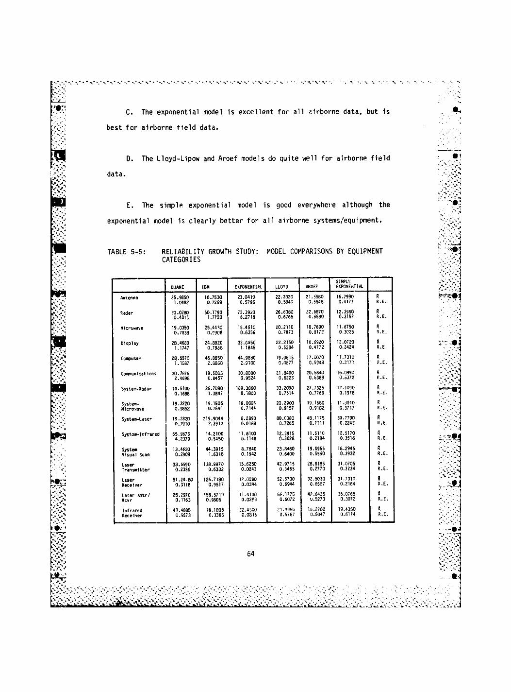
C. The exponential model is excellent for all airborne data, but 1s
best for airborne field data.
D. The Lloyd-Lipow and Aroef models do quite well for airborne field
data.
E. The simple exponential model is good everywhere although the
exponential model is clearly better for all airborne systems/equipment.
TABLE 5-5: RELIABILITY GROWTH STUDY: MODEL COMPARISONS BY EQUIPMENT CATEGORIES
DUANE IBM EXPONENTIAL LLOYD AROEF SIMPLt EXPONENTIAL
Antenna 35.9850 1 .0482
16.7530 0.7259
23.0410 0.5796
22.3320 0.5841
21.5580 0.5548
16.2990 0.4177
R R.E.
Radar 20.0280 0.4015
50.1790 1.7720
72.3920 6.2718
26.6380 0.6765
22.6870 0.6580
12.3560 0.3157
R R.E.
Microwave 19.0350 0.7838
25.4410 0.?908
15.4510 0.6356
20.2110 0.7973
18.7690 0.8172
11.6750 0.3025
R R.E.
Display 28.4680 1.1747
24.8820 0.7958
33.G450 1.1845
22.2150 0.5284
18.6920 0.4772
12.0720 0.2424
R R.E.
Computer 28.5570 irrti 1 . IJO/
46.8850 c« oouO
44.9850 1 m nn L<JIUU
19.0615 r\ (\cn * WW/ /
17.0070 0.5948
11.7310 0.3171
R P..E.
Conmun1cat1ons 30.7875 2.4698
19.5005 0.8457
30.8080 0.9524
21.8400 0.6223
20.5840 0.6389
16.0990 0.o372
ft R.E.
System-Radar 14.5100 0.1688
26.7090 1.3847
189.3860 8.1803
33.2090 0.7514
27.7325 0.7769
12.1090 0.1978
R R.E.
System-Microwave
19.3220 0.9852
19.1505 0,7591
16.0805 0.7144
20.2900 0.9157
19.1680 0.9182
11.J010 0.3717
P. R.E.
System-Laser 19.3820 0.7010
219.9044 2.3913
8.2890 0.0189
80.0380 0.7265
48.1175 0.7111
30.7790 0.2242
R R.E.
System-Infrared 65.9675 4.2379
14.2100 0.5450
11.6100 0.1148
12.3915 0.3028
11.5110 0.2184
12.5170 0.3516
R R.E.
System Visual Scan
13.4620 0.2909
44.3915 1.6316
8.7840 0.1942
23.8460 0.6400
19.6965 0.5550
18.2945 0.3932
R R.E.
Laser Transmitter
33.6590 0.2355
138.9970 0.6332
15.6250 0.0243
42.9715 0.3465
28.8185 0.2770
31.0705 0.3234
R R.E.
Laser Receiver
51.24.80 0.3118
126.7180 0.9517
12.0260 0.0394
52.5700 0.6944
32.5030 0.6537
31.7310 0.2164
R R.E.
Laser Xntr/ Rcvr
25.2970 0.1163
158.571.1 0.9805
11.4100 0.0293
66.1775 0.6072
42.6435 U.5273
36.0765 0.3072
R R.E.
Infrared Receiver
41.4885 0.S573
16.1805 0.3365
22.4500 0.0816
21.^965 0.5767
16.2760 0.5047
19.4350 0.6174
R R.E.
64

The following conclusions can be drawn from Table 5-5:
A. For antennas, all the models except the Duane Model are quite
good.
B. For radar ani microwave systems/equipment, the Duane Model and
the simple exponential model are very good.
C. For display, computer and communications equipment, the Lloyd-
Lipow, Aerof 2nd simple exponential models are good.
D. For infrared systems equipment, all models but the Duane are
excel lent.
E. For all laser systems/equipment, the exponential is vastly super-
ior to all other models.
F. For the visual scan equipment, the exponential model is again
superior to the remaining models.
G. The Duane model, while rarely fitting "best" was seen to fit in
almost all the cases.
5.2.5 Nonrelevant Failures: Reference 56 presents a technique for
determining the learning equation, and thereby, for predicting nonrelevant
failure occurrences. The decrease of nonrelevant failure occurrences over
an equipment's life, especially those due to infant mortality, is a result
65

of a learning process and can be mathematically predicted. This relation-
ship has been demonstrated through use of data obtained from systems com-
posed of many different electronic equipments.
6.0 Reliability Growth Management Techniques: Reliability growth pro-
grams for sophisticated complex systems require considerable resources
si ch as time, money and manpower to achieve the level of system reliability
acceptable to the user. During the growth process, the total system or
major subsystems are tested to failure, system failure modes are deter-
mined and design and/or process changes are implemented to eliminate these
modes or, at least, to decrease their rate of occurrence. If this process
is continued and design and process modifications are made in a competent
manner, then the system reliability will increase.
It is advantageous for the program manager to plan and track this increase
in system reliability during the development program. He may then deter-
mine as early as possible whether or not the system reliability is growing
at a sufficient rate to meet the required goal and allocate available
resources accordingly. In this regard, a program manager needs to deter-
mine from test data the current reliability status of the system, estimate
the rate of growth, and obtain projections of future expected reliability.
Some of the important questions that need to be addressed in planning a
reliability growth program aie:
A. Is a growth test appropriate for this program?
66

B. Is the final reliability objective similar to reliability
achievements made on past programs?
C. What is the expected starting reliability level for the reliabi-
lity growth curve (e.g., 10% of the prediction) and how many hours must the
equipment be preconditioned bafore this starting point is realized?
D. How much time needs to be allotted for growth testing?
E. How many units should be allocated to reliability testing as part
of the overall test program?
F. What minimum test time should be required on each unit on test?
G. What milestones for reliability growth achievement need to be
established?
It must he stressed that the answers to the above questions are not "cook-
book" and each program has to be carefully tailored to the particular
situation and the particular system.
The basic tools for planning a reliability growth program, and thus provid-
ing guidelines to anrwer the aforementioned questions, are discussed in
the following sections.
6.1 Reliability Growth Test or Not; The costs of implementing reliabi-
lity growth into a contract may seem excessive, expecially when one argues
67

that a cont -actor may perform an Informal growth program anyway to discover
gross design errors. However, in past programs discovery of noncompliance
(reject decision in the reliability qualification test) has occurred many
times after full scale engineering development. Because the costs of
design changes are more expensive the later they are implemented, the
customer has only four options after this discovery, none of which is
appetizing:
A. Accept the deficient hardware, which means added life cycle costs
because of additional maintenance, repair and logistics actions along with
lower operational availability.
B. Require correction of defects, which means accepting added delays
and costs.
C. Contract to another supplier for an equivalent equipment, which
undoubtedly involves delays and costs at least, as great as option (B) =
D. Cancel the entire program.
The limited customer options, together with the historical record that
shows an overwhelming preference for option (A) indicates that the threat
of failing a demonstration test if design problems exist may be no threat
at all. This is one reason that the costs of a reliability growth program
are justified. The customer is not only buying a more reliable product,
but is buying visibility to guarantee that the actual status of reliability
68

is known throughout the engineering development phase. With this visibi-
lity, a program manager can assess the program's reliability status and
take a good hard look at why the reliability milestones are not being met.
By doing so, he is in a position to redirect resources in the early phases
of development to avoid having to settle for one of the four options listed
above.
The most cost effective way to grow reliability in a large complex system
is to first identify low reliability equipment via a prediction and then
place extra emphasis on the growth programs of the iow reliability equip-
ment. Fixed length tests have been found to be most appropriate for
reliability growth in terms of cost-effectiveness, since suppliers faced
with testing of uncertain duration tend to protect themselves against
worst case test durations ir. their pricing. Cox and Keely (Ref. 11) have
noted that in many successful reliability programs using reliability
growth philosoph/, approximately 40 to 50% of the total reliability dollar
was allocated for growth testing.
The program manager has two options for a fixed amount of reliability test
time. The op! ons are:
1. A higher reliability level through more growth testing at a cost of
less time for demonstration , and thus a lower confidence in demonstrated
reliability.
2. A higher confidence through demonstration testing at a cost, of less
time for growth testing, and thus lower achieved reliability.
69

These options are shown graphically in Figure 6.1.
FIGURE 6.1: OPTIONS AVAILABLE TO A PROGRAM MANAGER FOR A FIXED RELIABILTY TEST TIME
Once the extent of testing has been determined through a review of the
reliability specified and its relationship to the state-of-the-art, then
evaluations and tradeoffs should be made to determine what tests to include
and/or emphasize.
The nature of the procurement (i.e., new development, production, off-the-
shelf, etc.) will dictate to a large extent the type of tests. If hardware
to be procured is an off-the-shelf commercial product, RDGT may not be
appropriate since the equipment is probably mature and any design change
70

would be difficult to obtain. However, if the off-the-shelf equipment
requires complex rfaces then RDGT becomes more feasible. Figure 6.2
provides soim- c; ance as to the type of test required as a function of
contract ty;a (Ref 23). c
or example, for a new development contract
reliability growth testing is applicable for R&M level A and 8 but not
level C (see Table 6-9 for application levels).
FIGURE 6.2: RELIABILITY TESTS AS A FUNCTION OF CONTRACT TYPE
^ ^ S . COKIRACI
HPE
?LS[ snor
DEVELOPMENT WOOL'CILOH
UCVELUCEN m LOW oa J n J1LU-T0
\ii«r
ufr
7«
SHELF
^ ^ S . COKIRACI
HPE
?LS[ snor
KEU KOOIFLEO HIU HMIFIFP
J1LU-T0
\ii«r
ufr
7«
SHELF
^ ^ S . COKIRACI
HPE
?LS[ snor
R M LEV EL R LEVEL R M LEVEL RW i.k*-: FILX LLVfL (R.ONKLRCfAL)
^ ^ S . COKIRACI
HPE
?LS[ snor A 8 f. A 6 C A 8 c A 8 L A e c
it sr 1'IAN t • 1 • 1 • » • e • 1 • I i • t
R OKOUIIL • < J • ^
I •
R MNOKSTRATION (ACHILKEHENT) » » ( • 1 • • N MHOKSIRAIIIH • « • • * •
J LOT 1 0 II-FUOIITIRR 1
• •
i • • * 1 t t e | £ 1001 •
A - h l G H L S I U U I A B I i n r E F F 0 8 I
C . LOWEST R E L I A U l L I T r EFFOUt ( S tE TABLE 6 - 9 )
Reference 21 presents the following guidelines on when a Reliability
Demonstration lest or Reliability Qualification Test (RQT) is most cost
effective. A demonstration test should be specified only if:
A. Demonstration can be completed sufficiently early for a major
redesign cycle and timely incorporation into production hardware.
71

B. Realistic incentives and penalties are defined and implemented
for reliability achievement or failure.
C. The customer is prepared to take drastic action, up to contract
cancellation, to enforce reliability and schedule guarantees.
Obviously, when included in the program plan, RQT should be employed selec-
tively, applied only to those specific procurement items that satisfy
these criteria.
6.2 Planning for Reliability Growth: Initially, one wishes to depict the
generalized growth pattern for a particular class of systems aeveloped
utilizing historical data on similar systems and equipments and develop-
ment programs in order to make estimates of test time and resources needed.
The data includes expected growth rates and expected initial levels of
reliability. System characteristics that affect growth patterns include
challenge to the state-of-the-art, system complexity, the nature of the
system (ground or airborne, mechanical or electrical, etc.) along with
charecteristics of the development program. Other characteristics that
affect growth patterns are test facilities, failure analysis capabilities
and management's attitude toward a growth program. Thus, the growth rate
is not only a function of the type of equipment being built, but is also
dependent, to some extent, upon the company performing the work. Two
different approaches are commonly used in the analysis of historical data
and the development of planned growth curves. The more traditional
approach has been to treat the entire development program as in idealized
(smooth) process. The other approach treats the development program as a
72

phase-by-phase process. figure 6.3 illustrates the s U evolved for
planning a growth program with continuous fixes implemented during the
program. A similar procedure is used for planning a phase-by-phase type
test (Figure 6.4).
FIGURE 6.3: PLANNED RELIABILITY GROWTH (CONTINUOUS)
DEVELOPMENT OF IDEALIZED GROWTH CURVE
I l
SELECTION OF A SPECIFIED IDEALIZED CURVE APPROPRIATE FOR THE PROGRAM
FIGURE 6.4: PLANNED RELIABILITY GROWTH (PHASE-BY-PHASE)
ANALYSIS OF PREVIOUS PROGRAMS
PHASE D
PHASE C PHASE B
DETERMINATION OF PATTERN AND PHASE CHARACTERISTICS THAT INFLUBKE CURVES.
DEVElOr.ViENT OF PLANNED GROWTH CURVE
PHASE-BY- PHASE CONSTRUCTION
73

In analyzing historical data for planning purposes, care should be exer-
cised to assure that the parameter values are those for the system config-
uration that was being tested and not theoretical values for some hypothet-
ical "paper" configuration.
When the "delayed method" (of implementing fixes) is used, the growth rate
a will be much smaller than it would be using the continuous method. This
is because most of the growth occurs between test phases rather than during
them. One problem with this approach is that neither the Duane, the AMSAA,
nor any other model predicts the magnitude of the jump in reliability from
one phase to another. However, with the continuous method, the test has to
be stopped for every failure and the cost of tying up test resources while
waiting for failure analysis and design changes is prohibitive, making the
delayed method more practical. One should plan what method (delayed fixes
or continuous implementation of fixes) will be used. A mixture of methods
can also be used, for example, if a corrective action is obvious and can be
taken in a timely manner, then the test can be stopped and the fix imple-
mented; however, if no obvious corrective action can be found, then for
practical reasons, an in-depth failure analysis must begin and the fix
implemented at the end of a test phase or as soon as a corrective action
becomes available. In many cases, where the delayed method is used, an
additional equipment is made available to go on test when a failure occurs.
If the planned test time will take too much calendar time, then more than
one equipment must he put on test. If this is the case, then one must take
into account how many equipments will fit into one chamber and how m^ny
chambers must be available for the test in addition to how many work shifts
74
a test must run in order to keep a program on schedule. Reference 38
described an overall test efficiency (defined as a ratio of weekly accumu-
lated relevant test hours to possible relevant test hours) an<' found it to
be approximately 50 percent. Contributing to the inefficiency of testing
are delays associated with definition of corrective actions, lack of test
articles to replace equipment in troubleshooting and repair, and downtime
for repair of test equipment.
In some cases, jumps in reliability associated with delayed fixes are
negative (dips) as shown in Figure 6.5. This situation often occurs at
such times as the beginning of low rate production when the manufacturing
process is in the early stages of a "production learning curve." A new
production reliability growth process must then take place to regain pre-
production reliability. "Dips" may also be caused by new problems that
crop up with a design change to fix some other problem or by equipment
interface problems if the initial testing is not performed on the complete
system configuration.
75

6.2.1 Initial Reliability: The starting point represents an initial
value of reliability for the newly developed hardware and usually falls
within the range of 10 to 40 percent of the inherent or predicted reliabi-
lity after some preconditioning period. Estimates of the starting point
can be derived from prior experiences or based on percentages of the
estimated inherent reliability. Historical data should be used whenever
possible; however, if no prior data is available from a similar system then
a commonly used estimate of 10 to 20 percent of the predicted reliability
can be used. Starting points must take into account the amount of reliabi-
lity control exercised during the design program and the relationship of
the system under development to the state-of-tne-art. Higher starting
points minimize test time. It should be noted that the starting point
reliability applies to the system after preconditioning that allows the
data to "settle down." This means that the preconditioning period is
unplotted, but since the basic plot is cumulative MTBF, the data accumu-
lated during this initial period do influence later results.
Other types of development programs, particularly those for mechanical
systems, may not have as extensive an historical data base to draw upon.
In those cases, starting points can be based on advanced development proto-
type test data or on synthesis of component and subsystem results.
•Vii
6.2.2 The Growth Rate (a)
The growth rate, which is the slope of the growth curve, is governed by the
amount of control, rigor and efficiency by which failures are discovered,
analyzed and corrected through design and quality actions. A large value
of a (a>0.5) reflects a hard-hitting, aggressive reliability program with
77

management support spanning all functions < " a knowledgeable organization,
while a low value of a (a<C.l) reflects the growth in reliability that is
due largely to the need to resolve obvious problems that impact production,
and to implement corrective action resulting from user experience and
complaints. Green (Ref 3) noted that a high growth rate (a) does not
necessarily indicate a good design as is often thought, but it does show a
very thorough effort by the whole organization and particularly by the
reliability engineers, to discover the cause of the failures and eliminate
them. In fact> with excellent design and manufacture a could approach
zero. Negative growth can sometimes be observed when engineering changes
are implemented to improve "performance," at the risk of loss in reliabi-
lity. The maximum value of a that can be expected is not greater than 0.7
because of the lag time associated with revealing failures, analyzing
them, and implementing corrective actions. In many growth programs a
ranges from .3" to .5 as shown in Tables 6-1, 6-2, and 6-3 (Ref 34) which
show the variation of growth rates from in-service use improvement pro-
grams, development tests, and reliability improvement warranties. Table
6-4 summarizes the data showing that the effectiveness of a growth effort
as a function of time, with the development phase growth effort the most
beneficial.
Herd (Ref 34) found that the mean growth rate for a large electronic system
with a single program manager that placed considerable emphasis on devel-
opment testing and had different subcontractors for the component systems
was 0.41, with a standard deviation of 0.20.

Codier (Ref 1) presented some general observations pertaining to growth
rate values. They are that the growth rate (a) is higher:
A. For analog hardware than for digital hardware.
B. For equipment of low maturity than in production hardware.
C. In equipment exposed to severe test conditions than in equipment
undergoing bench tests.
D. In proportion to the hardware oriented reliability improvement
effort.
The differences in growth parameters observed in the various programs
reflect the amount and timeliness of critical engineering information
available for corrective action determination and the nature of the system
(Mechanical, Electronic, etc.).
The Analytical Sciences Corporation (TASC), under contract to RADC, is
developing methodology for predicting reliability growth characteristics
as a function of equipment attributes and program characteristics. The
results will be available as a decision and planning tool around April
1985.
79

TABLE 6-1: RELIABILITY GROWTH RATES FOR ELECTRONIC EQUIPMENT FROM IMPROVEMENT PROGRAMS DURING SERVICE USE
EQUIPMENT OBSERVED a-VALUE
Airborne Teletypewriter -0.10
Airborne Radar Altimeter -0.08
Airborne Search Radar +0.01
Airborne Computer Recorder +0.11
Airborne HF Comnunicat ions +0.12
Airborne UHF Communications +0.13
Airborne Navigation Set +0.14
Shipborne Acquisition Radar +0.14
Shipborne Data Processor +0.17
Airborne Radio Navigation +0.19
Airborne Sonobuoy Receiver +0.19
Airborne Tactical Data Display (A) +0.19
Airborne Radar Scan Converter +0.23
Airborne Tactical Data Display (B) +0.24
Airborne Inertial Navigation +0.30
80

TABLE 6-2: RELIABILITY GROWTH RATES OBSERVED FOR DIFFERENT HAkDWARE SYSTEMS IN DEVELOPMENT TESTS
ITEM OBSERVED a-VALUE
Gatlina Type AA Gun +0.40
Hydro-Mechanical Devices +0.49
Pulse Transmitter, Radav +0.35
Continuous Wave Transmitter +0.35
Aircraft Generators +0.39
Analog Receivers +0.49
Airborne Radar +0.48
Airborne Radar (UK) +0.43
Digital Computer +0.48
Jet Engines +0.35
High-Power Equipment (Power Supply, Microwave Amps)
+0.30
Satellite Comm. Terminal +0.34
Modem (Digital Comm. Terminal) +0.29

TABLE 6-3: EXAMPLES OF RELIABILITY GROWTH RATES UNDER RIW PROGRAMS
ITEM PLANNED a-VALUE
ACTUAL a-VALUE
Gyro +0.13 +0.11
Hydraulic Pump +0.22 +0.29
Airborne Navigation +0.15 ••
TACAN +0.17 -
L , , - ....
TABLE 6-4: COMPARISON OF RELIABILITY GROWTH RATES
TYPE OF PROGRAM
TYPICAL GROWTH RATE PARAMETER (ct)
OPER. TIME TO DOUBLE MTBF (T1 MULTIPLES)
Development Testing +0.11 E A
\J • ~T
RIW In-3vc Operation +0.18 47.0
In-Service Improvement Prog. +0.15 101.6
In-Service Experience +0.05 1,047,587.0

6.3 Reliability Growth Test Time: The test time required to grow the
reliab ility to the specified level 15 an important consideration for
determining costs, manpower and other resources and 1s extremely dependent
upon the growth rate i.nd initial reliability level.
In order to expose latent defects as quickly as possible, efforts can be
made to operate equipment in on/off cycles while applying an environment
including temperature and vibration cycling. High temperature will accel-
erate chemical deterioration, while extreme temperature cycling will pro-
duce thermal stresses and expose mechanical weaknesses, as will vibration.
Repeated on-off switching will produce both transient thermal stresses and
electrical stresses.
Various references recotmiend test times tc be used for growth testing.
There appears to be conflict with regard to these times as shown in Table
6-5. This conflict may be attributed to differences in the magnitude of
the reliability numerical requirements.

TABLE 6-5: VARIATIONS OF RECOMMENDED TEST TIMES PRESENTED IN THE LITERATURE
Recomnended Test Time Reference
1. 20-50 multiples of the required MTBF when the required MTBF is not greater than a few hundred hours (tested in severe environment)
3
2. Not less than a few multiples of the specified MTBF
21
3. 5 to 25 multiples of the required MTBF 37
4. 50 to 100 multiples of the required MTBF 34
1
5. 10 to 25 multiples of the required MTBF 72
6.3.1 Reliability Growth Test Time Estimation for a System: By solving
equation 5.5 for time we have a convenient equation for estimating the test
time needed to "yrow" a system from some initial MTBF to the required
(instantaneous) MTBF.
1
T = [ ( M T B F I N S r ) (K) (1 -ajj a
( E q u . 6 . 1 )
To calculate the test time needed, one must first calculate the constant K.
This is done by using equation 5.2 and substituting an expected growth rate
and an expected initial MTBF c u m after sone initial preconditioning period
Tp^ and then solving for K. Experif with previous reliability growth
programs should provide a m^ans of estimating the initial MTBF point.
However, if experience data is nrt available, as a last resort, the follow-
ing general approximations c~»n be used for planning purposes.

MTBF cum initial
at T D r = .1 X (MTBF predicted) <
E<*
U-
6'
2 )
and T p c - , ( M T B F p r e d . c t e d ) (Equ 6.3)
This provides an estimate of the initial reliability and the length of time
needed to stabilize the data to the point where meaningful assessments and
projections can be made. The lower and upper limits on Tp^ per equipment
should be in the range of 50 hours and 300 hours respectively. Smaller
equipments usually have higher MTBF's and thus the initial condition times
calculated from equation 6.3 may seem excessive. However, Tp c is the total
conditioning period for all equipments to bo put on test, and when it is
divided among the equipments that are going to be tested, the initial
conditioning time per equipment should fall in the range given above. It
is important to understand that there is more than one way to reach the
same goal MTBF for a given amount of test time. This is shown in Figure
6.6. Curve 1 depicts an equipment with a lower initial starting reliabi-
1 i Ly ariu a higher- yrowtri rate that takes T hours to reach its goal MTCP,
Curve 2 represents the same equipment with a higher initial reliability and
a smaller growth rate except with increased emphasis placed on other relia-
bility tasks such as: derating, higher quality parts, and better thermal
management, etc.
85

'#2
i i
L-V
- w vS
t. -*.
V-«
m k' •
$
$ i*
FIGURE 6.6: DIFFERENT WAYS OF REACHING THE SAME MTBF GOAL
-=«# G O A L
u. CO
TIME
6.3.2 Allocating Reliability Growth Test Time to Subsystems: Reference
21 presents a method of allocating reliability growth test time to the most
critical subsystems in order to concentrate the test effort on the region
of maximum potential benefit. This method serves as a check to assure that
test time is not wasted on high MTBF subsystems. An example best illus-
trates this method.
Suppose a system was comprised of the five subsystems shown in Table 6-6
and 5000 hours are available for reliability growth testing.
86
.N " .V.N
bil . »r
' - - - ]
••. V
• ft - » «
•V" K* • «
r . V . W V J a — v ] temem * ^ - ft r ;
• - • ^ . «
Ihr-rV'**!
- . • > *,- v vv.v..,.
V
(V-xMi91
• -•• .N
. -N".
& S 1
V V ', ''I-''
' . 1*. W . . u i : • i -i - - -N -N . ' . A A V ; > J

r.Tr. ^ *VV*-.. - 1 v;v\<n
i y '
TABLE 6-6: SUBSYSTEMS AND THEIR REQUIRED MTBF'S
Subsystem Required MTBF
A 100
B 50
C 750
D 300
E 150
The procedure used to allocate the 5000 hours is to rank the subsystems in
order from the lowest M T B F r e q u i r e d to the highest MTBF r e q i.. f e d and then
divide the total test time available evenly among each subsystem and calcu-
late the number of test multiples of the required MTBF as shown in Table 6-
7.
i. •• m - « * -o > » s >< » >
...
"• .N * :
TABLE 6-7: TEST TIME IN TERMS OF MULTIPLES OF THE REQUIRED MTBF
m
•
Subsystem M T B Frequired Test Multiples of
M T B FRequire;'
B 50 1000/50 = 20
A 100 1000/100 = 10
E 150 1000/150 = 6.7
D 300 1000/300 « 3.3
C 750 1000/750 = 1.3
87
• • Y - W /1
ir.
V" •PA
"M N . ' ' v
v . / - . " 1

Testing for small multiples of the required MTBF 1s not generally as
beneficial, thus subsystems D and C probably should not undergo reliabi-
lity growth testing. The next step would be to go back and reallocate the
test time given to subsystems D and C in order to obtain greater test
multiples of M T B ;
" r eq L,i r e {j (f o r e a c h
subsystem) are in the range of the
recommended test times given in Table 5-5. Another point to b, noted is that
excessive test time on a subsystem may also be inefficient; therefore, a
reallocation may be warranted should the multiples of the M T S Fr e q u - j r e c |
b e
too high.
6.3.3 Test Time Example: Suppose the early part of a reliability growth
test generated failure data as shown in Table 6-8 and one wanted to make an
estimate of the test time needed to achieve an MTBF of 70 hours using this
failure data.
TABLE 6-8: INITIAL GROWTH TEST DATA
Cumulative Test Hours Cumulative MTBF (Hrs)
200 20
525 30
980 35
1500 39
1/00 39
88

Plotted on log-log paper (Figure 6.7) this data shows that reliability 1s
improving in a linear manner.
After a linear relationship becomes apparent, a straight line can be drawn
through the data points and the parameters of the Duane model can be calcu-
lated as follows:
The growth rate: a =
„ - log 35 - log 20 a " log 980 - log 200
a = .35
The practice of using only two data points to calculate a should be
avoided. However, it is done in this example because the two points used
lie on the "eyeballed" line in Figure 6.7 and because equations 5-7 and 5-8
are too lengthy for this simple example.
89

r'-'-v ,• J / . J a r / y ' V / T ^ ^ v T J
Ps-WV-^-''. "f r J s s s s si
.*'». J, I
V •
v..
k'. kv;
» I •
ifc » » '
• i • ,'• >
r .• u • r •S I:'-:
r »
1'V .•
r » • w*
J x ? • > •
'.-•v. i r i *
f t ' ' * -t v v / A
FIGURE 6.7: PLOTTED DATA FOR TEST TIME CALCULATION
TIME f — TJHE R E Q ' D » 2 4 0 0 H o u r s
« » g 7 i 9 1 0 , 0 0 0 f , , , ,
o
! 11!IP!:! UHJ
. ' ^
\ I : • ,• .• / • * I . • •• •• , » • • • ; rf I ' - .
'mv. . y . w . w v : , .'•••;>'•. •

K >
As an alternative method, the slope may be calculated by measuring AMTBF
and AT from the plot with a ruler.
The constant K is calculated using Equation 5.? as follows:
MTBF - I TA
cum K
at T = 200 hours, MTBF c u m = 20, substituting we have:
2 0 = £ ( 2 0 0 ) "3 5
K = .32
£ = 3.13
l l Q i n n a n n t h r * r » a l t o r n a t t w o i t u a t h n H / c o o P i ' n n v o fi 7 \ + r n m i i l a f l 'wo M T R C 1 n n • " 3 >». . -w v< 1 W • V W I I I V I V I I S< I I I W M I I V N I y I I I W W • » / W| I V V U I I I U I U V I » I » k«M I I I I
1
may be extended back to the ordinate and K can be read from the plot at an
abscissa value of 1 hour. It should be noted that if a graphical method is
1 used to find (or K if failure rate versus time is plotted), then the
1
abscissa scale must start at 1. The above method for calculating K is
considered only an approximation as was the case for the previous a calcu-
lation. Better accuracy can be obtained by the use of equations 5-7 and 5-

Thus, tor this example the characteristic growth equation is:
MTBF = 3.13T'3 5
cum
An estimate of the time needed to achieve an Instantaneous 70 hour
MTBF is calculated as follows:
M T B F 4 „ , - M T B F
c u m inst } _ (Equ. 5.6)
70 = M T B F
c u m 1 - .35
M T B Fc u m = 45.4 hours
Substituting this Into the characteristic growth equation for this example
we have:
MTBF = 3.13T'3 5
cum
45.4 = 3.13T'3 5
T = 2095 hours
This compares roughly with the graphical solution of 2400 hours shown 1n
Figure 6.7.
92
Equation 6.1 could have been used as a more direct analytical approach.
T = Q70) (.32) (1-.35JJ 1 A 3 5 = 2095
6.3.4 Planning Test Time: Many reliability growth planners fall into
the trap of determining test time based on the cumulative MTBF reaching the
predicted MTBF. Clarke (Ref 42) showed analytically that there 1s a region
of "no growth" after the current MTBF reaches the predicted MTBF. Failures
precipitated during this period will likely be nonpattern, noncorrectable
ones occurring at a rate of the reciprocal of the predicted (inherent)
MTBF. Therefore, a test structured on the cumulative MTBF reaching the
predicted MTBF would never be completed.
Koo, in a 1981 Westinghouse paper (Ref 51), showed how to manipulate growth
models based on random effect and systematic failures to arrive at test
times required to find a certain percentage of systematic failures, to
reduce the hazard rate to a certain level or to ensure that a certain
number 0 systematic failures occur.
6.4 The Exponential Law for the Appearance of Systematic Failures: Green
(Ref 3) states that through severe environmental test cycles the appear-
ance of systematic failures may follow an exponential law.
The general equation for describing the appearance of systematic failures
is:
93

FTSO "
FTSP n - e "
t / z) (Equ. 6.4)
where: F-J- Q » Types of systematic failure observed
FT S P * TyP
e s systematic failures present
z = Time constant for the environmental test condition
(z decreases with increasing test severity)
t = Cumulative operating time
A time constant of 400 hours has been observed in complex airborne radar
systems. This indicates that on any one equipment, after testing for 1000
hrs under a severe environment, 90% of the systematic defects are revealed
(I.e., 1 - e ( -1 0 0 0
/4 0 0
) = o.9). This is shown graphically 1n Figure 6.8.
FIGURE 6.8: EXPONENTIAL LAW FOR THE APPEARANCE OF SYSTEMATIC FAILURES
&§40
f t w so
* r 2 5
5 0 r- TRIAL A . SEPARATE I R U .i.
B. EA«LY OeVFLG? >v»ENT MOOEl. C uArt. Ot-VcLUrMENT WOOEL
K3 -
F • 3 5 \ l - t ' V S O )
200 4 0 0 6 0 0 BOO KXX) 1200 1 4 0 0 OPERATING HOURS IN SEVERE ENVIRONMENT
I 6 0 0 B O O
94

The optimum test duration per equipment depends on the target MTBF, and
only in the case of an MTBF of several hundred hours or of investigation
into long term wearout failures is it worth extending the test on any one
equipment beyond 1000 to 1500 hours if other equipment are available for
testing.
Green also states that in his experience no single equipment has
accumulated more than 3000 hours of operation per annum following a burn-in
test. 2500 hours is a typical maximum rate por equipment for accumulating
operating hours.
Reference 54 applied the following criteria in order to identify
systematic failures (as opposed to random failures). If either of the
criteria below is met, a possible systematic reliability problem was
identified:
A. The ratio of the number of failed parts to the parts applications
was greater than, or equal to 5 percent, for parts population of greater
than 100.
B. The ratio of the number of failed parts to the parts application
was greater than 20 percent and the number of failures was greater than 1,
for parts population of less than 100.
95

From a mathematical aspect, the exponential law is not compatible with
Duane's model. By differentiating, it is apparent that log of failure rate
will be proportional to time, and not log time as is the case with tho
Duane model. The reason for this is th;«t the Duane model tracks additional
failures such as random failures, quality control type failures, weir-out
failures and repetitive systematic failures where the complete cure has
riot been found.
For a high target MTBF of several hundred or thousands of hours, the
limitations <n development time and money and the inability to use multiple
samples may preclude extensive growth testing and accelerated stress test-
ing may be essential for equipment requirements to be achieved in a cost
effective m.nner. However, accelerated testing must be planned and used
with cautior so unrealistic failure modes will not be revealed.
6.5 Tracking Techniques: The basic reasons to track reliability growth
(or decline) are to make assessments of reliability against the planned
values and to project future .-."liability.
The planned reliability growth provides a standard to which results can be
compared. Assessments can be made without a planned reliability growth
curve; however, the comparisc is subjective because there is no standard
against which to judge and it is a matter of opinion whether or not the
program is progressing satisfactorily. Further, assessment provides a
clear indicator to a program manager when something has gone wrong so he
may know when corrective action needs to be taken.
96

Growth assessment should only be made after some settling down period if a
development phase or test phase change has just taken place or new equip-
ment interfaces have been added. Substantial reliability decline (dips)
may result from infant mortalities resulting from new interfaces and front
the riL'ed for a learning process at the start of a new phase as mentioned
earlier.
Reliability growth projection is used after a trend has been established.
It is particularly useful when the current estimate of reliability varies
significantly from the panned value because it can be used to allot more
or less test time to the current test phase or to intensify the growth
effort tc stimulate a greater growth rate.
Another methud that can be used to track reliability and signa1 trouble in
a growth program is the Triple Tracking method presented by Simkins (Ref
44). This method is a real-time reliability measurement, tracking, and
control approach that is implemented during the development of a new sys-
tem. It allows for multitier growth tracking (equipment, subsystem, and
system) arid provides a high degree of management visability into the effec-
tiveness of corrective actions.
The basic approach is to establish cumulative and instantaneous target
curves using Duane techniques and then plot failures as they occur to
develop actual cumulative o.nd instantaneous curves. The instantaneous
plot is obtained by censoring all correctible failures and not by jumping
up the cumulative plot by a factor of -A-, as is clone with a Duane plot.
97
The cumulative plot is obtained by plotting all relevant failures. Confi-
dence bounds for both the cumulative and instantaneous plots are then
calculated using the chi-squared method. There are three conditions that
must exist for a "red flag" condition which necessitates major redesign,
major change in management control, overhaul or new negotiations on speci-
fication requirements. These out-of-tolerance conditions, all of which
must be present for a "red flag" condition are:
A. Confidence bands about each best estimate of the instantaneous
MTBF do not include the instantaneous targeted curve (planned instan-
taneous MTBF curve).
B. Confidence bands about each best estimate of cumulative MTBF do
not include the cumulative targeted curve (planned cumulative MTBF curve).
C. The projections do not reach the MTBF goal before the end of each
of the three major test periods: development, integration and postinte-
gration.
If only one or two of the above conditions exist then a minor out-of-
tolerance condition, "yellow flag" condition will exist. Minor out-of-
tolerance conditions are those conditions requiring limited actions such
as only one equipment out of a system needing redesign, more frequent
design reviews, special task studies on pattern problems, or more direct
subcontractor control.
98

A benefit of the triple tracking scheme is that, once an out-of-tolerance
condition exists, the program manager knows more about what might be the
cause of it. For example, if the projection and cumulative tracking are
within bourics, but the instantaneous measurements are below target, then
he knows that not enough censoring, at least recent censoring, has taken
place. That is, not enough corrective actions have been found, implemented
aid verified, at least recently.
A;.other useful indicator that can be used in tracking reliabi1ty growth has
beer, observed by Green (Ref 3). He states that if the failures are
classified a? systematic or random, then the ratio of systematic to random
provides a useful indicator of progress. Initially, tne ratio is about
5:1. When the ratio falls to between 1:1 and 2:1, the reliability target
has usually been attained and by that time there is uncertainty i.: the
categorization of failures.
6«5 Confidence Levels: Since the system configurat'ior* is contiriuslly
changing during a reliability growth program, there is usually limited
test data available on the system for a fixed configurst'un. Consequently,
direct estimates of system reliability for a fixed configuration would
generally not enjoy a high degree of confidence and may, therefore, have
little practical value. However, relatively recently confidence intervals
were presented in MIL-HDBK-189 for use with the AMSAA Model.
A unique method for calculating confidence intervals for the Duane model is
presented by Mead (Ref 18). A "least squares" technique is used to fit a
line to Duane growth points. As each successive point contains more

information than its predecessor, the points are progressively weighted in
proportion to the number of failures. A programmable hand calculator
performs this operation rapidly.
With a different program, the same calculator can perform a Monte Carlo
simulation to produce a family of Duane characteristics and to compute the
?rc:n and standard deviation of the log of final MTBF. This enables confi-
dence limits to be obtained for the latter, at less cost than by computer.
Mead states that by obtaining confidence intervals from a growth test a
separate reliability demonstration test may not be necessary. However, it
is believed that this practice should be avoided in order to eliminate any
motivation a contractor might have to hide failures and thus defeat the
purpose of a growth test.
6.7 Cost of a Growth Program: section 6.1 addressed some cost aspects of
» » A 1 1 i l l ! 1 I f >1 n W t l r 4" -1 r \ k r t ^ A n i * T m 1 1 U ^ U n n u n #1 » -s n> I v. I I U U I i i i j y I U N >•< I 3 11 IY o v L/C L U I I S I U C I C U 111 u c u r J 1 r LY WI i c u n c 1 a (JI u y 1 am
is suitable for this test approach. Reference 23 presents additional cost
information pertaining to a reliability program that does and does not
implement reliabilty growth testing.
Six factors play a significant role in reliability improvement and com-
prise the major portion of reliability attributable costs. Table 6-9 shows
these six reliability factors and their various application levsls as
defined for FAA equipment. Level A repre; . ?v i. v h i g h e s t reliabi lity
level; level C the ! owe sr..
100

TABLE 6-9: RELIABILITY ATTRIBUTES AND APPLICATION LEVELS
APPLICATION LEVEL
ATTRIBUTES A B C
PART SELECTION
MICROCIP.CUITS SEMICONDUCTORS RESISTORS CAPACITORS
CLASS A JAN TXV
S T,S
CLASS 8, Bl, B2 JANTX
R R
CLASS C, COMMLRCIAL JAN, COMMERCIAL
P.M P,M,L
DERATING MOST ACCEPTABLE ACCEPTABLE MINIMALLY ACCEPTABLE
ASSEMBLY SCREENING APPLIED NOT APPLIED
VENDOR SURVEILLANCE PERFORMED NOT PERFORMED
R GROWTH TESTING EXTENSIVE MODERATE NONE
R PROGRAM FULL MIL-STD-785 MODIFIED MIL-STD-785 MIL-STD-735 NOT REQ'D
Table 6-10 and Figure 6.9 present the results of an investigation involving
the quantification of the attributes as they are applied to a complex radar
system to determine acquisition cost versus reliability relationships.
101

TABLE 6-10: RELIABILITY ATTRIBUTE LEVELS FOR A GIVEN STATE
RELIABILITY
ATTRIBUTE LEVEL FOR A GIVEN STATE
ATTRIBUTE eo - 9 J
0 3
PART SELECTION C B B A
DERATING C B 8 A
ASSEMBLY SCREENING B B A A
VENDOR SURVEILLANCE R B A A
R GROWTH TESTING C c 8 A
R PROGRAM c • A A
NORMALIZED INCREASE IN ACQUISITION COST
0 2.5X 25X 60*
RELATIVE CHANGE IN MTBF LEVEL (WITH RESPECT TO 9 )
1:1 4:1 18:1 30:1
FIGURE 6.9: PERCENT INCREASE IN ACQUISITION COST - VS - NORMALIZED MTBF
+-> t/>
c o 1-H O
c o 01 </> <0 (V
i- •<-
o </> c •>-t-H 3
cr a* o <
MTBF, 0 (Normalized)
Where: 9Q - represents the MTBF of the equipment when applying the lowest
level associated with each reliability attribute
« /\> v \
A"- V
* i ?»
. • . -»• - >. « V - '-v'V
•r. - W
J- V V \
- o « '
A -- »
- represents the MTBF of the equipment when applying the high-
est level associated with each reliability attribute.

FIGURE 6.10: RELIABILITY TASK COST RELATIONSHIPS
1 0 0 0
Assembly Screening Part
• Selection
/ Derating
^ R Growth Testing
0 5
JL_ L
10 15 20
% Increase In Acquisition Cost
Figure 6.10 shows different reliability task cost relationships on the
data given in Table 6-10 and their payoffs, As can be seen, reliability
growth testing has about, the same magnitude of cost effectiveness as other
well accepted reliability program tasks such as parts selection and
derating.
There is reason to believe this data may be pessimistic with respect to the
cost effectiveness of reliability growth testing because:
A. The data represents only the Federal Aviation Administration's
(FAA) findings and therefore may not be representative of the complexity of
DoD systems. The greater the complexity of the system, the less like'iy it
is that all the problems will be found during the design phase and the more
cost effective growth testing becomes.
103

B. RDGT 1s a cost effective complement to, not substitute for, other
reliability tasks.
C. The systems represented are likely to have greater maturity than
DoD systems. The FAA uses many more off-the-shelf or modified designs.
7.0 Reliability Growth Application Experience: This section will present
an overview of some interesting observations and unique test approaches
that have been found in the course of the st>«dy.
7.1 Current Air Force Applications: A number of Air Force system program
offices (SPO's) were contacted to determine where reliability growth
testing has been applied or is being planned. Table 7-1 lists the program
name, the organization responsible for the program and the type of
system/equipment under development for the information gathered.
•Mk
*
104
* - *• < • •
^ • *. • j . • . - i
V i
iVA'iV* -> -V.TsY. -".Vv .-V --» .

TABLE 7-1: AIR FORCE RELIABILITY GROWTH APPLICATIONS
PROGRAM NAME ORGANIZATION TYPE OF SYSTEM/ EQUIPMENT
HAVE CLEAR (Formerly SEEK TALK)
ESD UHF Radio
SACDIN ESD Conmunications
AFSATCOM ESD Communications
JTIDS ESD Class II Terminal
Simulator SPO ASD Aircraft Simulators
F-16 ASD Aircraft Radar
B1 -B ASD Different Electronic Systems and Some Electro-Mechanical Systems
AMRAAM AD Missile
B-5? Offensive Avionics System (OAS;
ASD Various Onboard Electronic Systems
AWACS ESD Airborne Surveillance Rddd'r, Ddta PruceSsing Displays, Communication, Navigation
AM/ARC-164(V) ASD Communications
A brief overview of the programs listed in Table 7-1 follows:
7.1.1 HAVE CLEAR (Formerly SEEK TALK) - A dedicated reliability growth
test is planned on the airborne equipment at the end of development prior
to a formal RQT. The test length is 2000 hours to grow from an initial MTBF
105
of 55 hours to an MTBF of 250 hours at the start of low rate initial produc-
tion. Reliability growth testing will continue through low rate initial
production with the final jjal being 550 hours.
7.1.2 SACDIN - The initial reliability program included a Failure
Reporting and Corrective Action System (FRACAS) and a reliability demon-
stration test. Past experience showed that little attention was given to
analysis of failures and corrective action. Thus, an integrated growth
test is being conducted both as a development tool and as a determination
of contractual compliance with the required reliability. The Duane model
is being used for planning and tracking purposes.
Thus far, the results of this growth test are showing a growth rate of .3
to .4. Since testing continued before corrective actions were taken and
all failures were counted, some functional areas failed to meet reliabi-
lity milestones.
7.1.3 AFSATCOM - A reliability growth assessment was performed on the
Terminal Segment in a modification of a standard MIL-STD-781 RQT
accept/reject criteria. In order to use the contractually required MIL-
STD-781 B test pi an for a combined growth and demonstration test a ground
rule was made which allowed failures caused by design deficiencies to be
censored from the accept/reject count after the corrective action design
change was implemented and verified. A typical verification test time was
106

used 2 or 3 times the specified MTBF. The procedure used was the topic of a
1977 Reliability and Maintainability Symposium paper "AFSATCOM Terminal
Segment Reliability Test Program" (Ref. 19).
7.1.4 JTIDS - The Class II terminal of the JTIDS System will undergo a
period of reliability growth testing of between 1000 hours and 2000 hours.
The exact lengt, of the growth test is dependent upon whether the current
MTBF equals or exceeds a required MTBF of 500 hours. A formal reliability
demonstration test is required at the completion of growth testing.
7.1.5 Simulator SPO - Because of the small number of aircraft simula-
tors usually procured (10-15), the design changes are implemented during
the program which makes all systems slightly different. This factor, along
with the use of some commercial off-the-shelf equipment, makes for the use
of a reliability growth test as a means to determine contractual compliance
on some programs. The goal MTBK's are usually in the range of 10 to 40
hours and the tests are performed in a laboratory environment since that is
the usual field environment.
7.1.6 F-16 - A dedicated reliability grcwth test was performed on the
first generation Westinghouse radar with good results. A new avionics
package is under development for the F-16 and a growth test is planned for
the new radar. Originally, two equipments were to be tested for 500 hours
each. However, field experience from the first generation radar showed
t'jat most failures occurred soon alter the system was started. Because of
this past experience, it was decided to test 7 radars f r |
r 107 hours each,
for a total test time of about 750 hours. This test length is about 10
107

times the goal MTBF of 70 hours. The growth testing will be part of a full
rellability program.
Field reliability growth on the F-16 fleet is also tracked using a computer
software package. The program can track monthly, quarterly, or cumulative
trends 1n reliability. It also tracks the trends of different work unit
codes to pinpoint developing problem areas. A cumulative growth rate of
about .25 has been observed for the fleet.
7.1.7 Bl-B - A dedicated reliability growth test of 1000 to 2000 hours
is planned. The testing will take place on complex equipment that is
either new or modified. Two first production units of each LRU will be
tested. Each test unit must accumulate a minimum of 25% of the total test
time allotted for the two units. The Duane Model will be used for planning
and tracking purposes and a growth rate of about .3 is expected.
Because of funding and schedule constraints, Environmental Stress Screen-
ing and Reliability Growth Testing are the only reliability tasks required
and contractual compliance with reliability will be determined based on
their results.
7.1.8 AMRAAM - It is planned that six missiles will be put on test to
accumulate 12,500 hours of reliability growth testing. A seventh missile
has been allocated to the test to replace any missile that is undergoing
failure analysis. A conservative 10% of the goal MTBF has been assumed for
the initial starting point. The goal MTBF is 1000 hours. An assumed
108

growth rate of .5 Is being planned and up to 18,000 hours 01' test time may
be used if a lower starting point or growth rate is realized.
All missiles will undergo Environmental Stress Screening and ten missiles
will be allocated for a reliability demonstration test following growth
testing.
7.1.9 B-52 OAS - Initially, reliability requirements were minimal.
When additional funding became available, a dedicated reliability growth
test of 2400 hours per system was chosen. No specific growth rate, start-
ing point or target MTBF were set before the test started.
The test results indicated that 70% of all failures occurred within the
first 1200 hours on most systems. Observations after the test also showed
that the initial MTBF was about 25% of the final MTBF and the growth rate
varied between .3 and .6.
7.1.10 AWACS - The AWACS program used all test data (laboratory, flight
line, flight) to evaluate reliability growth using the Duane concept. The
following types of equipment were tested: data processing, display, iden-
tification, navigation and communication. A brassboard program was imple-
mented which involved a competitive flyoff of two prototype surveillance
radars, each installed in a Boeing 707 aircraft test bed, followed by
evaluation and selection of a winner. Thp competitive nature of the
brassboard phase produced intensive efforts by both competing companies to
quickly identify and eliminate the cause of failure problems. In addition,
reliability growth testing was used as demonstration of contractual
109

requirements. The equipment was accepted if the slope of the current
system MTBF was positive and the current system MTBF was at least the
specified level at any time after the first 500 valid flight hours (about
12 MTBF's). The AWACS reliability growth program was the subject of the
19/5 Reliability and Maintainabil ity Symposium paper entitled "Reliability
Developments - AWACS" (Ref 7).
7.1.11 AN/ARC-164 - The radios accumulated a total of 10,135 valid test
hours with 16 relevant failures occurring during this time. MTBF growth
data was presented weekly throughout the test to provide some indication of
how well the sy? ms were doing. Initial reliability was about 32 percent
of the final reliability after a period of 250 hours per system. A growth
rate between .32 and .35 was realized during the test.
7.2 Program Application Suirmary
From the proceeding program highlights, it can be seen that reliability
growth testing has been and is being applied to a wide variety of systems
under development. Each growth test was tailored (or is being planned) to
meet the specific constraints of the overall development, program.
Scheduling, funding, the number of systems being built and the complexity
of the system seem to be the deciding factors on what type of testing will
take place and whether growth testing will substitute any other reliabi-
lity tasks.
110

8.0 CONCLUSIONS: The impact of equipment and system reliability on oper-
ational readiness and life cycle costs is tremendous. The cost effective
development of reliable equipment for the Air Force is an important respon-
sibility. While the complexity of today's electronic systems makes it
virtually impossible to assure high reliability based on th° results of a
"drawing board" design, some elements of the Air Force have been hesitant
to apply reliability growth techniques.
The reliability achieved on previous military systems has been highly
dependent on the emphasis placed on reliability by program management.
This so-called reliability implementation has been referred to as "ad hoc"
depending on the strength of the program office reliability engineer. Use
of a reliability growth approach gives the status of the reliability pro-
gram more visibility and provides the program manager with a toe' for
planning, tracking and projecting. Current Air Force directives and regu-
lations require that program managers track and manage the reliability
growth process. Earlier revisions assumed that the specified reliability
could be designed into the equipment. Many programs reached an "accept"
MIL-STD-781 decision only after several restarts. Although the unsuccess-
ful attempts weren't called "growth testing," +hat's what they amounted
to. Like a growth test, the equipment reliability improved by design or
manufacturing changes. While reliability growth can and does occur in all
program phases (i.e., development, production, and initial operation), it
is clear that the cost effectiveness of the process becomes greatly dimin-
ished the later the process takes place. By the same token, all potential
problems cannot be surfaced during DT&E, so full growth can't be expected
in development. With the start of each new phase, changes in manufacturing
111

processes and workers introduce a temporary reliability degradation. The
RIW (Reliability Improvement Warranty) is a means of continuing the growth
process into the initial deployment phase.
It should be recognized that reliability growth testing is not a panacea
for developing a reliable product. It is also not a substitute for other
reliability engineering tasks such as parts control and stress derating.
Swett (Ref. 25) several years ago likened reliability development testing
to the linebackers on a football team with the design phase as the defen-
sive line. Both elements are necessary for success whether in football or
reliability design. The key is to "nail the potential reliability problems
as early as possible." A multitude of cases of misunderstanding and
misapplication of the growth testing concept could be cited where after the
fact data has been used to show a growth success story, or as Clarke
stated, there was a "no-growth growth" process. With the complexity of
today's electronic equipment, it is impossible to catch all reliability
problems with the defensive line.
While it is generally agreed that some sort of RDGT is needed as part of
the development process many questions remain regarding implementation of
the concept. Table 8-1 (Previously presented in Section 2.1) lists many of
the questions often expressed by those skeptical of RDGT.
112

TABLE 7-1: AIR FORCE RELIABILITY GROWTH APPLICATIONS
1. Who pays for the RDGT? Does the government.end up paying more?
2. Does RDGT allow contractors to "get away with" a sloppy initial design because they can fix it later at the government's expense?
3. Should reliability growth testing be dedicated or integrated?
4. When should a reliability growth test begin?
5. Should reliability growth be planned for beyond the FSED phase?
6. Should the equipment operate at the fully specified performance level prior to the start of RDGT?
7. Should all development programs have some sort of reliability growth testing?
8. How does the applicability of reliability growth testing v»ry with the following points of a development program?
a. Complexity of equipment and its challenge to the state-of-the-art
b. Operational environment c. Quantity of equipment: to be produced
9. What model(s) should be used?
10. What starting points and growth rates should be used for planning?
11. How much test time will be reqjired?
12. When will corrective actions be implemented and how will failures be counted?
13. Will there: dc u.-; cccept/reject criteria?
14. Should the contractor be responsible for intermediate milestones?
15. Can/should growth testing be incentivized?
16. Does the type of contract affect RDGT decisions?
17. What is a-tequate time for verifying a design fix?
18. What is the relationship between an RQT and RDGT?
19. Who will do the tracking? How and to whom will tiie results/status be reported?
20. How much validity/confidence =houlu be placed on the numerical results of RDGT?
113

Based on the findings of the study, the following paragraphs will address
each of these questions:
1. Who pays for the RDGT? Does the government end up paying more?
The usual case is that the government pays for the RDGT as an additional
reliability program cost and in stretching out the schedule. There have
been situations where contractors have tested on their own prior to an RQT
as their means of reducing the risk of an RQT reject decision. In a
competitive environment, usually the offeror's will riot risk losing the
contract because of the extra cost of nonrequired growth testing. The
point to be made with regard to the RDGT cost is that, regardless of who
pays, the reliability will be improved and the support cost element of the
total life cycle cost equation will be reduced. The savings in support
costs (recurring logistics costs) exceed the additional initial acquisi-
tion cost, resulting in a net savings ir, LCC. The amount of these savings
is dependent on the quantity to be fielded, the maintenance concept, the
sensitivity of LCC to reliability and the level of development required.
It is the old "pay rne now or pay me later situation" which in many cases
makes a program manager's situation difficult because his performance is
mainly based on the "now" performance of cost and schedule. Figure 8.1
showf how ' 3 extra jevelopme"^ cost of an RDGT is "paid back" by reduced
• a c v r l o c o s t e
114
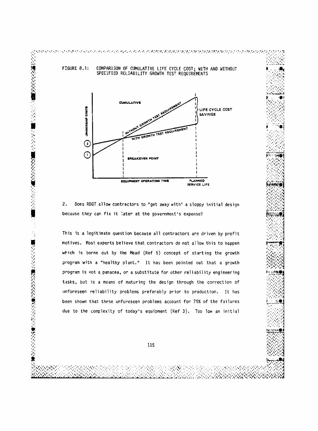
FIGURE 8.1: COMPARISON OF CUMULATIVE LIFE CYCLE COST; WITH AND WITHOUT SPECIFIED RELIABILITY GROWTH TEST REQUIREMENTS
LIFE CYCLE COST SAVINGS
CQUIPMCNT O M R A T 1 N Q TIMS P L A N N E D
S E R V I C E L I F E
2. Does RDGT allow contractors to "get away with" a sloppy initial design
because they can fix it later at the government's expense?
_ -v.
-v •- v
\ ••
This is a legitimate question because all contractors are driven by profit
motives. Most experts believe that contractors do not allow this to happen
which is borne out by the Mead (Ref 5) concept of starting the growth
program with a "healthy plant." It has been pointed out that a growth
program is not a panacea, or a substitute for other reliability engineering
tasks, but is a means of maturing the design through the correction of
unforeseen reliability problems preferably prior to production. It has
been shown that these unforeseen problems account for 75% of the failures
due to the complexity of today's equipment (Ref 3). Too low an initial

reliability (resulting from an inadequate contractor design process) will
necessitate an unrealistic growth rate in order to attain an acceptable
level of reliability in the allocated amount of test time. The growth test
should be considered as an organized search and correction system for
reliability problems that allows problems to be fixed when it is least
expensive. It is oriented towards the efficient determination of correc-
tive action. Solutions are emphasized rather than excuses. It can give a
nontechnical person an appreciation of reliability and a way to measure its
status.
3. Should the RDGT be dedicated or integrated?
The decision regarding whether to allot a specified number of hours for a
dedicated growth test has many pro's and con's. Dedicated tests have the
following advantages:
A. Better control is maintained wit'~ respect to failure occurrence,
documentation and reporting.
B. There is less chance of inducement of failures by operators, test
equipment, etc.
C. The environmental conditions are easier to control.
D. Use of the resulting data for assessment and projection has
greater validity.
116

E. The equipment usually has a pre-established baseline performance
(including meeting environmental qualification) against which to judge
failures.
F. The equipment more closely represents the configuration and manu-
facturing processes to be used in production.
On the other side of the coin are the following arguments for an integrated
RDGT:
A. Since a separate period of testing is not required, the cost is
obviously less.
B. This form of testing is more in line with the cost effective
spirit of RDG1 via earlier detection and correction of failures.
The attributes of dedicated and integrated testing change when an attempt
is made to use the testing as a determination of contractual compliance
with numerical requirements. Reliability problems should be uncovered and
corrected as early as possible to be most cost effective. As pointed out
earlier, an RDGT implies more structured planning, assessment and tracking
than TAAF and FRACAS. As such, a performance baseline needs to be estab-
lished prior to the start c? the RDGT which implies a later start and a
dedicated test. Integrated tests may be more appropriate for small quan-
tity very complex systems and ones with very limited test resources.
117
Waiting for a well controlled dedicated test time with the equipment per-
forming to full specified capacity will in most cases be less cost effec-
tive in providing a vehicle for correction of deficiencies; however, it
offt.'S a better vehicle for assessment and projection. Carrying this to an
extreme, to count on reliability growth later in the equipment life cycle
from the development phase will be very cost ineffective due to the diffi-
culty in incorporating design changes.
When should a reliability growth test begin?
This is partially answered by question number 3 regarding a dedicated vs an
integrated RDGT approach. It should be obvious that the earlier a problem
is found and analyzed, the less costly it is to implement a corrective
n change. Of course, if too early, it is difficult to determine
whe ^r the problem uncovered is a reliability problem or a question of the
design not yet meeting the specified performance criteria. The definition
of rel• bility reflects the ability to perform to some specified criteria
over e. Therefore, tracking of growth can only really be done after the
equipment performs at or near its specified levels. This is not to say
that uncovered reliability problems should not be corrected as early as
possible. It has been said that growth occurs up to two years after IOC
but this includes growth processes involving the human element.
5. Should reliability growth be planned for beyond the FSED phase?
As several authors have mentioned (as referenced in earlier sections),
there are different types of reliability growth in the general sense. Our
118

discussions have been purposely limited to the strict definition of relia-
bility growth to include only reliability improvement as the result of
finding, analyzing and implementing design corrections for reliability
problems uncovered during testing. In this sense, the cost of incorporat-
ing design changes past FSED (Reliability Definition and Dc„-nstration
Phase) may oe prohibitive in terms of ECP's and possible retrofit. The
cost effectiveness of reliability growth varies inversely with the program
phase. Therefore, this type of reliability testing should be used in FSED.
Of course, exceptions to tfrs rule have occurred in the past and will
continue to occur. Cases in point are usually the result of poor field
reliability, where, as the result of an LCC analysis, it becomes cost
effective to undertake some sort of reliability improvement program.
Other situations where thu growth approach may be appropriate are Low Rate
Initial Production (LRIP) programs. While determined to be cost effective
at that point, it would have been much more cost effective to find those
problems and correct them during development. Reliability Improvement
Warranty (RIW) efforts can be thought of as reliability growth in the
production phase. These efforts aren't always effective if a contractor
determines he can make a profit without higher reliability because of
inexpensive maintenance. Other forms of growth as expressed in the pre-
viously mentioned corrments on "no-growth growth" and "endless burn-in"
will occur in production and operational use but are not appropriate for
development.
6. Should the equipment operate at the fully specified performance level
prior to the start of RDGT?
119

•Y>T'
v, % v l v
120
_ t , n..
•-.v."
Waiting until every specified parameter is met is wasting valuable test,
analysis, corrective action and verification time. But on the other hand,
the ability to determine "when is a failure a failure" without a defined
baseline is difficult. If an equipment is performing "almost" to specifi-
cation, determination can be made with respect to most problems as to
whether they are performance related or reliability related. Because this "y
is the case, the time to start is when any meaningful equipment level .•Vol
reliability data can be developed with respect to acceptable measures of
performance. In other words, if a radar is not fully meeting it's specifi- "-V-v-;:
> .'M.
cation with respect to range, that should not prevent test, analysis and
implementation of corrective design on the power supply, signal processor
or other functional elements. Of course, this will result in exposure to
risk because a performance design fix could introduce reliability prob-
lems. If the growth is to be used as an assessment and projection vehicle, S-'v:^
then the configuration should meet all performance requirements. jO,
v.... v
7. Should all development programs have some sort of growth programs?
• v v
The answer to this question is yes in that all programs should analyze and TH
correct failures when they occur in prequalification testing. A distinc-
tion should be in the level of formality of the growth program. The less
challenge there is to the state-of-the-art, the less formal (or rigorous) a
reliability growth program should be. An extreme example would be the case
of procuring off-the-shelf equipment to be part of a military system. In
this situation, which really isn't a development, design flexibility to
correct reliability problems is mainly constrained to newly developed
in'erfaces between the "boxes" making up the system. A rigorous growth
.•'-
%
L '.'ifj
w-r* V v
. i . r_M KM ' » .V.

program would be inappropriate but FRACAS should still be implemented. The
other extreme is a developmental program applying technology that chal-
lenges the state-of-the-art. In this situation a much greater amount of
design ,lexibility to correct unforeseen problems exists. Because the
technology is so new and challenging, it can be expected that a greater
number of unforeseen problems will be surfaced by growth testing. All
programs can benefit from testing to find reliability problems and cor-
recting them prior to deployment, but the number of problems likely to be
corrected and the cost effectiveness of fixing them is greater for designs
which are more complex and challenging to the state-of-the-art.
8. How does the applicability of reliability growth testing *'ary with
the following points of a development program?
A. Complexity of equipment? And challenge to state-of-the-art?
The more complex or challenging the equipment design is, the more likely
there will be unforeseen reliability problems which can be surfaced by a
growth program. However, depending on the operational scenario, the num-
ber of equipments to be deployed and the maintenance concept, there may be
a high LCC payoff in using a reliability growth program to fine tune a
relatively simple design to maximize its reliability. This would apply in
situations where the equipments have extremely high usage rates and LCC
highly sensitive to MTBF.
B. Operational environment?
121

All other factors being equal, the more severe the environment, the higher
the payoff from growth testing. This is because severe environments are
more likely to inflict unforeseen stress associated reliability problems
that need to be corrected.
C. Quantity of equipment to be produced?
The greater the quantities of equipment, the more impact on LCC by reliabi-
lity improvement through a reliability growth effort.
9. What reliability growth model(s) should be used?
The model to be used, as MIL-HDBK-I81 says, is the simplest one that does
the job. Section 5 went into detail on what models apply best for a
variety of situations. Certainly, the Duane is most common, probably with
the AMSAA second. They both have advantages; the Duane being simple with
parameters having an easily recognizable physical interpretation, and the
AMSAA having rigorous statistical procedures associated with it. MIL-STD-
189 suggests the Duane for planning and the AMSAA for assessment and
cracking. When an RQT is required, the RDGT should be planned and tracked
using the Duane model; otherwise, the AMSAA model is recommended for track-
ing because it allows for the calculation of confidence limits around the
data.
10. What starting points and growth rates should be used for planning?
122

For planning an RDGT, growth rates and starting periods should be based on
experience with the development of similar systems. Rules of thumb, such
as a starting point of 1C% of the inherent (predicted) MTBF at a test time
of one half tne inherent MTBF and a growth rate of 0.4 or 0.5, have been
suggested. Growth is not a naturally occurring process but rather takes
place when failure modes/mechanisms are systematically removed. There-
fore, it is always better to use historical data based on the experience of
the particular contractor on similar programs. As a planning tool, RADC
has currently underway (reference Section 6.2.2) a research effort that
will provide guidance regarding the characteristics to be expected on a
particular reliability growth program based on both equipment characteris-
tics and program attributes.
11. How much test time will be required?
The test time required, as shown previously, is a function of the initial
level of reliability as well as the growth rate. Appendix A gives tables
for various final target MTBF's. The literature is rather confusing
regarding growth test time recomendations as shown in Table 6-5. Because
of the rates at which systematic defects are likely to occur and potential
wearout mechanisms, test planning must also address test time on a per-
equipment basis. Test efficiency is a driver in determining how much
calendar time will be required to accumulate the required test hours. All
these factors make a fixed time reliability growth test the best choice for
planning and for costing by a contractor in a competitive situation. Vari-
ous persons have suggested accelerating the test by way of more severe
stress levels as a means of shortening the time; however, extreme caution
123
must, be exercised so that new failure modes aren't introduced that wouldn't
occur in the operational environment. Some authors have described associ-
ating an acceleration factor during growth testing as a "black art."
12. When should corrective actions be implemented?
Ideally the corrective actions should be put in right after the discovery
of the problem so that the growth process is continuous and the verifica-
tion time for each fix is maximized. In this situation plotted data would
be smooth. To carry this out in practice would mean tying up test
resources until a fix is found for every failure, which cannot be done in
real life. The AMSAA (MIL-HDBK-189) approach is to use a phase-by-phase
process where fixes are implemented at the end of each test phase so that
within phases the growth is continuous and between phases there are relia-
bility "jumps." The problem with this approach is that thsre isn't any way
of judging how large (or small) the jumps will be. Several authors advo-
cate plotting only "failure sources," or first time failure occurrences,
during growth tracking. With this approach, further incidents of these
modes, following the first occurrence, are not counted as long as a correc-
tive action is implemented with adequate verification time prior to test
completion. Others keep track of the progress both ways, "culled" data and
all data. The mathematics of models show that the growth process is a self
purging one where the model itself takes care of eliminating earlier
failures.
Will there be an accept/reject criteria?
124

The purpose of reliability growth testing is to u.,cover failures and take
corrective actions to prevent their recurrence. Having an accept/reject
criteria is a negative contractor incentive towards this purpose. Moni-
toring the contractors progress and loosely defined thresholds are needed
but placing accept/reject criteria, or using a growth test as a Hemonstra-
tion, defeat the purpose of running them.
14. Should the contractor be responsible for intermediate milestones?
A degree of progress monitoring is necessary even when the contractor knows
that following the reliability growth test he will be held accountable by a
final RQT. Tight thresholds make the test an RQT in disguise. General
guidance for determining the acceptability of progress is expressed in
MIL-S'D-1635 (reference Section 6.5) and in the IBM triple tracking
method. It must be remembered what the purpose of the test is; there
should be no incentives for contractors to hide failures.
15. Can/should growth testing be incentivized?
Reliability growth can be incentivized but shouldn't be. To reward a
contractor for meeting a certain threshold in a shorter time or by indicat-
ing "if the RDGT results are good, the RQT will be waived," the contrac-
tor's incentive to "find and fix" is diminished. The growth test's primary
purpose is to improve the design, not to evaluate the design.
16. Does the type of contract affect RDGT decisions?
125
The type of development contract is a procurement strategy decision and is
usually determined as a function of program risks. Development contracts
are generally a "cost plus" type which may or may not include incentives.
Production contracts which are much easier to price, because costs can be
defined, are usually some form of "fixed price" ones. It has already been
stated that contracts with incentives based on reliability growth give
contractors a reason to hide failures, which is counterproductive. If
fixed length reliability growth testing is used, it really doesn't matter
what the contract type is because the test can easily be priced, even as a
separately priced contract it-m.
17. What is adequate tirr.: to verify a design fix?
Most persons agree that the verification time to prove that a design fix
has eliminated a particular failure mode depends on what the mode is, what
the fix is and how the fix interacts with the rest of the design. It must
be long enough to assure that, even though the original problem has been
corrected, new time dependent failure modes haven't been introduced by the
fix. A good rule of thumb is that the time should be at '.east one MTBF
(predicted).
18. What is the relationship between an RQT and RDGT?
The RQT is an "accounting task" used to measure the reliability of a fixed
design configuration. It has the benefit of holding the contractor ac-
countable some day down the road from his initial design process. Ar, such,
126

he is encouraged to seriously carry out the other design related reliabi-
lity tasks. The RDGT is an "engineering task" designed to improve the
design reliability. It recognizes that the drawing board design of a
complex system cannot be perfect from a reliability point of view and
allocates the necessary time to fine tune the design by finding problems
and designing them out. Monitoring, tracking and assessing the resulting
data gives insight into the efficiency of the process and provides n o n l i -
ability persons with a tool for evaluating the development's reliability
status and for reallocating resources when necessary. The forms of testing
serve very different purposes and complement each other in development of
systems and equipments. An RDGT is not a substitute for an RQT, or other
reliability design tasks.
19- Who will do the tracking? How and when will the results/status be
reported?
When an RDGT is invoked in conjunction with an RQT, as reconmended, the
close monitoring of contractor results isn't as critical as when enly an
RDGT is being required. If an RQT is providing the accountability at some
later time, the RDGT can be thought of as a means of increasing the chances
of passing the RQT. Of course, as has not been the case in many RQT's in
the past, the procuring activity has to exercise its redesign options
should a reject decision be reached in RQT. Still, wich an RQT hanging
over his head, a contractor may still shortcut his reliability design
approaches hoping to pass the RQT by the usual practices of declaring
failures nonrelevant, induced by test equipment and the like. Therefore,
the growth process should always be monitored by the AF program office,
127

with the degree of scrutiny dependent on how the results are to be used.
Reporting of the results and status is not clearly defined under present
reliability standards and data item descriptions (DID's). No specific
DID's exist for reliability growth. Existing ones written for the RQT must
be tailored for this application.
20. How much validity/condifence should be placed on the numerical
results of RDGT?
Associating a hard reliability estimate from a growth process, while math-
ematically practical, has the tone of an assessment process rather t.ian an
improvement process, esoecially if an RQT assessment will not follow the
RDGT. In an ideal situation, where contractors are not driven by profit
motives, a reliability growth test could serve as an improvement and
assessment vehicle. Since this is not the real world, the best that can be
done if meaningful quantitative results are needed without an RQT, is to
closely monitor the contractor RDGT. Use of the AMSAA model provides the
necessary statistical procedures for associating confidence levels with
reliability results. In doing so, closer control over the operating condi-
tions and failure determinations of the RDGT must be exercised than if the
test is for improvement purposes only. A better approach is to use a less
closely controlled growth test as an improvement technique (or a struc-
tured extension of FRACAS, with greater emphasis on corrective action) to
fine tune the design as insurance of an accept decision in an RQT. With
this approach, monitoring an improvement trend is more appropriate than
development of hard reliability estimates. Then use a closely controlled
RQT to determine acceptance and predict operational results.
128

8.1 Summary of Conclusions: Certainly no one in the development business
can argue against uncovering problems and correcting them. The RDGT has
been proved to be an organized approach to doing just that. It does not
replace other design oriented reliability tasks. It may add to the acqui-
sition cost of a system, but the reduced risk of failing a reliability
demonstration and the reduction in operation and support costs more than
offset this. Most skeptical comments regarding the growth concept have
their origin in situations where growth techniques have been misapplied or
used as a panacea trying to bail out a poor design. When applied properly
and not substituted for an RQT, an RDGT is an extremely cost effective task
in the development process. Unfortunately, many success stories written
around the concept are of the misapplication type which have resulted in
"turning-off" reliability practioners to the concept. The complexity of
today's equipment necessitates recognition of the fact that designs cannot
be perfect off the drawing board. As such, a properly defined and managed
reliability growth program is a must for today's development efforts.
RADC's new R&D study "Reliability Growth Prediction" will serve as an
excellent complement to MIL-HDBK-189 and MIL-STD-1635 in assuring that the
concept is properly applied.
129

«r"_
mi „V
•v f • . - V - . . V
r rv - -.v V3
A P P E N D I X A - . - . » - " • '
• i, . - » • • • * * o »
\
T E S T T I M E T A B L E S
i •
L « - ' • - fc » w
•f'A
142
1 V
V//.-.V-
It-
The following tables contain estimated test times calculated by using V v V % jv
equations 6.1, 6.2, 6.3 and 5.2. These times are the number of hours
needed for the instantaneous Duane plot to reach the MTBF goal (9q). The
predicte I MTBF and the initial conditioning period (assuming Equ. 6.3
holds) are given at the top of each page. The starting MTBF, stated as a
percentage of the predicted MTBF, is varied in increments of 5 percent
across the top of each table. The growth rate (a) is varied along the left . . . . N-VV'•-•<>
side of the table in increments of .05. The blank spaces in the table vy/V;-.^
represent test time results which are less than five times the predicted
MTBF and are therefore not recommended. A minimum test time of 5 times the
predicted MTBF should be used in these cases. " > V \ "VJ i
V V
VY-Y-WVlj
v v
. - - . • . • - v s .
V
* »


m * ' ' ' 1
f f f t k -f S V
tfvVv
Kvv vv •
iV'.'. v .•
- f i t s
j v v v v
s / ss / .'
I 'i V
7am7 > / / / F ^ V ^ ' v v & I L ^ v - V
2> i
TABLE A.2: RELIABILITY GROWTH TEST TIME (9 = 50 HOURS)
PREDICTED MTBF (6 ) = 50 HOURS
INITIAL CONDITIONING PERIOD .5 (9 ) P
a Growth Rate
.20
.25
.30
.35
.40
.45
.50
.55
.60
5%
26,214,400
1,265.625
165,335
33,074
12,470
5,154
2 , ^ 9 9
1,358
799
25 HOURS
Starting Point % of 9
10% 15%
P
20% 25% 30% 35% 40%
819,200
79,101
16,403
5,254
2,204
1,104
624
385
251
107,878 25,600
15,625
4,245
1,649
799
448
277
4,943
1,627
725
389
8,388 3,371 1,559
2,025
773
383
976
421
527
251
800
308
V
W-.VV
i V v v V v V / '
I vV',Vv>'',' % / ^ v y y y y y

t~* «-«
J • f / , s \
V S N - V
» « a «
> I
TABLE A.3: RELIABILITY GROWTH TEST TIME (9p - 75HOURS)
PREDICTED MTBF (9 ) = 75 HOURS
INITIAL CONDITIONING PERIOD .5 (0 )
a Growth Rate
.20
.25
.30
.35
.40
.45
.50
.55
.60
5%
248,003
57,111
18,706
7,731
3,749
2,037
1,199
37.5 HOURS
Starting Point % of 9
10% 15%
P
2 0 % 25% 30% 35% 40%
39,321,600 1,228,800 161,817 38,400 12,582 5,056 2,339 1,200
1,898,437 118,652 23,437 7,415 3,037 1,464
24,605
7,882
3,306
1,656
937
5 77
377
6,368 2,441 1,160 631
790
377
2,474 1,087
1,200
672
575
416
463

f. V V' TABLE A.4: RELIABILITY GROWTH TEST TIME (0p = 100 HOURS)
t r • i f •'
V-.'V-. f v v >
S "i -v.
r V V V
' r"
v-.-v-. * ' / J , ' v. v •*v *,
'.•',• V, 'j '7 I
A '* * , ^ ^
f V / V
KK r/
I'-:-: •• u('. .
S v v v ' / .' r' ,
3=» 1 <T>
PREDICTED MTBF (0 p) = 100 HOURS
INITIAL CONDITIONING PERIOD .5 (0 ) P
a Growth Rate
.20
.25
.30
.35
.40
.45
.50
,55
.60
5%
2,531,250
330,671
76,149
24,941
10,308
4,999
2,716
1,599
50 HOURS
Starting Point % of 9
10% 15%
P
20% 25% 30% 35%
158,203 31,250 9,887 4,050 1,953 1,054
32,806
10,509
4,409
2 , 2 0 S
1,249
770
503
8,491 3,254 1,547
3,299 1,450
1,599
897
555
766
779
842 503
40%
52,428,800 1,638,400 215,756 51,200 16,777 6,742 3,119 1,599
617

Si* x t t & f t ' . ' < < V*. w kv; L V \ S
fc'vVV
£ v v \ V . V "r
I I • V V V
' «
PlrS s •• "v / / « t V v , V ' / v .
' • . *
S r • .'*
i "V V '. f / v . •,
¥ s ; W-. ' J f t c- •>
' / .* /
r, •
' '«•. ' - ' A k X - ' V
r • • '.
1»
TABLE A.5: RELIABILITY GROWTH TEST TIME (0 = 150 HOURS)
PREDICTED MTBF (6 ) = 150 HOURS
INITIAL CONDITIONING PERIGD .5 (9 p) = 75 HOURS
a Growth Rate
.20
.25
.30
. 35
.40
.45
.50
.55
.60
5%
78,643,200
3,796,875
496,007
114,223
37,412
15,462
7,499
4,074
2,399
Starting Point % of 0
10% 15%
P
20%
2,457,600
237,304
49,210
15,764
6,613
3,313
1,874
1,155
755
3?^,634
46,875
12,737
4,949
2,400
1,345
833
76,800
14,831
4,882
2,175
1,169
25% 30% 35%
25,165
6.075
2,320
1,150
10,113
2,929
1,263
4,679
1,581
755
40%
2,400
926
F- • ' » I W v - A - v » •/ • ."J- ;•»;•.'•;-.V.V/.1 5 v v v v / v / v j v ^ v v v • • W f ^ J - ; % - t \ • » • : • 4 I .
v v •, s «
• - . • ,* <'Jft »' *' ''

F- y v
S S W
m 5 » V v V
g w i v w .
& V Y *
r-;
» V k *•
rV v,
I CO
TABLE A.6: RELIABILITY GROWTH TEST TIME (9p = 200 HOURS)
PREDICTED MTBF (9 ) = 200 HOURS P
INITIAL CONDITIONING PERIOD .5 (9 ) = 10C HOURS P
a Growth Rate
.20
.25
.30
.35
.40
.45
.50
.55
.60
S "v Y
% » I
V-. - y - x W W - ? ' ? -•r , / . /
Vrnm-
5%
104,857,599
5,062,500
661,343
152,298
49,883
20,616
9,999
5,432
3,199
Starting Point % of 9
10% 15%
P
20% 25% 30% 35% 40%
3,276,799
316,406
65,613
21s018
8,818
4,418
2,499
1,540
1,007
431,512
62,500
16,983
6,599
3,199
1,794
1,111
102,399
19,775
6,509
2,900
1,558
33,554
8,100
3,094
1,533
13,484
3,906
1,684
6,238
2,108
1,007
3,199
1,235
" > " • " - . ' . . ' . ' /t-7 - , , ' A 19' '<• .''.'fRV .' / -• • n a g s - ; ; ' r ^ W V ' / > V V /_ !!• '. ' •'.Y , .'*'•'•-'.' I* . . . - ,. . <• J

TABLE A.7: RELIABILITY GROWTH TEST TIME (0 = 1000 HOURS)
i io
PREDICTED MTBF (0 ) = 1000 HOURS
INITIAL CONDITIONING PERIOD .5 (0 p)
a Growth Rate
.20
.25
.30
.35
.40
.45
.50
.55
.60
5%
6,328,125
826,678
190,372
62,353
25,770
12,499
6,790
3,999
125 HOURS
Starting Point % of 9
10% 15%
P
20% 25% 30% 35% 40%
131,072,000 4,096,000 539,390 128,000 41,943 16,855 7,798 4,000
395,507
82,016
26,273
11,022
5,522
3,124
1,925
1,259
78,125 24,719 10,125 4,882 2,635 1,544
21,229 8,137 3,867 2,106 1,259
8,249 3,626 1,916
4,000 1,948
2,243
1,388

TABLE A.8: RELIABILITY GROWTH TEST TIME (0 = 1000 HOURS)
PREDICTED MTBF (0 ) = 1000 HOURS
INITIAL CONDITIONING PERIOD .5 (0 p)
a Growth Rate
.20
.25
.30
.35
.40
.45
.50
.55
.60
5%
992,014
228,447
74,824
30,924
14,999
8,148
4,799
150 HOURS
Starting Point % of 9
10% 15%
P
20% 25% 30% 35%
98,420
31,528
13,227
6,627
3,749
2,310
1,511
25,474 9,764 4,641 2,527 1,511
9,898 4,351 2,300
4,795 2,338
2,691
1,666
40%
157,286,400 4,915,200 647,269 153,600 50,331 20,227 9,358 4,799
7,593,750 474,609 93,750 29,663 12,150 5,859 3,162 1,853

TABLE A.9: RELIABILITY GROWTH TEST TIME (0 = 1000 HOURS)
PREDICTED MTBF (0 ) = 1000 HOURS
INITIAL CONDITIONING PERIOD .5 (0 p)
a Growth Rate
.20
.25
.30
.35
.40
.45
.50
.55
.60
5%
8,859,375
266,522
87,295
36,078
17,499
9,506
5,599
175 HOURS
Starting Point % of 0
10% 15%
P
20% 25% 30% 35% 40%
183,500,800 5,734,400 755,147 179,200 58,720 23,598 10,918 5,599
553,710 109,375 34,606 14,175 6,835 3,689 2,162
1,157,350 114,823 29,720 11,391 5,414 2,948 1,763
36,783 11,542 5,076 2,683
15,431
7,731
4,374
2,695
1,763
5,599
3,140
1,944
2,727

r ~ ~ -L---inw r-. . < . jr . < ' . • s s s i t v . f i r T r i T y r > v . ' - i p e ^ g V * ' •, '. . yim ,". , . t1 -'iij, . . i, i, •. • '. '«* V v / / •* F-" '•" •"
1 l
1 r- ,
s
' j *< J
-V vV".
• i J
I I p Y
1 ,
-V.V',
r,vvY"
Y.'V-:
Y Y ; t * . t V . V ,
V /
^ / /
r » J « J t J s i ) i
• *» » 1 f
r » r V /
L*'/'.'
V.•* >•
> I
TABLE A.10: RELIABILITY GROWTH TEST TIME (0 = 400 HOURS)
PREDICTED MTBF (0 )
INITIAL CONDITIONING
a Growth Rate
.20
.25
.30
.35
.40
.45
.50
.55
.60
= 400 HOURS
PERIOD .5 (0 )
5%
10,125,000
1,322,686
304,596
99,766
41,232
19,999
10,864
6,399
200 HOURS
Starting Point % cf 0
10% 15%
P
20% 25% 30% 35% 40%
209,715,200 6,553,600 863,025 204,800 67.108 26,969 12,477 6,399
632,812
131,227
42,037
17,636
8,836
4,999
3,080
2,015
125,000 39,550 16,200 7,812 4,216 2,471
33,966 13,019
13,198 5,801
6,188 3,369 2,015
3,066
6,399
3,588
2,222
3,117
*,. v v v'.! ;
• •
R R
m - i m
tkt- • "<"< •. •• w r
• / - v . - v v , • l \ > v y A
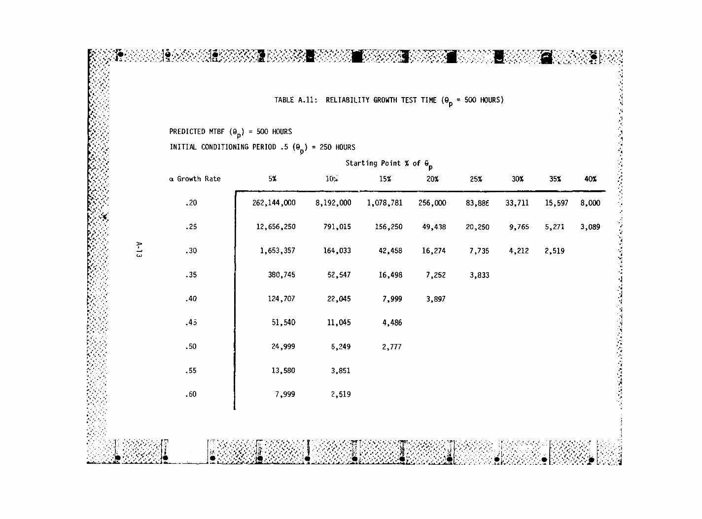
TABLE A.11: RELIABILITY GROWTH TEST TIME (0 = 1000 HOURS)
PREDICTED MTBF (0 ) = 1000 HOURS
INITIAL CONDITIONING PERIOD .5 (0 p)
a Growth Rate
.20
.25
.30
.35
.40
.45
.50
.55
.60
5%
12,656,250
1,653,357
380,745
124,707
51,540
24,999
13,580
7,999
250 HOURS
Starting Point % of G,
ICfc 15%
P
20% 25% 30% 35% 40%
262,144,000 8,192,000 1,078,781 256,000 83,886 33,711 15,597 8,000
791,015 156,250 49,438 20,250 9,765 5,271 3,089
164,033
22,045
11,045
6,249
3,851
2,519
42,458 16,274 7,735 4,212 2,519
52,547 16,498 7,252 3,833
7,999 3,897
4,486
2,777

TABLE A.12: RELIABILITY GROWTH TEST TIME (0 = 1000 HOURS)
i
PREDICTED MTBF (0 ) = 1000 HOURS
INITIAL CONDITIONING PERIOD .5 (0 p)
a Growth Rate
.20
.25
.30
.35
.40
.45
.50
.55
.60
5%
15,187,500
456,895
149,649
61.848
29,999
16,296
9,599
300 HOURS
Starting Point % of 9,
10% 15%
P
20% 25% 30% 35% 40%
314,572,800 9,830,400 1,294,538 307,200 100,663 40,454 18,716 9,600
949,218 187,500 59,326 24,300 11,718 6,325 3,707
1,984,029 196,840
63,056
26,454
13,254
7,499
4,621
3,023
50,949 19,529 9,282 5,054 3,023
19,797 8,702 4,600
9,599 4,676
5,383
3,333

it*.
E S v v tv r> f : Sr*» V,>
m F v V V
Y V ^ . 't
m «* «•
* } 11 r/v-;-; »' ' * »* I . > k W f - V . V . / / .•
h \ ••
s i . < f r f
V ^ V j V V i 'ss.sy.ssi
V V
v.v
V v
> I
TABLE A.13: RELIABILITY GROWTH TEST TIME (0 = 800 HOURS)
PREDICTED MTBF (0 ) = 800 HOURS
INITIAL CONDITIONING PERIOD .5 (9 p)
a Growth Rate
.20
.25
.30
.35
.40
.45
.50
.55
.60
5%
2,645,372
609,193
199,532
82,464
39,999
2 1 , / ^ 9
12,799
400 HOURS
Starting Point % of 9,
10% 15%
P
20% 25% 3or; 35% 40%
419,430,400 13,107,200 1,726,051 409,600 134,217 53,939 24,955 12,800
20,250,000 1,265,625
262,454
84,075
35,272
17,673
9,999
6,161
4,031
250,000 79,101 32,400 15,625 8,433 4,943
67,933 26,038 12,376 6,739 4,031
26,396 11,603
12,799
7,177
4,444
6,235
6,133
• i V i ,4 -3 A
..1
A * 4
-.1 fi
•'4
•'A 4
•a
: • -i > i _ >
..•.',<- i ' - V V v V . . yyyy.-.,\r
> < t . i r J '
1
' ii i j '

TABLE A.14: RELIABILITY GROWTH TEST TIME (0 = 1000 HOURS)
PREDICTED MTBF (0 ) = 1000 HOURS
INITIAL CONDITIONING PERIOD .5 (0 p)
a Growth Rate
.20
.25
.30
• 35
.40
.45
.50
.55
.60
5%
761,491
249,415
103,080
49,999
27,161
15,999
500 HOURS
Starting Point % of 0 p
10% 15% 20% 25% 30% 35% 40%
524,288,001 16,384,000 2,157,563 512,000 167,772 67,423 31,194 16,000
25,312,500 1,582,031
105,094
44.090
22.091
12,499
7,702
5,039
84,916 98,876 40,500 19,531 10,542 6,179
3,306,715 328,067 312,500 32,548 7,666 8,424 5,039
15,999 14,504
8,972 7,794
5,555

i ,
>>
APPi_,'UIX B
B I B L I O G R A P H Y
->Y'
-.1
• i.
B-l
- * "v * " • " • - . I - *

BIBLIOGRAPHY
1. Codier, E.O., Reliability Growth in Real Life, Proceedings 1968
Annual Reliability and Maintainability Symposium.
2. Selby, J.D. and Miller, S.G., Reliability Planning and Management -
RPM, General Electric Company, Aerospace Electronic Systems, Utica,
NY.
3. Green, J.E., The Problems of Reliability Growth and Demonstration
with Military Electronics, Microelectronics and Reliability, Vol 12,
PP. 513-520, 1973.
4. Prasad, P.S.K., Reliability Prediction and Growth Studies - How Accu-
rate and Useful, Microelectronics and Reliability, Vol 13, PP. 195-
202, 1974.
5. Mead, P.H., Reliability Growth Of Electronic Equipment, Microelec-
tronics and Reliability, Vol 1', PP. 439-443, 1975.
6. Bezat, A.; Montague, L., and Norquist, V., Growth Modeling Improves
Reliability Predictions, Proceedings 1975 Annual Reliability and
Maintainability Symposium.
7. Peacore, E.J., Reliability Developments - AWACS, Proceedings 1975
Annual Reliability and Maintainability Symposium.

Cox, T.; Lavery, J. and Meade, C., Reliability Growth Management in
USAMC, Proceedings 1975 Annual Reliability and Maintainability
Symposium.
Crow, L.H., On Tracking Reliability Growth, Proceedings 1975 Annual
Reliability and Maintainability Symposium.
Schafer, R.E.; Sal lee, R.B. and Torrez, J.D., Reliability Growth
Study, Hughes Aircraft Company, RADC-TR-75-253, October, 1975.
Cox, T.D., and Keely, J., Reliability Growth Management of SATCOM
Terminals, Proceedings 1976 Annual Reliability and Maintainability
Symposium.
Jayachandran, T. and Moore, L.R., A Comparison of Reliability Growth
Models, IEEE Transactions on Reliability, Vol R-25, No 1, April 1976.
Bird, G.T. and Herd, G.R., Avionics Reliability Control During Devel-
opment, Advisory Group for Aerospace Research and Development (AGARD)
Lecture Series No 81, 7 Rue Ancelle, 92200 Neui1ly-Sur-Seine, France,
March 1976.
Green, J.E., Reliability Growth Modeling for Avionics, AGARD Lecture
Series No 8"!, 7 Rue Ancelle, 92200 Neuilly-Sur-Seine, France, March
1976.
B-3

Sumerlin, W.T., Illusory Reliability Growth, AGARD Lecture Series No
81, 7 Rue Ancelle, 92200 Neui1ly-Sur-Siene, France, March 1976.
Beacher, D.E. and Chaptman, W.A., Reliability Proving for Commercial
Products, Proceedings 1977 Annual Reliability and Maintainability
Symposium.
Plouff, W.E., Avioriic Reliability Experience: AR-104 and 781B, Pro-
ceedings 1977 Annual Reliability and Maintainability Symposium.
Mead, P.H., Duane Growth Model: Estimation of Final MTBF with Confid-
ence Limits Using a Hand Calculator, Proceedings 1977 Annual Reliabi-
lity and Maintainability Symposium.
Hassett, R.P. and Oonson, E.C., AFSATCOM Terminal Segment Reliability
Test Program, Proceedings 1977 Annual Reliability and Maintainability
Symposium.
Fertig, K.W. and Murthy, V.K., Models for Reliability Growth During
Burn-in: Theory and Applications, Proceedings 197G Annual Reliabi-
lity and Maintainability Symposium.
Murden, W.P. and Hoy, W.W., Defining Cost-Effective System Effective-
ness and Safety Programs, Proceedings 1978 Annual Reliability and
Maintainability Symposium.
B-4
Li 1
ius, W.A., Reliabi1ity Growth Planning and Control, Proceedings
1978 Reliability and Maintainability Symposium.
Lakner, A.A.; Anderson, R.T. and DiGianfilippo, A., Cost Effective
Reliability Testing, Proceedings 1978 Reliability and Maintainability
Symposium.
Clarke, J.M., and Cougan, W.P., RPM - A Recent Real Life Case History,
Proceedings 1978 Annual Reliability and Maintainability Symposium.
Swett, B.H., Reliability Growth Management, Proceedings - Institute
of Environmental Sciences, 1978.
Evans, J.C. and Legreid, S.I., Reliability Growth on B-52 FLIR Sys-
tem, Proceedings - Institute of Environmental Sciences, 1978.
Bennett, R.W. and Oglssby, R.D., Patriot Ground Equipment Reliability
Growth, Proceedings - Institute of Environmental Sciences, 1978.
Crow, L.H., On the AMSAA Reliability Growth Model, Proceedings -
Institute of Environmental Sciences, 1978.
Thompson, W.E., Software Reliability Growth Modeling, Proceedings -
Institute of Environmental Sciences, 1978.
B-5

Zsak, M.G.,Jr., CORADCOM's Reliability Growth Policy, Proceedings -
Institute of Environmental Sciences, 1978.
Newman, D.G.r Reliability Growth Through the Air Force Reliability
Improvement Warranty (RIM), Proceedings - Institute of Environmental
Sciences, 1978.
Wallace, W.E., Jr., Initial Results of the Fleet Reliability Assess-
ment Program (FRAP), Proceedings - Institute of Environmental
Sciences, 1978.
Hovis, J.B. and Fieni, D.O., Reliability Growth Planning to Achieve
RIW/GMTBF Requirements for an Airborne Radar, Proceedings - Institute
of Environmental Sciences, 1978.
Herd, G.R., Comparisons of Reliability Growth Experience, Proceedings
-Institute of Environmental Sciences, 1978.
Nevola, L,M., Jr., The Reliability Growth Aspects of MIL-STD-781D,
Proceedings - Institute of Environmental Sciences, 1978.
Richardson, C.L., Is Reliability Growth Being Mismanaged, Proceedings
-Institute of Environmental Sciences, 1978.
MIL-STD-1635(EC), Reliability Growth Testing, February, 1978.
B-6

33. Farrell, J.R. and Kindl, H.O., The Operational Impact of the N ivy's
First TAAF Program, Proceedings 1973 Annual Reliability and Maintain-
ability Symposium.
39. Cougan, W.P. and Kindig, W.G., A Real Life MTBF Growth Program for a
Deployed Radar, Proceedings 1979 Annual Reliability and Maintainabi-
lity Symposium.
40. Simkins, D.J., A Reliability Growth Management Approach, Proceedings
1979 Annual Reliability and Maintainability Symposium.
41. Bezat, A.G. and Montague, L.L., The Effect of Endless Burn-in on
Reliability Growth Projections, Proceedings 1979 Annual Reliability
and Maintainability Symposium.
42. Clarke, J.M., No-Growth Growth Curves, Proceedings 1979 Annual ASlia-
bility and Maintainability Sympusium.
43. Dhillon, B.S., Reliability Growth: A Survey, Microelectronics and
Reliability, Vol 20, PP. 743-751, 1980.
44. Simkins, D.J., Triple Tracking Growth, Proceedings 1980 Annual Relia-
bility and Maintainability Symposium.
III / '-V-v-v-;.
•
L - " " "".I
v.-.v,-.-^
"v
'---V-V^S
- - - A . 1 i
> > j
ivwimwi r -v. -T-J
."-."••"'.'J
.'•W.N-'VS
B-7
V -J" - "
W il
r * \ > \ - V " 1
v.---.'.n-.N1

45. Brach, J.P., Jr. and Phaller, L.J., Integrated Test - A Must for
Reliability Achievement, Proceedings 1980 Annual Reliability and
Maintainability Symposium.
\.M
46. Quart, I., Increased Productivity Through Planned Screens, Proceed-
ings 1981 Annual Reliability and Maintainability Symposium.
47. McGrath, J.D. and Freedman, R.J., The New Look in Reliability - It
Works, Proceedings 1981 Annual Reliability and Maintainability
Symposium.
48. Wong, K.L., Unified Field (Failure) Theory - Demise of the Bath Tub
Curve, Proceedings 1981 Annual Reliability and Maintainability
Symposium.
49. Ascher, H.E., Weibull Distribution - vs - "Weibull Process", Proceed-
ings 1981 Annual Reliability and Maintainability Symposium.
50. Sineath, R.M., Case History of a Mechanical System Reliability Devel-
opment Test, Proceedings 1981 Annual Reliability and Maintainability
Symposium.
51. Koo, U„, Growth Test Time - Key to Effective Test Planning, Proceed-
ings 1981 Annual Reliability and Maintainability Symposium.
B-8
• - » - • - ~ •

"7 «
52. B c P c o , J,H., and Hadel, J.J., Reliability Growth Measured By AFM 66-
1 Data, Proceedings 1931 Annual Reliability and Maintainability
Symposium.
53. MIL-HDBK-189, Reliability Growth Management. February, 1981.
54. Chin, J.H.; Lobben, A. and vonHasseln, H.J., Reliability Growth
Through an Integrated Test Approach - A Case History, Proceedings
1982 Annual Reliability and Maintainability Symposium.
55. Derenthal, E.W., Reliability Growth, Screened - vs - Nonscreened Com-
puters, Proceedings 1982 Annual Reliability and Maintainability
Symposium.
56. Core;,, G., Prediction of Nonrelevant Failures, Proceedings 1982
Annual Reliability and Maintainability Symposium.
57. Lynwood, R.M., Jr., Application of R-Growth to Mechanical Systems,
Proceedings 1982 Annual Reliability and Maintainabilty Symposium.
58. Ricketts, M.P., F/A-18 Hornet Reliability Challenge: Status Report,
Proceedings 1982 Annual Reliability and Maintainability Symposium.
- /
• . . . . <
. - - J i •--•1
v" " • * 1
- •„•»>. • . • i ..\yv\-
- - V C ]
-3
•
•\>\\\.>V
B-9
'A
• -' - • -v W ' v . V !

Oaaskelainen, P., Reliability Growth and Duane Learning Curves, IEEE
Transactions on Reliability, Vol R-31, No 2, June 1982.
Durr, A.C., Operational Repairable Equipments and the Duane Model,
Microelectronics Reliability (Printed in Great Britain) Vol 22, No 3,
pp 379-383, 1982.
Fard, N.S. and Dietrich, D.L., Comparison of Attribute Reliability
Growth Models, Proceedings 1983 Annual Reliability and Maintainabi-
lity Symposium.
Cavalleri, R., Reliability Improvement of a Positive Displacement
Compressor Expander, Proceedings 1983 Annual Reliability and Main-
tainability Symposium.
Leach, K.E., Mechanical Reliability NAD/MCAIR F-18 APU Components
Case H i s t o r y , Proceedings 1983 Annual Reliability and Maintainability
Symposium.
Chay, S.C., Reliability Growth During a Product Development Program,
Proceedings 1983 Annual Reliability and Maintainability Symposium.
Crow, L.H., Reliability Growth Projection From Delayed Fixes, Pro-
ceedings 1983 Annual Reliability and Maintainability Symposium.
B-10

66. Chapin, J.W., Growth of a Naw Machine, Proceedings 1983 Annual Relia-
bility and Maintainability Symposium.
67. Marko, D.M. and Wardner, E.A., TAAF Testing of Modified or Redesigned
Equipment, Proceedings 1983 Annual Reliability and Maintainability
Symposium.
68. Jones, J.H., Reliability is Enhanced by TAAF Testing, Proceedings
1983 Reliability and Maintainability Symposium.
69. Virene, E.P., Reliability Growth and its Upper Limit, The Boeing
Company, Seattle, Washington.
70. Dudley, B.W., R/M Task Application Guidelines, RADC-TR-84-XXX.
71. MIL-HDBK-XXX(Proposed), Vol I, Electronic Reliability Design Hand-
book.
72. MIL-STD-2068(AS), Reliability Development Tests, 21 Mar 77.
73. Jewell, W.S., Reliability Growth as an Artifact of Renewal Testing,
University of California, Berkley CA, October 1978.
74. Bauman, M.F., A Comparative Analysis of Reliability Growth Models
(AD76819), USAMC Intern Training Center, Texarkana TX, May 1979.
B-11

75. Jonson, E.C., Reliability Growth - Myth or Fact, Air University,
Maxwell AFS AL, May 1978.
76. Test & Evaluation of System Reliability, Availability and Maintaina-
bility - a Primer, DoD 3235.1-H, Office of the Undersecretary of Defense
for Research adn Engineering, March 1982.
77. MIL-STD-721C, Definitions of Terms for Reliability and Maintainabi-
lity, June 1981.
78. AFR 800-18, Air Force Reliability and Maintainability Program, June
1982.
79. DoD 5000.40, Reliability and Maintainabilt.y, July 1980.
80. MIL-STD-785B, Reliability Program for Systems and Equipment, Develop-
ment and Production. September 1980.
81. Reliability Design Handbook (RDH376), RADC Reliability Analysis Cen-
ter, 1977.
B-12

^ - > ' * - , - V - i - . - -
!*
R ^ T
v .<
k"' - •
MISSION of
Rome Air Development Center RA1)C plans and executes research, development, test and selected acquisition pn.ogA.am,6 in support of Command, Control Cormuvu.caM.oni> and Intelligence. iC3J) activities. Technical and engineering support uxithin areas of technical competence is provided to ESP ?h.og>icm Offices (POs) and other BSD elements. The principal technical mission areas are communications, electromagnetic guidance and control, sur-veillance 0f ground, and aerospace objects, intelligence data collection and handling, information system technology, ionospheric propagation, solid state sciences, microwave physics and electronic reliability, maintainability and compatibility.
. • .'••'VV-'. - V
•3,
\ • . \ a