remote sensing in south australia’s land … · 3.3.2.1 adp quality assessment ... dryland...
TRANSCRIPT
REMOTE SENSING IN SOUTHAUSTRALIA’S LAND CONDITIONMONITORING PROJECT
Mark ThomasPIRSA Sustainable Resources, Land Information Group
November 2001
REMOTE SENSING IN SOUTHAUSTRALIA’S LAND CONDITIONMONITORING PROJECT
9 November, 2001
Mark Thomas
PIRSA Sustainable Resources, Land Information Group
Prescott Building
Waite Campus
Urrbrae
Adelaide
SA 5064
AUSTRALIA
http://www.pir.sa.gov.au/dhtml/ss/section.php?sectID=965&tempID=23

i
Executive summary
This report presents a number of trials to evaluate the potential role of remote
sensing technologies in support of the on-going efforts of South Australia’s Land
Condition Monitoring Project.
These trials involved the use of SPOT XS satellite-derived land cover information in
determining peak erosion susceptibility in mixed cropping areas prone to water
erosion (Kapunda) and wind erosion (Karoonda). The methodology integrated
various landscape attributes with the satellite cover information within empirical
modelling frameworks through GIS spatial modelling. The report concludes that the
approach can be used to determine in a repeatable manner annual changes in peak
erosion susceptibilities.
High resolution airborne remote sensing were tested in various rangeland monitoring
applications. It was found that, due to poor georeferencing capabilities, the
technology was not suitable for surrogate ground truthing of satellite imagery.
However, the excellent image quality of airborne digital photography indicated a
strong potential for the technology in large area, unbiased, high detail rangeland
ground cover surveys.
Finally, the role of Landsat ETM+ imagery was highlighted in mapping and
monitoring dryland salinity. Through trials, a methodology has been developed that
integrates remote sensing (particularly through thermal, mineral and vegetation
indices) with landscape (e.g. curvature) soil landscape mapping (e.g. wind erosion,
waterlogging, dryland salinity themes, etc.) attributes in a GIS spatial modelling
framework to map salinity risk and severely saline areas. The standardised analysis
methodology ensures the suitability of the approach in monitoring the development
of dryland salinity.
Detailed recommendations are presented for an operational role of remote sensing
in the Land Condition Monitoring Project, as well as recommendations for future
development work.
ii
Table of Contents
The Land Condition Monitoring Project ...................................................................... 1
Section 1: Remote Sensing for Projects ..................................................................... 6
1.1 The “lure” of remote sensing............................................................................ 6
1.2 Satellite-based remote sensing........................................................................ 7
1.2.1 Landsat..................................................................................................... 8
1.2.2 SPOT........................................................................................................ 9
1.2.3 Digital image classification techniques ................................................... 10
1.3 Airborne remote sensing systems.................................................................. 12
1.3.1 VRS system overview............................................................................. 13
1.3.2 ADP system overview............................................................................. 18
1.3.3 DMSV system overview.......................................................................... 19
Section 2: Erosion SUSCEPTIBILITY in mixed cropping DISTRICTS................... 200
2.1 Overview of erosion in cropping areas........................................................... 20
2.2 SPOT satellite in cropping areas ................................................................... 21
2.2.1 Study areas ............................................................................................ 22
2.2.2 Erosion susceptibility modelling.............................................................. 23
2.2.3 Water erosion susceptibility modelling.................................................... 24
2.2.4 Wind erosion susceptibility modelling ..................................................... 25
2.2.5 Remote sensing of cover values............................................................. 26
2.2.6 Model computation ................................................................................. 29
2.2.7 Results and conclusions ....................................................................... 322
2.3 Airborne remote sensing in cropping areas ............................................ 36
Section 3: Airborne remote sensing in NPLR areas ................................................ 41
3.1 Overview of NPLR study objectives............................................................... 41
3.2 LCMP NPLR survey work .............................................................................. 41
3.3 Dawson trials: surrogate ground truthing ....................................................... 43
3.3.1 The Dawson study area.......................................................................... 43
3.3.2 ADP survey and georegistration ............................................................. 45
3.3.2.1 ADP quality assessment....................................................................... 46
3.3.2.2 Operational considerations and discussion .......................................... 48
3.4 Gluepot trials: ground cover surveys.............................................................. 49
3.4.1 The Gluepot study area .......................................................................... 50
3.4.2 Gluepot survey flight planning ................................................................ 51
iii
3.4.3 Frame sampling procedures ................................................................... 52
3.4.3.1 ADP fieldwork ........................................................................................ 52
3.4.3.2 Frame sampling methodology .............................................................. 54
3.4.4 Frame sampling discussion and conclusions.......................................... 55
Section 4: Dryland salinity remote sensing.............................................................. 58
4.1 Overview of dryland salinity objectives .......................................................... 58
4.2 Types of salinity ............................................................................................. 58
4.3 Dryland salinity modelling rationale and approach......................................... 60
4.4 Point Sturt study area .................................................................................... 62
4.5 Deriving model inputs .................................................................................... 64
4.5.1 Remote sensing...................................................................................... 64
4.5.2 Landscape datasets................................................................................ 70
4.6 Spatial modelling ........................................................................................... 73
4.7 Results and discussion .................................................................................. 75
4.8 Salinity conclusions ....................................................................................... 78
Section 5: Conclusions and Recommendations ...................................................... 80
5.1 Over all conclusions....................................................................................... 80
5.2 Recommendations......................................................................................... 81
5.2.1 Project ideas that require little if any further development ...................... 81
5.2.2 Project ideas that require development to operational stage .................. 85
References ............................................................................................................... 89
Appendix 1: Some important remote sensing principles.......................................... 91
Energy sources ................................................................................................. 91
Issues of image scale and quality...................................................................... 92
Vegetation indices ............................................................................................. 93
Assumptions and caveats in remote sensing .................................................... 94
Appendix 2: Airborne remote sensing operating principles...................................... 97
Appendix 3: Sample Gluepot ADP frames............................................................. 100
iv
Table of FiguresFigure 1. Land condition monitoring project reporting zones 3
Figure 2. Camera mounting pod on wing (courtesy of Adelaide University) 15
Figure 3. Camera mounting pod (hosting video camera and thermal sensor)
(courtesy of Adelaide University). 15
Figure 4. Sony DSR-V10P digital video recorder shown with built-in colour screen
open (courtesy of Adelaide University). 16
Figure 5. Slide showing the mounting rack with the initial VRS set up; (1) monitor;
(2) Trimble Ensign XL GPS; “Horita” caption generator; and (4)
Panasonic FS90 S-VHS video recorder (courtesy of Adelaide University). 17
Figure 6. A diagrammatic overview of the airborne remote sensing systems, prior
to VRS up-grade (courtesy Adelaide University). 19
Figure 7. Locations of erosion trials study areas. 22
Figure 8. USLE computation methodology 29
Figure 9. WES computation methodology 29
Figure 10. USLE values for 1999 and 2000 (Kapunda). Red = high water erosion
susceptibility, green = low susceptibility 30
Figure 11. WES values for 1999 and 2000 (Karoonda); Red = high wind erosion
susceptibility; green = low susceptibility 31
Figure 12. 2000 USLE minus 1999 USLE; red = an increased water erosion
susceptibility, green = reduction 33
Figure 13. 2000 WES minus 1999 USLE; red = an increased wind erosion
susceptibility, blue = reduction; turquoise = no change 33
Figure 14. Frame 86 triplicate VRS and ADP 38
Figure 15. Frame 96 triplicate VRS and ADP 39
Figure 16. Landsat TM of Dawson study area, with transects 44
Figure 17. Gluepot study area. Shown are the roads (red); survey flightline
(yellow); LCMP survey sites; and candidate ADP frames (yellow stars) 51
Figure 18. ADP frame with frame sampling sites 55
Figure 19. The covered class distribution from the Gluepot ADP frame sampling 556
Figure 20. Point Sturt location (with hillshade and SLU land systems) 62
Figure 21. Point Sturt areal photograph (with hill shade) 63
Figure 22. The DMSV multispectral image presented as a false colour composite 64
Figure 23. July (winter) 1999 ETM+ image 66
Figure 24. January (summer) 2000 ETM+ image 66
v
Figure 25. The results of thresholding to identify wetter (cooler) areas (blue) of the
winter thermal ETM+ image 67
Figure 26. The results of the unsupervised classification of the winter ETM+
image; shown are classes 6 to 17 (red), the most consistently associated
with degradation 68
Figure 27. Combination of Figure 25 and Figure 26; areas outside are non-
degraded 68
Figure 28. Point Sturt DEM 71
Figure 29. Point Sturt curvature 72
Figure 30: Point Sturt SLU datasets 73
Figure 31. Saline risk areas (tan) derived from expert classification, with hillshade
and air photo. 75
Figure 32. Severely saline areas (red) derived from expert classification, with
hillshade and air photo 76
Figure 33. The final two class salinity map shown with DWR salinity mapping,
hillshade and air photo 76
Figure 34. A zoomed larger sub-scene illustrates the compilation of an airborne
image by pixels. Each pixel is represented as a square in the sub-scene 93
Figure 35. The fixed relationships between lens settings and flying heights in
airborne remote sensing survey and photogrammetry, after USDA
(1992). 98
vi
Table of TablesTable 1. Key advantages of SPOT and Landsat 8
Table 2. Key characteristics and applications of TM and ETM+ bands 9
Table 3. Key characteristics of SPOT sensors 10
Table 4. WES variables and values. 26
Table 5. Values for the USLE and WES C values. 28
Table 6. The water erosion susceptibility classes based on USLE value ranges. 31
Table 7. Water erosion condition and trends in the Kapunda study area, 1999
to 2000. 34
Table 8. Wind erosion condition and trends in the Karoonda study area, 1999
to 2000 35
Table 9. A comparison of the performance of ADP frame sampling versus toe-
point sampling data 56
Table 10. SLU attribute value descriptions 74
Table 11. The data inputs and rules used during the expert classification. 77
vii
Acknowledgments
My gratitude goes to Dave Maschmedt (PIRSA Land Information) and Dave Powell
(formerly of PIRSA Rural Solutions) for their generosity in time and knowledge
regarding resource evaluation in South Australia. I would also like to express my
gratitude to Iain Grierson (Adelaide University) for his great enthusiasm and on-going
support in the airborne remote sensing work. Thanks too go to Messrs Rob Wynn, Ken
Clarke and Jeremy Freeman, University of Adelaide Honours students for their help – I
hope they learned something useful. Tricia Fraser’s role in helping in compiling this
document is acknowledged. The on-going support and engagement of the Soil
Conservation Council of South Australia was gratefully received.
Finally, I am exceptionally grateful to Andy McCord (PIRSA Land Information) for his
unstinting support and faith in the approaches chosen during the course of the project.
Andy is one of the unsung heroes of PIRSA with an enormous knowledge and
experience of South Australian landscapes.
The Natural Heritage Trust funding for this project is fully acknowledged.
1
THE LAND CONDITION MONITORING PROJECTThe Agricultural Industry in South Australia makes the largest contribution to the State’s
economy and therefore encouraging a viable agricultural sector constitutes a major
priority. A prosperous agricultural industry is required to maintain stable infrastructure
and employment that generates vibrant and viable rural and regional communities. A
viable agricultural industry is dependent on the availability of healthy productive soil and
water resources. The quality of these resources determines the condition of the land.
Changes in the quality of land condition affect long-term agricultural sustainability. It is
therefore vital to maintain and enhance South Australia’s land condition in order to
achieve agricultural productivity and the wellbeing of the State at large.
On-going monitoring is essential in determining short and long-term trends in land
condition, and in promoting agriculturally sustainable practices. The Land Condition
Monitoring Project (LCMP) was initiated in 1998 in response to the need to promote
sustainable agriculture, with its key objectives being to provide:
� an objectively-based, on-going monitoring framework to determine and highlight
trends in the State’s land resource base; and
� a means to target appropriate land management and rural support services
where persistent downward trends in land condition are identified.
The study area for the project encompasses the agricultural areas of South Australia,
sometimes known as “cropping areas”. These are demarcated as freehold areas of the
State, whereas the pastoral areas are leasehold. The cropping area includes the areas
described geographically as being located south of Goyder’s line, i.e. the areas
generally corresponding to an average annual rainfall of above 250 mm. The cropping
areas contain a variety of agricultural land uses, with the most important in terms of
area coverage being:
� mixed cropping / livestock systems;
� high rainfall grazing;
� and rangelands i.e. the non pastoral-lease rangelands (NPLR).
The NPLR, although generally not suitable for cropping, are nonetheless included within
the project’s study area because they fall outside the State’s Pastoral Board’s
monitoring jurisdiction (i.e. the leasehold pastoral areas), and as such are not monitored
by any other program. The NLPR areas were mistakenly considered suitable for
2
cropping during the early years European settlement in the 1840’s during a period of
unusually high rainfall, and hence were included in freehold cropping zones. Over the
longer term the rainfall in the NPLR has proved to be too unreliable for cropping - hence
the greater suitability for pastoral land use given the climatic conditions that persist
today.
The LCMP does not currently include the high rainfall grazing areas (i.e. the State’s
South East and Kangaroo Island), the Murray irrigated areas, and the wine growing
regions. These areas are considered to be less important to the study because they
have land uses that are either more resilient to land degradation, or are not significantly
large enough to warrant monitoring at this stage. The larger part of the Yorke Peninsula
and the Adelaide Hills is also currently not included in the monitoring program for
logistic reasons.
The remaining areas that fall within the LCMP’s current jurisdiction covers an area of
approximately 16.5 million ha. 10.8 million ha are covered by mixed cropping or
livestock systems, and 2.5 million ha are covered by the NPLR. However 3.2 million ha
of the area contain either remnant vegetation, urban areas and assorted general land
uses, and are therefore not monitored.
A significant level of LCMP effort is currently concentrated on developing and
assessing “windscreen survey” methodologies. This was initiated in 1998, and the
completion of the survey of the 2000 / 2001 agricultural cycle represented the first
completed phase, and can now can be considered as semi-operational. The
methodology involves observation of roadside land condition from approximately 5,000
sites along predetermined routes. It is a highly coordinated and labour intensive effort
that requires approximately 120 man days by trained observers per year. The
observers make ratings on various categories, e.g.: crop type and growth stage;
estimations of stubble and residue retention; slope; burning regimes; soil detachment;
etc.. The timing of the surveys is planned to coincide with key cropping phases that
have a bearing on soil erosion. These include during full crop cover (September /
October), post-crop harvest, mid-crop preparation, and depleted pasture (February /
March), mid-crop preparation (April / May), and finally, peak soil exposure around
sowing time (any time between May and July).
3
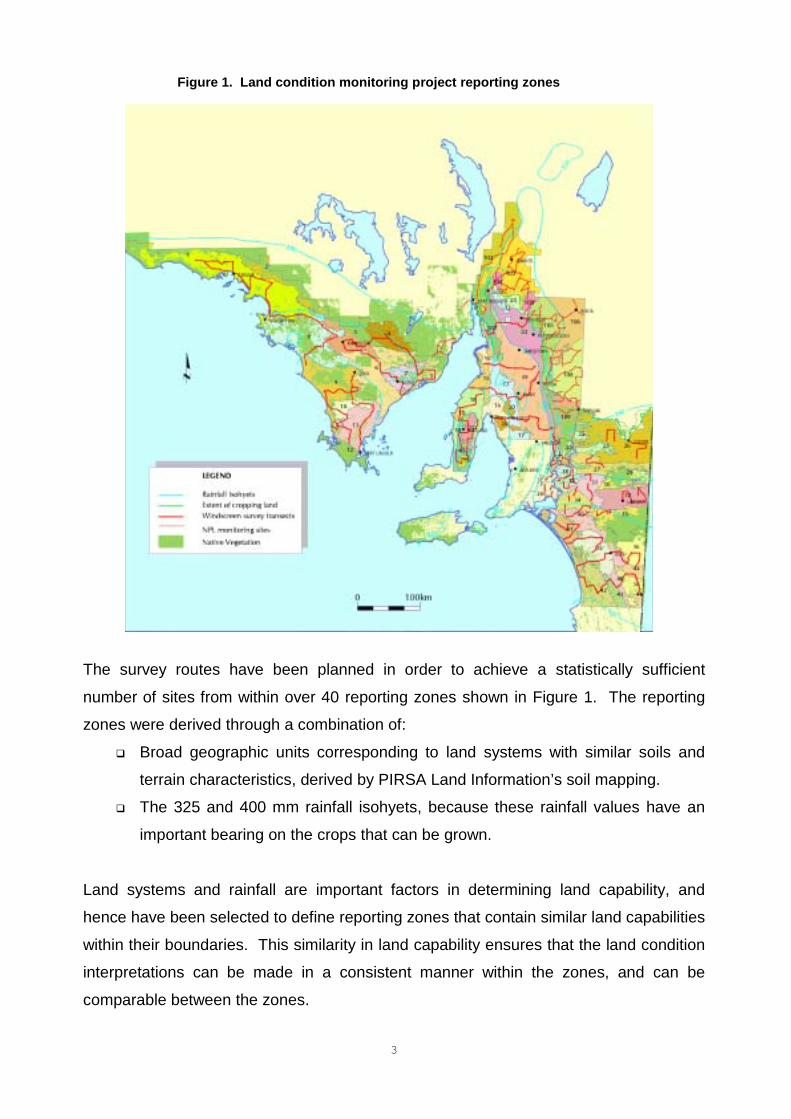
Figure 1. Land condition monitoring project reporting zones
The survey routes have been planned in order to achieve a statistically sufficient
number of sites from within over 40 reporting zones shown in Figure 1. The reporting
zones were derived through a combination of:
� Broad geographic units corresponding to land systems with similar soils and
terrain characteristics, derived by PIRSA Land Information’s soil mapping.
� The 325 and 400 mm rainfall isohyets, because these rainfall values have an
important bearing on the crops that can be grown.
Land systems and rainfall are important factors in determining land capability, and
hence have been selected to define reporting zones that contain similar land capabilities
within their boundaries. This similarity in land capability ensures that the land condition
interpretations can be made in a consistent manner within the zones, and can be
comparable between the zones.
4
Several drawbacks have been identified in the windscreen survey methodology.
Although difficult to quantify, it is anticipated that these problems are likely to result in
biases and inconsistencies in the resulting survey dataset. The key issues in this
respect include:
� survey sites being confined to roadside paddocks with difficult to reach areas
not being surveyed at all;
� inconsistencies in survey timing and surveys being done during slightly different
cropping stages in some areas;
� the large number of trained observers for extended periods results in high
operating costs and logistical effort; and
� likely inconsistencies in sampling standards between different observers.
The LCMP achieves its goals through monitoring a number of key indicators of land
condition. These include:
� wind erosion;
� water erosion;
� non-pastoral lease rangelands vegetation;
� soil acidity;
� soil salinity;
� soil structure decline;
� soil fertility; and
� water repellence.
Once fully investigated, it is anticipated that remote sensing will provide the opportunity
to conduct more advanced and improved land condition monitoring than possible
through a sole reliance on the current windscreen survey methodology.
This report is concerned with a series of investigations that were conducted to evaluate
these expected benefits in support of the on-going LCMP efforts. The work of this study
focussed on the following key issues associated with land condition in this State:
� water erosion (mixed agriculture areas);
� wind erosion (mixed agriculture areas);
� NLPR vegetation and erosion; and
� dryland salinity.

5
The report is laid out in the following sections:
� Section 1 – overview of remote sensing technology;
� Section 2 – erosion (water and wind) in the mixed cropping areas;
� Section 3 – NPLR vegetation condition;
� Section 4 – dryland salinity; and finally
� Section 5 –conclusions and recommendations.
6
SECTION 1: REMOTE SENSING FOR PROJECTSThis section provides an overview of remote sensing, particularly as it relates to natural
resources management and agricultural applications. Some important principles
involved in the use of the various technologies are presented - although Appendix 1
contains a more detailed discussion on remote sensing, and covers issues such as the
physics of remote sensing and issues of scale and image quality. This section also
contains a description of the remote sensing systems used during the course of the
study.
1.1 The “lure” of remote sensingOne of the key benefits of many remote sensing systems used in natural resources
projects lies in the fact that large areas of land can be covered instantaneously and
repeatedly. In most cases the methodologies that are used already exist, are
operational, and are standardised to ensure repeatability and consistency in the results
- remote sensing is now a “mature” technology.
Although the cost of the imagery may initially be quite expensive, the ability to cover
large land areas often makes them extremely cost-effective. In determining cost-
effectiveness, it is important to reconcile image costs with the inherent value of the
activity / land use being assessed or monitored. For example, the use of remote
sensing in projects involving land uses which yield a high return per hectare (e.g.
viticulture and irrigation) are likely to prove more cost-effective than low yielding land
uses like extensive rangeland grazing. These considerations are important when
determining the viability of remote sensing in natural resources projects, especially
when considering the role for these technologies in on-going, long-term monitoring
projects.
The fixed orbit repeatability of many satellite-based remote sensing systems ensure that
imagery is up-dated on a regular basis. Orbit intervals of conventionally used satellite
systems range from twice daily (e.g. NOAA) to approximately twice monthly (Landsat),
thus making them ideal for multitemporal, change detection and monitoring applications.
Although most satellite-based remote sensing systems orbit on a regular basis, their
timing is fixed making them unsuitable in applications such as monitoring disasters (e.g.
locust plague, flood monitoring) or capturing area coverages at critical and short-lived
phases (e.g. algal blooms, maximum crop vigour). Further, because many of the
7
remote sensing systems used cannot penetrate cloud, image acquisitions may be totally
obscured at the time of critical overpasses. By way of contrast, airborne-based remote
sensing can prove to be extremely user-friendly with respect to ad hoc acquisitions,
often making them ideal where timing and high image qualities are critical to the
outcomes of the project. Indeed, some airborne remote sensing methodologies, e.g.
video remote sensing (VRS) and airborne digital photography (ADP) are sufficiently low-
tech. to enable resource managers themselves to configure and fly their own systems to
suit unique project needs in terms of image timing and resolution (Thomas, 1997). VRS
and ADP are discussed in detail further in this document.
Remotely sensed images are conventionally supplied in digital formats that are readily
fed into computers for classification work using digital image processing techniques. As
eluded to earlier in the document, the key advantage of classifying through image
processing are that images can be classified quickly, consistently and objectively using
the standardised routines. These attributes are essential in successful change
detection and monitoring projects. The high processing power, storage capacity and
falling prices of the current generation of PC’s means that image processing is
becoming increasingly attractive and cost-effective.
1.2 Satellite-based remote sensingChoosing between various types of satellite imagery in a project is achieved by carefully
considering the specific information requirements of the project (e.g. scale, mapping
themes, timing and frequency, cost, etc..) and matching these as best as possible with
the capabilities of the various satellites systems that are available. Currently the most
commonly used mid resolution remote sensing systems are on-board the Landsat and
SPOT satellites. These remote sensing systems have consistently proven their worth in
natural resources applications and can be considered the “work horses” of the suite of
conventional remote sensing systems that are on offer. These systems have been
specifically designed to focus on providing information on soils, rocks and vegetation.
The middle resolutions provided through Landsat and SPOT make them ideal for
application at scales ranging from paddock to landscape scales (i.e. 1: 40,000 to 1:
100,000). Table 1 presents the important benefits of these satellite systems in natural
resources projects. The following sections present the key attributes of these satellites
and their imagery.
8
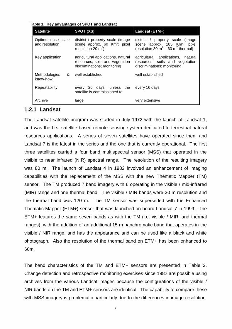
Table 1. Key advantages of SPOT and Landsat
Satellite SPOT (XS) Landsat (ETM+)
Optimum use scaleand resolution
district / property scale (imagescene approx. 60 Km2; pixelresolution 20 m2)
district / property scale (imagescene approx. 185 Km2; pixelresolution 30 m2 – 60 m2 thermal)
Key application agricultural applications, naturalresources; soils and vegetationdiscriminations; monitoring
agricultural applications, naturalresources; soils and vegetationdiscriminations; monitoring
Methodologies &know-how
well established well established
Repeatability every 26 days, unless thesatellite is commissioned to
every 16 days
Archive large very extensive
1.2.1 Landsat
The Landsat satellite program was started in July 1972 with the launch of Landsat 1,
and was the first satellite-based remote sensing system dedicated to terrestrial natural
resources applications. A series of seven satellites have operated since then, and
Landsat 7 is the latest in the series and the one that is currently operational. The first
three satellites carried a four band multispectral sensor (MSS) that operated in the
visible to near infrared (NIR) spectral range. The resolution of the resulting imagery
was 80 m. The launch of Landsat 4 in 1982 involved an enhancement of imaging
capabilities with the replacement of the MSS with the new Thematic Mapper (TM)
sensor. The TM produced 7 band imagery with 6 operating in the visible / mid-infrared
(MIR) range and one thermal band. The visible / MIR bands were 30 m resolution and
the thermal band was 120 m. The TM sensor was superseded with the Enhanced
Thematic Mapper (ETM+) sensor that was launched on board Landsat 7 in 1999. The
ETM+ features the same seven bands as with the TM (i.e. visible / MIR, and thermal
ranges), with the addition of an additional 15 m panchromatic band that operates in the
visible / NIR range, and has the appearance and can be used like a black and white
photograph. Also the resolution of the thermal band on ETM+ has been enhanced to
60m.
The band characteristics of the TM and ETM+ sensors are presented in Table 2.
Change detection and retrospective monitoring exercises since 1982 are possible using
archives from the various Landsat images because the configurations of the visible /
NIR bands on the TM and ETM+ sensors are identical. The capability to compare these
with MSS imagery is problematic particularly due to the differences in image resolution.
9
A large global Landsat archive exists and can be accessed without difficulty either from
Australian sources or from overseas.
Landsat 7 is operated on a cost recovery basis. The previous Landsat satellites were
commercialised - as future ones might be.
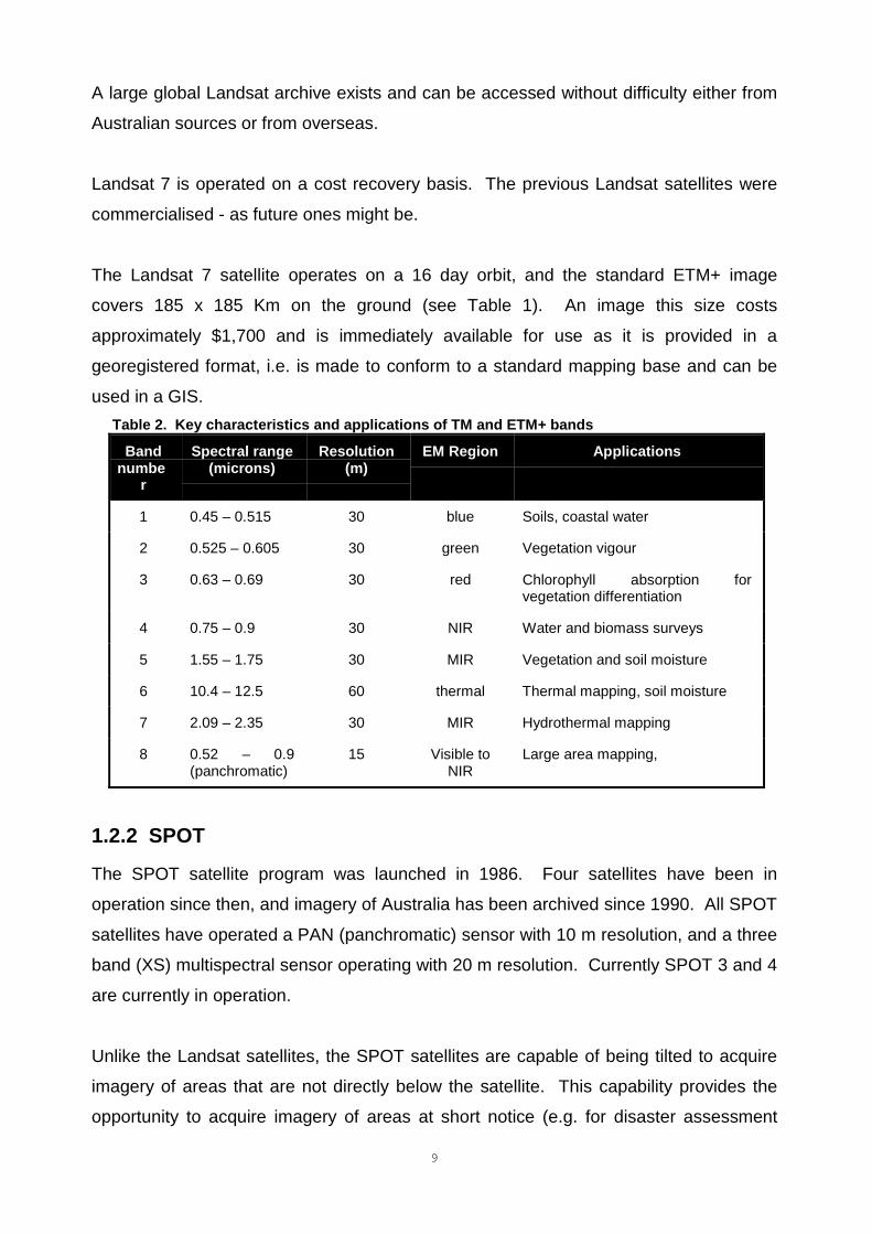
The Landsat 7 satellite operates on a 16 day orbit, and the standard ETM+ image
covers 185 x 185 Km on the ground (see Table 1). An image this size costs
approximately $1,700 and is immediately available for use as it is provided in a
georegistered format, i.e. is made to conform to a standard mapping base and can be
used in a GIS.Table 2. Key characteristics and applications of TM and ETM+ bands
Bandnumbe
r
Spectral range(microns)
Resolution(m)
EM Region Applications
1 0.45 – 0.515 30 blue Soils, coastal water
2 0.525 – 0.605 30 green Vegetation vigour
3 0.63 – 0.69 30 red Chlorophyll absorption forvegetation differentiation
4 0.75 – 0.9 30 NIR Water and biomass surveys
5 1.55 – 1.75 30 MIR Vegetation and soil moisture
6 10.4 – 12.5 60 thermal Thermal mapping, soil moisture
7 2.09 – 2.35 30 MIR Hydrothermal mapping
8 0.52 – 0.9(panchromatic)
15 Visible toNIR
Large area mapping,
1.2.2 SPOT
The SPOT satellite program was launched in 1986. Four satellites have been in
operation since then, and imagery of Australia has been archived since 1990. All SPOT
satellites have operated a PAN (panchromatic) sensor with 10 m resolution, and a three
band (XS) multispectral sensor operating with 20 m resolution. Currently SPOT 3 and 4
are currently in operation.
Unlike the Landsat satellites, the SPOT satellites are capable of being tilted to acquire
imagery of areas that are not directly below the satellite. This capability provides the
opportunity to acquire imagery of areas at short notice (e.g. for disaster assessment
10
applications) or for taking advantage of weather breaks i.e. for studies in areas that are
often obscured by clouds during critical project phases. The normal orbit interval of the
SPOT satellite is every 26 days. However, as the orbits of SPOTs 3 and 4 have been
configured so that they each operate in orbits half a cycle apart, routine SPOT
acquisitions are available every 13 days – although much shorter if the satellites are
tilted.
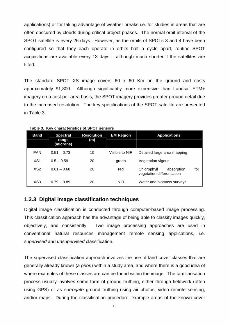
The standard SPOT XS image covers 60 x 60 Km on the ground and costs
approximately $1,800. Although significantly more expensive than Landsat ETM+
imagery on a cost per area basis, the SPOT imagery provides greater ground detail due
to the increased resolution. The key specifications of the SPOT satellite are presented
in Table 3.
Table 3. Key characteristics of SPOT sensors
Band Spectralrange
(microns)
Resolution(m)
EM Region Applications
PAN 0.51 – 0.73 10 Visible to NIR Detailed large area mapping
XS1 0.5 – 0.59 20 green Vegetation vigour
XS2 0.61 – 0.68 20 red Chlorophyll absorption forvegetation differentiation
XS3 0.79 – 0.89 20 NIR Water and biomass surveys
1.2.3 Digital image classification techniques
Digital image classification is conducted through computer-based image processing.
This classification approach has the advantage of being able to classify images quickly,
objectively, and consistently. Two image processing approaches are used in
conventional natural resources management remote sensing applications, i.e.
supervised and unsupervised classification.
The supervised classification approach involves the use of land cover classes that are
generally already known (a priori) within a study area, and where there is a good idea of
where examples of these classes are can be found within the image. The familiarisation
process usually involves some form of ground truthing, either through fieldwork (often
using GPS) or as surrogate ground truthing using air photos, video remote sensing,
and/or maps. During the classification procedure, example areas of the known cover
11
classes are located within the image and are used as “training sets”. Training sets
contain unique spectral information (“spectral signatures”) of the sought after cover
class, and are used to locate other similar areas in the imagery by analysing their
spectral signatures. Ideally, a number of training sets should be selected per cover
class during training. This is done to take into account the intra-cover class variability in
the class spectra due to the differing influences of background soils, condition,
landscape location, illumination, moisture, etc., with the premise being that the spread is
statistically “normal”. Once the classification is underway the computer carries out a
statistically based analysis to match all pixels within an image into the desired classes
that were defined during the training procedure. Pre-determined thresholds and various
other inputs are predefined in the classification parameters to resolve the classification
of spectrally confusing image areas.
The unsupervised classifications procedure has less human input / is more computer-
automated than the supervised approach. Unsupervised classifications are suited to
situations in which the user is either unfamiliar with the cover classes within a study
area, or is unable to locate reliable training sets within the image due to lack of suitable
ground truthing information. The procedure requires user input to define the
classification parameters, which include the number of desired output classes required
and the statistical approach to the classification. Once the process is underway, the
computer sorts the whole of the image into the predefined number of classes, based on
the discreteness of their spectra. If the predefined number of classes is sufficiently
large, it is likely that some land cover classes (e.g. pasture, wooded classes) contain a
number of the output classes, whereas too few predetermined classes will result in land
cover classes being merged. For this reason it is usual to predefine a large number of
output classes (e.g. 30 to 50) in the classification parameters which can be sorted and
merged into meaningful land cover classes with the support of local knowledge.
Supervised classifications are most suited to situations where the user has a good prior
understanding of the classes that exist, where good ground truth data is available, and
where the study area is heterogeneous, e.g. land cover mapping applications.
Unsupervised classifications, however, are most suited to situations where the user may
be unfamiliar with the study area, or where the scene is homogeneous, or where the
desired classes reflect variations within land cover class. For example, unsupervised
classifications are ideal for mapping geological mineral alterations, crop stress, or
12
different land uses (e.g. the mixed cropping, horticulture, improved pasture land uses of
the agricultural land cover class). In many cases it is effective to use both techniques in
sequence. For example, a preliminary unsupervised classification can be effective in
gaining a familiarity of a study area and / or in removing from the image areas that are
unwanted in the final classification to make the following supervised classification faster
and more efficient.
1.3 Airborne remote sensing systemsAs has been discussed earlier, satellite-based remote sensing is ideally suited to small
scale, large area natural resource management applications, e.g.:
� regional and “property” scales (e.g. 1: 100,000) - with Landsat, and
� “paddock” scale (e.g. 1: 40,000) - with SPOT.
Airborne remote sensing provides imagery with greater resolution than available from
satellite remote sensing imagery. For example, airborne systems typically provide
imagery with ground resolutions that range between 5 m to 30 cm, and are suited to
application at scales that range between 1: 2,500 and 1: 250. At these types of scales
users have the opportunity to use airborne imagery in, for example, soil conservation
and habitat type applications which high ground detail is required. In this sense, the
types of applications that airborne remote sensing are most suited fits between the
broadscale applications from satellite remote sensing and the analysis scales that are
achievable through fieldwork; airborne remote sensing bridges the scale gap between
the two.
For the purposes of this report the term “airborne remote sensing” focuses on three
different systems investigated during the study. These include:
� video remote sensing (VRS);
� airborne digital photography (ADP); and
� digital multispectral video system called “Digital MultiSpectral Video” (DMSV).
VRS and ADP are notable in terms of the various remote sensing systems commonly
on offer for their reliance on low tech. and easily accessible technologies. These
systems almost always configured and operated by natural resource managers
themselves in order to satisfy particular project requirements, often driven by factors
such as timing, scale and budget. For example Mr Iain Grierson of the Adelaide
13
University Department of Soil and Water was instrumental in the development of the
VRS and ADP systems used throughout the course of this study, and are more fully
described in Section 2.4.2. The generic systems used are generally configured around
readily available, off-the-shelf components, and often include the following in
combination:
� digital or video cameras,
� GPS units, usually hand-held types,
� caption generators,
� camera mountings, and
� laptop computers.
Costs are further reduced through operating these systems on board low flying cost light
aircraft that require minimal modification to host the equipment on board.
The VRS and ADP used during the course of the study were georeferenced through
linking the imagery with simultaneously acquired GPS data. The capability to perform
georegistration is important for uses that require the ability to either:
� locate airborne remote sensing in the field for ground truthing;
� co-register airborne remote sensing with satellite images whereby the airborne
remote sensing is used surrogate ground truthing; or for
� co-registering airborne remote sensing with other coverages within a GIS.
Each of the three airborne remote sensing systems briefly described above produce
high quality images that can be presented through standard PCs and image processing
/ graphics software. The various images can be analysed on screen or printed using
high quality colour printers for subsequent air photo interpretation (API), or digitally
classified through the methods discussed in Section 1.2.3.
The following sections provide an overview of the VRS, ADP and DMSV systems used
during the study. These also discusses in detail the VRS and ADP system
configurations that were used as part of the work conducted in the cropping areas
(Section 2) and the NPLR areas (Section 3).
1.3.1 VRS system overview
In essence, VRS involves recording continuous imagery of the aircraft’s flightline on
videotape using commonly used video formats (VHS, S-VHS and Hi-8). The capability
14
to record sound and vision simultaneously enables in flight commentary to be recorded
which for subsequent playback to aid in interpretations. Once a project area is located
on the video tape, the area can be moving image can be “frozen” and converted into an
image frame (digital image file) through a process known as “framegrabbing”.
The key components of Adelaide University’s VRS system include the following:
� Cessna 172 light aircraft;
� camera mounting;
� video camera and recording device;
� GPS; and
� video monitors.
Cessna 172 light aircraft:- The Cessna 172 is an ideal aircraft for this type of work
because of its low running costs, good range and flight stability. The wing slung
fuselage configuration ensures excellent stability and the aircraft is large enough to
accommodate up to four people during a survey. In flight a technician operates the
equipment and records and monitors the performance of the system.
A technician may also support the navigation through the use of a laptop-based
program called “Sky Trek” which was developed for the University by Ken Fox of
Burnside Programming Ltd. in Adelaide. The Sky Trek overlays the flightline in real time
by interfacing with a GPS over a georegistered backdrop (scanned air photos, maps or
satellite imagery) of the survey area containing waypoints, roads and other information
to help in successful navigation.
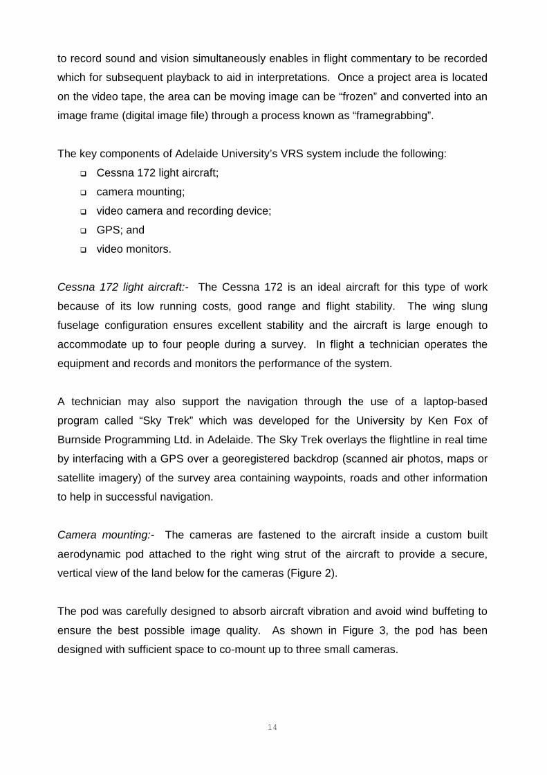
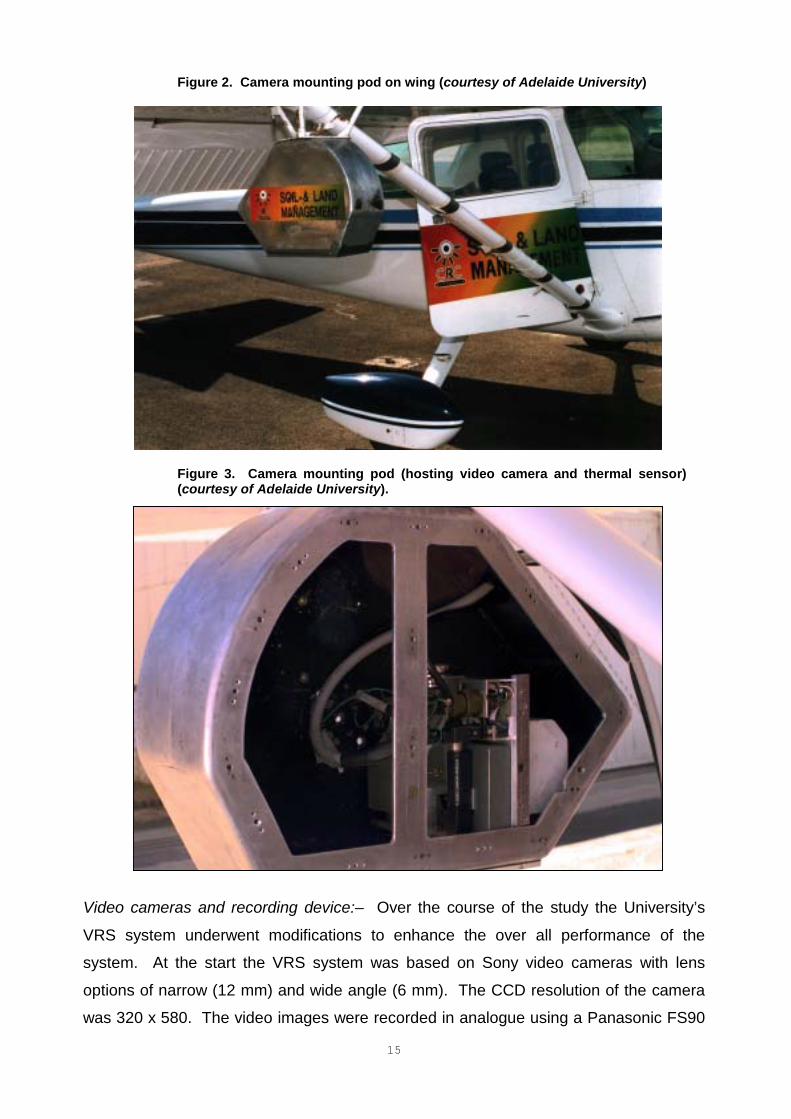
Camera mounting:- The cameras are fastened to the aircraft inside a custom built
aerodynamic pod attached to the right wing strut of the aircraft to provide a secure,
vertical view of the land below for the cameras (Figure 2).
The pod was carefully designed to absorb aircraft vibration and avoid wind buffeting to
ensure the best possible image quality. As shown in Figure 3, the pod has been
designed with sufficient space to co-mount up to three small cameras.
15
Figure 2. Camera mounting pod on wing (courtesy of Adelaide University)
Figure 3. Camera mounting pod (hosting video camera and thermal sensor)(courtesy of Adelaide University).
Video cameras and recording device:– Over the course of the study the University’s
VRS system underwent modifications to enhance the over all performance of the
system. At the start the VRS system was based on Sony video cameras with lens
options of narrow (12 mm) and wide angle (6 mm). The CCD resolution of the camera
was 320 x 580. The video images were recorded in analogue using a Panasonic FS90
16
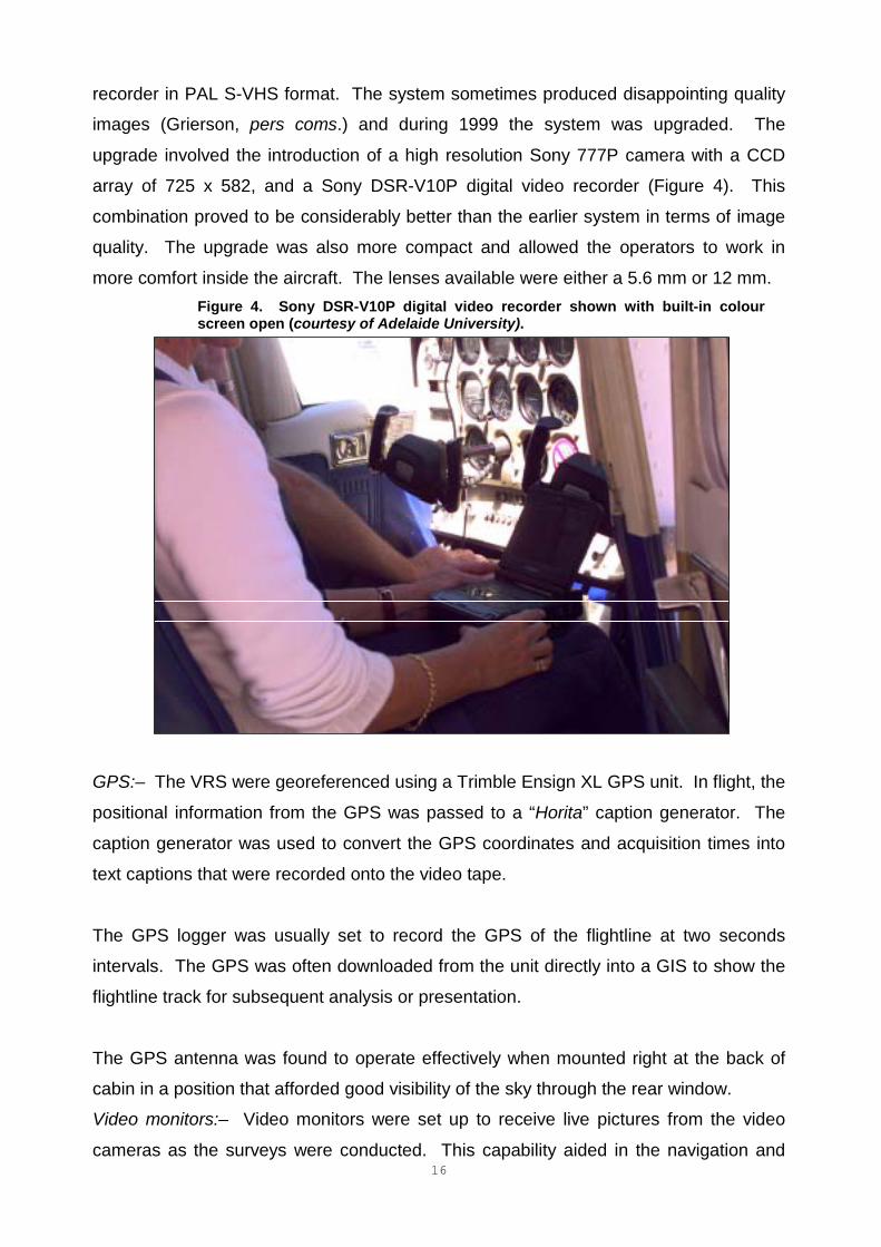
recorder in PAL S-VHS format. The system sometimes produced disappointing quality
images (Grierson, pers coms.) and during 1999 the system was upgraded. The
upgrade involved the introduction of a high resolution Sony 777P camera with a CCD
array of 725 x 582, and a Sony DSR-V10P digital video recorder (Figure 4). This
combination proved to be considerably better than the earlier system in terms of image
quality. The upgrade was also more compact and allowed the operators to work in
more comfort inside the aircraft. The lenses available were either a 5.6 mm or 12 mm.Figure 4. Sony DSR-V10P digital video recorder shown with built-in colourscreen open (courtesy of Adelaide University).
GPS:– The VRS were georeferenced using a Trimble Ensign XL GPS unit. In flight, the
positional information from the GPS was passed to a “Horita” caption generator. The
caption generator was used to convert the GPS coordinates and acquisition times into
text captions that were recorded onto the video tape.
The GPS logger was usually set to record the GPS of the flightline at two seconds
intervals. The GPS was often downloaded from the unit directly into a GIS to show the
flightline track for subsequent analysis or presentation.
The GPS antenna was found to operate effectively when mounted right at the back of
cabin in a position that afforded good visibility of the sky through the rear window.
Video monitors:– Video monitors were set up to receive live pictures from the video
cameras as the surveys were conducted. This capability aided in the navigation and
17
also provided the vital check that the cameras were operating well. Initially a small
black & white monitor was used but this superseded when the Sony DSR-V10P digital
video recorder was introduced with its small in-built colour monitor.
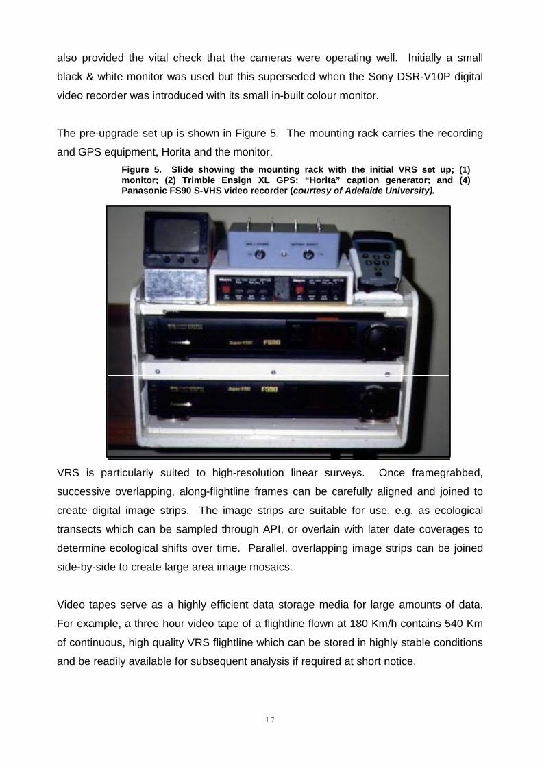
The pre-upgrade set up is shown in Figure 5. The mounting rack carries the recording
and GPS equipment, Horita and the monitor.Figure 5. Slide showing the mounting rack with the initial VRS set up; (1)monitor; (2) Trimble Ensign XL GPS; “Horita” caption generator; and (4)Panasonic FS90 S-VHS video recorder (courtesy of Adelaide University).
VRS is particularly suited to high-resolution linear surveys. Once framegrabbed,
successive overlapping, along-flightline frames can be carefully aligned and joined to
create digital image strips. The image strips are suitable for use, e.g. as ecological
transects which can be sampled through API, or overlain with later date coverages to
determine ecological shifts over time. Parallel, overlapping image strips can be joined
side-by-side to create large area image mosaics.
Video tapes serve as a highly efficient data storage media for large amounts of data.
For example, a three hour video tape of a flightline flown at 180 Km/h contains 540 Km
of continuous, high quality VRS flightline which can be stored in highly stable conditions
and be readily available for subsequent analysis if required at short notice.
18
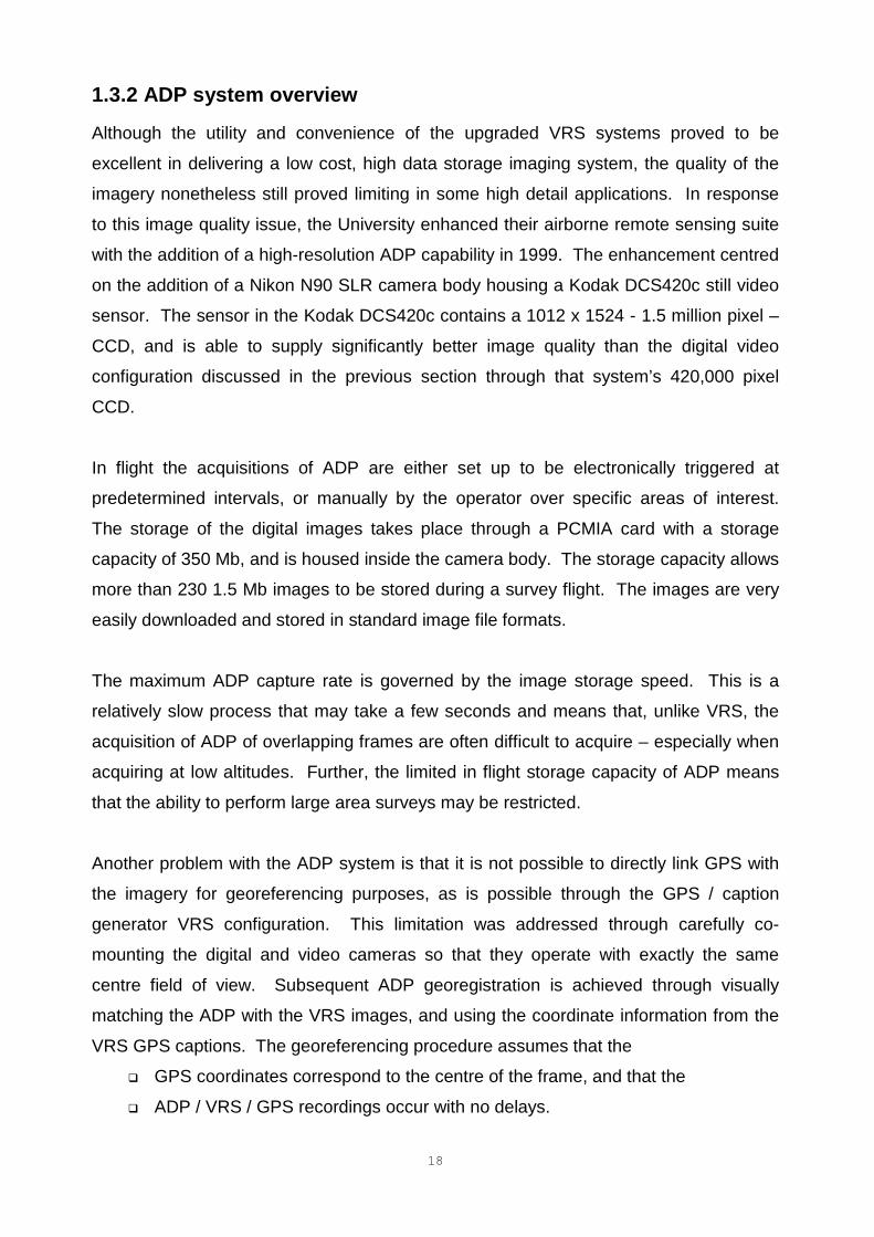
1.3.2 ADP system overview
Although the utility and convenience of the upgraded VRS systems proved to be
excellent in delivering a low cost, high data storage imaging system, the quality of the
imagery nonetheless still proved limiting in some high detail applications. In response
to this image quality issue, the University enhanced their airborne remote sensing suite
with the addition of a high-resolution ADP capability in 1999. The enhancement centred
on the addition of a Nikon N90 SLR camera body housing a Kodak DCS420c still video
sensor. The sensor in the Kodak DCS420c contains a 1012 x 1524 - 1.5 million pixel –
CCD, and is able to supply significantly better image quality than the digital video
configuration discussed in the previous section through that system’s 420,000 pixel
CCD.
In flight the acquisitions of ADP are either set up to be electronically triggered at
predetermined intervals, or manually by the operator over specific areas of interest.
The storage of the digital images takes place through a PCMIA card with a storage
capacity of 350 Mb, and is housed inside the camera body. The storage capacity allows
more than 230 1.5 Mb images to be stored during a survey flight. The images are very
easily downloaded and stored in standard image file formats.
The maximum ADP capture rate is governed by the image storage speed. This is a
relatively slow process that may take a few seconds and means that, unlike VRS, the
acquisition of ADP of overlapping frames are often difficult to acquire – especially when
acquiring at low altitudes. Further, the limited in flight storage capacity of ADP means
that the ability to perform large area surveys may be restricted.
Another problem with the ADP system is that it is not possible to directly link GPS with
the imagery for georeferencing purposes, as is possible through the GPS / caption
generator VRS configuration. This limitation was addressed through carefully co-
mounting the digital and video cameras so that they operate with exactly the same
centre field of view. Subsequent ADP georegistration is achieved through visually
matching the ADP with the VRS images, and using the coordinate information from the
VRS GPS captions. The georeferencing procedure assumes that the
� GPS coordinates correspond to the centre of the frame, and that the
� ADP / VRS / GPS recordings occur with no delays.
19
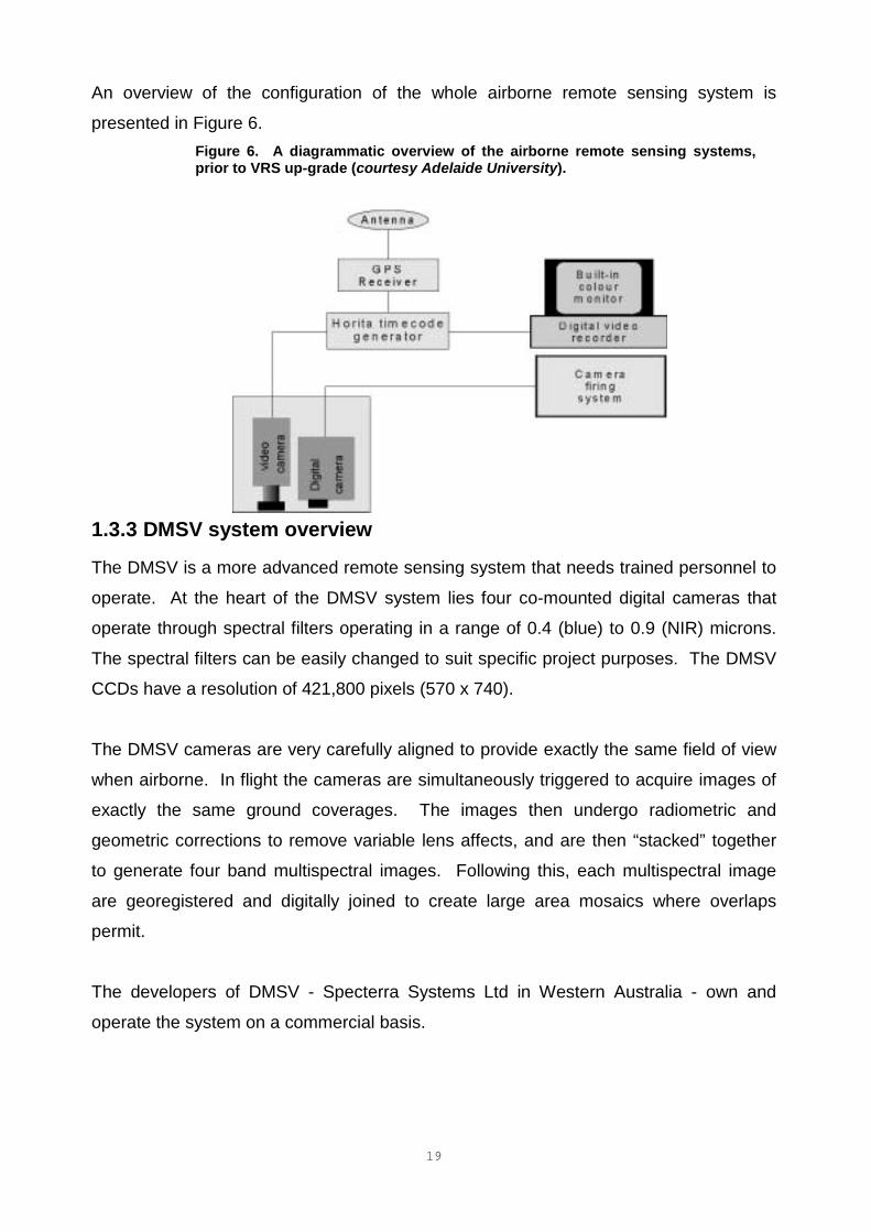
An overview of the configuration of the whole airborne remote sensing system is
presented in Figure 6.Figure 6. A diagrammatic overview of the airborne remote sensing systems,prior to VRS up-grade (courtesy Adelaide University).
1.3.3 DMSV system overview
The DMSV is a more advanced remote sensing system that needs trained personnel to
operate. At the heart of the DMSV system lies four co-mounted digital cameras that
operate through spectral filters operating in a range of 0.4 (blue) to 0.9 (NIR) microns.
The spectral filters can be easily changed to suit specific project purposes. The DMSV
CCDs have a resolution of 421,800 pixels (570 x 740).
The DMSV cameras are very carefully aligned to provide exactly the same field of view
when airborne. In flight the cameras are simultaneously triggered to acquire images of
exactly the same ground coverages. The images then undergo radiometric and
geometric corrections to remove variable lens affects, and are then “stacked” together
to generate four band multispectral images. Following this, each multispectral image
are georegistered and digitally joined to create large area mosaics where overlaps
permit.
The developers of DMSV - Specterra Systems Ltd in Western Australia - own and
operate the system on a commercial basis.
20
SECTION 2: EROSION SUSCEPTIBILITY IN MIXEDCROPPING DISTRICTS
This section presents the work conducted to develop a soil erosion susceptibility
modelling methodology that can be applied to provide a consistency in approach and
results over time.
2.1 Overview of erosion in cropping areasSoil erosion is a natural and on-going process that shapes our landscapes. In non-
degraded, pristine landscapes the rate of soil loss is usually balanced by the rate of soil
formation to ensure the maintenance of very low erosion susceptibilities. The presence
of natural vegetation plays a vital role in protecting the soil surface from erosion.
However, when the ground cover is cleared and land use changed (e.g. when land is
cleared for agriculture), the equilibrium is invariably altered, often leading to
unsustainable erosion rates unless careful land management practices are adopted.
This is especially the situation in cropped areas that undergo large fluctuations in
erosion susceptibilities – particularly when the land first undergoes clearance, and then
annually during the cultivation phase.
Soil erosion is an insidious process that strongly impacts on agricultural sustainability
due to losses of nutrients and soil microbial activity, reduced effective rooting depth and
soil water infiltration rates. On the one hand it can lead to reduced soil water
availability, whilst on the other hand, erosion may contribute to reduced water-use
efficiency and rising groundwater, which may lead to dryland salinity, sodicity, and / or
acid sulfate soils. Sand blasting during wind erosion events may deliver significant
damage to young crops, and affect the capacity of effected plants to combat disease,
flower and set grain. In the case of water erosion, the downstream environmental
impacts can be severe because of reduced water quality (e.g. turbidity and mobilisation
of soil / regolith salts and chemicals) and the siltation of watercourses and reservoirs
leading to a reduced environmental capacity to moderate stream flows. Soil erosion
therefore represents a vitally important land degradation issue within South Australia as
it has wide reaching consequences with respect to the State’s agricultural sustainability
and environmental health. The scale and prominence of the erosion problem is strongly
reflected in the overall effort of the LCMP.
Since most erosion is ephemeral and difficult to detect once crops are established, the
aim of this work was focused on developing monitoring techniques for erosion
21
susceptibility. Principally, this means using remote sensing to assess soil cover
exposure during peak exposure, i.e. the time when largest total area of (bare) soils are
in their most vulnerable state with respect to wind or water erosion. This time coincides
with the short period between paddock cultivation and the establishment of sufficiently
protective crop covers, i.e. any time between April and July in South Australia. Where
appropriate, the remote sensing-derived cover data were incorporated into a GIS for
erosion modelling. To that end, trials were conducted to evaluate the potential roles of
SPOT XS and airborne remote sensing (VRS and digital photography) in supporting
erosion monitoring work in the cropping areas, and are discussed further in the following
sections.
2.2 SPOT satellite in cropping areasErosion remains the most important contributor to land degradation in the cropping
areas of South Australia (Figure 8). It is for this reason that the LCMP concentrates a
great deal of effort in monitoring erosion indicators through the windscreen survey work.
The main aim of the project is to monitor erosion risk by assessing soil cover exposure,
and to this end a rudimentary Erosion Hazard Index was developed by the LCMP to
monitor key indicators including, soil surface texture, residue detachment (for wind
erosion), and slope (for water erosion). A key erosion risk indicator measured by the
LCMP is the area of unprotected land during peak exposure.
This section discusses an evaluation of remote sensing and GIS modelling in
determining erosion susceptibility during peak exposure in 1999 and 2000, and
demonstrates the methodology in susceptibility change detection between the two
years. The interest in this approach lies in the desire for the LCMP to achieve:
� greater cost-efficiencies;
� faster information turnaround times;
� increased consistency / reduced subjectivity; and
� consistently produced regional maps for all areas.
The combination of remote sensing and GIS modelling has been used successfully in
erosion studies, e.g. Lantieri et al (1990), Flavel (1990), Jäger (1992), De Jong (1994),
Cyr et al (1995) and Thomas (2000). This approach exploits the capability of
combining, through GIS modelling, timely soil cover data derived through remote
22
sensing with various environmental / landscape variables that influence soil erosion,
e.g. soil texture, landscape, land use, and climate.
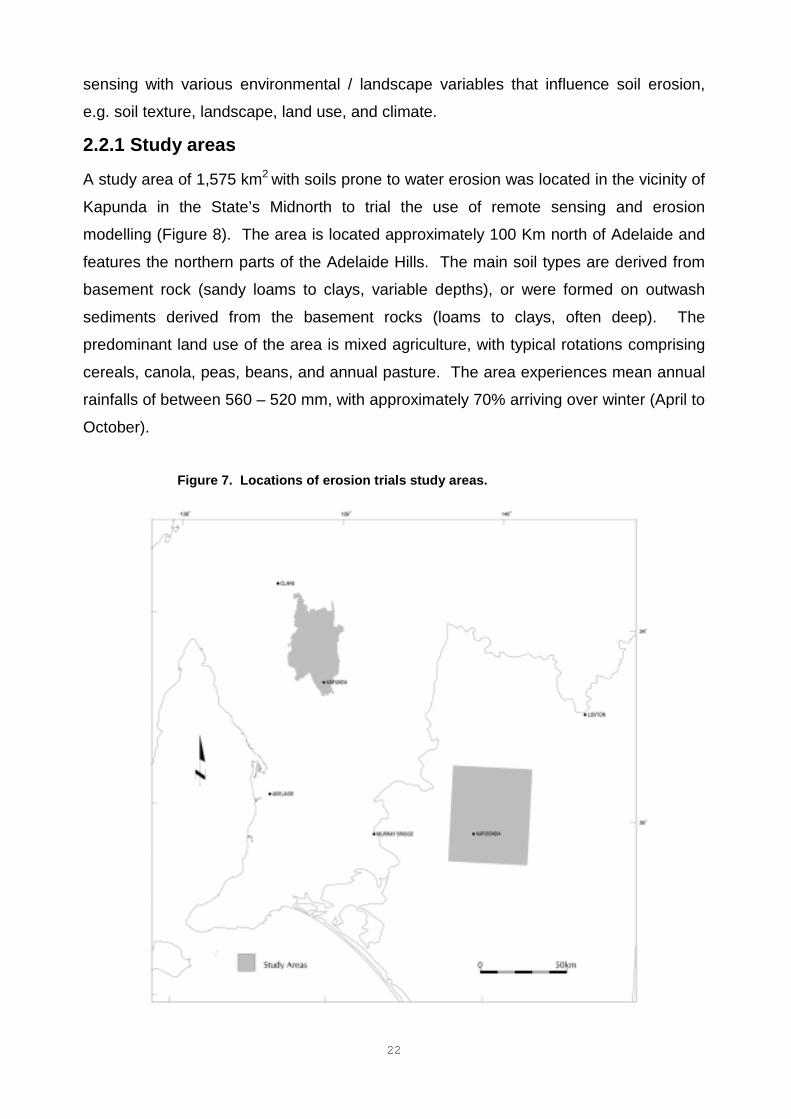
2.2.1 Study areas
A study area of 1,575 km2 with soils prone to water erosion was located in the vicinity of
Kapunda in the State’s Midnorth to trial the use of remote sensing and erosion
modelling (Figure 8). The area is located approximately 100 Km north of Adelaide and
features the northern parts of the Adelaide Hills. The main soil types are derived from
basement rock (sandy loams to clays, variable depths), or were formed on outwash
sediments derived from the basement rocks (loams to clays, often deep). The
predominant land use of the area is mixed agriculture, with typical rotations comprising
cereals, canola, peas, beans, and annual pasture. The area experiences mean annual
rainfalls of between 560 – 520 mm, with approximately 70% arriving over winter (April to
October).
Figure 7. Locations of erosion trials study areas.
23
A study area for the wind erosion modelling trials was located in the vicinity of Karoonda
in the Murray Mallee, approximately 150 km east of Adelaide (Figure 7). This area
covers 1,760 km2 and is dominated by a landscape of aeolian dune systems featuring
sands and on the dunes sandy loams in the inter-dune areas. The western section of
the study area is dominated by plains and rises with shallow loams, often containing a
high proportion of calcrete stones. The dune systems are oriented tangentially to the
prevailing
northeasterly and southwesterly winds. The main land use is mixed farming with
rotations of cereals and annual pasture, although occasional canola and legume crops
are sometimes grown. The mean annual rainfall is in the range of 310 – 350 mm, with
66% falling during the winter.
2.2.2 Erosion susceptibility modelling
Erosion soil loss models fall into one of two categories. They are either:
� process-based models that seek to represent, through mathematical formulae,
the mechanical processes at play during erosion events (usually in terms of
kinetic energies), or
� empirical models that calibrate the influence of the landscape and
environmental variables involved in erosion through the regression analysis of
large numbers of field observations from erosion trials.
Building process-based models requires a large investment in research to understand
and model the precise processes involved in erosion. Empirical models require large
quantities of erosion field data, and are somewhat limited in where they may be applied
without undergoing rigorous calibration in new areas.
According to Lantieri et al (1990), erosion models seek to predict or estimate soil
volume losses, whereas erosion susceptibility models seek to determine the risk of
erosion under certain scenarios, e.g. “a one in 50 year” occurrence of rainfall or wind, or
a change in land use. Erosion susceptibility is presented in relative values that rank the
erosion risk under the given scenarios. In this study, the scenario was taken as the time
of peak exposure when South Australia faces its greatest potential erosion liability.
24
2.2.3 Water erosion susceptibility modelling
The Universal Soil Loss Equation (USLE) is an empirically-based water erosion soil loss
model developed from thousands of field trials conducted in catchments in the USA.
Numerous detailed descriptions of the USLE are available elsewhere, e.g. in
Wischmeier and Smith (1978), Hudson (1981), and USDA (1997). In essence, the
USLE seeks to isolate the key variables in the environment and landscape that govern
water erosion (so-called “USLE factors”) on a given slope, and reduce these to a
numeric value referenced from look up tables.
A soil loss for the slope is generated when the factor values are multiplied together in
the USLE equation:
A = R K (L S) C P
where:
A = the computed soil loss per area per year;
R = the rainfall factor;
K = the soil erodibility factor;
(L S) = the combined slope length (L) and slope angle (S) factors;
C = the soil cover factor; and
P = the support (conservation) factor.
Although the USLE was originally devised to enable localised, soil loss calculations in
relation to slope, it has also been adapted to simultaneously map soil erosion
susceptibilities over large areas (Jäger (1992). The study presented here utilised
remote sensing and image processing to derive up-to-date C factors in a similar
approach to Flavel (1990). The other factor values used in the calculation were derived
in the following ways:
� K factors: estimated by combining (1) the soil textures from PIRSA’s 1: 100,000
scale Soil Landscape Unit (SLU) maps with (2) the soil erodibility nomograph in
Hudson (1981). The final factor values for each soil were calibrated against
comparable soils in New South Wales (pers. comms. Rosewell, 1999).
25
� L S factors: sourced from a 20 m resolution digital terrain model (DTM) generated
from 1: 50,000 scale topographic mapping (10 m contours and spot heights). The
20 m resolution was selected to be consistent with the SPOT imagery resolution.
The S component was derived through GIS modelling of the DTM, and the L was set
at 20 m, i.e. the resolution of the DTM. LS factor values were sourced from USDA
(1997).
On investigation of the available data it was discovered that little variability in the R
factor existed across the study area so it was decided not to apply this data in the
calculation. No P factors were used because of the infrequent use of soil conservation
measures in the study area.
2.2.4 Wind erosion susceptibility modelling
To date, research into wind erosion modelling is not as advanced as is the case with
water erosion. This is attributed to an incomplete knowledge of the complicated
processes and interactions that take place during wind erosion events, as required in
the development of process models. Further, the very large amounts of field data
required to create empirical models often makes these models prohibitively expensive
to build (Hudson, 1981). It is only in the last 15 years that there has been real effort
applied to wind erosion modelling e.g. the Wind Erosion Assessment Model (WEAM) in
Shao and Leys (1997).
In the absence of any robust and adaptable models, a model for wind erosion
susceptibility (WES) was developed during the project. Similarly to the USLE, the WES
was designed around on the accumulation of variables in environment and landscape
circumstances that have an important influence on wind erosion.
The WES modelling was performed by co-registering GIS layers representing the
spatial distribution of the variables, and computing erosion susceptibilities using a GIS.
Expert knowledge was used to derive the erosion variables, and their rankings were
based on their level of contribution in the erosion process. The WES model equation is
presented as:
S = T +A + C + E
where:
26
S = wind erosion susceptibility;
T = exposed areas in the landscape topography, i.e. dune tops;
A = slope aspect for exposure to prevailing winds;
C = ground cover; and
E = soil erosivity.
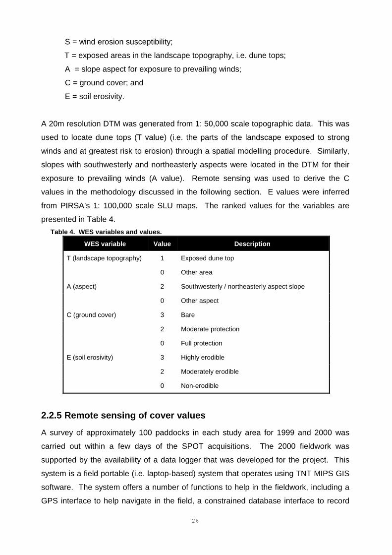
A 20m resolution DTM was generated from 1: 50,000 scale topographic data. This was
used to locate dune tops (T value) (i.e. the parts of the landscape exposed to strong
winds and at greatest risk to erosion) through a spatial modelling procedure. Similarly,
slopes with southwesterly and northeasterly aspects were located in the DTM for their
exposure to prevailing winds (A value). Remote sensing was used to derive the C
values in the methodology discussed in the following section. E values were inferred
from PIRSA’s 1: 100,000 scale SLU maps. The ranked values for the variables are
presented in Table 4.Table 4. WES variables and values.
WES variable Value Description
1 Exposed dune topT (landscape topography)
0 Other area
2 Southwesterly / northeasterly aspect slopeA (aspect)
0 Other aspect
3 Bare
2 Moderate protection
C (ground cover)
0 Full protection
3 Highly erodible
2 Moderately erodible
E (soil erosivity)
0 Non-erodible
2.2.5 Remote sensing of cover values
A survey of approximately 100 paddocks in each study area for 1999 and 2000 was
carried out within a few days of the SPOT acquisitions. The 2000 fieldwork was
supported by the availability of a data logger that was developed for the project. This
system is a field portable (i.e. laptop-based) system that operates using TNT MIPS GIS
software. The system offers a number of functions to help in the fieldwork, including a
GPS interface to help navigate in the field, a constrained database interface to record
27
field attributes, and a GPS interface to georeference the new record. Once back in the
lab, an easy interface enables data to be quickly downloaded and overlaid on the SPOT
image in preparation for the classification work. The capability to accurately overlay the
field attributes greatly supports the classification work though helping to identify training
sets discussed in Section 1.2.3.
The following attributes / information were recorded in the field:
� cover classes (e.g. eroded, bare cultivated, crop, pasture, or stubble);
� cultivation phase (i.e. cultivated or not);
� cover rating;
� GPS position; and
� a digital photograph of the site.
The cover classes were merged into one of three classes, based on similarities in their
spectral and ground protection characteristics (see Table 4). Pasture and stubble were
merged into a “pasture” class because of recent growth of grasses and weeds in the
stubble paddocks.
USLE C factor values were determined from look-up tables in Moore (1990). All
paddocks were estimated to have 0.5 tonne / Ha of protective surface cover either in the
form of residue on bare paddocks or green matter in germinating paddocks.
From the outset of the study Landsat TM imagery was preferred for cost reasons.
However, no cloud free images became available during peak exposure in 1999 for both
study areas. For this reason, a commissioning request to tilt the satellite was submitted
to the SPOT agency for cloud free imagery of each study area. As a result, SPOT XS
images were successfully acquired on 26 July for Kapunda and 28 July for Karoonda. A
similar request was submitted in 2000 for the same reasons and successful peak
exposure imagery were acquired on 13 June 2000 for both study areas.
The same classification procedure was applied each year for both study areas. This
methodology involved generating NDVI and infra-red / Red (IR/R) ratio images, and
staking these with the original four band SPOT XS imagery to create a six band image.
The NDVI and IR/R images were included to enhance the over all quality of the
classification of the basic four band SPOT XS image due to the high level of vegetation /
28
bare soil information provided. Following this, the non-agricultural areas (e.g. towns,
conservation areas, woodlands, wood lots, etc.) were removed from the imagery using
an agriculture mask from the 1998 1: 40,000 scale land cover / use coverage. These
areas were removed from the imagery in order to increase the computer processing
efficiency.
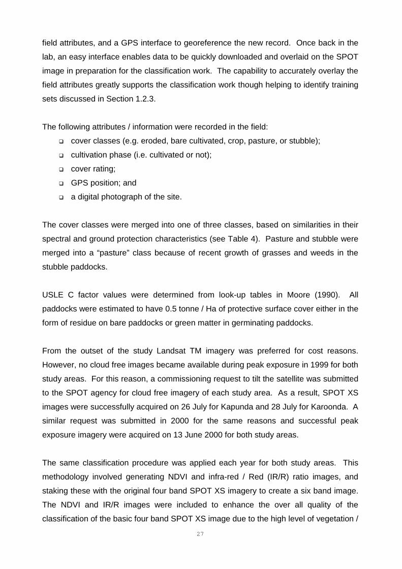
The image classification work was performed through a supervised image processing
classification technique using a “Maximum Likelihood” algorithm (ERDAS, 1999). The
classification procedure followed a two-phased approach, involving:
1. a stratification of the remaining agricultural areas into either bare, crop, or pasture
classes (see Table 3.), and then
2. once stratified, classifying each merged class area into the constituent cover class
values in Table 5.Table 5. Values for the USLE and WES C values.
C valuesCover type Mergedcover
classes
Description
USLE Cfactors
WES Cvalues
Eroded surface
Bare (recentlycultivated)
Bare No cover; unstable 0.5
3
Emergent crop;unstable
0.5 3
15 – 40 cm cropheight; moderateprotection
0.25 2
Crop Crop
> 40 cm crop height;well protected
0.175 0
Pasture < 40% soil cover; wellprotected
0.1 0
41 – 60% cover; stable 0.06 0
61 – 95% cover; stable 0.0065 0
Stubble withstabilising greenunderstorey
Pasture
> 95% cover; stable 0.0025 0
Following this, the classified areas were re-combined and re-coded according to their
respective USLE and WES values in preparation for the final GIS erosion susceptibility
model computation.
29
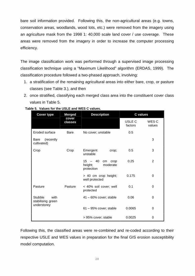
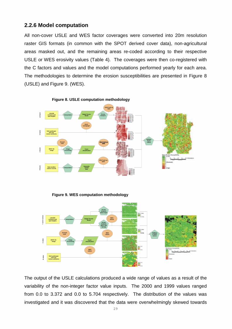
2.2.6 Model computation
All non-cover USLE and WES factor coverages were converted into 20m resolution
raster GIS formats (in common with the SPOT derived cover data), non-agricultural
areas masked out, and the remaining areas re-coded according to their respective
USLE or WES erosivity values (Table 4). The coverages were then co-registered with
the C factors and values and the model computations performed yearly for each area.
The methodologies to determine the erosion susceptibilities are presented in Figure 8
(USLE) and Figure 9. (WES).
Figure 8. USLE computation methodology
Figure 9. WES computation methodology
The output of the USLE calculations produced a wide range of values as a result of the
variability of the non-integer factor value inputs. The 2000 and 1999 values ranged
from 0.0 to 3.372 and 0.0 to 5.704 respectively. The distribution of the values was
investigated and it was discovered that the data were overwhelmingly skewed towards
InterpolationStatewide
rainfalldata
State weather station records
USLE look-uptable
Soil Landscape Unit soil
texture attributes
USLE nomograph
Terrain Analysis
1:50,000contours and spot heights
Interpolation Digital Terrain Model
USLE look-uptable
SPOT XS image
Ground truth
Image Processing
Cover classification
USLE look-uptable
USLE look-uptable
Multiply factor values
LS fa
ctor
K fa
ctor
C fa
ctor
R fa
ctor
Soil Landscape Unit soil
texture attributes
Terrain Analysis(NE & SW
facing)
1:50,000contours and spot heights
Interpolation Digital Terrain Model
SPOT XS image
Ground truth
Image Processing
Cover classification
WESvalues
Addition of WES values
C v
alue
E va
lue
Terrain Analysis
(dune tops)
WESvalues
WESvalues
30
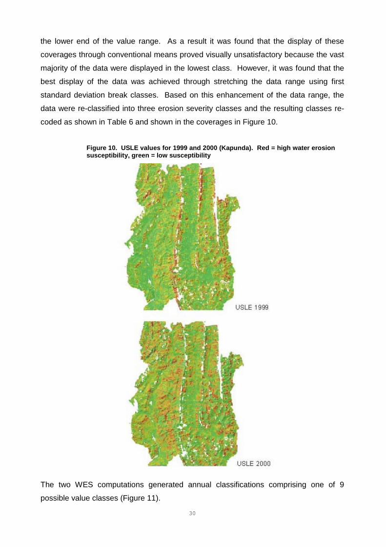
the lower end of the value range. As a result it was found that the display of these
coverages through conventional means proved visually unsatisfactory because the vast
majority of the data were displayed in the lowest class. However, it was found that the
best display of the data was achieved through stretching the data range using first
standard deviation break classes. Based on this enhancement of the data range, the
data were re-classified into three erosion severity classes and the resulting classes re-
coded as shown in Table 6 and shown in the coverages in Figure 10.
Figure 10. USLE values for 1999 and 2000 (Kapunda). Red = high water erosionsusceptibility, green = low susceptibility
The two WES computations generated annual classifications comprising one of 9
possible value classes (Figure 11).

31
Figure 11. WES values for 1999 and 2000 (Karoonda). Red = high wind erosionsusceptibility, green = low susceptibility
Table 6. The water erosion susceptibility classes based on USLE value ranges.
Water erosion risk class Re-class value USLE value range
Low risk 1 0.0 – 0.05
Moderate risk 2 0.05 – 0.24
High risk 3 0.24 – 5.704
The WES and USLE final coverages were investigated to determine the trends in the
intervening years. Firstly, a calculation of the percent of area covered by each risk
class was conducted for each year. Following this, a change detection was conducted
by subtracting the 1999 from the 2000 coverages, i.e. positive values indicating an
increase in erosion susceptibility in the period, and vice versa. The magnitudes of
32
changes were also identified through the procedure. The relative proportions in change
values were also investigated.
2.2.7 Results and conclusions
As discussed, the results of the soil erosion susceptibility modelling are presented in
Figure 10. and Figure 11. The images for each year were differenced using a GIS (year
2000 – year 1999) and the USLE results are shown in Figure 12 and WES in Figure 13.
A hill shade has been overlaid on these coverages to aid in the visual interpretation of
the information. It is evident from these coverages that the highest values coincide with
areas where there is poor ground protection covers and erosion prone landscape
variables. It is evident in the Kapunda study area the main “driver” of erosion
susceptibility is slope. This is borne by the fact that the erosion risk is greatest on the
steep ridges that run northwards through the study area and lowest in the low areas
between the ridges. In the Karoonda area however, the erosion susceptibility is strongly
governed by the presence of erodible soils that are predominantly located in the
southeast and northeast corner of the study area.
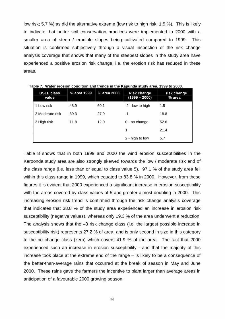
Table 7 shows the water erosion susceptibility trends for the Kapunda study area over
the two years. These data were generated from an analysis of the class distributions
from the resulting raster coverages. It is evident from a review of the data distribution in
Table 7 that the erosion susceptibilities of the study area are strongly skewed towards
the low erosion risk class in both years. In 2000 however, the area covered by the low
risk class experienced a significant increase (up by 11.1 %) at the expense of the
moderate risk areas (down by 11.4 %). The high erosion risk class area remains steady
in size during the two years. With the significant shift in favour of the low erosion risk
and the steady situation with the high-risk area, the net effect is that the erosion liability
for the Kapunda study area reduced in 2000 compared to the 1999 situation.
The risk change analysis reveals that over half of the study area experienced no overall
change in erosion susceptibility risk between the two years. Of the areas that did
experience a change, 27.1 % experienced a reduction (i.e. a positive change value),
whereas 21.3 % underwent an increase in erosion susceptibility (negative change
value). Four times the area experienced the largest possible positive shift (high risk to
33
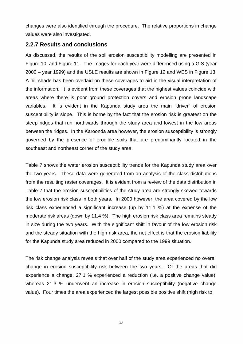
Figure 12. 2000 USLE minus 1999 USLE; red = an increased water erosionsusceptibility, green = reduction
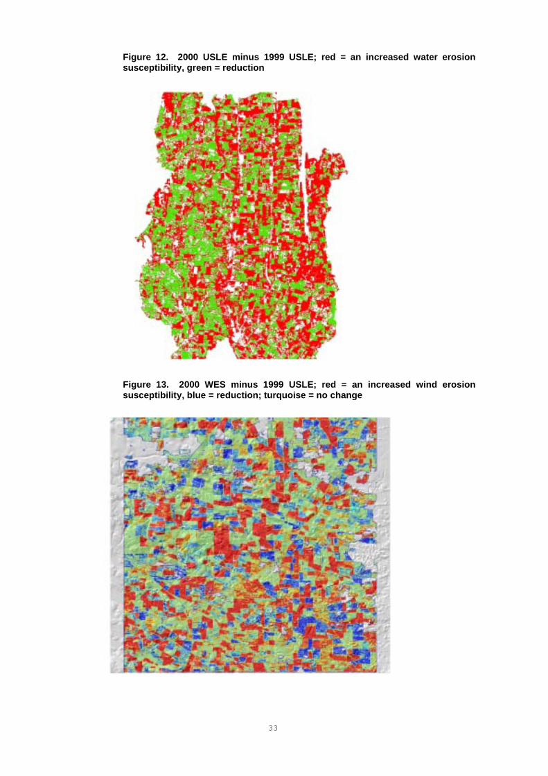
Figure 13. 2000 WES minus 1999 USLE; red = an increased wind erosionsusceptibility, blue = reduction; turquoise = no change
34
low risk; 5.7 %) as did the alternative extreme (low risk to high risk; 1.5 %). This is likely
to indicate that better soil conservation practices were implemented in 2000 with a
smaller area of steep / erodible slopes being cultivated compared to 1999. This
situation is confirmed subjectively through a visual inspection of the risk change
analysis coverage that shows that many of the steepest slopes in the study area have
experienced a positive erosion risk change, i.e. the erosion risk has reduced in these
areas.
Table 7. Water erosion condition and trends in the Kapunda study area, 1999 to 2000.
USLE classvalue
% area 1999 % area 2000 Risk change(1999 – 2000)
� risk change% area
1 Low risk 48.9 60.1 -2 - low to high 1.5
2 Moderate risk 39.3 27.9 -1 18.8
0 - no change 52.6
1 21.4
3 High risk 11.8 12.0
2 - high to low 5.7
Table 8 shows that in both 1999 and 2000 the wind erosion susceptibilities in the
Karoonda study area are also strongly skewed towards the low / moderate risk end of
the class range (i.e. less than or equal to class value 5). 97.1 % of the study area fell
within this class range in 1999, which equated to 83.8 % in 2000. However, from these
figures it is evident that 2000 experienced a significant increase in erosion susceptibility
with the areas covered by class values of 5 and greater almost doubling in 2000. This
increasing erosion risk trend is confirmed through the risk change analysis coverage
that indicates that 38.8 % of the study area experienced an increase in erosion risk
susceptibility (negative values), whereas only 19.3 % of the area underwent a reduction.
The analysis shows that the –3 risk change class (i.e. the largest possible increase in
susceptibility risk) represents 27.2 % of area, and is only second in size in this category
to the no change class (zero) which covers 41.9 % of the area. The fact that 2000
experienced such an increase in erosion susceptibility - and that the majority of this
increase took place at the extreme end of the range – is likely to be a consequence of
the better-than-average rains that occurred at the break of season in May and June
2000. These rains gave the farmers the incentive to plant larger than average areas in
anticipation of a favourable 2000 growing season.
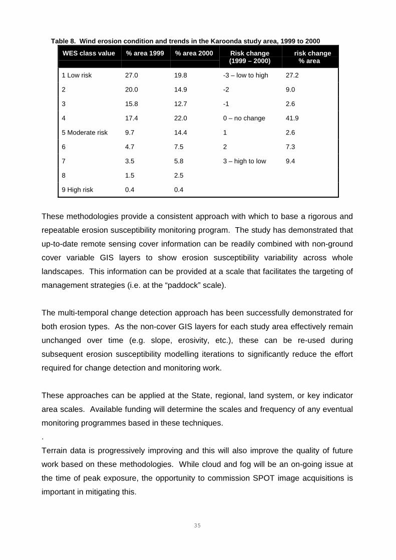
35
Table 8. Wind erosion condition and trends in the Karoonda study area, 1999 to 2000
WES class value % area 1999 % area 2000 Risk change(1999 – 2000)
� risk change% area
1 Low risk 27.0 19.8 -3 – low to high 27.2
2 20.0 14.9 -2 9.0
3 15.8 12.7 -1 2.6
4 17.4 22.0 0 – no change 41.9
5 Moderate risk 9.7 14.4 1 2.6
6 4.7 7.5 2 7.3
7 3.5 5.8 3 – high to low 9.4
8 1.5 2.5
9 High risk 0.4 0.4
These methodologies provide a consistent approach with which to base a rigorous and
repeatable erosion susceptibility monitoring program. The study has demonstrated that
up-to-date remote sensing cover information can be readily combined with non-ground
cover variable GIS layers to show erosion susceptibility variability across whole
landscapes. This information can be provided at a scale that facilitates the targeting of
management strategies (i.e. at the “paddock” scale).
The multi-temporal change detection approach has been successfully demonstrated for
both erosion types. As the non-cover GIS layers for each study area effectively remain
unchanged over time (e.g. slope, erosivity, etc.), these can be re-used during
subsequent erosion susceptibility modelling iterations to significantly reduce the effort
required for change detection and monitoring work.
These approaches can be applied at the State, regional, land system, or key indicator
area scales. Available funding will determine the scales and frequency of any eventual
monitoring programmes based in these techniques.
.
Terrain data is progressively improving and this will also improve the quality of future
work based on these methodologies. While cloud and fog will be an on-going issue at
the time of peak exposure, the opportunity to commission SPOT image acquisitions is
important in mitigating this.
36
The information provided by these approaches is valuable to land managers who wish
to locate areas in need of careful management on the property scale, or agricultural
policy makers who need to target initiatives and priorities on a regional scale.
Both models can be further refined - especially the WES - to ensure that the key
variables are used with the right weightings with regard to their ranked erosion
contributions.
The approach highlights the key benefit of using landscape variables in modelling
because the implications of poor protective ground covers are not the same in all areas.
For instance bare soils on steep slopes are far more susceptible to water erosion that in
flat areas.
2.3 Airborne remote sensing in cropping areas
The first airborne remote sensing survey conducted as part of the remote sensing study
was conducted over the Kapunda study area using the of Adelaide University’s airborne
remote sensing system. The set-up included:
� two Sony low resolution analogue video cameras (12 mm and 6 mm lens)
(VRS); and
� the Kodak DCS420c digital camera (ADP).
The two video cameras were flown to determine the relative merits of each lens setting
in VRS agricultural surveys.
The survey was conducted in December 1998 when much of the canola crop was wind
rowed and lying in the paddocks, the cereal crops mostly unharvested, and the grazing
paddocks were in various states of cover and having died back. The objectives of the
survey were to:
� gain familiarity with the University’s airborne remote sensing system – including
the SkyTrek in-flight navigation system;
� critically assess the quality of imagery, especially comparing the output of the
two VRS lenses;
� assess a roles for these systems in satellite remote sensing surrogate ground
truthing; and
� undertake a reconnaissance of the study area for familiarisation.
37
A flight altitude of approximately 400 m above ground was sought, although this proved
difficult to maintain at times over some areas due to the changing terrain and turbulence
that was encountered on the day. A route was planned to over fly a selection of the
variety of land systems within the study area, although an emphasis was given to the
area between Waterloo and Marrabel, located 40 and 20 Km to the north of Kapunda
respectively.
VRS recording was started as the Kapunda study area was entered and the recording
lasted for approximately 30 minutes. The video image recording was accompanied by a
voice recording of in flight comments made through a handheld microphone. The Horita
caption generator was in operation to record the GPS on the video frames throughout.
The ADP was triggered manually over areas of interest.
On completion of the flight the ADP imagery was downloaded and printed. Following
this, the equivalent areas covered by the 6 and 12 mm VRS were located from the video
tapes, framegrabbed and evaluated on-screen using the Adobe Photoshop graphics
software.
It was established that at approximately 400 m above ground the ADP resulted in a
resolution of approximately 10 cm on the ground. The ADP covered approximately 2/3
of the area on the ground of the 12 mm VRS, and had twice the resolution, i.e. 10 cm
whereas the 12 mm was 20 cm. The visual assessment confirmed that the 12 mm VRS
covered half the area of the 6 mm VRS, and had twice the resolution.
The visual inspection of the VRS revealed disappointing results with respect to the
visual quality of the imagery and was found lacking in tonal and colour variation. This
meant that the ground covers were insufficiently distinctive for successful API. The
problem was exacerbated over bright areas with low levels of soil cover. In contrast to
this, the ADP showed consistently high visual quality by achieving a combination of the
high resolution, colour and tonal variations. These differences in the quality of the VRS
and ADP systems are best illustrated through a visual comparison of the “frame 86”
triplicate shown in Figure 14. This frame was acquired over a farm yard, road and
cereal paddock. Reference to the ADP in this figure reveals excellent detail. This detail
is evident in the texture of the shed’s corrugated iron roof, the texture and colour of tree
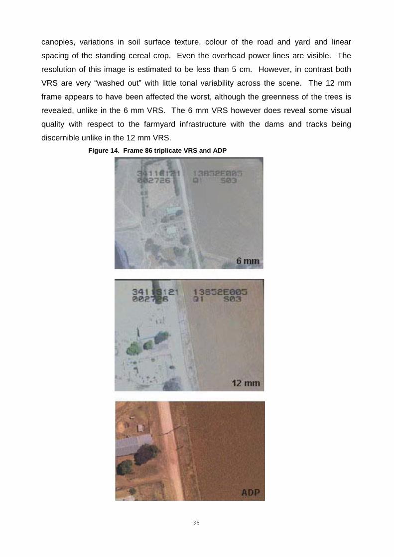
38
canopies, variations in soil surface texture, colour of the road and yard and linear
spacing of the standing cereal crop. Even the overhead power lines are visible. The
resolution of this image is estimated to be less than 5 cm. However, in contrast both
VRS are very “washed out” with little tonal variability across the scene. The 12 mm
frame appears to have been affected the worst, although the greenness of the trees is
revealed, unlike in the 6 mm VRS. The 6 mm VRS however does reveal some visual
quality with respect to the farmyard infrastructure with the dams and tracks being
discernible unlike in the 12 mm VRS.Figure 14. Frame 86 triplicate VRS and ADP
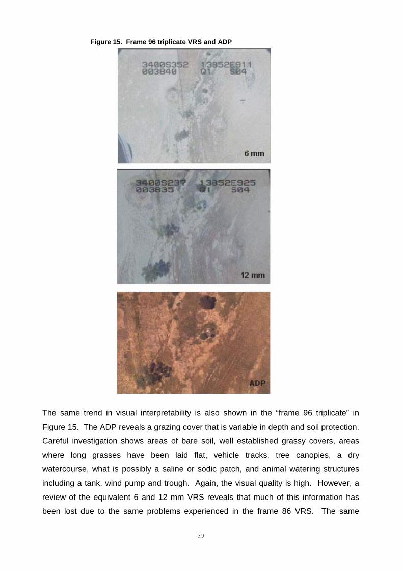
39
Figure 15. Frame 96 triplicate VRS and ADP
The same trend in visual interpretability is also shown in the “frame 96 triplicate” in
Figure 15. The ADP reveals a grazing cover that is variable in depth and soil protection.
Careful investigation shows areas of bare soil, well established grassy covers, areas
where long grasses have been laid flat, vehicle tracks, tree canopies, a dry
watercourse, what is possibly a saline or sodic patch, and animal watering structures
including a tank, wind pump and trough. Again, the visual quality is high. However, a
review of the equivalent 6 and 12 mm VRS reveals that much of this information has
been lost due to the same problems experienced in the frame 86 VRS. The same
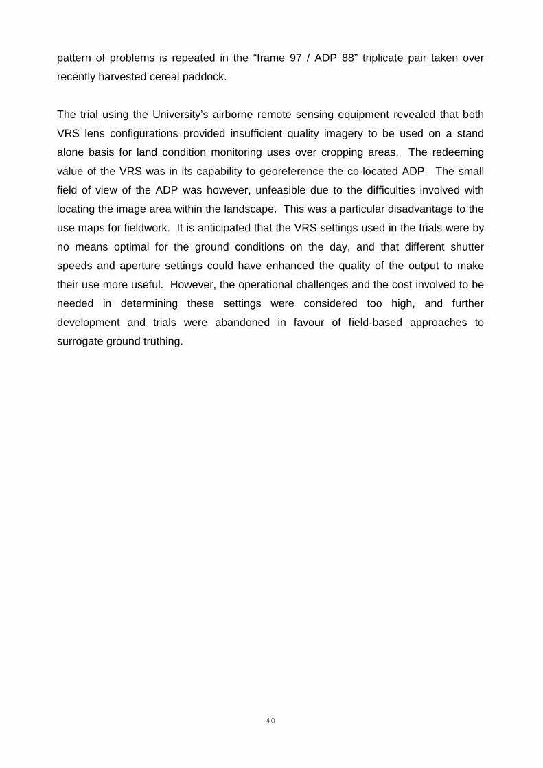
40
pattern of problems is repeated in the “frame 97 / ADP 88” triplicate pair taken over
recently harvested cereal paddock.
The trial using the University’s airborne remote sensing equipment revealed that both
VRS lens configurations provided insufficient quality imagery to be used on a stand
alone basis for land condition monitoring uses over cropping areas. The redeeming
value of the VRS was in its capability to georeference the co-located ADP. The small
field of view of the ADP was however, unfeasible due to the difficulties involved with
locating the image area within the landscape. This was a particular disadvantage to the
use maps for fieldwork. It is anticipated that the VRS settings used in the trials were by
no means optimal for the ground conditions on the day, and that different shutter
speeds and aperture settings could have enhanced the quality of the output to make
their use more useful. However, the operational challenges and the cost involved to be
needed in determining these settings were considered too high, and further
development and trials were abandoned in favour of field-based approaches to
surrogate ground truthing.
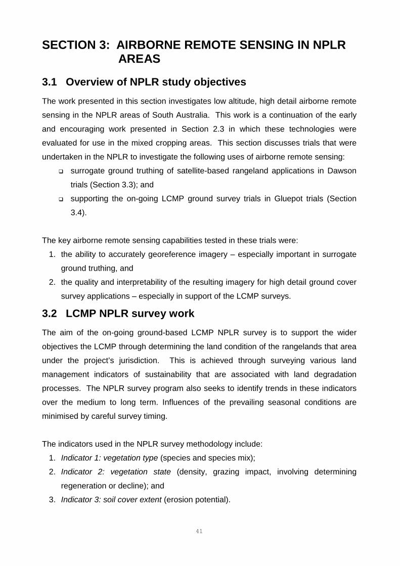
41
SECTION 3: AIRBORNE REMOTE SENSING IN NPLRAREAS
3.1 Overview of NPLR study objectivesThe work presented in this section investigates low altitude, high detail airborne remote
sensing in the NPLR areas of South Australia. This work is a continuation of the early
and encouraging work presented in Section 2.3 in which these technologies were
evaluated for use in the mixed cropping areas. This section discusses trials that were
undertaken in the NPLR to investigate the following uses of airborne remote sensing:
� surrogate ground truthing of satellite-based rangeland applications in Dawson
trials (Section 3.3); and
� supporting the on-going LCMP ground survey trials in Gluepot trials (Section
3.4).
The key airborne remote sensing capabilities tested in these trials were:
1. the ability to accurately georeference imagery – especially important in surrogate
ground truthing, and
2. the quality and interpretability of the resulting imagery for high detail ground cover
survey applications – especially in support of the LCMP surveys.
3.2 LCMP NPLR survey workThe aim of the on-going ground-based LCMP NPLR survey is to support the wider
objectives the LCMP through determining the land condition of the rangelands that area
under the project’s jurisdiction. This is achieved through surveying various land
management indicators of sustainability that are associated with land degradation
processes. The NPLR survey program also seeks to identify trends in these indicators
over the medium to long term. Influences of the prevailing seasonal conditions are
minimised by careful survey timing.
The indicators used in the NPLR survey methodology include:
1. Indicator 1: vegetation type (species and species mix);
2. Indicator 2: vegetation state (density, grazing impact, involving determining
regeneration or decline); and
3. Indicator 3: soil cover extent (erosion potential).
42
Like the LCMP surveys in the cropping areas, the NPLR surveys are conducted through
windscreen surveys along 2,500 Km of roads. The area that is surveyed covers
approximately 25,000 Km2 and is juxtaposed between the State’s cropping areas and
the pastoral lease areas. The primary land use of the area is extensive sheep grazing.
Unlike the cropping area LCMP windscreen surveys, the NPLR ones are performed at
fixed roadside locations, which are revisited on an annual basis. The annual survey
interval ensures that detailed trend information is collected, e.g. density changes and
species shifts. The roadside survey sites are currently numbered at 850. Each site has
been geo-referenced using GPS and photographed using a digital camera to provide a
visual reference during site location during subsequent re-visits. This information will
also enable change detection using fixed-point photography at a later date, if required at
a later date.
The surveys are conducted from the vehicle through a visual inspection within an
imagined 200 x 200 m area, 25 m off the side of the road. These surveys take place
during April in the period that usually coincides with the lowest levels of vegetation - and
therefore the highest erosion susceptibility. This is also the time when the perennial
plant composition is most prominent relative to the near-depleted annual plant
component, and is a key indicator of ecological resilience.
As with the LCMP in the cropping areas, the NPLR areas of the LCMP are divided into
monitoring zones. These zones are bound on the “outside” by the pastoral lease / non-
pastoral lease boundary and in the “inside” by the boundary of the land used for
cropping. These zones and the windscreen survey routes used are presented in Figure
1.
The windscreen surveys concentrate on rating the presence and condition of the
following vegetation types at each of the sites visited:
� Trees and shrubs: the three most dominant; grazing impact; and density.
� Low bushes (Chenopod and Chenopod-like bushes): the three most dominant;
grazing impact; density; and bush health.
� Native grasses: the three most dominant; grazing impact; and density.
� Annual plants: total surface cover, wet and dry; and forage value.
43
Given the experience developed in the airborne remote sensing systems through the
trials presented in Section 2.3 and in rangeland ecological monitoring work conducted
elsewhere (Thomas, 1998), the trials focussed on investigating airborne remote sensing
in determining the LCMP indicators which are presented above:
� Indicator 1: vegetation type (species and species mix) and
� Indicator 3: soil cover extent (erosion potential).
However, it was anticipated that the fine visual detail required to determine factors such
as grazing impact (e.g. observations of individual grass butts for grazing pressure)
under Indicator 2: vegetation state made it improbable that the airborne remote sensing
systems tested would be effective.
3.3 Dawson trials: surrogate ground truthingRemote sensing is an established methodology in rangeland monitoring. In Australian
rangelands, Landsat imagery have been shown to be highly effective in this work, e.g.
Pickup, Bastin and Chewings (1994); Bastin, Pickup and Stanes (1996); and Pickup,
Bastin and Chewings (1998). The key benefits of these satellite systems in this work
are that they are able to provide data that is suitable for application at the sub-regional
and landscape scales (30 m resolution), and that they are sensitive to the subtleties in
soil and plant spectral responses. Further, the often favourable, cloudless conditions
over these semi-arid areas ensures that images are rarely difficult to acquire.
One of the key requirements of successful satellite-based remote sensing is the need to
collect timely and accurate field data in preparation of the classification procedure as
discussed in Section 1.2.3. The process of collecting the field data needed to fulfil
these needs is labour intensive effort and is made harder due to the usual remoteness
of Australian rangelands.
With consideration for these issues, and the anticipation that satellite-based remote
sensing is likely to be effective in supporting the NPLR component of the LCMP at a
later date, an investigation of the role of airborne remote sensing was conducted.
3.3.1 The Dawson study area
An area located in the locality of Dawson within the West Yunta NPLR monitoring zone
was selected for this work. Figure 16 shows a Landsat TM image coverage of the area
that was acquired in May 1999. Five transects were located within the satellite image
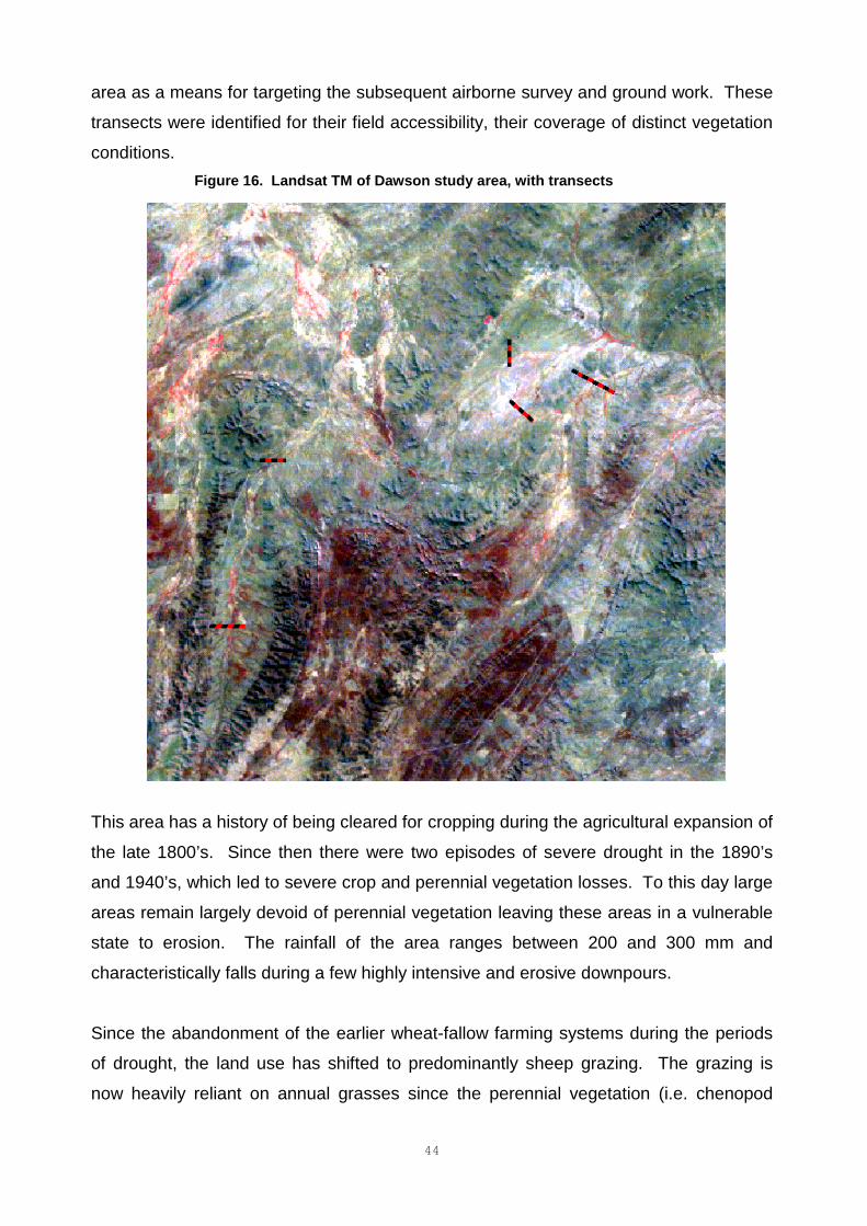
44
area as a means for targeting the subsequent airborne survey and ground work. These
transects were identified for their field accessibility, their coverage of distinct vegetation
conditions.Figure 16. Landsat TM of Dawson study area, with transects
This area has a history of being cleared for cropping during the agricultural expansion of
the late 1800’s. Since then there were two episodes of severe drought in the 1890’s
and 1940’s, which led to severe crop and perennial vegetation losses. To this day large
areas remain largely devoid of perennial vegetation leaving these areas in a vulnerable
state to erosion. The rainfall of the area ranges between 200 and 300 mm and
characteristically falls during a few highly intensive and erosive downpours.
Since the abandonment of the earlier wheat-fallow farming systems during the periods
of drought, the land use has shifted to predominantly sheep grazing. The grazing is
now heavily reliant on annual grasses since the perennial vegetation (i.e. chenopod
45
shrubs, annual forbs and grasses) in many of these areas are largely gone or are in
poor condition.
The soils of the area vary from shallow well-drained loams to shallow calcareous and
red duplex soils. The terrain ranges from low broad plains, gently sloping foot slopes
and steep hogback ridges (Butler and Dooley, 1990).
Typical plant species found in the area include: African boxthorn; pepper tree; Acacia
victoriea; red mallee; black bluebush; pearl bluebush; bladder saltbush; nitre bush;
annual saltbush; bindyi; onion weed and various annual and perennial grasses.
3.3.2 ADP survey and georegistration
The experience developed through the airborne trials in the Kapunda mixed cropping
areas (Section 2.3) indicated that the most the effective use of the technology in the
NPLR would involve using ADP, interpreted through API for various ground covers, with
VRS to provide georeferencing.
The airborne survey was conducted in October 1999 and used the configuration shown
in Figure 6, based on the following components:
� Cessna 172 aircraft;
� Sony 777P TV camera (28 mm lens) / Sony DSR-V10P digital video recorder
combination;
� Kodak DCS420c digital camera; and
� GPS equipment on-board.
The transects shown in Figure 20 were flown at approximately 1000 ft and 500 ft above
ground. The two heights were flown to evaluate the affect on the quality and usefulness
of the resulting images. The VRS system recorded continuously during the flight, whilst
the digital camera was triggered manually over the transects with the intention of
acquiring overlapping coverage of the transects. The start and end times for each
transect over-flight were recorded inside the aircraft. The GPS was set to acquire
position fixes at a rate of two per second. Flying conditions on the day were ideal with
no cloud cover and little turbulence. The flight was conducted in the middle of the day.
The following tasks were performed on the various datasets that were accumulated in
flight in preparation for subsequent field-based analysis:
� ADP download; ADP imagery were downloaded from the digital camera’s
PCMIA card and stored on a PC in TIFF format.
46
� VRS download; digital VRS over the five transects were located on the digital
video using the transect acquisition start / end times and were then
framegrabbed.
� VRS and ADP co-registration; framegrabbed VRS images were used to locate
the equivalent ADP coverage.
� GPS download; the GPS were downloaded from the unit and converted into an
ArcView GIS coverage of the flightline, and labelled with the acquisition
timecodes.
� Georegistration of ADP in the flightline GPS data; a link was established
between the ADP and VRS which ultimately provided the capability to
georeference the ADP using the GIS coverage of the GPS flightline. ArcView
was configured to enable the ADP frames to be inter-actively displayed over the
GIS coverages on screen by clicking on the GPS positions that had ADP links
using the software’s “hotlink” functionality. This proved to be a useful capability
in data presentation and in subsequent in fieldwork.
3.3.2.1 ADP quality assessment
An initial comparison of the ADP and VRS imagery confirmed the ADP to be
consistently better in terms of image quality. Of the ADP, it was found that the 500 ft
images yielded the best ground cover detail of the two survey altitudes, albeit at the
expense of area covered on the ground per frame and the extent of frame overlap which
was inconsistently achieved in the 1000 ft ADP. A decision was made to proceed with a
field-based assessment and verification of the 500 ft ADP only.
The 500 ft ADP frames that were available for the five transects were printed using a
high quality colour printer, georeferenced using the 500 ft VRS and these coordinates
up loaded to a handheld GPS in preparation of the field-based evaluation. The
evaluation process was subjectively based and concentrated on reviewing the utility of
500 ft ADP with particular emphasis on:
� ease of location of the ADP frame in the field, i.e. quality of georeferencing;
� soil and vegetation cover ratios; and if possible,
� the identification of plant species.
The fieldwork was conducted during February 2000. Localised rains had occurred in
the area shortly before the fieldwork, leading to the likelihood of cover inconsistencies
47
between the October airborne ground cover information and the February field
conditions.
The early stages of fieldwork revealed significant ADP georegistration problems:
1. None of the windscreen survey sites were successfully over flown due to
insufficiently accurate navigation during the over flights
2. Georeferencing errors in the ADP frames were discovered resulting in difficulty in
locating frames on the ground. These errors were sometimes as large as 500 m,
although most were within 300 m. However, it soon became apparent in the field
that the errors occurred along the flightline and were always located “up” the
flightline, i.e. in the direction the aircraft had come from. Therefore when
georeferencing errors were experienced, the search was progresses up the
flightline. The final confirmation that a frame had been successfully located was
achieved through matching up distinctive patterns found on the ground with those
shown in the frame, e.g. distinct groupings of pearl bluebush, a convergence of
sheep tracks, onion weed stands or a fallen tree. The ability to transpose a
pattern found in the field with those in the frames was initially poor – although
became easier with experience.
The source of the georeferencing errors can be explained through:
� the delays taken for the GPS unit to compute and transmit to the Horita the
position from the satellite signals;
� the time interval between the Horita receiving the GPS position signal and
converting it to a caption and transmitting it to the video recorder;
� aircraft roll and yaw, offsetting the GPS position from the (presumed) centre of
the frame; and
� positional errors through non-differentially corrected GPS.
The delays in GPS caption commitment to the frames can have a severe effect on the
georeferencing error of the ADP. For example, with an aircraft travelling at a ground
speed of 180 Km/h, a one second delay equates to an along track positional error of 50
m on the ground. An attempt was made to develop a system to systematically correct
for these errors by counting back along the GPS flightline positions in the GIS coverage
48
by a fixed interval, but this was abandoned because it was discovered that the errors
were non-systematic.
The ground resolution of the 500 ft ADP was estimated to be approximately 5 cm. This
resolution enabled a number of plant species to be classified with confidence,
particularly those with a canopy greater than 5 cm and non-ground hugging. It was
found that plants that threw a shadow greatly enhanced the classification process by
supplying information on form and structure. For example, red mallee was discernible
from other trees and bushes through their distinctive size and shape, and pepper trees
were distinguished though their verdant colour from other trees of the same size and
form. African boxthorn and acacia victoriea were difficult to distinguish from one
another. The chenopod shrubs were clearly visible but the species were not easy to
separate except for pearl bluebush which showed a very distinct grey-silver colour.
Nitre bush was distinguishable through their greenness and low-lying prostrate profile
that cast little shadow. Grasses and other smaller plants were not clearly
distinguishable, although clumps of onion weed were distinct through their characteristic
speckled effect in the imagery. Lichen bio-crusts were not distinguishable, with
confidence, from areas of bare soil, although bare eroded and scalded areas were
obvious from vegetated areas.
3.3.2.2 Operational considerations and discussion
As discussed, georeferencing errors of up to 500 m were experienced in the ADP and
these errors could not be systematically corrected. With errors of this size there could
be no assurance that an ADP frame would actually cover the corresponding location in
the satellite image. It was therefore considered that the ADP set-up used in these trials
was not be suitable for surrogate ground truthing. For example, a georeferencing error
of 300 m would equate to a positional error in a 30 m resolution Landsat image of up to
10 pixels. With positional errors such as these, the technology was considered
unacceptable in accurately locating training sets in the satellite imagery.
The abandonment of GPS selective has eliminated one of the important sources of
georegistration error. Further accuracies would be achieved though on-the-fly GPS
corrections through the integration of an inertia navigation system that corrects for
aircraft tip, roll and yaw as used in more the sophisticated commercially operated
airborne sensors. However, the introduction of this equipment would severely impact
on the flexibility and cost-effectiveness of the system.
49
The greatest enhancement to the over all georeferencing quality would be achieved
through ensuring a faster commitment of the GPS data onto the VRS frame through
enhancements to the Horita caption generator. Alternatively, the VRS system could be
by-passed in the georeferencing methodology through the use of the latest generation
of Kodak digital cameras that enables a direct link to be made from the GPS to the
camera, with the GPS data captioned inside the resulting ADP frame.
The key findings of the Dawson airborne remote sensing trials were that:
� the airborne systems tested were likely to prove unsuitable for satellite remote
sensing surrogate ground truthing due to the poor quality of georeferencing
achievable using the airborne remote sensing system described in this section,
and
� the quality ground cover information was shown to be good and seemed to offer
further opportunities for large scale, high detail rangeland monitoring
applications.
3.4 Gluepot trials: ground cover surveysThe Dawson study showed the quality of ground cover information from ADP frames to
be good and able to provide high quality ground cover information - similar in quality
and detail to the level of information from fieldwork. However, the quality of
georeferencing was revealed to be poor, making the technology difficult to use in
applications such as surrogate ground truthing that require good quality georeferencing
information.
“Frame sampling” is an airborne sampling technique that provides the opportunity of
conducting rapid, high quality ground surveys without the location biases often
associated with field-based surveys. The technique relies on good quality airborne
imagery without the need for precise georeferencing. Based on these requirements of
the sampling technique, a decision was made to continue with the evaluation of ADP to
identify a role for the technology in supporting of the objectives of the NPLR LCMP
through providing more effective, cost-effective rangeland cover sampling information.
Frame sampling involves collecting ADP at a regular interval along a flightline. Ideally
the flightline should be planned so that a well distributed coverage of the study area is
50
achieved, and is best accomplished by flying a grid or zigzag flightline. Back on the
ground, the ADP frames are downloaded and the ground covers from the frames
sampled through air photo interpretation to provide a cover rating for the whole
sampling area in the ADP frame.
The key benefits of ADP as an alternative to field-based sampling appear to lie in the
following key attributes:
� large study areas can be surveyed rapidly and systematically;
� the frames are photographic in quality and interpreted through well established
air photo interpretation;
� the reduction of fieldwork; and
� the surveying is conducted without bias, i.e. away from roadsides.
These qualities were assessed through trials in the “Gluepot” NPLR monitoring zone,
which is located to the east of Burra. The aim of the survey was to determine the
percentage coverage of vegetated versus non-vegetated covers as an important
indicator of rangeland condition and erosion susceptibility, and in the process,
determine the operational viability of the technique.
3.4.1 The Gluepot study area
The Gluepot study area is located east of Burra and is bound on the western side by the
flanks of the Southern Flinders and to the east by the pastoral lease areas (see Figure
17), and covers an area of approximately 3,950 Km2. Much of the study area receives
less than 250 mm of rainfall, and this falls mostly during the winter months and often
occurs sporadically and intensively.
The predominant land use of the area is extensive sheep grazing. The topography is
dominated by low rises with calcrete soils, intersected by plains and gentle slopes with
deep texture contrast soils derived predominantly from washout sediments. The
vegetation of the area is dominated by chenopod shrubs and grasses on the rises and
woody plants (e.g. casuarina and pepper corn trees) and grasses in the low lying areas.
Like the Dawson area, much of the area was cleared during the agricultural expansion
of the 1800’s but was abandoned during periods of prolonged drought. This clearance
has left the area denuded of much of the protective woody vegetation and in a degraded
state. In many places the poor land condition has been exacerbated by episodes of
rabbit plague and overstocking.
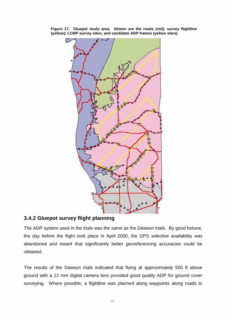
51
Figure 17. Gluepot study area. Shown are the roads (red); survey flightline(yellow); LCMP survey sites; and candidate ADP frames (yellow stars)
3.4.2 Gluepot survey flight planning
The ADP system used in the trials was the same as the Dawson trials. By good fortune,
the day before the flight took place in April 2000, the GPS selective availability was
abandoned and meant that significantly better georeferencing accuracies could be
obtained.
The results of the Dawson trials indicated that flying at approximately 500 ft above
ground with a 12 mm digital camera lens provided good quality ADP for ground cover
surveying. Where possible, a flightline was planned along waypoints along roads to
52
make easier access to sites during the subsequent fieldwork. In flight navigation was
supported by the SkyTrek system.
The automatic triggering device was set up to acquire one ADP frame every minute
during the flight, and the GPS was set to acquire once every four seconds.
The flight took over 2.5 hours, covered 480 Km, and produced 155 ADP frames (Figure
17). The flying conditions were ideal and the flight took place during the middle of the
day to reduce shadowing.
3.4.3 Frame sampling procedures
A procedure was developed to locate candidate ADP frames for the subsequent on-
ground investigations. This involved the following steps:
Step 1:– Downloading the ADP frames and the GPS record of the flightline;
Step 2:– Overlaying the GPS flightline with the road network using ArcView GIS to find
the portion of the flightline flown along the roads;
Step 3:– Recording the start and end times of the roadside portions from the GPS
coverage, and cross-referencing these with the VRS acquisition times;
Step 4:– Playing back the roadside portions of the VRS to visually match up the pictures
of the ground in the VRS with the equivalent ADP frames (36 ADP frames
identified in this way);
Step 5:– Georegistering the candidate ADP frames using the GPS positional data,
contained in the Horita captioning, directly off the VRS images; and finally
Step 6:– Plotting the positions of the candidate ADP frames along with the road network
to help plan the subsequent fieldwork.
The candidate ADP frames were printed on A4 sheets using a high quality printer before
the fieldwork. Their positions were also loaded into a GPS and used to locate the
candidate frames during the fieldwork.
3.4.3.1 ADP fieldwork
The 36 candidate ADP frames were visited one month after acquisition. The fieldwork
was conducted to:
� assess the georeferencing qualities of the ADP;
� conduct field orientation of the ADP fames by linking field conditions / features
with the ADP; and
53
� obtain field verification to assess quality of subsequent air photo interpretations.
Georeferencing qualities:- The positions of the candidate frames were loaded into a
GPS as waypoints to determine their field location. Although the GPS positions were
not affected by selective availability errors during the air survey, some difficulties were
nonetheless experienced in locating some of the frames. This was attributed to the lags
in committing and displaying the GPS points through the GPS / Horita combination. As
with the Dawson trials, when the location of candidate frames were not immediately
obvious in the field, a search along the flightline was conducted, and an error of
approximately 50 m was typically experienced. Six frames were located and surveyed
in this way within the limited time available in the field.
Field orientation and verification:- The frames that were successfully located in the field
were sampled for the following cover types, based on the structural classes used in the
NPLR windscreen surveys:
� woody plants;
� shrubs;
� herbaceous;
� grasses;
� litter (e.g. leaf and woody);
� bare soil;
� stones (gravels, stones, cobbles, etc.); and
� lichen bio-crusts.
The ground cover surveys were conducted by point-toe sampling. This method uses a
pin stuck into the toe of the surveyor’s boot to locate a sampling point on the ground
and involves pacing along a transect while counting each stride. At regular intervals of
strides the surveyor stops to identify the cover type found directly below the pin in the
boot. The cover type is then recorded on a field sheet. The Gluepot surveys involved
recording the ground covers at 100 survey points at an interval of every fifth stride. In
this way approximately 500 m were traversed within each frame using a fixed walking
pattern that ensured that all areas were covered.
As the ADP areas were being traversed during the sampling, the quality of the ground
cover information containing in the ADP was critically reviewed. It became apparent
54
that lichen, stones and bare soils were indistinguishable. In some cases it was also not
possible to distinguish accumulations of weathered, light woody litter. As was the case
in the Dawson trials, woody plants and shrubs were easily distinguished. Since the
acquisition of ADP, many of the perennial grasses had been browsed to their crowns
and could no longer be distinguished. Much of the annual grasses had been totally
removed. However, generally speaking it was possible to distinguish the plant covers
from the bare types of covers.
3.4.3.2 Frame sampling methodology
In the lab, a regular 10 x 10 grid of very fine crosses (100 points) was generated using
graphics software. These were then printed onto an A4 transparency that was overlaid
onto the high quality ADP prints (Figure 18). The fine crosses on the transparency were
used as sampling points for the ADP frames, which were then sampled through API. In
this process the cover types found directly under the sample points were recorded on
sheets and a percentage cover value for each cover type calculated from the 100
sample points. Shadows were sometimes found to cause problems with the
interpretation, particularly with chenopods that had dense, upright canopies. This,
however, was only an issue during the later stages of the flight when the sun angle was
lowest, and in these situations, a subjective decision was made as to whether the
shaded area was part of the canopy or not.
Of the 155 frames acquired during the flight, 66 were used in the frame sampling
exercise. The frames that were used included:
� the 6 frames that were surveyed in the field for use in verification;
� the remaining 30 candidate frames; and
� 30 additional frames that were selected from every third frame of those that
remained along the flightline to achieve a good geographic spread of the study
area.
As discussed, the field survey found that it was difficult to distinguish between the bare
types of covers, and so the frame sampling strategy was modified. The modified
sampling strategy involved sampling for areas that were covered (i.e. areas protected
from erosion) and areas that were bare and therefore susceptible to erosion. The bare
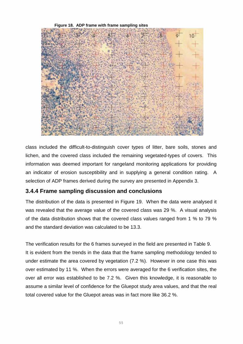
55
Figure 18. ADP frame with frame sampling sites
class included the difficult-to-distinguish cover types of litter, bare soils, stones and
lichen, and the covered class included the remaining vegetated-types of covers. This
information was deemed important for rangeland monitoring applications for providing
an indicator of erosion susceptibility and in supplying a general condition rating. A
selection of ADP frames derived during the survey are presented in Appendix 3.
3.4.4 Frame sampling discussion and conclusions
The distribution of the data is presented in Figure 19. When the data were analysed it
was revealed that the average value of the covered class was 29 %. A visual analysis
of the data distribution shows that the covered class values ranged from 1 % to 79 %
and the standard deviation was calculated to be 13.3.
The verification results for the 6 frames surveyed in the field are presented in Table 9.
It is evident from the trends in the data that the frame sampling methodology tended to
under estimate the area covered by vegetation (7.2 %). However in one case this was
over estimated by 11 %. When the errors were averaged for the 6 verification sites, the
over all error was established to be 7.2 %. Given this knowledge, it is reasonable to
assume a similar level of confidence for the Gluepot study area values, and that the real
total covered value for the Gluepot areas was in fact more like 36.2 %.
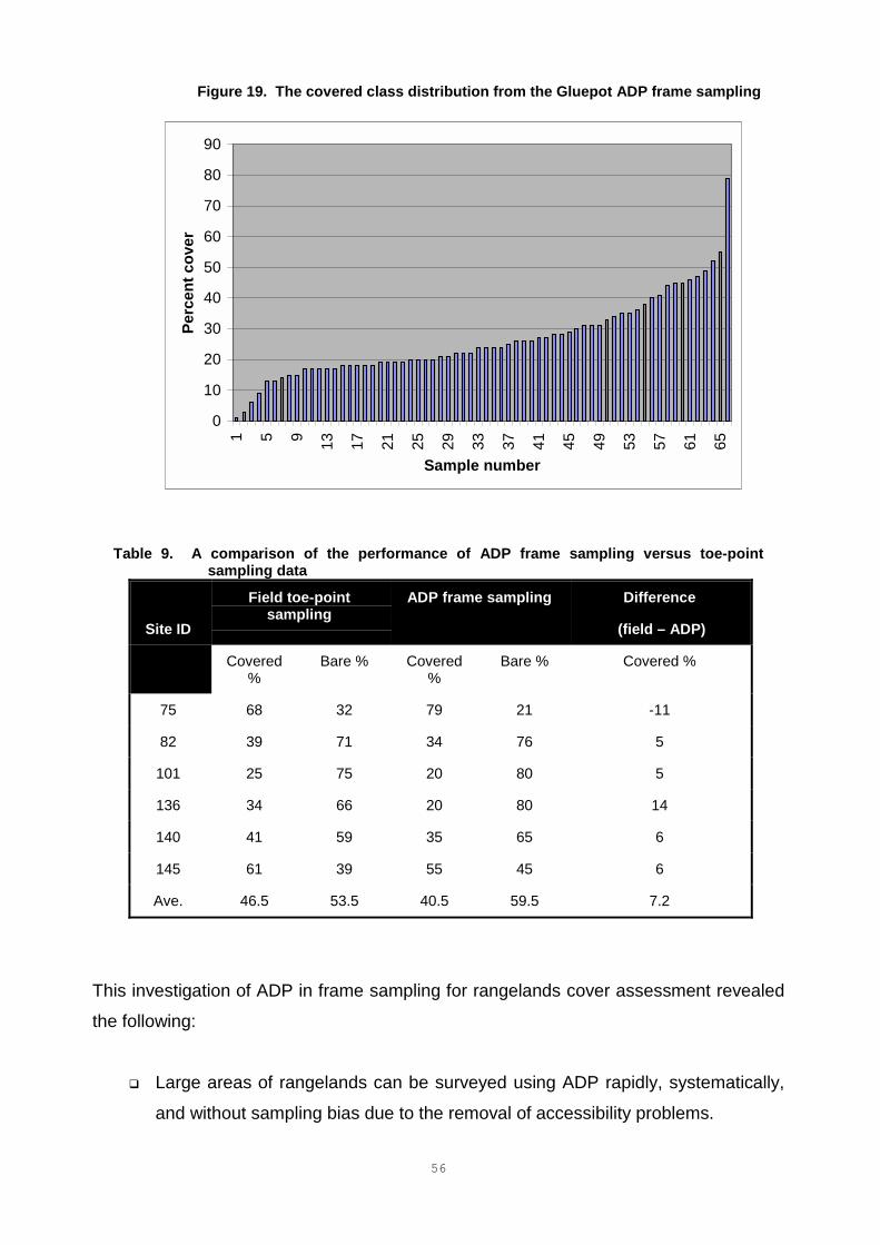
56
Figure 19. The covered class distribution from the Gluepot ADP frame sampling
Table 9. A comparison of the performance of ADP frame sampling versus toe-pointsampling data
Field toe-pointsampling
ADP frame sampling Difference
(field – ADP)Site ID
Covered%
Bare % Covered%
Bare % Covered %
75 68 32 79 21 -11
82 39 71 34 76 5
101 25 75 20 80 5
136 34 66 20 80 14
140 41 59 35 65 6
145 61 39 55 45 6
Ave. 46.5 53.5 40.5 59.5 7.2
This investigation of ADP in frame sampling for rangelands cover assessment revealed
the following:
� Large areas of rangelands can be surveyed using ADP rapidly, systematically,
and without sampling bias due to the removal of accessibility problems.
0
10
20
30
40
50
60
70
80
90
1 5 9 13 17 21 25 29 33 37 41 45 49 53 57 61 65
Sample number
Perc
ent c
over
57
� Although georeferencing problems still existed, these were not as great as
those encountered during the Dawson trials because of the removal of the GPS
selective availability.
� No significant difficulties were encountered during the field investigations in
distinguishing between covered classes (woody plants, shrubs, herbs and
grasses) from the printed ADP frames.
� However, difficulties were encountered in distinguishing between the bare
classes (litter, stones, bare soil and lichen), hence the decision to modify the
frame sampling classes into covered and bare classes during these trials.
� The frame sampling technique revealed the Gluepot study area to be 29 %
covered in vegetation.
� Based on the two-class scheme used, it was found that the sampling through air
photo interpretation under-estimated the amount of the covered class by 7.2 %.
58
SECTION 4: DRYLAND SALINITY REMOTE SENSING
4.1 Overview of dryland salinity objectivesThis section presents the work that was conducted to assess the role of remote sensing
and associated spatial modelling in mapping areas affected by dryland salinity as
assessing salinity risks. The approaches rely on the use of a number of remote sensing
approaches to derive degraded areas in the landscape, and use supporting
environmental and soils data to distinguish the saline affected areas from the degraded
areas.
4.2 Types of salinityIn common with much of Australia, South Australian soils are some of the most ancient
and highly weathered anywhere in the world. Their highly weathered condition often
contributes to a number of agricultural management issues associated with their
productive use. In particular, these issues contribute to:
� low fertility due to prolonged nutrient leaching / removal, as well as
� zones of elevated mineral ion salt concentrations within profiles.
These soils often experience constraints in their rooting zones to productive growth,
which has important implications to the water use efficiency of crops.
Salt in South Australian soils is predominantly derived predominantly from cyclic salt
(sea salt brought in by wind and rain) and also from the chemical weathering of soil
regolith materials. The most significant form of salinity in terms of economic impact in
the LCMP’s area is that of dryland salinity. Dryland salinity exists in primary (i.e.
naturally occurring) or secondary (i.e. man-made) forms. Secondary dryland salinity is
of particular concern to agriculture as it affects the largest area of land and is a problem
that continues to develop. Clarke (2000) revealed that the area affected by dryland
salinity in South Australia had increased from 55,000 Ha in 1988 to 400,000 Ha in 1993.
Dryland salinity is associated with the dual problems of waterlogging and the
development of high salt concentrations in the soil profile. It is caused by rising
watertables that occur as native vegetation is removed. Native vegetation clearance
began when European settlers took over land for agricultural purposes. The deeply
rooted native vegetation naturally regulated the watertable levels deep in the regolith
59
and soil profiles by utilising groundwater through transpiration. Removal of the
vegetation has allowed watertables to rise through the soil profile, carrying with it and
concentrating the naturally occurring salts. As the process continues, the watertables
reach the rooting zone of shallow rooted perennial crops and pastures, which become
affected by the dual problems of waterlogging and high salt concentrations. Under
these circumstances these crops may become non-viable to further reduce the overall
water use efficiency of the landscape. If the rise of the shallow watertable remains
unchecked, the water emerges at the surface in the low-lying parts of the landscape as
seepage areas. Seasonal changes in the watertable may cause these areas to dry out
resulting in scalds and salinas, or permanently inundated saline lakes and wetlands.
Severe impacts of dryland salinity occur downstream as aquifers and drainage systems
become contaminated with salinised irrigation and drinking water.
Another form of salinity that also exists in South Australia has been traditionally known
as dry saline land” although some researchers are now describing it as “transient
salinity” due to the transient nature of its expression. The complexity of the process of
this form of salinity is such that it defies clear understanding at the stage. Its process is
so difficult to analyse because the effects are difficult to isolate from other rooting zone
problems like sodicity, waterlogging and boron toxicity. However, it is known that dry
saline land salinity is not watertable related as is dryland salinity, and the salts are
mobilised up and down the soil profile by groundwater only in areas where the drainage
is impeded. This often occurs in very localised parts of the landscape and results in
quite discrete expressions. The problem is often largely ephemeral as the salts move in
and out of the rooting zone as seasonal water balance changes occur in the soil profile.
However, on some occasions the salts accumulate permanently on or near to the soil
surface as magnesic patches.
The ephemeral nature of dry saline land salinity and the current poor state of knowledge
of the processes means that this type of salinity is unlikely to be a suitable candidate for
remote sensing based assessment. On the other hand, dryland salinity is known to be
a growing problem. It is not transient, occurs over large areas and has indicators that
can be readily detected through remote sensing (e.g. waterlogging, surface
mineralisation and vegetation dieback). This combination of factors suggests that
60
conventional remote sensing is more likely to be successful in assessing it. The
following sections present the work conducted in these investigations.
4.3 Dryland salinity modelling rationale and approachThe extreme examples of salinity (i.e. salinas and seeps) form distinctive features within
the landscape. These cases of salinity are easily distinguished from surrounding
healthy vegetated areas using remote sensing through their distinctive spectra
comprising a combination of mineral, thermal and non-vegetated signatures.
Unfortunately, the spectra of erosion scars and salt pans are often confused as they are
both bare. Similarly, difficulties can also exist in distinguishing mild forms of salinity
from mild forms of erosion due to low levels of vegetation that often exist in these areas.
For these reasons the sole use of remote sensing for salinity work is likely to be
problematic, and is some cases, the best it will be able to do is discriminate between
degraded and good condition cover types. This problem was noted by Furby et al.
(1995 and 1997). These authors make the important point that expressions of dryland
salinity in the landscape are highly correlated to landscape factors such as terrain
location and soil type. This is because the formation of dryland salinity is caused by
rising watertables so that the first expressions often occur in the low-lying areas of the
landscape. In contrast to this, the authors also make the point that erosion is strongly
associated with slopes and higher up parts of the landscape, i.e. the parts of the
landscape least associated with dryland salinity.
The methodology developed in this study exploits this understanding of the role of
landscape in the development of dryland salinity. The methodology developed in this
study to map salinity is based on the following three stages:
Stage 1. Remote sensing was used to derive degraded areas in a landscape through
using remote sensing indicators related to soil wetness, vegetation condition and bare
areas.
Stage 2. Landscape information indicative of where salinity is likely to be expressed
within the landscape was combined with the degraded areas from the degraded areas
(mentioned above) to extract the saline areas through GIS-based spatial analysis. The
61
salinity contextual clues used were derived from various digital terrain models (DTMs)
and PIRSA’s soil land system mapping, e.g. waterlogging and erosion susceptibility,
depth to watertable, etc..
Stage 3. The areas deemed saline from the above were classified into the following
saline classes, i.e.:
� Saline risk areas, i.e. areas degraded due to permanent or perennial
waterlogging of saline groundwater, hosting stressed non-tolerant species
or tolerant species [e.g. sea barley grass (Hordeum marinum), salt water
couch (Paspalum vaginatum) or puccinellia];
� Severely saline areas, i.e. highly degraded areas that remain non-
vegetated or permanently host halophyte plant species [e.g. samphire
(Halosarcia pergranulata)].
The aim is that the methodology developed in this work will enable rapid and cost
effective classification of dryland salinity areas throughout a variety of land systems -
given access to suitable landscape process understanding and datasets.
The objectives of the study were therefore as follows:
1. Determine degradation spectral clues using operational remote sensing systems;
2. Derive salinity contextual clues from landscape datasets;
3. Combine the above through spatial modelling to extract out the saline risk areas
and severely saline areas from the degraded areas.
An important decision was made to conduct the analysis and modelling based on
datasets suitable for application at the 1: 50,000 scale. This scale was selected for its
ability to successfully represent the inherent spatial variability of the key features within
the landscape (e.g. landscape facets, slopes, soil properties, etc.) that govern the
salinisation process – and where it is ultimately expressed in the landscape.
Verification of results was done with the support of expert local knowledge of the land
systems, soils and landscape processes of the area (i.e. local land managers, PIRSA
staff, and the author’s acquired knowledge of the area). Additionally, information
derived from surrogate ground truthing from up-to-date air photographs and existing
salinity mapping played a vital role in the verification process.
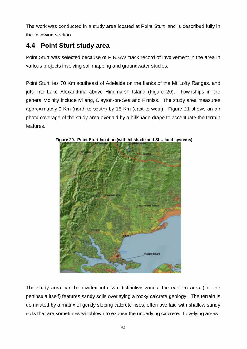
62
The work was conducted in a study area located at Point Sturt, and is described fully in
the following section.
4.4 Point Sturt study areaPoint Sturt was selected because of PIRSA’s track record of involvement in the area in
various projects involving soil mapping and groundwater studies.
Point Sturt lies 70 Km southeast of Adelaide on the flanks of the Mt Lofty Ranges, and
juts into Lake Alexandrina above Hindmarsh Island (Figure 20). Townships in the
general vicinity include Milang, Clayton-on-Sea and Finniss. The study area measures
approximately 9 Km (north to south) by 15 Km (east to west). Figure 21 shows an air
photo coverage of the study area overlaid by a hillshade drape to accentuate the terrain
features.
Figure 20. Point Sturt location (with hillshade and SLU land systems)
The study area can be divided into two distinctive zones: the eastern area (i.e. the
peninsula itself) features sandy soils overlaying a rocky calcrete geology. The terrain is
dominated by a matrix of gently sloping calcrete rises, often overlaid with shallow sandy
soils that are sometimes windblown to expose the underlying calcrete. Low-lying areas
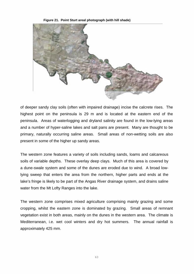
63
Figure 21. Point Sturt areal photograph (with hill shade)
of deeper sandy clay soils (often with impaired drainage) incise the calcrete rises. The
highest point on the peninsula is 29 m and is located at the eastern end of the
peninsula. Areas of waterlogging and dryland salinity are found in the low-lying areas
and a number of hyper-saline lakes and salt pans are present. Many are thought to be
primary, naturally occurring saline areas. Small areas of non-wetting soils are also
present in some of the higher up sandy areas.
The western zone features a variety of soils including sands, loams and calcareous
soils of variable depths. These overlay deep clays. Much of this area is covered by
a dune-swale system and some of the dunes are eroded due to wind. A broad low-
lying sweep that enters the area from the northern, higher parts and ends at the
lake’s fringe is likely to be part of the Angas River drainage system, and drains saline
water from the Mt Lofty Ranges into the lake.
The western zone comprises mixed agriculture comprising mainly grazing and some
cropping, whilst the eastern zone is dominated by grazing. Small areas of remnant
vegetation exist in both areas, mainly on the dunes in the western area. The climate is
Mediterranean, i.e. wet cool winters and dry hot summers. The annual rainfall is
approximately 425 mm.
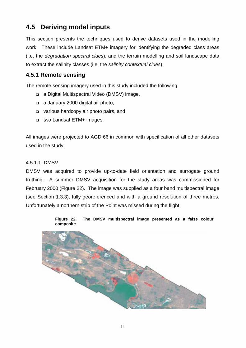
64
4.5 Deriving model inputsThis section presents the techniques used to derive datasets used in the modelling
work. These include Landsat ETM+ imagery for identifying the degraded class areas
(i.e. the degradation spectral clues), and the terrain modelling and soil landscape data
to extract the salinity classes (i.e. the salinity contextual clues).
4.5.1 Remote sensing
The remote sensing imagery used in this study included the following:
� a Digital Multispectral Video (DMSV) image,
� a January 2000 digital air photo,
� various hardcopy air photo pairs, and
� two Landsat ETM+ images.
All images were projected to AGD 66 in common with specification of all other datasets
used in the study.
4.5.1.1 DMSV
DMSV was acquired to provide up-to-date field orientation and surrogate ground
truthing. A summer DMSV acquisition for the study areas was commissioned for
February 2000 (Figure 22). The image was supplied as a four band multispectral image
(see Section 1.3.3), fully georeferenced and with a ground resolution of three metres.
Unfortunately a northern strip of the Point was missed during the flight.
Figure 22. The DMSV multispectral image presented as a false colourcomposite
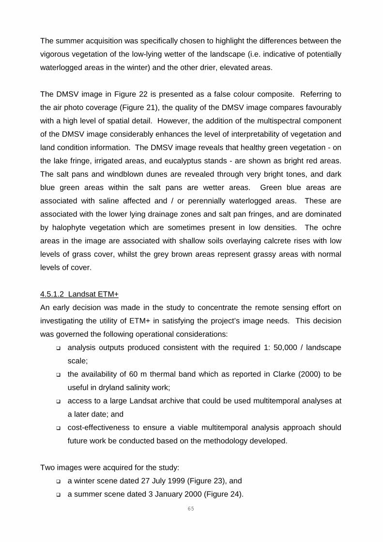
65
The summer acquisition was specifically chosen to highlight the differences between the
vigorous vegetation of the low-lying wetter of the landscape (i.e. indicative of potentially
waterlogged areas in the winter) and the other drier, elevated areas.
The DMSV image in Figure 22 is presented as a false colour composite. Referring to
the air photo coverage (Figure 21), the quality of the DMSV image compares favourably
with a high level of spatial detail. However, the addition of the multispectral component
of the DMSV image considerably enhances the level of interpretability of vegetation and
land condition information. The DMSV image reveals that healthy green vegetation - on
the lake fringe, irrigated areas, and eucalyptus stands - are shown as bright red areas.
The salt pans and windblown dunes are revealed through very bright tones, and dark
blue green areas within the salt pans are wetter areas. Green blue areas are
associated with saline affected and / or perennially waterlogged areas. These are
associated with the lower lying drainage zones and salt pan fringes, and are dominated
by halophyte vegetation which are sometimes present in low densities. The ochre
areas in the image are associated with shallow soils overlaying calcrete rises with low
levels of grass cover, whilst the grey brown areas represent grassy areas with normal
levels of cover.
4.5.1.2 Landsat ETM+
An early decision was made in the study to concentrate the remote sensing effort on
investigating the utility of ETM+ in satisfying the project’s image needs. This decision
was governed the following operational considerations:
� analysis outputs produced consistent with the required 1: 50,000 / landscape
scale;
� the availability of 60 m thermal band which as reported in Clarke (2000) to be
useful in dryland salinity work;
� access to a large Landsat archive that could be used multitemporal analyses at
a later date; and
� cost-effectiveness to ensure a viable multitemporal analysis approach should
future work be conducted based on the methodology developed.
Two images were acquired for the study:
� a winter scene dated 27 July 1999 (Figure 23), and
� a summer scene dated 3 January 2000 (Figure 24).
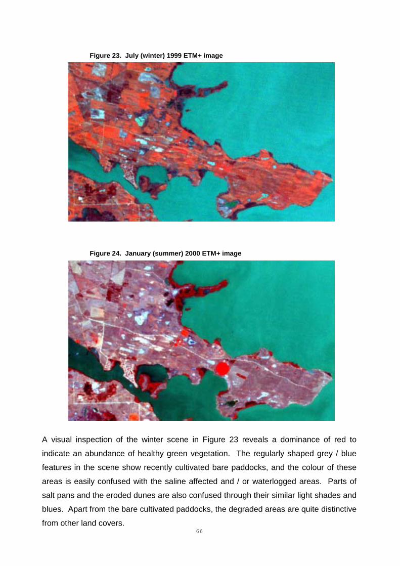
66
Figure 23. July (winter) 1999 ETM+ image
Figure 24. January (summer) 2000 ETM+ image
A visual inspection of the winter scene in Figure 23 reveals a dominance of red to
indicate an abundance of healthy green vegetation. The regularly shaped grey / blue
features in the scene show recently cultivated bare paddocks, and the colour of these
areas is easily confused with the saline affected and / or waterlogged areas. Parts of
salt pans and the eroded dunes are also confused through their similar light shades and
blues. Apart from the bare cultivated paddocks, the degraded areas are quite distinctive
from other land covers.
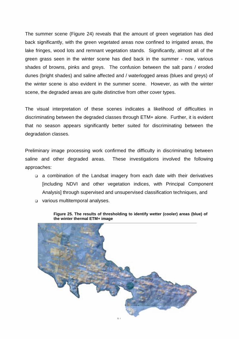
67
The summer scene (Figure 24) reveals that the amount of green vegetation has died
back significantly, with the green vegetated areas now confined to irrigated areas, the
lake fringes, wood lots and remnant vegetation stands. Significantly, almost all of the
green grass seen in the winter scene has died back in the summer - now, various
shades of browns, pinks and greys. The confusion between the salt pans / eroded
dunes (bright shades) and saline affected and / waterlogged areas (blues and greys) of
the winter scene is also evident in the summer scene. However, as with the winter
scene, the degraded areas are quite distinctive from other cover types.
The visual interpretation of these scenes indicates a likelihood of difficulties in
discriminating between the degraded classes through ETM+ alone. Further, it is evident
that no season appears significantly better suited for discriminating between the
degradation classes.
Preliminary image processing work confirmed the difficulty in discriminating between
saline and other degraded areas. These investigations involved the following
approaches:
� a combination of the Landsat imagery from each date with their derivatives
[including NDVI and other vegetation indices, with Principal Component
Analysis] through supervised and unsupervised classification techniques, and
� various multitemporal analyses.
Figure 25. The results of thresholding to identify wetter (cooler) areas (blue) ofthe winter thermal ETM+ image
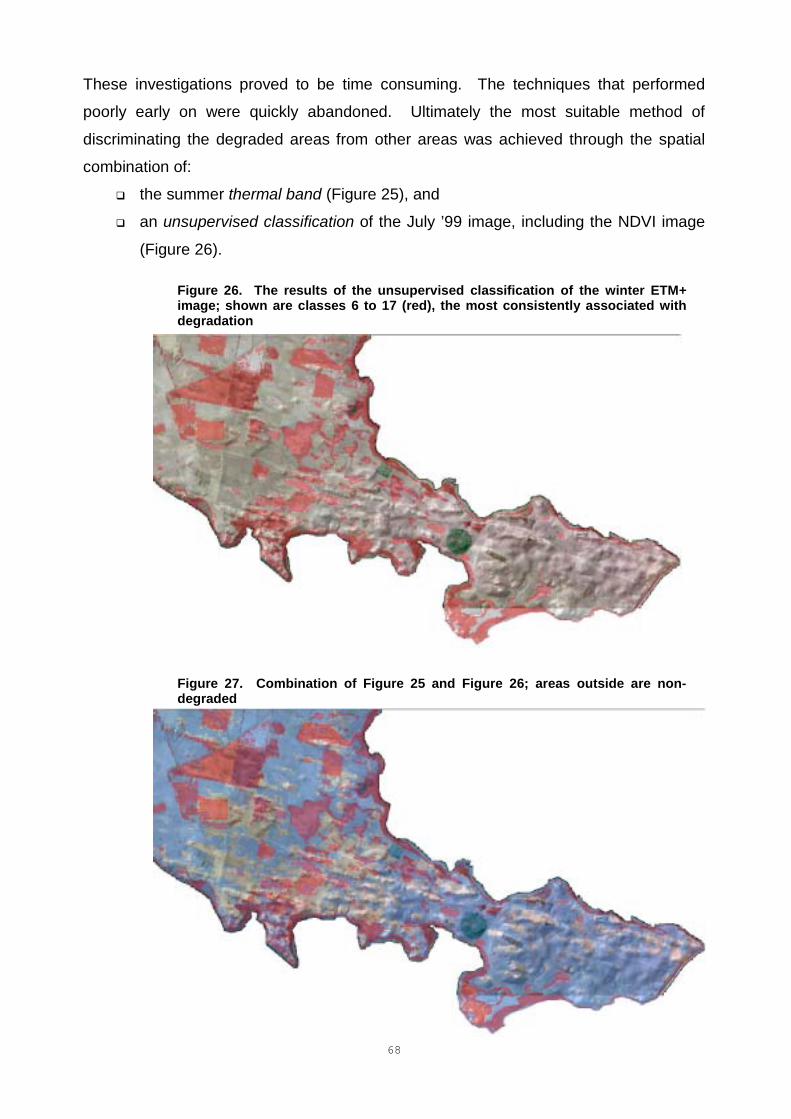
68
These investigations proved to be time consuming. The techniques that performed
poorly early on were quickly abandoned. Ultimately the most suitable method of
discriminating the degraded areas from other areas was achieved through the spatial
combination of:
� the summer thermal band (Figure 25), and
� an unsupervised classification of the July ’99 image, including the NDVI image
(Figure 26).
Figure 26. The results of the unsupervised classification of the winter ETM+image; shown are classes 6 to 17 (red), the most consistently associated withdegradation
Figure 27. Combination of Figure 25 and Figure 26; areas outside are non-degraded
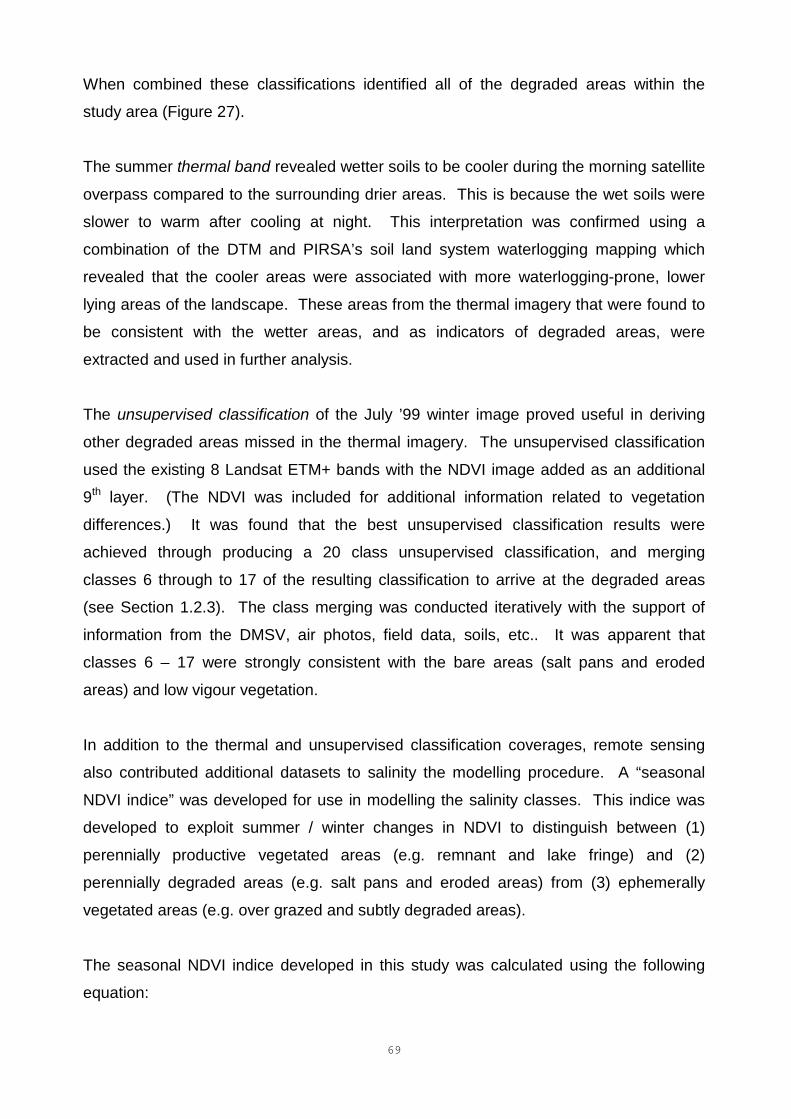
69
When combined these classifications identified all of the degraded areas within the
study area (Figure 27).
The summer thermal band revealed wetter soils to be cooler during the morning satellite
overpass compared to the surrounding drier areas. This is because the wet soils were
slower to warm after cooling at night. This interpretation was confirmed using a
combination of the DTM and PIRSA’s soil land system waterlogging mapping which
revealed that the cooler areas were associated with more waterlogging-prone, lower
lying areas of the landscape. These areas from the thermal imagery that were found to
be consistent with the wetter areas, and as indicators of degraded areas, were
extracted and used in further analysis.
The unsupervised classification of the July ’99 winter image proved useful in deriving
other degraded areas missed in the thermal imagery. The unsupervised classification
used the existing 8 Landsat ETM+ bands with the NDVI image added as an additional
9th layer. (The NDVI was included for additional information related to vegetation
differences.) It was found that the best unsupervised classification results were
achieved through producing a 20 class unsupervised classification, and merging
classes 6 through to 17 of the resulting classification to arrive at the degraded areas
(see Section 1.2.3). The class merging was conducted iteratively with the support of
information from the DMSV, air photos, field data, soils, etc.. It was apparent that
classes 6 – 17 were strongly consistent with the bare areas (salt pans and eroded
areas) and low vigour vegetation.
In addition to the thermal and unsupervised classification coverages, remote sensing
also contributed additional datasets to salinity the modelling procedure. A “seasonal
NDVI indice” was developed for use in modelling the salinity classes. This indice was
developed to exploit summer / winter changes in NDVI to distinguish between (1)
perennially productive vegetated areas (e.g. remnant and lake fringe) and (2)
perennially degraded areas (e.g. salt pans and eroded areas) from (3) ephemerally
vegetated areas (e.g. over grazed and subtly degraded areas).
The seasonal NDVI indice developed in this study was calculated using the following
equation:
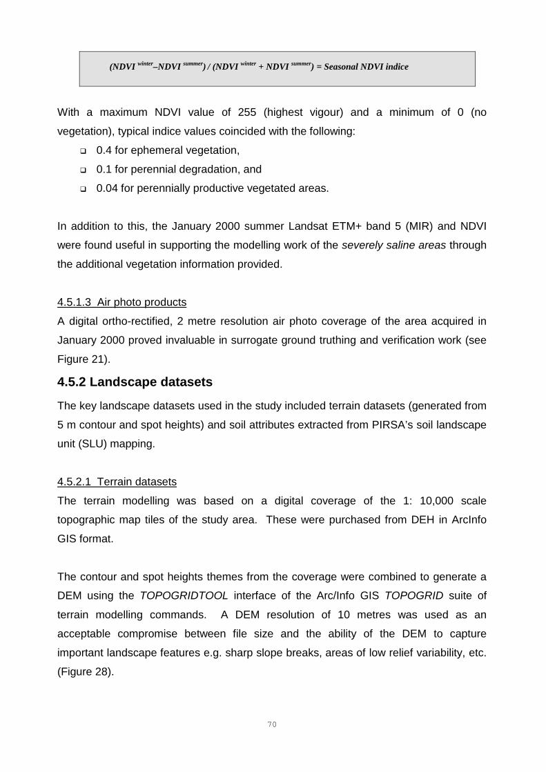
70
(NDVI winter–NDVI summer) / (NDVI winter + NDVI summer) = Seasonal NDVI indice
With a maximum NDVI value of 255 (highest vigour) and a minimum of 0 (no
vegetation), typical indice values coincided with the following:
� 0.4 for ephemeral vegetation,
� 0.1 for perennial degradation, and
� 0.04 for perennially productive vegetated areas.
In addition to this, the January 2000 summer Landsat ETM+ band 5 (MIR) and NDVI
were found useful in supporting the modelling work of the severely saline areas through
the additional vegetation information provided.
4.5.1.3 Air photo products
A digital ortho-rectified, 2 metre resolution air photo coverage of the area acquired in
January 2000 proved invaluable in surrogate ground truthing and verification work (see
Figure 21).
4.5.2 Landscape datasets
The key landscape datasets used in the study included terrain datasets (generated from
5 m contour and spot heights) and soil attributes extracted from PIRSA’s soil landscape
unit (SLU) mapping.
4.5.2.1 Terrain datasets
The terrain modelling was based on a digital coverage of the 1: 10,000 scale
topographic map tiles of the study area. These were purchased from DEH in ArcInfo
GIS format.
The contour and spot heights themes from the coverage were combined to generate a
DEM using the TOPOGRIDTOOL interface of the Arc/Info GIS TOPOGRID suite of
terrain modelling commands. A DEM resolution of 10 metres was used as an
acceptable compromise between file size and the ability of the DEM to capture
important landscape features e.g. sharp slope breaks, areas of low relief variability, etc.
(Figure 28).
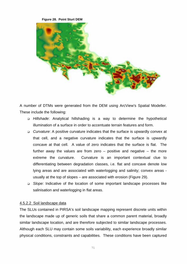
71
Figure 28. Point Sturt DEM
A number of DTMs were generated from the DEM using ArcView’s Spatial Modeller.
These include the following:
� Hillshade: Analytical hillshading is a way to determine the hypothetical
illumination of a surface in order to accentuate terrain features and form.
� Curvature: A positive curvature indicates that the surface is upwardly convex at
that cell, and a negative curvature indicates that the surface is upwardly
concave at that cell. A value of zero indicates that the surface is flat. The
further away the values are from zero – positive and negative – the more
extreme the curvature. Curvature is an important contextual clue to
differentiating between degradation classes, i.e. flat and concave denote low
lying areas and are associated with waterlogging and salinity; convex areas -
usually at the top of slopes – are associated with erosion (Figure 29).
� Slope: Indicative of the location of some important landscape processes like
salinisation and waterlogging in flat areas.
4.5.2.2 Soil landscape data
The SLUs contained in PIRSA’s soil landscape mapping represent discrete units within
the landscape made up of generic soils that share a common parent material, broadly
similar landscape location, and are therefore subjected to similar landscape processes.
Although each SLU may contain some soils variability, each experience broadly similar
physical conditions, constraints and capabilities. These conditions have been captured
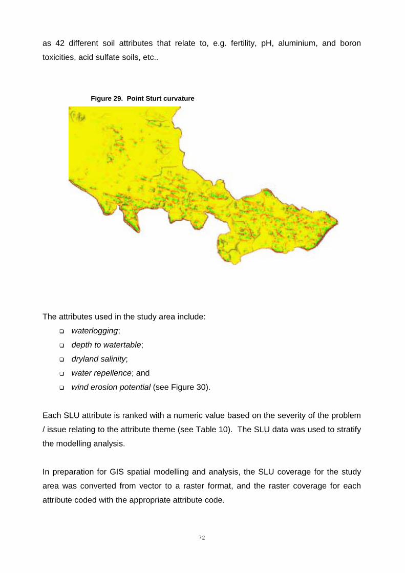
72
as 42 different soil attributes that relate to, e.g. fertility, pH, aluminium, and boron
toxicities, acid sulfate soils, etc..
Figure 29. Point Sturt curvature
The attributes used in the study area include:
� waterlogging;
� depth to watertable;
� dryland salinity;
� water repellence; and
� wind erosion potential (see Figure 30).
Each SLU attribute is ranked with a numeric value based on the severity of the problem
/ issue relating to the attribute theme (see Table 10). The SLU data was used to stratify
the modelling analysis.
In preparation for GIS spatial modelling and analysis, the SLU coverage for the study
area was converted from vector to a raster format, and the raster coverage for each
attribute coded with the appropriate attribute code.
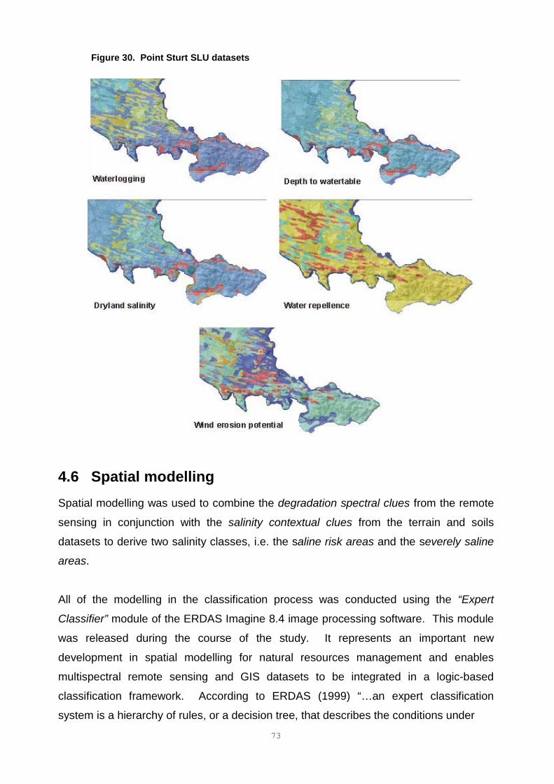
73
Figure 30. Point Sturt SLU datasets
4.6 Spatial modellingSpatial modelling was used to combine the degradation spectral clues from the remote
sensing in conjunction with the salinity contextual clues from the terrain and soils
datasets to derive two salinity classes, i.e. the saline risk areas and the severely saline
areas.
All of the modelling in the classification process was conducted using the “Expert
Classifier” module of the ERDAS Imagine 8.4 image processing software. This module
was released during the course of the study. It represents an important new
development in spatial modelling for natural resources management and enables
multispectral remote sensing and GIS datasets to be integrated in a logic-based
classification framework. According to ERDAS (1999) “…an expert classification
system is a hierarchy of rules, or a decision tree, that describes the conditions under
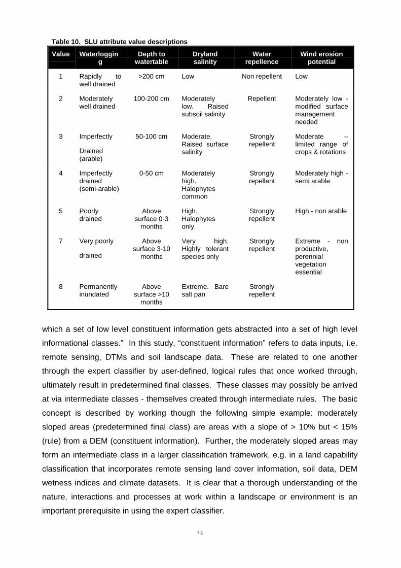
74
Table 10. SLU attribute value descriptions
Value Waterlogging
Depth towatertable
Drylandsalinity
Waterrepellence
Wind erosionpotential
1 Rapidly towell drained
>200 cm Low Non repellent Low
2 Moderatelywell drained
100-200 cm Moderatelylow. Raisedsubsoil salinity
Repellent Moderately low -modified surfacemanagementneeded
3 Imperfectly
Drained(arable)
50-100 cm Moderate.Raised surfacesalinity
Stronglyrepellent
Moderate –limited range ofcrops & rotations
4 Imperfectlydrained(semi-arable)
0-50 cm Moderatelyhigh.Halophytescommon
Stronglyrepellent
Moderately high -semi arable
5 Poorlydrained
Abovesurface 0-3
months
High.Halophytesonly
Stronglyrepellent
High - non arable
7 Very poorly
drained
Abovesurface 3-10
months
Very high.Highly tolerantspecies only
Stronglyrepellent
Extreme - nonproductive,perennialvegetationessential
8 Permanentlyinundated
Abovesurface >10
months
Extreme. Baresalt pan
Stronglyrepellent
which a set of low level constituent information gets abstracted into a set of high level
informational classes.” In this study, “constituent information” refers to data inputs, i.e.
remote sensing, DTMs and soil landscape data. These are related to one another
through the expert classifier by user-defined, logical rules that once worked through,
ultimately result in predetermined final classes. These classes may possibly be arrived
at via intermediate classes - themselves created through intermediate rules. The basic
concept is described by working though the following simple example: moderately
sloped areas (predetermined final class) are areas with a slope of > 10% but < 15%
(rule) from a DEM (constituent information). Further, the moderately sloped areas may
form an intermediate class in a larger classification framework, e.g. in a land capability
classification that incorporates remote sensing land cover information, soil data, DEM
wetness indices and climate datasets. It is clear that a thorough understanding of the
nature, interactions and processes at work within a landscape or environment is an
important prerequisite in using the expert classifier.
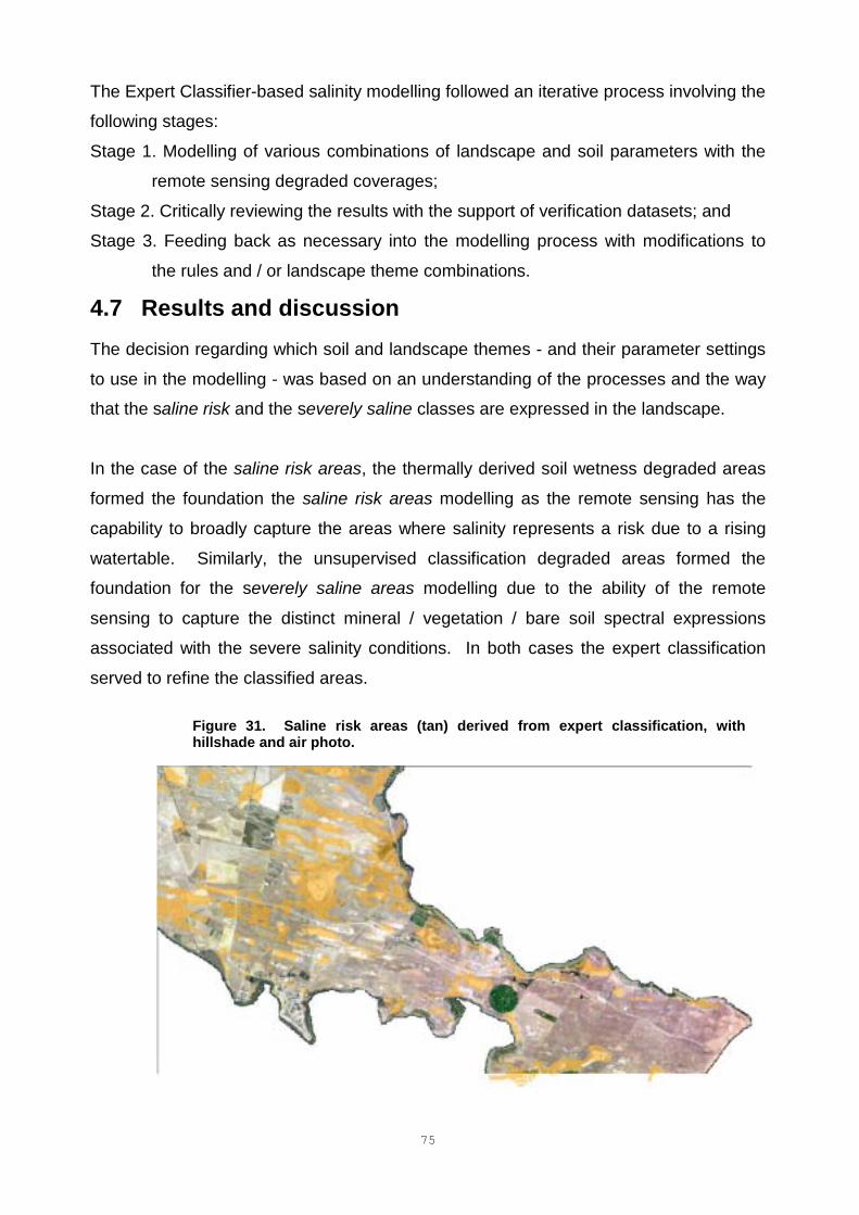
75
The Expert Classifier-based salinity modelling followed an iterative process involving the
following stages:
Stage 1. Modelling of various combinations of landscape and soil parameters with the
remote sensing degraded coverages;
Stage 2. Critically reviewing the results with the support of verification datasets; and
Stage 3. Feeding back as necessary into the modelling process with modifications to
the rules and / or landscape theme combinations.
4.7 Results and discussionThe decision regarding which soil and landscape themes - and their parameter settings
to use in the modelling - was based on an understanding of the processes and the way
that the saline risk and the severely saline classes are expressed in the landscape.
In the case of the saline risk areas, the thermally derived soil wetness degraded areas
formed the foundation the saline risk areas modelling as the remote sensing has the
capability to broadly capture the areas where salinity represents a risk due to a rising
watertable. Similarly, the unsupervised classification degraded areas formed the
foundation for the severely saline areas modelling due to the ability of the remote
sensing to capture the distinct mineral / vegetation / bare soil spectral expressions
associated with the severe salinity conditions. In both cases the expert classification
served to refine the classified areas.
Figure 31. Saline risk areas (tan) derived from expert classification, withhillshade and air photo.
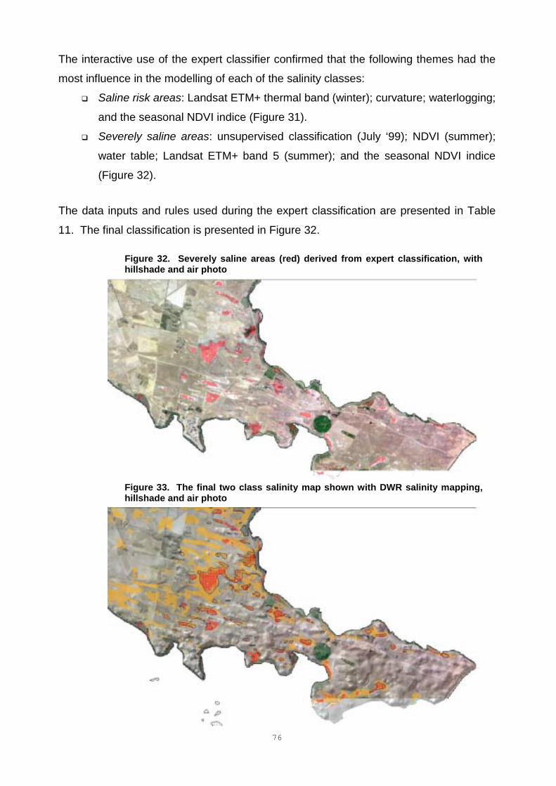
76
The interactive use of the expert classifier confirmed that the following themes had the
most influence in the modelling of each of the salinity classes:
� Saline risk areas: Landsat ETM+ thermal band (winter); curvature; waterlogging;
and the seasonal NDVI indice (Figure 31).
� Severely saline areas: unsupervised classification (July ‘99); NDVI (summer);
water table; Landsat ETM+ band 5 (summer); and the seasonal NDVI indice
(Figure 32).
The data inputs and rules used during the expert classification are presented in Table
11. The final classification is presented in Figure 32.
Figure 32. Severely saline areas (red) derived from expert classification, withhillshade and air photo
Figure 33. The final two class salinity map shown with DWR salinity mapping,hillshade and air photo
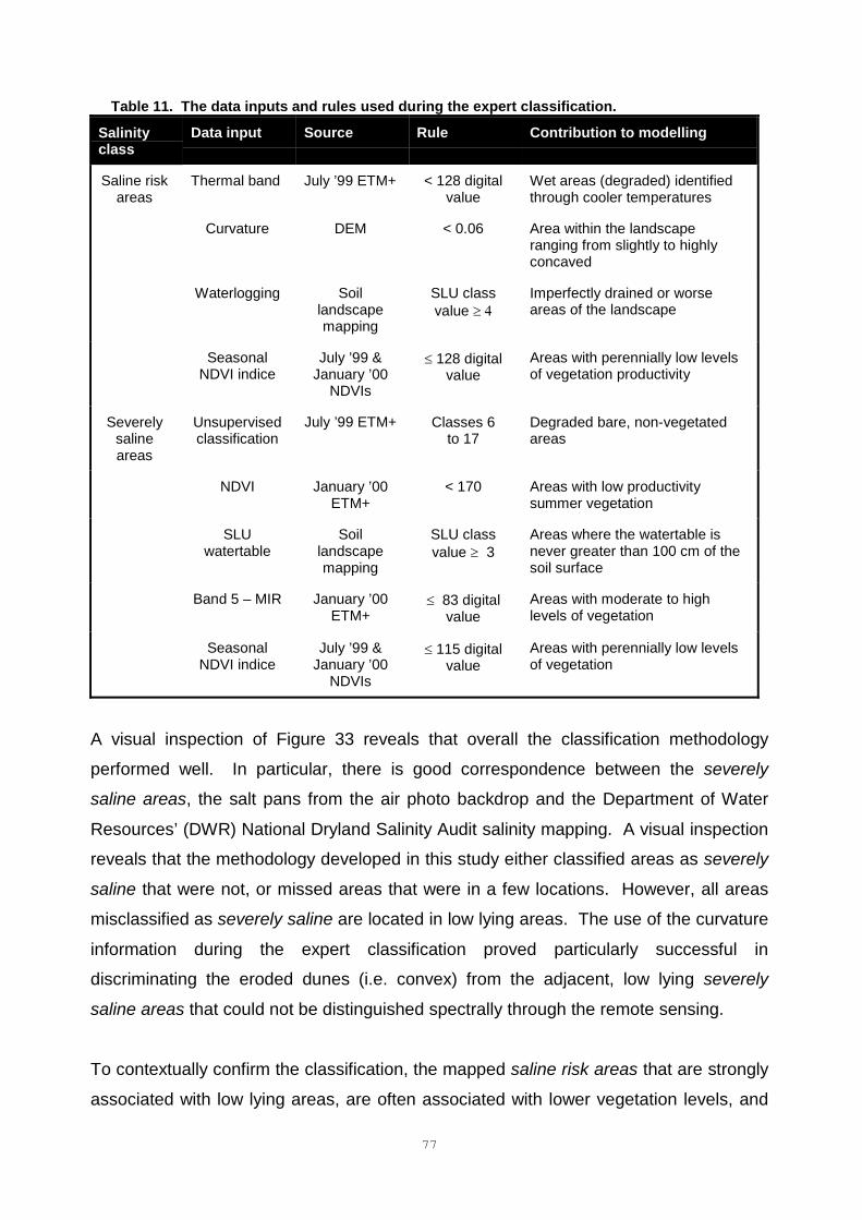
77
Table 11. The data inputs and rules used during the expert classification.
Salinityclass
Data input Source Rule Contribution to modelling
Saline riskareas
Thermal band July ’99 ETM+ < 128 digitalvalue
Wet areas (degraded) identifiedthrough cooler temperatures
Curvature DEM < 0.06 Area within the landscaperanging from slightly to highlyconcaved
Waterlogging Soillandscapemapping
SLU classvalue ���
Imperfectly drained or worseareas of the landscape
SeasonalNDVI indice
July ’99 &January ’00
NDVIs
� 128 digitalvalue
Areas with perennially low levelsof vegetation productivity
Severelysalineareas
Unsupervisedclassification
July ’99 ETM+ Classes 6to 17
Degraded bare, non-vegetatedareas
NDVI January ’00ETM+
< 170 Areas with low productivitysummer vegetation
SLUwatertable
Soillandscapemapping
SLU classvalue � 3
Areas where the watertable isnever greater than 100 cm of thesoil surface
Band 5 – MIR January ’00ETM+
� 83 digitalvalue
Areas with moderate to highlevels of vegetation
SeasonalNDVI indice
July ’99 &January ’00
NDVIs
� 115 digitalvalue
Areas with perennially low levelsof vegetation
A visual inspection of Figure 33 reveals that overall the classification methodology
performed well. In particular, there is good correspondence between the severely
saline areas, the salt pans from the air photo backdrop and the Department of Water
Resources’ (DWR) National Dryland Salinity Audit salinity mapping. A visual inspection
reveals that the methodology developed in this study either classified areas as severely
saline that were not, or missed areas that were in a few locations. However, all areas
misclassified as severely saline are located in low lying areas. The use of the curvature
information during the expert classification proved particularly successful in
discriminating the eroded dunes (i.e. convex) from the adjacent, low lying severely
saline areas that could not be distinguished spectrally through the remote sensing.
To contextually confirm the classification, the mapped saline risk areas that are strongly
associated with low lying areas, are often associated with lower vegetation levels, and
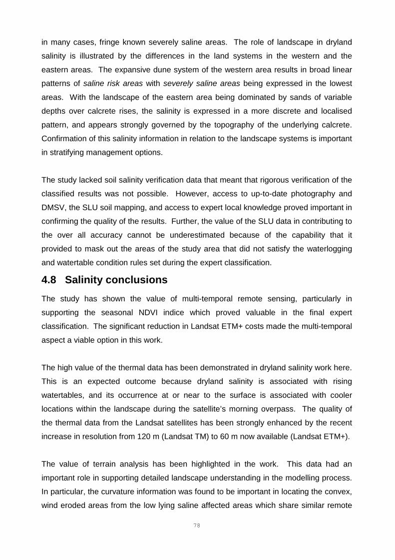
78
in many cases, fringe known severely saline areas. The role of landscape in dryland
salinity is illustrated by the differences in the land systems in the western and the
eastern areas. The expansive dune system of the western area results in broad linear
patterns of saline risk areas with severely saline areas being expressed in the lowest
areas. With the landscape of the eastern area being dominated by sands of variable
depths over calcrete rises, the salinity is expressed in a more discrete and localised
pattern, and appears strongly governed by the topography of the underlying calcrete.
Confirmation of this salinity information in relation to the landscape systems is important
in stratifying management options.
The study lacked soil salinity verification data that meant that rigorous verification of the
classified results was not possible. However, access to up-to-date photography and
DMSV, the SLU soil mapping, and access to expert local knowledge proved important in
confirming the quality of the results. Further, the value of the SLU data in contributing to
the over all accuracy cannot be underestimated because of the capability that it
provided to mask out the areas of the study area that did not satisfy the waterlogging
and watertable condition rules set during the expert classification.
4.8 Salinity conclusionsThe study has shown the value of multi-temporal remote sensing, particularly in
supporting the seasonal NDVI indice which proved valuable in the final expert
classification. The significant reduction in Landsat ETM+ costs made the multi-temporal
aspect a viable option in this work.
The high value of the thermal data has been demonstrated in dryland salinity work here.
This is an expected outcome because dryland salinity is associated with rising
watertables, and its occurrence at or near to the surface is associated with cooler
locations within the landscape during the satellite’s morning overpass. The quality of
the thermal data from the Landsat satellites has been strongly enhanced by the recent
increase in resolution from 120 m (Landsat TM) to 60 m now available (Landsat ETM+).
The value of terrain analysis has been highlighted in the work. This data had an
important role in supporting detailed landscape understanding in the modelling process.
In particular, the curvature information was found to be important in locating the convex,
wind eroded areas from the low lying saline affected areas which share similar remote

79
sensing spectra (bare soils). It should be noted that 5 m resolution contour data is only
available near to metropolitan areas in South Australia, and work outside these areas
will have to rely on less precise digital terrain models derived from the available 10 m
contour data. The operation implications of access to less precise terrain information
should be resolved for studies in these areas. However, it is likely that within a few
years high a resolution DEM will become available from NASA from a global RADAR
survey that was conducted in 1999, and routine access to this dataset is likely to greatly
increase the quality of terrain modelling data throughout all areas of rural Australia.
80
SECTION 5:
CONCLUSIONS AND RECOMMENDATIONS
5.1 OVER ALL CONCLUSIONSThis report has presented a number of trials involving the use of remote sensing with a
potential role in operational land condition monitoring in South Australia.
These technologies have been applied in determining peak erosion susceptibility in
mixed cropping areas prone to water erosion (Kapunda) and wind erosion (Karoonda).
The procedures have involved the combination landscape attributes with SPOT XS
satellite-derived land cover information within empirical erosion models through GIS-
based spatial modelling. The ability to monitor changes in annual peak erosion
susceptibilities in a consistent manner has been demonstrated. The resulting data are
suitable for application at the property / paddock scale.
The role of high resolution, georeferenced airborne remote sensing has been evaluated
in the NPLR areas in supporting potential applications in surrogate ground truthing of
satellite remote sensing and high detail cover sampling in these areas. The trials
demonstrated the difficulty for precisely georeferencing ADP in surrogate ground
truthing and it was concluded that unless georeferencing could be achieved within
approximately 30 m, the technique could not be operationally viable. However, given
the high visual quality of the ADP that could be produced, a large area, high detail
ground cover sampling technique was demonstrated that was not reliant on precise
georeferencing. It was concluded that this technique could be developed further to
become an operational detailed ground cover sampling tool in extensive grazing areas
such as the NPLR.
Finally, the report presents the outcomes of trials involving the use of remote sensing
systems in supporting dryland salinity risk mapping by combining various remote
sensing systems and landscape attributes through GIS spatial modelling. The
methodology demonstrated the importance of Landsat ETM+ derived information,
including thermal imagery to highlight waterlogged areas, and various vegetation and
mineral spectra to identify bare areas. These were able to derive “degraded areas”
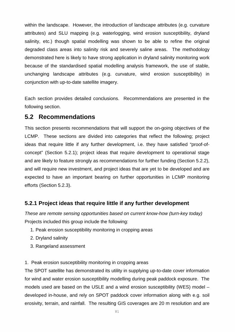
81
within the landscape. However, the introduction of landscape attributes (e.g. curvature
attributes) and SLU mapping (e.g. waterlogging, wind erosion susceptibility, dryland
salinity, etc.) though spatial modelling was shown to be able to refine the original
degraded class areas into salinity risk and severely saline areas. The methodology
demonstrated here is likely to have strong application in dryland salinity monitoring work
because of the standardised spatial modelling analysis framework, the use of stable,
unchanging landscape attributes (e.g. curvature, wind erosion susceptibility) in
conjunction with up-to-date satellite imagery.
Each section provides detailed conclusions. Recommendations are presented in the
following section.
5.2 RecommendationsThis section presents recommendations that will support the on-going objectives of the
LCMP. These sections are divided into categories that reflect the following; project
ideas that require little if any further development, i.e. they have satisfied “proof-of-
concept” (Section 5.2.1); project ideas that require development to operational stage
and are likely to feature strongly as recommendations for further funding (Section 5.2.2),
and will require new investment, and project ideas that are yet to be developed and are
expected to have an important bearing on further opportunities in LCMP monitoring
efforts (Section 5.2.3).
5.2.1 Project ideas that require little if any further development
These are remote sensing opportunities based on current know-how (turn-key today)
Projects included this group include the following:
1. Peak erosion susceptibility monitoring in cropping areas
2. Dryland salinity
3. Rangeland assessment
1. Peak erosion susceptibility monitoring in cropping areas
The SPOT satellite has demonstrated its utility in supplying up-to-date cover information
for wind and water erosion susceptibility modelling during peak paddock exposure. The
models used are based on the USLE and a wind erosion susceptibility (WES) model –
developed in-house, and rely on SPOT paddock cover information along with e.g. soil
erosivity, terrain, and rainfall. The resulting GIS coverages are 20 m resolution and are
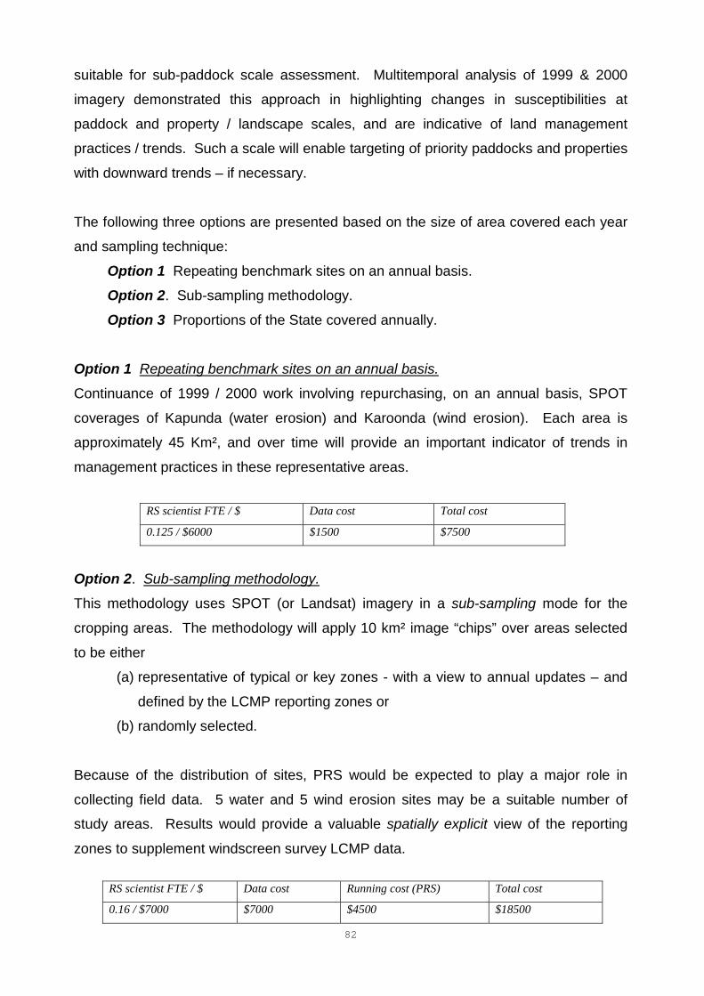
82
suitable for sub-paddock scale assessment. Multitemporal analysis of 1999 & 2000
imagery demonstrated this approach in highlighting changes in susceptibilities at
paddock and property / landscape scales, and are indicative of land management
practices / trends. Such a scale will enable targeting of priority paddocks and properties
with downward trends – if necessary.
The following three options are presented based on the size of area covered each year
and sampling technique:
Option 1 Repeating benchmark sites on an annual basis.
Option 2. Sub-sampling methodology.
Option 3 Proportions of the State covered annually.
Option 1 Repeating benchmark sites on an annual basis.
Continuance of 1999 / 2000 work involving repurchasing, on an annual basis, SPOT
coverages of Kapunda (water erosion) and Karoonda (wind erosion). Each area is
approximately 45 Km², and over time will provide an important indicator of trends in
management practices in these representative areas.
RS scientist FTE / $ Data cost Total cost
0.125 / $6000 $1500 $7500
Option 2. Sub-sampling methodology.
This methodology uses SPOT (or Landsat) imagery in a sub-sampling mode for the
cropping areas. The methodology will apply 10 km² image “chips” over areas selected
to be either
(a) representative of typical or key zones - with a view to annual updates – and
defined by the LCMP reporting zones or
(b) randomly selected.
Because of the distribution of sites, PRS would be expected to play a major role in
collecting field data. 5 water and 5 wind erosion sites may be a suitable number of
study areas. Results would provide a valuable spatially explicit view of the reporting
zones to supplement windscreen survey LCMP data.
RS scientist FTE / $ Data cost Running cost (PRS) Total cost
0.16 / $7000 $7000 $4500 $18500
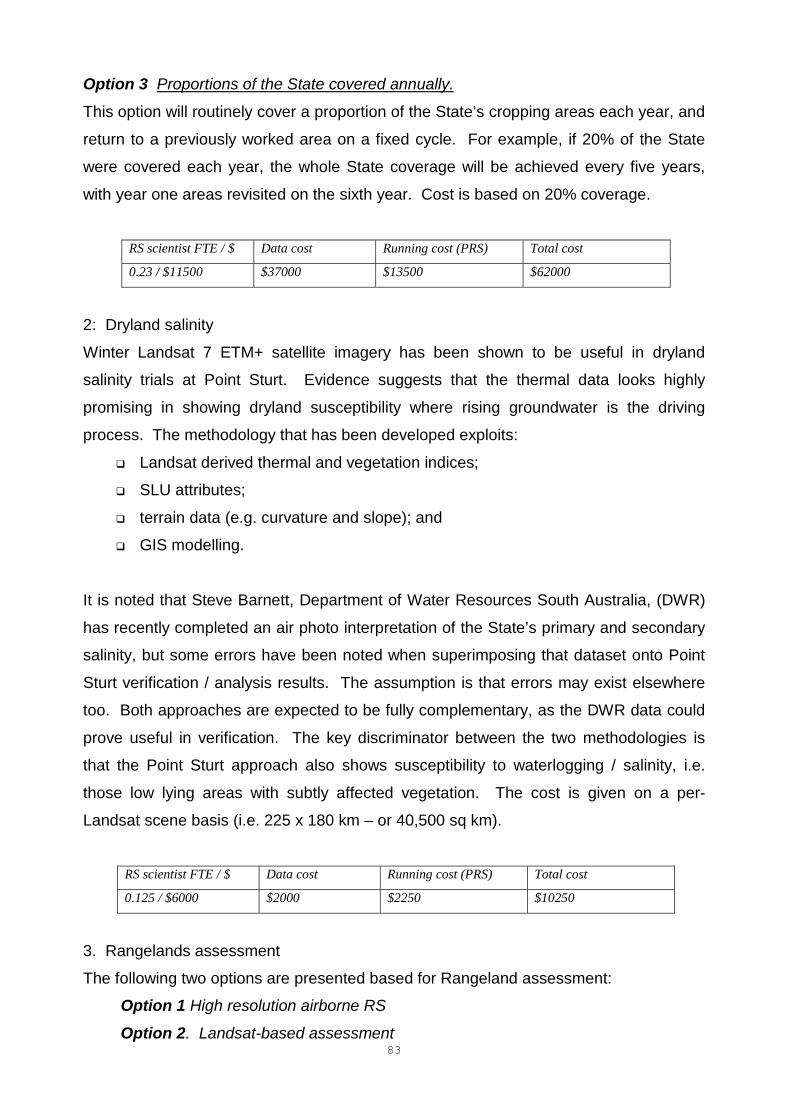
83
Option 3 Proportions of the State covered annually.
This option will routinely cover a proportion of the State’s cropping areas each year, and
return to a previously worked area on a fixed cycle. For example, if 20% of the State
were covered each year, the whole State coverage will be achieved every five years,
with year one areas revisited on the sixth year. Cost is based on 20% coverage.
RS scientist FTE / $ Data cost Running cost (PRS) Total cost
0.23 / $11500 $37000 $13500 $62000
2: Dryland salinity
Winter Landsat 7 ETM+ satellite imagery has been shown to be useful in dryland
salinity trials at Point Sturt. Evidence suggests that the thermal data looks highly
promising in showing dryland susceptibility where rising groundwater is the driving
process. The methodology that has been developed exploits:
� Landsat derived thermal and vegetation indices;
� SLU attributes;
� terrain data (e.g. curvature and slope); and
� GIS modelling.
It is noted that Steve Barnett, Department of Water Resources South Australia, (DWR)
has recently completed an air photo interpretation of the State’s primary and secondary
salinity, but some errors have been noted when superimposing that dataset onto Point
Sturt verification / analysis results. The assumption is that errors may exist elsewhere
too. Both approaches are expected to be fully complementary, as the DWR data could
prove useful in verification. The key discriminator between the two methodologies is
that the Point Sturt approach also shows susceptibility to waterlogging / salinity, i.e.
those low lying areas with subtly affected vegetation. The cost is given on a per-
Landsat scene basis (i.e. 225 x 180 km – or 40,500 sq km).
RS scientist FTE / $ Data cost Running cost (PRS) Total cost
0.125 / $6000 $2000 $2250 $10250
3. Rangelands assessment
The following two options are presented based for Rangeland assessment:
Option 1 High resolution airborne RS
Option 2. Landsat-based assessment
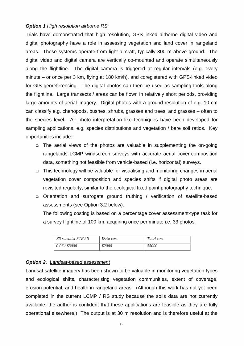
84
Option 1 High resolution airborne RS
Trials have demonstrated that high resolution, GPS-linked airborne digital video and
digital photography have a role in assessing vegetation and land cover in rangeland
areas. These systems operate from light aircraft, typically 300 m above ground. The
digital video and digital camera are vertically co-mounted and operate simultaneously
along the flightline. The digital camera is triggered at regular intervals (e.g. every
minute – or once per 3 km, flying at 180 km/h), and coregistered with GPS-linked video
for GIS georeferencing. The digital photos can then be used as sampling tools along
the flightline. Large transects / areas can be flown in relatively short periods, providing
large amounts of aerial imagery. Digital photos with a ground resolution of e.g. 10 cm
can classify e.g. chenopods, bushes, shrubs, grasses and trees; and grasses – often to
the species level. Air photo interpretation like techniques have been developed for
sampling applications, e.g. species distributions and vegetation / bare soil ratios. Key
opportunities include:
� The aerial views of the photos are valuable in supplementing the on-going
rangelands LCMP windscreen surveys with accurate aerial cover-composition
data, something not feasible from vehicle-based (i.e. horizontal) surveys.
� This technology will be valuable for visualising and monitoring changes in aerial
vegetation cover composition and species shifts if digital photo areas are
revisited regularly, similar to the ecological fixed point photography technique.
� Orientation and surrogate ground truthing / verification of satellite-based
assessments (see Option 3.2 below).
The following costing is based on a percentage cover assessment-type task for
a survey flightline of 100 km, acquiring once per minute i.e. 33 photos.
RS scientist FTE / $ Data cost Total cost
0.06 / $3000 $2000 $5000
Option 2. Landsat-based assessment
Landsat satellite imagery has been shown to be valuable in monitoring vegetation types
and ecological shifts, characterising vegetation communities, extent of coverage,
erosion potential, and health in rangeland areas. (Although this work has not yet been
completed in the current LCMP / RS study because the soils data are not currently
available, the author is confident that these applications are feasible as they are fully
operational elsewhere.) The output is at 30 m resolution and is therefore useful at the
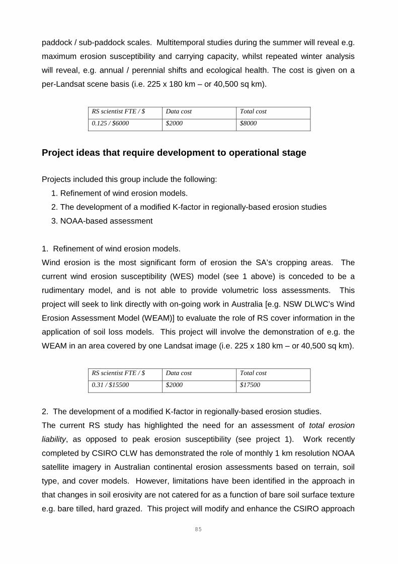
85
paddock / sub-paddock scales. Multitemporal studies during the summer will reveal e.g.
maximum erosion susceptibility and carrying capacity, whilst repeated winter analysis
will reveal, e.g. annual / perennial shifts and ecological health. The cost is given on a
per-Landsat scene basis (i.e. 225 x 180 km – or 40,500 sq km).
RS scientist FTE / $ Data cost Total cost
0.125 / $6000 $2000 $8000
Project ideas that require development to operational stage
Projects included this group include the following:
1. Refinement of wind erosion models.
2. The development of a modified K-factor in regionally-based erosion studies
3. NOAA-based assessment
1. Refinement of wind erosion models.
Wind erosion is the most significant form of erosion the SA’s cropping areas. The
current wind erosion susceptibility (WES) model (see 1 above) is conceded to be a
rudimentary model, and is not able to provide volumetric loss assessments. This
project will seek to link directly with on-going work in Australia [e.g. NSW DLWC’s Wind
Erosion Assessment Model (WEAM)] to evaluate the role of RS cover information in the
application of soil loss models. This project will involve the demonstration of e.g. the
WEAM in an area covered by one Landsat image (i.e. 225 x 180 km – or 40,500 sq km).
RS scientist FTE / $ Data cost Total cost
0.31 / $15500 $2000 $17500
2. The development of a modified K-factor in regionally-based erosion studies.
The current RS study has highlighted the need for an assessment of total erosion
liability, as opposed to peak erosion susceptibility (see project 1). Work recently
completed by CSIRO CLW has demonstrated the role of monthly 1 km resolution NOAA
satellite imagery in Australian continental erosion assessments based on terrain, soil
type, and cover models. However, limitations have been identified in the approach in
that changes in soil erosivity are not catered for as a function of bare soil surface texture
e.g. bare tilled, hard grazed. This project will modify and enhance the CSIRO approach
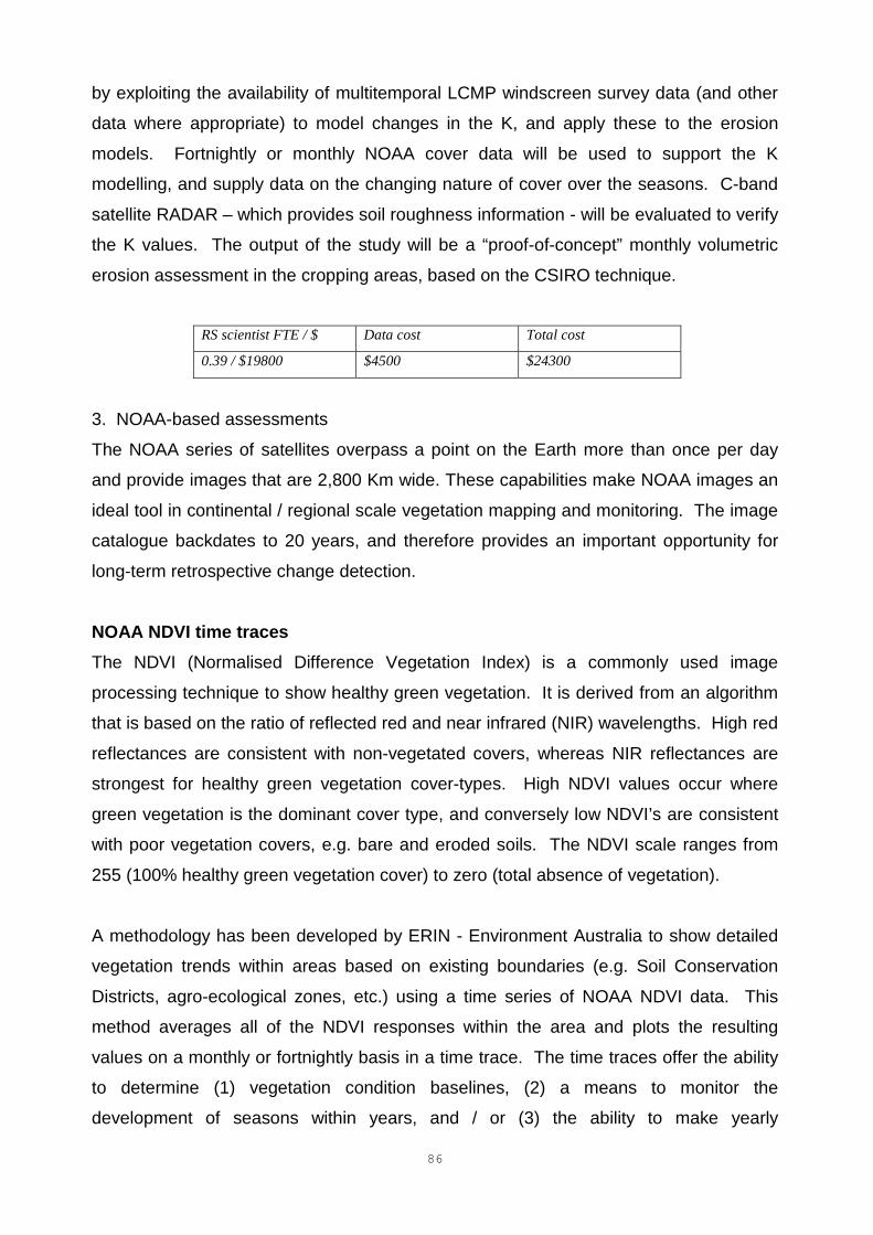
86
by exploiting the availability of multitemporal LCMP windscreen survey data (and other
data where appropriate) to model changes in the K, and apply these to the erosion
models. Fortnightly or monthly NOAA cover data will be used to support the K
modelling, and supply data on the changing nature of cover over the seasons. C-band
satellite RADAR – which provides soil roughness information - will be evaluated to verify
the K values. The output of the study will be a “proof-of-concept” monthly volumetric
erosion assessment in the cropping areas, based on the CSIRO technique.
RS scientist FTE / $ Data cost Total cost
0.39 / $19800 $4500 $24300
3. NOAA-based assessments
The NOAA series of satellites overpass a point on the Earth more than once per day
and provide images that are 2,800 Km wide. These capabilities make NOAA images an
ideal tool in continental / regional scale vegetation mapping and monitoring. The image
catalogue backdates to 20 years, and therefore provides an important opportunity for
long-term retrospective change detection.
NOAA NDVI time tracesThe NDVI (Normalised Difference Vegetation Index) is a commonly used image
processing technique to show healthy green vegetation. It is derived from an algorithm
that is based on the ratio of reflected red and near infrared (NIR) wavelengths. High red
reflectances are consistent with non-vegetated covers, whereas NIR reflectances are
strongest for healthy green vegetation cover-types. High NDVI values occur where
green vegetation is the dominant cover type, and conversely low NDVI’s are consistent
with poor vegetation covers, e.g. bare and eroded soils. The NDVI scale ranges from
255 (100% healthy green vegetation cover) to zero (total absence of vegetation).
A methodology has been developed by ERIN - Environment Australia to show detailed
vegetation trends within areas based on existing boundaries (e.g. Soil Conservation
Districts, agro-ecological zones, etc.) using a time series of NOAA NDVI data. This
method averages all of the NDVI responses within the area and plots the resulting
values on a monthly or fortnightly basis in a time trace. The time traces offer the ability
to determine (1) vegetation condition baselines, (2) a means to monitor the
development of seasons within years, and / or (3) the ability to make yearly
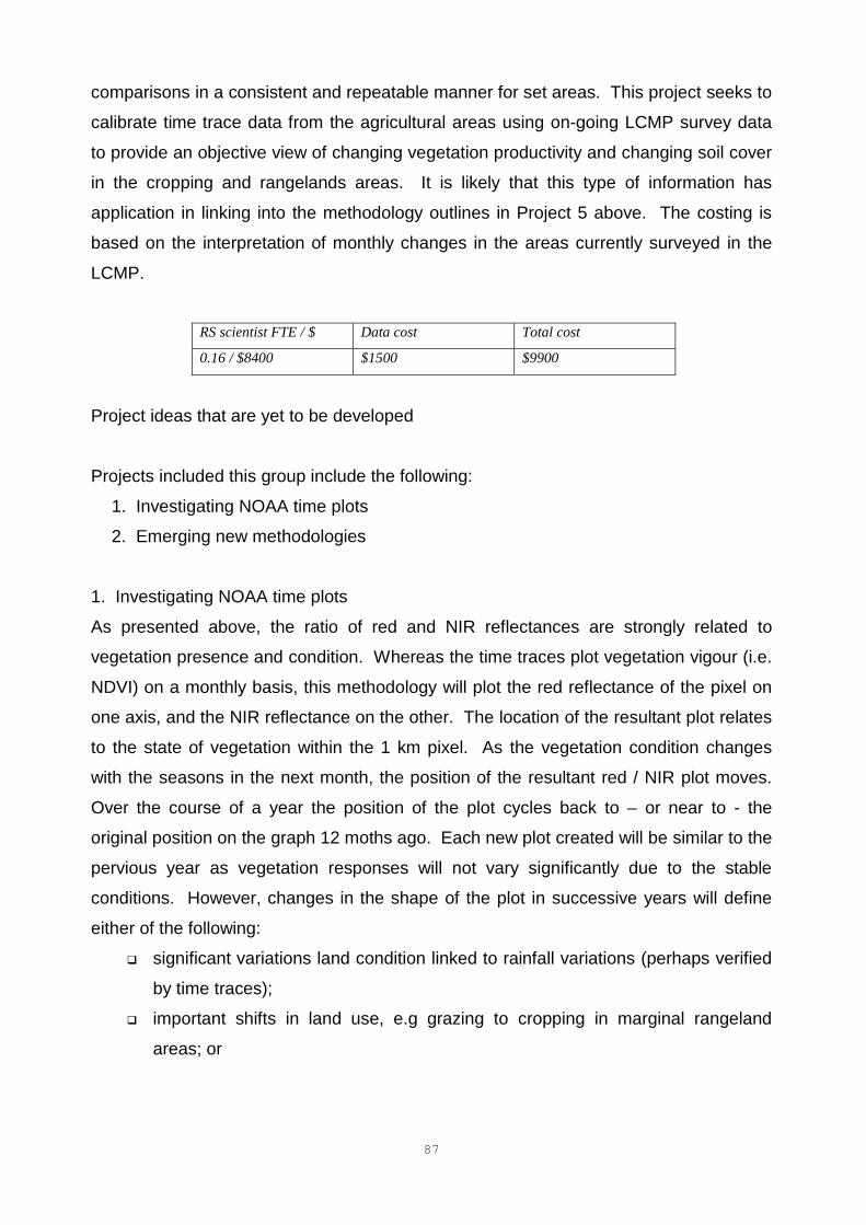
87
comparisons in a consistent and repeatable manner for set areas. This project seeks to
calibrate time trace data from the agricultural areas using on-going LCMP survey data
to provide an objective view of changing vegetation productivity and changing soil cover
in the cropping and rangelands areas. It is likely that this type of information has
application in linking into the methodology outlines in Project 5 above. The costing is
based on the interpretation of monthly changes in the areas currently surveyed in the
LCMP.
RS scientist FTE / $ Data cost Total cost
0.16 / $8400 $1500 $9900
Project ideas that are yet to be developed
Projects included this group include the following:
1. Investigating NOAA time plots
2. Emerging new methodologies
1. Investigating NOAA time plots
As presented above, the ratio of red and NIR reflectances are strongly related to
vegetation presence and condition. Whereas the time traces plot vegetation vigour (i.e.
NDVI) on a monthly basis, this methodology will plot the red reflectance of the pixel on
one axis, and the NIR reflectance on the other. The location of the resultant plot relates
to the state of vegetation within the 1 km pixel. As the vegetation condition changes
with the seasons in the next month, the position of the resultant red / NIR plot moves.
Over the course of a year the position of the plot cycles back to – or near to - the
original position on the graph 12 moths ago. Each new plot created will be similar to the
pervious year as vegetation responses will not vary significantly due to the stable
conditions. However, changes in the shape of the plot in successive years will define
either of the following:
� significant variations land condition linked to rainfall variations (perhaps verified
by time traces);
� important shifts in land use, e.g grazing to cropping in marginal rangeland
areas; or
88
� degradation in land condition – particularly in rangeland areas, e.g. either a
reduced vegetation response as a function of reduced total biomass, or a sharp
vegetation responses (i.e. flushes) as annual species become dominant.
This project will seek to evaluate the utility of these techniques in determining such
events and provide a consistent method to highlight shifts and trends over large areas.
A number of study areas will be selected (e.g. 5 x 2500 sq km) representing different
land uses in different rainfall zones, and time plots will be investigated from the
available NOAA catalogue. Candidate study areas will be selected based on the
availability of historic verification data.
RS scientist FTE / $ Data cost Total cost
0.23 / $11500 $2000 $13500
2. Emerging new methodologies
A number of new opportunities will develop in the coming year(s), based on
technologies / methodologies that are currently emerging. These will offer brand new
opportunities in land condition monitoring e.g. 5, or will enable us to do what is currently
possible better, more efficiently, or cheaper e.g. 3. These developments include:
� MODIS satellite sensor (500 m resolution versus NOAA’s 1 km resolution) for
regional scale monitoring
� ASTER thermal satellite sensor (60 m) for temperature assessment, e.g. for
salinity mapping and crop stress & water use efficiency, etc..
� RADAR DEM technologies for more refined (accurate) DEMs in for whole State
to better support USLE and salinity-type work and salinity work;
� Airborne radiometrics for supporting / verifying erosion assessment;
� Airborne geophysics for monitoring dryland salinity; and
� Hypersepctral remote sensing for salinity through mineral responses.
89
REFERENCESBastin, G.N., Pickup, G. and Stanes, A., 1996, Estimating landscape resilience from
satellite data and its application in pastoral land management, in Rangel. J., 18
(1), 1996, 118 - 35.
Butler P. R. and Dooley, T. J., 1990, Dawson - Paratoo group conservation project; A
revegetation program for pastoral lands, Department of Agriculture, June 1990.
Clarke, K. D., 2000, The utility of multitemporal Landsat 7 ETM+ imagery and
topographic information for the detection of dyland salinity, Honours Thesis,
Adelaide University.
Cyr, L., Bonn, F. and Pesant, A., 1995. Vegetation indices derived from remote sensing
for an estimation of soil protection against soil erosion, Ecological Modelling, 79,
(1995), 277 - 285.
De Jong, S. M., 1994. Derivation of vegetative variables from Landsat TM for modelling
soil erosion, Earth Surface Processes and Landforms, Vol. 19, 165 - 178 (1994).
ERDAS, 1999, ERDAS Field Guide, Fifth Edition, ERDAS Inc.., Atlanta.
Flavel, R. J., 1990. Degradation risk map Cummins, South Australia, Department of
Agriculture, Adelaide.
Furby, S. L., Flavel, R., Sherrah, M. and McFarland, J., 1997, Mapping salinity in the
Upper South East catchment in South Australia: A report for the LWRRDC
project "Mapping Dryland Salinity" (CDM2), CSIRO and PIRSA.
Furby, S. L., Wallace, J. F., Caccetta, P. and Wheaton, G. A., 1995, Detecting and
monitoring salt-affected land: A report from LWRRDC project "Detecting and
monitoring changes in land condition through time using remotely sensed data",
CSIRO, WA.
Hudson, N., 1981. Soil conservation, Batsford Academic and Educational Ltd., London.
Jäger, S., 1992. Modelling regional soil erosion susceptibility using the Universal Soil
Loss Equation and GIS, in: Rickson, R. J. ed. 1992. Conserving Soil Resources:
European Perspectives, CAB International, UK.
Lantieri, D., Dallemand, J. F., Biscaia, R., Sohn, S. and Potter, R. O., 1990. Erosion
mapping using high-resolution satellite data and geographic information system,
FAO RSC Series No. 56, High resolution satellite data series No. 2.
Lillesand, T. M. and Kiefer, R. W., 1987, Remote sensing and image interpretation, 2nd
Ed., John Wiley & Sons.
90
Moore, S., 1990. The Universal Soil Loss Equation for the prediction of soil loss due to
rainfall erosion in South Australia, South Australia Department of Agriculture.
Myeni, R. B., Maggion, S., Iaquinta, J., Privette, J. L., Gobron, N., Pinty, B., Kimes, D.
S., Verstraete, M. M. and Williams, D. L., 1995. Optical remote sensing of
vegetation: modelling, caveats, and algorithms, Remote Sens. Environ., 51: 169
-188, 1995.
Pickup, G., Bastin, G.N. and Chewings, V. H., 1994, Remote sensing-based condition
assessment for nonequilibrium rangelands under large-scale commercial
grazing, in Ecological Applications, 4 (3), 1994, pp 497 - 517.
Pickup, G., Bastin, G.N. and Chewings, V. H., 1998, Identifying trends in land
degadation in non-equilibrium rangelands, in Journal of Applied Ecology, 1998,
35, 365 - 377.
Shao, Y. and Leys, J. F., 1997. Wind erosion assessment and prediction using dynamic
models and field experiments, in Munro, R. K. and Leslie, L. M., eds., 1997.
Climate prediction for agricultural and resource management: Australian
Academy of Science Conference, Canberra, 6 - 8 May 1997. Bureau of
Resource Sciences, Canberra.
Thomas, M., 1997, DIY remote sensing, Mapping Awareness, Vol. 11, Number 1, 1997.
Thomas, M., 1998, Video-based remote sensing in woody savanna condition
assessment; for the North West Parks Board, CSIR, 1998.
Thomas, M., 2000, An application of SPOT XS in wind and water erosion susceptibility
modelling in the cropping areas of South Australia, in Procs. Of 10th Australasian
Remote Sensing and Photogrammetry Conference, Adelaide, August 2000.
USDA, 1997. Predicting soil erosion from water: A guide to conservation planning with
the Revised Universal Soil Loss Equation (USLE), Agriculture handbook No. 703,
Agricultural Research Service, Washington.
Wischmeier, W. H. and Smith, D. D., 1978. Predicting rainfall erosion losses. A guide
to conservation planning. Agric. Handbook No. 537. US Dept. Agric.:
Washington, D.C..

91
APPENDIX 1: SOME IMPORTANT REMOTE SENSINGPRINCIPLES
Remote sensing involves the diagnosis of the characteristics of substances / surfaces at
a distant location. It involves interpretation of reflected surface energy measured
through remote sensing sensors. Some sensors operate with systems that measure
energy that is derived from reflected sunlight. These are known as “passive” or “optical”
remote sensing systems. Other sensors measure reflected energy from their own
emission systems. These are known as “active” remote sensing systems. RADAR is
the most common active type of system. The following section discusses this topic in
more detail.
Energy sources
The energy measured by remote sensing sensors is derived from the electromagnetic
spectrum (EMS). The EMS is comprised of a naturally occurring, continuous range of
lengthening wavelengths, ranging from ultra violet (UV) (short wavelength); visible; near
infrared (NIR); mid-infrared (MIR); thermal; microwaves (RADAR) (long wavelength).
The energy reflected by substances is highly diagnostic of their composition. This is
because particular atoms, molecules and textures absorb energy at highly specific
wavelengths, with the rest ending up being reflected. The composition of the reflected
light is known as the “reflectance spectra”. The compositions of healthy green leaves
absorb energy from much of the visible EMS except for green light. Green light thereby
dominates the reflectance spectra of healthy leaves and is why they are seen as green.
Many substances have multiple absorption regions throughout the EMS, and detailed
knowledge of the location of these absorption regions are used as diagnostic indicators
to identify things like mineralogy, vegetation health, vegetation species, and biomass.
Multispectral remote sensing sensors have been developed to measure the multiple
diagnostic absorption zones of substances by operating in many specific ranges, or
bands of the EMS. Some of the most commonly used multispectral system sensors that
have been developed for natural resources applications are Landsat ETM+, SPOT XS,
and NOAA AVHRR. These systems feature bands that are highly diagnostic of natural
terrestrial substances such as vegetation and minerals. They measure seven, four and
four bands respectively.
92
Hyperspectral sensors are sensitive to a much larger number of bands that operate in
extremely narrow ranges of wavelengths. They are used as highly diagnostic tools that
are capable of very detailed discriminations. They are used to differentiate between
various mineral alteration states and subtleties in vegetation health. The airborne
HYMAP sensor is one such hyperspectral systems and operates in greater than 170
bands ranging from visible to thermal wavelengths.
Sensors vary in capability according to the wavelength of their particular energy source.
Energy sources that have longer wavelengths that penetrate deeper into a subsurface
can reveal more information on the nature of the substances within. The shorter
wavelengths however have a limited penetration capacity and can only effectively reveal
surface information.
RADAR systems have longer wavelengths that are capable of penetrating cloud and will
perform in total darkness as they operate using their own reflected energy sources.
Longer wavelength RADAR systems (e.g. P and L band) may also penetrate vegetation
and soils to reveal, e.g. biomass and structural information of plants, and moisture and
profile information in soils. Shorter wavelengths (i.e. X and C band) can be used to
reveal surface and textural information such as canopy and soil surface textures.
Issues of image scale and quality
Remote sensing images are pictures comprised of a 2D array of picture elements
(pixels) that represent the reflectance from corresponding areas on the ground. The
type of systems used to produce them determines the image resolution and study area
dimensions. “High resolution” remote sensing systems capture a high quality of colour,
hue and tonal information about objects and surfaces on the ground. When these are
combined, life-like patterns are revealed and recognised on the ground in an intuitive
process that forms the basis of air photo interpretation (API). Airborne remote sensing
systems are synonymous with high-resolution imagery like air photography. These
systems range in resolution between 30 cm to 5 m. However, their high visual quality is
achieved at the expense of area coverage on the ground due to technical trade-offs
between the various elements within the whole imaging system. For example, with
lens-based airborne systems, a fixed relationship exists between flying height, lens
settings, image resolution and area ground coverage, i.e. the higher the aircraft flies
without changing the lens setting, the lower the image resolution, but greater the area
coverage.
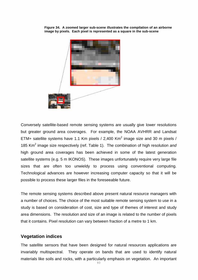
93
Figure 34. A zoomed larger sub-scene illustrates the compilation of an airborneimage by pixels. Each pixel is represented as a square in the sub-scene
Conversely satellite-based remote sensing systems are usually give lower resolutions
but greater ground area coverages. For example, the NOAA AVHRR and Landsat
ETM+ satellite systems have 1.1 Km pixels / 2,400 Km2 image size and 30 m pixels /
185 Km2 image size respectively (ref. Table 1). The combination of high resolution and
high ground area coverages has been achieved in some of the latest generation
satellite systems (e.g. 5 m IKONOS). These images unfortunately require very large file
sizes that are often too unwieldy to process using conventional computing.
Technological advances are however increasing computer capacity so that it will be
possible to process these larger files in the foreseeable future.
The remote sensing systems described above present natural resource managers with
a number of choices. The choice of the most suitable remote sensing system to use in a
study is based on consideration of cost, size and type of themes of interest and study
area dimensions. The resolution and size of an image is related to the number of pixels
that it contains. Pixel resolution can vary between fraction of a metre to 1 km.
Vegetation indices
The satellite sensors that have been designed for natural resources applications are
invariably multispectral. They operate on bands that are used to identify natural
materials like soils and rocks, with a particularly emphasis on vegetation. An important
94
development in multispectral remote sensing has been the discovery that mathematical
combinations of the visible red and near NIR spectral bands can be used to determine
the presence and condition of vegetation, or indeed, the absence of vegetation. The
results of these band combinations are called vegetation indices (VIs). The most
commonly used VI is the “Normalised Difference Vegetation Index” (NDVI), and is
calculated according to the following formula:
NDVI = (Band 2 - Band 1) / (Band 2 + Band 1) * scaling factor
According to Lillesand and Kiefer (1987), healthy vegetation have high VIs because of
high NIR and low red reflectances. Conversely, materials like clouds, water, soil, sand,
and other non-vegetated surfaces show high red and low NIR relative reflectances, and
thus these have low-to-zero value vegetation indice values. The indices are usually
scaled for display purposes1.
Assumptions and caveats in remote sensing
The issues relating to the use of digital remote sensing in natural resources include
some important assumptions and caveats involved in the application of these
technologies. According to Myneni, et al (1995) “the central hypothesis in remote
sensing is that radiation reflected from a surface carries information about the state of
the surface. The appropriation of signal characteristics with surface properties is
complicated for one can never measure in isolation the desired cause and effect in the
system.” This implies that there are a number of environmental factors that exert an
effect on the spectral responses of a surface cover. These environmental factors are
described below.
� Bidirectional effects:–The spectral red and NIR band scattering are not necessarily
uniform at the top of canopies because the contrasts between shaded and sunlit
1 The scaling factor is applied in order to maximise the distribution of digital values within the NDVI
image, exploiting the full digital dynamic range. For example, a scaled 8 bit image would show a
distribution of digital numbers ranging from zero (black; no vegetation response at all) to 256 (white;
maximum vegetation response).
95
elements of the canopy influence the NIR band more than the red band. These effects
may cause variations in absolute band ratio values per coverage area. Additionally,
“hot spots” may occur where scattering is uniform in the bands; with maximum
reflectances, i.e. the hot spots, may occur in the retro-solar direction. From such
observations, it may be seen that variations in measurements may not necessarily be
attributable to variations in vegetation.
� Atmospheric effects:– The red and NIR band scattering are not necessarily
uniform throughout the atmosphere as these bands are differentially scattered due to
various atmospheric vapour, chemicals and particles.
� Plant structural effects:– Leaf size distribution and canopy height determine the
amplitude and width of the top-of-canopy shown in the spectral response profile.
However, within that profile, changing leaf orientation exerts an affect on the absolute
reflectance values within these profiles that are non-linear across the spectral profile.
� Background or soil effects:– Reflectance at the top-of-canopy is a composite of
the responses due to vegetation matter and soil. Thus, parameters such as leaf area
index (LAI) are effected by changing soil albedo, e.g. the uncorrected spectral response
of a bright soil, will apparently reduce the LAI value for a given canopy cover compared
to a darker soil.
� Adjacency effects:– This occurs where some reflectance pixel values are affected
by “spectral contamination” due to atmospheric scattering. Neighbouring pixels can
show contrast with increased scattering, and is more significant as pixel resolution
increases.
� Non-linear mixing:– It is assumed that, for a pixel containing two different cover
classes (e.g. soil and plant), the resulting spectral response is a combination of the
spectral reflectances of each class. Further, it is assumed that each of the cover-type’s
contribution to the overall spectral response is linear, according to proportion coverage
within the pixel, i.e., linear mixing. However, in reality non-linear mixing occurs because
of the occasional multiple reflectance paths of light. This effects the amplitude and
wavelength of the response inside the pixel, e.g. light bouncing between soil and under-
canopy prior to transmittance to the sensor.
96
� Topographic effects:– The effects of topography in remote sensing are two-fold.
Firstly, slope, aspect influence the amount of light incident on a surface where
steepness and sun aspect cause varying degrees of shadow. Here altitude also
influences observations by compounding the effect of light transmitted and reflected
through the atmosphere.
Secondly the amount of light reflected to the sensor is determined by the angle of the
surface relative to the location of the sensor. This causes additional complications to
occur through topographical effects of the response of spectra of interest at given
satellite ground resolutions. The effect of slope on the spectral mix within a pixel can be
extremely complex and can result in misreading of the ground surface area under the
sensors instantaneous field of view. This can result in under or over estimating due to
foreshortening of the view. For example when two pixels each covering a ground
surface where soil cover and canopy cover are equal, the readings will differ between
these pixels. Discrepancies will occur when one of these pixel’s surface slope is facing
away from the relative position of the sensor and the other pixel’s surface slope is facing
towards the relative position of the sensor. If the ground surface slope facing away from
the relative position of the sensor the pixel would register a higher ratio for the canopy
component as it would appear to be denser. Conversely the pixel covering the ground
surface area with the slope facing towards the relative position of the sensor would
register a higher ratio for the soil component, as more ground would be exposed at that
angle of view.
97
APPENDIX 2: AIRBORNE REMOTE SENSINGOPERATING PRINCIPLES
This section provides an overview of important principles that ensure successful
acquisitions of high quality, user-defined imagery.
Airborne remote sensing surveys involve finding the optimal compromise between
operational affordability and the suitability of the image specifications to fit the image /
information requirements. It is advisable to determine the minimum resolution required
for the entire project before beginning. (i.e. chenopod bush classification at 30 cm
resolution or gully erosion mapping at 1.5 m). The minimum resolution is needed to
plan the flight survey where the camera settings are fixed accordingly. Fortunately this
can be easily determined, because image quality is a function of the following elements
of an airborne remote sensing survey:
� camera resolution;
� lens focal length;
� CCD array size; and
� height above ground.
The spatial resolution of airborne remote sensing imagery is determined through a fixed
formula between these four elements. As with the principles governing
photogrammetry, for a fixed focal length, as the height of the aircraft increases so does
the area of ground covered by the image at the expense of the resolution. This
relationship is expressed through the following formula (after: USDA, 1992):
H = (D * f) / I
Where,
H = height above ground
D = distance on ground (image dimensions)
f = focal length
I = image area (CCD physical dimensions) - and is remains fixed for any camera. (See
Figure 2)

98
Figure 35. The fixed relationships between lens settings and flying heights inairborne remote sensing survey and photogrammetry, after USDA (1992).
The resolution of the image can be calculated by dividing D by the number of pixelsalong the corresponding axis of the CCD, thus:
R = D / A
Where,
R = pixel resolution
D = distance on ground (image dimensions)
A = the number pixels along the axis.
As the relationship between the flying height (H) and swath length (D) is constant at a
fixed focal length, then D can be calculated through using a ratio, e.g. where D is 400 m
and H is 500 m, then the D-to-H ratio is expressed through the following formula:
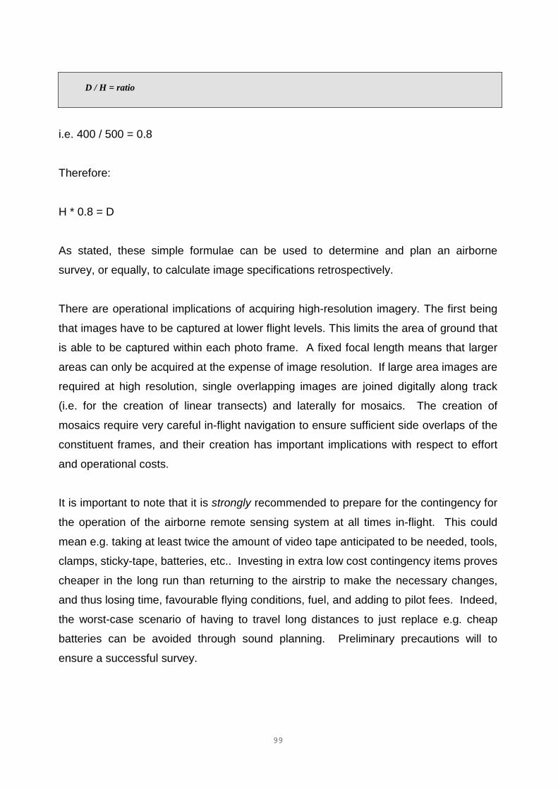
99
D / H = ratio
i.e. 400 / 500 = 0.8
Therefore:
H * 0.8 = D
As stated, these simple formulae can be used to determine and plan an airborne
survey, or equally, to calculate image specifications retrospectively.
There are operational implications of acquiring high-resolution imagery. The first being
that images have to be captured at lower flight levels. This limits the area of ground that
is able to be captured within each photo frame. A fixed focal length means that larger
areas can only be acquired at the expense of image resolution. If large area images are
required at high resolution, single overlapping images are joined digitally along track
(i.e. for the creation of linear transects) and laterally for mosaics. The creation of
mosaics require very careful in-flight navigation to ensure sufficient side overlaps of the
constituent frames, and their creation has important implications with respect to effort
and operational costs.
It is important to note that it is strongly recommended to prepare for the contingency for
the operation of the airborne remote sensing system at all times in-flight. This could
mean e.g. taking at least twice the amount of video tape anticipated to be needed, tools,
clamps, sticky-tape, batteries, etc.. Investing in extra low cost contingency items proves
cheaper in the long run than returning to the airstrip to make the necessary changes,
and thus losing time, favourable flying conditions, fuel, and adding to pilot fees. Indeed,
the worst-case scenario of having to travel long distances to just replace e.g. cheap
batteries can be avoided through sound planning. Preliminary precautions will to
ensure a successful survey.
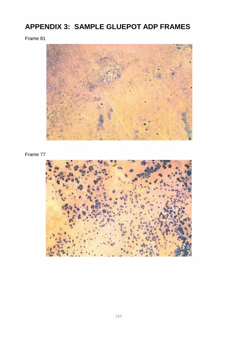
100
APPENDIX 3: SAMPLE GLUEPOT ADP FRAMESFrame 81
Frame 77
101
Frame 156
Frame 119
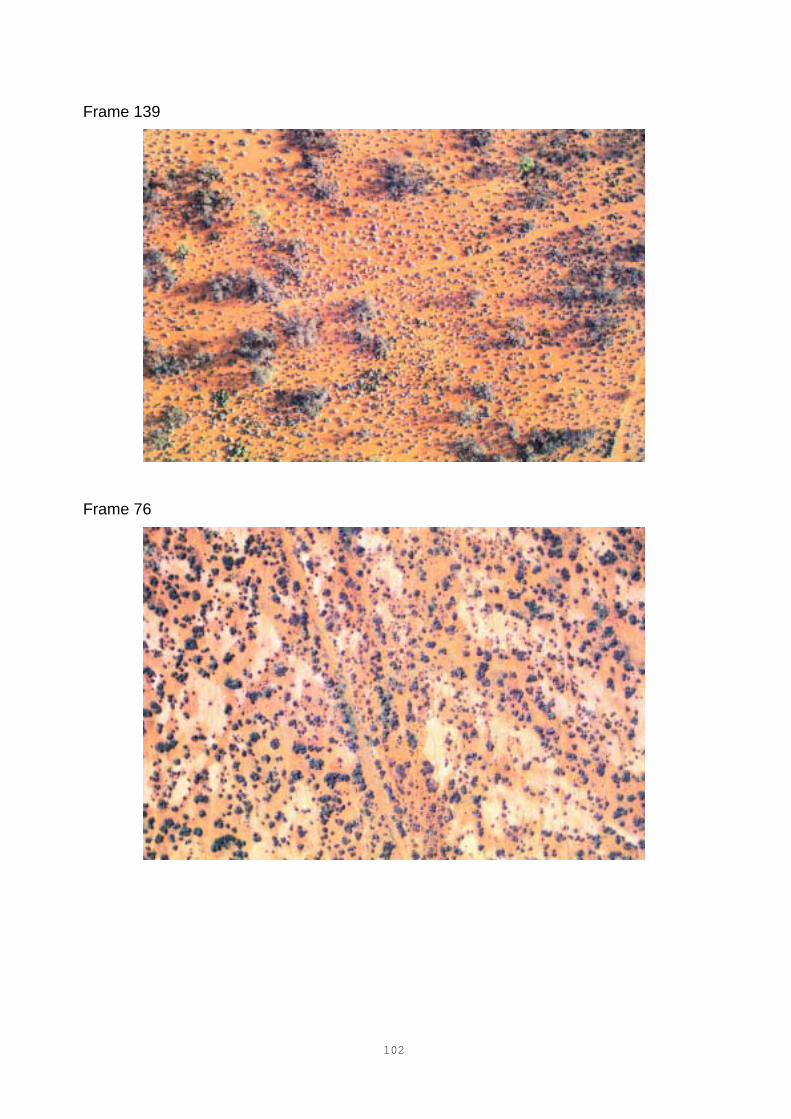
102
Frame 139
Frame 76