report series in geophysics

UNIVERSITY OF HELSINKI FACULTY OF SCIENCE DEPARTMENT OF PHYSICS

REPORT SERIES IN GEOPHYSICS No. 75

DATABASE-WIDE STUDIES ON THE VALIDITY OF THE

GEOCENTRIC AXIAL DIPOLE HYPOTHESIS IN THE PRECAMBRIAN

Toni Veikkolainen Helsinki 2014

Supervisor:

Prof. (emeritus) Lauri J. Pesonen Division of Materials Physics Department of Physics University of Helsinki Helsinki, Finland Pre-examiners: Prof. Rob Van der Voo Docent (emeritus) Heikki Nevanlinna Department of Earth and Environmental Finnish Meteorological Institute Sciences Helsinki, Finland University of Michigan Ann Arbor, Michigan, USA Opponent: Custos: Ph.D. Sergei Pisarevsky Prof. Ilmo Kukkonen School of Earth and Environment Division of Materials Physics University of Western Australia Department of Physics Perth, Australia University of Helsinki Helsinki, Finland

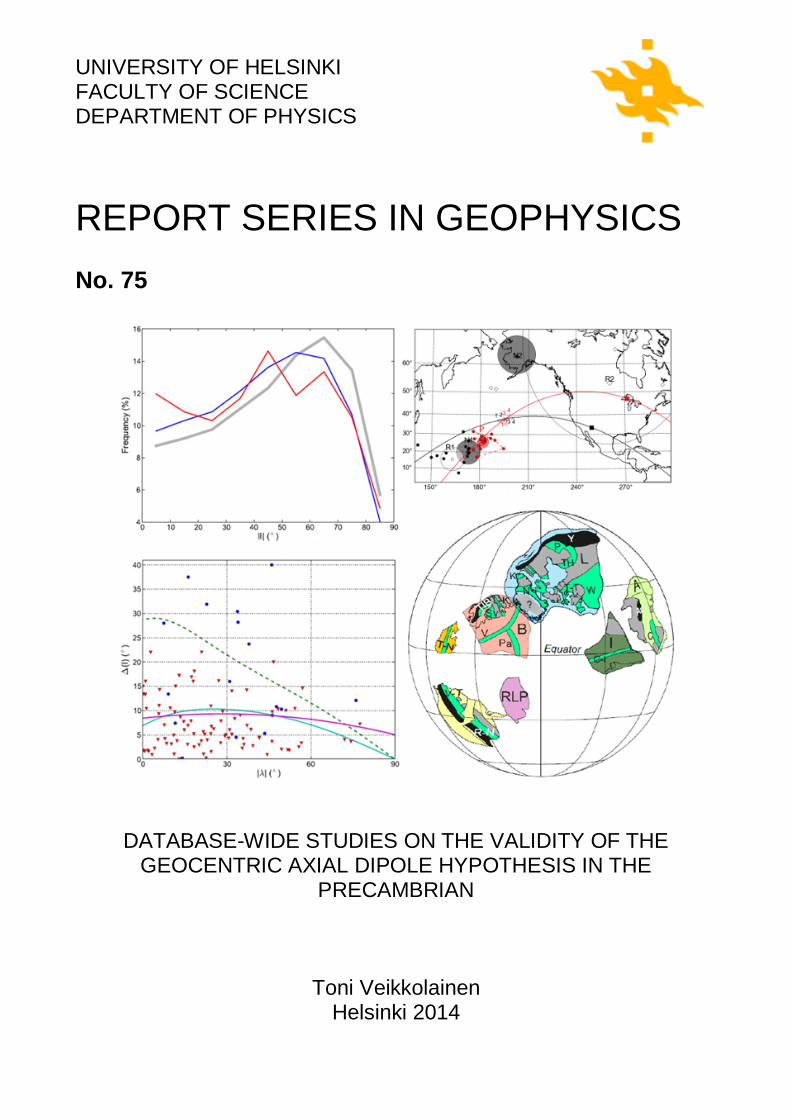
Cover picture: Methods of research applied include inclination frequency analysis (upper

left), calculation of the shift of paleomagnetic poles due to zonal multipoles (upper right), reversal asymmetry analysis (lower left) and paleogeographic reconstructions (lower right).

ISBN 978-951-51-0087-0 (printed version) ISSN 0355-8630

Helsinki 2014 Unigrafia

ISBN 978-951-51-0088-7 (pdf-version)

Helsinki 2014 http://ethesis.helsinki.fi

Database-wide studies on the validity of the Geocentric AxialDipole hypothesis in the Precambrian

Toni Veikkolainen

ACADEMIC DISSERTATION IN GEOPHYSICS

To be presented, with the permission of the Faculty of Science of the University of Helsinki forpublic criticism in the Auditorium D101 of Physicum building at Kumpula campus, Gustaf

Hällströmin katu 2a, on October 10th, 2014, at 12 o’clock noon.

Nomenclature

Unless otherwise noted in the text, symbols and abbreviations have been used as follows.Units are in SI system.

AF Alternating (magnetic) fieldAPW(P) Apparent polar wander (path)CHAMP Challenging Minisatellite PayloadChRM Characteristic remanent magnetizationCRM Chemical remanent magnetizationEGT European Geotraverse ProjectGa Billion years (ago)GAD Geocentric Axial DipoleGPMDB Global Paleomagnetic DatabaseIAGA International Association of Geomagnetism and AeronomyIMAGE International Monitor for Auroral Geomagnetic EffectsLIP Large igneous provinceLIRM Lightning-induced remagnetizationMa Million years (ago)MD Multidomain (grain size)MV Modified Van der Voo quality gradingND Non-dipolar (field)NRM Natural remanent magnetizationPSD Pseudo-single domain (grain size)PSV Paleosecular variationSD Single domain (grain size)SQUID Superconducting Quantum Interference DeviceTAFI Time-Averaged Field InitiativeTCRM Thermochemical remanent magnetizationTPW True polar wanderTRM Thermoremanent magnetizationVADM Virtual axial dipole momentVDM Virtual dipole momentVGP Virtual geomagnetic poleVRM Viscous remanent magnetization

A95 Radius of the Fisherian 95 % confidence circle for the mean paleomagnetic pole [◦]Antip Antiparallelism angle between normal and reversed field directions [◦]B Total geomagnetic field vector [T]c Radius of the core of the Earth [m]d(I) Inclination anomaly, the difference between observed I and I expected from GAD model [◦]D Geomagnetic declination [◦]Dm Declination of NRM [◦]f Sedimentary inclination flattening factor (dimensionless)F Intensity of the geomagnetic field [Am−1]F0 Intensity of the geomagnetic field at the equator [Am−1]H Horizontal geomagnetic field vector [T]g0

1 Geocentric axial dipoleg0

2 Geocentric axial quadrupole (G2= g02/g0

1)g0

3 Geocentric axial octupole (G3= g03/g0

1)g0

4 Geocentric axial hexadecapole (G4= g04/g0

1)I Geomagnetic inclination [◦]Im Inclination of NRM [◦]J Electric current density [Am−2]

m Spherical harmonic orderM Dipole moment [Am2]n Spherical harmonic degreeQ Königsberger ratio (dimensionless)r Distance from the magnetic sources or distance from the center of the Earth [m]R Radius of the Earth [m]U Magnetic scalar potential [T m2]X Geomagnetic field vector pointing towards the geographic north [T]X 2 Chi-square test statistic (dimensionless)Y Geomagnetic field vector pointing towards the geographic east [T]Z Vertical geomagnetic field vector [T]α95 Radius of the Fisherian 95 % confidence circle for the mean direction [◦]∆(D) Antiparallelism angle of normal and reversed declinations [◦]∆(I) Antiparallelism angle of normal and reversed inclinations [◦]θ Magnetic colatitude [◦]κ Fisherian concentration parameter for directional data (dimensionless)λ Geographic (paleo)latitude [◦]λp Latitude of the paleomagnetic pole [◦]λs Latitude of the sampling site [◦]µ0 Vacuum permeability [T mA−1]ρ Spatial resolution of the spherical harmonic model [m]φ Geographic longitude [◦]φp Longitude of the paleomagnetic pole [◦]φs Longitude of the sampling site [◦]χv Volume susceptibility (dimensionless)

Abstract

A branch of science concentrated on studying the evolution of the Earth’s magnetic fieldhas emerged in the last half century. This is called paleomagnetism, and its applications in-clude calculations of field directions and intensity in the past, plate tectonic reconstructions,variations in the conditions in the Earth’s deep interior and the climatic history. With the in-creasing quantity and quality of observations, it has been even possible to construct modelsof conterminous continent blocks, or supercontinents, of the Pre-Pangaea time. These arecrucial for the understanding of the evolution of our planet from the Archean to today.

Paleomagnetists have traditionally heavily relied on the theory that when averaged over aperiod long enough, the Earth’s magnetic field can be approximated as being equivalent tothat generated by a magnetic dipole located at the center of the Earth and aligned with theaxis of rotation. The credibility of this GAD (Geocentric Axial Dipole) hypothesis is strongestin the geologically most recent eras, such as most of the Phanerozoic and notably in the last400 million years. Attempts to get an adequate view of the magnetic field in the Earth’s ear-lier history have for a long time been challenged by the reliability limitations of Precambrianpaleomagnetic data. With the absence of marine magnetic anomalies, observational dataneed to be gathered from terrestrial rocks, notably those formed within cratonic nuclei, theoldest and most stable parts of continents.

To answer the call for a concise and comprehensive compilation of paleomagnetic data fromthe early history of the Earth, this dissertation introduces a unique database of over 3300Precambrian paleomagnetic observations worldwide. The data are freely available at theserver of the University of Helsinki (http://h175.it.helsinki.fi/database) and canbe accessed via an online query form. All database entries have been coded according totheir terranes, rock formation names, ages, rock types and paleomagnetic reliabilities. Anew modified version of the commonly applied Van der Voo (MV) classification criteria forfiltering the paleomagnetic data is also presented, along with a novel method for binning theentries cratonically to revise the previously employed way of applying binning via a simpleevenly spaced geographic grid. Besides compiling data, tests of the validity of the GADhypothesis in the Precambrian have been conducted using inclination frequency analysisand asymmetries of magnetic field reversals.

Results from two self-contained tests of the GAD hypothesis suggest that the time-averagedPrecambrian geomagnetic field may include the geocentric axial quadrupole (g0

2) and thegeocentric axial octupole (g0

3), but both with strengths less than 10% of g01 , the quadrupole

perhaps being smaller than the octupole. In no other study a model so close to GAD has beenreasonably fitted to the Precambrian paleomagnetic data. The weakness of the non-dipolarcoefficients required also implies that no substantial adjustments need to be made to thenovel models of Precambrian continental assemblies (supercontinents), such as the Paleo-Mesoproterozoic Columbia (Nuna) or the Neoproterozoic Rodinia. Although the supercon-tinent science still has plenty of uncertainty, it is more plausibly caused by the geologicalincoherence of the data and the lack of precise age information rather than by long-livednon-dipolar geomagnetic fields.

i

http://h175.it.helsinki.fi/database

Acknowledgements

The research presented here is a continuation to my Master’s thesis The validity of thedipole model of geomagnetic field according to inclination distribution (University of Helsinki,November 2010). For the completion of the work, I’m grateful especially to my supervisor,professor Lauri. J. Pesonen, who provided me a challenging topic of research and also gaveme priceless remarks and suggestions to improve the way I present my results. In addition,advice from M.Sc. (Tech.) Kimmo Korhonen from the Geological Survey of Finland (GSF)has been crucial. He provided me the original versions of the Python

TMprograms, which I

later upgraded and also developed new programs to better suit my own research purposes.I am also indebted to Dr. Satu Mertanen (GSF), who made a lot of effort to update thepaleomagnetic data of Fennoscandia for the finalization of PALEOMAGIA, a unique globaldatabase of Precambrian paleomagnetic information. The collaboration with professor DavidA.D. Evans (Yale University) has been fruitful during all phases of the project. Special thanksgo to him for arranging our visit to Yale in January 2013.

I wish to thank all Ph.D. students and postdoctoral researchers at the Division of the Geo-physics and Astronomy of the University of Helsinki. Special thanks go to Dr. Michal Bucko,M.Sc. Robert Klein, Dr. Johanna Salminen and Dr. Tomas Kohout for interesting scientificdiscussions and all the time spent together. Another memorable events during my Ph.D. stud-ies include organizing an international scientific conference (Supercontinent Symposium2012), and a national biannual geophysical colloquim (Geophysics Days 2013) in Helsinki.The funding provided by the Research Foundation of the University of Helsinki and OskarÖflund Foundation was important in the first year of my postgraduate studies. Thereafter,the continuation of the work owes much to professors Juhani Keinonen and Hannu Koskinen,the previous and current heads of the Department of Physics, who gave me an opportunityto a two-year employment at the division. Finally, I thank my relatives and friends for theirenduring support.

ii

Publications

The main results of the research are included in five papers, which are referred to in thetext by their Roman numerals. Methods used for the studies were first presented in Paper I,which also introduces the main paleogeographic applications of the data, including Precam-brian supercontinent models. Papers II-III deal with estimating the validity of the GAD andPaper IV describes a newly improved way to average paleomagnetic data spatially. Paper Vgives an overview of the paleomagnetic database built for conducting the research describedin four other papers.

Papers I and IV are reprinted with the permission of the Geophysical Society of Finland.Papers II and III are reprinted with the permission of Reed Elsevier.Paper V is reprinted with the permission of Springer Verlag.

Paper I: Pesonen, L.J., Mertanen, S. and Veikkolainen, T., 2012. Paleo-Mesoproterozoic Super-continents - A Paleomagnetic View. Geophysica 48, 5-47.

Toni Veikkolainen participated in the compilation of paleomagnetic data, calculated the in-clination distributions used to estimate the validity of the Geocentric Axial Dipole (GAD)hypothesis and applied the results to the paleomagnetic reconstructions done by the twoother authors. He was partly responsible for drawing the illustrations. He contributed ac-tively to the paper before and after its review process.

Paper II: Veikkolainen, T., Pesonen, L.J., Korhonen, K. and Evans, D.A.D., 2014. On the low-inclination bias of the geomagnetic field. Precambrian Research 244, 23-32.

Toni Veikkolainen was the first author. He collected, analyzed and filtered the paleomag-netic data, upgraded the Python software necessary for analysis, checked the coherence ofthe paleomagnetic data, calculated the inclination distributions and compared the resultswith those achieved from previous studies. He was responsible for writing and revising themanuscript.

Paper III: Veikkolainen, T., Pesonen, L.J. and Korhonen, K., 2014. An analysis of geomagneticfield reversals supports the validity of the Geocentric Axial Dipole (GAD) hypothesis in the Pre-cambrian. Precambrian Research 244, 33-41.

Toni Veikkolainen was the first author. He calculated paleomagnetic Fisher statistics fornormal- and reversed-polarity data, compiled the results to a table, analyzed, and whennecessary, removed duplicate observations. He developed Python scripts necessary for calcu-lations, sketched the illustrations, wrote the manuscript and replied to the review comments.

Paper IV: Veikkolainen, T., Korhonen, K. and Pesonen, L.J., 2013. On the spatial averaging ofpaleomagnetic data. Geophysica 50, 49-58.

Toni Veikkolainen was the first author. He was responsible for constructing the Precambrian

iii

paleomagnetic database essential for the study, developing the simulation script originallywritten by the second author to suit this study, preparing and formatting the manuscript,and sketching the illustrations.

Paper V: Veikkolainen, T., Pesonen, L.J. and Evans, D.A.D., 2013. PALEOMAGIA: A PHP/MYSQLdatabase of the Precambrian paleomagnetic data. Studia Geophysica et Geodaetica 58, 425-441.

Toni Veikkolainen was the first author. He was in charge of maintaining the spreadsheet datathe time of 2.5 years before its transfer to the database server, validated the entries usinglatest paleomagnetic and supplementary geological information available, was responsibleof making necessary statistical calculations and developed Python programs for sketchingpurposes. He was entrusted with the technical part of the database project, including thedevelopment of the database website, setting up the PHP/MYSQL based search engine, andthe documentation of the project.

iv

Contents

1 Introduction 11.1 Fundamentals of geomagnetic fields . . . . . . . . . . . . . . . . . . . . . . . . . . 21.2 Precambrian data and paleointensity . . . . . . . . . . . . . . . . . . . . . . . . . . 111.3 Paleomagnetic poles . . . . . . . . . . . . . . . . . . . . . . . . . . . . . . . . . . . . 151.4 The PALEOMAGIA database and outline of research . . . . . . . . . . . . . . . . . 18

1.4.1 Motivation and construction . . . . . . . . . . . . . . . . . . . . . . . . . . . 181.4.2 Structure of the database . . . . . . . . . . . . . . . . . . . . . . . . . . . . . 211.4.3 Applying the data to study the evolution of the geomagnetic field . . . . 22

2 Inclination frequency analysis 282.1 Data and modelling . . . . . . . . . . . . . . . . . . . . . . . . . . . . . . . . . . . . . 292.2 Binning simulations . . . . . . . . . . . . . . . . . . . . . . . . . . . . . . . . . . . . . 292.3 Results and conclusions . . . . . . . . . . . . . . . . . . . . . . . . . . . . . . . . . . 31

3 Reversal asymmetry analysis 343.1 Data and modelling . . . . . . . . . . . . . . . . . . . . . . . . . . . . . . . . . . . . . 343.2 Results and conclusions . . . . . . . . . . . . . . . . . . . . . . . . . . . . . . . . . . 36

4 Discussion 38

References 50

v

1 Introduction

Magnetism is one of the driving forces of the nature, and present in the microscopic andplanetary scale alike. Most large bodies of the solar system maintain an internal magneticfield, following Maxwell’s equations and behaving according to the dynamo principle. OurEarth, with its large, partly molten iron-nickel core, has electric currents in the scale ofgiga-amperes (109A) and sustains a dynamo-generated magnetic field at a depth of 2900to 5200 km below its surface. This internal field, tilted 11◦ about the axis of rotation,contributes to ca. 99% of the total field content and is driven by the motions of electricallyconducting iron-nickel alloy in the planet’s outer core. If the motions of this self-sustainingdynamo disappeared, the field would pass away due to the Ohmic dissipation, the fate ofthe primordial magnetic fields of the Moon [Stegman et al., 2003] and Mars [Weiss et al.,2002].

The scientific interest towards the geomagnetic field increased in the 17th century, after thepublication of William Gilbert’s (1544-1603) De Magnete, with the leading principle that theEarth itself sustains a magnetic field. Before this, Petrus Peregrinus de Maricourt (Peter thePilgrim of Maricourt) had noticed that the compass needle points to the direction of thecelestial pole, but the source of the magnetism was unknown. Cristopher Columbus, whencrossing the Atlantic, noticed that the deviation between the compass direction and the lo-cation of the Pole Star was larger in the west than in the east, but he could not associatethe phenomenon with the magnetic declination. Thereafter, compasses were used not justfor navigation but also for geophysical measurements, and the concept of a magnetic polewas vaguely established. Nonetheless, the theory of a mainly dipolar geomagnetic field wasfar from self-evident. For instance, Edmund Halley (1656-1742), famous for his comet, un-derstood the changing compass direction in the course of time (i.e. concept of geomagneticdeclination). On the other hand, he suggested that the number of geomagnetic poles is four,and this assumption was not abandoned until the early 19th century [Hansteen, 1819]. Fora detailed historical view on geomagnetism and paleomagnetism, see e.g. Courtillot andLe Mouël [2007].

Albert Einstein (1879-1955), after writing his paper on special relativity in 1905, regardedthe origin of the geomagnetic field as one of the five unsolved problems in physics. Thesituation remained mostly unchanged until the development of the magnetohydrodynamictheory by Walter M. Elsasser (1904-1991), a German-born American physicist and biolo-gist [Elsasser, 1939], and Hannes Alfvén (1908-1955), a Swedish plasma physicist [Alfvén,1950]. The evolution of the field, however, was much of a mystery before the introduction ofpaleomagnetic method. Remnants of the ancient geomagnetic field were observed to survivein certain rocks and other geological material and it was suggested that the data can be usednot only to trace the geomagnetic field back in time but also to test the continental drift and

1

1.1 Fundamentals of geomagnetic fields 1 INTRODUCTION

hypotheses of polar wander [Irving, 2005, Runcorn, 1956]. This was the birth of a branch ofscience with unforeseen applications to paleogeographic reconstructions, magnetic dating,economic geology and climatic history of our planet, etc. In the last decades, theories thatthe Earth has possessed an internal magnetic field for at least 3.5 Ga have gained supportfrom observational data from Australia and South Africa [Yoshihara and Hamano, 2004].

The interpretation of paleomagnetic observations has generally been based on the so-calledGeocentric Axial Dipole (GAD) hypothesis [Hospers, 1954]. It states that the temporally av-eraged geomagnetic field is oriented in the direction of the axis of rotation, passes the centerof the planet, and no quadrupolar, octupolar or higher-order terms are necessary to explainits structure. The general motivation towards the GAD hypothesis was based on the fact thatthe north and south poles of the historical geomagnetic field mapped around the current ge-ographic pole [Cox and Doell, 1960]. However, all combinations of zonal harmonics (axialdipole g0

1 , axial quadrupole g02 and axial octupole g0

3) produce a distribution of poles of thatkind. Runcorn [1954] stated that the Coriolis force, being responsible for the pattern of fluidflow inside Earth, should produce an axisymmetric field, but he was unable to prove that thefield is solely dipolar. Therefore he discussed the possible existence of other axially symmet-ric multipoles, too [Runcorn, 1959]. It is evident that no geomagnetic field model withoutnon-zonal multipoles can be used for modelling the instantaneous field, due to Cowling’santidynamo theorem [Cowling, 1955] which does not allow an axially symmetric current toproduce an axisymmetric magnetic field via dynamo action. The application of GAD hypoth-esis is therefore restricted to the temporally averaged field which can be fruitfully describedvia spherical harmonics rather than via solutions of dynamo equations.

1.1 Fundamentals of geomagnetic fields

An axially symmetric geomagnetic field can be described mathematically in a convenientway, since no transformations between the geographic and geomagnetic coordinates arerequired. Compass directions are strictly north-south-bound, since geomagnetic inclinationdepends only on geographical latitude, not on longitude. However, the contour lines of thefield intensity are not circles, but in a global perspective elongated towards the geomagneticequator. In case of a geocentric axial dipole, this is demonstrated by the equations of thehorizontal (H) and vertical (Z) field components and the total field (B):

H =µ0

4π

M

r3 cosλ

Z = 2µ0

4π

M

r3 sinλ

B =p

H2+ Z2 =µ0

4π

M

r3

p

4− 3cos2λ (1.1)

where µ0/4π is a constant dependent on the units of measurement (in SI system 10−7

T m/A), M is the dipole moment [Am2], r is the distance from the center of the planet [m],and λ is the geographic latitude. Using magnetic elements in Cartesian coordinates, allfields, either axially symmetric or not, can be described in scalar quantities as:

2

1 INTRODUCTION 1.1 Fundamentals of geomagnetic fields

X = B cos I cos D

Y = B cos I sin D

Z = B sin I

H =p

X 2+ Y 2 = B cos I (1.2)

where D (declination) is the angle determined clockwise between the component pointingtowards geographic north (X) and the horizontal field vector (H). I (inclination) is equal tothe angle between the horizontal field and the total field (B). By definition, in the normal-polarity field the inclination vector points downward in the northern hemisphere and up-ward in the southern one. At the magnetic equator, which fluctuates on both sides of thegeographic equator, I vanishes and the field is purely horizontal, i.e. Z = 0. On the contrary,the magnetic north and south poles, also referred to as dip poles, are determined as locationswhere the field is strictly vertical, i.e. it has no H component.

As the fluid motions in the Earth’s outer core are turbulent, positions of magnetic poles,and also the local strength of the geomagnetic field everywhere on the globe are subjectto constant change in the secular variation spectrum. This can be divided into the rapidlyvarying non-dipolar and a more slowly varying dipolar part [Merrill et al., 1998]. Maps ofsecular variation are referred to as isoporic charts. Monitoring the phenomenon is constantlydone in magnetic observatories, such as Nurmijärvi and Sodankylä magnetometer stations,which belong to the North European IMAGE (International Monitor for Auroral GeomagneticEffects) network. Yet at these high latitudes, observatory data are mostly used for studies ofthe external field, magnetospheric-ionospheric physics and related phenomena [Semenovaet al., 2008, Tanskanen et al., 2011].

Magnetic poles are in reality not antipodal and their drift patterns are different from oneanother, with the north magnetic pole moving faster and more irregularly during the lastdecades than its southern counterpart [IAGA, 2010]. Geomagnetic poles are, on the otherhand, defined as the points where the most accurate geocentric, yet not necessarily axial,dipolar approximation of the field is vertical. There is no way to measure these points directly,so the geomagnetic pole is a truly mathematical quantity, yet very useful in paleomagnetismvia the concept of virtual geomagnetic poles (VGPs) as described in Section 1.3. The threemost widely used dipolar models are called 1) geocentric axial dipole, 2) geocentric tilteddipole and 3) offset dipole. Each of these is a source of geomagnetic north and south poles,which are in cases 1) and 2) situated on a great circle and in case 3) on a small circle. Ifthe field is considered to follow the GAD hypothesis (case 1), Equations 1.1 and 1.2 can beused to derive the relation between I and λ, one of the most widely used paleomagneticformulae:

tan I = 2 tanλ (1.3)

When the GAD hypothesis had been accepted as a cornerstone of paleomagnetism, variousways to test its validity were presented, as summarized in Table 1.1. In the first analyses,deep-sea sediment cores were used [Irving, 1964], notwithstanding the strong evidence thatthe inclinations measured from sediments are distorted towards lower values than expected

3


from Equation 1.3 [King, 1955] due to the predominantly horizontal deposition of sedi-mentary successions. This low-inclination bias, however, did not entirely disappear whenanalyses were extended to igneous rock data [Kent and Smethurst, 1998, Tauxe and Ko-dama, 2009]. Theories used to explain it include erroneous apparent polar wander paths(APWPs) of geologic units [Kent and Irving, 2010], tectonic alteration of samples [Cognéet al., 1999] and standing axial coefficients higher than GAD [Schneider and Kent, 1988].In very thin seabed lava successions [Coe, 1979], also the effect of shape anisotropy hasbeen known to produce anomalously shallow directions. Despite the introduction of theso-called keypole concept [Buchan et al., 2000], the reliability of the paleomagnetic datahas remained a vexing problem and even in the latest edition of the Global PaleomagneticDatabase (GPMDB) [Pisarevsky, 2005], no information about the quality of data is included.In the newly introduced PALEOMAGIA database [Veikkolainen et al., 2014b], however, thisproblem has been solved in a newly introduced way.

Most studies of the GAD hypothesis have been based on data derived from geologicallyyoung source material, since it is broadly distributed across the Earth’s surface with minimaltectonic movements and less likely to carry contaminated magnetizations than older rocksdo. In a study of data from both marine magnetic anomalies and terrestrial igneous rocks,it was concluded that in the last five million years the mean geomagnetic field (as derivedfrom TAFI, Time-Averaged Field Initiative) has been close to the field expected from the GADmodel, with the axial quadrupole 0.038 ± 0.012 % and axial octupole being 0.011 ± 0.012% of the intensity of GAD. Here higher-order terms, such as axial hexadecapole (g0

4) canbe ruled out, and even quadrupolar and octupolar effects are likely to be misconceptionscaused by spatially and temporally insufficient sampling [McElhinny, 2004]. This kind ofmodelling is called spherical harmonic decomposition [Wells, 1973, Creer et al., 1973].

The division of the geomagnetic field into distinct spherical harmonics is based on the factthat wherever no sources of magnetism are present, ∇× B = 0 since the electric currentdensity J can be considered zero in the equation ∇× B = µ0J . The field is conservative andhence has a scalar potential U(r,θ ,φ) related to the field vector as:

~B =−∇U (1.4)

Equation 1.4 satisfies the Laplacian ∇2U = 0, and with θ as colatitude (90◦ − λ) and φ aslongitude, it can be expressed in spherical coordinate system as:

1

r2

∂

∂ r

�

r2 ∂ U

∂ r

�

+1

r2sinθ

∂

∂ θ

�

sinθ∂ U

∂ θ

�

+1

r2 sin2 θ

∂ 2U

∂ φ2 = 0 (1.5)

The equation above denies the existence of magnetic monopoles, being analogous to Gauss’slaw for magnetic fields [Merrill et al., 1998]. It also means that the function U is harmonic,and its solutions can be given with following potential expressions:

B(X ) = −1

r

∂ U

∂ θ

B(Y ) = −1

r sinθ

∂ U

∂ φ

B(Z) = −∂ U

∂ r(1.6)

4


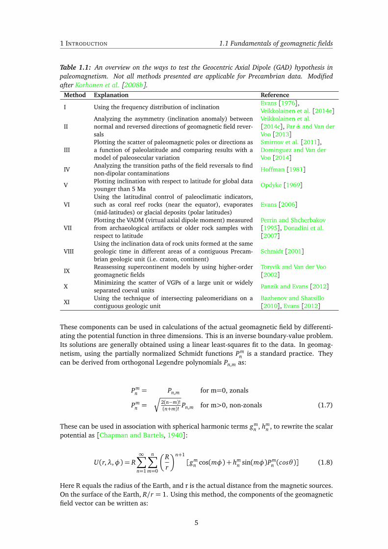
Table 1.1: An overview on the ways to test the Geocentric Axial Dipole (GAD) hypothesis inpaleomagnetism. Not all methods presented are applicable for Precambrian data. Modifiedafter Korhonen et al. [2008b].

Method Explanation Reference

I Using the frequency distribution of inclinationEvans [1976],Veikkolainen et al. [2014e]

IIAnalyzing the asymmetry (inclination anomaly) betweennormal and reversed directions of geomagnetic field rever-sals

Veikkolainen et al.[2014c], Parés and Van derVoo [2013]

IIIPlotting the scatter of paleomagnetic poles or directions asa function of paleolatitude and comparing results with amodel of paleosecular variation

Smirnov et al. [2011],Dominguez and Van derVoo [2014]

IVAnalyzing the transition paths of the field reversals to findnon-dipolar contaminations

Hoffman [1981]

VPlotting inclination with respect to latitude for global datayounger than 5 Ma

Opdyke [1969]

VIUsing the latitudinal control of paleoclimatic indicators,such as coral reef rocks (near the equator), evaporates(mid-latitudes) or glacial deposits (polar latitudes)

Evans [2006]

VIIPlotting the VADM (virtual axial dipole moment) measuredfrom archaeological artifacts or older rock samples withrespect to latitude

Perrin and Shcherbakov[1995], Donadini et al.[2007]

VIIIUsing the inclination data of rock units formed at the samegeologic time in different areas of a contiguous Precam-brian geologic unit (i.e. craton, continent)

Schmidt [2001]

IXReassessing supercontinent models by using higher-ordergeomagnetic fields

Torsvik and Van der Voo[2002]

XMinimizing the scatter of VGPs of a large unit or widelyseparated coeval units

Panzik and Evans [2012]

XIUsing the technique of intersecting paleomeridians on acontiguous geologic unit

Bazhenov and Shatsillo[2010], Evans [2012]

These components can be used in calculations of the actual geomagnetic field by differenti-ating the potential function in three dimensions. This is an inverse boundary-value problem.Its solutions are generally obtained using a linear least-squares fit to the data. In geomag-netism, using the partially normalized Schmidt functions Pm

n is a standard practice. Theycan be derived from orthogonal Legendre polynomials Pn,m as:

Pmn = Pn,m for m=0, zonals

Pmn =

q

2(n−m)!(n+m)! Pn,m for m>0, non-zonals (1.7)

These can be used in association with spherical harmonic terms gmn , hm

n , to rewrite the scalarpotential as [Chapman and Bartels, 1940]:

U(r,λ,φ) = R∞∑

n=1

n∑

m=0

�

R

r

�n+1

[gmn cos(mφ) + hm

n sin(mφ)Pmn (cosθ)] (1.8)

Here R equals the radius of the Earth, and r is the actual distance from the magnetic sources.On the surface of the Earth, R/r = 1. Using this method, the components of the geomagneticfield vector can be written as:

5


B(r) =nmax∑

n=1

n∑

m=0

−(n+ 1)�

R

r

�n+2

[gmn cos(mφ) + hm

n sin(mφ)]Pmn (cosθ)

B(θ) =nmax∑

n=1

n∑

m=0

�

R

r

�n+2

[gmn cos(mφ) + hm

n sin(mφ)]dPm

n (cosθ)dθ

B(φ) =nmax∑

n=1

n∑

m=0

m

sinθ

�

R

r

�n+2

[gmn sin(mφ)− hm

n cos(mφ)]Pmn (cosθ) (1.9)

This theory is analogous to the one-dimensional Fourier analysis and was originally pre-sented in 1839 by the German mathematician Carl Friedrich Gauss (1777-1855), who pub-lished a quantitative proof of Gilbert’s theory in Allgemeine Theorie des Erdmagnetismus.Gauss was able to calculate the four highest degrees of the field, which corresponds to24 = 16 poles. In his output, geomagnetic results were obtained at 84 points on the Earth’ssurface, as interpolated from three isomagnetic charts. These include Barlow’s declinationchart (isogonic chart), Horner’s inclination chart (isoclinic chart), and Sabine’s total intensitychart (isodynamic chart) [Merrill et al., 1998]. This approach can be seen as revolutionaryin terms of quantitative geomagnetism.

The functions used in Gauss’s technique are divided into zonal, sectorial and tesseral har-monics with n−m zero-points in the latitude limit −90◦ ≤ λ≤+90◦, as seen in Figure 1.1.Each of the terms can be regarded as an hypothetical individual source of the magnetic fieldlocated in the center of the planet rather than a real physical entity. Although the geomag-netic field is actually not produced in the center but in the outer core, models of this kindcan give a mathematically sound description of the field as observed on the Earth’s surface.Moreover, this also means that the sum of a geocentric dipole and a set of higher-degreemultipoles can give rise to a field similar to that caused by an offset dipole at an arbitrarydistance from the Earth’s center. The phenomenon, inherent to all potential field modelling,is called the non-uniqueness problem, and will be further discussed in Chapter 2. Higher-degree coefficients are attenuated more strongly with the distance from the source thanlow-degree ones, and for a long time, noise made it virtually impossible to observe anythingbeyond the 60th degree [Merrill et al., 1998]. Situation has improved fast, and results fromthe German CHAMP (Challenging Minisatellite Payload) satellite mission along with aero-magnetic and marine magnetic data have made it possible to construct a model up to the720th degree [Maus, 2008].

Spherical harmonic models are generally useful only if a statistically significant number ofuniformly distributed high-quality observations are available. Theoretically a decompositionof n:th degree requires at least n2 + 2n points of data, and the truncation of series canresult in negative side effects as predicted from Parseval’s theorem. In the era of magneticobservatories and sea-based measurements, the scarcity of data posed a problem, but afterthe advent of satellite surveys, e.g. NASA’s Magsat mission [Arkani-Hamed and Strangway,1986], situation has improved. If the criterion is not met, the geomagnetic field at a givensite can be modelled e.g. using a vectorial sum of local dipolar fields, as done in a study ofMartian crustal magnetism [Langlais et al., 2004]. Spherical cap harmonic models [Haines,1985] can be used for areas relatively close to the pole, with Finland as a good example[Nevanlinna et al., 1988].

6


High-resolution models of the present-day field, such as IGRF (International GeomagneticReference Field), generated and updated by International Association of Geomagnetism andAeronomy [IAGA, 2010] can include harmonics up to the 13th degree, which corresponds to213 = 8192 separate poles. Using higher-degree harmonics is more complicated, since thesewould be affected not only by the main geomagnetic field, but also by the crustal magneticanomalies. These can locally overshadow the main field, a phenomenon well visible e.g.below the 20× 40× 70 km large iron ore deposit of Kiruna, northern Sweden, where thehighest strengths of the field are even 400 µT [Korhonen, 1999].

The separation of the internal geomagnetic field into core-generated and crustal parts is veryclear since the solid material in the mantle of the Earth, except in the uppermost parts, is notcold enough for a permanent magnetism to survive, but not hot enough for being molten andgenerating a dynamo there [Merrill et al., 1998]. The fluid convection in the outer core, andpotentially also the stability of the internal field is strongly governed by the presence of thesolid inner core, currently with a radius of 1220 km but slowly growing due to the secularcooling which leads to the solidification of iron alloy on the outer core. For the most of thePrecambrian, perhaps until 1.5± 0.5 Ga, the core has been entirely liquid [Labrosse et al.,2001]. Time estimates of this kind can be higher or lower depending on whether the core hasa larger or smaller concentrations of radiogenic isotopes, most prominently potassium (40K)[Wessmann and Wood, 2002] but possibly also uranium (235U, 238U) and thorium (232Th).Unfortunately, the value is dependent on several poorly known geothermal parameters andan analytical solution is available only for the unreal situation where radioactive material isentirely absent from the core [Labrosse et al., 2001]. While 99 % of the magnetic energy isin outer and inner parts of the core altogether, the solid inner core contains roughly 10 % ofthis value [Glatzmaier and Roberts, 1996].

As derived from the latest IGRF model, harmonics for the first four degrees of the field areshown in Table 1.3, with nanoteslas [nT] as a unit. In the notation gm

n /hmn , n stands for the

degree and m for the order. Since the field is turning to the toroidal phase due to the rotationof the planet (α phenomenon) and back to the poloidal phase in the convection cells of theouter core (ω phenomenon), it can be divided in distinct symmetric and antisymmetric termsaccording to Table 1.4. For the antisymmetric terms (dipolar family), m+ n is odd, and forthe symmetric terms (quadrupolar family), m+ n is even. In spite of this representation, theactual field observed at the surface is entirely poloidal, since the toroidal field has no radialcomponent [McElhinny and McFadden, 2000]. The total number of Gauss coefficients gm

nand hm

n up to degree n can be obtained as follows:

n∑

n=0

gmn =

�

2(n+ 1)2

�

n=n2+ 3n

2n∑

n=0

hmn =

�

n+ 1

2

�

n (1.10)

For example, the number of gmn terms is 9 and the number of hm

n terms required is 6, whenn≤ 3 (see also Table 1.4). Accordingly, the variance of the field as a function of the harmonicdegree, also referred to as power spectrum, was formulated by Lowes [1966]:

B2n = (n+ 1)

n∑

m=0

�

(gmn )

2+ (hmn )

2�

(1.11)

7


Zonal harmonicsG(3,0)

Sectorial harmonicsG(6,6)

Tesseral harmonicsG(6,3)

Figure 1.1: Examples of the spherical harmonic decomposition of the geomagnetic field. Areaswith positive values are shown with red and those with negative values are blue. Three typesof functions exist: 1) Zonal functions, which depend only on latitude, 2) Sectorial functions,which depend both on latitude and longitude, though their sign is only dependent on longitude,3) Tesseral functions, in which values and signs change regularly with respect to latitude andlongitude, forming a chessboard-style pattern.

Using Equation 1.11, it is possible to compare relative strengths of different-degree fields.However, this can only be done on the surface of the Earth, since m= 0.

The boundary between the Earth’s mantle and the liquid outer core is regarded as the upperlimit of the magnetic source area in most geomagnetic calculations. Seismic velocity datacan be used for the validation of the result, currently ca. 3500 km from the Earth’s center.In case of IGRF, it is a standard procedure to calculate a model before its respective epoch,so the latest coefficients for the field strength and secular variation must be considered ap-proximate. It has been known for a long time that higher-degree terms of the field changemore rapidly than lower-degree ones. Constable and Parker [1988] proposed that the vari-ance σ of Gauss coefficients of a distinct degree n as a function of time follows the normaldistribution, if the axial dipole is neglected:

σ2n =

(c/R)2nα2

(n+ 1)(2n+ 1)(1.12)

Here c is the radius of the core, R is the radius of the Earth, and α a constant dependingon the strength of the field [nT]. In practice, the terms small and distant enough are oftenreduced to zero, since the potential of the field decays with respect to r−2 and the mag-netic field strength according to r−3. At a given distance r, the resolution of a sphericalharmonic model (ρ) can be evaluated using the semiwavelength formula (Equation 1.13),and solutions can be seen in Table 1.2, with r = 6378 km (the Earth’s radius).

ρ =πr

n−m(1.13)

8


Table 1.2: Spherical harmonic semiwavelengths.n-m Semiwavelength10 2000 km20 1000 km60 330 km

100 200 km

Modelling features with a large geographic extent requires low-degree harmonics and theircontribution is not restricted to a certain region but they affect the field globally and maycause a contradiction between the model and observations elsewhere. For instance, it isnot easy to include the large Siberian anomaly in the models. This feature, which may beindication of the future position of the geomagnetic north pole, is well visible in geomagneticfield maps and has a noticeable influence also on the field directions observed in Finland[Pesonen et al., 1994].

The observation that the geomagnetic field can change its polarity is a direct consequenceof Maxwell’s equations, but the first discoveries of the geomagnetic polarity opposite to thepresent one were made not much more than a century ago [David, 1904, Brunhes, 1906].The reversal of the field is a physically complex phenomenon, not just a collapse of the maindynamo field and its 180◦ directional change. This also means that the terms reversal andtransition have different meanings. Transition is most often referred to as the rapid changeof the magnetic field vector in the middle of the reversal, though it has also been statedthat the whole division between transitional and stable directions is incorrect [Harrison,1995]. As non-dipolar contributions to the field can be locally strong, the time-averagednormal and reversed directions may significantly deviate from the antiparallelism, notablyin cases where the non-dipolar part maintains its polarity while the dipole field undergoesa polarity change. Following Nevanlinna and Pesonen [1983] and applying the definitionb0

n = (n+ 1)(g0n) [Lowes, 1974], the ratio of non-dipolar and dipolar (ND/D) components

of the field can be calculated as:

N D/D =

s

∞∑

n=2

(b0n)

2

(b01)

2(1.14)

The time needed for a complete reversal varies from a few thousand up to 28 000 years, withan average of 7000 years [Clement, 2004], and decay in intensity can be typically observedbefore sudden directional changes occur. The last reversal of the field, called the Brunhes-Matuyama reversal, occurred 0.78 Ma ago and lasted no more than 12 000 years [Singer andPringle, 1996]. Models, such as the Parker-Levy dynamo [Hoffman, 1977, Gibbons, 1998],have been used to simulate the observed phenomenon that the field prior to the reversal isdegenerated more slowly at polar latitudes than in the vicinity of the equator. It has beendisputed whether the reversal frequency obeys the Poisson distribution or not, i.e. whetherreversals, or more precisely the lengths of polarity intervals, are temporally independent ofeach other [Constable, 2000] or not [Loper and McCartney, 1986]. According to Gubbins[1999], the concept of a stable polarity period between reversals is misleading, since be-tween two successful reversals, there are on average 10 excursions, which are unsuccessfulattempts of the field to change polarity. In the current Brunhes chron, five excursions havebeen confirmed, the Laschamp (40 ka ago) and Blake (120 ka ago) being the most obviousones [Channell, 2006].

9


Table 1.3: The magnitudes of spherical harmonics of first four degrees in IGRF-2015 model[IAGA, 2010] in nanoteslas [nT]. For zonal quadrupole, octupole, and hexadecapole, the non-dipole to dipole ratio (ND/D, Equation 1.14) is also given.

Name n m g h ND/D (zonals only)

dipole1 0 -29439.5 01 1 -1502.4 4801.1

quadrupole2 0 -2453.1 0 8.3 %2 1 3006.5 -2822.72 2 1682.1 -639.9

octupole

3 0 1346.2 0 4.6 %3 1 -2345.8 -117.53 2 1217.2 237.23 3 593.7 -547.3

hexadecapole

4 0 905.6 0 3.1 %4 1 819.0 288.44 2 122.1 -195.24 3 -335.1 182.44 4 78.2 -313.2

Table 1.4: Antisymmetric (odd) terms, i.e. dipole family, and symmetric (even) terms, i.e.quadrupole family, of the geomagnetic field up to the third degree.

Field Antisymmetric terms Symmetric termsdipole g0

1 g11 h1

1quadrupole g1

2 , h12 g0

2 , g22 , h2

2octupole g0

3 , g23 , h2

3 g13 , g3

3 , h13, h3

3

Table 1.5: Magnetostratigraphic units and the corresponding geochronologic time division.After McElhinny and McFadden [2000] with modifications.

Magnetostratigraphic unit Geochronologic unit Duration (Ma)Polarity megazone Megachron 100− 1000Polarity superzone Superchron 10− 100Polarity zone Chron 1− 10Polarity subzone Subchron < 1Polarity cryptozone Cryptochron < 0.03

The proof of the continuous record of the past reversals of the geomagnetic field stored in theoceanic crust was crucial to the sea-floor spreading hypothesis [Vine and Matthews, 1963],which states that rocks near the mid-oceanic ridge are generally younger than those closerto the continental shelf. The best-known example is the Atlantic Ocean, where the spreadingrate has slowed down from the late Cretaceous value (30 km/Ma) to the present one (16km/Ma) [Ogg and Smith, 2004]. Studying the reversal sequences, whether observed in theocean floor or in continental lithosphere, is referred to as magnetostratigraphy, and one ofits long-lived problems regards the comparison of reversal records from different parts ofthe world. These give an unique polarity interval timescale, unlike the commonly used bio-and lithostratigraphic methods. In the last 330 Ma, the vast majority of polarity intervals haslasted for less than 1 Ma, but on the other hand, the Cretaceous and Kiaman superchronsare the only intervals with lengths greater than 4 Ma [Opdyke and Channell, 1996].

Table 1.5 shows the scheme for magnetostratigraphic polarity units, along with their re-spective polarity chron (epoch) names. However, this division does not include very shortpolarity intervals, referred to as events, lasting no more than 105 years. Neither does it take

10

1 INTRODUCTION 1.2 Precambrian data and paleointensity

into account episodes with a small dipolar field strength, relatively strong higher-degreefields and low-latitude paleomagnetic poles without evidence of a successful field reversal.These are called excursions [Hoffman, 1981, Valet et al., 2008], and their presence hasgiven rise to theories that the reversals are the end members of the secular variation of thefield. In case of a non-oscillatory, mainly dipolar field this might be at least partly possible[Schmitt et al., 2001]. In analyses of secular variation, scientific interest is generally focusedon the stable-polarity field, and hence excursional directions are often filtered out using cut-off criteria, either variable [Vandamme, 1994] or constant [Johnson and Constable, 2008].However, transitional VGP paths, when viewed from coeval data collected from distant ar-eas, can provide an insight into the non-dipolar field since the dipolar field is diminishedduring the transition [Gubbins and Coe, 1993, Hoffman, 1981].

1.2 Precambrian data and paleointensity

During the last half a century, the paleomagnetic method has been successfully applied torocks with ages ranging from a few thousand up to a few billion years. In addition to dataon the field directions, results of the intensity of the field can be used, following the ideathat a set of small, so-called single-domain (SD) particles will be magnetized in relationto the prevailing electromagnetic field, when the temperature falls below a critical block-ing temperature. This principle is challenged by the multidomain (MD) behaviour, viscousremagnetization and changes in the physico-chemical composition of grains. The first andstill the most widely used method developed to overcome these factors was introduced byThellier and Thellier [1959], who used a double-heating technique to estimate the intensityof the magnetic field.

After several improvements, Thelliers’ method for paleointensity studies has been used topoint out that the average dipole moment has been much weaker during the last 300 Ma,when compared to the present-day value [Selkin and Tauxe, 2000]. There are also records ofpaleointensity from earlier times, but most of them have been measured from Archean andPaleoproterozoic North American rocks, with only a handful of results from other continents[Dunlop and Yu, 2004]. In a geocentric axial field, the values of paleointensity, as observedat a certain latitude λ, can be easily reduced to their equatorial values using Equation 1.15:

F = F0

p

1+ 3 sin2λ (1.15)

where F is the paleointensity obtained e.g. using the Thellier technique and λ can be es-timated from the dipole equation tan I = 2 tanλ, with I being the measured inclination ofthe ancient magnetization. Here F0 means the intensity at the equator, presently ca. 30 000nT [IAGA, 2010]. Obtaining intensities in non-zonal geocentric dipolar fields is possible viasimple rotation matrices, but for offset dipolar fields and any kinds of multipolar fields, thesituation may be far more complex. The behaviour of intensity in zonal, equatorial and tiltedgeocentric dipolar fields is illustrated in Figure 1.3, whereas Figure 1.4 shows intensity forthree different zonal fields. It is noteworthy how much more strongly a low-degree axialmultipole field can affect the intensity of the field, when compared with the influence it hason the inclination observed at different paleolatitudes (Figure 1.2).

11

1.2 Precambrian data and paleointensity 1 INTRODUCTION

90 60 30 0 30 60 90 ( )

20

10

0

10

20

d(I)

()

GAD = -30000 nT GAD = -30000 nT, G2 = 0.06

GAD = -30000 nT, G3 = 0.06GAD = -30000 nT, G2 = 0.06, G3 = 0.06

Figure 1.2: Inclination anomaly, i.e. the difference between the observed inclination valueat a given latitude, and the inclination expected from the GAD model, calculated as d(I) =I − I(GAD) [Cox, 1975] for superposition fields of GAD and zonal multipole fields. This quan-tity is roughly half of the inclination asymmetry parameter ∆(I), which is defined by Veikko-lainen et al. [2014c] as the great-circle distance between mean normal- and reversed-polaritydirections. Alternatively. the behaviour of inclination with respect to latitude can be studiedby calculating the difference of observed cumulative inclination distribution from that predictedby GAD Heimpel and Evans [2013]. For the influence of a small axial octupole field on theintensity at different paleolatitudes, see Figure 1.4.

Since it is evident that a small axial octupole can have a remarkable impact on the fieldintensity especially at equatorial and polar latitudes (Figure 1.4), plotting values of F withrespect to paleolatitude can be used to find possible zonal field coefficients higher thanGAD. Fitting observational inclination data with models has been most challenging whenthe Precambrian data have been concerned [Donadini, 2007, Dunlop and Yu, 2004], but ina study of 879 observations from the last 400 Ma, Perrin and Shcherbakov [1995] made amore successful attempt to point out that no statistically significant departure of the averagegeomagnetic field from the GAD has taken place. High scatter, however, makes this resultless reliable and therefore other methods for testing the GAD should be preferred instead ofthat. Not just experimental errors are to blame for this, but the geomagnetic field itself issubject to rapid changes [Holme and De Viron, 2005, Yang et al., 2000].

The geographic distribution of Precambrian data is more restricted than that of youngerentries, since no marine data are available, and in continental areas, only the most stableshield and platform areas are points of interest. As the Finnish bedrock is among the oldestin Europe, including rocks as old as 3.5 billion years [Mutanen and Huhma, 2003], a longtradition of studying the Precambrian has emerged in Finland. In geological terms, most ofthe Finnish rocks belong to the Archean craton of Karelia and the Proterozoic Svecofennianorogen inside the continent of Baltica, one of the nearly 30 confirmed Precambrian conti-nents. The definition of a continent here does not strictly follow the conventional view of

12

1 INTRODUCTION 1.2 Precambrian data and paleointensity

GAD, G(1,0) Equatorial, G(1,1)

Equatorial, H(1,1) Tilted, G(1,0)+G(1,1)+H(1,1)

30000

34500

39000

43500

48000

52500

57000

Figure 1.3: Intensity in different kinds of dipolar fields. Helsinki 60◦N, 25◦E is situated inthe center of each subplot. The minimum of the field intensity (obtained at the geomagneticequator) is 30000 nT and the maximum (obtained at geomagnetic poles) is 60000 nT.

a large, unitary landmass, since there are also microcontinents, such as Madagascar [Meertet al., 2003a] and Seychelles [Torsvik et al., 2001] with granitic rock outcrops and maficdykes. There are also geological units, which lie presently far from one another, but wereunited in the past. Examples of these include the Grunehogna craton, now belonging toAntarctica, but a part of Kalahari craton ca. 1.1 Ga ago [Jones et al., 2003] and the trans-Atlantic Congo - São Francisco craton [D’Agrella-Filho et al., 2004]. Conversely, certaincratons, such as Slave and Superior in North America, drifted independently before theirunification [Whitmeyer and Karlstrom, 2007]

Paleomagnetic information, either Precambrian or from younger eras, is stored in the nat-ural remanent magnetization (NRM) vector of rocks. In addition to radioactive decay, thisis the second geophysical quantity with a geological memory. NRM, also called remanence,is a property of magnetism-carrying minerals of the rock, such as magnetite, hematite andpyrrhotite. It is only present in different types of ferromagnetic minerals, not in param-agnetic or diamagnetic ones, which are much more common in the bedrock and carry theinduced magnetization only. In ferromagnetic material, the magnetization (so-called ther-moremanent magnetization, TRM) is locked when the temperature falls below the charac-teristic Curie temperature, and on the other hand, it will disappear permanently if the rock is

13

1.2 Precambrian data and paleointensity 1 INTRODUCTION

9060300306090 ( )

30000

35000

40000

45000

50000

55000

60000

65000

70000

|F| (

nT)

= 30000 nT

Multipole model ( = 30000 nT, = 0, = 1800 nT)

Multipole model ( = 30000 nT, = 0, = 1800 nT)

Figure 1.4: Absolute value of geomagnetic field intensity (|F|) in a pure geocentric axial dipolefield and in two zonal multipole fields. The intensity of g0

1 at the geographic equator is -30000nT in each case. If the axial octupole g0

3 is of the same sign as g01 (negative in this case), the

intensity is strengthened at the poles and weakened at the equator. However, with g01 and g0

3being of different signs, the field becomes weaker at poles and stronger at the equator.

reheated. In slowly cooled plutonic rocks, such as granites, the acquisition of magnetizationmay take such a long time that the mineral composition of the rock is subject to a significantchange, and in these cases, the developing magnetization is referred to as thermochemicalmagnetization (TCRM). Rapidly cooled rocks, e.g. successive lava flows, are more likely tomaintain their original mineral composition and their summarized eruption time is close tothe average secular variation timescale, roughly 103 to 105 years [Tanaka et al., 1995, Lajet al., 1999, Smirnov et al., 2011].

Among the most interesting features in the Precambrian bedrock are mafic dyke swarms(e.g. Green et al. [1987], Buchan and Halls [1990]), since they are easy to discover andsample, can be dated radiometrically, and their record of the paleomagnetic field is in manycases well preserved. The survival of a permanent remanence is most likely if it is nearlyequal to or larger than the induced one. This can be evaluated, if the NRM, the volumesusceptibility χv (10−6 in SI units), vacuum permeability µ0 (4π × 10−7T mA−1) and the

14

1 INTRODUCTION 1.3 Paleomagnetic poles

present geomagnetic field strength B are known. The relation is called Q, or Königsbergerratio:

Q =µ0(NRM)

Bχv(1.16)

One must bear in mind here that the Q value calculated via 1.16 is a present-day estimateand the original Q can be different e.g. due to the decaying of the original NRM in time.The primary origin of the observed NRM can be evaluated in a number of stability tests.In a fold test, a pre-folding remanence is characterized by scattered directions on two dif-ferent sides of the fold, which however converge after the structural correction. In case ofpost-folding (secondary) remanence, the structural correction, on the contrary, increases thescatter. Whenever conglomerates are present, a conglomerate test should reveal randomdirections (primary remanence) or nonrandom ones (secondary remanence). By comparingthe remanence locked in igneous bodies (notably dykes) with that in baked and unbakedhost rocks, a baked contact test [Everitt and Clegg, 1962] can be made. The reversal testis based on the antiparallelism of normal and reversed directions in case of a GAD field. Ifthese directions are non-antipodal, they may hint to secondary components of remanence,apparent polar wander during the reversal or non-GAD fields [Pesonen and Nevanlinna,1981, Veikkolainen et al., 2014c].

Secondary sources of magnetization are most obvious in cases where the magnetizationof the sample is statistically indistinguishable from the present field components, and thecorresponding Q values are low. However, sites located higher than their surroundings areprone to lighning-induced remagnetization (LIRM) which generally leads to very high Qvalues (Q > 50). This is often detected from archeological sites [Jones and Maki, 2005], butsometimes visible even in Precambrian rocks, such as those of the South African Vredefortimpact structure [Carporzen et al., 2012, Salminen et al., 2013].

1.3 Paleomagnetic poles

The paleomagnetic data of the Precambrian are mostly directional, i.e. it is described bythe declination (D) and inclination (I) of ChRM. For working with these observations, theconcept of paleomagnetic pole was introduced by Creer et al. [1954]. This is the north orsouth pole of the geomagnetic field that corresponds to the observed direction of the field ata fixed location at a fixed point in history. This theory presumes that the field is describedby GAD only, so simple spherical trigonometric formulae are valid. Poles calculated as suchare referred to as virtual geomagnetic poles (VGPs). The accurate determination of a VGPrequires that the primary remanence of the studied rock has been properly isolated. Sec-ondary components of magnetization, such as chemical remanent magnetization (CRM) orviscous remanent magnetization (VRM) must be removed using alternating magnetic field(AF), thermal or chemical demagnetization. This procedure is typically done after prelimi-nary petrophysical measurements, which give information about the density and magneticmineralogy of the samples.

Curie temperature determinations yield more detailed information on magnetic carriers andtheir grain size as well as domain type are determined by hysteresis curves. The most com-mon domain types are single domain (SD), multidomain (MD) and pseudo-single domain

15

1.3 Paleomagnetic poles 1 INTRODUCTION

(PSD). Some rocks have more than one magnetic carrier mineral, but these can be dis-tinguished based on their Curie temperatures. Most often these minerals lie within theFeO − TiO2 − Fe2O3 ternary system, so they contain various contents of iron, oxygen andtitanium [McElhinny and McFadden, 2000].

In the Solid Earth Geophysics research laboratory of the University of Helsinki, most sampleshave been demagnetized using three-axis AF demagnetization equipment, part of the SQUID(Superconducting Quantum Interference Device). This kind of equipment is very sensitiveand therefore useful for studying magnetically very weak samples. The procedure is doneby increasing the alternating magnetic field step by step, up to 160 mT , until the finalvalues for declination, inclination and intensity are obtained. The characteristic remanentmagnetization (ChRM) is obtained using special vector treatments of the demagnetizationdata, either by principal component analysis or by so-called "line find" method. It should, inideal case, be a reliable record of the ancient geomagnetic field. Using the paleomagneticdirection (Dm, Im) and the latitude and longitude of the sampling site, the latitude of thepaleomagnetic pole (λp) can be calculated, with θ as magnetic colatitude (the great-circledistance from site to the pole) [Merrill et al., 1998]:

λp = arcsin(sinλs cosθ + cosλs sinθ cos Dm) (1.17)

cotθ =1

2tan Im (1.18)

Here the conditions −90◦ ≤ λp ≤ 90◦ and λ = 90◦ − θ are satisfied. Assuming −90◦ ≤ β ≤90◦, the equation of β can be applied to calculate the longitude of the paleomagnetic pole(φp) as follows:

β = arcsin

�

sinθ sin Dm

cosλp

�

(1.19)

φp =

¨

φs + β if cosθ ≥ sinλs sinλpφs + 180◦− β if cosθ < sinλs sinλp

(1.20)

The equations can be used both ways, and hence it is also possible to calculate the paleo-magnetic direction from its corresponding VGP via iteration, if the sampling site is known.Moreover, if the sampling site coordinates (λs, φs) are unknown, they can be solved via thedirection (Dm, Im) and the pole (λp, φp) [Veikkolainen et al., 2014b].

Because of the possibility of two equally likely directions of the geomagnetic field, eithernormal (N) or reversed (R), two solutions for a paleomagnetic pole always exist. In anaxially symmetric field, declination is zero everywhere, so the paleolongitude of the sam-ple cannot be obtained via the concept of paleomagnetic poles, which inherently assumesGAD to be valid. However, solutions for the determination of the absolute paleolongitudehave been presented using e.g. hotspot tracks in the Phanerozoic [Smirnov and Tarduno,2010, Doubrovine et al., 2012] or recently, using combined geophysical and kimberlite oc-currence data [Torsvik et al., 2010]. Even the determination of paleolatitude is prone to the

16

1 INTRODUCTION 1.3 Paleomagnetic poles

hemispherical ambiguity since absolute polarities are not known for the Precambrian, ex-cept perhaps for Laurentia and Baltica in the Mesoproterozoic [Bingen et al., 2002, Pesonenet al., 2012b]. Observations show that paleomagnetic poles of nearly same age fall close toone another even if they originate from different parts of the same continent [Irving, 1964].This has given justification for the theory that a geocentric dipole accounts for most of thegeomagnetic field, but it alone does not prove that the dipole is axial. At least theoreti-cally, this problem can be solved using climatically sensitive sediments [Irving, 1964, Evans,2006]. The farther one goes to history, the less does one generally get trustworthy informa-tion about the character of the field, since the number of reliable paleomagnetic poles fallssignificantly with age [Van der Voo, 1993].

The determination of an accurate and precise paleomagnetic pole typically requires a lot ofrepeated measurements of rocks from the same geologic unit. These can be spot readings, ormore preferably obtained from a continuous time series, such as a dyke swarm, lava flow orsedimentary strata. In all cases, statistical treatment of data is mandatory, since the scatter ofindividual VGPs is typically large. Their distribution of points on a sphere can be estimatedusing a Fisherian probability density function:

PdA(θ) =κ

4π sinκeκ cosΘ (1.21)

where dA is the area differential, κ is the concentration parameter, and Θ is the angle be-tween the directions of a single sample and the averaged set of samples [Fisher, 1953]. Fordirections, the mean vector is characterized by the radius of the 95% cone of confidence, andfor the mean paleomagnetic pole, the corresponding quantity A95 is applied. If continentaldrift has shifted the location of the sampling site after the acquisition of the magnetization,paleomagnetic poles deviate from the present geographic pole to a varying extent with re-spect to age. Hence for separate poles of varying ages on a same continent, or preferablyon a same craton, an apparent polar wander path (APWP) can be determined. This con-cept, introduced by Creer et al. [1954], is very convenient if a number of observations withwell-defined ages and small statistical errors exists.

In 1970s it was observed that data from reversed directions tends to yield poles farther fromthe sampling site, than normal data does. These are called far-sided and near-sided effects,and can be explained e.g. by a assuming the field to be slightly axially offset as a whole orto have a small offset dipole in addition to the dominating geocentric one [Wilson, 1972,Nevanlinna and Pesonen, 1983]. For Precambrian observations, it is generally impossible todetermine absolute polarities, but a possible asymmetry in pole positions is still visible, suchas in the Lake Superior region [Pesonen, 1979, Tauxe and Kodama, 2009]. In case thereis poor knowledge of the geomagnetic field that generated the observed paleomagnetic di-rections, Fisherian statistics must be used with caution. Because Equation 1.21 describesthe precision, not the accuracy of the measurements, systematically erroneous data can infact have a very small A95 confidence circle. This kind of error may be caused e.g. by anoffset dipole or by a zonal non-dipolar field [Pesonen and Nevanlinna, 1981]. As expectedfrom paleosecular variation, the dispersion of poles should actually be dependent on lati-tude, growing from the equator towards the poles. If the poles are very tightly clusteredat a given paleolatitude, it may reflect the inadequately averaged secular variation. On theother hand, effects such as tectonic alteration can cause abnormally high scatter in the data[Butler, 1992].

17

1.4 The PALEOMAGIA database and outline of research 1 INTRODUCTION

The equations used for calculating paleomagnetic poles inherently assume that the GAD hy-pothesis is valid. This requires that the remanent magnetization has been acquired duringan interval long enough to average out secular variation. Since the motion of the poles isseen from the present-day frame of reference, the resulting APW curve describes the motionof the continent rather than that of the pole. For example the APWP of Laurentia between1150-1000 Ma is shown in Figure 1.5. Although error limits of different-aged poles over-lap substantially, the majority of younger poles is closer to the equator than older poles,thus giving implications for the rapid drift of North America especially during 1111-1103Ma [Swanson-Hysell et al., 2009] rather than any pervasive offset dipole or non-dipolareffects as previously suggested by Nevanlinna and Pesonen [1983]. For reconstructions ofcontinents, using APWPs is not a necessity, since individual high-quality poles from severalcratons can alternatively been used, following Buchan et al. [2000], Buchan [2013] andPesonen et al. [2003].

1.4 The PALEOMAGIA database and outline of research

The prerequisite for the research described in this thesis, and statistical paleomagnetic anal-ysis in general, is the presence of an abundant and up-to-date database of paleomagneticresults of the period to be studied. Examples of the widely used databases include the GE-OMAGIA50 database, with 3798 paleomagnetic and archeomagnetic results from the last50 000 years [Korhonen et al., 2008a], and the Magnetics Information Consortium (MagIC)database [Jarboe et al., 2012]. For a long time, no comprehensive catalogue for the entirePrecambrian was in existence, although smaller data compilations had been made e.g. inNorth America and Australia [Irving et al., 1976, McElhinny and Cowley, 1977] and also inthe former USSR [Khramov, 1971, 1979]. In Fennoscandia, the lack of a proper catalogueled to conflicting paleogeographic models for the same area [Poorter, 1981, Pesonen andNeuvonen, 1981, Piper, 1982]. Hence a growing demand for a proper catalogue emerged,and the first results of the paleomagnetic compilation of Baltica, including results from Ter-tiary down to Archean, were published in 1986 in the second EGT (European GeotraverseProject) Study Centre held in Espoo, Finland [Pesonen, 1987].

As the problems in paleomagnetism are mostly global and not restricted to a certain craton,the database project was to face a major improvement after the decisions made at the 4thNordic palaeomagnetic workshop [Abrahamsen et al., 2001]. The entries were convertedfrom text files into Excel spreadsheet format, and the collaboration between the University ofHelsinki and Yale University was to begin in 2001. The aim was to gather all Precambrian pa-leomagnetic directions and poles in a coherent way, preferring observations from original re-view articles and supplementing it with catalogue data, results from national survey reports,Ph.D. theses, etc. Finally, the data were transferred to an Apache server in 2013. The currentdatabase, called PALEOMAGIA (Paleomagnetic Information Archive), runs the PHP/MYSQLtechnology and can be accessed online at http://h175.it.helsinki.fi/database. Asof August 2014, the database comprises 2076 entries of igneous rock data, 1033 entries ofsedimentary data and 213 entries of metamorphic rock data, resulting in 3322 observations(entries) altogether.

1.4.1 Motivation and construction

The previous paleomagnetic databases, although widely used and well serving the paleomag-netic community, are incomplete in many ways. The most prominent shortcomings include

18

http://h175.it.helsinki.fi/database

1 INTRODUCTION 1.4 The PALEOMAGIA database and outline of research

Figure 1.5: Paleomagnetic poles of Laurentia in the late Mesoproterozoic delineating the west-ern arm of the so-called Logan Loop (1141-1050 Ma). Pole positions and their respective 95% limits of confidence are plotted according to their polarities, with red symbols for normalpolarity (N=32) and yellow symbols (N=25) for reversed polarity. Some well-defined poles arereferred with following abbreviations: J = Jacobsville Sandstone [Roy and Robertson, 1978],L/U M = Lower/Upper Mamainse Point Lavas [Swanson-Hysell et al., 2009], C = ColdwellComplex [Lewchuk and Symons, 1990], T = Thunder Bay Dykes [Pesonen, 1979], A = AbitibiDykes [Ernst and Buchan, 1993]. Mean normal and reversed poles for Central Arizona dia-bases (AZ, purple) [Donadini et al., 2009, 2012] are also shown. All observations satisfy theMV ≥ 3 (Modified Van der Voo) criterion [Van der Voo, 1993, Veikkolainen et al., 2014e].Diamond symbols point to the current locations of Lake Superior (LS, λS = 48◦, φS = 271◦)and Arizona (AZ, λA = 34◦, φA = 249◦). The grey shading shows the schematic way of themean APWP of Laurentia at 1120-1050 Ma.

19


the lack of a well defined reliability scale and latest geochronologic information. For ex-ample, the Global Paleomagnetic Database (GPMDB), available at the website of the Norwe-gian Geological Survey (http://www.ngu.no/geodynamics/gpmdb/), suffers from thesedrawbacks. In addition, the majority of its output is accessible to the user only as plain textfiles rather than organized tables.

The database presented here has been divided into separate tables for continents, conti-nental fragments and cratons. In some continents, most notably in the largest ones, thesubdivision into cratonic terranes and orogenies has also been made, e.g. the post-1830 MaLaurentia contains data from Arizona, Ellesmere, Grenville, Hearne, Mackenzie Mountains,Nain, Rae, Slave, Superior, Trans-Hudson and Wyoming, which previously drifted separately[Whitmeyer and Karlstrom, 2007]. Even though most continents are represented adequatelyenough in terms of the amount of data, concentrations are visible in Fennoscandia, CanadianShield and southern parts of Africa, as seen in Figure 1.7. Using a geostatistical binning pro-cedure to overcome the problem of unevenly distributed observations has been suggestedKent and Smethurst [1998], but can be seriously misleading if done using a simple latitudegrid without taking the cratonic division and the true spherical geometry of the globe intoaccount [Veikkolainen et al., 2014e,a].

For estimating the credibility of paleomagnetic data, the previously used Briden-Duff grad-ing, with a scale from A to D [Briden and Duff, 1981], has been replaced with the six-classmodified Voo grading (MV) [Veikkolainen et al., 2014e] in PALEOMAGIA. Unlike in the orig-inal grading of Van der Voo [1993], the resemblance to paleomagnetic poles of younger agehas not been considered here since Precambrian APWPs often contain self-closing loops withdifferent-aged paleomagnetic poles overlapping with 95% confidence level, and on the otherhand, most Precambrian continents lack complete Phanerozoic APWPs, which would be re-quired to effectively apply the seventh class of the original Van der Voo grading. Overlap ofpoles is also caused by repetitive paleomagnetic studies performed on same rocks. There-fore, rigorous filtering of the data evidently alleviates the construction of APWPs especiallyif the poles have precise age information, as several poles in the Late Precambrian LoganLoop [DuBois, 1962, Palmer, 1970, Pesonen, 1979] of North America do (Figure 1.5). Us-ing poles with MV ≤ 3 in APWPs or paleogeographic reconstructions should generally beavoided, and to ensure the validity of the model, comparison with geologically derived re-constructions (e.g. [Zhao et al., 2004, Johansson, 2009]) may be necessary. In Table 1.6,the distribution of the data into different MV quality grades is shown.

Although there is no doubt of successive geomagnetic field reversals in the Precambrian,large temporal gaps in APWPs render the concept of absolute polarity unusable. Separationto "N" and "R" polarities within a rock unit in different continents, however, is applied inthis database, unlike in GPMDB. The quotation marks in these notations simply inform thatdivisions to N and R are best estimates with presently available data, and one must bearin mind that "N" and "R" of one continent do not necessarily correlate with "N" or "R" ofanother one. A reasonably good match, however, can be obtained for Laurentia and Baltica,which most likely drifted together for the most of the Proterozoic as denoted by their APWPs[Pesonen et al., 2003] and paleolatitudes (Figure 1.10). Results, which cannot be correlatedwith any polarity pattern, or have both N and R directions present without a well-definedfield reversal, are most common in sedimentary data and are referred to as mixed-polarityentries (M) throughout the database.

The presence of dual-polarity entries indicates field reversals which can be effectively usedto evaluate the validity of the GAD hypothesis [Hospers, 1954] in the Precambrian, using the

20

http://www.ngu.no/geodynamics/gpmdb/


Table 1.6: Classification of PALEOMAGIA data entries (N=3322) according to their reliability.Grade Count of entries

MV = 6 103 (3.1 %)MV = 5 333 (10.0 %)MV = 4 607 (18.3 %)MV = 3 872 (26.2 %)MV = 2 893 (26.9 %)MV = 1 470 (14.1 %)MV = 0 44 (1.3 %)

asymmetry between normal and reversed directions [Veikkolainen et al., 2014c] as discussedin Chapter 3. A more commonly applied way of doing the testing is based on the inclinationfrequency analysis of Evans [1976], and this can also be used to produce cumulative distri-butions [Bloxham, 2000, Tauxe and Kodama, 2009, Heimpel and Evans, 2013]. Figure 2.1shows an example of applying the cumulative inclination method to moderate-to-high qual-ity igneous rock data in the database, with two theoretical distributions for comparison.Using inclination data for searching the most suitable combination of zonal geomagneticfields in the Precambrian is an integral part of this thesis [Veikkolainen et al., 2014e] anddiscussed more thorougly in Chapter 2. An alternative way to analyze the contribution ofnon-dipole field to the observed field follows paleosecular variation analysis, where the scat-ter of VGPs is typically plotted against paleolatitude. Figure 1.9 illustrates how this methodis applied to 0.5-2.9 Ga data from PALEOMAGIA and how the results can be compared withparametric geomagnetic field models for the last 5 Ma, 1.0-2.2 Ga and 2.2-3.0 Ga [Smirnovet al., 2011].

1.4.2 Structure of the database

The PALEOMAGIA database has been developed as a PHP/MYSQL based web applicationto allow users to access a wealth of paleomagnetic information in an easily understandableand user-friendly manner. In addition to GPMDB, original research articles, monographs,conference proceedings and other publications have been valuable sources of data, especiallyfor the last decade (years 2004-2013) which is represented by as many as 725 entries inPALEOMAGIA. Results from GPMDB have been in most cases included in PALEOMAGIA assuch, and also referred to by their respective GPMDB entry numbers. Additional remarkson different aspects, such as recalculation of poles due to errors in the original paper, orupdated age information, have been written in the comment column of database tables.Unlike GPMDB, PALEOMAGIA provides a comprehensive and conveniently accessible onlinedocumentation, where the contents available to its user are thoroughly explained.

The hierarchy of the finalized database is based on separate database tables, one or moreof which can be selected in the dynamically created query form. The user may also applyvarious search options, such as including peer-reviewed data only, sorting the data usingdifferent criteria, and setting requirements for the rock types, ages of magnetization and thequality of data. Free text queries based on the rock unit, terrane, authors or the publicationname are also possible. To optimize the structure of the database, not all data columnsvisible in the user interface exist in the database directly, but some of them are generateddynamically using server-side PHP scripts if they are directly dependent on one or more ofthe database column values via a simple mathematical equation. For example, paleolatitudeλ is related to inclination I in the GAD field via tan I = 2 tanλ, so whenever the inclination

21


Figure 1.6: A schematic view on how the data from various sources have been used to constructthe database used in this study. In the thumbnail in the upper right corner, David A.D. Evansand Lauri J. Pesonen are working with the data. [Pesonen et al., 2012].

values are stored in the database, there is no need to store the respective paleolatitude valuesas such. A schematic view on how the data from various sources has been fed in is illustratedby Figure 1.6.

1.4.3 Applying the data to study the evolution of the geomagnetic field

Due to its versatility, the PALEOMAGIA database can be used for a number of paleomagneticapplications, including tests of the GAD hypothesis throughout the Precambrian. For thispurpose, three out of nine methods described in Table 1.1 (Methods I, II and III) are appliedin this dissertation. In Chapter 2, the inclination frequency analysis [Evans, 1976] is em-ployed and the results by Veikkolainen et al. [2014e] are summarized. This approach waspreviously applied in a M.Sc. thesis [Veikkolainen, 2010], giving results closer to GAD thanseen in other studies. However, those preliminary results must be observed with caution,since the database was under construction at that point. Information on the geologic ages,and even cratons of its entries was in some cases missing or incomplete, so it was difficultto do the spatiotemporal binning in a geologically correct way as explained by Veikkolainenet al. [2014a]. Hence the inclination analysis was redone using the newest version of thedatabase [Veikkolainen et al., 2014b].

Estimating the functionality of the GAD model can be alternatively done by analyzing of thepolarity changes of the geomagnetic field. For this purpose, a compilation of the reversalsof the Precambrian was made and the parameters necessary for the determination of theasymmetries of polarity were calculated. These results were published by Veikkolainen et al.[2014c] and a brief summary of them is given in Chapter 3. In the final chapter, results from

22


70°S

50°S

30°S

10°S

10°N

30°N

50°N

70°N

W 90° 0° 90° E

Figure 1.7: Global distribution of observations in the PALEOMAGIA database. Only data withMV > 2 accepted. Larger symbols denote for higher quality. Blue symbols stand for results withMV ≥ 5.

23


0 10 20 30 40 50 60 70 80 90|I| ( ◦ )

0

20

40

60

80

100

Cum

ulat

ive

frequ

ency

(%)

Model 1. GADModel 2. GAD + G3 (0.20)Difference of Models 1 and 2Model 3. GAD + G2 (0.20)

Difference of Models 3 and 1Observed distribution (N=904)Difference of observed and GAD

Figure 1.8: Cumulative inclination distributions of GAD alone (Model 1), GAD with a negativeoctupolar field (Model 2), GAD with a positive quadrupolar field (Model 3) and the observedPrecambrian distribution. Entries from igneous rocks with MV ≥ 3 included, other entriesexcluded from the analysis. Difference curves of Models 2 and 1 as well as those of Models 3 and1 are also shown, along with the difference of the observed distribution and GAD. This methodis a modification of the traditional inclination frequency method, which is discussed further byVeikkolainen et al. [2014e] (Chapter 2) and Heimpel and Evans [2013].

24


0 30 60|λ| ( ◦ )

0

5

10

15

20

25

30

S b

y po

les

S for Precambrian data (N=55)Model G for 1.0-2.2 Ga (N=14)Model G for 2.2-3.0 Ga (N=9)

TAFI fit for 0-5 MaModel to observations (N=55)

Figure 1.9: The observed dispersion of virtual geomagnetic poles (S parameter) versus theabsolute value of paleolatitude (|λ|) is a commonly applied measure of paleosecular variationin recent eras and Precambrian alike. However, to obtain the true scatter between sites, alleffects of the within-site scatter (SW ) need to be removed [Biggin et al., 2008], yielding SB. Inthis example, 55 high-quality entries from PALEOMAGIA are accompanied by their error limitscorresponding to 2σ (two standard deviations from the mean) and the best statistical fit alongwith its error envelope. Parametric PSV models of S for timeslots of 0-5 Ma (TAFI fit; b = 0.25;a= 13.24), 1.0-2.2 Ga (b= 0.21; a= 11.10) and 2.2-3.0 Ga (b= 0.22; a= 7.56) by Smirnovet al. [2011] are also visible.

25


1000 1250 1500 1750 2000 2250 2500age (Ma)

−60

−40

−20

0

20

40

60

80

(∘ )

�� /��

Figure 1.10: Paleolatitudes of the Fennoscandian Shield (Baltica) and the Superior craton ofLaurentia between 2500-1000 Ma. Data from Baltica (red symbols) and those of Superior(cyan dots) have been filtered applying the MV ≥ 3 criterion. As a result, 111 entries fromBaltica and 255 from Superior were accepted from the PALEOMAGIA database. The violet curveshows the influence of calculating a running average from the time series for Baltica, including 4entries for each calculation interval and using the number of samples as a window size. The bluecurve shows the same prodecure applied for Laurentia. For dual-polarity entries, the combinedpole of N and R directions has only been used if N and R are not of different age. However, forSalla diabase dykes [Salminen et al., 2009], datasets from N and R polarities have been usedseparately due to their strikingly different sizes (13/170 vs. 1/7 samples/specimens) and a verysignificant polarity asymmetry (18◦ angular difference between mean N and R directions).

26


these methods are combined to find the best possible model for the Precambrian geomag-netic field, and are evaluated in the light of reconstructions of Paleo- and Mesoproterozoicsupercontinents.

27

2 Inclination frequency analysis

The introduction of the GAD hypothesis has been mainstream in paleomagnetism since itsvery beginning. One of the most convenient testing methods, called the inclination frequencyanalysis [Evans, 1976], is based on the fact that the geomagnetic field can be described asa combination of spherical harmonic terms, or so-called Gauss coefficients and each set ofthem generates a distinct inclination frequency distribution, where the absolute value ofinclination (|I |) is shown as a function of its proportion. The distribution of |I | must bediscrete, so the real or synthetic dataset has to be classified into intervals. The choice isarbitrary, but here 10-degree intervals have been used as originally done by Evans [1976].Distributions for pure axial dipole (g0

1), quadrupole (g02) and octupole (g0

3) are based onEquation 2.1, where Pn stands for the Legendre polynomial of the n:th spherical harmonicdegree and θ for paleocolatitude [Merrill et al., 1998].

tan I =Pn(1+ n)∂ Pn/∂ θ

(2.1)

In this analysis, the sign of inclination is not taken into account, since absolute paleolati-tudes (90◦ − θ) cannot be properly determined for Precambrian data, when no continuouscontinental drift patterns exist. Theoretical curves of |I | peak at mid- to high inclinations(60◦ ≤ |I | < 70◦) mainly for two reasons: the field equations for g0

1 , g02 and g0

3 are non-linear, and the area between two latitude circles is much larger at shallow latitudes than athigh ones. For instance, if a statistically significant number of samples has been gatheredfrom random locations, ca. 8.8 % of those should fall into the interval 0◦ ≤ |I | < 10◦, butonly 5.7 % into the interval 80◦ ≤ |I | ≤ 90◦. A more detailed view of the geomagnetic fieldrequires that superpositions, or combinations of axial dipolar, quadrupolar and octupolarfields of different strengths are used. Distributions caused by higher multipoles, such as theaxial hexadecapole g0

4 are closer to a continuous uniform distribution and are not applicablefor the Precambrian.

The effect of a small quadrupole on the inclination observed at a given paleolatitude isconsidered minor, and due to the symmetry of g0

2 , hemispherically indistinguishable. Onthe other hand, the value of I is strongly influenced by even a small octupolar contribution.Practically the presence of a small geocentric octupole, with the sign similar to that of GAD,means that the paleolatitudes obtained from mid-latitude data, such as those from the LakeSuperior region [Tauxe and Kodama, 2009, Swanson-Hysell et al., 2009], are systematicallytoo shallow. However, observations with nearly equatorial (e.g. Umkondo dolerites, Goseet al., 2006) or polar paleolatitudes (e.g. Dharwar dykes, Halls et al., 2007) are flawedto a lesser extent. Since the modelling strictly applies zonal harmonics only, which are

28

2 INCLINATION FREQUENCY ANALYSIS 2.1 Data and modelling

not influenced by the geographic longitude, geomagnetic declinations are not taken intoaccount. The drawback of this procedure is its incapability to distinguish between differenttypes of dipolar fields, e.g. GAD compared with a tilted, off-centered dipolar field, sincethese produce equal inclination distributions.

In this analysis, the absolute strengths of individual spherical harmonic terms are not used,but a normalization with GAD is done instead. For example, G2= g0

2/g01 and G3= g0

3/g01 . In

a study of Paleozoic (250-542 Ma) and Precambrian (>542 Ma) fields, Kent and Smethurst[1998] determined the best-fitting values of G2 and G3 to be 0.10 and 0.25. Terms ofthis strength, especially the axial octupole, clearly shift the inclination data towards lowervalues,when compared to the distribution resulting from the GAD only. This phenomenonhas been observed in all previous inclination analyses of the Precambrian geomagnetic field[Piper and Grant, 1989, Kent and Smethurst, 1998, Tauxe and Kodama, 2009].

2.1 Data and modelling

The study used the novel Precambrian paleomagnetic database collected by University ofHelsinki and Yale University [Pesonen et al., 2012, Veikkolainen et al., 2014b] as of June2013, having 3246 observations. For finding the model of the Precambrian geomagneticfield that most closely matches with observed data, Pearson’s χ2 (chi-square) testing wasused with 8 degrees of freedom, resulting from the division of the globe into 10-degreeintervals of inclination. The test statistic X 2 was the sum of values calculated for eachinterval separately:

X 2 =n∑

i=1

(Oi − Ti)2

Ti(2.2)

Here n is the number of classes, Oi is the observed frequency and Ti is the theoretical fre-quency resulting from the GAD model. For estimating whether the zero hypothesis, i.e. GADis valid, the critical value for X 2 with 95 % confidence level (15.507) was applied. Foreach dataset, X 2 was calculated using the observed distribution, and compared with that ofa same-sized synthetic dataset based on the GAD model. Although most continents alone,especially the least observed ones, had highly variable datasets, which could not be mod-elled using any combinations of G2 and G3, these differences were predominantly averagedout in the global analysis. For dual-polarity data, the combined entry was used instead ofindividual normal- and reversed-polarity entries if it was reasonable to assume that N and Rdata were of roughly same age.

2.2 Binning simulations

One of the main problems in statistical paleomagnetic studies is the fact that the data aredistributed both spatially and temporally very unevenly, and a lot of repetition is visible inpoles from different studies. An attempt to overcome this problem was presented by Kentand Smethurst [1998], who applied spatiotemporal binning to the inclination data of the

29

2.2 Binning simulations 2 INCLINATION FREQUENCY ANALYSIS

Global Paleomagnetic Database (GPMDB) [McElhinny and Lock, 1996], splitting the geo-logic time into 50 Ma slots and the Earth’s surface into areas with 10◦ latitude-longitudedimensions to calculate mean inclinations for Precambrian data. For Phanerozoic observa-tions, they implemented the same procedure with the exception that the temporal binningwas done using variable-length geologic periods from Neogene up to Cambrian. They no-ticed that via their binning, the observed inclination distributions of Mesozoic and Cenozoiceras turned significantly closer to the inclination distribution of GAD.

For Paleozoic and Precambrian data, Kent and Smethurst [1998] were unable to prove thefunctionality of the GAD hypothesis, no matter whether the data were binned or not, but theapparent functionality of the GAD model in explaining binned data from more recent eraswas interpreted without any mathematical proof for their binning workflow. To shed lighton the issue, Veikkolainen et al. [2014a] developed a Python script to compare simulatedinclination data produced by zonal geomagnetic field models, such as the GAD, with realobservations gathered from their database. Only data with MV ≥ 3 quality grading wereaccepted, 1855 observations altogether, compared to 1277 Precambrian entries in the anal-ysis of Kent and Smethurst [1998] and considering all rock types. Simulated sets of randominclination values derived from different zonal field models were generated, leading to incli-nation distributions which could be compared with actual binned and unbinned data. Basedon the output of the script, illustrations showed the geographic distribution of simulated andactual data, paleolatitude vs. inclination for unbinned and binned data (both simulated andobserved data points), and corresponding inclination distributions.

Veikkolainen et al. [2014a] observed that their simulated, geographically unbinned inclina-tion data (N=1855) produced an inclination distribution almost equal to that of GAD. Thiswas expected since GAD was used as a proxy to produce the simulated data. An attempt tobin this dataset by a fixed latitude-longitude grid, however, altered the curve in an incorrectway, rendering a distribution with a small percentage of low inclinations (0◦ ≤ |I | ≤ 30◦), aneven smaller proportion of moderate inclinations (30◦ ≤ |I | ≤ 40◦) and too much weight forhigh-inclination (70◦ ≤ |I | ≤ 90◦) data. Whenever the grid-based binning method workedin a correct way, the appearance of the inclination distribution in this case should remainalmost unchanged, despite the decrease in the number of entries.

It is evident that the Kent and Smethurst type of binning may give the original inclinationdistribution an appearance which more or less resembles the distribution of GAD alone.Unexpectedly, this was not the case for our actual data which rendered pre- and post-binninginclination distributions with little difference, both showing a large proportion of shallowinclinations. Since the method renders a shift of data to incorrect intervals in the tan I =2 tanλ curve, some bins are eventually over- and others underrepresented in the numberof data points. To remove this bias, latitudinal bins must be generated so that every bintheoretically comprises 10 % of data points generated in a simulated GAD field. This causeseach bin to be of different length, e.g. the lowest bin ranges from 0◦ ≤ λ| < 6.6◦ insteadof 0◦ ≤ |λ| < 10◦ and the highest bin from 77.0◦ ≤ |λ| < 90◦ as tabulated by Veikkolainenet al. [2014a]. This method is here referred to as revised grid-based binning.

The revised grid-based binning can be considered useful in the recent eras, such as 5 Mabackwards, an interval in which no continent has drifted a long way from its present-daylocation. This is no longer true in typical Precambrian timescales, where the configurationof continents has been subject to major changes, and present-day coordinate data cannotbe truthfully used for averaging inclinations from presently neighbouring, but geologically

30

2 INCLINATION FREQUENCY ANALYSIS 2.3 Results and conclusions

distinct units, such as Slave and Superior cratons in North America [Buchan et al., 2012].Based on the true cratonic division of the globe in the Precambrian, Veikkolainen et al.[2014e] introduced a new way to bin the data, yet they applied it only for highest-qualityrecords (MV ≥ 4) for which the magnetization ages are in most cases known with a reason-able precision. In addition, they decided to apply a flexible temporal bin length to accountfor the observed changes in the continental drift rate as seen in APWP curves, and for thedifferences in the frequency of entries in different geologic time intervals.

2.3 Results and conclusions

To analyze the influence of the selected rock types on the inclination distribution, the divi-sion of data into sedimentary (s), metamorphic (m) and igneous (i) rocks was applied. Inaddition, the flattening factor f for sedimentary inclinations (Is) was calculated followingKing’s law [King, 1955]:

tan(Is) = f tan(I) (2.3)

Here I is the original inclination, and Is is the inclination affected by shallowing. For the Pre-cambrian, the best value for f is 0.5. It must be emphasized here that despite their tendencyto show artificially shallow inclinations, sedimentary strata can provide very accurate timesequences of the reversals of the geomagnetic field (e.g. Bingham and Evans [1976], Elstonet al. [2002], Gallet et al. [2005]), and modelling a reversal may even provide estimates ofthe non-zonal harmonics at a given point of time [Komissarova, 1997].

In the inclination frequency method, observations are generally handled regardless of theactual sign of the inclination vector. To estimate whether the choice of the sign of I makesa difference, igneous rock data with MV ≥ 3 were selected, neglecting mixed-polarity en-tries. It was observed that while the distribution of positive inclinations is close to thatexpected for GAD, the negative ones have a jagged distribution which cannot be a productof any reasonable combination of zonal harmonic fields up to the third degree. On the otherhand, analyzing the data with respect to geologic time revealed a high proportion of shal-low inclinations in the Mesoproterozoic, most likely resulting from the fact that Baltica andLaurentia, the most widely sampled of all of the Precambrian continents, formed the core ofthe low-latitude supercontinent Columbia [Pesonen et al., 2012b]. This bias is more clearlyvisible after sorting the data into Archean (> 2500 Ma), Paleoproterozoic (2500−1600 Ma),Mesoproterozoic (1600− 1000 Ma) and Neoproterozoic (1000− 542 Ma) subsets, leavingsedimentary data out due to its paucity in the earliest geological eras.

Testing different quality criteria revealed that MV ≥ 3 or MV ≥ 4 seem to provide the mostviable compromise between quality control and the extent of the dataset to allow statisticalanalysis. Based on igneous and metamorphic rock data without binning and with MV ≥ 3,the best-fit model for the entire Precambrian had G2 = 0.0 and G3 = 0.06 (Figure 2.1).Switching the quality criterion to MV ≥ 4 altered the optimal model slightly, leading to twoequally applicable models with G2 = 0.01 and G3 = 0.04 along with G2 = 0.07 and G3 =0.06. Binning the MV ≥ 4 dataset changed the corresponding values of G2 to 0.0 and G3 to0.06. By averaging these results, the final values of G2 and G3 were calculated to be 0.02and 0.05.

31

2.3 Results and conclusions 2 INCLINATION FREQUENCY ANALYSIS

0 10 20 30 40 50 60 70 80 90|I| ( ◦ )

4

6

8

10

12

14

16

Freq

uency (%

)

GADMultipole model (G2 = 0.0, G3 = 0.06)Observed distribution (N=1087)

Figure 2.1: Inclination distribution for Precambrian igneous and metamorphic rock data withMV ≥ 3 satisfied. The number of entries included in this analysis is slightly larger than thatavailable for the original research article, due to recent additions to the database, and new ageinformation, which has improved MV ratings of several entries. The zonal model, where G2 is0.0 and G3 is 0.06 Veikkolainen et al. [2014e], however, remains valid within its error limits.

32

2 INCLINATION FREQUENCY ANALYSIS 2.3 Results and conclusions

The question about the validity of GAD has for a long time linked to the prolonged disputewhether there has been enough time for all continents to sample all latitudes adequately[Meert et al., 2003b, McFadden, 2004, Evans, 2005] or whether the observed prevalence oflow inclinations, and therefore low latitudes, is caused by true polar wander during super-continent cycles [Evans, 2003]. However, the results presented in this inclination frequencyanalysis are in favour of a time-averaged Precambrian geomagnetic field very close to theGAD hypothesis, unlike in previous studies of Piper and Grant [1989], Kent and Smethurst[1998] and Tauxe and Kodama [2009]. Therefore previous theories developed to explainthe estimated strong quadrupolar and octupolar fields, such as changing thermal conditionsat the core-mantle boundary (CMB) [Bloxham, 2000] are no longer needed, and resultsfrom pre-Ediacaran evaporite data [Evans, 2006] are supported. Nonetheless, a combina-tion of a moderate quadrupole (17 % of the strength of GAD) and a very small octupole (3% of the strength of GAD) produces a inclination distribution similar to that of GAD, anddue to this non-uniqueness problem, the inclination analysis alone cannot provide a proofof the validity of the GAD as a working time-averaged field model in the Precambrian, butadditional testing methods are needed.

33

3 Reversal asymmetry analysis

Since its beginning, the paleomagnetic method has laid on the assumption that the long-termaverage of the geomagnetic field is indistinguishable from a field generated by a geocentricaxial dipole (GAD hypothesis). This theory predicts that when the field is being reversed,a 180◦ shift of declination is observed, coupled with the change in the sign of inclination.However, if the field is contaminated by non-dipolar terms, an asymmetry between poles ofdifferent polarities is observed, either in inclination (∆(I)), declination (∆(D)) or in both.High asymmetries have been previously observed e.g. in the Keweenawan rocks with agesranging from 1.19 to 1.09 Ga [Nevanlinna and Pesonen, 1983], though it has been ques-tioned whether these asymmetries are truly a manifestation of non-dipolar fields rather thancaused by significantly different ages of normal- and reversed-polarity directions coupledwith continental drift during the reversal [Swanson-Hysell et al., 2009].

3.1 Data and modelling

For studying the inclination and declination asymmetry, 106 Precambrian reversal recordsfrom igneous, metamorphic and sedimentary rocks were selected from the PALEOMAGIAdatabase [Veikkolainen et al., 2014b]. For each normal- and reversed-polarity pair gath-ered, antiparallelism angle (Antip), ∆(D) and ∆(I) were determined according to Equa-tions 3.1, 3.2 and 3.3:

Antip = arccos[(cos DR× cos IR× cos(DN + 180◦)× cos IN

+ sin DR× cos IR× sin(DN + 180◦)× cos IN + sinIR× sin(−IN )] (3.1)

∆(D) = |(DR+ 180◦)− DN | (3.2)

∆(I) = ||IR| − |IN || (3.3)

In the equations, the results are given as angular distances, with DN , DR, IN and IR beingthe declinations and inclinations for directions of normal and reversed polarity. Even if Nand R polarities were switched among themselves, the results remain unchanged. However,

34

3 REVERSAL ASYMMETRY ANALYSIS 3.1 Data and modelling

this addresses a weakness since random errors causing slight departures from an antiparal-lel reversal are always positive, and hence it is likely that even in a perfect GAD field, theparameters (Antip, ∆(D) and ∆(I)) deviate from zero. Since the antiparallelism angle con-sistently follows the great circle between N and R directions, it is straightforward to analyze,using the α95 error circles of N and R, whether the N and R directions are truly antiparallelin statistical sense. In this analysis, N and R pairs without a statistically significant devia-tion from antiparallelism are here referred to as A class pairs. On the contrary, pairs withnon-overlapping α95 circles of N and R directions and an antiparallelism angle greater thanthe sum of radii of α95(N) and α95(R) are considered B class pairs. Pairs with either N or Rbeing a single VGP only should be avoided since they do not meet the requirement of a pale-omagnetic pole. Errors caused by an incomplete averaging of paleosecular variation can beas much as 15◦ to 25◦ in the position of the paleomagnetic pole [McElhinny and McFadden,2000].

Unlike in the inclination frequency analysis, sedimentary observations are very useful instudies of reversals, particularly because the emergence of sedimentary magnetizations doesnot depend on the pulses of magmatic activity [Condie, 1997] which would cause largetemporal gaps to the igneous-only distribution. High-quality sedimentary records are avail-able e.g. in the Liantuo formation of South China block [Evans et al., 2000], and in theEdiacaran Australia [Schmidt et al., 2009, Schmidt and Williams, 2010]. Fitting of N and Rpoles to the APWP paths may give implications on the different ages of N and R polaritiesin statistically significant non-antipodal reversal, though it must be emphasized here thatPrecambrian APWP paths often have self-closing loops, causing different-aged poles to havesimilar locations on the globe. This is visible e.g. in the comparison of the pole of the 1.88Ga old Stark Formation in the Great Slave Supergroup [Bingham and Evans, 1976] with thatof the 1.4 Ga old Belt-Purcell Supergroup of Wyoming [Elston et al., 2002].

It has been observed that the Meso- and Neoproterozoic geomagnetic field has several highlyasymmetric reversals, with ∆(I) > 20◦, most of which fall into the ca. 1.19-1.03 Ga swatheof the Logan Loop [DuBois, 1962]. Reversals of roughly same age have been also recorded inthe Central Arizona dykes [Donadini et al., 2009, 2012] and Umkondo dolerites in Kalahari[Gose et al., 2006]. However, unreal non-dipolar effects can arise if data from different-aged N and R polarities are combined in a situation where rapid apparent polar wander hasoccurred, e.g. in the lowermost reversed-polarity section of the Mamainse Point formation[Swanson-Hysell et al., 2009]. Most non-antipodal reversals in the Great Lakes area [Peso-nen, 1979, Green et al., 1987, Tauxe and Kodama, 2009] are likely to have different-agedN and R poles and hence their observed asymmetry may be actually produced by apparentpolar wander, i.e. continental drift. In slightly younger (ca. 1.05 Ga) alkaline complexes,such as Nemegosenda and Shenango [Costanzo-Alvarez et al., 1993], N and R poles are ofthe same age and do not reveal any antiparallelism within their error limits.

In the inclination frequency analysis, the comparison between Meso- and Neoproterozoic ob-servations [Veikkolainen et al., 2014e] shows a general transition towards a more GAD-likegeomagnetic field towards the late Precambrian. Although the prevalence of moderate asym-metries with 10◦ < ∆(I) < 20◦ seems to have no correlation with the geologic age, largeasymmetries with ∆(I)> 20◦ are concentrated in the late Mesoproterozoic and Neoprotero-zoic. Some evidence of a zonal geomagnetic field is visible in the 980-910 Ma paleomagneticpoles of the Sveconorwegian loop [Pisarevsky and Bylund, 2006],where a notable asymme-try is seen only in inclination, not in declination. This asymmetry, however, is challenged bythe most recent high-quality data which are in favour of a symmetric reversal [Elming et al.,

35

3.2 Results and conclusions 3 REVERSAL ASYMMETRY ANALYSIS

2014]. The Slussen-Göteborg dykes of Baltica, and the Grenvillian Adirondack microclinegneisses [Brown and McEnroe, 2012], despite having clearly different paleolatitudes, showvery similar reversal behaviour, which is most probably caused by the drift of the continentstogether. In Zabhan volcanic rocks (773.5± 3.6 Ma) of the Ural-Mongolian belt [Levashovaet al., 2011a], Keweenawan-type asymmetric inclinations are visible. However, this is ageologically complex period characterized by microcontinents, such as Avalonia, Cadomia,Ilychir and Timan [Meert and Torsvik, 2003]. Large shifts in paleomagnetic directions havebeen observed in the rocks of this age, and these may be described by TPW [Maloof et al.,2006] rather than magnetic excursions or non-dipolar contributions to the field.

3.2 Results and conclusions

The study presented here is the first comprehensive compilation and analysis of the reversalsof the Precambrian geomagnetic field. Although the paucity of the data does not allow anydetailed spherical harmonic representation of the field to be generated, a broad generaliza-tion of the field can be given. If the statistical errors of the data are neglected, the zonalmodel with a best fit to the observations has an axial dipole (GAD), an axial quadrupole(G2 = 0.04) and an axial octupole (G3 = 0.05), though the method is extremely sensitiveto small changes in G2 and G3. In the vast majority of the reversal records used in the anal-ysis, no statistically significant deviation from the GAD field is observed, since the numberof A class pairs was determined as 89, as opposed to 17 B class ones,as seen in Figure 3.1.To analyze, for example, the reversal frequency in the Precambrian as a whole, more dataare needed, although estimates for short geologic periods have been presented, e.g. for thesedimentary sections of South Urals [Pavlov and Gallet, 2009].

In the inclination frequency analysis, the field model with GAD, G2= 0.17 and G3= 0.03 ofGAD shows a distribution coincident with that of the GAD alone, thus being a manifestationof the non-uniqueness problem. This model, however, is strikingly incompatible with thereversal asymmetry data, even in the theoretical case where deviations from antiparallelismare assumed to be entirely a product of the non-GAD coefficients of the field rather thanerrors in the data. Due to the small number of B class N and R pairs in our data, no exactestimates for G2 and G3 can be given, although the values of the non-dipolar terms are mostprobably smaller than our regression shows. Therefore the GAD hypothesis can be consid-ered a viable approximation of the field throughout the Precambrian, until any contradictoryevidence is shown.

36

3 REVERSAL ASYMMETRY ANALYSIS 3.2 Results and conclusions

0 30 60 90|λ| ( ◦ )

0

5

10

15

20

25

30

35

40

∆(I)

(◦ )

Figure 3.1: ∆(I) plotted against the absolute value of paleolatitude (|λ|) according to Veikko-lainen et al. [2014c]. Red triangle symbols represent polarity pairs, where the antiparallelismangle is statistically insignificant (N = 89), and blue circle symbols show the others. While apolynomial fit (∆(I) = 8.43 + 6.33 × 102|λ| − 1.12 × 103|λ|2) was fit to the data withoutany geomagnetic considerations made, and shown by the violet curve, the best fit using zonalharmonics G2 = 0.04 and G3 = 0.05 is represented by the cyan curve. The dashed greencurve shows ∆(I) in the field with G2 = 0.17 and G3 = 0.03 which would cause a GAD-like inclination distribution [Veikkolainen et al., 2014e]. A caveat must be addressed for anyinterpretation of the polynomial fit shown, since the small number of statistically significantnonantipodal reversals does not allow any detailed conclusions on the non-GAD content of thelong-term geomagnetic field.

37

4 Discussion

The importance of testing the validity of the GAD hypothesis and the reversal rate of thegeomagnetic field in the Precambrian has been on the rise due to the significant increasein high-quality paleomagnetic data and new paleogeographic reconstructions recently pub-lished [Evans and Mitchell, 2011, Zhang et al., 2012]. In this dissertation, and in a studyof Precambrian paleosecular variation [Veikkolainen et al., 2014d], plausible trends for theevolution of the Precambrian geomagnetic field and for the stability of the geodynamo arereported. Based on current extent of data, the Precambrian can be split into two tempo-ral intervals, namely the Neoarchean to Paleo-Mesoproterozoic time (2.9-1.5 Ga) and toMeso-Neoproterozoic time (1.5-0.54 Ga). Before 2.9 Ga, the geographic coverage of paleo-magnetic data is too limited for any robust analysis to be made.

Table 4.1 summarizes recently updated results from inclination frequency analysis, reversalasymmetry studies, revised Precambrian symmetric and antisymmetric field parameters ac-cording to Model G [McFadden et al., 1988, Smirnov et al., 2011], estimated non-dipole todipole-ratios (ND/D), reversal rates and values for absolute paleointensity according to thePINT database of the University of Liverpool (http://earth.liv.ac.uk/pint/index.htm). For ND/D, only the minimum value can be reported since all zonal coefficients higherthan the third degree are neglected [Nevanlinna and Pesonen, 1983]. Although the latestrelease of PALEOMAGIA database, as of May 2014, comprises as much as 3320 entries, asopposed to the number of 3246 entries applied for our inclination frequency paper [Veikko-lainen et al., 2014e], all major conclusions of the papers used in this thesis remain valid.

In a previous study of Paleo- and Mesoproterozoic paleomagnetic data [Pesonen et al.,2012b], the inclination frequency method was the principal way to confirm that the pro-posed reconstructions made for Rodinia and Columbia supercontinents stay on firm ground.The distribution was calculated using 645 inclination values from igneous rocks from thetime interval 2.45-1.04 Ga. When results with MV < 2 were rejected, chi-square testingproved that the best-fitting inclination distribution had an axial quadrupole g0

2 = 0.0 and anaxial octupole g0

3 = 0.11. No binning method was applied, so the data had concentrationsin the extensively mapped areas of North America, Nordic countries and southern Africa.The inhomogeneous distribution of data is actually a problem not limited to Precambrianresults, but visible even more strongly e.g. in the GEOMAGIA50 database generated forarcheomagnetic purposes [Korhonen et al., 2008a].

Based on the dipole-octupole model of Pesonen et al. [2012b], one may conclude that onaverage, the Paleo- and Mesoproterozoic inclination values have errors greater than 10◦ be-tween paleolatitudes 20◦ ≤ |λ| ≤ 60◦. The largest error occurs at λ = 40◦, being ca. 12.5◦.If the circumference of the Earth had remained the same from the earliest Proterozoic to to-day, an anomaly that large would cause the latitude of an ancient landmass to be as much as

38

http://earth.liv.ac.uk/pint/index.htm

http://earth.liv.ac.uk/pint/index.htm

4 DISCUSSION

Table 4.1: Temporal variations of various aspects of the Precambrian geomagnetic field: ModelG [McElhinny and McFadden, 1997] parameters, reversal rate [1/Ma] [Veikkolainen et al.,2014d] and zonal harmonics along with ND/D ratios based on [1] inclination frequency anal-ysis and [2] on reversal asymmetry analysis. Also shown are values for virtual dipole moment[1022Am].

Time interval 0.54-1.5 Ga 1.5-2.9 Ga 0.54-2.9 Ga

G parameters (PSV)a 0.26± 0.04 0.22± 0.02 0.24± 0.03b 10.07± 0.54 9.21± 1.14 9.67± 0.79

Reversal rate 0.27 0.20 0.24

Zonal harmonics [1]G2 0.00 0.02 0.00G3 0.09 0.07 0.07

ND/D 0.090 0.073 0.070

Zonal harmonics [2]G2 0.01 0.02 0.01G3 0.09 0.08 0.08

ND/D 0.091 0.082 0.081VDM 4.33± 3.95 4.77± 2.76 4.61± 3.24

1400 km wrong in a supercontinent assembly. If non-zonal components of the geomagneticfield existed, there would also be a longitude error, as described by a declination asymmetry,but no straightforward way exists for the determination of the magnitudes of the distinctnon-zonal components responsible for it. Additional geological or paleontological methods,such as studies on the glaciation history or climatically sensitive sediments, cannot give anysolution, due to their latitudinal, not longitudinal dependence. Equatorial dipoles g1

1 and h11

are the most plausible candidates for non-zonal coefficients, and they also play a key rolein the hemispherical (north vs. south) asymmetry of the field, yet it is unlikely that theysurvive in long timescales McFadden et al. [1988], McElhinny [2004].

In the inclination frequency analysis presented in this dissertation, largest departures fromGAD are visible in the Mesoproterozoic (1.6-1.0 Ga) data. Non-dipolar terms would causethe positions of Laurentia, and to a lesser extent Amazonia, to be too close to the equator inthe Columbia or Nuna supercontinent models of the early Mesoproterozoic (ca. 2.0-1.7 Gaago). During the assembly of the Neoproterozoic Rodinia supercontinent at 1.0 Ga, Amazo-nia, Baltica and São Francisco may be located further in the south, whereas Australia andIndia may occupy more northerly latitudes, than estimated by Pesonen et al. [2012b]. Mod-els based on paleomagnetic data, and those generated using geologic information only, e.g.the Columbia model by Zhao et al. [2004], show some differences, mainly because geologicreconstructions are predominantly based on certain geological piercing points with no pa-leomagnetically derived constraints. The paleomagnetic model by Pesonen et al. [2012b]for 1.53 Ga, including data from Amazonia, Australia, Baltica, Laurentia, North China andSiberia, however, closely matches with the geologically made "SAMBA" (South America -Baltica - Laurentia) model [Johansson, 2009]. This is mainly due to coeval dykes in Ama-zonia and Baltica and the well-defined rapakivi-anorthosite magmatism in these continents[Rämö and Haapala, 1995].

While analyses in this dissertation have been focused on the zonal geomagnetic field, thepresence of any non-zonal components may challenge the traditional way of using declina-tions and Euler’s rotation theorem [Palais et al., 2009] for estimating orientations of conti-nents during their latitudinal drift. Assuming the GAD hypothesis to be true, paleolatitudecurves for the four best-sampled continents from 2.5 to 1.0 Ga are shown in Figure 4.3, anda reconstruction for Paleoproterozoic continents in Figure 4.4. These include remarkableuncertainties, for instance, the position of Australia at 1.78 Ga has been determined using

39

4 DISCUSSION

three poles: Elgee formation [Li, 2000], Kombolgie formation [Giddings and Idnurm, 1993]and the combined Elgee-Pentecost pole [Schmidt and Williams, 2008]. Put together, thesegive a mean paleomagnetic pole with an 18.3◦ cone of confidence. Within these relativelylarge error limits, it is possible to correlate e.g. the Scandinavian and North American oro-genic belts with the Arunta belt of Australia. An 11% octupolar contamination alone cannotshift continents that much, since the validity of the reconstruction requires a 15◦ shift in pa-leolatitude, coupled with a 30◦ anticlockwise rotation. Unfortunately this ambiguity remainsunsolved before more reliable data from Australia are obtained.

The reversal asymmetry analysis by Pesonen et al. [2012b] was based on a compilation of75 dual-polarity observations from the time interval of 2473-1020 Ma and with the qual-ity grading MV > 2 satisfied. Sedimentary and metamorphic rock data, even those derivedfrom well-documented Late Mesoproterozoic Siberian reversals [Gallet et al., 2005, Shatsilloet al., 2005] and the Central Gneiss Belt [Costanzo-Alvarez and Dunlop, 1998] were left outdue to the observed shallowing of sedimentary inclination data and the metamorphic alter-ation which may cause artificial asymmetries. No correlation of the asymmetry parameter∆(I) with the geological age or paleolatitude was observed, mainly due to the high statisti-cal noise of the data, so a new study with different methods and a revised dataset needed tobe done. Veikkolainen et al. [2014c] estimated that the exclusion of sedimentary data, whileimportant for inclination frequency studies, is unnecessary for reversal asymmetry analysessince the behaviour of ∆(I) with respect to paleolatitude can easily be predicted from thefield equations, with ∆(I) shallowing in the same way as I shallows. Useful sources of re-versal data, in addition to continuous sedimentary strata, also include diabase dyke swarms,which may even extend to lengths of thousands of kilometres across a continent, such asthe huge 1.27 Ga Mackenzie dyke swarm in Canada [Hou et al., 2010]. They can be easilysampled, and dated either radiometrically or with structural geology. However, due to thesporadic distribution of dykes and lavas with respect to time [Condie, 1997], sedimentarydata is often needed to fill the temporal gaps that would otherwise make it more difficult toestimate the evolution of the field.

In the majority of studies of the Precambrian geomagnetic field, the field content has beenrestricted to axial dipolar, quadrupolar and octupolar terms, since the averaging in bothspace and time has been thought to cause the sectorial and tesseral harmonics to disappear.It may also be possible to draw very broad conclusions on the spherical harmonic contentof the ancient geomagnetic field at a certain point of time by simulating a well-known fieldreversal, for example that recorded in the stratigraphy of the Stark formation [Bingham andEvans, 1976] of the Great Slave Supergroup. This kind of simulation is actually based onguessing the field coefficients that fit observations at a given location best, using both fixedand temporally oscillating terms. Any interpretation of this kind of analysis, however, mustnot be treated as a synoptic view of the global geomagnetic field, unless coeval data frommore than one sampling site are used. Methods used for comparison of reversal paths atdifferent observation sites, such as the common site longitude analysis [Hoffman, 1977]require accurate age determinations and cannot be meaningfully used in the Precambrian.

Models of the geomagnetic field have in most cases been created for a constant-polaritycase, though models with a spontaneously reversing dynamo also exist [Glatzmaier andRoberts, 1996, Olson, 2007]. Comparisons of numerical models with actual geomagneticdata, however, remains problematic. According to Dunlop and Yu [2004], the intensity of thegeomagnetic field, as determined using the virtual dipole moment (VDM), has for the most ofPrecambrian been lower than the present-day value 8× 1022Am2, though the small number

40

4 DISCUSSION

(N=24) of separate intensity determinations and large standard errors make the correlationwith directional data very difficult, and the findings of [Donadini, 2007] do not make thepicture substantially clearer. Table 4.1 lists average VDM values for different Precambriantime intervals as determined from the latest version of the online PINT database, but thesevalues must only be viewed as tentative ones. While strong values of intensity, accompaniedby an irregular temporal behaviour, are estimated to make the field more susceptible toreversals [Sarson, 2000], the link of paleosecular variation and reversal rate is easier toanalyze.

Several studies have proven that long intervals with an unchanged polarity are character-ized by small values of VGP dispersion especially at equatorial latitudes [Schmitt et al., 2001,Coe and Glatzmaier, 2006, Biggin et al., 2008]. Although some unanswered questions stillremain, such as the systematically higher scatter of R polarity data when compared withN polarity data [Dominguez and Van der Voo, 2014], the general conclusion is useful forimplications on the reversal rate in the Precambrian. Recent estimates of the reversal rate[Veikkolainen et al., 2014d] have revealed a smaller value (0.20 reversals / Ma) for 1.5-2.9Ga than for 0.5-1.5 Ga (0.27 reversals / Ma), corresponding to a higher stability of the geo-dynamo in the Neoarchean, Paleoproterozoic and the early Mesoproterozoic. Furthermore,the overall reversal rate obtained in the same study for 0.5-2.9 Ga (0.24 reversals / Ma) isalmost same as that obtained by Coe and Glatzmaier [2006] (0.20 reversals / Ma) for thePrecambrian and significantly smaller than the rate of 1.7 reversals / Ma for 0-150 Ma [Ogget al., 2004]. While the inclination frequency analysis presented in this dissertation givessupport to the theory of a remarkably dipolar geomagnetic field in the early Precambrian, theMesoproterozoic field has revealed a distinct low-inclination bias, which may be either a realgeomagnetic feature, or a result of the considerable amount of time that continents spent atlow and moderate latitudes in the Nuna supercontinent. The return of the field towards amore GAD-like character is also observed in inclination data, but this conclusion cannot beverified with other methods due to the paucity of robust paleomagnetic data available forPSV and asymmetry analyses.

Analyzing the variation of angular dispersion of paleomagnetic directions or virtual geomag-netic poles has been a matter of controversy for decades [Merrill et al., 1998]. Most modelshave been parametric, and included three separate contributions to the change in the scatterof poles (S parameter): a) changes in the dipole moment (dipole oscillation), b) changes inthe direction and strength of the non-dipolar field vector, and c) drift in the direction of theaxis of the dipolar field (dipole wobble). The average orientation of the dipolar field has,however, thought to be geocentric and axial (GAD). In Model A, the first parametric modelpublished, Irving and Ward [1964] used a constant geocentric axial dipole combined witha non-dipolar field vector, which changed its direction but maintained its length. This wasfollowed by a number of models, but they were fundamentally wrong in the manner thattheir dipolar moment varied sinusoidally in time. This was corrected in Model F [McFaddenand McElhinny, 1984], who also applied the idea of Creer et al. [1959] that the VGPs in-stead of directions are Fisherian or at least circularly symmetric. These models did not giveany values for distinct spherical harmonics, but Model G [McFadden et al., 1988], the firstphenomenological model of the field, was one step forward, by including the concepts ofsymmetric and antisymmetric families of the spherical harmonic content. This did not giveexact values for Gauss coefficients, but facilitated the use of directional and intensity datain further modelling, such as the very powerful Taylor series expansion of nonlinear field[Hatakeyama and Kono, 2009].

41

4 DISCUSSION

Figure 4.1: A stereoplot showing paleomagnetic directions from Central Arizona diabases (N1,R1, N2 and R2, Donadini et al. [2009, 2012]). For directions based on more than one site, theFisher mean is shown by a symbol larger than symbols for individual site directions. Individualsite directions for Portage Lake lavas [Hnat et al., 2006] and the corresponding mean direction(P) have been converted via their respective paleomagnetic poles to be viewed from the Arizonasampling colatitude, assuming GAD to be valid (giving estimate of ancient PSV at that time).Knowing the Portage Lake stratigraphy, it is also possible to plot the respective paleosecularvariation pattern, which is here visible as a dashed red line.

Applying directional data instead of paleointensity records to obtain PSV is necessitated bythe fact that reliable observations of paleointensity are scarce, and often unreliable due toerrors caused by low-temperature oxidation of titanomagnetite and hydrothermal alterationof magnetite [Tarduno and Smirnov, 2004]. Precambrian paleointensity data, on average,has revealed too much scatter to allow the testing of the trends observed [Dunlop and Yu,2004, Donadini, 2007]. However, we suggest that a paleointensity study could be carriedout for diabase dykes and baked contacts, which cover a specific time period, long enoughto average the secular variation but short enough to avoid significant continental drift tohave occurred. A potential case would be the 1.1 Ga reversed polarity dykes and sills ofthe Lake Superior region [Pesonen, 1979, Middleton et al., 2004] of Laurentia (representinghigh latitudes), coeval Mahoba dykes [Pradhan et al., 2012] in India (representing moder-ate latitudes) and the Umkondo dykes and sills [Gose et al., 2006] (representing equatoriallatitudes). Using Fisher means of VGPs can in most cases adequately reduce the effectsof experimental errors in the data, but elongated VGP patterns may remain, though thesecannot be necessarily caused by axial multipoles [Hatakeyama and Kono, 2009] but canalternatively be a product of rapid continental drift [Swanson-Hysell et al., 2009]. An ob-served deviation from an axial symmetry, as observed e.g. in the lava flow data of last 5

42

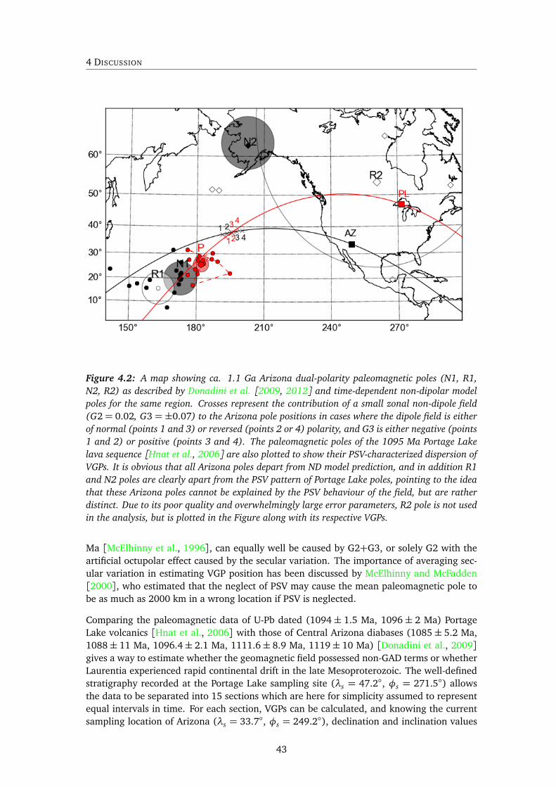
4 DISCUSSION

Figure 4.2: A map showing ca. 1.1 Ga Arizona dual-polarity paleomagnetic poles (N1, R1,N2, R2) as described by Donadini et al. [2009, 2012] and time-dependent non-dipolar modelpoles for the same region. Crosses represent the contribution of a small zonal non-dipole field(G2 = 0.02, G3 = ±0.07) to the Arizona pole positions in cases where the dipole field is eitherof normal (points 1 and 3) or reversed (points 2 or 4) polarity, and G3 is either negative (points1 and 2) or positive (points 3 and 4). The paleomagnetic poles of the 1095 Ma Portage Lakelava sequence [Hnat et al., 2006] are also plotted to show their PSV-characterized dispersion ofVGPs. It is obvious that all Arizona poles depart from ND model prediction, and in addition R1and N2 poles are clearly apart from the PSV pattern of Portage Lake poles, pointing to the ideathat these Arizona poles cannot be explained by the PSV behaviour of the field, but are ratherdistinct. Due to its poor quality and overwhelmingly large error parameters, R2 pole is not usedin the analysis, but is plotted in the Figure along with its respective VGPs.

Ma [McElhinny et al., 1996], can equally well be caused by G2+G3, or solely G2 with theartificial octupolar effect caused by the secular variation. The importance of averaging sec-ular variation in estimating VGP position has been discussed by McElhinny and McFadden[2000], who estimated that the neglect of PSV may cause the mean paleomagnetic pole tobe as much as 2000 km in a wrong location if PSV is neglected.

Comparing the paleomagnetic data of U-Pb dated (1094± 1.5 Ma, 1096± 2 Ma) PortageLake volcanics [Hnat et al., 2006] with those of Central Arizona diabases (1085± 5.2 Ma,1088± 11 Ma, 1096.4± 2.1 Ma, 1111.6± 8.9 Ma, 1119± 10 Ma) [Donadini et al., 2009]gives a way to estimate whether the geomagnetic field possessed non-GAD terms or whetherLaurentia experienced rapid continental drift in the late Mesoproterozoic. The well-definedstratigraphy recorded at the Portage Lake sampling site (λs = 47.2◦, φs = 271.5◦) allowsthe data to be separated into 15 sections which are here for simplicity assumed to representequal intervals in time. For each section, VGPs can be calculated, and knowing the currentsampling location of Arizona (λs = 33.7◦, φs = 249.2◦), declination and inclination values

43

4 DISCUSSION

from Portage Lake can be converted to represent the imagined situation where they areobtained from Arizona.

As seen in Figure 4.1, the Portage Lake mean paleomagnetic direction, as if it were observedin Arizona (D = 281.4◦, I = 51.4◦, α95 = 2.8◦) is statistically distinct from the mean direc-tion of normal-polarity Central Arizona dykes (D = 274.8◦, I = 38.7◦, α95 = 7.6◦). Donadiniet al. [2012] presented U-Pb ages for these Arizona N1 dykes (1085± 5.2 Ma, 1088± 11Ma), but also suggested a new N2 direction (D = 332.6◦, I = 69.4◦, α95 = 3.5◦), which ap-pears clearly anomalous from other Arizona directions, but has an U-Pb age of 1096.4± 2.1Ma, very closely corresponding to that of Portage Lake lavas. The N2 direction, however, isbased on one sampling site only, being merely a VGP. Great uncertainty is also apparent inthe corresponding R2 direction (D = 193.7◦, I = −78.7◦, α95 = 15.7◦), based on five sites.The R1 direction (D = 95.8◦, I = −35.9◦, α95 = 7.8◦), despite being merely from one site,is antiparallel with N1 direction and has not been dated precisely, but is estimated to beroughly 1.1 Ga. Other studies performed on North American rocks of this age are in favourof the theory of symmetric field reversals at 1.1 Ga [Kean et al., 1997, Swanson-Hysell et al.,2009].

Paleomagnetic poles of Arizona dykes reveal that the R1 pole plots slightly farther from thesampling site than the N1 pole does, yet their A95 error limits clearly overlap. The meanPortage Lake pole plots closer to the Arizona sampling site than both Arizona N1 and R1poles do. However, the paleomeridian, which connects Arizona R1 pole to the sampling site,intersects both Arizona N1 and Portage Lake poles, supports the theory of rapid continentaldrift [Swanson-Hysell et al., 2009] and shows no evidence for non-zonal geomagnetic fields.However, the distracting uncertainty apparent in the directional data of Arizona N2 and R2is further strengthened in the pole space and neither of these poles can be considered robustfor studying the North American 1.1 Ga polarity dilemma, although Donadini et al. [2012]put some effort on analyzing their controversial ages. According to PALEOMAGIA database,D = 290◦, I = 55◦ (or D = 110◦, I = −55◦) can be used a working approximation forthe mean direction of 1.07-1.13 Ga Lake Superior rocks, slightly different from the PortageLake mean direction. However, since the paleocolatitudinal difference of Arizona and LakeSuperior is 13◦, the inclination of ±55◦ observed at Portage Lake corresponds to ±64.9◦ asobserved in Arizona.

Using the declination of 292◦ for Arizona and 290◦ for Lake Superior region, the combinedpaleomagnetic pole can be determined as λp = 38◦, φp = 196◦, which is the point wherepaleomeridians of Portage Lake and Arizona intersect in Figure 4.2. The combined effectof a small octupolar field (here G3 = ±0.07) and an even smaller quadrupole field (G2 =0.02) which would be expected according to the findings of this dissertation, cannot shiftthe paleomagnetic pole from its GAD-expected position more than a few degrees, even atmid-latitudes where the ∆(I) value caused by a geocentric axial octupole is at its greatest.However, if G3 is strengthened from 0.07 to 0.20, the error increases and can be as much as6◦ (650 km) in the case where GAD is reversed and G3 is of opposite sign with GAD. Sincethe Lake Superior region is located closer to the paleoequator, the inclination error causedby a possible axial multipole does not propagate to its pole position as much as it propagatesto the pole position of Arizona.

In the last ten years, attempts have been made to create paleogeographic configurations ofcontinents during the Proterozoic [Pesonen et al., 2003] and even Neoarchean [De Kocket al., 2009]. Evidence for the assembly and breakup of continental blocks in the supercon-tinent cycles has been obtained from Precambrian ophiolites [Peltonen et al., 1996], mafic

44

4 DISCUSSION

dyke swarms [Green et al., 1987] large igneous provinces (LIPs) [Ernst and Buchan, 2002]and by comparison of major rifts or orogenic belts [Dalziel, 1997, Li et al., 2003]. Even thepredominantly Archean areas have been bordered by orogenies, volcanic arcs and ancientoceanic terranes. One of the best examples is the early Mesoproterozoic North America,where the unification of Hearne, Superior and Wyoming cratons was characterized by theTrans-Hudson orogen [Whitmeyer and Karlstrom, 2007], which is also visible in Figure 4.4.Very steep inclinations are typical of this area [Harris et al., 2006, Symons, 2007] so even amoderately strong quadrupolar or octupolar contribution in the geomagnetic field would notremarkably shift the area latitudinally in the reconstruction. Had this kind of non-dipolarfield existed, it would cause other parts of the same continent to be at close to the equator,thus requiring one to treat Trans-Hudson separately from the other forming blocks of Lau-rentia which would be in contradiction with the tectonic growth of North America [Evansand Pisarevsky, 2008, Whitmeyer and Karlstrom, 2007].

Knowing the inclination error caused by zonal multipoles, it is possible to investigate howmuch a given zonal contribution to the geomagnetic field affects the positions of continentsin a reconstruction. Figure 4.4 sets an example where the values of 0.02 for G2 and 0.07for G3 have been applied to the reconstruction of early Columbia Nuna at 1.78 Ga, corre-sponding to the recent inclination frequency analysis of 1.5-2.9 Ga rocks (Table 4.1). Bycomparing the result to the corresponding model of Pesonen et al. [2012b], deviations canbe considered minor and in most cases within the A95 uncertainty limits of respective paleo-magnetic poles listed in Table 4.2. More significant differences include the introduction of anew continent (Rio de la Plata), based on the Florida dykes pole [Teixeira et al., 2012], andthe exclusion of Kalahari craton due to the updated age information which shows that thepole of Mashonaland dolerites by McElhinny and Opdyke [1964] is most likely to be 1.87Ga old and hence in line with other Mashonaland poles rather than 1.77 Ga old as previ-ously assumed. The position of Rio de la Plata is shown with a dashed outline and remainsspeculative since the Florida dykes may possess a Phanerozoic remagnetization.

The paleogeography of Ediacaran, the end of the Neoproterozoic, is among the most con-troversial ones, mainly due to the poor paleomagnetic coverage and conflicting poles. Co-existence of very steep and shallow directions with a minimal age difference is demonstratede.g. by the Canadian Sept-Îles layered intrusion and cutting dykes, where the 565± 4 MaA component has yielded an inclination of -29.0◦ and the 535-569 Ma B component has avalue of 82.1◦, respectively [Tanczyk et al., 1987]. Explanations for the situation have beengeomagnetic, e.g. the non-dipolar geomagnetic field, which makes the inclination data mis-leading [Schmidt et al., 1991], or geodynamic, such as the rapid latitudinal motion of plates[Kilner et al., 2005] or true polar wander (TPW) [Evans, 2003]. Theories of low-latitudeglaciations and the Snowball Earth Hypothesis have been presented as well [Kirschvink,1992]. Abrajevitch and Van der Voo [2010] abandoned concepts of apparent or true polarwander but explain two anomalously discordant populations of inclinations within Laurentiaand Baltica by assuming that the geocentric dipole oscillated between axial and equatorialconfigurations between 615 and 555 Ma. In the solar system, large deviations from axialsymmetry are apparent in the current magnetic fields of Uranus and Neptune, but it is un-clear how long they have been operating as such [Holme and Bloxham, 1996], and theyalone cannot justify the theory of equatorial geomagnetic field in the Ediacaran.

Considering the temporally averaged field to be that of a geocentric axial dipole for mostof the Precambrian, with the possible exception of the Ediacaran, justifies the traditionalmethod of APWP comparison in studying whether continents have shared a common his-tory, though paleomagnetic data must be supplemented using information from geological

45

4 DISCUSSION

Table 4.2: Paleomagnetic poles used for the Nuna reconstruction seen in Figure 4.4. I* refers tothe inclination in the case where GAD is supplemented by an axial quadrupole (G2=0.02) andand an axial octupole (G3=0.07) and φ∗p/λ

∗p are the corresponding values for the paleomag-

netic pole. References are as follows: [1] Park et al. [1973], [2] Fedotova et al. [1999], [3] Pis-arevsky and Sokolov [2001], [4] Mertanen et al. [2006], [5] Elming [1985], [6] Veselovskiyet al. [2013], [7] Elming et al. [2009], [8] Bispo-Santos et al. [2008], [9] McElhinny andEvans [1976], [10] Schmidt and Williams [2008], [11] Idnurm [2000], [12] Pradhan et al.[2010], [13] Piper et al. [2011], [14] Zhang et al. [2012], [15] Halls et al. [2000] and [16]Teixeira et al. [2012]. For Baltica, Amazonia and North China, Fisher mean poles of severalrock formations have been used. Abbreviations of continents (Cont.) are similar to those inFigure 4.4.

Cont. Formation D [◦] I/I* [◦] φp/φ∗p[◦] λp/λ

∗p[◦] A95[◦]

L Dubawnt group [1] 347.0 -50.0/-49.7 277.0/276.8 7.0/5.2 8.0B Ropruchey-Ladva

gabbro-dolerites [2] 357.1 23.4/21.3 218.2/218.2 40.7/39.5 5.5

B Shoksha sandstones [3] 354.3 21.6/19.5 221.1/221.0 39.7/38.6 4.0B Lake Ladoga intrusions [4] 347.2 44.2/41.8 229.7/229.1 53.9/51.7 5.9B Vittangi gabbro [5] 339.5 39.1/36.8 227.9/227.4 42.6/42.8 4.9B Pechenga-Verkhnetulomskii

dykes [6] 352.2 11.4/9.3 222.2/220.1 50.4/52.4 10.2

B Hoting gabbro [7] 330.3 40.2/37.9 235.9/235.3 44.3/42.8 10.7B Mean (N=6) 350.0 30.8/28.1 224.0/220.7 41.3/40.5 10.9

Am Colider volcanics [8] 183.0 53.5/50.9 298.8/298.5 -63.3/-67.7 11.4A Hart dolerite [9] 121.0 2.0/-0.2 226.0/227.4 -29.0/-29.4 21.9A Elgee-Pentecost formation

(comb.) [10] 93.9 12.9/10.8 211.8/214.1 -5.4/-5.2 3.2

A Lochness formation [11] 118.9 24.2/22.1 225.6/227.4 -31.2/-30.9 4.2A Mean (N=3) 111.3 13.3/11.2 220.5/221.7 -22.2/-21.9 20.9I Gwalior traps (comb.) [12] 73.9 4.4/2.2 173.2/174.2 15.4/14.9 7.9

NCH Xion dykes and gneisses[13] 9.6 7.4/5.3 277.3/278.1 55.3/53.4 5.2

NCH Xiong’er group [14] 18.4 -3.7/-5.9 263.0/263.7 50.2/49.2 5.4NCH Taihang NNW dyke swarm

[15] 36.0 -5.2/-7.4 247.0/247.7 36.0/35.1 3.0

NCH Mean (N=3) 21.3 -0.5/-2.7 260.9/261.6 47.5/46.4 16.3RLP Florida dykes [16] 9.3 -38.8/-39.5 162.0/161.6 -77.5/-75.8 9.2

46

4 DISCUSSION

2.52.32.11.91.71.51.31.11.0 1.2 1.4 1.6 1.8 2.0 2.2 2.4

Time (Ga)

Equator

Equator

30 S

60 N

30°N

30 N

30 N

30°N

60°N

0

0

0

30 S

30 S

30 S

60 S

Laurentia

Baltica

Amazonia

60 N

60 S

0

60 S

Rodiniasupercontinent

Columbia supercontinent

1.831.10

Break-up of Kenorland

Equator

Equator

Australia

?

2.41.91.51.21.0

Figure 4.3: Latitudinal drifts of Laurentia, Baltica, Amazonia and Australia during the Paleo-and Mesoproterozoic. Paleolatitude is visible on the vertical axis, and geologic age along withdifferent stages of supercontinents are plotted on horizontal axis. Rotations have been calculatedusing the two-step Euler method as explained by Pesonen et al. [2003]. Whenever data arescarce or uncertain, continents are shown with dashed outlines. The validity of GAD hypothesisis assumed. See also Figure 4.4 for the positions of continents 1.78 Ga ago. After Pesonen et al.[2012b], using Karelian craton to present Baltica and Superior craton to present Laurentiabefore 1.8 Ga.

47

4 DISCUSSION

Figure 4.4: A reconstruction of continents at 1.78 Ga. Data available from Laurentia (L),Baltica (B), North China (NC), Amazonia (Am), India (I), Australia (A) and Rio de la Plata(RLP). Archean cratons are marked with grey shading. Major 1.9-1.8 Ga (Nagssugtoqidian asN, Ketilidian as K, Torngat as T, Trans-Hudson as TH, Penokean as P, Woopmay as W, Taltson-Thelon as T-T, Lapland-Kola as L-K, Svecofennian as Sv, Ventuari-Tapajos as V-T and Capricornas C) and 1.8-1.5 Ga orogenic belts (Trans-North China orogen as T-N, Central Indian tectoniczone as C-I, Yavapai as Y, Transscandinavian Igneous Belt as TIB, Rio Negro-Juruena as R-Nand Arunta as Ar) are shown in green. The 1.78-1.70 Ga rapakivi granites are shown as redcircles. Pole positions have been calculated assuming GAD hypothesis to be valid. Positionsof continents remain practically unchanged in the potential case where the inclination dataare slightly distorted from GAD by zonal multipoles (G2=0.02 and G3=0.07) according toTable 4.2.

48

4 DISCUSSION

continuations, such as dyke swarms, rifts, orogenic or accretional belts, kimberlite corridors,rapakivi granite zones etc. [Pesonen et al., 2003]. However, when different-aged paleomag-netic poles are compared, it must be taken into account that the drift rate of continents hasmost probably been much faster in the far past than today. For the Pilbara craton of north-western Australia, Blake et al. [2004] obtained two paleomagnetic results with ages 2721±4and 2718± 3 Ma. The corresponding latitudinal difference is 27◦, yielding to ten times thepresent-day drift rate and five times the fastest drift rate determined for the Phanerozoic.

The supercontinent study of Pesonen et al. [2012b] did not cover the Archean due to thepaucity of high-rated Archean paleomagnetic data. However, in studies of the evolution ofcontinental masses and the geothermal history, the Archean is perhaps the most interestingera in the history of our planet. There is evidence that less than 10% of the continental crustexisted prior to 3.5 Ga, but a rapid rise in crustal formation occurred 2.9-2.6 Ga ago. Roughly70% of the crust was developed before the Birimian orogeny of 2.2 Ga [Stein and Ben-Avraham, 2009]. The reason for the survival of relatively small parts of Archean crust is mostprominently the extensive heat production, which kept the formation and the removal ofcrust close to an equilibrium. The geomagnetic field of that time was, however, according tothe findings of this dissertation, close to the GAD, which makes the models of Pre-Proterozoiccontinents, such as Atlantica, Ur and Nena [Meert, 2002], Kenorland [Pesonen et al., 2003],and Vaalbara [De Kock et al., 2009] paleomagnetically possible.

The question about the best model of the Precambrian geomagnetic field is not easy toanswer due to the small values of required quadrupolar and octupolar components and gen-erally large error limits in datasets. Even though inclination data are widespread, a lesserdegree of certainty is evident when reversal asymmetry and paleosecular variation analysesare used to evaluate the content of the long-term field. Reliable paleomagnetic poles, espe-cially so-called key poles [Buchan et al., 2000], are scarce, and unevenly scattered on theglobe. With the caveats taken into account, the most plausible estimates for average non-dipolar terms of the Precambrian geomagnetic field range from 0% ≤ G2 ≤ 5% of GAD forG2 and 0% ≤ G3 ≤ 10% of GAD for G3. Although the findings of this dissertation supportthe credibility of the GAD hypothesis as a working time-averaged field approximation of thePrecambrian, they cannot disallow the presence of non-dipolar fields in smaller timescales,particularly in the Keweenawan and in the Ediacaran where the controversy of coeval shal-low and steep directions remains unsolved. The general conclusion, however, is a relaxingone for future paleogeographic reconstructions to be made using paleomagnetism as a tool.

49

References

Abrahamsen, N., Pesonen, L., Van der Voo, R., 2001. Palaeomagnetic databases: 4th Nordic Palaeo-magnetic Workshop. Bull. Geol. Soc. Denm. 48, 91–94.

Abrajevitch, A., Van der Voo, R., 2010. Incompatible Ediacaran paleomagnetic directions suggest anequatorial geomagnetic dipole hypothesis. Earth Plan. Sci. Lett. 293, 164–170.

Alfvén, H., 1950. Cosmical Electrodynamics. International Series of Monographs on Physics, Claren-don Press. 237pp.

Arkani-Hamed, J., Strangway, D., 1986. Band-limited global scalar magnetic anomaly map of theEarth derived from Magsat data. J. Geophys. Res. 91, 8193–8203.

Bazhenov, M., Shatsillo, A., 2010. Late Permian palaeomagnetism of Northern Eurasia: data evalua-tion and a single-plate test of the geocentric axial dipole model. Geophys. J. Int. 180, 136–146.

Biggin, A., Strik, G., Langereis, C., 2008. Evidence for a very long term trend in secular variation.Nature Geoscience 1, 395–398.

Bingen, B., Mansfeld, J., Sigmond, E., Stein, H., 2002. Baltica-Laurentia link during the Mesoprotero-zoic: 1.27 Ga development of continental basins in the Sveconorwegian Orogen, southern Norway.Can. J. Earth Sci. 39, 1425–1440.

Bingham, D., Evans, M., 1976. Paleomagnetism of the Great Slave Supergroup, Northwest Territo-ries, Canada: the Stark Formation. Can. J. Earth Sci. 13, 563–578.

Bispo-Santos, F., D’Agrella-Filho, M., Pacca, I., Janikian, L., Trindade, R., Elming, S.Å., Silva, J.,Barros, M., Pinhno, F., 2008. Columbia revisited: Paleomagnetic results from the 1790 Ma Colidervolcanics (SW Amazonian Craton, Brazil). Prec. Res. 164, 40–49.

Blake, T., Buick, R., Brown, S., Barley, M., 2004. Geochronology of Late Archaean flood basaltprovince in the Pilbara Craton, Australia: Constraints on basin evolution, volcanic and sedimentaryaccumulation, and continental drift rates. Prec. Res. 133, 143–173.

Bloxham, J., 2000. Sensitivity of the geomagnetic axial dipole to thermal core-mantle interactions.Nature 405, 63–65.

Briden, J., Duff, B., 1981. Pre-Carboniferous paleomagnetism of Europe north of the Alpine oro-genic belt. In: M.W. McElhinny, D.A. Valencio (eds.) "Paleoreconstruction of the Continents", AGUGeodynamics Series 2, pp. 137–150.

Brown, L., McEnroe, S., 2012. Paleomagnetism and magnetic mineralogy of Grenville metamorphicand igneous rocks, Adirondack Highlands, USA. Prec. Res. 212-213, 57–74.

Brunhes, B., 1906. Recherches sur le direction d’aimantation des roches volcaniques. J. Phys. 5,705–724.

Buchan, K., 2013. Key paleomagnetic poles and their use in Proterozoic continent and supercontinentreconstructions: A review. Prec. Res. 238, 93–110.

Buchan, K., Halls, H., 1990. Paleomagnetism of Proterozoic mafic dyke swarms of the Canadianshield. In: A.J. Parker, P.C. Rickwood, D.H. Tucker (eds.), "Mafic Dikes and Emplacement Mecha-nisms", Balkema, Rotterdam, pp. 209–230.

50

Buchan, K., LeCheminant, A., Van Breemen, O., 2012. Malley Diabase Dykes of the Slave craton,Canadian shield: U-Pb age, paleomagnetism, and implications for continental reconstructions inthe early Paleoproterozoic. Can. J. Earth Sci. 49, 435–454.

Buchan, K., Mertanen, S., Park, R., Pesonen, L., Elming, S.Å., Abrahamsen, N., Bylund, G., 2000.Comparing the drift of Laurentia and Baltica in the Proterozoic: the importance of key paleomag-netic poles. Tectonophys. 319, 167–198.

Butler, R., 1992. Paleomagnetism: Magnetic Domains to Geologic Terranes. Blackwell ScientificPublications. 336pp.

Carporzen, L., Weiss, B., Gilder, S., Pommier, A., Hart, R., 2012. Lightning remagnetization of theVredefort impact crater: No evidence for impact-generated magnetic fields. J. Geophys. Res. 117,E01007.

Channell, J., 2006. Late Brunhes polarity excursions (Mono Lake, Laschamp, Iceland Basin andPringle Falls) recorded at ODP Site 919 (Irminger Basin). Earth. Plan. Sci. Lett. 244, 378–393.

Chapman, S., Bartels, J., 1940. Geomagnetism, Vols 1 and 2, 2nd edition. Oxford University Press,Oxford. 542pp.

Clement, B., 2004. Dependence of the duration of geomagnetic polarity reversals on site latitude.Nature 428, 637–640.

Coe, R., 1979. The effect of shape anisotropy on TRM direction. Geophys. J. Roy. Astr. Soc. 56,369–383.

Coe, R., Glatzmaier, G., 2006. Symmetry and stability of the geomagnetic field. Geophys. Res. Lett.33, L21311.

Cogné, J., Halim, N., Chen, Y., Courtillot, V., 1999. Resolving the problem of shallow magnetizationsof Tertiary age in Asia: insights from paleomagnetic data from the Qiangtang, Kunlun, and Qaidamblocks (Tibet, China), and a new hypothesis. J. Geophys. Res. 104, 17715–17734.

Condie, K., 1997. Plate Tectonics and Crustal Evolution. Butterworth-Heinemann, Oxford. 288pp.

Constable, C., 2000. On rates of occurrence of geomagnetic reversals. Phys. Earth. Plan. Int. 118,181–193.

Constable, C., Parker, R., 1988. Statistics of the geomagnetic secular variation for the past 5 m.y. J.Geophys. Res. 83, 11569–11581.

Costanzo-Alvarez, V., Dunlop, D., 1998. A regional paleomagnetic study of lithotectonic domains inthe Central Gneiss Belt, Grenville Province, Ontario. Earth Plan. Sci. Lett. 160, 89–103.

Costanzo-Alvarez, V., Dunlop, D., Pesonen, L., 1993. Paleomagnetism of alkaline complexes andremagnetization in the Kapuskasing Structural Zone, Ontario, Canada. J. Geophys. Res. 98, 4063–4079.

Courtillot, V., Le Mouël, J.L., 2007. The study of Earth’s magnetism (1269-1950): A foundation byPeregrinus and subsequent development of geomagnetism and paleomagnetism. Rev. Geophys. 45,RG3008.

Cowling, T., 1955. The magnetic field of sunspots. Month. Not. Roy. Astr. Soc., Geophysical Supple-ment 94, 39–48.

Cox, A., 1975. The frequency of geomagnetic reversals and the symmetry of the non-dipole field.Rev. Geophys. 13, 35–51.

Cox, A., Doell, R., 1960. Review of paleomagnetism. Geol. Soc. Am. Bull. 71, 645–768.

Creer, K., Georgi, D., Lowrie, W., 1973. On the representation of the Quaternary and late Tertiarygeomagnetic field in terms of dipoles and quadrupoles. Geophys. J. Roy. Astr. Soc. 33, 323–345.

Creer, K., Irving, E., Nairn, A., 1959. The palaeomagnetism of the Great Whin Sill. Geophys. J. Roy.Astr. Soc. 2, 306–323.

Creer, K., Irving, E., Runcorn, S., 1954. The direction of geomagnetic field in remote epochs in GreatBritain. J. Geomagn. Geoelectr. 6, 163–168.

51

D’Agrella-Filho, M., Pacca, I., Trindade, R., Teixeira, W., Raposo, M., Onstott, T., 2004. Paleomag-netism and 40Ar/39Ar ages of mafic dikes from Salvador (Brazil): new constraints on the SaoFrancisco craton APW path between 1080 and 1010 Ma. Prec. Res. 132, 55–77.

Dalziel, I., 1997. Neoproterozoic-Paleozoic geography and tectonics: review, hypothesis, environ-mental speculation. Geol. Soc. Am. Bull. 109, 16–42.

David, P., 1904. Sur la stabilité de la direction d’aimantation dans quelques roches volcaniques. C. R.Acad. Sci. Paris 138, 41–42.

De Kock, M., Evans, D., Beukes, N., 2009. Validating the existence of Vaalbara in the Neoarchean.Prec. Res. 169, 80–99.

Dominguez, A., Van der Voo, R., 2014. Secular variation of the middle and late Miocene geomag-netic field recorded by the Columbia River Basalt Group in Oregon, Idaho and Washington, USA.Geophys. J. Int. 197, 1299–1320.

Donadini, F., 2007. Features of the geomagnetic field during the Holocene and Proterozoic. Ph.D.thesis. Division of Geophysics, University of Helsinki, 188pp.

Donadini, F., Pesonen, L., Korhonen, K., Deutsch, A., Harlan, S., 2009. Paleomagnetism and Paleoin-tensity of the 1.1 Ga Old Diabase Sheets from Central Arizona. Geophysica 47, 3–30.

Donadini, F., Pesonen, L., Korhonen, K., Deutsch, A., Harlan, S., Heaman, L., 2012. Symmetricand asymmetric reversals in the 1.1 Ga Central Arizona diabases: The debate continues. In: S.Mertanen, L.J. Pesonen, P. Sangchan (eds.), "Supercontinent Symposium 2012. Programme andAbstracts", pp. 35–36.

Donadini, F., Riisager, P., Korhonen, K., Kahma, K., Pesonen, L., Snowball, I., 2007. Holocene geo-magnetic paleointensities: A blind test of absolute paleointensity techniques and materials. Phys.Earth. Plan. Int. 161, 19–35.

Doubrovine, P., Steinberger, B., Torsvik, T., 2012. Absolute plate motions in a reference frame definedby moving hot spots in the Pacific, Atlantic, and Indian oceans. J. Geophys. Res. 117, B09101.

DuBois, P., 1962. Paleomagnetism and correlation of Keweenawan rocks. Bull. Geol. Surv. Can. 71,1–75.

Dunlop, D., Yu, Y., 2004. Intensity and Polarity of the Geomagnetic Field During Precambrian Time.In: J.E.T. Channell, D.V. Kent, W. Lowrie, J.G. Meert (eds.) "Timescales of the Paleomagnetic Field",AGU Geophysical Monograph 145, pp. 85–99.

Elming, S.Å., 1985. A palaeomagnetic study of Svecokarelian basic rocks from northern Sweden.Geol. Fören. Förhandlingar 107, 17–35.

Elming, S.Å., Moakhar, M., Layer, P., Donadini, F., 2009. Uplift deduced from remanent magnetizationof a proterozoic basic dyke and the baked country rock in the Hoting area, Central Sweden: apalaeomagnetic and 40Ar/39Ar study. Geophys. J. Int. 179, 59–78.

Elming, S.Å., Pisarevsky, S., Layer, P., Bylund, G., 2014. A palaeomagnetic and 40Ar/39Ar study ofmafic dykes in southern Sweden: A new early Neoproterozoic key-pole for the Baltic shield andimplications for Sveconorwegian and Grenville loops. Prec. Res., 244, 192–206.

Elsasser, W., 1939. On the origin of the Earth’s magnetic field. Phys. Rev. 55, 489–498.

Elston, D., Enkin, R., Baker, J., Kisilevsky, D., 2002. Tightening the Belt: Paleomagnetic-stratigraphicconstraints on deposition, correlation, and deformation of the Middle Proterozoic (ca. 1.4 Ga)Belt-Purcell Supergroup, United States and Canada. Geol. Soc. Am. Bull. 114, 619–638.

Ernst, R., Buchan, K., 1993. Paleomagnetism of the Abitibi dyke swarm, southern Superior Province,and implications for the Logan Loop. Can. J. Earth Sci. 30, 1886–1897.

Ernst, R., Buchan, K., 2002. Maximum size and distribution in time and space of mantle plumes:evidence from large igneous provinces. J. Geodyn. 34, 309–342.

Evans, D., 2003. True polar wander and supercontinents. Tectonophys. 362, 303–320.

Evans, D., 2006. Proterozoic low orbital obliquity and axial-dipolar geomagnetic field from evaporite

52

palaeolatitudes. Nature 444, 51–55.

Evans, D., Li, Z., Kirschvink, J., Wingate, M., 2000. A high quality mid-Neoproterozoic paleomagneticpole from South China, with implications for ice ages and the breakup configuration of Rodinia.Prec. Res. 100, 313–334.

Evans, D., Mitchell, R., 2011. Assembly and breakup of the core of Paleoproterozoic-Mesoproterozoicsupercontinent Nuna. Geol. Soc. Am. Bull. 39, 443–446.

Evans, D., Pisarevsky, S., 2008. Plate tectonics on the early earth? - Weighing the paleomagneticevidence. In: K. Condie, V. Pease (eds.), "When did Plate Tectonics Begin", Geol. Soc. Am. Sp.Paper, pp. 137–150.

Evans, M., 1976. Test of the dipolar nature of the geomagnetic field throughout Phanerozoic time.Nature 262, 676–677.

Evans, M., 2005. Testing the geomagnetic dipole hypothesis: paleolatitudes sampled by large conti-nents. Geophys. J. Int. 161, 266–267.

Evans, M., 2012. Magnetostratigraphy of the Lodève Basin, France: Implications for the Permo-Carboniferous reversed superchron and the geocentric axial dipole. Studia Geophysica et Geodaet-ica 56, 725–734.

Everitt, C., Clegg, J., 1962. A field test of paleomagnetic stability. Geophys. J. Roy. Astr. Soc. 6,312–319.

Fedotova, M., Khramov, A., Pisakin, B., Priyatkin, A., 1999. Early Proterozoic palaeomagnetism: newresults from the intrusive and related rocks of the Karelian, Belomorian and Kola provinces, easternFennoscandian shield. Geophys. J. Int. 137, 691–712.

Fisher, R., 1953. Dispersion on a sphere. Proc. Roy. Soc. London A217, 295–305.

Gallet, Y., Pavlov, V., Semikhatov, M., Petrov, P., 2005. Late Mesoproterozoic magnetostratigraphicresults from Siberia: Paleogeographic implications and magnetic field behavior. J. Geophys. Res.105, 16481–16499.

Gibbons, S., 1998. The Parker-Levy reversal mechanism. Phys. Earth. Plan. Int. 106, 129–137.

Giddings, J., Idnurm, M., 1993. Significance of overprint magnetizations in the PaleoproterozoicKombolgie Formation, western McArthur Basin, N.T. Exploration Geophysics (Melbourne) 24,231–237.

Glatzmaier, G., Roberts, P., 1996. An anelastic evolutionary geodynamo simulation driven by compo-sitional and thermal convection. Physica D97, 81–94.

Gose, W., Hanson, R., Dalziel, I., Pancake, J., Seidel, E., 2006. Paleomagnetism of the 1.1 GaUmkondo large igneous province in southern Africa. J. Geophys. Res. 111, 1–18.

Green, J., Bornhorst, T., Chandler, V., Mudrey Jr., M., Myers, P., Pesonen, L., Wilband, J., 1987.Keweenawan Dykes of the Lake Superior Region: Evidence for Evolution of the Middle Proterozoic.In: H.C. Halls, W.F. Fahrig (eds.), "Mafic Dyke Swarms", GAC Sp. Paper, pp. 289–302.

Gubbins, D., 1999. The distinction between geomagnetic excursions and reversals. Geophys. J. Int.137, F1–F3.

Gubbins, D., Coe, R., 1993. Longitudinally confined geomagnetic reversal paths from non-dipolartransition fields. Nature 362, 51–53.

Haines, G., 1985. Spherical Cap Harmonic Analysis. J. Geophys. Res. 90, 2583–2591.

Halley, E., 1715. Some remarks on the variations of the magnetical compass published in the Memoirsof the Royal Academy of Sciences, with regard to the general chart of those variations made byE. Halley; as also concerning the true longitude of the Magellan Straights. Phil. Trans. Roy. Soc.,Series A 29(341), 165–168.

Halls, H., Kumar, A., Srinivasan, R., Hamilton, M., 2000. A precisely dated Proterozoic palaeomag-netic pole from the North China craton, and its relevance to palaeocontinental reconstruction.Geophys. J. Int. 143, 185–203.

53

Halls, H., Kumar, A., Srinivasan, R., Hamilton, M., 2007. Paleomagnetism and U-Pb geochronologyof easterly trending dykes in the Dharwar craton,India: feldspar clouding,radiating dyke swarmsand the position of India at 2.37 Ga. Prec. Res. 155, 47–68.

Hansteen, H., 1819. Untersuchungen über den Geomagnetismus der Erde. Christiania. 358pp.

Harris, M., Symons, D., Blackburn, W., Turek, A., Peck, D., 2006. Paleomagnetism of the WinteringLake pluton and the Early Proterozoic tectonic motion of the Superior Boundary Zone, Manitoba.Can. J. Earth Sci. 43, 1071–1083.

Harrison, C., 1995. Secular Variation of the Earth’s Magnetic Field. J. Geomagn. Geoelectr. 47,131–147.

Hatakeyama, T., Kono, M., 2009. Shift of the mean magnetic field values:: Effect of scatter due tosecular variation and errors. Earth Planets Space 53, 31–44.

Heimpel, M., Evans, M., 2013. Testing the geomagnetic dipole and reversing dynamo models overEarth’s cooling history. Phys. Earth Plan. Int. 224, 124–131.

Hnat, J., Van der Pluijm, B., Van der Voo, R., 2006. Primary curvature in the Mid-Continent Rift:Paleomagnetism of the Portage Lake Volcanics (northern Michigan, USA). Tectonophys. 425, 71–82.

Hoffman, K., 1977. Polarity transition records and the geomagnetic dynamo. Science 196, 1329–1332.

Hoffman, K., 1981. Paleomagnetic excursions, aborted reversals and transitional fields. Nature 294,67–69.

Holme, R., Bloxham, J., 1996. The magnetic fields of Uranus and Neptune; methods and models. J.Geophys. Res. 101, 2177–2200.

Holme, R., De Viron, O., 2005. Geomagnetic jerks and a high-resolution length-of-day profile for corestudies. Geophys. J. Int. 160, 435–439.

Hospers, J., 1954. Rock magnetism and polar wandering. Nature 173, 1183–1184.

Hou, G., Kusky, T., Wang, C., Wang, Y., 2010. Mechanics of the giant radiating Mackenzie dykeswarm: A paleostress field modeling. J. Geophys. Res. 115, B02402.

IAGA, 2010. International Geomagnetic Reference Field: the eleventh generation. International As-sociation of Geomagnetism and Aeronomy Working Group V-MOD (Finlay, C.C., Maus, S., Beg-gan, C.D., Bondar, T.N., Champodut, A., Chernova, T.A., Chulliat, A., Golovkov, V.P., Hamilton, B.,Hamoudi, M. Holme, R., Hulot, G., Kuang, W., Langlais, B., Lesur, V., Lowes, F.J., Lühr, H., Macmil-lan, S., Mandea, M., McLean, S., Manoj, C., Menvielle, M., Michaelis, I., Olsen, N., Rauberg,J., Rother, M., Sabaka, T.J., Tangborn, A., Tøffner-Clausen, L., Thébault, E., Thomson, A.W.P.,Wardinski, I., Wei, Z. and Zvereva, T.I.). Geophys. J. Int. 183, 1216–1230.

Idnurm, N., 2000. Towards a high resolution Late Palaeoproterozoic - earliest Mesoproterozoic ap-parent polar wander path for northern Australia. Aust. J. Earth Sci. 47, 405–429.

Irving, E., 1964. Palaeomagnetism and its application to geological and geophysical problems. JohnWiley & Sons. 399pp.

Irving, E., 2005. Palaeomagnetic and palaeoclimatological aspects of polar wandering. Geofis. PuraAppl. 33, 23–41.

Irving, E., Tanczyk, E., Hastie, J., 1976. Catalogue of paleomagnetic directions and poles. Geomag-netic Service of Canada, Ottawa Geomagnetic Series 6. 70pp.

Irving, E., Ward, M., 1964. A statistical model of the geomagnetic field. Pure Appl. Geophys. 57,47–52.

Jarboe, N., Koppers, A., Tauxe, L., Minnett, R., Constable, C., 2012. GP31A-1063: The Online MagICDatabase: Data Archiving, Compilation, and Visualization for the Geomagnetic, Paleomagnetic andRock Magnetic Communities. AGU Fall Meeting, abstract.

Johansson, A., 2009. Baltica, Amazonia and the SAMBA connection - 1000 million years of neigh-

54

bourhood during the Proterozoic? Prec. Res. 175, 221–234.

Johnson, C., Constable, C., 2008. Recent investigations of the 0-5 Ma geomagnetic field recorded bylava flows. Geochemistry Geophysics Geosystems 9, Q04032.

Jones, D., Bates, M., Li, Z., Corner, B., Hodgkinson, G., 2003. Paleomagnetic results from the ca. 1130Ma Borgmassivet intrusions in the Ahlmannryggen region of Dronning Maud Land, Antarctica, andtectonic implications. Tectonophys. 375, 247–260.

Jones, G., Maki, D., 2005. Lightning induced magnetic anomalies on archaeological sites. Archaeo-logical Prospection 12, 191–197.

Kean, W., Williams, I., Chan, L., Feeney, J., 1997. Magnetism of the Keweenawan age Chengwatanalava flows, northwest Wisconsin. Geophys. Res. Lett. 24, 1523–1526.

Kent, D., Irving, E., 2010. Influence of inclination error in sedimentary rocks on the Triassic andJurassic apparent pole wander path for North America and implications for Cordilleran tectonics.J. Geophys. Res. 115, B10103.

Kent, D., Smethurst, M., 1998. Shallow bias of paleomagnetic inclinations in the Paleozoic andPrecambrian. Earth Plan. Sci. Lett. 160, 391–402.

Khramov, A., 1971. Paleomagnetic directions and pole positions: Data for the USSR. Soviet Geophys-ical Committee, World Data Center B, No. 1.

Khramov, A., 1979. Paleomagnetic directions and pole positions: Data for the USSR. Soviet Geophys-ical Committee, World Data Center B, No. 4.

Kilner, B., MacNiocall, C., Brasier, M., 2005. Low-latitude glaciation in the Neoproterozoic of Oman.Geology 33, 413–416.

King, R., 1955. The remanent magnetism of artificially deposited sediments. Month. Not. Roy. Astr.Soc., Geophysical Supplement 7, 115–134.

Kirschvink, J., 1992. Late Proterozoic low-latitude global glaciation: the snowball Earth. In: J.W.Schopf, C. Klein (eds.), "The Proterozoic Biosphere", Cambridge University Press, pp. 51–52.

Komissarova, R.A., I.A.K.A., 1997. Geomagnetic reversals recorded in the Late Riphean Katav forma-tion, South Urals. Izvestiya, Phys. Solid Earth 33, 139–146.

Korhonen, J., 1999. Preliminary magnetic and gravity anomaly maps of the Fennoscandian shield 1:10 000 000. Geol. Surv. Fin. Sp. Paper 27, 173–179.

Korhonen, K., Donadini, F., Riisager, P., Pesonen, L., 2008a. GEOMAGIA50: An archeointensitydatabase with PHP and MySQL. Geochem. Geophys. Geosyst. 9, Q04029.

Korhonen, K., Pesonen, L., Evans, D., Smirnov, A., 2008b. A series of five criteria to test the GeocentricAxial Dipole (GAD) hypothesis in paleomagnetism, in: Geophysical Research Abstracts, EGU, pp.SRef–ID 1607–7962/gra/EGU2008–A–04274.

Labrosse, S., Poirier, J.P., Le Mouël, J.L., 2001. The age of the inner core. Earth Plan. Sci. Lett. 190,111–123.

Laj, C., Guillou, H., Szeremeta, N., Coe, R., 1999. Geomagnetic paleosecular variation at Hawaiiaround 3 Ma from a sequence of 107 lava flows at Kaena Point (Oahu). Earth Plan. Sci. Lett. 170,365–376.

Langlais, B., Purucker, M., Mandea, M., 2004. Crustal magnetic field of Mars. J. Geophys. Res. 109,E02008.

Levashova, N., Gibsher, A., Meert, J., 2011a. Precambrian Microcontinents of the Ural-MongolianBelt: New Paleomagnetic and Geochronological Data. Geotectonics 45, 51–70.

Lewchuk, M., Symons, D., 1990. Paleomagnetism of the Late Precambrian Coldwell Complex, On-tario, Canada. Tectonophys. 184, 73–86.

Li, Z., 2000. Paleomagnetic evidence for unification of the North and West Australian cratons by ca.1.7 Ga: new results from the Kimberley basin of northwestern Australia. Geophys. J. Int. 142,173–180.

55

Li, Z., Cho, M., Li, X.H., 2003. Precambrian tectonics of East Asia and relevance to supercontinentevolution. Prec. Res. 122, 1–6.

Loper, D., McCartney, K., 1986. Mantle plumes and the periodicity of magnetic field reversals. Geo-phys. Res. Lett. 13, 1525–1528.

Lowes, F., 1966. Mean-square values on sphere of spherical harmonic fields. J. Geophys. Res. 71,2179.

Lowes, F., 1974. Spatial power spectrum of the main geomagnetic field extrapolation to the core.Geophys. J. Roy. Astr. Soc. 36, 717–730.

Maloof, A., Halverson, G., Kirschvink, J., Schrag, D., Weiss, B., Hoffman, P., 2006. Combinedpaleomagnetic, isotopic and stratigraphic evidence for true polar wander in the NeoproterozoicAkademikerbreen Group. Geol. Soc. Am. Bull. 118, 1099–1124.

Maus, S., 2008. The geomagnetic power spectrum. Geophys. J. Int. 174, 135–142.

McElhinny, M., 2004. Geocentric axial dipole hypothesis: a least squares perspective. In: J.E.T.Channell, D.V. Kent, W. Lowrie, J.G. Meert (eds.) "Timescales of the Paleomagnetic Field", AGUGeophysical Monograph 145, pp. 1–12.

McElhinny, M., Cowley, J., 1977. Paleomagnetic directions and pole positions. XIV. Geophys. J. Roy.Astr. Soc. 49, 313–356.

McElhinny, M., Evans, M., 1976. Palaeomagnetic results from the Hart dolerite of the KimberleyBlock, Australia. Prec. Res. 3, 231–241.

McElhinny, M., Lock, J., 1996. IAGA paleomagnetic databases with Access. Surv. Geophys. 17, 575–591.

McElhinny, M., McFadden, P., 1997. Paleosecular variation over the past 5 Myr based on a newgeneralized database. Geophys. J. Int. 131, 240–252.

McElhinny, M., McFadden, P., 2000. Paleomagnetism: Continents and Oceans. Academic Press, SanDiego. 386pp.

McElhinny, M., McFadden, P., Merrill, R., 1996. The time-averaged paleomagnetic field 0-5 Ma. J.Geophys. Res. 101, 25007–25027.

McElhinny, M., Opdyke, N., 1964. The paleomagnetism of the Precambrian dolerites of eastern SouthRhodesia. An example of geologic correlation by rock magnetism. Geophys. J. Int. 69, 2465–2475.

McFadden, P., 2004. Is 600 Myr long enough for the random palaeogeographic test of the geomagneticaxial dipole assumption? Geophys. J. Int. 158, 443–445.

McFadden, P., McElhinny, M., 1984. A physical model for palaeosecular variation. Geophys. J. Roy.Astr. Soc. 78, 809–823.

McFadden, P., Merrill, R., McElhinny, M., 1988. Dipole/quadrupole family modeling of paleosecularvariation. J. Geophys. Res. 93, 11583–11588.

Meert, J., 2002. Paleomagnetic Evidence for a Paleo-Mesoproterozoic Supercontinent Columbia.Gond. Res. 5, 207–215.

Meert, J., Nedelec, A., Hall, C., 2003a. The stratoid granites of central Madagascar: paleomagnetismand further age constraints on Neoproterozoic deformation. Prec. Res. 120, 101–129.

Meert, J., Tamrat, E., Spearman, J., 2003b. Non-dipole fields and inclination bias: insights from arandom walk analysis. Earth Plan. Sci. Lett. 214, 395–408.

Meert, J., Torsvik, T., 2003. The making and unmaking of a supercontinent: Rodinia revisited.Tectonophys. 375, 261–288.

Merrill, R., McElhinny, M., McFadden, P., 1998. The Magnetic Field of the Earth. Paleomagnetism,the Core and the Deep Mantle. Academic Press, San Diego. 531pp.

Mertanen, S., Hölttä, P., Pesonen, L., Paavola, J., 2006. Paleomagnetism of Paleoproterozoic doleritedykes in central Finland. ). In: E. Hanski, S. Mertanen, T. Rämo, J. Vuollo (eds.) "Dyke Swarms -

56

Time Markers of Crustal Evolution", Taylor-Francis, London, pp. 243–256.

Middleton, R., Borradaile, G., Baker, D., Lucas, K., 2004. Proterozoic diabase sills of northern Ontario:magnetic properties and history. J. Geophys. Res. 109.

Mutanen, T., Huhma, H., 2003. The 3.5 Ga Siurua trondhjemite gneiss in the Archean PudasjärviGranulite Belt, northern Finland. Bull. Geol. Soc. Fin. 75, 51–68.

Nevanlinna, H., Pesonen, L., 1983. Late Precambrian Keweenawan asymmetric polarities as analyzedby axial offset dipole geomagnetic models. J. Geophys. Res. 88, 645–658.

Nevanlinna, H., Rynö, J., Haines, G., Borg, K., 1988. Spherical cap harmonic analysis applied to theScandinavian geomagnetic field 1985.0. Deutsche Hydrografische Zeitschrift 41, 177–186.

Ogg, J., Agterberg, F., Gradstein, F., 2004. The Cretaceous period. In: F.M. Gradstein, J.G. Ogg, A.G.Smith (eds.) "A Geologic Time Scale 2004", Cambridge University Press, pp. 344–383.

Ogg, J., Smith, A., 2004. The geomagnetic polarity time scale. In: F.M. Gradstein, J.G. Ogg, A.G.Smith (eds.) "A Geologic Time Scale 2004", Cambridge University Press, pp. 63–86.

Olson, P., 2007. Gravitational dynamos and the low-frequency secular variation. Proc. Natl. Acad. SciUSA 104, 20159–20166.

Opdyke, N., 1969. A test of the dipole hypothesis. Earth Plan. Sci. Lett. 6, 139–151.

Opdyke, N., Channell, J., 1996. Magnetic Stratigraphy. Academic Press, San Diego. 346pp.

Palais, B., Palais, R., Rodi, S., 2009. A disorienting look at Euler’s theorem on the axis of rotation.Am. Math. Month. 116, 892–909.

Palmer, H., 1970. Paleomagnetism and correlation of some Middle Keweenawan rocks, Lake Superior.Can. J. Earth Sci. 7, 1410–1436.

Panzik, J., Evans, D., 2012. GP31B-1070: Proterozoic geomagnetic field geometry from mafic dykeswarms. AGU Fall Meeting, abstract.

Parés, J., Van der Voo, R., 2013. Non-antipodal directions in magnetostratigraphy: an overprint bias?Geophys. J. Int. 192, 75–81.

Park, J., Irving, E., Donaldson, J., 1973. Paleomagnetism of the Precambrian Dubawnt Group. Geol.Soc. Am. Bull. 84, 859âAS870.

Pavlov, V., Gallet, Y., 2009. The Katav Limestones: a Unique Example of Remagnetization or an IdealRecorder of the Neoproterozoic Geomagnetic Field. Izvestiya, Phys. Solid Earth 45, 31–40.

Peltonen, P., Kontinen, A., Huhma, H., 1996. Petrology and geochemistry of metabasalts from the1.95 Ga Jormua ophiolite, northeastern Finland. J. Petr. 37, 1359–1383.

Perrin, M., Shcherbakov, V., 1995. Paleointensity of the Earth’s magnetic field for the past 400 Ma:Evidence for a dipole structure during the Mesozoic low. J. Geomagn. Geoelectr. 49, 601–614.

Pesonen, L., 1979. Paleomagnetism of Late Precambrian Keweenawan igneous and baked contactrocks from Thunder Bay district, northern Lake Superior. Bull. Geol. Soc. Fin. 51, 27–44.

Pesonen, L., 1987. Scandinavian paleomagnetists meet. EOS Trans. Am. Geophys. Union 68, 1157.

Pesonen, L., Elming, S.Å., Mertanen, S., Pisarevsky, S., D’Agrella-Filho, M., Meert, J., Schmidt, P.,Abrahamsen, N., Bylund, G., 2003. Paleomagnetic configuration of continents during the Protero-zoic. Tectonophys. 375, 289–324.

Pesonen, L., Evans, D., Veikkolainen, T., Sangchan, P., 2012. A novel Precambrian paleomagneticdatabase: The basis for analysing supercontinents, GAD and PSV. In: S. Mertanen, L.J. Pesonen, P.Sangchan (eds.), "Supercontinent Symposium 2012. Programme and Abstracts", pp. 104–105.

Pesonen, L., Mertanen, S., Veikkolainen, T., 2012b. Paleo-Mesoproterozoic Supercontinents - A Pale-omagnetic View. Geophysica 48, 5–47.

Pesonen, L., Neuvonen, K., 1981. Paleomagnetism of the Baltic Shield - implications for Precambriantectonics. In: A. Kröner (ed.), "Precambrian Plate Tectonics", Elsevier, Amsterdam, pp. 623–648.

57

Pesonen, L., Nevanlinna, H., 1981. Late Precambrian Keweenawan asymmetric reversals. Nature294, 436–439.

Pesonen, L., Nevanlinna, H., Leino, M., Rynö, J., 1994. The Earth’s Magnetic Field Maps of 1990.0.Geophysica 30, 57–77.

Piper, J., 1982. The Precambrian paleomagnetic record: the case for the Proterozoic supercontinent.Earth Plan. Sci. Lett. 59, 61–89.

Piper, J., Grant, S., 1989. A paleomagnetic test of the axial dipole assumption and implications forcontinental distributions through geological time. Phys. Earth Plan. Int. 55, 37–53.

Piper, J., Jiasheng, Z., Huang, B., Roberts, A., 2011. Palaeomagnetism of Precambrian dyke swarmsin the North China Shield: The 1.8 LIP event and crustal consolidation in late Palaeoproterozoictimes. J. Asian Earth Sci. 41, 504–524.

Pisarevsky, S., 2005. New edition of the Global Paleomagnetic Database. EOS Trans. Am. Geophys.Union 86, 170.

Pisarevsky, S., Bylund, G., 2006. Palaeomagnetism of 935 Ma mafic dykes in southern Sweden andimplications for the Sveconorwegian Loop. Geophys. J. Int. 166, 1095–1104.

Pisarevsky, S., Sokolov, S., 2001. The magnetostratigraphy and a 1780 Ma palaeomagnetic pole fromthe red sandstones of the Vazhinka River section, Karelia, Russia. Geophys. J. Int. 146, 531–538.

Poorter, R., 1981. Precambrian paleomagnetism of Europe and the position of the Balto-Russian platerelative to Laurentia. In: A. Kröner (ed.), "Precambrian Plate Tectonics", Elsevier, Amsterdam, pp.599–622.

Pradhan, V., Meert, J., Pandit, M., Kamenov, G., Erfan Ali Mondal, M., 2012. Paleomagnetic andgeochronological studies of the mafic dyke swarms of Bundelkhand craton, central India: implica-tions for the tectonic evolution and paleogeographic reconstructions. Prec. Res. 198-199, 51–76.

Pradhan, V., Meert, J., Pandit, M., Kamenov, G., Gregory, L., Malone, S., 2010. IndiaâAZs changingplace in global Proterozoic reconstructions: A review of geochronologic constraints and paleomag-netic poles from the Dharwar, Bundelkhand and Marwar cratons. J. Geodyn. 50, 224–242.

Rämö, O., Haapala, I., 1995. One hundred years of Rapakivi Granite. Mineralogy and Petrology 52,129–185.

Roy, L., Robertson, W., 1978. Paleomagnetism of the Jacobsville Formation and the apparent polarpath for the interval -1100 to -670 m.y. for North America. J. Geophys. Res. 83, 1289–1304.

Runcorn, S., 1954. The Earth’s Core. Trans. Am. Geophys. Union 53, 49–63.

Runcorn, S., 1956. Paleomagnetic comparisons between Europe and North America. Proc. Geol.Assoc. Canada 8, 77–85.

Runcorn, S., 1959. On the hypothesis that the mean geomagnetic field for parts of geological timehas been that of a geocentric axial multipole. J. Atmos. Terr. Phys. 14, 167–174.

Salminen, J., Pesonen, L., Lahti, K., Kannus, K., 2013. Lightning-induced remanent magnetization inthe Vredefort impact structure, South Africa. Geophys. J. Int. 195, 117–129.

Salminen, J., Pesonen, L., Mertanen, S., Vuollo, J., 2009. Palaeomagnetism of the Salla diabase dyke,northeastern Finland and its implication to the Baltica - Laurentia entity during the Mesoprotero-zoic. Geol. Soc. Lon. Sp. Pub. 323, 199–217.

Sarson, G., 2000. Reversal models from dynamo calculations. Phil. Trans. Roy. Soc., Series A 358,921–942.

Schmidt, P., 2001. Paleomagnetic evidence for low-latitude glaciations: The Geocentric Axial Dipolehypothesis for the Proterozoic? Geol. Soc. Aust. Abs. , 95–98.

Schmidt, P., Williams, G., 2008. Paleomagnetism of red beds from the Kimberley Group, WesternAustralia; implications for the palaeogeography of the 1.8 Ga King Leopold glaciation. Geophys. J.Int. 167, 267–280.

Schmidt, P., Williams, G., 2010. Ediacaran palaeomagnetism and apparent polar wander path for

58

Australia: no large true polar wander. Geophys. J. Int. 182, 711–726.

Schmidt, P., Williams, G., Embleton, B., 1991. Low paleolatitude of Late Proterozoic glaciation: Earlytiming of remanence of the Elatina formation, South Australia. Earth Plan. Sci. Lett. 105, 355–367.

Schmidt, P., Williams, G., McWilliams, M., 2009. Paleomagnetism and magnetic anisotropy of lateNeoproterozoic strata, South Australia: Implications for the palaeolatitude of late Cryogenianglaciation, cap carbonate and the Ediacaran System. Prec. Res. 174, 35–52.

Schmitt, D., Ossendrijver, M., Hoyng, P., 2001. Magnetic field reversals and secular variation in abistable geodynamo model. Phys. Earth. Plan. Int. 125, 119–124.

Schneider, D., Kent, D., 1988. Inclination anomalies from Indian Ocean sediments and the possibilityof a standing nondipole field. J. Geophys. Res. 11, 621–630.

Selkin, P., Tauxe, L., 2000. Long-term variations in paleointensity. Phil. Trans. Roy. Soc., Series A358, 1065–1088.

Semenova, N., Yahnin, A., Vasilev, A., Amm, O., 2008. Specific Features of Resonance Structuresin Spectra of ULF Electromagnetic Noise at High Latitudes (Barentsburg Observatory). Geomag.Aeron. 48, 36–44.

Shatsillo, A., Didenko, A., Pavlov, V., 2005. Two competing Paleomagnetic directions in the LateVendian: New data for the SW region of the Siberian platform. Russ. J. Earth Sci. 7, ES4002.

Singer, B., Pringle, M., 1996. Age and duration of the Matuyama-Brunhes geomagnetic polarityreversal from 40Ar/39Ar incremental heating analyses of lavas. Earth. Plan. Sci. Lett. 139, 47–61.

Smirnov, A., Tarduno, J., 2010. Co-location of eruption sites of the Siberian Traps and North AtlanticIgneous Province: Implications for the nature of hotspots and mantle plumes. Earth Plan. Sci. Lett.297, 687–690.

Smirnov, A., Tarduno, J., Evans, D., 2011. Evolving core conditions ca. 2 billion years ago detectedby paleosecular variation. Phys. Earth Plan. Int. 187, 225–231.

Stegman, D., Jellinek, A., Zatman, S., Baumgardner, J., Richards, M., 2003. An early lunar coredynamo driven by thermochemical mantle convection. Nature 421, 143–146.

Stein, M., Ben-Avraham, Z., 2009. Mechanisms of Continental Crust Growth. In: D. Stevenson, G.Schubert (eds.), "Evolution of the Earth", Elsevier, Amsterdam, pp. 171–195.

Swanson-Hysell, N., Maloof, A., Weiss, B., Evans, D., 2009. No asymmetry in geomagnetic reversalsrecorded by 1.1-billion-year-old Keweenawan basalts. Nature Geoscience 2, 713–717.

Symons, D., 2007. Paleomagnetism of the 1851 Ma Reynard Lake Pluton, Flin Flon Domain, Trans-Hudson Orogen: geotectonic implications. Saskatchewan Geological Survey Miscellaneous Report95-4, 137–144.

Tanaka, K., Kono, M., Kaneko, S., 1995. Paleosecular variation of direction and intensity from twoPliocene-Pleistocene lava sections in Southwestern Iceland. J. Geomagn. Geoelectr. 47, 209–102.

Tanczyk, E., Lapointe, P., Morris, W., Schmidt, P., 1987. A paleomagnetic study of the layered maficintrusion at Sept-Îles, Quebec. Can. J. Earth Sci. 24, 1431–1438.

Tanskanen, E., Pulkkinen, T., Viljanen, A., Mursula, K., Partamies, N., Slavin, J., 2011. From spaceweather toward space climate time scales: Substorm analysis from 1993 to 2008. J. Geophys. Res.116, A00I34.

Tarduno, J., Smirnov, A., 2004. The paradox of low field values and the long-term history of thegeodynamo. In: J.E.T. Channell, D.V. Kent, W. Lowrie, J.G. Meert (eds.), "Timescales of the Paleo-magnetic Field", AGU Geophysical Monograph 145, pp. 75–84.

Tauxe, L., Kodama, K., 2009. Paleosecular variation models for ancient times: Clues from Ke-weenawan lava flows. Phys. Earth Plan. Int. 177, 31–45.

Teixeira, W., D’Agrella-Filho, M., Hamilton, M., Ernst, R., Girardi, V., Mazzuchelli, M., Bettencourt, J.,2012. U-Pb (ID-TIMS) baddeleyite ages and paleomagnetism of 1.79 and 1.59 Ga tholeiitic dykeswarms, and position of the Rio de la Plata Craton within the Columbia supercontinent. Lithos

59

174, 157–174.

Thellier, E., Thellier, O., 1959. Sur l’intensité du champ magnétique terrestre dans le passé historiqueet géologique. Ann. Geophys. 15, 285–378.

Torsvik, T., Ashwal, L., Tucker, R., Eide, E., 2001. Neoproterozoic geochronology and palaeogeogra-phy of the Seychelles microcontinent: the India link. Prec. Res. 110, 47–59.

Torsvik, T., Burke, K., Steinberger, B., Webb, S., Ashwal, L., 2010. Diamonds sampled by plumes fromthe core-mantle boundary. Nature 466, 352–355.

Torsvik, T., Van der Voo, R., 2002. Refining Gondwana and Pangea paleogeography: estimates ofPhanerozoic non-dipole (octupole) fields. Geophys. J. Int. 151, 771–794.

Valet, J.P., Plenier, G., Herrero-Bervera, E., 2008. Geomagnetic excursions reflect an aborted polaritystate. Earth. Plan. Sci. Lett. 274, 472–478.

Vandamme, K., 1994. A new method to determine paleosecular variation. Phys. Earth Plan. Int. 85,131–142.

Veikkolainen, T., 2010. The validity of the dipole model of geomagnetic field according to inclinationdistribution. MSc thesis, University of Helsinki, 90pp.

Veikkolainen, T., Korhonen, K., Pesonen, L., 2014a. On the spatial averaging of paleomagnetic data.Geophysica 50, 49–58.

Veikkolainen, T., Pesonen, L., Evans, D., 2014b. PALEOMAGIA: A PHP/MYSQL database of the Pre-cambrian paleomagnetic data. Studia Geophysica et Geodaetica, 58, 425–441.

Veikkolainen, T., Pesonen, L., Korhonen, K., 2014c. An analysis of geomagnetic field reversals sup-ports the validity of the Geocentric Axial Dipole (GAD) hypothesis in the Precambrian. Prec. Res.,244, 33–41.

Veikkolainen, T., Pesonen, L., Korhonen, K., 2014d. Palaeosecular variation, field reversals and thestability of the geodynamo in the Precambrian. Geophys. J. Int., accepted.

Veikkolainen, T., Pesonen, L., Korhonen, K., Evans, D., 2014e. On the low-inclination bias of thePrecambrian geomagnetic field. Prec. Res., 244, 23–32.

Veselovskiy, R., Arzamastsev, A., Demina, L., Travin, A., Botsyun, S., 2013. Paleomagnetism,geochronology and magnetic mineralogy of Devonian dikes from the Kola alkaline province (NEFennoscandian shield). Izvestiya, Phys. Solid Earth 49, 526–547.

Vine, F., Matthews, D., 1963. Magnetic anomalies over oceanic ridges. Nature 199, 947–949.

Van der Voo, R., 1993. Paleomagnetism of the Atlantic, Tethys and Iapetus Oceans. CambridgeUniversity Press. 411pp.

Weiss, B., Vali, H., Baudenbacher, F., Kirschvink, J., Stewart, S., Shuster, D., 2002. Records of anancient Martian magnetic field in ALH84001. Earth. Plan. Sci. Lett. 201, 449–463.

Wells, J., 1973. Non-linear spherical harmonic analysis of paleomagnetic data. In: B.A. Bolt (ed.),"Methods in Computational Geophysics", Academic Press, San Diego, pp. 239–269.

Wessmann, C., Wood, B., 2002. Potassium in the Earth’s core? Earth. Plan. Sci. Lett. 200, 63–78.

Whitmeyer, S., Karlstrom, K., 2007. Tectonic model for the Proterozoic growth of North America.Geosphere 3, 220–259.

Wilson, R., 1972. Paleomagnetic difference between normal and reversed field sources, and theproblem of farsided and right-handed pole positions. Geophys. J. Roy. Astr. Soc. 28, 295–304.

Yang, S., Odah, H., Shaw, J., 2000. Variations in the geomagnetic dipole moment over the last 12000years. Geophys. J. Int. 140, 158–162.

Yoshihara, A., Hamano, Y., 2004. Paleomagnetic constraints on the Archean geomagnetic field inten-sity obtained from komatiites of the Barberton and Belingwe greenstone belts, South Africa andZimbabwe. Prec. Res. 131, 111–142.

Zhang, S., Li, Z.X., Evans, D., Wu, H., Li, H., Dong, J., 2012. Pre-Rodinia supercontinent Nuna

60

shaping up: A global synthesis with new paleomagnetic results from North China. Earth Plan. Sci.Lett. 353-354, 145–155.

Zhao, G., Sun, W., Wilde, S., Li, S., 2004. A Paleo-Mesoproterozoic supercontinent: assembly, growthand breakup. Earth Sci. Rev. 67, 91–123.

61

REPORT SERIES IN GEOPHYSICS

(Reports 1 to 59 are listed up to Report No 60)

74. Järvinen, O., 2013. Annual cycle of the active surface layer in western Dronning Maud Land, Antarctica.

73. Uusikivi, J., 2013. On optical and physical properties of sea ice in the Baltic Sea. 72. Kitaigorodskii, S.A., 2013. Some necessary comments on the history and

foundations of the modern methods in wind wave forecasting. 71. Järvinen, O., 2013. Evolution of snow cover and dynamics of atmosphere

deposits in the snow in the Antarctica. Data report. 70. Raiskila, S., 2012. Integrated geophysical study of the Keurusselkä impact

structure, Finland. 69. Bucko, M., 2012. Application of magnetic, geochemical and micro-morphological

methods in environmental studies of urban pollution generated by road traffic. 68. Airo, M.-L., and Kiuru, R., 2012. (Petrofysiikka). 67. Wang, C., 2011. Antarctic ice shelf melting and its impact on the global sea-ice-

ocean system. 66. Elbra, T., 2011. Physical properties of deep drill cores - implications for

meteorite impact effects and crustal structures. 65. Vehviläinen, J., 2010. Snow modeling on Tellbreen, Svalbard with Snowpack

snow physical model during winter and spring 2009. 64. Mäkelä, M., 2009. On the variability and relations of ice conditions, heat budget

and ice structure at the Saroma-ko lagoon, Japan, in and between years 1998-2009.

63. Manninen, M., 2009. Structure of the atmospheric boundary layer in Isfjorden, Svalbard, in early spring 2009.

62. Rasmus, K., 2009. Optical studies of the Antarctic Glacio-oceanic system. 61. Leppäranta, M., 2009. Proceedings of the Sixth Workshop on Baltic Sea Ice

Climate. 60. Kohout, T., 2009. Physical properties of meteorites and their role in planetology.

ISBN 978-951-51-0087-0 (printed version) ISSN 0355-8630

Helsinki 2014 Unigrafia

ISBN 978-951-51-0088-7 (pdf-version)

Helsinki 2014 http://ethesis.helsinki.fi

report series in geophysics

Documents