ACTAUNIVERSITATIS

UPSALIENSISUPPSALA

2018

Digital Comprehensive Summaries of Uppsala Dissertationsfrom the Faculty of Pharmacy 256

Reproducible Data Analysis inDrug Discovery with ScientificWorkflows and the Semantic Web

SAMUEL LAMPA

ISSN 1651-6192ISBN 978-91-513-0427-4urn:nbn:se:uu:diva-358353

Dissertation presented at Uppsala University to be publicly examined in Room B22,Biomedicinskt Centrum, Husargatan 3, Uppsala, Friday, 28 September 2018 at 13:00 for thedegree of Doctor of Philosophy (Faculty of Pharmacy). The examination will be conductedin English. Faculty examiner: Researcher Konrad Hinsen (Centre de Biophysique Moléculaire(CNRS), Orléans, France).

AbstractLampa, S. 2018. Reproducible Data Analysis in Drug Discovery with Scientific Workflowsand the Semantic Web. Digital Comprehensive Summaries of Uppsala Dissertationsfrom the Faculty of Pharmacy 256. 68 pp. Uppsala: Acta Universitatis Upsaliensis.ISBN 978-91-513-0427-4.

The pharmaceutical industry is facing a research and development productivity crisis. At thesame time we have access to more biological data than ever from recent advancements in high-throughput experimental methods. One suggested explanation for this apparent paradox hasbeen that a crisis in reproducibility has affected also the reliability of datasets providing thebasis for drug development. Advanced computing infrastructures can to some extent aid inthis situation but also come with their own challenges, including increased technical debt andopaqueness from the many layers of technology required to perform computations and managedata. In this thesis, a number of approaches and methods for dealing with data and computationsin early drug discovery in a reproducible way are developed. This has been done while strivingfor a high level of simplicity in their implementations, to improve understandability of theresearch done using them. Based on identified problems with existing tools, two workflow toolshave been developed with the aim to make writing complex workflows particularly in predictivemodelling more agile and flexible. One of the tools is based on the Luigi workflow framework,while the other is written from scratch in the Go language. We have applied these tools onpredictive modelling problems in early drug discovery to create reproducible workflows forbuilding predictive models, including for prediction of off-target binding in drug discovery. Wehave also developed a set of practical tools for working with linked data in a collaborative way,and publishing large-scale datasets in a semantic, machine-readable format on the web. Thesetools were applied on demonstrator use cases, and used for publishing large-scale chemicaldata. It is our hope that the developed tools and approaches will contribute towards practical,reproducible and understandable handling of data and computations in early drug discovery.

Keywords: Reproducibility, Scientific Workflow Management Systems, Workflows, Pipelines,Flow-based programming, Predictive modelling, Semantic Web, Linked Data, SemanticMediaWiki, MediaWiki, RDF, SPARQL, Golang

Samuel Lampa, Department of Pharmaceutical Biosciences, Box 591, Uppsala University,SE-75124 Uppsala, Sweden.

© Samuel Lampa 2018

ISSN 1651-6192ISBN 978-91-513-0427-4urn:nbn:se:uu:diva-358353 (http://urn.kb.se/resolve?urn=urn:nbn:se:uu:diva-358353)

List of papers

This thesis is based on the following papers, which are referred to in the textby their Roman numerals.

I Alvarsson J, Lampa S, Schaal W, Andersson C, Wikberg JES,Spjuth O. Large-scale ligand-based predictive modelling using supportvector machines. J Cheminformatics. 8:39, 2016.

II Lampa S, Alvarsson J, Spjuth O. Towards agile large-scale predictivemodelling in drug discovery with flow-based programming designprinciples. J Cheminformatics, 8:67, 2016.

III Lampa S, Willighagen E, Kohonen P, King A, Vrandecic D, GrafströmR, Spjuth O. RDFIO: Extending Semantic MediaWiki for interoperablebiomedical data management. J Biomed Semant, 8(35):1–13, 2017.

IV Lapins M, Arvidsson S, Lampa S, Berg A, Schaal W, Alvarsson J,Spjuth O. A confidence predictor for logD using conformal regressionand a support-vector machine. J Cheminformatics, 10(1):17, 2018.

V Lampa S, Alvarsson J, Arvidsson Mc Shane S, Berg A, Ahlberg E,Spjuth O. Predicting off-target binding profiles with confidence usingConformal Prediction. Submitted.

VI Lampa S, Dahlö M, Alvarsson J, Spjuth O. SciPipe - A workflowlibrary for agile development of complex and dynamic bioinformaticspipelines. bioRxiv, 380808, 2018.

Reprints were made with permission from the publishers.

List of additional papers

• Willighagen EL, Alvarsson J, Andersson A, Eklund M, Lampa S, Lapins M,Spjuth O, Wikberg JES. Linking the Resource Description Framework to chem-informatics and proteochemometrics. J Biomed Semant. 2(Suppl 1):S6, 2011.

• Lampa S, Dahlö M, Olason PI, Hagberg J, Spjuth O. Lessons learned fromimplementing a national infrastructure in sweden for storage and analysis ofnext-generation sequencing data. Gigascience, 2(1):9, 2013.

• Spjuth O, Bongcam-Rudloff E, Hernández GC, Forer L, Giovacchini M, GuimeraRV, Kallio A, Korpelainen E, Kanduła MM, Krachunov M, Kreil DP, Kulev O,Labaj PP, Lampa S, Pireddu L, Schönherr S, Siretskiy A, Vassilev D. Experi-ences with workflows for automating data-intensive bioinformatics. Biol Direct.10:43, 2015.

• Ameur A, Dahlberg J, Olason P, Vezzi F, Karlsson R, Martin M, Viklund J,Kähäri AK, Lundin P, Che H, Thutkawkorapin J, Eisfeldt J, Lampa S, DahlbergM, Hagberg J, Jareborg N, Liljedahl U, Inger J Johansson Å, Feuk L, LundebergJ, Syvänen JC, Lundin S, Nilsson D, Nystedt B, Magnusson PKE, Gyllensten U.SweGen: a whole-genome data resource of genetic variability in a cross-sectionof the Swedish population. Eur J Hum Genet, 25, 1253-1260, 2017.

• Schaduangrat N, Lampa S, Simeon S, Gleeson MP, Spjuth O, Nantasenamat C.Towards reproducible computational drug discovery. Submitted.

• Spjuth O, Capuccini M, Carone M, Larsson A, Schaal W, Novella JA, Di Tom-maso P, Notredame C, Moreno P, Khoonsari PE, Herman S, Kultima K, Lampa S.Approaches for containerized scientific workflows in cloud environments withapplications in life science. PeerJ Preprints, 6, e27141v1, 2018.

• Grüning BA, Lampa S, Vaudel M, Blankenberg D. Software engineering forscientific big-data analysis. Submitted.

• Peters K, Bradbury J, Bergmann S, Cascante M, Pedro de Atauri, Timothy MD Ebbels, Foguet C, Glen R, Gonzalez-Beltran A, Handakas E, Hankemeier T,Haug K, Herman S, Jacob D, Johnson D, Jourdan F, Kale N, Karaman I, KhaliliB, Khonsari PE, Kultima K, Lampa S, Larsson A, Capuccini M, Moreno P,Neumann S, Novella JA, O’Donovan C, Pearce JTM, Peluso A, Pireddu L,Reed MAC, Rocca-Serra P, Roger P, Rosato A, Rueedi R, Ruttkies C, SadawiN, Salek RM, Sansone SA, Selivanov V, Spjuth O, Schober D, Thévenot EA,Tomasoni M, Van Rijswijk M, Van Vliet M, Viant MR, Weber RJM, SteinbeckC. PhenoMeNal: Processing and analysis of Metabolomics data in the Cloud.Submitted.

Contents

List of additional papers . . . . . . . . . . . . . . . . . . . . . . . . . . . . . . . . . . . . . . . . . . . . . . . . . . . . . . . . . . . . . . . . . . . . . . . . . . . . . . . . . . . . . . . iv

Abbreviations . . . . . . . . . . . . . . . . . . . . . . . . . . . . . . . . . . . . . . . . . . . . . . . . . . . . . . . . . . . . . . . . . . . . . . . . . . . . . . . . . . . . . . . . . . . . . . . . . . . . . . vii

1 Introduction . . . . . . . . . . . . . . . . . . . . . . . . . . . . . . . . . . . . . . . . . . . . . . . . . . . . . . . . . . . . . . . . . . . . . . . . . . . . . . . . . . . . . . . . . . . . . . . . . . . . 8

2 Background . . . . . . . . . . . . . . . . . . . . . . . . . . . . . . . . . . . . . . . . . . . . . . . . . . . . . . . . . . . . . . . . . . . . . . . . . . . . . . . . . . . . . . . . . . . . . . . . . . 102.1 What is a drug? . . . . . . . . . . . . . . . . . . . . . . . . . . . . . . . . . . . . . . . . . . . . . . . . . . . . . . . . . . . . . . . . . . . . . . . . . . . . . . . . . . 102.2 Drug Discovery - Finding new drugs . . . . . . . . . . . . . . . . . . . . . . . . . . . . . . . . . . . . . . . . . . . . . . . . . . 102.3 Pharmaceutical Bioinformatics . . . . . . . . . . . . . . . . . . . . . . . . . . . . . . . . . . . . . . . . . . . . . . . . . . . . . . . . . . 112.4 Predictive modelling . . . . . . . . . . . . . . . . . . . . . . . . . . . . . . . . . . . . . . . . . . . . . . . . . . . . . . . . . . . . . . . . . . . . . . . . . . 14

2.4.1 QSAR . . . . . . . . . . . . . . . . . . . . . . . . . . . . . . . . . . . . . . . . . . . . . . . . . . . . . . . . . . . . . . . . . . . . . . . . . . . . . . . . . 152.4.2 Machine learning . . . . . . . . . . . . . . . . . . . . . . . . . . . . . . . . . . . . . . . . . . . . . . . . . . . . . . . . . . . . . . . . 16

2.5 The biological data deluge . . . . . . . . . . . . . . . . . . . . . . . . . . . . . . . . . . . . . . . . . . . . . . . . . . . . . . . . . . . . . . . . . 162.6 Reproducibility in computer-aided research . . . . . . . . . . . . . . . . . . . . . . . . . . . . . . . . . . . . . . . . 182.7 Scientific workflow management systems . . . . . . . . . . . . . . . . . . . . . . . . . . . . . . . . . . . . . . . . . . . 192.8 Data management and integration . . . . . . . . . . . . . . . . . . . . . . . . . . . . . . . . . . . . . . . . . . . . . . . . . . . . . . 22

3 Aims . . . . . . . . . . . . . . . . . . . . . . . . . . . . . . . . . . . . . . . . . . . . . . . . . . . . . . . . . . . . . . . . . . . . . . . . . . . . . . . . . . . . . . . . . . . . . . . . . . . . . . . . . . . . . 24

4 Methods . . . . . . . . . . . . . . . . . . . . . . . . . . . . . . . . . . . . . . . . . . . . . . . . . . . . . . . . . . . . . . . . . . . . . . . . . . . . . . . . . . . . . . . . . . . . . . . . . . . . . . . . 254.1 The Signature descriptor . . . . . . . . . . . . . . . . . . . . . . . . . . . . . . . . . . . . . . . . . . . . . . . . . . . . . . . . . . . . . . . . . . . . 254.2 Support Vector Machines . . . . . . . . . . . . . . . . . . . . . . . . . . . . . . . . . . . . . . . . . . . . . . . . . . . . . . . . . . . . . . . . . . . 254.3 Conformal Prediction . . . . . . . . . . . . . . . . . . . . . . . . . . . . . . . . . . . . . . . . . . . . . . . . . . . . . . . . . . . . . . . . . . . . . . . . . 284.4 Flow-based programming . . . . . . . . . . . . . . . . . . . . . . . . . . . . . . . . . . . . . . . . . . . . . . . . . . . . . . . . . . . . . . . . . . 304.5 RDF . . . . . . . . . . . . . . . . . . . . . . . . . . . . . . . . . . . . . . . . . . . . . . . . . . . . . . . . . . . . . . . . . . . . . . . . . . . . . . . . . . . . . . . . . . . . . . . . . . 314.6 SPARQL . . . . . . . . . . . . . . . . . . . . . . . . . . . . . . . . . . . . . . . . . . . . . . . . . . . . . . . . . . . . . . . . . . . . . . . . . . . . . . . . . . . . . . . . . . . 334.7 Semantic MediaWiki . . . . . . . . . . . . . . . . . . . . . . . . . . . . . . . . . . . . . . . . . . . . . . . . . . . . . . . . . . . . . . . . . . . . . . . . . 34

5 Results and Discussion . . . . . . . . . . . . . . . . . . . . . . . . . . . . . . . . . . . . . . . . . . . . . . . . . . . . . . . . . . . . . . . . . . . . . . . . . . . . . . . . . . 365.1 Balancing model size and predictive performance in ligand-based

predictive modelling . . . . . . . . . . . . . . . . . . . . . . . . . . . . . . . . . . . . . . . . . . . . . . . . . . . . . . . . . . . . . . . . . . . . . . . . . . 365.2 Predicting target binding profiles with conformal prediction . . . . . . . . . . . . . . . 365.3 Enabling development of complex workflows in machine learning for

drug discovery . . . . . . . . . . . . . . . . . . . . . . . . . . . . . . . . . . . . . . . . . . . . . . . . . . . . . . . . . . . . . . . . . . . . . . . . . . . . . . . . . . . 395.3.1 Agile machine learning workflows based on Luigi with

SciLuigi . . . . . . . . . . . . . . . . . . . . . . . . . . . . . . . . . . . . . . . . . . . . . . . . . . . . . . . . . . . . . . . . . . . . . . . . . . . . . . 395.3.2 Flexible, dynamic and robust machine learning workflows in

the Go language with SciPipe . . . . . . . . . . . . . . . . . . . . . . . . . . . . . . . . . . . . . . . . . . . . . . 395.4 Practical solutions for publishing and working collaboratively with

semantic data . . . . . . . . . . . . . . . . . . . . . . . . . . . . . . . . . . . . . . . . . . . . . . . . . . . . . . . . . . . . . . . . . . . . . . . . . . . . . . . . . . . . . 415.4.1 Enabling collaborative editing of semantic data in a

user-friendly environment with RDFIO . . . . . . . . . . . . . . . . . . . . . . . . . . . . . . . 42

5.4.2 Publishing large-scale semantic datasets on the web . . . . . . . . . . . . 425.5 Lessons learned . . . . . . . . . . . . . . . . . . . . . . . . . . . . . . . . . . . . . . . . . . . . . . . . . . . . . . . . . . . . . . . . . . . . . . . . . . . . . . . . . 44

5.5.1 Importance of automation and machine-readability . . . . . . . . . . . . . . 445.5.2 Importance of simplicity and orthogonality . . . . . . . . . . . . . . . . . . . . . . . . . . 465.5.3 Importance of understandability of computational research . . 47

5.6 Future outlook . . . . . . . . . . . . . . . . . . . . . . . . . . . . . . . . . . . . . . . . . . . . . . . . . . . . . . . . . . . . . . . . . . . . . . . . . . . . . . . . . . . 485.6.1 Linked (Big) Data Science . . . . . . . . . . . . . . . . . . . . . . . . . . . . . . . . . . . . . . . . . . . . . . . . . . 485.6.2 Interactive data analysis and scientific workflows . . . . . . . . . . . . . . . . . 50

6 Conclusions . . . . . . . . . . . . . . . . . . . . . . . . . . . . . . . . . . . . . . . . . . . . . . . . . . . . . . . . . . . . . . . . . . . . . . . . . . . . . . . . . . . . . . . . . . . . . . . . . . 51

7 Sammanfattning på Svenska . . . . . . . . . . . . . . . . . . . . . . . . . . . . . . . . . . . . . . . . . . . . . . . . . . . . . . . . . . . . . . . . . . . . . . . . . . 537.1 Läkemedelsutveckling - en kostsam historia . . . . . . . . . . . . . . . . . . . . . . . . . . . . . . . . . . . . . . . 537.2 Problem med återupprepbarhet av analyser . . . . . . . . . . . . . . . . . . . . . . . . . . . . . . . . . . . . . . . . . 537.3 Återupprepbarhet och tydlighet inom datorstödd analys . . . . . . . . . . . . . . . . . . . . . . 547.4 Problem med tydlighet i innebörden av forskningsdata . . . . . . . . . . . . . . . . . . . . . . . 557.5 Lösningar på problemen . . . . . . . . . . . . . . . . . . . . . . . . . . . . . . . . . . . . . . . . . . . . . . . . . . . . . . . . . . . . . . . . . . . . 56

7.5.1 Bättre upprepbarhet och tydlighet i datoranalyser medförbättrade arbetsflödesverktyg . . . . . . . . . . . . . . . . . . . . . . . . . . . . . . . . . . . . . . . . . . . . 56

7.5.2 Datahantering med bibehållen otvetydighet hos data . . . . . . . . . . . . 577.5.3 Bättre förutsägelser om oönskade sidoeffekter hos

läkemedelskandidater . . . . . . . . . . . . . . . . . . . . . . . . . . . . . . . . . . . . . . . . . . . . . . . . . . . . . . . . . . 587.6 Slutkommentar . . . . . . . . . . . . . . . . . . . . . . . . . . . . . . . . . . . . . . . . . . . . . . . . . . . . . . . . . . . . . . . . . . . . . . . . . . . . . . . . . . 59

8 Acknowledgements . . . . . . . . . . . . . . . . . . . . . . . . . . . . . . . . . . . . . . . . . . . . . . . . . . . . . . . . . . . . . . . . . . . . . . . . . . . . . . . . . . . . . . . 60

References . . . . . . . . . . . . . . . . . . . . . . . . . . . . . . . . . . . . . . . . . . . . . . . . . . . . . . . . . . . . . . . . . . . . . . . . . . . . . . . . . . . . . . . . . . . . . . . . . . . . . . . . . . 63

Abbreviations

ADME Absorption, Distribution, Metabolism and ExcretionAPI Application Programming InterfaceCP Conformal PredictionCSP Communicating Sequential ProcessesCSV Comma-separated valuesDNA Deoxyribonucleic acidFAIR Findable, Accessible, Interoperable and ReusableFBP Flow-Based ProgrammingFDA Food and Drug AdministrationGUI Graphical User InterfaceHDT Header, Dictionary, TriplesHPC High-performance computingHTML Hypertext Markup LanguageISA Investigation, Study, AssayJSON Javascript Object NotationLD Linked DataLOD Linked Open DataOWL Web Ontology LanguagePDF Portable Document FormatQSAR Quantitative Structure-Activity RelationshipRBF Radial basis functionRDF Resource Description FrameworkRNA Ribonucleic acidSAR Structure-Activity RelationshipSLURM Simple Linux Utility for Resource ManagementSMW Semantic MediaWikiSPARQL SPARQL RDF Query LanguageSVM Support Vector MachinesURI Uniform Resource IdentifierURL Uniform Resource LocatorVS Virtual ScreeningXML Extensible Markup Language

1. Introduction

The pharmaceutical industry is facing a research and development productivity crisis.New drugs are not discovered at the rate they used to [1]. Time to market for newdrugs is steadily increasing and research costs are sky-rocketing. Paradoxically weare at the same time drowning in biological data [2, 3]. This new data deluge comesfrom recent developments in high-throughput technologies e.g. in DNA and RNAsequencing, proteomics and metabolomics and in later years increasingly also fromimaging-based methods with applications in a range of fields. Never before have wehad access to such large amounts of detailed biological data as well as being able toproduce new data at such an affordable cost.

How have we got into such a paradoxical situation? One suggestion that seems toresonate with the experience of many scientists is that it might have something to dowith another crisis that has surfaced over the last decade – the one of reproducibilityin scientific research [4, 5]. Over 90% of researchers in a 1,500 person survey from2016 agreed that there is a reproducibility crisis in science [6] and data from a numberof fields indicate that reproducibility is lower than desirable [7].

One would think that with all the progress in intelligent computational methodsover the last century we should today be better equipped than ever to address suchproblems. The increasing use of computers to aid research has brought with it its ownchallenges to reproducible research though. Firstly, computer-based methods can adda layer of opaqueness to analyses compared to when performing them by hand or usingphysical instruments. Software tools are often used in a black-box fashion without adeep understanding of exactly what they do, or which assumptions or default settingsthey are configured with [8]. This opaqueness can make it easier to leave out crucialdetails of an analysis when presenting the results in a research paper, thus makingreproducibility hard or impossible. For example, it can be tempting to report onlywhat software was used, but not including the exact version of the software as well asconfigured values for all the parameters. Another common problem is that scientificdata used in research is often not linked with metadata describing how it was createdand what it means, which can lead to mis-use of it. Even if meta data was availablefrom the start, the common use of spreadsheet software such as Excel, which is notdesigned for maintaining a connection between data and meta data, means that suchinformation often gets lost as data is being moved between worksheets by copy-and-paste as illustrated in Figure 1.1.

It is clear that we need more stringent treatment of data and computations in computer-aided research to improve the reproducibility situation and we need to do this with aneye towards clarity and understandability of research in order to keep science verifi-able and amenable to the full and detailed understanding of relevant details to avoidmis-use of data and methods.

This thesis hopes to improve the state-of-art in reproducibility and replicabilityin computer-aided research as well as to make it easier for individual researchers to

8

Figure 1.1. An illustration of the common practice of moving and copying data man-ually moved between worksheets in spreadsheet software, which can lead to lost in-formation about the original context for data.

work practically with scientific data in a way that allows keeping the data in a machinereadable format linked to relevant meta data about its meaning and about how it wascreated.

To this end a number of new tools and methods for managing scientific computa-tions in a robust and reproducible way is presented as well as tools and methods forcollaboratively working with, and publishing, data in a machine readable and link-able format. An over-arching goal has been to provide simple solutions that can bemanaged, understood and used by single researchers and not requiring a team of spe-cialists to set up and use. All in all this is hoped to contribute to better reproducibility,understandability and verifiability of data and computations in day-to-day research indrug discovery.

The methods developed in this thesis are applied to use cases in predictive mod-elling in early drug discovery, demonstrating their applicability and usability.

9

2. Background

This chapter aims to provide a gentle walk-through of some background needed tobetter understand the work in this thesis. It will try to loosely follow a thread that linkstogether the sections but the sections should also be readable separately for anyoneneeding to look up a particular topic.

2.1 What is a drug?Very generally speaking, a drug is a pharmaceutical agent that induces a desired actionin the body. Some efforts at defining drugs hesitate to be more specific than that [9].It is common though to refer to drugs used in medicine as substances that intended totreat, cure, prevent or diagnose a disease or promote well-being.

This thesis focuses on the development of small molecule drugs as opposed to socalled biopharmaceuticals, or biologics, which is another category of drugs, oftenconsisting of larger molecules such as proteins.

The majority of drugs used in medicine are targeting proteins in the body such asenzymes, receptors and transport proteins [9]. Thus, understanding and modellingnot only the drug compounds but also the protein targets and the interaction of drugcompounds with them is of central importance in drug discovery. It is outside of thescope for this thesis to provide a detailed discussion of the targets and mechanisms ofaction of common drugs though. For a recent overview of common targets of smallmolecule drugs, see [10].

2.2 Drug Discovery - Finding new drugsDrug Discovery is the process of finding or developing new drugs. This process typ-ically spans a number of well defined steps. Figure 2.1 depicts an overview of thistraditional and general pipeline for developing drugs. It starts with identifying a targetin the body where binding of a small drug molecule can induce a desired action. Sucha target can be any of a number of different types but as mentioned, one commontarget type is so called receptor molecules in the cell walls, which forward a signalinto the cell when something binds to their surface outside the cell. It can also be theinteraction surface between two proteins involved in so called protein-protein inter-action networks [11]. This would then block the binding between the two proteinsand thereby changing a so called regulatory pathway, which in turn can change thedynamic behaviour of a biological system.

After a desired mode of action is identified, a number of methods can be usedfor proposing promising chemical structures that could potentially fulfil the intended

10

role, in what is called the lead identification phase. One way to do this is by so calledhigh-throughput screening (HTS), where a large library of pre-synthesised chemicalcompounds are tested in massively parallel, automated assays.

Lately there has been an increased use of virtual screening (VS) as a complement,where this screening is done in computers using libraries of putative chemical com-pounds which are screened by some computational method. One prominent suchmethod is to virtually fit the molecule into the binding site of the target protein ina process called docking [12].

After a promising drug compound is found it will typically undergo various refine-ment of its chemical structure to optimise its binding to the desired target while avoid-ing binding to unwanted targets as much as possible and also to optimise its solubilityand metabolic properties. This is typically done in the so called lead optimisationphase [13].

It is of central importance to ensure that the developed chemical fulfils a num-ber of criteria which are constructed to make a drug successful in practice so that itcan safely and effectively enter the body in a patient friendly way such as by takingthe drug orally. The criteria for ensuring this and which all drugs have to meet areoften abbreviated ADME, or ADME-T, which stands for: Absorption, Distribution,Metabolism, Excretion and Toxicity. The drug’s behaviour in all of these areas needto be studied to make sure that the drug can i) be properly absorbed by the body ii)be successfully distributed to the locations in the body where it is supposed to induceits action, iii) be successfully metabolised (broken down chemically) after it has in-duced its action and iv) that its rest-products from metabolisation can be successfullyexcreted from the body so that no harmful substances remain in the body. During thiswhole process, it is important to make sure that it does not constitute a risk to the bodyby inducing any adverse effect.

The process from target identification to launching the drug to the market can takeseveral years. Ten to fifteen years from start to finish is not uncommon. In addition,only a small fraction of developed drugs do reach the market. The majority fail tomeet ADME-T criteria during some stage of the development pipeline. Some studiesreport that only around one in ten drug development projects that reached the clinicalphase I were eventually approved by the Food and Drug Administration (FDA) [14]and thus could enter US markets. This situation makes drug development an extremelycostly business. A 2016 estimate put the capitalised cost per approved drug at around2.5 billion US dollars, counted in their 2013 US dollar value, with an estimated 8.5%annual growth of the cost [15]. In other words, the earlier we can understand whethera compound has any problems with adverse effects in the body, with limited efficacy,or other problems, the earlier we can make the right decisions about which compoundsto study further and which to leave behind, thus avoiding to waste enormous resourcesof time and money on drug candidates which could never reach the market.

2.3 Pharmaceutical BioinformaticsThe context for this thesis is computer-aided research in drug discovery. Pharmaceu-tical bioinformatics is a relatively new term to describe the field of computer-aidedresearch particularly in early pre-clinical drug development, where integration of bi-

11

Figure 2.1. Overview of the traditional drug discovery process. The process is sepa-rated into a pre-clinical and a clinical part where the pre-clinical part is concerned withdevelopment of the drug compound and the clinical one with testing of the compoundon humans. In the target identification phase, the target molecule in the body where adrug compound could bind to induce a desired action is identified. In the lead identifi-cation phase, a potential drug compound is identified. In the lead optimisation phase,the drug compound is typically varied chemically to try to further optimise its activityagainst the desired target while minimising binding to undesired targets as well as tooptimise its solubility and metabolic properties. In the pre-clinical development phasethe drug compound typically undergoes various studies of toxicity, potentially includ-ing animal testing. In the clinical part, phase I, the drug candidate is tested on healthyindividuals. In phase II it is tested on a limited set of individuals suffering from thedisease and in phase III it is tested more widely on a large number of patients.

12

ological and chemical information with the more traditional pharmacological knowl-edge and information is important. But before further defining the term, let us startwith defining the terms that pharmaceutical bioinformatics is itself based upon or doesrelate to in one way or another; bioinformatics, computational biology and cheminfor-matics.

Defining the term bioinformatics can be challenging as the definition is not com-pletely clear-cut but has considerable overlap with related fields [16] including com-putational biology, systems biology and even to some extent cheminformatics. Broadlyspeaking though, bioinformatics has historically been focused on handling and analysingbiological data resulting from what is often referred to as the central dogma of biol-ogy. That is, the transfer of genetic information from sequences of bases in DNA toa similar sequence of bases in RNA and further to a sequence of amino acids in pro-teins [17]. Bioinformatics has thus historically mostly focused on data in the form ofsequences, although some other forms of data such as protein 3D structure have alsobeen included. Bioinformatics has also often been the term used to describe the activ-ity of tool development, that is development of methods for computer-based analysisof biological data.

Computational biology on the other hand, has often been regarded as more broadlyencompassing the study of biological systems – cells, organs or organisms – usingmathematical and/or computational approaches or stochastic computer simulations.

In later years, the words bioinformatics and computational biology have came tooften be used rather interchangeably, and in this thesis the term bioinformatics will beused in this broader sense, meaning the handling of any data resulting from analysesof biological systems on molecular or cellular level as well as development of toolsfor handling such data.

Finally we have cheminformatics, which is a bit more clearly separate from bioin-formatics than the previous terms. Cheminformatics is concerned with the analysisand management of data about small molecules (smaller than macro molecules suchas proteins or DNA), including their structure and chemical properties. That is, whilebioinformatics is often involved in the analysis of data in the form of sequences, chem-informatics is mostly concerned with managing chemical structures (which are basi-cally connection graphs) and their associated properties in the form of measured, cal-culated or predicted values. Cheminformatics is used in a number of areas where thestudy of small molecules is important, including metabolomics [18], computationaltoxicology [19], pharmacology and drug discovery [20].

This leads us back to the term pharmaceutical bioinformatics, which basicallymerges the disciplines of cheminformatics and bioinformatics and applies it on prob-lems prevalent in the pre-clinical development of new drugs. The closeness to chem-informatics comes from the common use of small molecules as drug agents. Thebioinformatics part highlights the increasing use of genomics (DNA), transcriptomics(RNA) and proteomics (proteins) data in the drug development process in order tobetter characterise and understand the biological systems in which drug compoundsare meant to induce their actions.

13

Figure 2.2. Schematic picture of an example predictive modelling process usingQuantitative-Structure Activity Relationship (QSAR). The figure shows how a libraryof chemical structures are first described in terms of whether certain fragments arepresent or not in their structure in a sparse matrix data format. A 1 in the matrix in-dicates that a fragment is present and a 0 indicates that it is absent. Note that this isjust one of many possible ways of describing molecules. Different ways of describingcompounds are used by different so called descriptor methods. The rightmost col-umn in the dataset here contains the variable that the model will be built to predict.For the training session this column will be filled with known values for the trainingexamples. In predictive modelling this can be e.g. an indication of whether a com-pound has previously been found to have unwanted side-effect such as mutagenicity,as is exemplified in the picture with a death’s head symbol. Based on this dataset apredictive model is trained using some machine learning method such as Support Vec-tor Machines (SVM). This model can then be imported into a graphical environmentlike for example Bioclipse, where it can be used to generate real-time feedback in themolecule editor whether certain parts of a newly drawn molecule will contribute toadverse effects based on the information in the predictive model.

2.4 Predictive modellingAs mentioned in the introduction, the pharmaceutical industry is facing challengeswith sky-rocketing research and development costs and a large proportions of drugcandidates failing to meet ADME-T criteria, thus wasting enormous sums of time andmoney. Anything we can do to predict which drug compounds will make it through theADME and toxicity tests at an early stage, will be a change in the right direction. Thisis one important motivation for doing predictive modelling in early drug discovery.

14

2.4.1 QSARPredictive modelling of measurable properties of chemical structures such as off-targetbinding can be done using an approach called Quantitative Structure-Activity Rela-tionship (QSAR). QSAR is a ligand-based method for modelling the effect of thestructure of chemical compounds on their activity of some kind. It is one of the cen-tral methodologies used in the early phases of drug discovery [21].

QSAR modelling is today often done using various machine learning approaches,which is why we will give an overview of machine learning next. But QSAR mod-elling actually predates the boom of interest in computer-based machine learning andmodelling. In what is often referred to as the first application of QSAR, by Hanschet al. in 1962, the modelling was done mathematically, by hand. Over time, withthe increased focus on machine-learned models (models whose parameters are fittedto training data automatically in some sense), this also became the way forward forQSAR [21].

The problem that QSAR tries to solve is the following. When looking for new drugcandidates for an identified target in the body, it is practically unfeasible to synthesiseall possible molecular structures in order to test their binding against the chosen target.Instead QSAR tries to establish a mathematical description of the relation between thestructure of chemical compounds with some biological activity of that compound. Ifsuch a model can be created it can help to dramatically lower the number of moleculesthat have to be experimentally examined. For the majority of molecules, their prop-erties can instead be predicted based on their similarity to other molecules which areexperimentally examined.

The activity modelled with QSAR can in principle be of any kind but common ex-amples in pharmaceutical research include solubility, target affinity and lipophilicity(tendency of the compound to thrive in hydrophobic environments, such as the lipidbi-layers making up cell walls in our body). In more details this relationship is createdby describing chemicals using descriptor methods, which are methods that describe achemical structure with a set of numerical values, often in the form of a vector. Forwell-functioning descriptors, a high similarity in terms of these values will mean thatthe molecules are also structurally similar. This assumption, even though it mighthold under limited circumstances is an approximation and will generally not hold forlarger deviations from the initial structure. This fact is so profound that it has got itsown term, referred to as the SAR paradox [22]. Anyhow, the fact that QSAR meth-ods can describe chemical structures as simple vectors of numerical values, which canconveniently be assembled into a matrix with the output variable as the rightmost col-umn, makes it very well suited for using together with machine learning. A simplifiedexample overview of a QSAR modelling process is illustrated in figure 2.2.

15

2.4.2 Machine learningMachine learning is – in very general terms – about building a model that maps multi-dimensional input data to an output variable (often called response variable). Theresponse variable can be either discrete (taking one of several pre-specified values,sometimes called labels), for classification, or a continuous value, for regression.Building this model is done by training the model on data where both the input vari-ables and the “correct” (measured or calculated) value of the output variable are knownand then modifying internal parameters of the model until it fits all the data reasonablywell and not only a single data example. Exactly how this model fitting is done, varieswidely between machine learning methods. In this thesis we have used Support VectorMachines method, which is covered later.

It is important though that the model is not fitted so exactly to the training datathat is exactly models it. This will otherwise result in a common problem called over-fitting. This can at first thought seem like a success but will instead generally meanthat the model performs poorly on new, unseen examples, which is after all what themodel is supposed to be used for. It is thus important to test the predictive ability of thetrained model on data that has not been used for training. This can be done for exampleby removing a fraction of the raw data from the training step into an external test set.Using the test set, the true, known, output values in the test set are then compared tothe predicted values for the same examples and the difference is calculated betweenthe values, using for example root-mean-square deviation (RMSD) for the regressioncase, or percentage of correctly classified examples (accuracy) for the classificationcase.

Removing part of the training data to be used for validation has the drawbackthough that there is less data available for training. In cases where the available datais already limited, this can be a serious drawback. To address this problem, a commonmethod is to instead use something called cross validation. The basic idea in crossvalidation is to divide the training set into K number of chunks and then do K itera-tions where for each iteration, one of the chunks are held out to be used for testingwhile the other K − 1 chunks are used for training. Each such combination of a testset and training set is called a fold. Using ten such folds can thus be referred to as10-fold cross validation. Thus, for each fold, a measure of the validity of the model isachieved and then these values can be averaged to create an over-all validity measure.

After the predictive and generalisation properties of a trained machine learningmodel are verified, it is ready to be put to work. In this thesis it is used for such thingsas predicting the binding of chemical compounds to targets which are associated withunwanted side-effects.

2.5 The biological data delugeBioinformatics has from its early beginnings in the 50’s to its role today grown froma discipline involved with manual elucidation of short sequences, initially protein se-quences, into a data intensive “big data” discipline [23].

The first sequence database, Dayhoff and Eck’s Atlas of Protein Sequence andStructure [24] was published in in 1965, in print, and contained 65 protein sequences.As a comparison, the European Nucleotide Archive contains as of August 6, 2018,

16

8228 trillion (8.228×1021) bases. That amount of information is clearly not suitablefor print. Instead, large scale computational infrastructures are needed just to store andmanage these amounts of data, not to mention analysing it. In other words, biology isturning into a data intensive field [2, 3]. This trend is driven primarily by recent de-velopments in high-throughput techniques such as High-Throughput Sequencing [25]and Mass Spectrometry and in the pharmaceutical sciences new techniques such asHigh-Throughput Screening (HTS) [26], Virtual Screening (VS) [27] and the need tointegrate chemical knowledge with information from other data-intensive disciplinessuch as genomics and proteomics [28].

Computing in biology is challenging not only because of the large computationalneeds. Rather, the challenges in computational biology have in recent years insteadstarted at a more practical level - on just being able to handle the complexity of stitch-ing together pipelines of multiple tools out of the myriad of bioinformatics tools de-veloped for various tasks in biology.

Adding to these practical challenges is the steadily growing data set sizes men-tioned before, as they put on a pressing need to move computations from local com-puters or servers onto high-performance computing clusters or other large-scale in-frastructures with adequate resources and sometimes to move to more sophisticatedcomputing technologies such as those emerging from the trend of Big Data in indus-try [29, 30, 31].

The increasing data set sizes, the complexity of the computing environments andthe need to often evaluate and use new technologies, bring with them challenges inhow to manage the large volumes of data in a consistent manner, how to handle com-plex dependencies between the many computational steps often comprising analysisand not the least how to do all of this in a way that promotes replicable and repro-ducible science [32].

Apart from the growing data set sizes mentioned before, biology faces unique chal-lenges stemming from the highly heterogeneous nature of its data, reflecting the ex-treme complexity of biological systems, from the chemical up to the physiologicalscales.

17

This heterogeneous nature of biological data makes it unfeasible for any singlegroup or researcher to generate all the data, at all the scales, for a complete under-standing of biological systems. Instead, multiple groups need to specialise on aspectsof this complexity, whereafter data from multiple groups can be integrated to gain amore complete understanding. This integration of data from disparate sub-fields inbiology provides an array of challenges of its own and has been enough to drive thecreation of its own field of specialisation, of biological data-integration, with its owndedicated conference and sessions in existing conferences [33].

As drug discovery seeks to tackle its productivity challenges, it will need to moreand more integrate with other related and near-by fields in the life- sciences to betterunderstand the biological systems in which drug compounds are meant induce theiractions. All of the mentioned challenges with managing computations and data inbiology, are thus very much relevant also to drug discovery today. Drug discovery is inan acute need for being able to build robust and reliable data processing pipelines thatcan feed predictive modelling efforts, or to adapt dosage regimes based on individualgenetics in the new and upcoming field of personalised medicine [34]. In the nextsection, we will go through some common challenges in computer-aided research andsome general directions for how this can be done.

2.6 Reproducibility in computer-aided researchA central tenet in establishing knowledge based on the scientific method is repro-ducibility - that the observations upon which we base our interpretations can reliablyand repeatedly be reproduced, either by following the exact steps outlined by the firstexperimenter or by a similar set of steps yielding the same effect.

Reproducibility is not something to take for granted. It is today commonly agreedupon that many parts of the life sciences are going through what have been referred toas a reproducibility crisis [4]. As some researchers have tried to reproduce nominalwork in the biomedical literature, they have failed to do so in a scaringly large pro-portion of the studies [35, 36]. This highlights the continuing importance of workingtowards maintained or improved reproducibility in all parts of science.

So, what does reproducibility entail? In laboratory based sciences, doing repro-ducible science has been about describing the laboratory experiment in enough detail,such as which reagents were used and in what order, that it can be independentlyrepeated in another lab by another researcher. After the large-scale introduction ofcomputers as central analysis instruments in research though, reproducibility has gota set of new slightly different meanings. Because of the theoretical ability of comput-ers to re-run the exact same program on the exact same data and get the exact sameresults, there are more nuances to computational reproducibility than in the wet-labcase. For example, does it really make sense to just re-run a program on the exactsame data? How can we know that the computational method makes sense?

Computers tend to infer a reasonable bit of opaqueness to the assumptions andalgorithms that underpin a particular analysis [37, 8]. Computer codes are seldomamenable to the same direct – intuitive – understanding as the physical world aroundus. Since in the computer, we always have to intentionally open up the source codesof our tools if we want to study and verify them – something that is not always easy

18

– there is a natural tendency to mostly use computational tools in a black-box fashion,just providing them with input data and parameters and get the output.

This has resulted in some computational scientists suggesting to separate betweenreplicability, being what happens if we just re-run exactly an analysis already donewith the same program, data and parameters and reproducibility, which would meanreproducing the result in a broader sense, optimally using different tools and/or data.This can be important for ruling out the possibility that the obtained result is not justdue to some peculiarity with the exact setup used by the original author. It is thus ina way, a way to ensure that the result is generalisable. The growing complexity ofcomputations and analyses in biology in the Big Data era is not automatically helping.Instead, it adds its own set of challenges to be solved [38].

Furthermore, the mentioned additional aspects of reproducibility in computer-aidedresearch highlights the need for not only reproducibility, but also clarity, or under-standability – if you will – of analyses. One term that perhaps captures the underlyingintent of reproducibility, clarity and understandability, is the verifiability of research.In the following section, we will look at one category of computational tools thataims at improving all of reproducibility, clarity and understandability of analyses,thus hopefully contributing towards improved verifiability too.

2.7 Scientific workflow management systemsScientific workflow management systems, which in this thesis will be called simplyworkflow tools, is a type of software that aims to improve the robustness, reliabilityand clarity of computational analyses, by allowing to represent pipelines of analyseson a slightly higher abstraction level than in simple scripts, and by providing a higherlevel of automation of aspects of the computation that are mundane and sometimesrepetitive but important for reliability, such as atomicity, consistency and isolation.

Scientific workflows are most often applied in more static parts of the full data anal-ysis pipeline in research and drug discovery. For example, it is quite common to usea well defined workflow to go from unstructured raw-data to a well structured datasetin a tabular format. Such a datasets are often smaller and may fit in a database or in atabular file format like CSV or TSV, making it suitable for importing into an interac-tive data analysis environment like R [39, 40]. Another endpoint for data processingpipelines is the production of a predictive model, which can then be used e.g. for de-cision support in an interactive molecular design environment like Bioclipse [41, 42].An overview of how these different modes of data analysis often relate to each otheris seen in figure 2.4.

To understand why workflow tools are needed, it is worth pointing out that eventhe simple replicability of computational analyses have turned out to have its ownpotential pitfalls, not to mention the full reproducibility of them. Due to an increasingnumber of tools and increasing sizes of datasets in the life sciences and increasinglayers of technology that need to be managed in today’s IT infrastructures, even theability to just re-run a particular analysis by the original author a few month after itwas created, could be hard or impossible. If for example there are parameters used inthe study that were not meticulously documented, if files have been changed manuallyafter they were created or a tool is no longer available, this can render replication

19

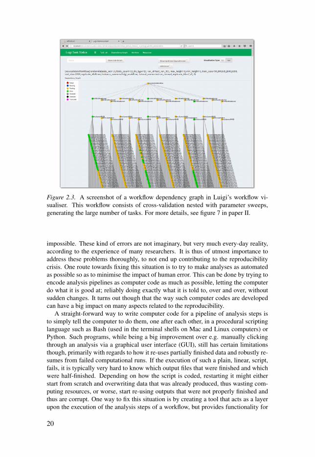
Figure 2.3. A screenshot of a workflow dependency graph in Luigi’s workflow vi-sualiser. This workflow consists of cross-validation nested with parameter sweeps,generating the large number of tasks. For more details, see figure 7 in paper II.

impossible. These kind of errors are not imaginary, but very much every-day reality,according to the experience of many researchers. It is thus of utmost importance toaddress these problems thoroughly, to not end up contributing to the reproducibilitycrisis. One route towards fixing this situation is to try to make analyses as automatedas possible so as to minimise the impact of human error. This can be done by trying toencode analysis pipelines as computer code as much as possible, letting the computerdo what it is good at; reliably doing exactly what it is told to, over and over, withoutsudden changes. It turns out though that the way such computer codes are developedcan have a big impact on many aspects related to the reproducibility.

A straight-forward way to write computer code for a pipeline of analysis steps isto simply tell the computer to do them, one after each other, in a procedural scriptinglanguage such as Bash (used in the terminal shells on Mac and Linux computers) orPython. Such programs, while being a big improvement over e.g. manually clickingthrough an analysis via a graphical user interface (GUI), still has certain limitationsthough, primarily with regards to how it re-uses partially finished data and robustly re-sumes from failed computational runs. If the execution of such a plain, linear, script,fails, it is typically very hard to know which output files that were finished and whichwere half-finished. Depending on how the script is coded, restarting it might eitherstart from scratch and overwriting data that was already produced, thus wasting com-puting resources, or worse, start re-using outputs that were not properly finished andthus are corrupt. One way to fix this situation is by creating a tool that acts as a layerupon the execution of the analysis steps of a workflow, but provides functionality for

20

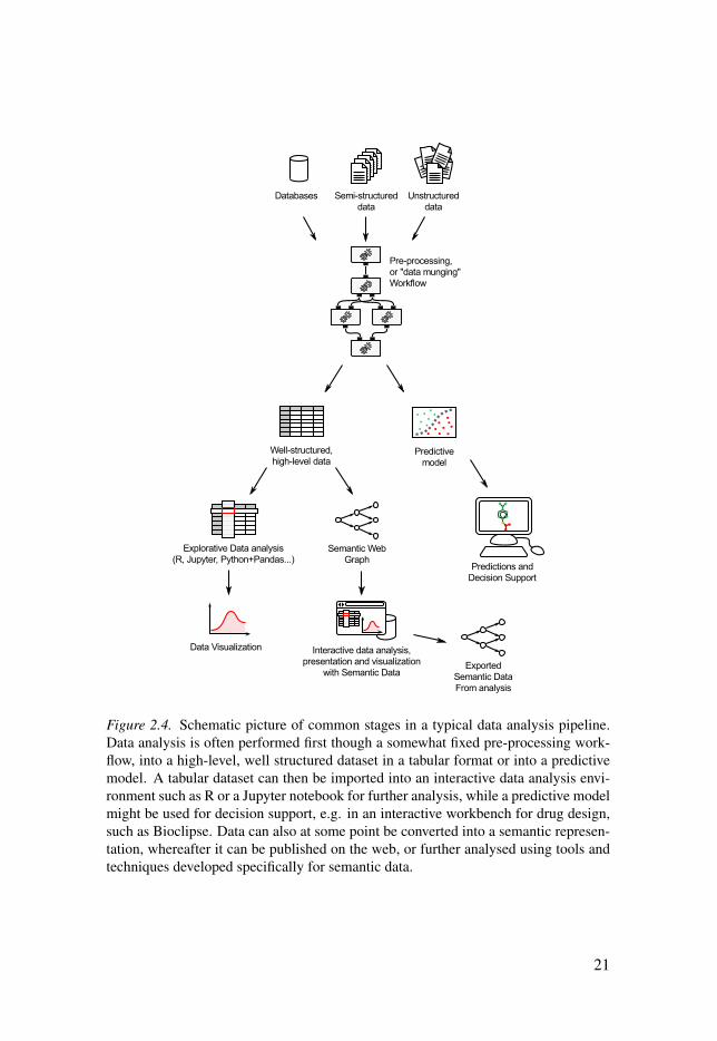
Figure 2.4. Schematic picture of common stages in a typical data analysis pipeline.Data analysis is often performed first though a somewhat fixed pre-processing work-flow, into a high-level, well structured dataset in a tabular format or into a predictivemodel. A tabular dataset can then be imported into an interactive data analysis envi-ronment such as R or a Jupyter notebook for further analysis, while a predictive modelmight be used for decision support, e.g. in an interactive workbench for drug design,such as Bioclipse. Data can also at some point be converted into a semantic represen-tation, whereafter it can be published on the web, or further analysed using tools andtechniques developed specifically for semantic data.

21

checking if existing data exists, and, while writing new results, keeping temporary out-put files separate from finished ones in order to make restarting an analysis safe andefficient. This is the job for a class of software tools often called Scientific WorkflowManagement Systems (SWMS), or simply workflow tools.

Numerous workflow tools have been developed in the past and it is outside of thescope of this thesis to provide a comprehensive review of all tools available. For tworecent reviews of a number of popular tools in bioinformatics, see [43, 44], and fora recent review reviewing a number of workflow tools in the context of reproducibleresearch, see [32].

The workflow tools developed vary widely in terms of focus, intended user baseand subsequent selection of features. To give a taste of these differences while alsointroducing some terminology, we will below briefly mention some representativeworkflow tools which are used in bioinformatics and contrast their differences. Verybroadly, one way of dividing the tools into multiple categories could be the follow-ing: GUI tools versus text-based tools, client/server based installations versus user-managed tools. Among GUI-tools one could divide between tools providing its GUIvia a web-server and those providing a native desktop interface. Among text-basedtools one can further divide the tools into those using their workflow description ina specialised, declarative text-format such YAML, those with a domain-specific lan-guage (DSL) and those implemented as programming libraries in existing, establishedprogramming languages.

Examples of GUI tools include Taverna [45], Galaxy [46, 47, 48, 49] and Yabi [50].While Taverna provides a native desktop interface, Galaxy and Yabi provide web-interfaces. Furthermore, dividing into client/server respective user-managed tools,Taverna falls into the user-managed category while Galaxy and Yabi are meant to beinstalled in a server/client fashion. Examples of text-based tools are Snakemake [51],Bpipe [52], Nextflow [53], Luigi [54] and Cuneiform [55]. Snakemake, Bpipe, Nextflowand Cuneiform are all implemented as DSLs with varying level of expressivity orscripting support, while Luigi is implemented as a programming library in the Pythonprogramming language. GUI tools quite naturally provide a benefit especially forcomputationally novice users, as they hide away a lot of the underlying technologyand provide a user interface with controls specific to the task at hand. For highlycomplex computations though, the available GUIs might not be adequate for fullyproviding control and insight into how the computations are run, and expert users thusoften prefer text-based tools that provide more direct access to all the aspects of theunderlying analysis tools [29].

The core functionality of most workflow tools is to describe the dependencies be-tween computing components (sometimes referred to as tasks, processes or nodes) andtheir input- and output data. Worth noting is that some tools describe the dependenciesdirectly between the computing components, while leaving the routing of individualinputs and outputs to be handled explicitly by specialised code in the components.

2.8 Data management and integrationNot only is it important to reliably manage computations, to achieve verifiability. Howwe handle data is also equally – if not even more – important.

22

There are many challenges present in the handling of data in the life sciences. Oneof them is that it is common to need to integrate data from vastly different sources togain a comprehensive model or understanding of a biological system. This processof data integration can easily lead to problems, for example if meta data such as theexact meaning of data, and/or the full provenance information about how the data wascreated, is not accompanying it. This can lead to incorrect assumptions about how thedata was created or what it means, in turn leading to mis-interpretation and mis-useof it. A recent attempt at summarising the challenges and some recommendations forhow to tackle them, is provided in the description of the FAIR guiding principles forscientific data [56], where each letter in the FAIR acronym stands for a describingcharacteristic of well-managed data. F for findable, A for accessible, I for Interoper-able and R for Re-usable.

In terms of technology, the most widely proposed solution today for maintainingFAIR data, is a set of data formats and technologies commonly referred to as the Se-mantic Web [57]. It consists of the data format Resource Description Framework [58],the query language SPARQL [59], the ontology language Web Ontology Language(OWL) [60], among others. Accompanying these formats are a number or proposedprinciples for how to encode data so that it is readily interoperable (or linkable) withother data, commonly referred to as Linked Data (LD), or Linked Open Data (LOD).The principles of LD and LOD are often implemented using the technologies fromSemantic Web, but are not in fact strictly tied to a particular format. For example,they have recently also been implemented in more recent data formats such as JSON-LD [61].

For more details on the particular technologies mentioned, please see the methodssection. The basic principle of the technologies and approaches making up the Seman-tic Web and Linked Data fields though, is that they enable storing data in a uniform,machine-readable, serialisation format. This format is flexible and generic enough toallow both linking multiple datasets together by indicating which entities representthe same thing, and linking additional meta data to the original data using the sameunderlying serialisation format. This has important practical benefits as it allows tokeep information about the exact, original meaning of data and potentially provenanceinformation stored tightly associated with the data itself. LD and LOD has becauseof this been used as a foundation for a concrete exemplary implementations of theFAIR guiding principles, presented in [62]. There also exist a number of complemen-tary techniques and formats such as the ISA metadata tracking framework [63], whichis built around a three-layered model of Investigation, Study and Assay, to achieve aproper treatment of the various abstraction levels involved in scientific experiments,and the SciData [64] framework, which aims to be a generic description layer forscientific data stored in SciData-JSON, or converted into RDF.

In this thesis, a number of the mentioned technologies have been used to try toimprove the ways in which scientists handle data. More specifically, we have usedthe RDF framework and the accompanying SPARQL query language, and integratedthem with a user-friendly wiki environment as well as developed tools for publishinglarge data in RDF format on the web.

23

3. Aims

This thesis has followed three parallel, but sometimes tightly intertwined tracks ofresearch in the area of computer-aided research in drug discovery. These tracks havehad separate, slightly different immediate aims. At the same time, all are aiming tocontribute towards more reproducible, understandable and verifiable research in earlydrug discovery. In more detail, and with references to the papers in this thesis, theaims have been the following:

• a) Make use of the increasingly large datasets available, on properties such assolubility and adverse effects of drug-like compounds, to build predictive mod-els that can aid in the drug discovery process by indicating potential problemswith newly developed compounds as early as possible (Papers I and V).

• b) Find ways to enable agile and flexible development of data processing work-flows for machine learning in drug discovery and apply these methodologies inaim a) above (Papers II and VI).

• c) Develop practical ways to publish and work collaboratively with researchdata in machine-readable, linkable form, such that it can become a practicalpossibility for scientists in their day-to-day research activities (Papers III andIV).

The most separate of these tracks is c). An aim in this research has been to ulti-mately merge the approaches developed in a) and b) with the ones in c). That is, todevelop methodologies that can encompass reproducible and verifiable managementof computations and data in an integrated, coherent system. This has turned out to bea larger project than anticipated though, and is left as a suggestion for a future researchproject, as outlined in the future outlook section.

24

4. Methods

4.1 The Signature descriptorThe descriptor method used in the predictive modelling work in this thesis is the sig-natures descriptor [65]. It works by computing all possible signatures of lengths be-tween a minimum and a maximum value specified (counted in the length of chemicalconnections in the signatures) in the compound. This min/max-length of connectionsin the signatures is called the height. For example, if signatures of heights 0-3 arecreated, the list of signatures will contain signatures of everything from single atoms(connection length zero) up to signatures with four atoms, or three connections inlength. Figure 4.1 shows a simple example of calculating signatures of height 0-2 forethanol, which is a very simple molecule.

When creating datasets for machine learning, it is common to create one column inthe output dataset for each unique signature and indicates with a zero or one whethereach particular signature is present or not in the compound. Signatures have the ap-pealing property that they can be interpreted and visualised as substructures in chem-ical structures. This also means that information linked to the signature can be visu-alised, such as the extent with which different signatures are contributing to a predic-tion. An example of this is shown in figure 4.2, which is adapted from figure 5b inpaper V.

This particular way of building the training dataset thus creates extremely sparsematrices, with mostly just zeroes, but with occasional ones here and there. This sparsenature of the dataset affects which machine learning methods are suitable to use fortraining models on this data. So called Support Vector Machines is one method thatworks well with such sparse datasets.

4.2 Support Vector MachinesSupport Vector Machines (SVM) is one of the most widely known and applied ma-chine learning methods in use, and is based on a rather simple idea that in its simplestform can be understood visually.

In the simplest form, with a binary classification case and a 2-dimensional dataset(that is, a dataset where each data point is described by two numerical variables), wecould think of this dataset as a 2 dimensional plot, with one of the variables on thex-axis and one on the y-axis, and all of the data points represented as dots in the plot.

If we assume that the dots belong to two different classes (say, circles and crosses),and these are clustered into two clearly separable clusters, then we can say that SVMwould separate these clusters by drawing a straight line between the two clusters,such that the distance from the line to the points closest to the line, in each cluster, ismaximised. In other words, it tries to draw a line between the two clusters, that avoids

25

Figure 4.1. Signatures of height 0 to 2 for ethanol. Note that we are using implicithydrogens meaning that they are not included in the signatures. A molecular signatureis made up of atom signatures for all heavy atoms in the molecule. The height defineshow much of each atom’s neighbourhood is in cluded. Figure adapted from [66]

Figure 4.2. Colouring of whichparts of a molecule (here Terbu-taline, which is a bronchodilatorand tocolytic which is used e.g.to treat asthma) has contributedthe most to a prediction. Redcolour here indicates the centresof molecular fragments that con-tributed most to the larger class,while blue colour indicates centreof fragments contributing most tothe smaller class. See figure 5bin paper V for more details aboutthis figure.

26

Figure 4.3. Schematic picture of a linear SVM classifier. the crosses and circlesrepresent data points belonging to two different classes respectively. The x- and y-axes represent two variables, which are included in every data point. the solid linerepresents the separating hyper-plane (just a line in the 2-dimensional case) while thedotted lines show where the so called margin lines go, that is, the line(s) along whichthe closest data points to the hyper plane lie. a) shows a linearly completely separablecase, where one can draw a straight line that completely separates the crosses fromthe circles. b) shows a case where this is not possible, since a few of the crosses hasended up in the circles cluster and vice versa.

27

coming too close to any of the clusters, but instead stays at the maximum distance fromthem, while still passing between them. This is illustrated schematically in figure 4.3 a.For this kind of simple example where the classes can be 100% separated, we can havea very strict criteria that each dot needs to be in the right cluster – that is, stay closetogether to other dots of the same class, and not intermingle with dots of the otherclass. Such a classifier, where no exceptions from this rule is allowed, is called a hardmargin classifier.

It is quite uncommon to have such cleanly separated clusters though. Often, a fewdata points end up closer to the cluster of the other class, and vice versa. An exampleof this is shown schematically in figure 4.3 b. It is common to not be able to completelyseparate the clusters unless we introduce a bit of “slack” into the method, that allowsa certain number of points to break the rule of staying on the right side of the cluster.This is called a soft margin classifier and is commonly used in SVMs.

An even harder problem, is if the two clusters are arranged in such a way that wecan not even in principle separate them by drawing a straight line between them. Thiscould be the case e.g. if one of the classes form a ring around the other class’ cluster.Any way of drawing a straight line through such a plot would by necessity get dotsof both classes on both sides of the “separating” line. Thus, we need to do somethingsmarter to separate classes in that case.

The solution to this problem that is commonly employed in SVM, is to apply atransformation to the dataset, that creates a dataset with more dimensions, For exam-ple, our 2-dimensional “plot”, could become a 3-dimensional one, by adding a heightto each dot as well. Then, depending on what transformation function we use, if weare lucky, there might be a way to form a linear separating plane (it is not enoughwith a line to separate clusters in three dimensions), through this 3D space. After wehave found such a separating plane, we can then use the reverse of the transforma-tion function we used earlier to go back to our 2D-plot. The separating plane that wefound, will no longer be a straight line when transformed back to the 2D-form, butthat doesn’t matter, as long as we found a way to separate the clusters and that wecould re-use the same simple principle as in the simple, linear case described above.This way of transforming a dataset to a higher-dimensional form before finding a sep-arating (hyper-)plane, is called the kernel trick. In this thesis, we have used both alinear implementation of SVM, as well as SVM with the radial basis function (RBF)kernel. Both of these have a parameter called cost, which needs to be optimised beforethe training. The RBF kernel is a very commonly used one and has the benefit thatso called radial basis functions can easily be combined to create very complex andnon-linear while still smooth decision boundaries. The RBF kernel has an additionalparameter, γ , that needs optimisation before training.

For a brief, but slightly longer, explanation of SVMs, see [67].

4.3 Conformal PredictionA problem with traditional machine learning methods, including Support Vector Ma-chines, is that they lack measures of confidence of their predictions. In other words,they don’t provide information about how reliable a particular prediction is for a newobject. The most common approach to address this has been to provide estimates

28

of predictive accuracy based on an external test set or cross validation, with the as-sumption that these estimates are relevant for future predictions. However the un-certainty on how different new examples are from the examples used to estimate theperformance has lead to research on how to define the applicability domain of models.Several methods have been proposed to define such measures but have not generallymanaged to achieve mathematically guaranteed levels of confidence in the predictions.

Conformal Prediction (CP) [68] is a method that aims to address this by comple-menting existing machine learning methods such as Support Vector Machines, Ran-dom Forest and Neural Networks with a mathematical framework that generates pre-diction intervals with guaranteed validity as outcome. In the case of regression, thiscomes as an interval around the predicted midpoint. In the classification case, we getseparate so called p-values1 for each label, indicating how probable it is the true label.This is explained in more detail below.

CP was initially implemented for on-line training in what is called transductive con-formal prediction (TCP). This is a very computationally resource demanding methodthough, which is why we are in this thesis using the inductive conformal prediction(ICP) method instead. The process of training and predicting models with ICP isbriefly covered below.

In ICP, the dataset is first split into a proper training-, and a calibration dataset. Theway to split up the dataset can differ. In this thesis we have used Cross-ConformalPrediction which works similarly to cross-validation, using the whole training datasetboth for training and calibration. After the splitting is done, a model is trained on theproper training set. Using this model a non-conformity measure is calculated for eachof the examples in the calibration set. The choice of nonconformity measure can varywidely. In this thesis, since we are using Support Vector Machines as the underlyingmachine learning method, we use a nonconformity measure based on the example’sdistance from the decision plane in the SVM model. The obtained values, the so callednonconformity scores, α , are then stored in one list per label. Later, in the predictionstep, given a new object, we compute the same type of non-conformity score α for it.We then compare this value, α , with the lists of α for each label which were producedearlier. Based on the comparison with the lists, p-values2 are calculated for each labelas the fraction of examples with that label that have a lower non-conformity score α

than the new object. In other words, a high p-value means that the new object is moreconforming than many of the examples used in the calibration, thus indicating that thenew object could be belonging to this label. Because we get, for every new object,separate p-values for each label, we can select a confidence level which is used as athreshold for which p-values to accept. This means that based on the p-values we get,and the confidence level we choose, we might end up with either one of the labels,both of them, or none which make it over the confidence threshold. If none or bothlabels make it above our threshold, this means that a prediction could not be madeat the selected confidence level. Conversely, if only one of the labels’ p-values makeit above the threshold, this results in a prediction that the new object belongs to thatlabel.

CP has the (very attractive) property that predictions are always guaranteed to bevalid, where valid means that the rate of erroneous predictions will be the same as the

1Not to be confused with traditional p-values from statistics2Again, not to be confused with traditional p-values from statistics

29

error rate ε , given a confidence level given as 1− ε . This guarantee holds under theso exchangeability assumption, meaning that training examples are not following anyparticular order.

Because validity is guaranteed in CP, we are focusing mainly on maximising ef-ficiency, when training models. Efficiency is in the regression setting a measure ofthe width of the prediction interval, and thus says something about how exactly wecan predict a value. Note that somewhat unintuitively, efficiency is defined in such away that a small prediction interval (thus a more exact prediction), is giving a smallerefficiency value. In other words, we want to minimise the efficiency value, althoughit might have been more intuitive to think about it as maximising the exactness ofpredictions. In the binary classification setting, efficiency can e.g. be calculated asa fraction of double-label predictions achieved. That is, the smaller this efficiencyvalue is, the more often we can achieve a single label and thus make a prediction. Forclassification, there are alternative efficiency measures though, and we explore a fewalternatives in paper V.

For a generic introduction to conformal prediction, see [69], and for an introductionto conformal prediction in cheminformatics, see [70].

4.4 Flow-based programmingFlow-Based Programming (FBP) [71] is a programming paradigm developed at IBMin the late 60s / early 70s, to provide a composable way to build up computations tobe run at mainframe computers at customers such as large banks.

The main ideas of the paradigm is to divide a program into independent and asyn-chronously running processing units called processes, which are allowed to commu-nicate with other processes only via message passing over channels with boundedbuffers, connected to named ports on the processes. Importantly, the network of pro-cesses and channels is in FBP kept separate from the process implementations.

This strict separation of the network structure from processing units and the loosely-coupled nature of its only way of communication, makes flow-based programs verycomponent-oriented and also very composable. The network can be re-wired end-lessly without changing the internals of processes, and any process can always bereplaced with any other process that supports the same format of the data packets onits in-ports and out-ports. This makes it easy to plug in analysis components such asloggers, testing components and various analysers at any place in the network. Thecomponent-based nature, and the fact that the connectivity graph of FBP programsare handled separately, makes FBP suitable for integration with visual programmingenvironments, as well as makes it natural to manually or automatically create visuali-sations of the program structure. Figure 4.4 shows the program structure (connectivitynetwork) for the rdf2smw tool, which was developed as part of paper III, created withthe drawfbp software.

Since the processes are allowed to run asynchronously, FBP is very well suited tobe run on multi-core CPUs, where each processing unit can suitably be placed in itsown thread or co-routine, and spread out on the available CPU-cores on the computer.

The fact that processes only communicate via message passing, means that the oth-erwise very common race conditions in threaded versions of procedural programs do

30

Figure 4.4. Flow-based programming di-agram, drawn with the drawfbp soft-ware, showing the connection graph of therdf2smw tool which was developed as partof paper III in this thesis. Boxes represent(asynchronously running) processes, whilearrows represent data connections, whichare in FBP implemented as channels withbounded buffers. The names at the headsand tails of arrows, represent named out-and in-ports respectively.

not generally occur at all. Instead, the buffered channels provide the synchronisationmechanism needed for handing off work from one thread to another (if assuming thateach process runs in its own thread).

FBP has a natural connection to workflow systems, where the computing networkin an FBP program can be likened to the network of dependencies between data andprocessing components in a workflow [72].

FBP also has striking similarities with another programming approach, called Com-municating Sequential Processes (CSP) [73], on which the concurrency primitives inthe Go programming language are built. Just like in FBP, CSP programs are basedupon asynchronously running processes (in Go represented by go-routines), whichcommunicate solely via message passing on channels. In CSP, channels are by de-fault unbuffered, but buffered channels are allowed in Go, making it very similar toFBP channels. What is missing from CSP are primarily the ideas of separate networkdefinition between named ports bound to process objects. These can easily be addedin Go though, by encapsulating go-routines in structs with named fields referencingchannels, to constitute the ports. This is the underlying principle upon which theSciPipe workflow system is built, which is described in paper VI.

4.5 RDFThe Resource Description Framework (RDF) [58], is a framework for representingknowledge in the form of a graph, where nodes represent so called resources (whichrepresent any kind of “thing”), and are identified either by so called Uniform Re-source Identifiers (URIs), for resources which are further linked to other resources,

31

Figure 4.5. An example of data in the form of RDF triples of subject, predicate andobject, together forming a graph of resources linked with predicates. The example isfrom a dataset of NMR spectra for molecules, as described in [74]. In plain English,the figure says that the molecule has a spectrum, which has a number of peaks, eachwith a shift value, which is a numerical value.

or literal values, for storing simple values such as numbers or strings. The edges thatlink resources together are called predicates, and are themselves also in fact resources,meaning that they can also be linked to resources that describe them. An illustrationof the graph nature of data in RDF, is shown in figure 4.5, which shows an examplefrom a dataset containing NMR spectra which describe molecules, where each spec-trum contains a set of peaks, which each has a shift value. The dataset used for theillustration is further described in [74].

RDF comes in a few different serialisations or concrete textual data formats. Themost commonly used of these are RDF/XML, Turtle and N-triples. While RDF/XMLrepresent the graph with a nested XML hierarchy, most other formats represent thegraph in form of triples, of the form Subject - Predicate - Object, where theSubject and Predicate are always URIs, while the object can be either URIs or literals.

A recent new format, RDF-HDT [75, 76], stores RDF data in a much more compactway than the text-based formats mentioned above. HDT stands for "Header, Dictio-nary, Triples", and reflects the basic structure of the format. It is a binary format thatprovides a search index (represented by the “Dictionary” part in the name), that allowslooking up facts quickly despite the compact binary representation.

The fact that all data in RDF is described in a graph form, where the predicates canbe seen both as edges linking resources together, but are also themselves resources,means that it is possible to add meta data also about the predicates, such as telling thattwo properties from two different ontologies mean the same thing (this can be donee.g. with the owl:sameAs predicate from the OWL ontology). This ability of RDF

32

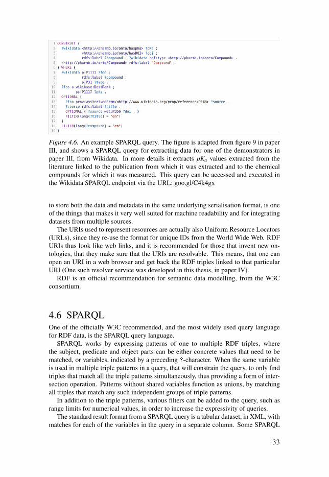
Figure 4.6. An example SPARQL query. The figure is adapted from figure 9 in paperIII, and shows a SPARQL query for extracting data for one of the demonstrators inpaper III, from Wikidata. In more details it extracts pKa values extracted from theliterature linked to the publication from which it was extracted and to the chemicalcompounds for which it was measured. This query can be accessed and executed inthe Wikidata SPARQL endpoint via the URL: goo.gl/C4k4gx

to store both the data and metadata in the same underlying serialisation format, is oneof the things that makes it very well suited for machine readability and for integratingdatasets from multiple sources.

The URIs used to represent resources are actually also Uniform Resource Locators(URLs), since they re-use the format for unique IDs from the World Wide Web. RDFURIs thus look like web links, and it is recommended for those that invent new on-tologies, that they make sure that the URIs are resolvable. This means, that one canopen an URI in a web browser and get back the RDF triples linked to that particularURI (One such resolver service was developed in this thesis, in paper IV).

RDF is an official recommendation for semantic data modelling, from the W3Cconsortium.

4.6 SPARQLOne of the officially W3C recommended, and the most widely used query languagefor RDF data, is the SPARQL query language.

SPARQL works by expressing patterns of one to multiple RDF triples, wherethe subject, predicate and object parts can be either concrete values that need to bematched, or variables, indicated by a preceding ?-character. When the same variableis used in multiple triple patterns in a query, that will constrain the query, to only findtriples that match all the triple patterns simultaneously, thus providing a form of inter-section operation. Patterns without shared variables function as unions, by matchingall triples that match any such independent groups of triple patterns.

In addition to the triple patterns, various filters can be added to the query, such asrange limits for numerical values, in order to increase the expressivity of queries.

The standard result format from a SPARQL query is a tabular dataset, in XML, withmatches for each of the variables in the query in a separate column. Some SPARQL

33

Figure 4.7. A screenshot of a wiki page in Semantic MediaWiki. The informationshown is automatically gathered from the structured data in SMW (which was im-ported using RDFIO) using an SMW ASK query, and presented using MediaWikitemplates. The figure is adapted from figure 8 in paper III,

engines also support a special CONSTRUCT keyword, which allows constructing andreturning new RDF triples, based on matches from the query. The CONSTRUCT clauseallows customising how these new triples are formed, using a triple pattern syntaxsimilar to the one for the query part. An example SPARQL query, including withthe CONSTRUCT keyword, can be seen in figure 4.6, which is adapted from figure 9 inpaper III.

4.7 Semantic MediaWikiSemantic MediaWiki (SMW) [77] is an extension for MediaWiki, the software thatpowers Wikipedia, and thousands of other wiki-based websites, small and large, bothwithin the Wikimedia organisation and outside.

SMW extends the wiki syntax of MediaWiki with ability to tag wiki pages withfacts on the form of [[property::value]]. The page itself serves as the subject.The facts in SMW thus closely map to the subject-predicate-objects triples in the RDFdata model.

The properties used in SMW facts are themselves represented by specific wikipages under a special namespace. On these pages, the properties can be taggedwith special-purpose facts to provide more information about their data type, allowedranges and more.

The value part of SMW facts can be either references to other wiki pages (refer-enced by their name in the main wiki namespace), or literal values. These two casesmap closely to triples linking to URIs and literals, respectively, in RDF. Which type aparticular fact is referring to, can be defined on the wiki’s property page for the prop-

34

erty used in the fact. Each property always is either of “Page” type (linking to otherwiki pages) or of a literal value type, such as text or number.

SMW comes with its own built-in query language, called ASK [78], that allowspresenting data added as facts in tabular formats, with usual controls such as sortingand filtering.

SMW facts can be used together with the powerful templating system [79] in Me-diaWiki to provide automatic tagging of articles with facts according to pre-definedpatterns, based on parameters sent to templates. The same information can then beused to parse such parameters into easy to use presentations of data, using tables andvisualisations. ASK queries can also be used to pull in data related to a particularpage, in the presentation on that page. These capabilities were employed in the casestudies for the RDFIO tool suite in paper III. A page where MediaWiki templates andan SMW ASK query was used to automatically format and summarise data is shownin figure 4.7, which is adapted from figure 8 in paper III.

Facts entered in an SMW wiki are available as RDF via a built-in RDF exportfeature. SMW does not come with a built-in RDF import function though. It providesa feature for defining a mapping from property pages to URIs in an ontology, providingsomething called vocabulary import [80], but does not allow importing plain RDFtriples (the same as OWL individuals).

This lack of plain triples RDF import was the motivation for developing the RDFIOsuite of tools presented in paper III.

35

5. Results and Discussion

5.1 Balancing model size and predictive performance inligand-based predictive modelling

In paper I, we studied the effect of dataset (and resulting model-) size on the predic-tive performance and modelling (training) time of predictive models. Models werebuilt using two implementations of Support Vector Machines (SVM). We used bothlibSVM with the radial basis function (RBF) kernel and the LIBLINEAR linear SVMimplementation. Chemicals were described using the signatures molecular descrip-tor [65], and the biological activity studied was solubility and a molecular propertycalled LogD or distribution coefficient, which gives information about the hydropho-bicity of a compound and is experimentally measured as its partitioning between anoctanol and water mixture [9].

The results from this study showed that SVM with the RBF kernel (SVM RBF)was unfeasible for large datasets due to the very large computing requirements. Eventhough we used the parallel version of SVM with multi-node jobs, using four computenodes with 64 computing cores in total, the largest datasets would require more thanseven days to train. Such large training times mean that the risk for a break in thecomputation because of a temporary network outage or the need to patch the operatingsystem for security vulnerabilities increases dramatically. Such long training timesalso can hinder an iterative, exploratory mode of working, since researchers might notbe able to progress further with a project until the training has finished.

The SVM LIBLINEAR implementation on the other hand, mostly outperformedSVM RBF in terms of performance per modelling time. For large datasets, one couldget very good results despite a negligible training time compared to SVM RBF. Basedon this finding, the Bioclipse decision support framework was extended with supportfor LIBLINEAR models, and the models resulting from this work were made availablethrough Bioclipse. Based on these results, we draw the conclusion that LIBLINEAR isa suitable modelling method for large QSAR datasets as it allows to include as muchtraining data as possible without getting impractical training times. SVM RBF canstill be preferable when the available data is limited, such that the training time willnot be too long anyway. For such cases SVM RBF will provide a slight improvementin predictive performance over LIBLINEAR.

5.2 Predicting target binding profiles with conformalprediction

Understanding how a drug candidate interacts with the proteome of the human bodyis of vital importance in the drug development process. This is because it is important

36

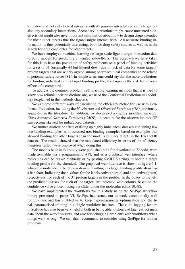
to understand not only how it interacts with its primary intended (protein) target butalso any secondary interactions. Secondary interactions might cause unwanted side-effects but might also give important information about how to design drugs intendedfor those other targets that the ligand might interact with. All accurate binding in-formation is thus potentially interesting, both for drug safety studies as well as in thesearch for drug candidates for other targets.

We have employed machine learning on large-scale ligand-target interaction datato build models for predicting unwanted side-effects. The approach we have takenfor this is to base the prediction of safety problems on a panel of binding activitiesfor a set of 31 (originally 44 but filtered down due to lack of data for some targets)protein targets that are widely agreed among pharmaceutical companies to be relatedto potential safety issues [81]. In simple terms one could say that the more predictionsfor binding indicated in this target binding profile, the larger is the risk for adverseeffects of a compound.

To address the common problem with machine learning methods that it is hard toknow how reliable their predictions are, we used the Conformal Prediction methodol-ogy (explained in the methods chapter).

We explored different ways of calculating the efficiency metric for use with Con-formal Prediction, including the M criterion and Observed Fuzziness (OF), previouslysuggested in the literature. In addition, we developed a sligthly modified measure,Class-Averaged Observed Fuzziness (CAOF), to account for the observation that OFcan become skewed for imbalanced datasets.

We further studied the effect of filling up highly imbalanced datasets containing fewnon-binding examples, with assumed non-binding examples based on examples thatshowed binding for other targets than for model’s primary target, in the ExcapeDBdataset. The results showed that the calculated efficiency in terms of the efficiencymeasures tested, were improved when doing this.

The models built in this study were published both for download on Zenodo, weremade available via a programmatic API, and as a graphical web interface, wheremolecules can be drawn manually or by pasting SMILES strings to obtain a targetbinding profile for the chemical. The graphical web interface is shown in figure 5.1,where the molecule Terbutaline is drawn, resulting in a target binding profile shown asa bar chart, indicating the p-values for the labels active (purple) and non-active (green)respectively, for each of the 31 protein targets in the profile. In the boxes to the left,the predicted classes for each of the targets are indicated with colours, based on theconfidence value chosen, using the slider under the molecular editor (0.48).

We have implemented the workflows for this study using the SciPipe workflowlibrary presented in paper VI. SciPipe has turned out to work exceptionally wellfor this task and has enabled us to keep hyper-parameter optimisation and the fi-nal, parametrised training in a single workflow instance. The audit logging featurein SciPipe has also been very helpful both in being able to store and later extract metadata about the workflow runs, and also for debugging problems with workflows whenthings went wrong. We can thus recommend to consider using SciPipe for similarproblems.

37

Figure 5.1. The graphical web interface for predicting target binding profiles. Inthe molecular editor, the structure for Terbutaline has been drawn. To the right, the p-values for the targets in the profile are shown as a bar chart, with purple bars indicatingthe p-values for the binding label, and green bars the p-values for the non-bindinglabel. In the slider under the molecular editor, the confidence level has been set to0.48, which resulted in the discrete predictions of labels, shown as background colorsin the boxes with target protein names, below the slider.

38

5.3 Enabling development of complex workflows inmachine learning for drug discovery

5.3.1 Agile machine learning workflows based on Luigi withSciLuigi

In paper II, we developed an approach which enables using the Luigi workflow frame-work [54], developed by Spotify AB, to develop complex scientific workflows in anagile way.

Luigi’s API is optimised for fixed workflow connectivity, with mainly varying pa-rameter values. This design is not a great fit for workflows which need constant, itera-tive rewiring, during the exploratory phase of a research project. We thus developed analternative API on top of Luigi, which uses certain design principles from Flow-BasedProgramming (FBP) to enable flexible and composable workflow connectivity.

The improved API has been released as open source software in the form of alibrary, called SciLuigi (github.com/pharmbio/sciluigi).

In more details, the following improvements are provided in the SciLuigi library.Firstly, dependencies are defined between the data inputs and outputs of tasks ratherthan between tasks directly. This enables to keep the dependency graph definitioncompletely separate from task definitions. Separate network definition is a core prin-ciple in Flow-based programming, which provided inspiration for this improvement.

The improvements provided by SciLuigi have turned out to greatly enhance theability to develop complex workflows for machine learning in drug discovery, as de-scribed in an accompanying case study. Some workflow constructs that we were un-able to create with vanilla Luigi, were relatively straight-forward to create in SciLuigi.

In addition, some functionality commonly required in scientific workflows, butwhich was not included in the core Luigi library, were added, including audit log-ging of executed tasks, execution times and more. Support for the SLURM resourcemanager [82] was also added.

5.3.2 Flexible, dynamic and robust machine learning workflowsin the Go language with SciPipe

In Paper VI, we developed the SciPipe workflow programming library, based on ex-periences in previous work and problems identified in existing workflow tools.

Some of the frustrations we experienced with Luigi and SciLuigi was that no morethan 64 concurrent workers could be started on the same compute node, even if theywere just idling and waiting for a remote HPC cluster job to complete. Another prob-lem was that because of the interpreted nature of Python, a workflow could fail far intoa many-day HPC job, because of a simple error such as KeyNotFound. These weresome of the reasons for why we started exploring other options.

At some point we realised that the job that Luigi was doing with a rather complexPython code base, could actually be replaced with a very simple scheduling mecha-nism based on dataflow and Flow-based programming approaches, implemented usingthe concurrency features in Go.

39

Very briefly, SciPipe uses the concurrency features in Go (go-routines and bufferedchannels) to create a network of processes and channels, that can be loosely likenedwith a factory with processing stations connected with conveyor belts.

Packets, in this case representing data files, would travel over the conveyor belts(buffered channels) until they reach processing stations which would use the contentsof the package, process it, and put back updated content into a new packet which issent over another conveyor belt, to another process.

With this approach, it turns out that we don’t need a central scheduler process. In-stead we can allow the asynchronously and independently running processes to sched-ule tasks (operations on packets) independently, based on in-coming packets.

We can still have some global rules, such that only a particular number of processesare allowed to process a packet at any given time (a given number of concurrent tasksto execute in the system), in order not to over-book computational resources but thisapproach still turns out to result in a much simpler system than with a central schedulerprocess implemented with procedural code. This is manifested by the fact that theSciPipe code base, with around 1500 lines of code, is considerably smaller than formany other workflow systems [83].

The conveyor-belt factory-like approach to workflow execution also means thatSciPipe allows dynamic scheduling. That is, tasks can be scheduled during the work-flow run and thus be parametrised and scheduled based on results obtained during theworkflow run. This has turned out to be highly relevant for workflows in machinelearning where it is common to first optimise one or more hyperparameters as partof the workflow, and based on the optimised parameter value(s) parametrise and ini-tiate the final training, as the last part of the workflow. This was not easily done inLuigi/SciLuigi where instead we had to start a completely new Luigi instance from thefirst part of the workflow (the part that did the parameter optimisation) so that it couldbe parametrized with optimised parameters. This had a number of problem resultingfrom the need to manage multiple Luigi instances such as fragmented audit logs andeven larger problems with resource usage.

While some workflow tools, in particular Nextflow, also offer dynamic scheduling,SciPipe additionally allows creating re-usable components that can be incorporated innew workflows on-demand, which has been a core requirement in our work towardsagile workflow design in drug discovery.

SciPipe also provides a state-of-the art system for audit logging, that creates self-contained audit logs for every output file from workflows, in the structured JSONformat. These can be converted to reports in HTML or PDF format, or into executableBash scripts using converter tools available in a command-line helper tool. SciPipealso provides a function for exporting the workflow dependency graph in the GraphVizDOT format, or as a PDF image. An example of such a graph is shown in figure 5.2,which represents the genomics demonstrator workflow in paper VI.

The fact that SciPipe is implemented in the statically typed, linked and compiledGo programming language, means that SciPipe solves the performance problems wefaced earlier with Luigi and SciLuigi. It also means that workflows can be compiledinto self-contained executable files, which make the deployment of SciPipe workflowsvery easy.

40

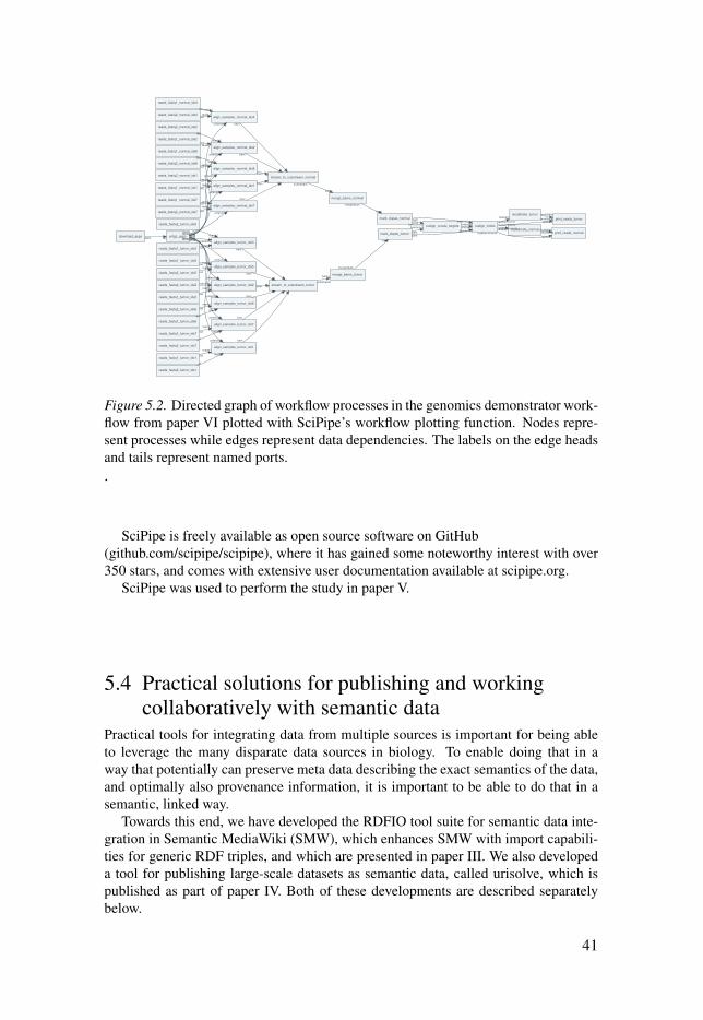
reads_fastq2_normal_idx4align_samples_normal_idx4

reads2out

reads_fastq1_tumor_idx6

align_samples_tumor_idx6

reads1

out

stream_to_substream_tumor

in

bam

realign_create_targets realign_indelsintervalsintervals

align_samples_tumor_idx7

in

bam

merge_bams_tumor

mark_dupes_tumor

bam

mergedbam

recalibrate_tumorprint_reads_tumorrecaltable

recaltable

align_samples_normal_idx1

stream_to_substream_normal

inbam

reads_fastq1_normal_idx2

align_samples_normal_idx2reads1out

reads_fastq2_normal_idx7

align_samples_normal_idx7reads2

out

reads_fastq2_tumor_idx5

align_samples_tumor_idx5reads2

out

reads_fastq1_normal_idx4

reads1out

reads_fastq2_tumor_idx1

align_samples_tumor_idx1

reads2

out

reads_fastq2_tumor_idx3

align_samples_tumor_idx3

reads2

out

reads_fastq2_tumor_idx7

reads2

out

mark_dupes_normal

bamnormalbam

bamnormalbam

reads_fastq1_tumor_idx1

reads1

out

in

bam

in

bam

download_apps untgz_appstgzapps

reads_fastq2_normal_idx2

reads2

out

in

bam

reads_fastq2_normal_idx8

align_samples_normal_idx8reads2out

in

bam

bamtumor

bam bamtumor

bam

untardone

done

untardone

done

untardone

done

untardone

doneuntardone

done

untardone

done

untardone

done

align_samples_tumor_idx2

untardone

done

untardone

done

untardone

done

untardone

done

recalibrate_normalprint_reads_normal

recaltablerecaltable

bams

substream

reads_fastq1_tumor_idx2

reads1

out

inbam

reads_fastq1_tumor_idx3reads1out

merge_bams_normal

bams

substream

in

bam

reads_fastq1_normal_idx8

reads1out

bam

mergedbam

reads_fastq2_tumor_idx6

reads2

out

reads_fastq1_tumor_idx7

reads1

out

realbam

realbamtumor realbamrealbamtumor

realbamrealbamnormal

realbam

realbamnormal

in

bam

reads_fastq1_normal_idx7reads1out

inbam

reads_fastq1_tumor_idx5reads1

out

reads_fastq1_normal_idx1reads1out

reads_fastq2_normal_idx1reads2out

reads_fastq2_tumor_idx2 reads2out

Figure 5.2. Directed graph of workflow processes in the genomics demonstrator work-flow from paper VI plotted with SciPipe’s workflow plotting function. Nodes repre-sent processes while edges represent data dependencies. The labels on the edge headsand tails represent named ports..

SciPipe is freely available as open source software on GitHub(github.com/scipipe/scipipe), where it has gained some noteworthy interest with over350 stars, and comes with extensive user documentation available at scipipe.org.

SciPipe was used to perform the study in paper V.

5.4 Practical solutions for publishing and workingcollaboratively with semantic data

Practical tools for integrating data from multiple sources is important for being ableto leverage the many disparate data sources in biology. To enable doing that in away that potentially can preserve meta data describing the exact semantics of the data,and optimally also provenance information, it is important to be able to do that in asemantic, linked way.

Towards this end, we have developed the RDFIO tool suite for semantic data inte-gration in Semantic MediaWiki (SMW), which enhances SMW with import capabili-ties for generic RDF triples, and which are presented in paper III. We also developeda tool for publishing large-scale datasets as semantic data, called urisolve, which ispublished as part of paper IV. Both of these developments are described separatelybelow.

41

5.4.1 Enabling collaborative editing of semantic data in auser-friendly environment with RDFIO

Previous efforts at creating import functionality in SMW have focused on using on-tologies to bootstrap a wiki structure, but has lacked support for the plain RDF triples(OWL individuals). RDFIO goes further than these earlier approaches by allowingimport of plain RDF data, without requiring an explicit ontology definition for it. Itdoes, however, also use a best-effort strategy for identifying classes and other ontologystructure in the data, where such can be found.

The RDFIO tool suite consists of two main parts: i) The RDFIO MediaWiki/SMWplugin (referred to as the RDFIO plugin) and ii) the stand-alone rdf2smw tool (re-ferred to as rdf2smw). While RDFIO is a PHP-based plugin for Semantic MediaWiki,which exposes its functionality via web forms available inside the MediaWiki soft-ware, the rdf2smw tool is a separate, command-line tool written in Go for improvedperformance.

In principle, these two tools take almost the exact same approach to how to con-vert from RDF to MediaWiki pages, including selection of suitable wiki page titles.Technically though, they do differ in how they go about the conversion: While theRDFIO plugin does the import page by page, straight into the MediaWiki database,the rdf2smw tool “just” converts the RDF data into a MediaWiki XML dump file, forfurther batch import using MediaWiki’s built-in XML import feature (also a batchcommand-line script). Our experiences show that the rdf2smw tool is more scalableand practical to use for very large datasets, while the RDFIO plugin is more userfriendly because of its web interface, and thus might be preferred for smaller datasets, or for end-users not used to the command-line. Using the rdf2smw tool, we havesuccessfully imported datasets in the order of 0.5 million RDF triples, into SemanticMediaWiki.

Building on the user-friendliness and familiarity of wiki systems and MediaWikiin particular, the RDFIO solution turns SMW into a viable solution for a number ofuse case scenarios in data integration, such as bootstrapping a wiki structure from anexisting dataset, collaboratively creating mash-ups of data from multiple data sourcesenhanced by the summarising and visualisation capabilities already present in SMW,or by replicating an existing semantic data store exposed via a SPARQL endpoint (viathe SPARQL endpoint replication feature, and then exposed via the built-in SPARQLendpoint in the RDFIO plugin). A selection of these possible use cases are demon-strated by demonstrators in the paper. An overview of the developed functionality inthe RDFIO tool suite is shown in figure 5.3.

The RDFIO suite of tools are released as open source code and available for down-load from the rdfio GitHub organisation: github.com/rdfio

5.4.2 Publishing large-scale semantic datasets on the webA common problem with current serialisations for semantic data in RDF is that be-cause of the disaggregated nature of the triple-based way of representing knowledgegraphs, it is common that a full RDF data file needs to be read into memory in orderto do lookups and integrate the pieces of the graph.

42

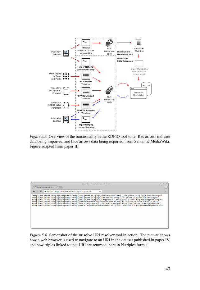
Figure 5.3. Overview of the functionality in the RDFIO tool suite. Red arrows indicatedata being imported, and blue arrows data being exported, from Semantic MediaWiki.Figure adapted from paper III.

Figure 5.4. Screenshot of the urisolve URI resolver tool in action. The picture showshow a web browser is used to navigate to an URI in the dataset published in paper IV,and how triples linked to that URI are returned, here in N-triples format.

43

While such interactive lookup and querying of RDF datasets can be done efficientlyusing semantic databases, so called triple stores, the intended role for RDF has grownto be more than a format for exposing databases. It has turned into a general exchangeformat for data on the web [76]. It is also not always practical to install and run triplestores everywhere data in semantic form need to be managed. There are thus strongincentives for better and simpler ways to manage RDF data.

One way to do this is via the RDF-HDT format [75, 76], which is described inmore details in the methods chapter. The RDF-HDT format provides an efficient whileflexible way to store and access RDF data, by using a combination of a compact binarystorage format, with an index to allow quick on-demand lookups of specific data.

In paper IV, in addition to training and publishing a predictive model for predictinglogD values, we also used the model to predict logD for 91 million chemical structuresfrom PubChem. This resulted in a large dataset that we have made available as an RDFdata file for download.

To make the newly created dataset follow best practice guidelines, all newly mintedURIs should be dereferencable such that navigating to a URI in a web browser shouldreturn the triples linked to that particular URI. This can raise challenges with largedatasets though, as really large datasets are not trivial to publish as web services.Even just the compressed downloadable dataset developed in paper IV, is 4.5 Gb insize.

To enable making newly minted URIs in the dataset described above, we developeda simple URI resolver tool, called urisolve, which uses the RDF-HDT C++ library tolook up the relevant triples for a URI in question, and returns those to the user. The toolis written in Go, is available as open source software at github.com/pharmbio/urisolve.A screenshot of the tool in action for the dataset in paper IV, is shown in figure 5.4.

5.5 Lessons learnedDuring this thesis, a number of lessons have been learned, that are of a more over-arching nature than the individual results from the studies and research papers. Thesewill be briefly discussed below.

5.5.1 Importance of automation and machine-readabilityOne fact that is almost too obvious, but at the same time not always exploited toits full potential in practice, is that automation will increase reliability in computer-aided research. That is, the main motivation for using computers in research at all, isbased on the fact that computers shine in an area where humans are not excelling: atperforming repetitive, mundane tasks with maximum precision and reliability. Today’scomputers are reliable to the point where we can generally count on them to properlydo what they are told. If there is an error in a calculation, that is almost always thefault of the user, or the programmer who created the program that was in use1. Thus,

1It is important to note that there are in fact limits even to computational reliability. In particularwith very large scale storage and computations, the sheer scale of operations increases thestatistical chance that errors do occur, to an extent that it actually needs to be handled. It is thus

44

it will generally pay off to make use of this strength of computers, and try to automateas much as possible.

It is also true that definitely not everything a researcher does is automatable, orshould be automated. There is always a part of research that follows a more ex-ploratory pattern, and thus needs to be done in an interactive way.

One way to address this duality between interactiveness and automation, is to tryand use tools that can automate certain aspects of analyses, while still allowing thecore logic of an analysis to be implemented interactively. There have been someinteresting explorations in this space, such as the noWorkflow tool, which can cap-ture provenance based on simple Python scripts, even without using a workflow sys-tem [84].

Another way can be to make the tools we use for automation as flexible andwell suited for agile development as possible, for example by requiring as little codechanges as possible in order to iteratively change things. In this thesis, we have mostlyfollowed this latter part, which is reflected in our focus on enabling agile developmentof workflows.

Ultimately, we have a vision to also develop tools that on the surface work muchlike interactive tools (think Excel, Tableau or Tibco Spotfire), but underneath wouldautomatically generate workflow code for a robust workflow library like SciPipe.

There seems to be much potential for improvement in reliable, reproducible re-search, in finding not only the optimal level of automation, but also to find ways tobuild automatic capture of interactive data exploration into a reproducible, executablerecord.

In terms of data management, since data is static as opposed to active programs,automation requires machine-readability. That is, the possibility that data can be au-tomatically understood by computer programs. Now, there are a range of possiblemeanings to machine readability. For example, any type of data stored in a file in aregularised format can be said to be machine-readable in the sense that it is possibleto create a computer program that parses and interprets the data in some way. What ismost often meant though, is that the data to some extent contains information (meta-data), that allows a generic program to interpret it, without the need for a programmerto create a unique program implementation for this data in particular.

Arguably the closest thing to such a generic way to store data with accompanyingmeta data are the Semantic Web data formats, RDF, JSON-LD and the likes, and wethus think that these kind of technologies are probably the future.

The problems with the semantic data formats though, have been their relative ver-boseness compared to simper data formats like comma- or tab- separated value files(CSV, TSV). We find it encouraging with recent development of highly compressedbut still indexed data formats such as RDF-HDT, which was used in paper IV, to enablepublishing of a really large biomedical dataset as RDF, in a way that allows lookingup data for individual triples. We hope to see further research and development effortsaround RDF-HDT, to bring it to more platforms, and to get more robust tools andlibraries for working with it.

good practice to incorporate verification procedures, such as for example check-sums, to verifythat files which have been transferred between different storage systems are still intact in theiroriginal form, and other similar measures where applicable.

45

5.5.2 Importance of simplicity and orthogonalityOne of the strongest remaining lessons learned from this thesis, is the importanceto strive for simplicity in implementing analyses and methods for computational re-search.

The information technology industry has a natural tendency to continually buildmore and more layers of technology upon the layers already existing, in order to solvenew problems. It is often seen as easier and more attractive to develop yet anotherlayer of technology to solve a particular problem, rather than fixing the problem at itsroot. This can have a number of possible reasons, such as the ability for commercialcompanies to use identified problems as motivations for creating new products.

For a concrete example of the latter, we suggest taking a look at the ecosystemsof tools and services around the WordPress content management system. WordPress,initially developed as a tool for personal blogs, is by many IT-professionals seen as asystem that was not designed generically and flexibly enough to meet the many usecases it is used for today, such as large corporate websites. There are other toolswhich are much better suited for that. Still, the familiarity of WordPress for the manyusers who have used it for their personal blogs, means that there is now an enormouscommercial opportunity for companies willing to provide paid services and tools fordeveloping complex customisations and whole website solutions around WordPress.

A similar thing seems to be often happening in technology developed for computer-aided research. Sometimes this can be fuelled by individual researchers’ wish fordeveloping new layers of tools that could be publishable (Perhaps we were ourselvesdoing this with the SciLuigi library in paper II?).

This is arguably detrimental to reproducible, understandable and verifiable researchthough. Every new layer of technology, adds complexity that needs to be managedover time, creating an ever growing maintenance burden, and introducing potentialsfor broken dependencies as the underlying technological platforms change over time.It can also in many cases be harder to understand exactly what a particular analysiscode does, if it is based on many layers of technology which are not readily understoodor inspectable by single researchers without expert help. This is a serious concernfor reliable research, as the standard process of gate keeping good research – peer-review – is by no means able to cope with ever growing complexity of IT-stacks usedfor research. Even in software development outside science, this phenomenon is soprofound that it has given name to a new term, or metaphor. The one about technicaldebt [85].

Thus, it seems reasonable to suggest that a central guiding principle in developingtools and methods for computer-aided research, should be to avoid excessive com-plexity at almost any cost.

Now, it should be noted that there are different categories of complexity. There isof course always a certain level of complexity involved in the actual core logic of theresearch question at hand, something that is often called essential complexity. That is,the part of complexity that can not be removed without changing the research questionitself. We can separate this from what is often called accidental complexity. That is,complexity that does not contribute to solving the research question at hand, but justadds complexity for unrelated reasons. It is accidental complexity that is here arguedagainst.

46

So, what about orthogonality? What does that even mean? With orthogonality, wemean in this context that the intersection between the scopes of functions, tools andprocesses are kept at a minimum. That is, if we have a two components in a system,one for reading files and one for writing files, we want to make sure that the componentfor file-reading, is not also doing a bit of the file-writing component’s job and viceversa. If they would intertwine jobs that belong to other components, they wouldnot be equally independent and composable. If they are keeping their scope strictlyseparate and non-overlapping with other tools though, these components will be veryeasy to mix and match to create new interesting functionality based on combinationsof them. This is the motivation for why orthogonality is such an important concept.

We find it encouraging that the Go programming language has had simplicity andorthogonality as key principles throughout its design. This has created a languagewith a very small set of core concepts and keywords that need to be learned in orderto be productive programming in it. We thus think Go is a suitable programminglanguage to base much of analysis work, and are so far pleased with the experiencefrom implementing the SciPipe workflow library presented in paper VI, the rdf2smwtool in paper III, and the URI resolver software in paper IV, in Go.

5.5.3 Importance of understandability of computational researchA concern that is tightly related to simplicity and orthogonality as discussed in theprevious section, is the understandability of computer-aided research. As one of theprimary motivations for achieving understandable research is the ability to verify it,we could also talk about the verifiability of research. Understandability has a fewadditional benefits though, such as making it easier for other researchers and even thepublic to learn from implemented research methods, and ultimately to build upon themethods, either directly in a technical sense or by leveraging the insights which havegone into designing them. We will thus go with the term understandability in thissection.

Firstly, as mentioned, we think that striving for simplicity and orthogonality in howwe implement computational methods can itself contribute strongly to the understand-ability of research.

Simple solutions will be easier to follow and orthogonality enables narrowing downon individual parts of a larger system and try to understand that part completely whileleaving out details about the rest of the system.

There are also a few more things that can be done to increase understandability,such as good commenting of code and writing good, accurate and extensive user doc-umentation. Writing good documentation and teaching material is a whole scientifictopic of its own, whose full discussion is out of scope for this thesis, but we notice thatthere are certain widely acknowledged, successful ways to effectively convey knowl-edge and understanding of systems.

One of the primary ones is the use of examples. This has been used by mastersof teaching as far back as New Testamental times and probably earlier. In particular,providing multiple examples that are variations of a single theme seems to activate themental processes of abstraction, which is one very strong feature of the human brain,in order to try to appropriately pick up the underlying core principle. Doing this thusboth stimulates a creative mental activity, while also teaching a few concrete imple-

47

mentations of a core principle. If additionally such examples are made executable, itwill be even easier for a new user to both check the output from it, watch its dynamicbehaviour during its execution, and be able to play with and perturb the example togain an even better understanding of how each part contributes to the output of it.

We have in our developed methods focused a lot on development of executableexamples, and e.g. the SciPipe tool contains currently 15 such executable examples.

We also find it interesting with the inclusion of executable examples inside docu-mentation in the Go programming language [86]. This feature works best with meth-ods that output strings, and thus doesn’t work well with full workflows which outputfiles, but it is something that we are planning to use to improve the documentation forcertain internal parts in SciPipe and our other Go-based tools.

5.6 Future outlookLooking into the future, there are a number of directions that seem like promisingpaths towards further improved reproducibility, understandability and verifiability ofcomputer-aided research. The two most promising ones, in the author’s view arebriefly discussed below.

5.6.1 Linked (Big) Data ScienceHistorically, something of a divide has developed between the metadata rich datasetsand approaches in the word of Semantic Web and Linked Data, and the Big Data fieldin particular, which has been at least initially mostly focused on large scale unstruc-tured datasets.

Even today’s focus on data science and development of predictive models usingtechnologies like deep learning, is to a large extent focusing on data sets with a rel-atively non-complex structure (2D-images), and not so much on merging knowledgestored in opaque deep learning models with explicit knowledge stored in ontologiesand knowledge bases of different kinds.

In order to ripe the fruits of the recent boom in developments of machine learningtechnologies also in other fields with much more complex and rich data but withoutlarge numbers of very similar examples, it seems we will need to link Big Data sci-ence with smart data science. That is, state-of-the-art methods and tools from datascience, Big Data and machine learning, with semantic data modelling, such as withtechnologies in Semantic Web, Linked Data and logic programming.

Personally, I think that it is in particular the reasoning capabilities around linkedand semantic data that needs further development. Based on very positive experienceof using SWI-Prolog to implement lookup methods in cheminformatics, in [74], I ampersonally a strong believer in using logic programming approaches as a very practicalapproach to implement extremely intelligent reasoning systems that can still be easyto understand.

At the Linked Data Sweden symposium in Uppsala in April 2018 [87], I presentedthese ideas and suggested that SWI-Prolog in particular might be a suitable integrationplatform for what we could call linked data science, or linked big data science.

48

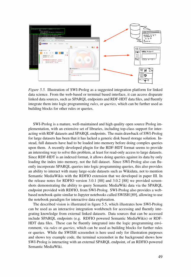
Figure 5.5. Illustration of SWI-Prolog as a suggested integration platform for linkeddata science. From the web-based or terminal based interface, it can access disparatelinked data sources, such as SPARQL endpoints and RDF-HDT data files, and fluentlyintegrate them into logic programming rules, or queries, which can be further used asbuilding blocks for other rules or queries.

SWI-Prolog is a mature, well-maintained and high quality open source Prolog im-plementation, with an extensive set of libraries, including top-class support for inter-acting with RDF datasets and SPARQL endpoints. The main drawback of SWI-Prologfor large datasets has been that it has lacked a generic disk based storage solution. In-stead, full datasets have had to be loaded into memory before doing complex queriesupon them. A recently developed plugin for the RDF-HDT format seems to providean interesting way to solve this problem, at least for read-only access to large datasets.Since RDF-HDT is an indexed format, it allows doing queries against its data by onlyloading the index into memory, not the full dataset. Since SWI-Prolog also can flu-ently incorporate SPARQL queries into logic programming queries, this also providesan ability to interact with many large-scale datasets such as Wikidata, not to mentionSemantic MediaWikis with the RDFIO extension that we developed in paper III. Inthe release notes for RDFIO version 3.0.1 [88] and 3.0.2 [88] we provided screen-shots demonstrating the ability to query Semantic MediaWiki data via the SPARQLendpoint provided with RDFIO, from SWI-Prolog. SWI-Prolog also provides a web-based notebook quite similar to Jupyter notebooks called SWISH [89], allowing to usethe notebook paradigm for interactive data exploration.

The described vision is illustrated in figure 5.5, which illustrates how SWI-Prologcan be used as an interactive integration workbench for accessing and fluently inte-grating knowledge from external linked datasets. Data sources that can be accessedinclude SPARQL endpoints (e.g. RDFIO powered Semantic MediaWikis) or RDF-HDT data files. These can be fluently integrated into the logic programming envi-ronment, via rules or queries, which can be used as building blocks for further rulesor queries. While the SWISH screenshot is here used only for illustration purposesand shows toy example code, the terminal screenshot in the background shows howSWI-Prolog is interacting with an external SPARQL endpoint, of an RDFIO-poweredSemantic MediaWiki.

49

5.6.2 Interactive data analysis and scientific workflowsWe have previously touched upon what can sometimes be experienced as a dualitybetween static, fixed pre-processing pipelines implemented with workflow engines,and the more interactive and exploratory data analysis that is often performed at theend of such data pipelines with the refined datasets coming out of the pre-processingpart.

Firstly, I think there are drawbacks with separating these two modes of data pro-cessing. In our experience from the work in this thesis, one often wants to explorevariations in the data analysis happening also in the pre-processing workflow, whichis with today’s tools often not easily done in an interactive way. Instead, it oftenrequires expert knowledge in workflow development even to make small changes.

At the same time, it is our experience that workflow tools are still far ahead of mostinteractive data exploration environments when it comes to reliably and reproduciblyexecuting large scale analyses, and capturing provenance information about them.

It would thus be interesting to explore what can be done towards providing a high-level interface to data analysis, that fits an interactive, exploratory mode well but thatwould generate workflows in a more traditional workflow tool underneath, when thatis needed.

One of the key goals would be to provide the same interface to querying existingdata as to querying data that does not exist in explicit form, but that could be computedby workflows known to the system. One would describe in a semantic and machinereadable way the capabilities of such workflows, such that the interactive data analysisenvironment can automatically infer when queries can be answered by parametrisingand running such a workflow. Such integrated workflows could thus be said to repre-sent implicit knowledge that can be computed on-demand, quite similar to how rulesin Prolog can be used to infer facts that are not explicitly encoded in raw data but area combination of the plain facts and the rules of the knowledge base.

Here again, it seems SWI-Prolog could be a good foundational platform for imple-menting this because of the flexibility and power of the Prolog language to encapsulatearbitrary logic, and even executions of external programs into rules that generate factson-demand.

Somewhat related research has very recently been published by Gil et. al in [90].Compared to this (excellent) work, the vision presented here would use an approachwith a larger focus on simplicity in terms of technical implementation, to avoid tech-nical debt, and maximising understandability of the full technological stack, as wellas hopefully making the system maintainable by individual researchers.

50

6. Conclusions

In the work in this thesis, we have developed and applied tools and approaches formanaging data and computations in drug discovery in more reproducible and under-standable – thus verifiable – ways.

In specific terms, the conclusions from the studies have been:• The LIBLINEAR method was found to be well suited for large datasets in

ligand-based predictive modelling, where SVM RBF would take too much timeand resources to run. SVM RBF could be preferable for cases when there is alimit to the data available, such that the training time would be limited by thetraining data size anyway (Paper I).

• We found that by using the Flow-based programming principles of separatedependency graph definition and named ports bound to processes, we couldmake development of complex workflows in the Luigi workflow system moreagile and flexible (Paper II).

• We developed a solution for working collaboratively with Semantic Web datasetsin a familiar and user-friendly MediaWiki environment, which allows a reliable,versioned data storage with a powerful templating mechanism for generatingcustom presentations of data and data aggregates. Through the RDFIO exten-sion for Semantic MediaWiki, linked datasets in RDF format can be importedinto and exported out of the wiki environment with retained vocabulary struc-ture (Paper III).

• We developed a solution for publishing large cheminformatics datasets on theweb in the form of a URI resolver that looks up and returns RDF triples relatedto a URI that is being resolved (Paper IV).

• We developed an open source reproducible workflow for building predictivemodels of adverse effects for drug discovery, based on target binding profilestrained on data in a publicly available dataset on drug-target binding. The pre-dictions are implemented with the conformal prediction methodology, whichaddresses the problem of knowing how reliable a certain prediction is, by let-ting the user select a desired confidence level and get predictions – or the lackof predictions – based on that, with guarantees of validity (Paper V).

• We found that by using even more of the principles in Flow-based program-ming, this time including independently and asynchronously running processesconnected with buffered channels, implemented with the CSP-based concur-rency primitives in the Go programming language, we could achieve a verysimple, robust and flexible workflow engine, that has allowed reliably executingthe large scale computations in paper V. It has also allowed rapid developmentof state-of-the-art functionality such as a data-centric provenance feature, andworkflow graph plotting. By focusing on simplicity and re-use of stable, proventechnology, SciPipe also promises to be maintainable in the future by a singleperson or a small team, addressing the problem of sustainability in researchsoftware development (Paper VI).

51

Throughout the work we have came to learn a number of lessons, including thevalue of understandability of computational research. The most important motivationfor this is to make research verifiable, which is also the main motivation behind repro-ducibility. Understandability has additional benefits though, in that it enables to moreeffectively communicate insights and knowledge via the research code, such that itcan be re-used both directly, and indirectly by other researchers and the public.

We have learned that important aspects for maintainability of research softwareand data include simplicity and orthogonality of code and tools, as well as machine-readable data. Automating mundane, repetitive tasks and using tools and frameworkswhich automatically capture provenance information for exploratory analyses, havealso been identified as important parts in making computer-aided research more re-producible and reliable.

52

7. Sammanfattning på Svenska

7.1 Läkemedelsutveckling - en kostsam historiaAtt utveckla nya läkemedel är en lång och kostsam process. Det kan ta så länge somtio till femton år för ett nytt läkemedelsprojekt att nå från idestadium till att komma utpå marknaden. Dessutom misslyckas majoriteten av nya läkemedelskandidater undernågon del av utvecklingprocessen, framförallt i de delar där läkemedlens säkerhet skatestas. En studie uppskattade att endast cirka en av tio läkemedel som når fram till denså kallade kliniska testningsfasen, där läkemedel börjar testas på människor, når framtill ett godkännande av FDA, den Amerikanska motsvarigheten till Läkemedelsverket,för att bli godkända på den Amerikanska marknaden. Oftast är det problem med oön-skade bieffekter som gör att så många läkemedelsprojekt som först verkat så lovande,får skrotas. Problemen med att få ut nya läkemedel på marknaden har dessutom baraväxt för varje år som gått och man talar idag om att läkemedelsindustrin går igenomen produktivitetskris.

Det är tydligt att ju tidigare vi kan förutse vilka läkemedel som kommer att miss-lyckas på grund av oönskade sidoeffekter, desto tidigare kan vi avgöra vilka kemiskasubstanser som är värda att gå vidare med, och vilka som är bättre att lämna i byrålå-dan tillsvidare. Ett av målen med arbetet i den här avhandlingen har varit att ta fram,samt förbättra metoder för att förutse så tidigt som möjligt, vilka läkemedelssubstansersom kan ha problem med oönskade sidoeffekter.

7.2 Problem med återupprepbarhet av analyserSamtidigt med den beskrivna produktivitetskrisen inom läkemedelsbranchen, sker enannan utveckling inom biovetenskaperna. Nya storskaliga automatiserade experi-mentella metoder gör att vi nu kan producera enorma mängder biologiska data, så-som sekvenseringar av DNA och RNA-sekvenser, protein-sekvenser, samt informa-tion från så kallade High-Throughput Screening av kemiska substanser i olika typerav storskaliga, automatiserade tester, för att försöka hitta substanser som uppvisarvissa egenskaper. Kostnaden för att producera sådan storskalig data sjunker dessu-tom stadigt, och man talar idag om att vi redan nått, eller är väldigt nära en omtaladkostnadsgräns på omkring 1000 Amerikanska dollar (ca 10000 kronor) för att göra enkomplett DNA-sekvensering av en människa. Med andra ord så drunknar vi närmasti biologiska data. Aldrig förut har vi kunnat producera så stora datamängder till en såliten kostnad.

Hur har vi kommit till denna till synes paradoxala situation, där vi drunknar i biolo-giska data samtidigt som vi lyckas få ut allt färre nya läkemedel på marknaden? En delforskare tror att det kan ha en koppling till en annan kris som börjat visa sig inom den

53

Figur 7.1. En suggestiv illustration överhur omflyttning och kopiering av data it.ex. Excelfiler, lätt kan leda till att viktigkontextbaserad information om datats in-nebörd går förlorad.

biomedicinska vetenskapen på senare år: En, som man kallar det, reproducerbarhet-skris. Studier som försökt sig på att reproducera (återupprepa) tidigare publiceradestudier inom biomedicin, har misslyckats med att göra detta i en skrämmande stor delav fallen. En del går så långt att påstå att majoriteten av studier inom vissa områ-den inte går att reproducera, och därmed potentiellt påvisar effekter som inte finns iverkligheten, utan snarast beror på slumpmässigheter, eller brus, i datat. Konsensusär också rätt stor inom vetenskapen om att det finns stora problem med reproducer-barhet, vilket bland annat visades i en enkätundersökning bland 1500 forskare, där enmajoritet ansåg att det råder en kris.

Det har förts fram en rad förslag på orsaker till den bristande återupprepbarheten.Till de vanligaste föreslagna orsakerna hör i huvudsak två olika spår. Dels brister i denstatistiska beräkningen av huruvida det man hittat bara beror på slump, eller är teckenpå ett riktigt samband, och dels brister i rapporteringen av alla de steg man tagit föratt genomföra sina experiment.

Det första problemet kan beskrivas enligt följande. Om man till exempel utförexperiment efter experiment i jakten på en indikation på samband mellan några sakerman studerar, tills man hittar en sådan antydan, utan att kompensera för alla de försökman gjort, i sina sannolikhetsberäkningar, så fungerar inte de statistiska metodernasom det är tänkt. Det finns nämligen alltid en viss sannolikhet att få indikationer påsamband av ren slump. De statistiska metoderna behöver därför ta hänsyn till alla deförsök man gjort för att göra en korrekt uppskattning av troligheten att det man hittatär ett verkligt samband, och inte bara slump.

Det andra huvudspåret, att man helt enkelt inte rapporterat de steg man tagit föratt genomföra sitt experiment i tillräcklig detalj för att kunna återupprepa dem, är detsom detta arbete huvudsakligen fokuserar på.

Detta arbete fokuserar också framförallt på datorstödd forskning. Det vill sägaforskning som görs med hjälp av uträkningar och analyser på datorn, baserat på datasom redan tagits fram genom experiment tidigare, till exempel genom de storskaligaexperimentmetoder vi nämnde tidigare.

7.3 Återupprepbarhet och tydlighet inom datorstöddanalys

Inom datorstödd forskning ser frågan om återupprepbarhet en aning annorlunda ut änför experimentell vetenskap där man gör experiment i den fysiska världen. En dator är

54

ett väldigt exakt instrument, och det händer i princip aldrig att den räknar fel, såvidaman inte programmerat den fel.

Men för det första så kan man faktiskt få problem med återupprepbarhet ändå,till exempel om man bara klickat manuellt i ett grafiskt program, och inte har doku-menterat tillräckligt väl hur man gjort denna manuella del av analysen. Generellt kanman därför säga att det är bra att försöka utforma sin analys i form av ett körbartscript eller program istället, för att undvika dessa problem, eftersom alla detaljer dåav nödvändighet blir dokumenterade i form av programkod.

Det finns dock andra problem med analyser som görs på datorer, även om de skullevara aldrig så väl kodade i skript eller program. Ett viktigt sådant är att det är lätt atttappa kollen på vad ens datorprogram egentligen gör. På datorn har man sällan sammadirekta kontakt med sina instrument och undersökningsmaterial som man har i denfysiska världen. Man kan inte på samma sätt se, höra, röra eller känna lukten av detsom försiggår när det bara sker virtuellt, inuti en dator. Det är tyvärr rätt vanligt attforskare som använder analysprogram på datorn, använder dem som en sorts "svartlåda", där man lägger in värden i ena änden, och får ut värden i den andra, men sällaröppnar lådan för att försöka förstå hur den fungerar inuti. Det här är ett stort problemeftersom det mycket väl kan hända att någon ibland har programmerat fel. Det ärdessutom viktigt att verkligen förstå alla antaganden som ett visst datorprogram gör.Det är nämligen inte säkert att den som skapat programmet alltid har dokumenterat såväl exakt alla antaganden och förutsättningar som programmet gör, utan det är viktigtatt andra forskare kan skapa sig en bild av detta själva.

7.4 Problem med tydlighet i innebörden avforskningsdata

Om vi går vidare så finns det fler områden där datorstödd forskning kan stöta på prob-lem. Om vi nyss talade om svårigheten att få grepp om vad datorprogram egentligengör, så ska vi nu säga något om problemet med att veta vad lagrade data verkligenbetyder. Just detta, att ha koll på vad en fil med data betyder, är nämligen långt ifrånså enkelt som det låter. Tänk dig till exempel en Excelfil. Hur kan man där veta vadvärdena i olika celler i ett kalkylblad betyder? Om man har tur så har något beskrivitutförligt i anslutning till varje cell, eller åtminstone kolumn eller rad, vad varje sådanbetyder, men det är inget vi kan ta för givet. Dessutom kan språkliga beskrivningarlätt bli ganska otydliga. En person kan lätt missuppfatta vad en annan menade. Dessu-tom finns det problem som uppstår då man kopierar eller flyttar data mellan olikakalkylblad och arbetsböcker i t.ex. Excel. Då kan det lätt hända att man mistar ävenden information som faktiskt fanns om datat. Man kan säga att man lätt kan tappakontextberoende information, när datat flyttas ur sin ursprungliga kontext. Figur 7.1försöker att illustrera detta på ett lite suggestivt sätt. Det här är ett ganska stort prob-lem med forskningsdata som sparas i enkla textformat eller kalkylblad, nämligen attman inte har någon exakt, otvetydig definition av vad data betyder. Det gör det lätthänt att någon använder data på ett sätt som dataskaparen inte alls tänkt sig.

För att ge några konkreta exempel så skulle det kunna röra sig om att man hardata om en organism, t.ex. mus, som man av misstag tror hör till en annan organism,t.ex. människa, eller att man utgår ifrån fel enhet på uppmätta värden, t.ex. mikroliter

55

istället för milliliter (ett fel på 1000 gånger!). Sådana till synes enkla fel kan ledatill digra konsekvenser när annan forskning börjar bygga på forskningsdata som blivitfelaktigt tolkad.

7.5 Lösningar på problemenEn del av målsättningarna med den här avhandlingen har varit att adressera de härproblemen. Det vill säga, dels hur vi kan göra datoranalyser mer automatiserade,samtidigt som de blir någorlunda lätta att överblicka och förstå. Dels med att göradet lättare att hantera data på ett smart sätt, där viktig så kallad metadata (d.v.s. dataom datat) kan sparas tillsammans med data. Sådan metadata kan nämligen användasför att beskriva på ett mer exakt sätt vad data betyder, och i bästa fall till och medinnehålla en full beskrivning av exakt hur datat skapades, så att den som använder datatverkligen kan bedöma dess giltighet, och I bästa fall till och med kan använda dennainformation för att själv räkna fram en ny version av datat, kanske med lite justeradeparametrar, eller med ny information som inte fanns tillgänglig när det ursprungligadatat togs fram. Nedan följer en lite mer ingående beskrivning av hur vi adresseratdessa problem.

7.5.1 Bättre upprepbarhet och tydlighet i datoranalyser medförbättrade arbetsflödesverktyg

Vi har utvecklat två olika lösningar för att automatisera datorstödd analys på ett sättsom gör att man inte behöver peka och klicka i ett grafiskt program, utan lägger inhela sin analys i ett körbart script, som vem som helst, när som helst kan köra om föratt verifiera resultaten. Detta har gjorts genom att utveckla två datorprogram av entyp som kallas arbetsflödesverktyg. Arbetsflödesverktyg fungerar så att man beskriversin analys på en nivå där det är någorlunda lätt att se helheten i sin analys, medanman låter arbetsflödesverktyget ta hand om lågnivå-detaljer såsom att se till att filersparas med rätt filnamn och att programmet går att starta om ifall det kraschade utanatt läsa in halvfärdiga, trasiga data. Ett av arbetsflödesverktygen vi utvecklat heterSciLuigi, och baseras på ett system som heter Luigi, som är utvecklat av Spotify föratt räkna ut topplistor för låtar i Spotify-appen. Det andra verktyget, som vi kallarSciPipe, är skrivet helt från grunden i Googles nya programmeringsspråk Go. SciPipebygger vidare på lärdomar från byggandet av SciLuigi, men gör det med en förbättradoch enklare grund, som gör att systemet är optimerat för tydlighet, enkelhet, flexibilitetoch prestanda från första början. Aspekter som vi upptäckt vara viktiga vid storskaligadataanalyser inom vårt forskningsområde.

Gemensamt för båda dessa system är att de dragit nytta av principer från ett tänkesättför programmering som kallas flödesbaserad programmering (Flow-based program-ming på Engelska). Flödesbaserad programmering bygger på en princip som närmastkan liknas vid en fabrik byggd på löpande-band principen, där det finns massor avstationer där arbete utförs, och där sedan arbetsmaterialet, t.ex. bilar, färdas på rull-band eller skenor mellan stationerna. Dessa stationer jobbar då både självständigt ochparallellt, med en hög total prestanda som resultat, och de synkroniserar med varan-dra enbart via det arbetsmaterial som färdas på löpbanden, vilket är en enkel, flexibel

56

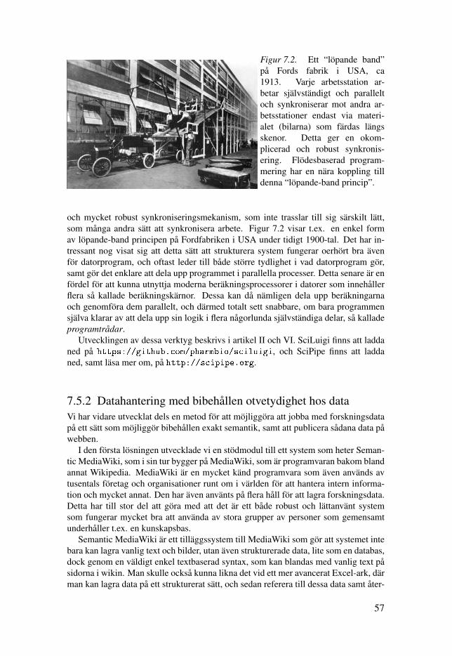
Figur 7.2. Ett “löpande band”på Fords fabrik i USA, ca1913. Varje arbetsstation ar-betar självständigt och paralleltoch synkroniserar mot andra ar-betsstationer endast via materi-alet (bilarna) som färdas längsskenor. Detta ger en okom-plicerad och robust synkronis-ering. Flödesbaserad program-mering har en nära koppling tilldenna “löpande-band princip”.

och mycket robust synkroniseringsmekanism, som inte trasslar till sig särskilt lätt,som många andra sätt att synkronisera arbete. Figur 7.2 visar t.ex. en enkel formav löpande-band principen på Fordfabriken i USA under tidigt 1900-tal. Det har in-tressant nog visat sig att detta sätt att strukturera system fungerar oerhört bra ävenför datorprogram, och oftast leder till både större tydlighet i vad datorprogram gör,samt gör det enklare att dela upp programmet i parallella processer. Detta senare är enfördel för att kunna utnyttja moderna beräkningsprocessorer i datorer som innehållerflera så kallade beräkningskärnor. Dessa kan då nämligen dela upp beräkningarnaoch genomföra dem parallelt, och därmed totalt sett snabbare, om bara programmensjälva klarar av att dela upp sin logik i flera någorlunda självständiga delar, så kalladeprogramtrådar.

Utvecklingen av dessa verktyg beskrivs i artikel II och VI. SciLuigi finns att laddaned på https://github.com/pharmbio/sciluigi, och SciPipe finns att laddaned, samt läsa mer om, på http://scipipe.org.

7.5.2 Datahantering med bibehållen otvetydighet hos dataVi har vidare utvecklat dels en metod för att möjliggöra att jobba med forskningsdatapå ett sätt som möjliggör bibehållen exakt semantik, samt att publicera sådana data påwebben.

I den första lösningen utvecklade vi en stödmodul till ett system som heter Seman-tic MediaWiki, som i sin tur bygger på MediaWiki, som är programvaran bakom blandannat Wikipedia. MediaWiki är en mycket känd programvara som även används avtusentals företag och organisationer runt om i världen för att hantera intern informa-tion och mycket annat. Den har även använts på flera håll för att lagra forskningsdata.Detta har till stor del att göra med att det är ett både robust och lättanvänt systemsom fungerar mycket bra att använda av stora grupper av personer som gemensamtunderhåller t.ex. en kunskapsbas.

Semantic MediaWiki är ett tilläggssystem till MediaWiki som gör att systemet intebara kan lagra vanlig text och bilder, utan även strukturerade data, lite som en databas,dock genom en väldigt enkel textbaserad syntax, som kan blandas med vanlig text påsidorna i wikin. Man skulle också kunna likna det vid ett mer avancerat Excel-ark, därman kan lagra data på ett strukturerat sätt, och sedan referera till dessa data samt åter-

57

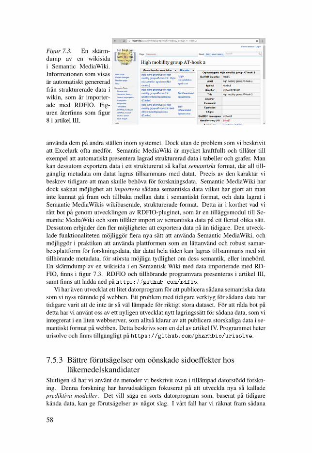
Figur 7.3. En skärm-dump av en wikisidai Semantic MediaWiki.Informationen som visasär automatiskt genereradfrån strukturerade data iwikin, som är importer-ade med RDFIO. Fig-uren återfinns som figur8 i artikel III,

använda dem på andra ställen inom systemet. Dock utan de problem som vi beskrivitatt Excelark ofta medför. Semantic MediaWiki är mycket kraftfullt och tillåter tillexempel att automatiskt presentera lagrad strukturerad data i tabeller och grafer. Mankan dessutom exportera data i ett strukturerat så kallat semantiskt format, där all till-gänglig metadata om datat lagras tillsammans med datat. Precis av den karaktär vibeskrev tidigare att man skulle behöva för forskningsdata. Semantic MediaWiki hardock saknat möjlighet att importera sådana semantiska data vilket har gjort att maninte kunnat gå fram och tillbaka mellan data i semantiskt format, och data lagrat iSemantic MediaWikis wikibaserade, strukturerade format. Detta är i korthet vad virått bot på genom utvecklingen av RDFIO-pluginet, som är en tilläggsmodul till Se-mantic MediaWiki och som tillåter import av semantiska data på ett flertal olika sätt.Dessutom erbjuder den fler möjligheter att exportera data på än tidigare. Den utveck-lade funktionaliteten möjliggör flera nya sätt att använda Semantic MediaWiki, ochmöjliggör i praktiken att använda plattformen som en lättanvänd och robust samar-betsplattform för forskningsdata, där datat hela tiden kan lagras tillsammans med sintillhörande metadata, för största möjliga tydlighet om dess semantik, eller innebörd.En skärmdump av en wikisida i en Semantisk Wiki med data importerade med RD-FIO, finns i figur 7.3. RDFIO och tillhörande programvara presenteras i artikel III,samt finns att ladda ned på https://github.com/rdfio.

Vi har även utvecklat ett litet datorprogram för att publicera sådana semantiska datasom vi nyss nämnde på webben. Ett problem med tidigare verktyg för sådana data hartidigare varit att de inte är så väl lämpade för riktigt stora dataset. För att råda bot pådetta har vi använt oss av ett nyligen utvecklat nytt lagringssätt för sådana data, som viintegrerat i en liten webbserver, som alltså klarar av att publicera storskaliga data i se-mantiskt format på webben. Detta beskrivs som en del av artikel IV. Programmet heterurisolve och finns tillgängligt på https://github.com/pharmbio/urisolve.

7.5.3 Bättre förutsägelser om oönskade sidoeffekter hosläkemedelskandidater

Slutligen så har vi använt de metoder vi beskrivit ovan i tillämpad datorstödd forskn-ing. Denna forskning har huvudsakligen fokuserat på att utveckla nya så kalladeprediktiva modeller. Det vill säga en sorts datorprogram som, baserat på tidigarekända data, kan ge förutsägelser av något slag. I vårt fall har vi räknat fram sådana

58

prediktiva modeller på data om problematiska sidoeffekter hos potentiella läkemedelssub-stanser. Med andra ord så har modellerna blivit tränade att kunna förutsäga huruvidaen viss kemisk substans har sådana problem eller ej. Vi har gjort detta arbete i tvåsteg. I artikel I, som är av något mer teknisk karaktär, så undersöker vi först hur välden prediktiva (förutsägande) förmågan påverkas av storleken på de data man använ-der för att bygga upp, eller träna, modellerna. Vi ställer denna förmåga mot den tid dettar att träna modellerna, eftersom det är viktigt att denna träning kan avslutas i rimligtid. En datorkörning som tar längre än sju dagar, är till exempel sällan praktisk, dårisken att något ska gå snett under träningen då ökar drastiskt. I artikel I hittade vi enbra avvägning mellan datasetstorlek och prediktiv förmåga, samt upptäckte att en avde två metoder vi utvärderat var mer lämpat än den andra för riktigt stora dataset. Idenna artikel använde vi arbetsflödesverktyget som presenteras i artikel II.

I artikel V går vi in på vår sluttillämpning, nämligen att bygga modeller somförutsäger oönskade sidoeffekter hos kemiska substanser. Sättet som vi byggt dessamodeller är att basera dem på data om bindning mellan kemiska molekyler och mål-molekyler i kroppen (i princip alltid proteiner). Genom att då plocka ut data om ettantal (31 st) kända problematiska målproteiner som läkemedel helst inte alls ska bindatill, samt data om de molekyler som man vet redan binder till dessa, så fick vi fram31 stycken modeller, en för varje målmolekyl i kroppen. Var och en av dessa kansedan, givet en frågemolekyl, säga något om risken för bindning till respektive mål-protein för denna frågemolekyl. Vi har sedan lagt ihop dessa 31 modeller till en såkallad bindningprofil, och gjort bland annat en webbsida där man kan lägga in kemiskmolekyl man vill veta mer om och få tillbaka ett svar med en förutsägelse om huru-vida “frågemolekylen” ser ut som att den skulle binda till någon av de problematiskamålproteinerna eller ej. Vi använder dessutom ett nytt sätt att göra sådana prediktionerpå, som ger mer information om pålitligheten i de förutsägelse man får, där man självkan ställa in på ett reglage från noll till ett, hur stor så kallad konfidens man vill ha isina förutsägelser. Detta fungerar då som ett slags filter och gör att man enbart ser deresultat som når över den konfidensnivå man väljer. Webbsidan finns tillgänglig atttesta på http://modelingweb.service.pharmb.io/predict/profile/ptp.

7.6 SlutkommentarSammanfattningsvis har vi alltså utvecklat metoder som ämnar att förbättra återup-prepbarhet samt tydlighet i datorstödda dataanalyser, samt att möjliggöra hanteringav data på ett sätt som gör att metadata om datats ursprungliga innebörd kan lagrastillsammans med datat, både för kollaborativt arbete med datat, samt för att publiceradatat på webben. Slutligen så har vi använt några av våra utvecklade metoder för attutveckla nya bättre datorprogram (så kallade prediktiva modeller) som kan förutsägaoönskade sidoeffekter hos potentiella läkemedelssubstanser på ett tidigt stadium.

Förhoppningsvis kan dessa metoder sammantaget i någon mån adressera de prob-lem vi lyfte fram i början av den här sammanfattningen, angående återupprepbarhetoch tydlighet i datorstödd forskning, och därmed kanske även problemen med sjunkandeproduktivitet och skenande kostnader inom utvecklingen av nya läkemedel. Kan degöra det så är denna avhandlings målsättning uppnådd.

59

8. Acknowledgements

This work was carried out in the Pharmaceutical Bioinformatics group at the Depart-ment of Pharmaceutical Biosciences, division of Pharmacology, Faculty of Pharmacy,Uppsala University, Sweden.

I am grateful to many, but would like to thank in particular the following people,who have meant much to me while working on this thesis:

My supervisor Assoc. Prof. Ola Spjuth for letting me do this work in the group,and for incredible tireless encouragement and support. I have learned so much, and ithas meant so much to me, personally and professionally. I do not really know how tothank you properly.

My co-supervisor Prof. Roland Grafström for inspiring collaboration work andgreat advice of a type that is found only with the most experienced.

Head of department, Prof. Björn Hellman for always greeting even us PhD stu-dents cordially every day. You are a great example for us all.

Prof. Jarl Wikberg, for encouragement and welcoming during my masters stud-ies, when I first came in contact with the group.

My colleagues, past and present, at Farmbio. In particular Jonathan Alvarsson,who I have had the pleasure to work with over a number of projects and learned somuch from. I have deeply appreciated your honesty and caring advice, as from anolder brother-in-research. Arvid Berg, always ready to support with technical issues,great orienteering advice and good company. Staffan Arvidsson Mc Shane for pa-tiently answering my bugging you about conformal prediction. Wesley Schaal forhelping out with crucial scientific advice and language proofing many times. Mar-tin Dahlö, for a very valuable contribution in making SciPipe useful for sequencingbioinformatics. Marco Capuccini and Jon Ander Novella for great and insightfulcloud-computing discussions. Jonathan, Arvid, Maris, Marco, Jon, Staffan, Wes,Martin, Valentin, Polina, Aleh, Sviatlana, Phil, Anders, Matteo, Niharika, Juan,Alexander, and Tanya, as well as affiliated colleagues Stephanie, Payam, Kim andLaeeq, for great times all around. I have deeply enjoyed getting to know you, and towork with some of you. You’re such a great bunch, making up a great team. Keep upthe positive spirit.

All the administrative folks at Farmbio, particularly Marina Rönngren, for alwaysfiguring out our paper-work mess, always with a smile and kind word.

60

All my NBIS/SciLifeLab colleagues. In particular my bosses Prof. Bengt Persson,Mikael Borg and Jonas Hagberg for allowing me to combine my part-time PhD withwork at NBIS for some time, as well as kind encouragement and good time workingtogether. Johan Dahlberg, for highly valuable feedback and encouragement from afellow workflow expert. Johan Hermansson for encouragement and inspiring chats.Roman Valls Guimerà and Per Kraulis for interesting discussions. All at Gamma 6,in particular Linus Östberg, Jorrit Boekel, Ino De Bruijn, Niclas Jareborg, IkramUllah and others, and everyone on the SciLifeLab slack, for good chats and cheers.

My half-time reviewers Assoc. Prof. Andreas Hellander, Salman Toor andMikael Huss for helpful feedback and encouragement.

Egon Willighagen for continuing to be something of a mentor long after I’m nolonger formally your student. I have so many things to thank you for. Learning thevalue of open science, or even something seemingly – but not truly – trivial as blog-ging and tweeting in research, are all but parts of that.

My collaborators. Pekka Kohonen, Ines Smit, Ali King, Maciej Kanduła andDavid Kreil for interesting collaborations. Matthias Palmér and Fernanda Dóreafor a great time co-organising the Linked Data Sweden event, and Johan Rung,Hanna Kultima, and Erika Bergqvist Erkstam for valuable support from SciL-ifeLab’s side. Chanin Nantasenamat, Björn Grüning, Dan Blankenberg, AdamAmeur, Björn Nystedt and others, for interesting co-authorship projects.

Denny Vrandecic for mentoring me during my Google summer of code project,for kindly sharing ideas and encouragement which helped ignite the RDFIO project.Joel Sachs for co-mentoring Ali King for the Gnome FOSS OPW program for RD-FIO. James Hongkong, Karsten Hoffmeyer and Jeroen De Dauw for support andencouragement with the RDFIO project.

Many people I had great exchange with over the internet. In particular John PaulMorrison, for generously sharing ideas and time for discussion in the FBP discus-sion group, Vladimir Sibirov for generously sharing the GoFlow library from which Ilearned much, Egon Elbre for important feedback that improved SciPipe a lot, DanielWhitenack for encouragement and fun collaboration in the GopherData communityand Jörgen Brandt, Simone Bafelli, Paolo Di Tommaso, Michael R. Crusoe, PeterAmstutz, John Chilton, Pierre Lindenbaum, Jeff Gentry and others with whomI have benefited from many very useful discussions on workflows, science and pro-gramming.

61

My friends Lauri, Jan, Yonas, David K, Kaleb, Simon C, Mattias H, Boby andIurii for your loyal friendship over the years. It has meant a lot. Thank you pastorEdward, and the whole gang at Cross Culture church, in particular James, Moses,Simon, Jonas and Linh, Timmy, Annie and others. Thank you also, Petter andConcessa, for kind friendship and support during our time in Uppsala.

My family. My father Rolf, for countless hours of feedback, brainstorming, adviceand overall support and encouragement. A few words on a page can not make justiceto the value of this, for this thesis and otherwise. My mother Mariann, "Anne", forhelping out in so many ways over the years. If everybody were as willing to lovinglycare and help as you, the world would not have many problems left. My brothers andsisters, Sandra, Simon, Theresa, Jonathan, Elias and Miryam, for always beingsuch a loving and supporting family. My cousins Micke and Mackan, who are likebrothers, ready to help whenever there is a need.

The support from my (large) extended family has also been valuable.First, a big kudos to Jan Lampa, for letting me use the photo on the cover, which

he took at the Storforsen rapid in Norrbotten county in Northern Sweden, where alsothe respondent was born and raised.

A special thanks also to godparent Lis-Marie who has always been very support-ive, Åsa and Peyman for receiving us so cordially on our trip to Luleå, my uncle withwife Håkan and Ann-Christin, for generosity and support when visiting Gävle, auntLena and Gustav, for receiving us for a good time in Jakobstad, and my grandparentsPer and Gerda for for kind support.

A special thanks to my dear wife Emebet, for so faithfully and lovingly standingby my side through these intensive and stressful years. I owe you so much. Thank you!

My family on my wife’s side has also been supportive in important ways duringthese intensive years. I’m thankful to all of you, but a special thanks to Kassa for al-ways encouraging my studies, Berhanu and Zewditu with family for very generoushosting of us during our much needed vacations in Addis Abeba in the middle of theSwedish winter (but Ethiopian sunny dry-season), and Azeb and Tekle, Misrak withfamily and Hanna with family, and Meseret, for love and care, and all you young-sters too.

A special thanks also to Dereje, Eshetu and Elsa, for kindly supporting and help-ing us during our last stay in Addis, and Prof. Abebe Getahun for receiving us for avery interesting visit to Addis Ababa University. Hope to manage to get some collab-orations going eventually.

Last but not least my Lord and Saviour, who is my wisdom and strength, andthrough whom all I do is made possible. In your light I see light.

62

References

[1] Fabio Pammolli, Laura Magazzini, and Massimo Riccaboni. The productivitycrisis in pharmaceutical R&D. Nature reviews Drug discovery, 10(6):428, 2011.

[2] Vivien Marx. Biology: The big challenges of big data. Nature,498(7453):255–260, 2013.

[3] Zachary D. Stephens, Skylar Y. Lee, Faraz Faghri, Roy H. Campbell,Chengxiang Zhai, Miles J. Efron, Ravishankar Iyer, Michael C. Schatz, SaurabhSinha, and Gene E. Robinson. Big data: Astronomical or genomical? PLoSBiology, 13(7):1–11, 2015.

[4] Stephen V Frye, Michelle R Arkin, Cheryl H Arrowsmith, P Jeffrey Conn,Marcie A Glicksman, Emily A Hull-Ryde, and Barbara S Slusher. Tacklingreproducibility in academic preclinical drug discovery. Nature Reviews DrugDiscovery, 14(11):733, 2015.

[5] Jack W. Scannell and Jim Bosley. When Quality Beats Quantity: DecisionTheory, Drug Discovery, and the Reproducibility Crisis. PLOS ONE,11(2):1–21, 02 2016.

[6] Monya Baker. 1,500 scientists lift the lid on reproducibility. Nature News,533(7604):452, 2016.

[7] Marcus R Munafò, Brian A Nosek, Dorothy VM Bishop, Katherine S Button,Christopher D Chambers, Nathalie Percie du Sert, Uri Simonsohn, Eric-JanWagenmakers, Jennifer J Ware, and John PA Ioannidis. A manifesto forreproducible science. Nature Human Behaviour, 1(1):0021, 2017.

[8] Konrad Hinsen. Verifiability in computer-aided research: the role of digitalscientific notations at the human-computer interface. PeerJ Computer Science,4:e158, 2018.

[9] Graham L Patrick. An introduction to medicinal chemistry. Oxford universitypress, 6 edition, 2017.

[10] Rita Santos, Oleg Ursu, Anna Gaulton, A Patrícia Bento, Ramesh S Donadi,Cristian G Bologa, Anneli Karlsson, Bissan Al-lazikani, Anne Hersey, Tudor IOprea, and John P Overington. A comprehensive map of molecular drugtargets. Nature Publishing Group, 16(1):19–34, 2016.

[11] Muhammed A. Yildirim, Kwang Il Goh, Michael E. Cusick, Albert LászlóBarabási, and Marc Vidal. Drug-target network. Nature Biotechnology,25(10):1119–1126, 2007.

[12] Douglas B. Kitchen, Hélène Decornez, John R. Furr, and Jürgen Bajorath.Docking and scoring in virtual screening for drug discovery: Methods andapplications. Nature Reviews Drug Discovery, 3(11):935–949, 2004.

[13] Paul L Herrling. The drug discovery process. Progress in drug research,62:1–14, 2005.

[14] Michael Hay, David W Thomas, John L Craighead, Celia Economides, andJesse Rosenthal. Clinical development success rates for investigational drugs.Nat Biotech, 32(1):40–51, 2014.

63

[15] Joseph A DiMasi, Henry G Grabowski, and Ronald W Hansen. Innovation inthe pharmaceutical industry: new estimates of R&D costs. Journal of healtheconomics, 47:20–33, 2016.

[16] A Bartlett, B Penders, and J Lewis. Bioinformatics: indispensable, yet hidden inplain sight? BMC Bioinformatics, 18(1):311, 2017.

[17] Francis Crick. Central dogma of molecular biology. Nature, 227(5258):561,1970.

[18] David S Wishart. Bioinformatics for Metabolomics. Genomics, pages 581–599,2009.

[19] Egon L Willighagen, Nina Jeliazkova, Barry Hardy, Roland C Grafström, andOla Spjuth. Computational toxicology using the OpenTox applicationprogramming interface and Bioclipse. BMC Research Notes, 4(1):487, 2011.

[20] David J Wild. Grand challenges for cheminformatics. Journal ofcheminformatics, 1:1, jan 2009.

[21] Artem Cherkasov, Eugene N. Muratov, Denis Fourches, Alexandre Varnek,Igor I. Baskin, Mark Cronin, John Dearden, Paola Gramatica, Yvonne C.Martin, Roberto Todeschini, Viviana Consonni, Victor E. Kuz’min, RichardCramer, Romualdo Benigni, Chihae Yang, James Rathman, Lothar Terfloth,Johann Gasteiger, Ann Richard, and Alexander Tropsha. Qsar modeling: Wherehave you been? where are you going to? Journal of Medicinal Chemistry,57(12):4977–5010, 2014. PMID: 24351051.

[22] E C Ibezim, P R Duchowicz, and N E Ibezim. Computer-Aided LinearModeling Employing Qsar for Drug Discovery. Pharmaceutical Technology,1(1900):76–82, 2009.

[23] Jeff Gauthier, Antony T Vincent, Steve J Charette, and Nicolas Derome. A briefhistory of bioinformatics. Briefings in Bioinformatics, page bby063, 2018.

[24] Margaret O Dayhoff and National Biomedical Research Foundation. Atlas ofprotein sequence and structure, 1, 1965.

[25] Michael L Metzker. Sequencing technologies - the next generation. Nat RevGenet, 11:31–46, Jan 2010.

[26] Robert P Hertzberg and Andrew J Pope. High-throughput screening: newtechnology for the 21st century. Current Opinion in Chemical Biology, 4(4):445– 451, 2000.

[27] A. Lavecchia and C. Di Giovanni. Virtual screening strategies in drugdiscovery: A critical review. Current Medicinal Chemistry, 20(March2016):2839–2860, 2013.

[28] David B Searls. Data integration: challenges for drug discovery. Naturereviews. Drug discovery, 4(1):45–58, 2005.

[29] Ola Spjuth, Erik Bongcam-Rudloff, Guillermo Carrasco Hernández, LukasForer, Mario Giovacchini, Roman Valls Guimera, Aleksi Kallio, EijaKorpelainen, Maciej M Kanduła, Milko Krachunov, et al. Experiences withworkflows for automating data-intensive bioinformatics. Biology direct,10(1):43, 2015.

[30] Alexey Siretskiy, Tore Sundqvist, Mikhail Voznesenskiy, and Ola Spjuth. Aquantitative assessment of the Hadoop framework for analyzing massivelyparallel DNA sequencing data. GigaScience, 4(1):26, 2015.

[31] Ola Spjuth, Erik Bongcam-Rudloff, Johan Dahlberg, Martin Dahlö, Aleksi

64

Kallio, Luca Pireddu, Francesco Vezzi, and Eija Korpelainen.Recommendations on e-infrastructures for next-generation sequencing.GigaScience, 5(1):26, 2016.

[32] Sarah Cohen-boulakia, Khalid Belhajjame, Olivier Collin, Jérôme Chopard,Yvan Le, Frédéric Lemoine, Fabien Mareuil, and Hervé Ménager. Scientificworkflows for computational reproducibility in the life sciences : Status ,challenges and opportunities. Future Generation Computer Systems, pages1–15, 2017.

[33] David Gomez-Cabrero, Imad Abugessaisa, Dieter Maier, Andrew Teschendorff,Matthias Merkenschlager, Andreas Gisel, Esteban Ballestar, ErikBongcam-Rudloff, Ana Conesa, and Jesper Tegnér. Data integration in the eraof omics: current and future challenges. BMC systems biology, 8 Suppl 2(2):I1,2014.

[34] Akram Alyass, Michelle Turcotte, and David Meyre. From big data analysis topersonalized medicine for all: challenges and opportunities. BMC MedicalGenomics, 8(1):33, 2015.

[35] John P A Ioannidis. Why most published research findings are false. PLoSMedicine, 2(8):0696–0701, 2005.

[36] Luxi Shen and Oleg Urminsky. Making sense of replications. pages 1–9, 2017.[37] Konrad Hinsen. Computational science: shifting the focus from tools to models.

F1000Research, 101(May 2014), 2014.[38] Jianwu Wang, Daniel Crawl, Shweta Purawat, Mai Nguyen, and Ilkay Altintas.

Big data provenance: Challenges, state of the art and opportunities. InProceedings - 2015 IEEE International Conference on Big Data, IEEE BigData 2015, 2015.

[39] Ross Ihaka and Robert Gentleman. R: a language for data analysis and graphics.Journal of computational and graphical statistics, 5(3):299–314, 1996.

[40] R Core Team. R: A language and environment for statistical computing.http://www.R-project.org/, 2017.

[41] Ola Spjuth, Tobias Helmus, Egon L Willighagen, Stefan Kuhn, Martin Eklund,Johannes Wagener, Peter Murray-Rust, Christoph Steinbeck, and Jarl ESWikberg. Bioclipse: an open source workbench for chemo-and bioinformatics.BMC bioinformatics, 8(1):59, 2007.

[42] Ola Spjuth, Jonathan Alvarsson, Arvid Berg, Martin Eklund, Stefan Kuhn, CarlMäsak, Gilleain Torrance, Johannes Wagener, Egon L Willighagen, ChristophSteinbeck, et al. Bioclipse 2: A scriptable integration platform for the lifesciences. BMC bioinformatics, 10(1):397, 2009.

[43] Jeremy Leipzig. A review of bioinformatic pipeline frameworks. Briefings inBioinformatics, (January):bbw020, 2016.

[44] Jeremy Leipzig. Computational Pipelines and Workflows in Bioinformatics.Reference Module in Life Sciences, pages 1–11, 2018.

[45] T. Oinn, M. Greenwood, M. Addis, N. Alpdemir, J. Ferris, K. Glover, C. Goble,A. Goderis, D. Hull, D. Marvin, P. Li, P. Lord, M. Pocock, M. Senger,R. Stevens, A. Wipat, and C. Wroe. Taverna: lessons in creating a workflowenvironment for the life sciences. Concurr. Comput., 18, 2006.

[46] Daniel Blankenberg, Gregory Von Kuster, Nathaniel Coraor, GuruprasadAnanda, Ross Lazarus, Mary Mangan, Anton Nekrutenko, and James Taylor.

65

Galaxy: A Web-Based Genome Analysis Tool for Experimentalists. John Wiley& Sons, Inc., Hoboken, 2010.

[47] Belinda Giardine, Cathy Riemer, Ross C. Hardison, Richard Burhans, LauraElnitski, Prachi Shah, Yi Zhang, Daniel Blankenberg, Istvan Albert, JamesTaylor, Webb Miller, W. James Kent, and Anton Nekrutenko. Galaxy: Aplatform for interactive large-scale genome analysis. Genome Res.,15(10):1451–1455, 2005.

[48] B. Giardine, C. Riemer, R. C. Hardison, R. Burhans, L. Elnitski, P. Shah,Y. Zhang, D. Blankenberg, I. Albert, J. Taylor, W. Miller, W. J. Kent, andA. Nekrutenko. Galaxy: a platform for interactive large-scale genome analysis.Genome Res., 15, 2005.

[49] Jeremy Goecks, Anton Nekrutenko, and James Taylor. Galaxy: acomprehensive approach for supporting accessible, reproducible, andtransparent computational research in the life sciences. Genome Biol.,11(8):1–13, 2010.

[50] Adam A. Hunter, Andrew B. Macgregor, Tamas O. Szabo, Crispin A.Wellington, and Matthew I. Bellgard. Yabi: An online research environment forgrid, high performance and cloud computing. Source Code Biol. Med.,7(1):1–10, 2012.

[51] Johannes Köster and Sven Rahmann. Snakemake—a scalable bioinformaticsworkflow engine. Bioinformatics, 28(19):2520–2522, 2012.

[52] Simon P. Sadedin, Bernard Pope, and Alicia Oshlack. Bpipe: a tool for runningand managing bioinformatics pipelines. Bioinformatics, 28(11):1525–1526,2012.

[53] Paolo Di Tommaso, Maria Chatzou, Pablo Prieto Baraja, and CedricNotredame. A novel tool for highly scalable computational pipelines. 12 2014.

[54] Luigi source code on GitHub. https://github.com/spotify/luigi.Accessed 5 April 2016.

[55] Jörgen Brandt, Marc Bux, and Ulf Leser. Cuneiform: a functional language forlarge scale scientific data analysis. In EDBT/ICDT Workshops, pages 7–16,2015.

[56] The FAIR Guiding Principles for scientific data management and stewardship.Scientific Data, 3:160018, 2016.

[57] Tim Berners-Lee, James Hendler, and Ora Lassila. The Semantic Web. Sci.Am., 284(5):34–43, 2001.

[58] Eric Miller, Ralph Swick, and Dan Brickley. Resource description framework(RDF). W3C Recommendation, W3C, 2004.

[59] Andy Seaborne and Eric Prud’hommeaux. SPARQL query language for RDF.W3C recommendation, W3C, January 2008.

[60] Frank van Harmelen and Deborah McGuinness. OWL web ontology languageoverview. W3C recommendation, W3C, February 2004.

[61] World Wide Web Consortium et al. JSON-LD 1.0: a JSON-based serializationfor linked data. W3C recommendation, W3C, 2014.

[62] Mark D. Wilkinson, Ruben Verborgh, Luiz Olavo Bonino da Silva Santos, TimClark, Morris A. Swertz, Fleur D.L. Kelpin, Alasdair J.G. Gray, Erik A.Schultes, Erik M. van Mulligen, Paolo Ciccarese, Arnold Kuzniar, AnandGavai, Mark Thompson, Rajaram Kaliyaperumal, Jerven T. Bolleman, and

66

Michel Dumontier. Interoperability and FAIRness through a novel combinationof Web technologies. PeerJ Computer Science, 3:e110, April 2017.

[63] Philippe Rocca-Serra, Marco Brandizi, Eamonn Maguire, Nataliya Sklyar,Chris Taylor, Kimberly Begley, Dawn Field, Stephen Harris, Winston Hide,Oliver Hofmann, Steffen Neumann, Peter Sterk, Weida Tong, Susanna AssuntaSansone, and Jonathan Wren. ISA software suite: Supportingstandards-compliant experimental annotation and enabling curation at thecommunity level. Bioinformatics, 27(13):2354–2356, 2011.

[64] Stuart J. Chalk. SciData: A data model and ontology for semanticrepresentation of scientific data. Journal of Cheminformatics, 8(1):1–24, 2016.

[65] Jean-loup Faulon. The Signature Molecular Descriptor . 1 . Using ExtendedValence Sequences in QSAR and QSPR Studies. pages 707–720, 2003.

[66] Jonathan Alvarsson. Ligand-based Methods for Data Management andModelling. PhD thesis, Acta Universitatis Upsaliensis, 2015.

[67] William S. Noble. What is a support vector machine? Nature Biotechnology,24(12):1565–1567, 2006.

[68] Vladimir Vovk, Alex Gammerman, and Glenn Shafer. Algorithmic learning in arandom world. Springer, 2005.

[69] Alexander Gammerman and Vladimir Vovk. Hedging predictions in machinelearning. The Computer Journal, 50(2):151–163, 2007.

[70] Ulf Norinder, Lars Carlsson, Scott Boyer, and Martin Eklund. IntroducingConformal Prediction in Predictive Modeling. A Transparent and FlexibleAlternative to Applicability Domain Determination. Journal of ChemicalInformation and Modeling, 54(6):1596–1603, 2014.

[71] J Paul Morrison. Flow-Based Programming: A new approach to applicationdevelopment. Self-published via CreateSpace, Charleston, 2nd edition, May2010.

[72] Samuel Lampa, Jonathan Alvarsson, and Ola Spjuth. Towards agile large-scalepredictive modelling in drug discovery with flow-based programming designprinciples. Journal of Cheminformatics, 8(1):67, 2016.

[73] Charles Antony Richard Hoare. Communicating sequential processes.Communications of the ACM, 21(8):666–677, 1978.

[74] Samuel Lampa. SWI-Prolog as a semantic web tool for semantic querying inbioclipse: integration and performance benchmarking, 2010.

[75] Miguel A. Martínez-Prieto, Mario Arias, and Javier D. Fernández. Exchangeand consumption of huge rdf data. In The Semantic Web: Research andApplications, pages 437–452. Springer, 2012.

[76] Javier D. Fernández, Miguel A. Martínez-Prieto, Claudio Gutiérrez, AxelPolleres, and Mario Arias. Binary rdf representation for publication andexchange (hdt). Web Semantics: Science, Services and Agents on the WorldWide Web, 19:22–41, 2013.

[77] Markus Krötzsch, Denny Vrandecic, and Max Völkel. Semantic mediawiki. InIsabel Cruz, Stefan Decker, Dean Allemang, Chris Preist, Daniel Schwabe,Peter Mika, Mike Uschold, and Lora M. Aroyo, editors, The Semantic Web -ISWC 2006, pages 935–942, Berlin, Heidelberg, 2006. Springer BerlinHeidelberg.

[78] Help:Inline queries - semantic-mediawiki.org.

67

https://www.semantic-mediawiki.org/wiki/Help:Inline_queries.Accessed 16 November 2016.

[79] Help:Templates - MediaWiki.https://www.mediawiki.org/wiki/Help:Templates. Accessed 23August 2018.

[80] Help:Import vocabulary - semantic-mediawiki.org. https://www.semantic-mediawiki.org/wiki/Help:Import_vocabulary.Accessed 25 April 2017.

[81] Joanne Bowes, Andrew J Brown, Jacques Hamon, Wolfgang Jarolimek, ArunSridhar, Gareth Waldron, and Steven Whitebread. Reducing safety-related drugattrition: the use of in vitro pharmacological profiling. Nature Reviews DrugDiscovery, 11(12):909–922, 2012.

[82] Andy B Yoo, Morris A Jette, and Mark Grondona. SLURM: Simple linuxutility for resource management. In Job Scheduling Strategies for ParallelProcessing, pages 44–60. Springer, 2003.

[83] More Go-based Workflow Tools in Bioinformatics - GopherData.http://gopherdata.io/post/more_go_based_workflow_tools_in_

bioinformatics/. Accessed 24 August 2018.[84] Leonardo Murta, Vanessa Braganholo, Fernando Chirigati, David Koop, and

Juliana Freire. noWorkflow: capturing and analyzing provenance of scripts. InInternational Provenance and Annotation Workshop, pages 71–83. Springer,2014.

[85] Konrad Hinsen. Technical debt in computational science. Computing in Science& Engineering, 17(6):103–107, 2015.

[86] Testable Examples in Go - The Go Blog.https://blog.golang.org/examples. Accessed 23 August 2018.

[87] Samuel Lampa. Semantic Web <3 Data Science? Practical large scale semanticdata handling with RDFIO & RDF-HDT. https://pharmb.io/presentation/2018-ldsv2018-semantic-data-science,2018. Accessed 18 August 2018.

[88] Samuel Lampa. Release notes for RDFIO v3.0.1 - GitHub.https://github.com/rdfio/RDFIO/releases/tag/v3.0.1, 2017.Accessed 18 August 2018.

[89] Jan Wielemaker, Torbjörn Lager, and Fabrizio Riguzzi. SWISH: SWI-Prologfor sharing. arXiv preprint arXiv:1511.00915, 2015.

[90] Yolanda Gil, Kelly Cobourn, Ewa Deelman, Chris Duffy, Rafael Ferreira,Armen Kemanian, Craig Knoblock, Vipin Kumar, Scott Peckham, LucasCarvalho, Yao-Yi Chiang, Daniel Garijo, Deborah Khider, Ankush Khandelwal,Minh Pahms, Jay Pujara, Varun Ratnakar, Maria Stoica, and Binh Vu. MINT:model integration through knowledge-powered data and process composition.In 9th International Congress on Environmental Modelling and Software, 2018.

68

Acta Universitatis UpsaliensisDigital Comprehensive Summaries of Uppsala Dissertationsfrom the Faculty of Pharmacy 256

Editor: The Dean of the Faculty of Pharmacy

A doctoral dissertation from the Faculty of Pharmacy, UppsalaUniversity, is usually a summary of a number of papers. A fewcopies of the complete dissertation are kept at major Swedishresearch libraries, while the summary alone is distributedinternationally through the series Digital ComprehensiveSummaries of Uppsala Dissertations from the Faculty ofPharmacy. (Prior to January, 2005, the series was publishedunder the title “Comprehensive Summaries of UppsalaDissertations from the Faculty of Pharmacy”.)

Distribution: publications.uu.seurn:nbn:se:uu:diva-358353

ACTAUNIVERSITATIS

UPSALIENSISUPPSALA

2018