rerandomization to improve covariate balance in experiments

The Annals of Statistics2012, Vol. 40, No. 2, 1263–1282DOI: 10.1214/12-AOS1008© Institute of Mathematical Statistics, 2012

RERANDOMIZATION TO IMPROVE COVARIATE BALANCE INEXPERIMENTS1

BY KARI LOCK MORGAN AND DONALD B. RUBIN

Duke University and Harvard University

Randomized experiments are the “gold standard” for estimating causaleffects, yet often in practice, chance imbalances exist in covariate distribu-tions between treatment groups. If covariate data are available before unitsare exposed to treatments, these chance imbalances can be mitigated by firstchecking covariate balance before the physical experiment takes place. Pro-vided a precise definition of imbalance has been specified in advance, unbal-anced randomizations can be discarded, followed by a rerandomization, andthis process can continue until a randomization yielding balance according tothe definition is achieved. By improving covariate balance, rerandomizationprovides more precise and trustworthy estimates of treatment effects.

1. A brief history of rerandomization. Randomized experiments are the“gold standard” for estimating causal effects, because randomization balances allpotential confounding factors on average. However, if in a particular experiment, arandomization creates groups that are notably unbalanced on important covariates,should we proceed with the experiment, rather than rerandomizing and conductingthe experiment on balanced groups?

With k independent covariates, the chance of at least one covariate showinga “significant difference” between treatment and control groups, at significancelevel α, is 1 − (1 − α)k . For a modest 10 covariates and a 5% significance level,this probability is 40%. “Most experimenters on carrying out a random assignmentof plots will be shocked to find how far from equally the plots distribute them-selves” [Fisher (1926)]. The danger of relying on pure randomization to balancecovariates has been described in Seidenfeld (1981); Urbach (1985); Krause andHoward (2003); Rosenberger and Sverdlov (2008); Rubin (2008a); Keele et al.(2009) and Worrall (2010). Also, there exists much discussion historically overwhether randomization should be preferred over a purposefully balanced assign-ment [Gosset (1938); Yates (1939); Greenberg (1951); Harville (1975); Arnold(1986); Kempthorne (1986)]. Our view is that with rerandomization, we can retainthe advantages of randomization, while also ensuring balance.

Received November 2011; revised April 2012.1Supported in part by the following Grants: NSF SES-0550887, NSF IIS-1017967 and NIH

R01DA23879.MSC2010 subject classifications. 62K99.Key words and phrases. Randomization, treatment allocation, experimental design, clinical trial,

causal effect, Mahalanobis distance, Hotelling’s T 2.

1263

http://www.imstat.org/aos/

http://dx.doi.org/10.1214/12-AOS1008

http://www.imstat.org

http://www.ams.org/mathscinet/msc/msc2010.html

1264 K. L. MORGAN AND D. B. RUBIN

It is standard in randomized experiments today to collect covariate data andcheck for covariate balance, yet typically this is done after the experiment hasstarted. If covariate data are available before the physical experiment has started,a randomization should be checked for balance before the physical experiment isconducted. If lack of balance is noted, as Gosset stated, “it would be pedantic tocontinue with an arrangement of plots known beforehand to be likely to lead toa misleading conclusion” [Gosset (1938)]. It appears that Fisher would agree. InRubin (2008a), Rubin recounts the following conversation with his advisor BillCochran:

Rubin: What if, in a randomized experiment, the chosen randomized allocationexhibited substantial imbalance on a prognostically important baseline covariate?

Cochran: Why didn’t you block on that variable?Rubin: Well, there were many baseline covariates, and the correct blocking

wasn’t obvious; and I was lazy at that time.Cochran: This is a question that I once asked Fisher, and his reply was unequiv-

ocal:Fisher (recreated via Cochran): Of course, if the experiment had not been

started, I would rerandomize.A similar conversation between Fisher and Savage, wherein Fisher advocatesrerandomization when faced with an undesirable randomization, is documentedin Savage [(1962), page 88].

Checking covariates and rerandomizing when needed for balance has been ad-vocated repeatedly. Sprott and Farewell (1993) recommend rerandomization when“obvious” lack of balance is observed. Rubin (2008a) suggests that if “importantimbalances exist, rerandomize, and continue to do so until satisfied.” For clini-cal trials, Worrall (2010) states that “if such baseline imbalances are found thenthe recommendation . . . is to re-randomize in the hope that this time no baselineimbalances will occur.” Cox (2009) and Bruhn and McKenzie (2009) have advo-cated rerandomization, suggesting either to do multiple randomizations and pickthe “best,” or to specify a bound for the difference in treatment and control covari-ate means for each covariate, following the “Big Stick” method of Soares and Wu(1985), and rerandomize until all differences are within these bounds. The latterrerandomization method was used in Maclure et al. (2006).

There are also many sources giving reasons not to rerandomize. Good accountsof the debate over rerandomization can be found in Urbach (1985) and Raynor(1986). The most common critique of rerandomization is that forms of analysis uti-lizing Gaussian distribution theory are no longer valid [Fisher (1926); Anscombe(1948a); Grundy and Healy (1950); Holschuh (1980); Bailey (1983); Urbach(1985); Bailey (1986); Bailey and Rowley (1987)]. Rerandomization changes thedistribution of the test statistic, most notably by decreasing the true standard error,thus traditional methods of analysis that do not take this into account will resultin overly “conservative” inferences in the sense that tests will reject true null hy-potheses less often than the nominal level and confidence intervals will cover the

RERANDOMIZATION 1265

true value more often than the nominal level. However, randomization-based infer-ence is still valid [Anscombe (1948a); Kempthorne (1955); Brillinger, Jones andTukey (1978); Tukey (1993); Rosenberger and Lachin (2002); Moulton (2004)],because the rerandomization can be accounted for during analysis.

All other critiques of rerandomization, of which we are aware, deal with “ad-hoc” rerandomization, that is, rejecting randomizations without specifying a re-jection criterion in advance. We only advocate rerandomization if the decision torerandomize or not is based on a pre-specified criterion. By specifying an objec-tive rerandomization rule before randomizing, and then analyzing results usingrandomization-based methods, we can, in most circumstances, finesse all existingcriticisms of rerandomizing.

Some may think that rerandomization is unnecessary with large sample sizes,because as the sample size increases, the difference in covariate means betweengroups gets smaller, essentially proportional to the square root of the sample size.However, at the same rate, confidence intervals and significance tests are gettingmore sensitive to small differences in outcome means, which can be driven bysmall differences in covariate means.

Despite the ongoing discussion about rerandomization and the fact that it iswidely used in practice [Holschuh (1980); Urbach (1985); Bailey and Rowley(1987); Imai, King and Stuart (2008); Bruhn and McKenzie (2009)], little hasbeen published on the mathematical implications of rerandomization. Remark-ably, it appears that no source even makes explicit the conditions under whichrerandomization is valid. Although a few rerandomization methods have been pro-posed [Moulton (2004); Maclure et al. (2006); Bruhn and McKenzie (2009); Cox(2009)], the implications have not been theoretically explored, to the best of ourknowledge. The only published theoretical results accompanying a rerandomiza-tion procedure appear to be those in Cox (1982), which proposed rerandomizationto lower the sampling variance of covariance-adjusted estimates. Here we aim tofill these lacuna by (a) making explicit the sufficient conditions under which reran-domization is valid, (b) describing in detail a principled procedure for implement-ing rerandomization and (c) providing corresponding theoretical results.

2. Rerandomization in general.

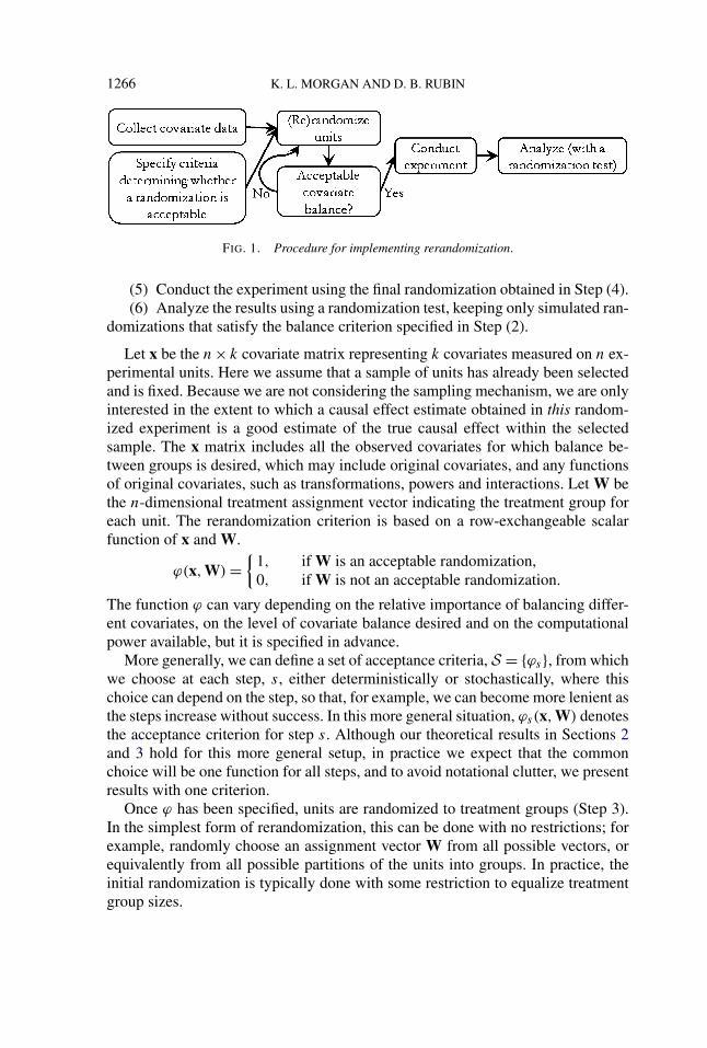
2.1. Procedure. The procedure for implementing rerandomization is depictedin Figure 1, and has the following steps:

(1) Collect covariate data.(2) Specify a balance criterion determining when a randomization is accept-

able.(3) Randomize the units to treatment groups.(4) Check the balance criterion; if the criterion is met, go to Step (5). Other-

wise, return to Step (3).


FIG. 1. Procedure for implementing rerandomization.

(5) Conduct the experiment using the final randomization obtained in Step (4).(6) Analyze the results using a randomization test, keeping only simulated ran-

domizations that satisfy the balance criterion specified in Step (2).

Let x be the n× k covariate matrix representing k covariates measured on n ex-perimental units. Here we assume that a sample of units has already been selectedand is fixed. Because we are not considering the sampling mechanism, we are onlyinterested in the extent to which a causal effect estimate obtained in this random-ized experiment is a good estimate of the true causal effect within the selectedsample. The x matrix includes all the observed covariates for which balance be-tween groups is desired, which may include original covariates, and any functionsof original covariates, such as transformations, powers and interactions. Let W bethe n-dimensional treatment assignment vector indicating the treatment group foreach unit. The rerandomization criterion is based on a row-exchangeable scalarfunction of x and W.

ϕ(x,W) ={

1, if W is an acceptable randomization,0, if W is not an acceptable randomization.

The function ϕ can vary depending on the relative importance of balancing differ-ent covariates, on the level of covariate balance desired and on the computationalpower available, but it is specified in advance.

More generally, we can define a set of acceptance criteria, S = {ϕs}, from whichwe choose at each step, s, either deterministically or stochastically, where thischoice can depend on the step, so that, for example, we can become more lenient asthe steps increase without success. In this more general situation, ϕs(x,W) denotesthe acceptance criterion for step s. Although our theoretical results in Sections 2and 3 hold for this more general setup, in practice we expect that the commonchoice will be one function for all steps, and to avoid notational clutter, we presentresults with one criterion.

Once ϕ has been specified, units are randomized to treatment groups (Step 3).In the simplest form of rerandomization, this can be done with no restrictions; forexample, randomly choose an assignment vector W from all possible vectors, orequivalently from all possible partitions of the units into groups. In practice, theinitial randomization is typically done with some restriction to equalize treatmentgroup sizes.


Rerandomization is simply a tool that allows us to draw from some predeter-mined set of acceptable randomizations, {W | ϕ(x,W) = 1}. Rerandomization isanalogous to rejection sampling; a way to draw from a set that may be tediousto enumerate. Specifying a set of acceptable randomizations and then choosingrandomly from this set is recommended by Kempthorne (1955, 1986) and Tukey(1993), and Moulton (2004) notes that rerandomization may be required for im-plementation of this idea when the set of acceptable randomizations is difficult toenumerate a priori.

Within this framework, rerandomization simply generalizes classical experi-mental designs. For the basic completely randomized experiment with fixed sam-ple sizes in each treatment group, ϕ(x,W) = 1 when the number of units assignedto each group matches the predetermined group sizes. For a randomized block ex-periment, ϕ(x,W) = 1 when predetermined numbers of units within each blockare assigned to each treatment group. For a Latin square, ϕ(x,W) = 1 when therandomization satisfies the Latin square design. These classical designs can bereadily sampled from, so rerandomization is computationally inefficient, althoughequivalent, but for other functions, ϕ, rerandomization may be a more straight-forward technique. Rerandomization can also be used together with any classicaldesign. For example, in a medical experiment on hypertensive drugs, we may blockon sex and a coarse categorization of baseline blood pressure, and use rerandom-ization to balance the remaining covariates, including fine baseline blood pressure.

Researchers are free to chose any function ϕ, provided it is chosen in advance.Section 2.3 describes the conditions necessary to maintain general unbiasedness ofsimple point estimation, Section 3 recommends a particular class of functions andstudies theoretical properties of this choice and Section 4 discusses some reasonsfor choosing an affinely invariant ϕ.

2.2. Analysis by randomization tests. Under most forms of rerandomization,increasing balance in the covariates will typically create more precise estimatedtreatment effects, making traditional Gaussian distribution-based forms of analy-sis statistically too conservative. However, the final data can be analyzed using arandomization test, maintaining valid frequentist properties. As Fisher stated, “Itseems to have escaped recognition that the physical act of randomization . . . af-fords the means, in respect of any particular body of data, of examining a widerhypothesis in which no normality of distribution is implied” [Fisher (1935)]. Thisphysical act of randomization need not be pure randomization, but any randomiza-tion scheme that can be replicated when conducting the randomization test.

We are interested in the effect of treatment assignment, W, on an outcome, y.Let yi(Wi) denote the ith unit’s, {i = 1, . . . , n}, potential outcome under treat-ment assignment Wi , following the Rubin causal model [Rubin (1974)]. Althoughrerandomization can be applied to any number of treatment conditions, to conveyessential ideas most directly, we consider only two, and refer to these conditions


as treatment and control. Let

Wi ={

1, if treated,0, if control.

Let Yobs(W) denote the vector of observed outcome values:

Yobs,i = yi(1)Wi + yi(0)(1 − Wi),(1)

where for notational simplicity the subscript obs means obs(W). Under the sharpnull hypothesis of no treatment effect on any unit, yi(1) = yi(0) for every i, andthus the vector Yobs is the same for every treatment assignment W. Consequently,leaving Yobs fixed and simulating many acceptable randomization assignments,W, we can empirically create the distribution of any estimator, g(x,W,yobs), ifthe null hypothesis were true. To account for the rerandomization, each simulatedrandomization must also satisfy ϕ(x,W) = 1. Once the desired number of ran-domizations has been simulated, the proportion of simulated randomizations withestimated treatment effect as extreme or more extreme than that observed in the ex-periment is the p-value. Although a full permutation test (including all the accept-able randomizations) is necessary for an exact p-value, the number of simulatedrandomizations can be increased to provide a p-value with any desired level ofaccuracy. This test can incorporate whatever rerandomization procedure was used,will preserve the significance level of the test [Moulton (2004)] and works for anyestimator. Brillinger, Jones and Tukey (1978), Tukey (1993) and Rosenberger andLachin [(2002), Chapter 7] suggest using randomization tests to assess significancewhen restricted randomization schemes are used.

Because analysis by a randomization test requires generating many acceptablerandomizations, computational time can be important to consider in advance. De-fine pa ≡ P(ϕ = 1) to be the proportion of acceptable randomizations. The choiceof pa involves a trade-off between better balance and computational time; smallervalues of pa ensure better balance, but they also imply a longer expected waitingtime to obtain an acceptable randomization, at least without clever computationaldevices. The number of randomizations required to get one acceptable randomiza-tion follows a geometric distribution with parameter pa , so N simulated acceptablerandomizations for a randomization test will require on average N/pa randomiza-tions to be generated.

The chosen pa must leave enough acceptable randomizations to perform a ran-domization test. In practice this is rarely an issue, because the number of possiblerandomizations is huge even for modest n. To illustrate, the number of possiblerandomizations for n = {30,50,100} randomizing to two equally sized treatmentgroups,

( nn/2

), is on the order of {108,1014,1029}, respectively. However, for small

sample sizes, care should be taken to ensure the number of acceptable randomiza-tions does not become too small, for example, less than 1000.

By employing the duality between confidence intervals and tests, for additivetreatment effects a confidence interval can be produced from a randomization dis-tribution as the set of all values for which the observed data would not reject


such a null hypothesized value [Lehmann and Romano (2005); Manly (2007),Section 3.5, Section 1.4]. Garthwaite (1996) provides an efficient algorithm forgenerating a confidence interval for additive effects from a randomization test.The assumption of additivity is statistically conservative, at least asymptotically,as implied by Neyman’s [Splawa-Neyman (1990)] results on standard errors beingoverestimated when assuming it relative to the actual standard errors. A random-ization test can be applied to any sharp null hypothesis, that is, a hypothesis suchthat the observed data implies specific values for all missing potential outcomes.

When the covariates being balanced are correlated with the outcome variable,then rerandomization increases precision (Section 3.2). A randomization test re-flects this increase in precision. Standard asymptotic-based frequentist analysisprocedures that do not take the rerandomization into account will be statisticallyconservative. Not only will distribution-based standard errors not incorporate theincrease in precision, but the act of rerandomizing itself will increase the estimatedstandard error beyond that of pure randomization. If the total variance in the out-come is fixed, decreasing the actual sampling variance between treatment groupmeans (by ensuring better balance), increases the variance within groups, and itis this variance within groups that is traditionally used to estimate the standarderror [Fisher (1926)]. Thus, although rerandomization decreases the true standarderror, it actually increases the standard error as estimated by traditional methods.For both of these reasons, the regular estimated standard errors will overestimatethe true standard error, and using the corresponding distribution-based methods ofanalysis after rerandomization results in overly wide confidence intervals and lesspowerful tests of hypotheses.

2.3. Maintaining an unbiased estimate. Although not needed to motivatererandomization, we assume one goal is to estimate the average treatment effect

τ ≡ y(1) − y(0)(2)

=∑n

i=1 yi(1)

n−

∑ni=1 yi(0)

n.

The fundamental problem in causal inference is that, because we only observeyi(Wi) for each unit, we cannot calculate (2) directly, and we must estimate τ usingonly Yobs . In this section, we assume the Stable Unit Treatment Value Assumption(SUTVA) [Rubin (1980)]: the potential outcomes are fixed and do not change withdifferent possible assignment vectors W.

The average treatment effect τ is usually estimated by the difference in observedsample means,

τ ≡ Yobs,T − Yobs,C,

where

Yobs,T ≡∑

i=1 Wiyi(1)∑ni=1 Wi

and Yobs,C ≡∑n

i=1(1 − Wi)yi(0)∑ni=1(1 − Wi)

.


THEOREM 2.1. Suppose∑n

i=1 Wi = ∑ni=1(1 − Wi) and ϕ(x,W) = ϕ(x,

1 − W); then E(τ | x, ϕ = 1) = τ .

PROOF. Under the specified conditions, W and 1 − W are exchangeable.Therefore, after rerandomization E(Wi | x, ϕ = 1) = E(1 − Wi | x, ϕ = 1) ∀i, soE(Wi | x, ϕ = 1) = E(1 − Wi | x, ϕ = 1) = 1/2 ∀i. Hence

E(τ | x, ϕ = 1) = E

(∑ni=1 WiYi,obs

n/2−

∑ni=1(1 − Wi)Yi,obs

n/2

∣∣∣ x, ϕ = 1)

= E

(∑ni=1 Wiyi(1)

n/2−

∑ni=1(1 − Wi)yi(0)

n/2

∣∣∣ x, ϕ = 1)

=∑n

i=1 E(Wi | ϕ = 1)yi(1)

n/2−

∑ni=1(1 − E(Wi | x, ϕ = 1))yi(0)

n/2

=∑n

i=1(1/2)yi(1)

n/2−

∑ni=1(1/2)yi(0)

n/2= τ. �

Theorem 2.1 holds for all outcome variables. Corollary 2.2 follows by the samelogic.

COROLLARY 2.2. If∑n

i=1 Wi = ∑ni=1(1 − Wi) and ϕ(x,W) = ϕ(x,1 − W),

then E(V T − V C | x, ϕ = 1) = 0 for any observed or unobserved covariate V .

If sample sizes are not fixed in advance, but each unit has E(Wi | x) = 1/2 in theinitial randomization, τ is only necessarily an unbiased estimate under the assump-tion of additivity. As a small example under nonadditivity, consider x = (0,1,2),y(1) = (1,1,0) and y(0) = (0,0,1). When ϕ(x,W) = 1 if the difference in x

means between the two groups is 0 and ϕ = 0 otherwise, the only two accept-able randomizations are W = (0,1,0) and W = (1,0,1). For either acceptablerandomization, τ = 1/2, yet τ = 1/3. This artificial example also illustrates thatif the treatment groups are of unequal size, τ will not necessarily be an unbiasedestimate after rerandomization. If the treatment group includes two units and thecontrol group one unit, and ϕ(x,W) is the same as before, then the only acceptablerandomization is W = (1,0,1), and once again, τ = 1/2, whereas τ = 1/3.

3. Rerandomization using Mahalanobis distance. To simplify the state-ment of theoretical results, we assume the sample sizes for the treatment and con-trol groups are fixed in advance, with pw the fixed proportion of treated units,

pw =∑n

i=1 Wi

n.(3)


Let XT − XC be the k-dimensional vector of the difference in covariate meansbetween the treatment and control groups,

XT − XC = x′Wnpw

− x′(1 − W)

n(1 − pw)= x′(W − pw1)

npw(1 − pw).(4)

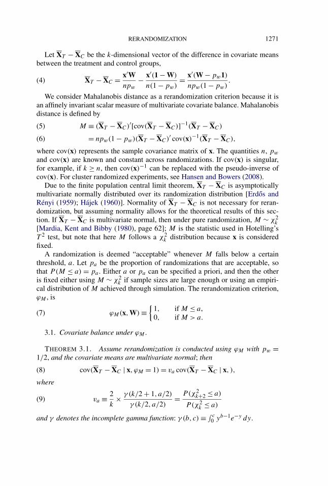
We consider Mahalanobis distance as a rerandomization criterion because it isan affinely invariant scalar measure of multivariate covariate balance. Mahalanobisdistance is defined by

M ≡ (XT − XC)′[cov(XT − XC)]−1(XT − XC)(5)

= npw(1 − pw)(XT − XC)′ cov(x)−1(XT − XC),(6)

where cov(x) represents the sample covariance matrix of x. The quantities n, pw

and cov(x) are known and constant across randomizations. If cov(x) is singular,for example, if k ≥ n, then cov(x)−1 can be replaced with the pseudo-inverse ofcov(x). For cluster randomized experiments, see Hansen and Bowers (2008).

Due to the finite population central limit theorem, XT − XC is asymptoticallymultivariate normally distributed over its randomization distribution [Erdos andRényi (1959); Hájek (1960)]. Normality of XT − XC is not necessary for reran-domization, but assuming normality allows for the theoretical results of this sec-tion. If XT − XC is multivariate normal, then under pure randomization, M ∼ χ2

k

[Mardia, Kent and Bibby (1980), page 62]; M is the statistic used in Hotelling’sT 2 test, but note that here M follows a χ2

k distribution because x is consideredfixed.

A randomization is deemed “acceptable” whenever M falls below a certainthreshold, a. Let pa be the proportion of randomizations that are acceptable, sothat P(M ≤ a) = pa . Either a or pa can be specified a priori, and then the otheris fixed either using M ∼ χ2

k if sample sizes are large enough or using an empiri-cal distribution of M achieved through simulation. The rerandomization criterion,ϕM , is

ϕM(x,W) ≡{

1, if M ≤ a,0, if M > a.

(7)

3.1. Covariate balance under ϕM .

THEOREM 3.1. Assume rerandomization is conducted using ϕM with pw =1/2, and the covariate means are multivariate normal; then

cov(XT − XC | x, ϕM = 1) = va cov(XT − XC | x, ),(8)

where

va ≡ 2

k× γ (k/2 + 1, a/2)

γ (k/2, a/2)= P(χ2

k+2 ≤ a)

P (χ2k ≤ a)

(9)

and γ denotes the incomplete gamma function: γ (b, c) ≡ ∫ c0 yb−1e−y dy.


FIG. 2. The percent reduction in variance for each covariate difference in means, as a function ofthe number of covariates and the proportion of randomizations accepted.

The proof of Theorem 3.1 is in the Appendix.In the field of matching, emphasis has been placed on “percent reduction in

bias” [Cochran and Rubin (1973)]. In the context of randomized experiments thereis no bias, and rerandomization instead reduces the sampling variance of the dif-ference in covariate means, yielding differences that are more closely concentratedaround 0. Define the percent reduction in variance, the percentage by which reran-domization reduces the randomization variance of the difference in means, for eachcovariate, xj , by

100(

var(Xj,T − Xj,C | x) − var(Xj,T − Xj,C | x, ϕ = 1)

var(Xj,T − Xj,C | x)

).(10)

By Theorem 3.1, the percent reduction in variance for each covariate, and for anylinear combination of these covariates, is

100(1 − va)(11)

and is shown as a function of k and pa in Figure 2, where by (9), 0 ≤ va ≤ 1.The lower the acceptance probability and the fewer covariates being balanced, thelarger the percent reduction in variance.

Notice that Theorem 3.1 holds for any covariate distribution, as long as the sam-ple size is large enough for the central limit theorem to ensure normally distributedcovariate means. An exact value is not needed, and an estimate is used only toguide the choice of pa ; it has no influence on the validity of resulting inferences.


3.2. Precision of the estimated treatment effect. Rerandomization improvesprecision, provided the outcome and covariates are correlated. Thus researcherscan increase the power of tests and decrease the width of confidence intervalssimply at the expense of computational time.

THEOREM 3.2. If (a) rerandomization is conducted using ϕM with pw = 1/2,(b) the covariate and outcome means are normally distributed, and (c) the treat-ment effect is additive, then the percent reduction in variance of τ is

100(1 − va)R2,(12)

where R2 represents the squared multiple correlation between y and x within atreatment group and va is as defined in (9).

PROOF. Regardless of the true relationship between the outcome and covari-ates, by additivity we can write

yi(Wi) | xi = β0 + β ′xi + τWi + ei,(13)

where β0 + β ′xi is the projection of yi onto the space spanned by (1,x), and ei

is a residual that encompasses any deviations from the linear model. Then theestimated treatment effect, τ , can be expressed as

τ = β ′(XT − XC) + τ + (eT − eC).(14)

Because τ is constant and the first and last terms are uncorrelated, we can expressthe variance of τ as

var(τ ) = var(β ′(XT − XC)

) + var(eT − eC)(15)

= β ′ cov(XT − XC)β + var(eT − eC).

By Theorem 3.1, rerandomization modifies the first term by the factor va . Becauseunder normality, orthogonality implies independence, the difference in residualmeans is independent of the difference in covariate means, and thus rerandomiza-tion has no affect on the second term. Therefore, the variance of τ after rerandom-ization restricting M ≤ a is

var(τ | x,M ≤ a) = β ′ cov(XT − XC | x,M ≤ a)β + var(eT − eC | x,M ≤ a)(16)

= vaβ′ cov(XT − XC | x)β + var(eT − eC | x).

Let σ 2e be the variance of the residuals and σ 2

y be the variance of the outcomewithin each treatment group, where σ 2

e = σ 2y (1 − R2). Thus

var(eT − eC | x) = σ 2e

npw(1 − pw)= σ 2

y (1 − R2)

npw(1 − pw),(17)


and

β ′ cov(XT − XC | x)β = var(τ | x) − var(eT − eC | x)

= σ 2y − σ 2

e

npw(1 − pw)(18)

= σ 2y R2

npw(1 − pw).

Therefore by (16), (17) and (18), the variance of τ after rerandomization is

var(τ | x,M ≤ a) = vaβ′ cov(XT − XC | x)β + var(eT − eC | x)

= vaσ2Y R2

npw(1 − pw)+ σ 2

Y (1 − R2)

npw(1 − pw)

= (1 − (1 − va)R

2) σ 2Y

npw(1 − pw)

= (1 − (1 − va)R

2)var(τ | x).

Thus the percent reduction in variance is 100(1 − (1 − (1 − va)R2) = 100(1 −

va)R2. �

The percent reduction in variance for the estimated treatment effect, shown as afunction of k, pa and R2 in Figure 3, is simply the percent reduction in variance foreach covariate, scaled by R2. Because under the specified conditions τ is unbiased

FIG. 3. The percent reduction in variance for the estimated treatment effect, as a function of theacceptance probability, the number of covariates, and R2.


by Theorem 2.1, 100(1 − va)R2 is not only the percent reduction in variance in

the estimated treatment effect, but also the percent reduction in mean square error(MSE).

If regression (i.e., analysis of covariance) is used to adjust for imbalance in acompletely randomized experiment, the percent reduction in variance is

100[(

1 + M

n

)R2 − M

n

](19)

[Cox (1982)], where M is as in (6). Comparing (19) to (10), we see that rerandom-ization can increase precision more than regression adjustment because there is noestimation of regression coefficients with the former. Note that the highest percentreduction in variance achievable by either rerandomization or regression is 100R2,achieved with perfect covariate mean balance.

4. Affinely invariant rerandomization criteria. In this section we explorethe theoretical implications of choosing an affinely invariant rerandomizationcriterion, meaning that for any affine transformation of x, a + bx, ϕ(x,W) =ϕ(a +bx,W). Measures based on inner products, such as Mahalanobis distance orthe estimated best linear discriminant, are affinely invariant, as are criteria basedon propensity scores estimated by linear logistic regression [Rubin and Thomas(1992)]. Results in this section parallel those for affinely invariant matching meth-ods [Rubin and Thomas (1992)].

In the previous sections, we regarded x as fixed, and only the randomizationvector, W was random. In this section, to use ellipsoidal symmetry of x, we regardboth x and W as random, so expectations are over repeated draws of x and repeatedrandomizations.

THEOREM 4.1. If ϕ is affinely invariant, and if x is ellipsoidally symmetric,then

E(XT − XC | ϕ = 1) = E(XT − XC) = 0 and(20)

cov(XT − XC | ϕ = 1) ∝ cov(XT − XC).(21)

PROOF. First, by ellipsoidal symmetry there is an affine transformation of xto a canonical form with mean (center) zero and covariance (inner product) I,the k-dimensional identity matrix. The distribution of the matrix x in the treatedgroup of size npw and the control group of size n(1 − pw) are both independentand identically distributed samples from this zero centered spherical distribution.Any affinely invariant rule for selecting subsets of treated and control units will bea function of affinely invariant statistics in the treatment and control groups thatare also zero-centered spherically symmetric. Applying ϕ creates concentric zero-centered sphere(s) that partition the space of these statistics into regions where ϕ =1 and ϕ = 0, and therefore the distribution of such statistics remains zero-centered


and spherically symmetric. Transforming back to the original form completes theproof. �

COROLLARY 4.2. If ϕ is affinely invariant and if x is ellipsoidally symmetric,then rerandomization leads to unbiased estimates of any linear function of x.

Note that, unlike Corollary 2.2, Corollary 4.2 applies no matter how the samplesizes are chosen.

COROLLARY 4.3. If ϕ is affinely invariant and if x is ellipsoidally symmetric,then

cor(XT − XC | ϕ = 1) = cor(XT − XC).(22)

One possible method of rerandomization, suggested by Moulton (2004),Maclure et al. (2006), Bruhn and McKenzie (2009) and Cox (2009), is to placebounds separately on each entry of XT − XC and ensure that each covariate differ-ence is within its specified caliper. However, this method is not affinely invariantand will generally destroy the correlational structure of XT − XC , even when x isellipsoidally symmetric.

Analogous to “Equal Percent Bias Reducing” (EPBR) matching methods[Rubin (1976)], a rerandomization method is said to be “Equal Percent VarianceReducing” (EPVR) if the percent reduction in variance is the same for each co-variate.

COROLLARY 4.4. If ϕ is affinely invariant and if x is ellipsoidally symmetric,then rerandomization is EPVR for x and any linear function of x.

Rerandomization methods that are not affinely invariant could increase the vari-ance of some linear combinations of covariates [Rubin (1976)].

Although affinely invariant methods have desirable properties in general, theyare not always preferred. For example, if covariates are known to vary in impor-tance, a rerandomization method that is not EPVR may be more desirable, allowinggreater percent reduction in variance for more important covariates. Rerandomiza-tion criteria that take into account covariates of varying importance are discussedin Lock [(2011), Chapter 4].

5. Discussion.

5.1. Alternatives for balancing covariates. Rerandomization is certainly notthe only way to balance covariates before the experiment.

With only a few categorical covariates, simple blocking can successfully bal-ance all covariates, and there is no need for rerandomization. With many covariates


each taking on many values, however, blocking on all covariates can be impossi-ble, and in this case we recommend blocking on the most important covariates,and rerandomizing to balance the components of the covariates orthogonal to theblocks. Blocking and rerandomization can, and we feel should, be used together.Multivariate matching [Greevy et al. (2004); Rubin (2006); Ho et al. (2007); Imai,King and Nall (2009); Xu and Kalbfleisch (2010)] is a special case of blockingthat can better handle many covariates.

Restricted (or constrained) randomization [Yates (1948); Grundy and Healy(1950); Youden (1972); Bailey (1983)] restricts the set of acceptable randomiza-tions in a way that preserves the validity of asymptotic-based distributional meth-ods of analysis. However, most work on restricted randomization is specific to agri-cultural plots, and apparently has not been extended to multiple covariates. Block-ing, matching and restricted randomization can all also be implemented throughrerandomization by specifying the set of acceptable randomizations through ϕ.

The Finite Selection Model (FSM) [Morris (1979); Morris and Hill (2000)] pro-vides balance for multiple covariates, but provides a fixed amount of balance in afixed amount of computational time. Rerandomization has the flexibility to choosethe desired tradeoff between balance and computational time. More details com-paring FSM with rerandomization are in [Lock (2011), Section 5.5].

Covariate-adaptive randomization schemes [Efron (1971); White and Freed-man (1978); Pocock and Simon (1975); Pocock (1979); Simon (1979); Birkett(1985); Aickin (2001); Atkinson (2002); Scott et al. (2002); McEntegart (2003);Rosenberger and Sverdlov (2008)] are designed for clinical trials with sequentialtreatment allocation over extended periods of time. Rerandomization as proposedhere is not applicable to sequential allocation, and instead readers interested insuch trials can refer to the above sources.

If covariates are not balanced before the experiment, post-hoc methods such asregression adjustment are commonly used, which rely on assumptions that oftencannot be verified [Tukey (1993); Freedman (2008)]. Moreover, unlike post-hocmethods, rerandomization is conducted entirely at the design stage, and so cannotbe influenced by outcome data. Tukey (1993) and Rubin (2008b) give convincingreasons for why as much as possible should be done in the design phase of an ex-periment, before outcome data are available, rather than in the analysis stage whenthe researcher has the potential to bias the results, consciously or unconsciously.

5.2. Extensions and additional considerations. For multiple treatment groups,any of the test statistics commonly used in multivariate analysis of variance(MANOVA) can be used to measure balance. The standard statistics are all equiv-alent to Mahalanobis distance in the special case of two groups. Extensions formultiple treatment groups are discussed in Lock [(2011), Section 5.2].

For unbiased estimates using rerandomization with treatment groups of unequalsizes, multiple treatment groups of equal size can be created, and then merged asneeded after the rerandomization procedure, but before the physical experiment. If


extra units are discarded to form equal sized treatment groups and rerandomizationis employed, precision can actually increase if covariates are highly correlated withthe outcome [Lock (2011), Section 5.3].

In a Bayesian analysis, as long as all covariates relevant to ϕ(x,W) are condi-tioned on, the design is ignorable [Rubin (1978)], and theoretically, the analysiscan proceed as usual.

6. Conclusion. Randomization balances covariates across treatment groups,but only on average, and in any one experiment covariates may be unbalanced.Rerandomization provides a simple and intuitive way to improve covariate balancein randomized experiments.

To perform rerandomization, a criterion determining whether a randomizationis acceptable needs to be specified. For unbiasedness, this rule needs to be sym-metric regarding the treatment groups. If the criterion is affinely invariant, thenfor ellipsoidally symmetric distributions, balance improvement will be the samefor all covariates (and all linear combinations of the covariates), and correlationsbetween covariate differences in means will be maintained. One such criterion isto rerandomize whenever Mahalanobis distance exceeds a certain threshold.

When the covariates are correlated with the outcome, rerandomization increasesprecision. If the analysis reflects the rerandomization procedure, this leads to moreprecise estimates, more powerful tests and narrower confidence intervals.

APPENDIX

PROOF OF THEOREM 3.1. Because M ∼ χ2k under pure randomization when

the covariate means are normally distributed, rerandomization affects the mean ofM as follows:

E(M | x,M ≤ a) = (1/((k/2)2k/2))∫ a

0 yk/2e−y/2 dy

(1/((k/2)2k/2))∫ a

0 yk/2−1e−y/2 dy

=∫ a

0 (y/2)k/2e−y/2 dy

(1/2)∫ a

0 (y/2)k/2−1e−y/2 dy(23)

= 2 × γ (k/2 + 1, a/2)

γ (k/2, a/2).

To prove (8), we convert the covariates to canonical form [Rubin and Thomas(1992)]. Let � = cov(XT − XC | x), and define

Z ≡ �−1/2(XT − XC),(24)

where �−1/2 is the Cholesky square root of −1, so �−1/2′�−1/2 = �−1. By the

assumption of normality,

Z | x ∼ Nk(0, I).


Due to normality, uncorrelated implies independent and thus the elements of Z areindependent and identically distributed (i.i.d.) standard normals. Therefore, theelements of Z are exchangeable.

By (5), M = Z′Z = ∑kj=1 Z2

j . Therefore for each j we have

var(Zj | x,M ≤ a) = E(Z2j | x,M ≤ a)

= E(M | x,M ≤ a)

k(25)

= 2

k× γ (k/2 + 1, a/2)

γ (k/2, a/2)

= va,(26)

where (25) follows from the exchangeability of the elements of Z.After enforcing M ≤ a, the elements of Z are no longer independent (they will

be negatively correlated in magnitude), but with signs they remain uncorrelateddue to symmetry:

cov(Zi,Zj | x,M ≤ a) = E(ZiZj | x,M ≤ a)

− E(Zi | x,M ≤ a)E(Zj | x,M ≤ a)

= E(E(ZiZj | Zj ,x,M ≤ a) | x,M ≤ a

) − 0(27)

= E(ZjE(Zi | Zj ,x,M ≤ a) | x,M ≤ a

)= E(Zj × 0 | x,M ≤ a)(28)

= 0,(29)

where (27) follows from Corollary 2.2, and (28) follows because (Zi | Zj ,M ≤a) ∼ (−Zi | Zj ,M ≤ a), thus E(Zi | Zj ,M ≤ a) = 0 for all i, j .

Thus after rerandomization the covariance matrix of Z is vaI, hence

cov(XT − XC | x,M ≤ a) = cov(�1/2Z | x,M ≤ a)

= �1/2 cov(Z | x,M ≤ a)�1/2′

= va�

= va cov(XT − XC | x). �

Acknowledgments. We appreciate the extraordinarily helpful comments ofthe editor, Professor Bühlmann, and two reviewers.

REFERENCES

AICKIN, M. (2001). Randomization, balance, and the validity and efficiency of design-adaptive al-location methods. J. Statist. Plann. Inference 94 97–119. MR1820173

http://www.ams.org/mathscinet-getitem?mr=1820173


ANSCOMBE, F. J. (1948a). The validity of comparative experiments. J. Roy. Statist. Soc. Ser. A. 111181–211. MR0030181

ARNOLD, G. C. (1986). Randomization: A historic controversy. In The Fascination of Statistics(R. J. Brook, G. C. Arnold, T. H. Hassard and R. M. Pringle, eds.) 231–244. CRC Press, BocaRaton, FL.

ATKINSON, A. C. (2002). The comparison of designs for sequential clinical trials with covariateinformation. J. Roy. Statist. Soc. Ser. A 165 349–373. MR1904822

BAILEY, R. A. (1983). Restricted randomization. Biometrika 70 183–198. MR0742988BAILEY, R. A. (1986). Randomization, constrained. Encyclopedia of Statistical Sciences 7 519–524.BAILEY, R. A. and ROWLEY, C. A. (1987). Valid randomization. Proc. R. Soc. Lond. Ser. A Math.

Phys. Eng. Sci. 410 105–124.BIRKETT, N. J. (1985). Adaptive allocation in randomized controlled trials. Control Clin Trials 6

146–155.BRILLINGER, D., JONES, L. and TUKEY, J. (1978). The Management of Weather Resources II: The

Role of Statistics in Weather Resources Management. US Government Printing Office, Washing-ton, DC.

BRUHN, M. and MCKENZIE, D. (2009). In pursuit of balance: Randomization in practice in devel-opment field experiments. American Economic Journal: Applied Economics 1 200–232.

COCHRAN, W. G. and RUBIN, D. B. (1973). Controlling bias in observational studies: A review.Sankhya Ser. A 35 417–446.

COX, D. R. (1982). Randomization and concomitant variables in the design of experiments. InStatistics and Probability: Essays in Honor of C. R. Rao 197–202. North-Holland, Amsterdam.MR0659470

COX, D. R. (2009). Randomization in the Design of Experiments. International Statistical Review77 415–429.

EFRON, B. (1971). Forcing a sequential experiment to be balanced. Biometrika 58 403–417.MR0312660

ERDOS, P. and RÉNYI, A. (1959). On the central limit theorem for samples from a finite population.Magyar Tud. Akad. Mat. Kutató Int. Közl. 4 49–61. MR0107294

FISHER, R. A. (1926). The arrangement of field experiments. Journal of the Ministry of Agricultureof Great Britain 33 503–513.

FISHER, R. A. (1935). The Design of Experiments. Oliver and Boyd, Edinburgh.FREEDMAN, D. A. (2008). On regression adjustments to experimental data. Adv. in Appl. Math. 40

180–193. MR2388610GARTHWAITE, P. H. (1996). Confidence intervals from randomization tests. Biometrics 1387–1393.GOSSET, W. J. (1938). Comparison between balanced and random arrangements of field plots.

Biometrika 29 363.GREENBERG, B. G. (1951). Why randomize? Biometrics 7 309–322.GREEVY, R., LU, B., SILBER, J. H. and ROSENBAUM, P. (2004). Optimal multivariate matching

before randomization. Biostatistics 5 263–275.GRUNDY, P. M. and HEALY, M. J. R. (1950). Restricted randomization and quasi-Latin squares.

J. R. Stat. Soc. Ser. B Stat. Methodol. 12 286–291.HÁJEK, J. (1960). Limiting distributions in simple random sampling from a finite population. Mag-

yar Tud. Akad. Mat. Kutató Int. Közl. 5 361–374. MR0125612HANSEN, B. B. and BOWERS, J. (2008). Covariate balance in simple, stratified and clustered com-

parative studies. Statist. Sci. 23 219–236. MR2516821HARVILLE, D. A. (1975). Experimental randomization: Who needs it? Amer. Statist. 27–31.HO, D. E., IMAI, K., KING, G. and STUART, E. A. (2007). Matching as nonparametric preprocess-

ing for reducing model dependence in parametric causal inference. Political Analysis 15 199–236.HOLSCHUH, N. (1980). Randomization and design: I. In R. A. Fisher: An Appreciation (S. E. Fien-

berg and D. V. Hinkley, eds.). Lecture Notes in Statistics 1 35–45. Springer, New York.











IMAI, K., KING, G. and STUART, E. A. (2008). Misunderstanding between experimentalists andobservationalists about causal inference. J. Roy. Statist. Soc. Ser. A 171 481–502. MR2427345

IMAI, K., KING, G. and NALL, C. (2009). The essential role of pair matching in cluster-randomizedexperiments, with application to the Mexican universal health insurance evaluation. Statist. Sci.24 29–53. MR2561126

KEELE, L., MCCONNAUGHY, C., WHITE, I., LIST, P. M. E. M. and BAILEY, D. (2009). Adjustingexperimental data. In Experiments in Political Science Conference.

KEMPTHORNE, O. (1955). The randomization theory of experimental inference. J. Amer. Statist.Assoc. 50 946–967. MR0071696

KEMPTHORNE, O. (1986). Randomization II. Encyclopedia of Statistical Sciences 7 519–524.KRAUSE, M. S. and HOWARD, K. I. (2003). What random assignment does and does not do. Journal

of Clinical Psychology 59 751–766.LEHMANN, E. L. and ROMANO, J. P. (2005). Testing Statistical Hypotheses, 3rd ed. Springer Texts

in Statistics. Springer, New York. MR2135927LOCK, K. F. (2011). Rerandomization to improve covariate balance in randomized experiments

Ph.D. thesis, Harvard Univ., Cambridge, MA.MACLURE, M., NGUYEN, A., CARNEY, G., DORMUTH, C., ROELANTS, H., HO, K. and

SCHNEEWEISS, S. (2006). Measuring prescribing improvements in pragmatic trials of educa-tional tools for general practitioners. Basic & Clinical Pharmacology & Toxicology 98 243–252.

MANLY, B. F. J. (2007). Randomization, Bootstrap and Monte Carlo Methods in Biology, 3rd ed.Chapman & Hall/CRC, Boca Raton, FL. MR2257066

MARDIA, K. V., KENT, J. T. and BIBBY, J. M. (1980). Multivariate Analysis. Academic Press,London. MR0560319

MCENTEGART, D. J. (2003). The pursuit of balance using stratified and dynamic randomizationtechniques: An overview. Drug Information Journal 37 293–308.

MORRIS, C. (1979). A finite selection model for experimental design of the health insurance study.J. Econometrics 11 43–61.

MORRIS, C. N. and HILL, J. L. (2000). The health insurance experiment: Design using the finiteselection model. In Public Policy and Statistics: Case Studies from RAND 29–53. Springer, NewYork.

MOULTON, L. H. (2004). Covariate-based constrained randomization of group-randomized trials.Clin Trials 1 297–305.

POCOCK, S. J. (1979). Allocation of patients to treatment in clinical trials. Biometrics 35 183–197.POCOCK, S. J. and SIMON, R. (1975). Sequential treatment assignment with balancing for prognos-

tic factors in the controlled clinical trial. Biometrics 31 103–115.RAYNOR, A. A. (1986). Some Sidelights on Experimental Design. In The Fascination of Statistics

(R. J. Brook, G. C. Arnold, T. H. Hassard and R. M. Pringle, eds.) 245–264. CRC Press, BocaRaton, FL.

ROSENBERGER, W. F. and LACHIN, J. M. (2002). Randomization in Clinical Trials: Theory andPractice. Wiley, New York. MR1914364

ROSENBERGER, W. F. and SVERDLOV, O. (2008). Handling covariates in the design of clinicaltrials. Statist. Sci. 23 404–419. MR2483911

RUBIN, D. B. (1974). Estimating causal effects of treatments in randomized and nonrandomizedstudies. Journal of Educational Psychology 66 688.

RUBIN, D. B. (1976). Multivariate matching methods that are equal percent bias reducing. I. Someexamples. Biometrics 32 109–120. MR0400555

RUBIN, D. B. (1978). Bayesian inference for causal effects: The role of randomization. Ann. Statist.6 34–58. MR0472152

RUBIN, D. B. (1980). Randomization analysis of experimental data: The Fisher randomization testcomment. J. Amer. Statist. Assoc. 75 591–593.












RUBIN, D. B. (2006). Matched Sampling for Causal Effects. Cambridge Univ. Press, Cambridge.MR2307965

RUBIN, D. B. (2008a). Comment: The design and analysis of gold standard randomized experiments.J. Amer. Statist. Assoc. 103 1350–1353. MR2655717

RUBIN, D. B. (2008b). For objective causal inference, design trumps analysis. Ann. Appl. Stat. 2808–804. MR2516795

RUBIN, D. B. and THOMAS, N. (1992). Affinely invariant matching methods with ellipsoidal distri-butions. Ann. Statist. 20 1079–1093. MR1165607

SAVAGE, L. J. (1962). The Foundations of Statistical Inference. Methuen & Co. Ltd., London.MR0146908

SCOTT, N. W., MCPHERSON, G. C., RAMSAY, C. R. and CAMPBELL, M. K. (2002). The methodof minimization for allocation to clinical trials. a review. Control Clinical Trials 23 662–674.

SEIDENFELD, T. (1981). Levi on the dogma of randomization in experiments. In Henry E. Kyburg,Jr. & Isaac Levi (R. J. Bogdan, ed.) 263–291. Springer, Berlin.

SIMON, R. (1979). Restricted randomization designs in clinical trials. Biometrics 35 503–512.SOARES, J. F. and WU, C. F. J. (1985). Optimality of random allocation design for the control of

accidental bias in sequential experiments. J. Statist. Plann. Inference 11 81–87. MR0783375SPLAWA-NEYMAN, J. (1990). On the application of probability theory to agricultural experiments.

Essay on principles. Section 9. Statist. Sci. 5 465–472. MR1092986SPROTT, D. A. and FAREWELL, V. T. (1993). Randomization in experimental science. Statist. Pa-

pers 34 89–94. MR1221524TUKEY, J. W. (1993). Tightening the clinical trial. Control Clin Trials 14 266–285.URBACH, P. (1985). Randomization and the design of experiments. Philos. Sci. 52 256–273.

MR0804567WHITE, S. J. and FREEDMAN, L. S. (1978). Allocation of patients to treatment groups in a con-

trolled clinical study. British Journal of Cancer 37 849.WORRALL, J. (2010). Evidence: Philosophy of science meets medicine. J. Eval. Clin. Pract. 16

356–362.XU, Z. and KALBFLEISCH, J. D. (2010). Propensity score matching in randomized clinical trials.

Biometrics 66 813–823. MR2758217YATES, F. (1939). The comparative advantages of systematic and randomized arrangements in the

design of agricultural and biological experiments. Biometrika 30 440.YATES, F. (1948). Contribution to the discussion of “The validity of comparative experiments” by

FJ Anscombe. J. Roy. Statist. Soc. Ser. A 111 204–205.YOUDEN, W. J. (1972). Randomization and experimentation. Technometrics 14 13–22.

DEPARTMENT OF STATISTICS

DUKE UNIVERSITY

BOX 90251DURHAM, NORTH CAROLINA 27708USAE-MAIL: [email protected]

STATISTICS DEPARTMENT

HARVARD UNIVERSITY

1 OXFORD ST.CAMBRIDGE, MASSACHUSETTS 02138USAE-MAIL: [email protected]











mailto:[email protected]

mailto:[email protected]

rerandomization to improve covariate balance in experiments

Documents