research article eoq models with varying holding...
TRANSCRIPT

Hindawi Publishing CorporationJournal of Industrial MathematicsVolume 2013 Article ID 743921 7 pageshttpdxdoiorg1011552013743921
Research ArticleEOQ Models with Varying Holding Cost
Naser Ghasemi and Behrouz Afshar Nadjafi
Faculty of Industrial and Mechanical Engineering Islamic Azad University Qazvin Branch PO Box 34185-1416Qazvin 34185-14161 Iran
Correspondence should be addressed to Behrouz Afshar Nadjafi afsharnbalumsharifedu
Received 10 March 2013 Revised 23 April 2013 Accepted 7 May 2013
Academic Editor Ting Chen
Copyright copy 2013 N Ghasemi and B Afshar Nadjafi This is an open access article distributed under the Creative CommonsAttribution License which permits unrestricted use distribution and reproduction in any medium provided the original work isproperly cited
Models of inventory management contain different parameters An issue is observable in the classical models which can be relatedto the determination of the quantity of the economic order and the quantity of the economic production In these models theparameters like setup and holding costs and also the rate of demands are fixed This matter causes the quantity of the economicordering in classic model to have some differences in comparison with the real-world conditions It should be stated that holdingcost of spoiled and useless products is not always fixed and so the costs increase by passing the time This paper is an attempt todevelop classical EOQ models by considering holding cost as an increasing function of the ordering cycle length So the classicalEOQ models are developed and the related optimum quantity to the ordering cycle length economic ordering quantity and theoptimum total cost are determined
1 Introduction
Models of inventory management contain different param-eters An issue that is observable in the classical modelscan be related to the determination of the quantity of theeconomical ordering and the quantity of the economical pro-duction In these models the parameters like setup costholding cost and also the rate of demand are fixed Thismatter causes that the economic ordering quantity and theeconomic production quantity in classicmodels to have somedifferences in comparison with the real-world conditionsThus it seems necessary that the parameters assumptionsand limitations should be considered in amanner to approachthe real condition as much as possible [1]
It should be stated that the costs of holding spoiled anduseless products are not always fixed and similar and therate of cost is increased by passing the time Also the rateof holding costs which is related to rental equipment can getdiscounts for long-term usages and can be decreasing by timepassing [2]
The aim of this paper is to present somemodels similar tothe real-world conditions In this paper the related parame-ters to the holding cost are not considered as the fixed onesand it is regarded as the increasing function of the ordering
cycle length for determining the economic ordering cyclelength and the economic ordering quantity in two cases Thefirst case does not allow backorders and the other one permitsbackorders Itmeans that in a situationwhere the holding costis a function of the ordering cycle length we want to min-imize the total amount of the costs Holding cost should beconsidered as a kind of increasing function of ordering cyclelength and the optimum inventory cycle and economic orderquantity are decision variables
Inventory control models are used widely in differentfields for production and sale since the introduction of themodels on economic order quantity and economical produc-tion quantity Some researchers have questioned and investi-gated the practical usages of these models with reference tothe unreal assumptions as well as the parameters such assetup and holding costs and also the rate of demand Darwishdeveloped an EPQ classic model with reference to the setupcost as a function of production time [1] He suggested twomodels such that in the first model the shortages were notallowed and in the second model the shortages were allowedHe indicates that the function of cost is convex in both casesand the optimum quantity of the main function is observablein both models The results show that the relationshipbetween the cost function and the production time can have a
2 Journal of Industrial Mathematics
significant effect on the economical production quantity andthe average amount of the total cost in EPQ classic model
The holding cost in some fewmodels has been consideredas a variable one Alfares investigated the inventory policyfor an item with a stock-level-dependent demand rate anda storage-time-dependent holding cost [2] The holding costper unit of the item per unit time is assumed to be an increas-ing function of the time spent in storages Two time-depend-ent holding cost step functions are considered retroactiveholding cost increasing function and incremental holdingcost increasing function Procedures are developed for deter-mining the optimal order quantity and the optimal cycle timefor both cost structures
Giri et al developed a generalized EOQ model for deter-iorating items with shortages in which both the demand rateand the holding cost are continuous functions of time Theoptimal inventory policy is derived assuming a finite plan-ning horizon and constant replenishment cycles [3]
Ray and Chaudhuri take the time value of money intoaccount in analyzing an inventory systemwith stock-depend-ent demand rate and shortages Two types of inflation ratesare considered internal (company) inflation and external(general economy) inflation [4]
Goh developed a classic model for the fund relateddemand and the holding expense He considered the holdingcost in two forms In the first case it was in the shape of a non-linear function of time and the second case was in the shapeof a nonlinear function of inventory level [5] Baker andUrban developed a deterministic inventor system with aninventory-level-dependent rate [6] Barron considered eco-nomic production quantity with rework process at a single-stage manufacturing system with planned backorders [7]Hou considers an EPQ model with imperfect productionprocesses in which the setup cost and process quality arefunctions of capital expenditure [8] Pan et al developedoptimal reorder point inventory models with variable leadtime and backorder discount considerations [9] Sphicasconsidered EOQ and EPQ with linear and fixed backordercosts two cases identified and models analyzed withoutcalculus [10] Urban presented a comprehensive review andunifying theory for inventory models with inventory-level-dependent demand [11]
2 Problem Description
The main objective of this paper is developing classicalEOQ models with considering holding cost as an increasingcontinuous function of ordering cycle length
21 Assumptions Consider the following
(i) The rate of demand is fixed(ii) There is no discount(iii) The delivery of the product is wholesale(iv) All parameters are fixed and deterministic(v) Holding cost is an increasing function of period
length
22 Parameters Consider the following
119863 the rate of demands119876 the quantity of order (decision variable)119896 the cost of ordering or setup in the period of main
ordersℎ0 the constant unit holding cost before 1198791015840
119875 the rate of production (the rate of production import)119861 the quantity of backorder (decision variable)120587 the unit backorder cost per unit time119879 inventory cycle length
119879119862 annual total cost119879119874119862 annual setup cost119879119867119862 annual holding cost119879119878119862 annual backorder cost
3 Models Development
In this part EOQ models in two cases are developed in acondition where the holding cost is an increasing continuousfunction of ordering cycle length At first model backordersare not permitted and in second model backorders areallowed We assume that the holding cost will be fixed till adefinite time (1198791015840) and then will be increased according to afunction of ordering cycle length So for holding cost (ℎ) wehave
ℎ = ℎ0119879120576
119879 gt 1198791015840
ℎ0
119879 le 1198791015840
0 lt 120576 lt 1 (1)
where 1198791015840 is a time moment before which holding cost is
constant It is clear that in (1) while 120576 = 0 the presentedmodels will reflect the results of classic models
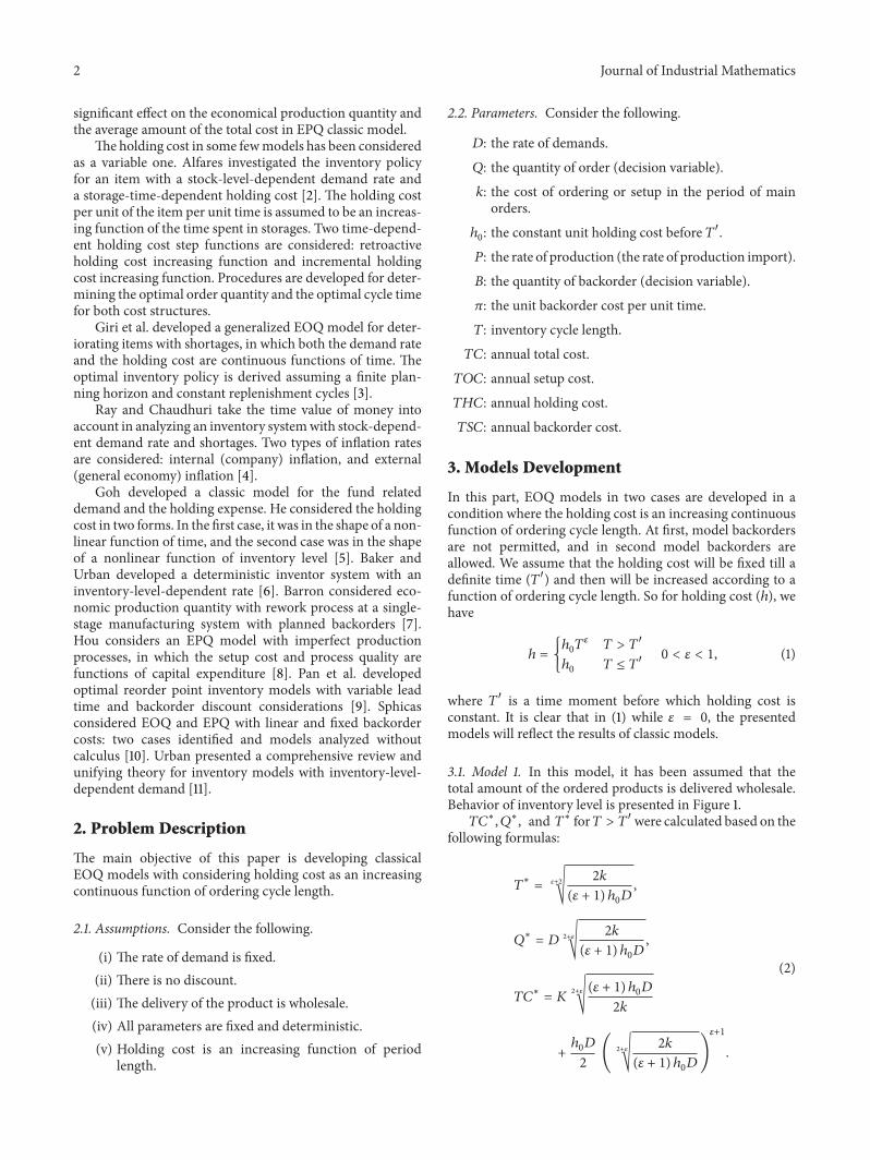
31 Model 1 In this model it has been assumed that thetotal amount of the ordered products is delivered wholesaleBehavior of inventory level is presented in Figure 1
119879119862lowast 119876lowast and 119879
lowast for119879 gt 1198791015840 were calculated based on the
following formulas
119879lowast=120576+2
radic2119896
(120576 + 1) ℎ0119863
119876lowast= 119863
2+120576
radic2119896
(120576 + 1) ℎ0119863
119879119862lowast= 119870
2+120576
radic(120576 + 1) ℎ0119863
2119896
+ℎ0119863
2(2+120576
radic2119896
(120576 + 1) ℎ0119863)
120576+1
(2)
Journal of Industrial Mathematics 3
I(t)
Q
Time
Figure 1 EOQ model without backorders
Proof The annual total cost is calculated based on the follow-ing procedures
119879119862 = 119879119874119862 + 119879119867119862 (3)
119879119862 =119863119896
119876+
ℎ119876
2 (4)
With replacing (1) in (4) we have
119879119862 =
119863119896
119876+
ℎ0119879120576119876
2119879 gt 119879
1015840
119863119896
119876+
ℎ0119876
2119879 le 119879
1015840
(5)
We know from classical inventory models that
119876 = 119863119879 (6)
So we can state that
119879119862 =
119896
119879+
ℎ0119905120576119863119879
2119879 gt 119879
1015840
119896
119879+
ℎ0119863119879
2119879 le 119879
1015840
(7)
For 119879 ge 1198791015840 we have
119879119862 =119896
119879+
ℎ0119863119879120576+1
2 (8)
By calculating first derivative of total cost function 119879119862
with respect to 119879 we have
119889119879119862
119889119879= minus
119896
1198792
+(120576 + 1) ℎ
0119863119879120576
2 (9)
Finally we can find the optimal period length as follows
minus119896
1198792+
(120576 + 1) ℎ0119863119879120576
2= 0
119896
1198792=
(120576 + 1) ℎ0119863119879120576
2
119879120576+2
=2119896
(120576 + 1) ℎ0119863
997904rArr 119879lowast=120576+2
radic2119896
(120576 + 1) ℎ0119863
(10)
Table 1 Optimal solution for different values of 120576 when backorderis not allowed
120576 119879lowast
119876lowast
119879119862lowast Loss ()
0 03536 84853 169706 001 03550 85204 161320 494372802 03577 85847 153760 939838503 03613 86701 146920 134287904 03654 87708 140730 170761905 03701 88826 135100 203936106 03751 90025 129960 234223107 03803 91281 125280 261799508 03857 92579 120980 287136909 03913 93903 117030 31041191 03969 95244 113390 3318602
The second derivative of 119879119862 with respect to 119879 is
1198892119879119862
1198891198792
=2119896
1198793+
120576 (120576 + 1) ℎ0119863119879120576minus1
2 (11)
As 0 lt 120576 lt 1 the previous equation is always positive sothat function 119879119862 is a convex function and 119879
lowast will be theminimum of function 119879119862 by replacing 119879
lowastin (6) the 119876lowast canbe calculated as follows
119876lowast= 119863 119879
lowast= 119863
2+120576
radic2119896
(120576 + 1) ℎ0119863
(12)
Then by replacing 119879lowastin (8) we get
119879119862lowast=
119896
2+120576
radic2119896 (120576 + 1) ℎ0119863
+ℎ0119863
2(2+120576
radic2119896
(120576 + 1) ℎ0119863)
120576+1
= 1198702+120576
radic(120576 + 1) ℎ0119863
2119896
+ℎ0119863
2(2+120576
radic2119896
(120576 + 1) ℎ0119863)
120576+1
(13)
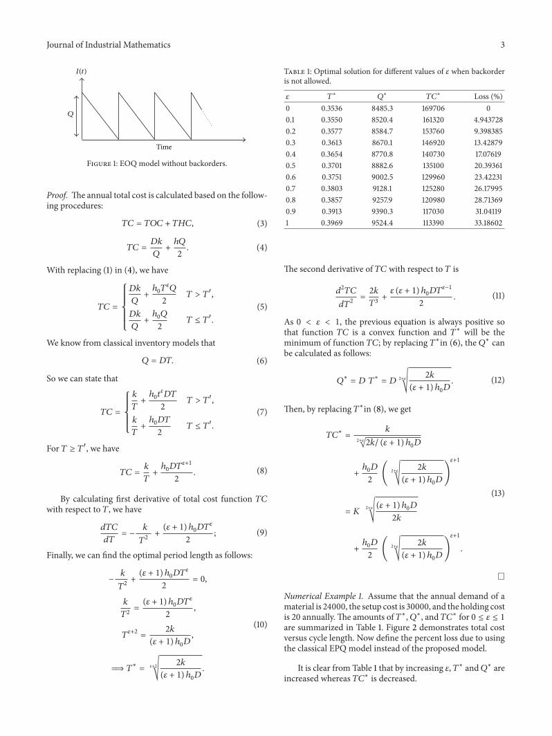
Numerical Example 1 Assume that the annual demand of amaterial is 24000 the setup cost is 30000 and the holding costis 20 annuallyThe amounts of 119879lowast119876lowast and 119879119862
lowast for 0 le 120576 le 1
are summarized in Table 1 Figure 2 demonstrates total costversus cycle length Now define the percent loss due to usingthe classical EPQ model instead of the proposed model
It is clear from Table 1 that by increasing 120576 119879lowast and119876lowast are
increased whereas 119879119862lowast is decreased
4 Journal of Industrial Mathematics
0 1
TC
2 3 4 50
2
4
6
8
T
106
Figure 2 Total cost versus cycle length for 120576 = 01 (Example 1)
32 Model 2 In this model we assume that the total amountof the ordered materials will be delivered to the store in awholesale where shortage is allowed Behavior of inventorylevel is presented in Figure 3 119905
2is the section of cycle for
which we have shortageIn this case the optimum amounts of 119879lowast 119876lowast and 119861
lowast for119879 gt 119879
1015840 are calculated based on the following formulas
119861lowast=
ℎ0119863 119879120576+1
ℎ0119879120576 + 120587
120587ℎ2
011986321198792120576+2
+ (120576 + 1) 1205872ℎ01198632119879120576+2
minus 2119896119863ℎ2
01198792120576
minus 4119896120587119863ℎ0119879120576minus 21205872119896119863 = 0
(14)
Proof See the appendix
Also we can calculate 119879119862lowast by replacing 119879lowast and 119861
lowast in
119879119862 (119879 119861) =119896
119879+
ℎ0119863119879120576+1
2minus ℎ0119861119879120576
+ℎ01198612119879120576minus1
2119863+
1205871198612
2119863119879
(15)
Proof of the convexity of 119879119862 and calculation of optimalsolution is mentioned in the appendix The overall convexityof total cost is not guaranteed but in special cases convexitycan be approved These cases are considered in the appendixtoo
Numerical Example 2 Assume that the annual need for a pro-duct is 24000 the setup cost is 95000 The holding cost is 50annually and the backorder cost for each product equals 250
t
Q
q
t1 t2
t
Net stock
minusb
Q minus b
Figure 3 EOQ model with backorders
Table 2 Optimal solutions for different values of 120576 when backorderis allowed
120576 119879lowast
119861lowast
119876lowast
119879119862lowast Loss ()
0 04359 17436 10461 435890 001 04335 16166 10404 421225 336438102 04324 15010 10377 407360 654522903 04322 13960 10373 394300 954139805 04343 12138 10423 370470 150083706 04362 11350 10470 359640 174929507 04387 10633 10528 349470 19826108 04415 99809 10596 339930 220147309 04447 93867 10672 330980 240681 04481 88454 10754 322570 2599738
Optimal values of 119879lowast 119879lowast119901 119876lowast and 119879119862
lowast for 0 le 120576 le 1 aresummarized in Table 2
It is clear fromTable 2 that by increasing 120576 119879lowast and119876
lowast areincreased and 119879119862
lowast is decreased Figure 4 demonstrates totalcost versus cycle length and amount of backorder
4 Conclusions and Suggestions
In this paper the classical EOQmodels have been developedby the consideration of holding cost as an increasing continu-ous function of ordering cycle length It was assumed that theholding cost will be fixed till a definite time and then will beincreased as a function of ordering cycle length Two modelswere developedThe first case does not allow backorders andother one permits backorders Economic ordering quantitythe optimum cycle length and the optimum total cost weredetermined in both cases From the numerical results wecould clearly see that loss due to using the classical EOQmodel is significant It is suggested for the future research thatthe holding cost be considered as different functions of theordering cycle length depend on reality
Journal of Industrial Mathematics 5
15
1007550
10050
250
T
104
108
TC(T B)
B
Figure 4 Result of Numerical Example 2 for 120576 = 01
Appendix
The annual total cost can be proved as follows
119879119862 (119879 119861) = 119879119874119862 + 119879119867119862 + 119879119878119862 (A1)
119879119862 (119879 119861) =119863119896
119876+
ℎ (119876 minus 119861)2
2119876+
1205871198612
2119876 (A2)
With replacing ℎ from (1) in (A2) we have
119879119862 (119879 119861) =
119863119896
119876+
ℎ0119879120576(119876 minus 119861)
2
2119876+
1205871198612
2119876 119879 gt 119879
1015840
119863119896
119876+
ℎ0(119876 minus 119861)
2
2119876+
1205871198612
2119876 119879 le 119879
1015840
(A3)
With replacing 119876 from (6) in (A3) we have
119879119862 (119879 119861)
=
119896
119879+
ℎ0119879120576(119863119879 minus 119861)
2
2119863119879+
1205871198612
2119863119879119879 gt 119879
1015840
119896
119879+
ℎ(119863119879 minus 119861)2
2119863119879+
1205871198612
2119863119879119879 le 119879
1015840
119879119862 (119879 119861)
=119896
119879+
ℎ0119879120576(11986321198792minus 2119863119879119861 + 119861
2)
2119863119879+
1205871198612
2119863119879
=119896
119879+
ℎ01198632119879120576+2
minus 2ℎ0119863119861119879120576+1
+ ℎ01198612119879120576
2119863119879+
1205871198612
2119863119879
=119896
119879+
ℎ0119863119879120576+1
2minus ℎ0119861119879120576+
ℎ01198612119879120576minus1
2119863+
1205871198612
2119863119879
(A4)
When 119879 gt 1198791015840 the gradient of 119879119862(119879 119861) function is in the
following form
nabla119879119862 (119879 119861) = (120597119862 (119879 119861)
120597119879120597119862 (119879 119861)
120597119861)
= (minus119896
1198792+
ℎ0119863(120576 + 1) 119879
120576
2minus ℎ0120576 119861 119879
120576minus1
+ℎ0 (120576 + 1) 119861
2119879120576minus2
2119863minus
1205871198612
21198631198792
minusℎ0119879120576+
ℎ0119879120576minus1
119863119861 +
120587119861
119863119879)
(A5)
The Hessian matrix of 119879119862(119879 119861) function can be calcu-lated as follows
119867 =
[[[[
[
1205972119879119862 (119879 119861)
1205971198792
1205972119879119862 (119879 119861)
120597119861120597119879
1205972119879119862 (119879 119861)
120597119879120597119861
1205972119879119862 (119879 119861)
1205971198612
]]]]
]
1205972119879119862 (119879 119861)
1205971198792
=2119870
1198793+
ℎ0119863120576 (120576 + 1) 119879
120576minus1
2minus ℎ0120576 (120576 minus 1) 119861119879
120576minus2
+ℎ0(120576 minus 1) (120576 minus 2) 119861
2119879120576minus3
2119863+
1205871198612
1198631198793
1205972119879119862 (119879 119861)
1205971198612
=ℎ0119879120576minus1
119863+
120587
119863119879
1205972119879119862 (119879 119861)
120597119879120597119861= minusℎ0120576119879120576minus1
+ℎ0 (120576 minus 1) 119861119879
120576minus2
119863minus
120587119861
1198631198792
1205972119879119862 (119879 119861)
120597119861120597119879= minusℎ0120576119879120576minus1
+ℎ0(120576 minus 1) 119861119879
120576minus2
119863minus
120587119861
1198631198792
(A6)
Since 0 lt 120576 lt 1 then 1205752119879119862(119879 119861)120575119879
2gt 0 is always true
The determinant of the119867matrix is computed as follows
|119867| = (1205972119879119862 (119879 119861)
1205971198792
)(1205972119879119862 (119879 119861)
1205971198612
)
minus (1205972119879119862 (119879 119861)
120597119861120597119879)
2
6 Journal of Industrial Mathematics
=2119896ℎ0119879120576minus4
119863+
ℎ2
0120576 (120576 + 1) 119879
2120576minus2
2
minusℎ2
0120576 (120576 minus 1) 119861119879
2120576minus3
119863
+ℎ2
0(120576 minus 1) (120576 minus 2) 119861
21198792120576minus4
21198632
+ℎ01205871198612119879120576minus4
1198632+
2120587119896
1198631198794+
120587ℎ0120576 (120576 + 1) 119879
120576minus2
2
minus120587ℎ0120576 (120576 minus 1) 119861119879
120576minus3
119863
+120587ℎ0(120576 minus 1) (120576 minus 2) 119861
2119879120576minus4
21198632
+12058721198612
11986321198794minus ℎ2
012057621198792120576minus2
+ℎ2
0120576 (120576 minus 1) 119861119879
2120576minus3
119863
minus120587ℎ0120576119861119879120576minus3
119863+
ℎ2
0120576 (120576 minus 1) 119861119879
2120576minus3
119863
minusℎ2
0(120576 minus 1)
211986121198792120576minus4
119863+
120587ℎ0(120576 minus 1) 119861
2119879120576minus4
1198632
minus120587ℎ0120576119861 119879120576minus3
119863+
120587ℎ0(120576 minus 1) 119861
2119879120576minus4
1198632
minus12058721198612
11986321198794
=2119870ℎ0119879120576minus4
119863+
ℎ2
0120576 (120576 minus 1) 119879
2120576minus2
2
+ℎ2
0(120576 minus 1) (120576 minus 2) 119861
21198792120576minus4
21198632
+ℎ01205871198612119879120576minus4
1198632
+2120587119870
1198631198794+
120587ℎ0120576 (120576 + 1) 119879
120576minus2
2
minus120587ℎ0120576 (120576 minus 1) 119861119879
120576minus3
119863
+120587ℎ0(120576 minus 1) (120576 minus 2) 119861
2119879120576minus4
21198632
minus ℎ2
012057621198792120576minus2
minus2120587ℎ0120576119861119879120576minus3
119863+
ℎ2
0120576 (120576 minus 1) 119861119879
120576minus3
119863
minusℎ2
0(120576 minus 1)
211986121198792120576minus4
1198632
+2120587ℎ0(120576 minus 1) 119861
2119879120576minus4
1198632
(A7)
Verifying the sign of mentioned relation (A7) seems impos-sible as while 120576 = 1 we have
|119867| =2119896ℎ0119879minus3
119863+ ℎ2
0+
ℎ01205871198612119879minus3
1198632+
2120587119896
1198631198794
+ 120587ℎ0119879minus1
minus ℎ2
0minus
2120587ℎ0119861119879minus2
119863
=2119896ℎ0
1198631198793+
ℎ01205871198612
11986321198793+
2120587119896
1198631198794+
120587ℎ0
119879minus
2120587ℎ0119861
1198631198792
= (4119896ℎ0119863119879 + 2ℎ
01205871198612119879 + 4120587119896119863 + 2120587ℎ
011986321198793
minus4120587ℎ01198611198631198792) (2119863
21198794)minus1
(A8)
While 120576 = 1 if one of the following conditions (A9) isrealized the determinant of 119867 would not be negative and119879119862(119879 119861)will be convex It should bementioned that this con-dition is not the most essential condition but is an adequatecondition Consider
2119896ℎ0119863119879 + ℎ
01205871198612119879 + 2120587119896119863 + 120587ℎ
011986321198793
minus 2120587ℎ0119861119863 119879
2gt 0
2119896ℎ0119863119879 gt 2120587ℎ
01198611198631198792997904rArr 119861 gt 2119863119879
ℎ01205871198612119879 gt 2120587ℎ
01198611198631198792997904rArr 119896 gt 120587119861119879
2120587119896119863 gt 2120587ℎ01198611198631198792997904rArr 119896 gt ℎ
01198611198792
120587ℎ011986321198793gt 2120587ℎ
01198611198631198792997904rArr 2119863119879 gt 119861
(A9)
For finding minimum points of 119879119862 we survey its conditionas follows
119879119862 is positive 119879119862 is always continuous for 119879 gt 0 and119861 gt 0 Also there is a section for which function119879119862 is convex(when 119879 rarr 0
+ 119879119862 rarr +infin)
The gradient vector is always available when 119879 is positive(1205972119879119862(119879 119861)120597119879
2) is always positive so the 119879119862 is not concave
and the extremumpoints will be in types ofminimumpointsConsider the following
119879119862 does not have a local maximum point or a totalmaximum point When 119879 rarr 0
+ then 119879119862 rarr +infin when119861 rarr 0
+ then 119879119862 rarr +infin when 119879 rarr +infin then 119879119862 rarr
+infinSo these cases provide just the following two conditions
for function 119879119862(119879 119861)
(i) Function 119879119862(119879 119861) has a local minimum point thatcan be considered as an optimal point which isobtained from solving (A10) In this case (A10) hasonly one real root
(ii) Function 119879119862(119879 119861) has some local minimum pointsand some saddle points such that the maximumnumber of these points is lceil2120576 + 2rceil One of thesepoints will be the optimal minimum point and theother points will be the local minimum or saddlepoints Based on the aforementioned conditions the119879119862(119879 119861) function will certainly have an optimalminimum point In this case (A10) will have morethan one real root If the determinant of Hessianmatrix is positive then the point will be minimumand if the determinant of Hessian matrix is negativethen the point will be saddle The optimal solution isone of minimum points which has the lowest amountof 119879119862
Journal of Industrial Mathematics 7
For finding the optimal solution we have
nabla119879119862 (119879 119861) = 0 (A10)
(120597119879119862 (119879 119861)
120597119879120597119879119862 (119879 119861)
120597119861) = 0 (A11)
(minus119896
1198792+
ℎ0119863 (120576 + 1) 119879
120576
2minus ℎ0120576119861119879120576minus1
+ℎ0(120576 + 1) 119861
2119879120576minus2
2119863
minus1205871198612
21198631198792 minusℎ0119879120576+
ℎ0119879120576minus1
119863119861 +
120587119861
119863119879) = 0
(A12)
minus119896
1198792+
ℎ0119863 (120576 + 1) 119879
120576
2minus ℎ0120576119861119879120576minus1
+ℎ0(120576 + 1) 119861
2119879120576minus2
2119863minus
1205871198612
21198631198792= 0
(A13)
minusℎ0119879120576+
ℎ0119879120576minus1
119863119861 +
120587119861
119863119879= 0 (A14)
997904rArr 119861 =ℎ0119863119879120576+1
ℎ0119879120576 + 120587
(A15)
With replacing (A15) in (A14) we have
120587ℎ2
011986321198792120576+2
+ (120576 + 1) 1205872ℎ01198632119879120576+2
minus 2119896119863ℎ2
01198792120576
minus 4119896120587119863ℎ0119879120576minus 21205872119896119863 = 0
(A16)
Finally we can obtain optimal solution for 119879 by solving(A16)
References
[1] M A Darwish ldquoEPQmodels with varying setup costrdquo Interna-tional Journal of Production Economics vol 113 no 1 pp 297ndash306 2008
[2] H K Alfares ldquoInventory model with stock-level dependentdemand rate and variable holding costrdquo International Journalof Production Economics vol 108 no 1-2 pp 259ndash265 2007
[3] B C Giri A Goswami and K S Chaudhuri ldquoAn EOQ modelfor deteriorating items with time varying demand and costsrdquoJournal of the Operational Research Society vol 47 no 11 pp1398ndash1405 1996
[4] J Ray and K S Chaudhuri ldquoAn EOQ model with stock-dependent demand shortage inflation and time discountingrdquoInternational Journal of Production Economics vol 53 no 2 pp171ndash180 1997
[5] M Goh ldquoSome results for inventory models having inventorylevel dependent demand raterdquo International Journal of Produc-tion Economics vol 27 no 2 pp 155ndash160 1992
[6] R C Baker and T L Urban ldquoA deterministic inventor systemwith an inventory level dependent raterdquo Journal of the OperationResearch Society vol 39 no 9 pp 823ndash831 1988
[7] L E C Barron ldquoEconomic production quantity with reworkprocess at a single-stage manufacturing system with plannedbackordersrdquo Computers and Industrial Engineering vol 57 no3 pp 1105ndash1113 2009
[8] K L Hou ldquoAn EPQ model with setup cost and process qualityas functions of capital expenditurerdquo Applied MathematicalModelling vol 31 no 1 pp 10ndash17 2007
[9] J C H Pan M C Lo and Y C Hsiao ldquoOptimal reorderpoint inventory models with variable lead time and backo-rder discount considerationsrdquo European Journal of OperationalResearch vol 158 no 2 pp 488ndash505 2004
[10] G P Sphicas ldquoEOQ and EPQ with linear and fixed backordercosts two cases identified and models analyzed without calcu-lusrdquo International Journal of Production Economics vol 100 no1 pp 59ndash64 2006
[11] T L Urban ldquoInventorymodels with inventory-level-dependentdemand a comprehensive review and unifying theoryrdquo Euro-pean Journal of Operational Research vol 162 no 3 pp 792ndash804 2005
Submit your manuscripts athttpwwwhindawicom
Hindawi Publishing Corporationhttpwwwhindawicom Volume 2014
MathematicsJournal of
Hindawi Publishing Corporationhttpwwwhindawicom Volume 2014
Mathematical Problems in Engineering
Hindawi Publishing Corporationhttpwwwhindawicom
Differential EquationsInternational Journal of
Volume 2014
Applied MathematicsJournal of
Hindawi Publishing Corporationhttpwwwhindawicom Volume 2014
Probability and StatisticsHindawi Publishing Corporationhttpwwwhindawicom Volume 2014
Journal of
Hindawi Publishing Corporationhttpwwwhindawicom Volume 2014
Mathematical PhysicsAdvances in
Complex AnalysisJournal of
Hindawi Publishing Corporationhttpwwwhindawicom Volume 2014
OptimizationJournal of
Hindawi Publishing Corporationhttpwwwhindawicom Volume 2014
CombinatoricsHindawi Publishing Corporationhttpwwwhindawicom Volume 2014
International Journal of
Hindawi Publishing Corporationhttpwwwhindawicom Volume 2014
Operations ResearchAdvances in
Journal of
Hindawi Publishing Corporationhttpwwwhindawicom Volume 2014
Function Spaces
Abstract and Applied AnalysisHindawi Publishing Corporationhttpwwwhindawicom Volume 2014
International Journal of Mathematics and Mathematical Sciences
Hindawi Publishing Corporationhttpwwwhindawicom Volume 2014
The Scientific World JournalHindawi Publishing Corporation httpwwwhindawicom Volume 2014
Hindawi Publishing Corporationhttpwwwhindawicom Volume 2014
Algebra
Discrete Dynamics in Nature and Society
Hindawi Publishing Corporationhttpwwwhindawicom Volume 2014
Hindawi Publishing Corporationhttpwwwhindawicom Volume 2014
Decision SciencesAdvances in
Discrete MathematicsJournal of
Hindawi Publishing Corporationhttpwwwhindawicom
Volume 2014 Hindawi Publishing Corporationhttpwwwhindawicom Volume 2014
Stochastic AnalysisInternational Journal of
2 Journal of Industrial Mathematics
significant effect on the economical production quantity andthe average amount of the total cost in EPQ classic model
The holding cost in some fewmodels has been consideredas a variable one Alfares investigated the inventory policyfor an item with a stock-level-dependent demand rate anda storage-time-dependent holding cost [2] The holding costper unit of the item per unit time is assumed to be an increas-ing function of the time spent in storages Two time-depend-ent holding cost step functions are considered retroactiveholding cost increasing function and incremental holdingcost increasing function Procedures are developed for deter-mining the optimal order quantity and the optimal cycle timefor both cost structures
Giri et al developed a generalized EOQ model for deter-iorating items with shortages in which both the demand rateand the holding cost are continuous functions of time Theoptimal inventory policy is derived assuming a finite plan-ning horizon and constant replenishment cycles [3]
Ray and Chaudhuri take the time value of money intoaccount in analyzing an inventory systemwith stock-depend-ent demand rate and shortages Two types of inflation ratesare considered internal (company) inflation and external(general economy) inflation [4]
Goh developed a classic model for the fund relateddemand and the holding expense He considered the holdingcost in two forms In the first case it was in the shape of a non-linear function of time and the second case was in the shapeof a nonlinear function of inventory level [5] Baker andUrban developed a deterministic inventor system with aninventory-level-dependent rate [6] Barron considered eco-nomic production quantity with rework process at a single-stage manufacturing system with planned backorders [7]Hou considers an EPQ model with imperfect productionprocesses in which the setup cost and process quality arefunctions of capital expenditure [8] Pan et al developedoptimal reorder point inventory models with variable leadtime and backorder discount considerations [9] Sphicasconsidered EOQ and EPQ with linear and fixed backordercosts two cases identified and models analyzed withoutcalculus [10] Urban presented a comprehensive review andunifying theory for inventory models with inventory-level-dependent demand [11]
2 Problem Description
The main objective of this paper is developing classicalEOQ models with considering holding cost as an increasingcontinuous function of ordering cycle length
21 Assumptions Consider the following
(i) The rate of demand is fixed(ii) There is no discount(iii) The delivery of the product is wholesale(iv) All parameters are fixed and deterministic(v) Holding cost is an increasing function of period
length
22 Parameters Consider the following
119863 the rate of demands119876 the quantity of order (decision variable)119896 the cost of ordering or setup in the period of main
ordersℎ0 the constant unit holding cost before 1198791015840
119875 the rate of production (the rate of production import)119861 the quantity of backorder (decision variable)120587 the unit backorder cost per unit time119879 inventory cycle length
119879119862 annual total cost119879119874119862 annual setup cost119879119867119862 annual holding cost119879119878119862 annual backorder cost
3 Models Development
In this part EOQ models in two cases are developed in acondition where the holding cost is an increasing continuousfunction of ordering cycle length At first model backordersare not permitted and in second model backorders areallowed We assume that the holding cost will be fixed till adefinite time (1198791015840) and then will be increased according to afunction of ordering cycle length So for holding cost (ℎ) wehave
ℎ = ℎ0119879120576
119879 gt 1198791015840
ℎ0
119879 le 1198791015840
0 lt 120576 lt 1 (1)
where 1198791015840 is a time moment before which holding cost is
constant It is clear that in (1) while 120576 = 0 the presentedmodels will reflect the results of classic models
31 Model 1 In this model it has been assumed that thetotal amount of the ordered products is delivered wholesaleBehavior of inventory level is presented in Figure 1
119879119862lowast 119876lowast and 119879
lowast for119879 gt 1198791015840 were calculated based on the
following formulas
119879lowast=120576+2
radic2119896
(120576 + 1) ℎ0119863
119876lowast= 119863
2+120576
radic2119896
(120576 + 1) ℎ0119863
119879119862lowast= 119870
2+120576
radic(120576 + 1) ℎ0119863
2119896
+ℎ0119863
2(2+120576
radic2119896
(120576 + 1) ℎ0119863)
120576+1
(2)
Journal of Industrial Mathematics 3
I(t)
Q
Time
Figure 1 EOQ model without backorders
Proof The annual total cost is calculated based on the follow-ing procedures
119879119862 = 119879119874119862 + 119879119867119862 (3)
119879119862 =119863119896
119876+
ℎ119876
2 (4)
With replacing (1) in (4) we have
119879119862 =
119863119896
119876+
ℎ0119879120576119876
2119879 gt 119879
1015840
119863119896
119876+
ℎ0119876
2119879 le 119879
1015840
(5)
We know from classical inventory models that
119876 = 119863119879 (6)
So we can state that
119879119862 =
119896
119879+
ℎ0119905120576119863119879
2119879 gt 119879
1015840
119896
119879+
ℎ0119863119879
2119879 le 119879
1015840
(7)
For 119879 ge 1198791015840 we have
119879119862 =119896
119879+
ℎ0119863119879120576+1
2 (8)
By calculating first derivative of total cost function 119879119862
with respect to 119879 we have
119889119879119862
119889119879= minus
119896
1198792
+(120576 + 1) ℎ
0119863119879120576
2 (9)
Finally we can find the optimal period length as follows
minus119896
1198792+
(120576 + 1) ℎ0119863119879120576
2= 0
119896
1198792=
(120576 + 1) ℎ0119863119879120576
2
119879120576+2
=2119896
(120576 + 1) ℎ0119863
997904rArr 119879lowast=120576+2
radic2119896
(120576 + 1) ℎ0119863
(10)
Table 1 Optimal solution for different values of 120576 when backorderis not allowed
120576 119879lowast
119876lowast
119879119862lowast Loss ()
0 03536 84853 169706 001 03550 85204 161320 494372802 03577 85847 153760 939838503 03613 86701 146920 134287904 03654 87708 140730 170761905 03701 88826 135100 203936106 03751 90025 129960 234223107 03803 91281 125280 261799508 03857 92579 120980 287136909 03913 93903 117030 31041191 03969 95244 113390 3318602
The second derivative of 119879119862 with respect to 119879 is
1198892119879119862
1198891198792
=2119896
1198793+
120576 (120576 + 1) ℎ0119863119879120576minus1
2 (11)
As 0 lt 120576 lt 1 the previous equation is always positive sothat function 119879119862 is a convex function and 119879
lowast will be theminimum of function 119879119862 by replacing 119879
lowastin (6) the 119876lowast canbe calculated as follows
119876lowast= 119863 119879
lowast= 119863
2+120576
radic2119896
(120576 + 1) ℎ0119863
(12)
Then by replacing 119879lowastin (8) we get
119879119862lowast=
119896
2+120576
radic2119896 (120576 + 1) ℎ0119863
+ℎ0119863
2(2+120576
radic2119896
(120576 + 1) ℎ0119863)
120576+1
= 1198702+120576
radic(120576 + 1) ℎ0119863
2119896
+ℎ0119863
2(2+120576
radic2119896
(120576 + 1) ℎ0119863)
120576+1
(13)
Numerical Example 1 Assume that the annual demand of amaterial is 24000 the setup cost is 30000 and the holding costis 20 annuallyThe amounts of 119879lowast119876lowast and 119879119862
lowast for 0 le 120576 le 1
are summarized in Table 1 Figure 2 demonstrates total costversus cycle length Now define the percent loss due to usingthe classical EPQ model instead of the proposed model
It is clear from Table 1 that by increasing 120576 119879lowast and119876lowast are
increased whereas 119879119862lowast is decreased
4 Journal of Industrial Mathematics
0 1
TC
2 3 4 50
2
4
6
8
T
106
Figure 2 Total cost versus cycle length for 120576 = 01 (Example 1)
32 Model 2 In this model we assume that the total amountof the ordered materials will be delivered to the store in awholesale where shortage is allowed Behavior of inventorylevel is presented in Figure 3 119905
2is the section of cycle for
which we have shortageIn this case the optimum amounts of 119879lowast 119876lowast and 119861
lowast for119879 gt 119879
1015840 are calculated based on the following formulas
119861lowast=
ℎ0119863 119879120576+1
ℎ0119879120576 + 120587
120587ℎ2
011986321198792120576+2
+ (120576 + 1) 1205872ℎ01198632119879120576+2
minus 2119896119863ℎ2
01198792120576
minus 4119896120587119863ℎ0119879120576minus 21205872119896119863 = 0
(14)
Proof See the appendix
Also we can calculate 119879119862lowast by replacing 119879lowast and 119861
lowast in
119879119862 (119879 119861) =119896
119879+
ℎ0119863119879120576+1
2minus ℎ0119861119879120576
+ℎ01198612119879120576minus1
2119863+
1205871198612
2119863119879
(15)
Proof of the convexity of 119879119862 and calculation of optimalsolution is mentioned in the appendix The overall convexityof total cost is not guaranteed but in special cases convexitycan be approved These cases are considered in the appendixtoo
Numerical Example 2 Assume that the annual need for a pro-duct is 24000 the setup cost is 95000 The holding cost is 50annually and the backorder cost for each product equals 250
t
Q
q
t1 t2
t
Net stock
minusb
Q minus b
Figure 3 EOQ model with backorders
Table 2 Optimal solutions for different values of 120576 when backorderis allowed
120576 119879lowast
119861lowast
119876lowast
119879119862lowast Loss ()
0 04359 17436 10461 435890 001 04335 16166 10404 421225 336438102 04324 15010 10377 407360 654522903 04322 13960 10373 394300 954139805 04343 12138 10423 370470 150083706 04362 11350 10470 359640 174929507 04387 10633 10528 349470 19826108 04415 99809 10596 339930 220147309 04447 93867 10672 330980 240681 04481 88454 10754 322570 2599738
Optimal values of 119879lowast 119879lowast119901 119876lowast and 119879119862
lowast for 0 le 120576 le 1 aresummarized in Table 2
It is clear fromTable 2 that by increasing 120576 119879lowast and119876
lowast areincreased and 119879119862
lowast is decreased Figure 4 demonstrates totalcost versus cycle length and amount of backorder
4 Conclusions and Suggestions
In this paper the classical EOQmodels have been developedby the consideration of holding cost as an increasing continu-ous function of ordering cycle length It was assumed that theholding cost will be fixed till a definite time and then will beincreased as a function of ordering cycle length Two modelswere developedThe first case does not allow backorders andother one permits backorders Economic ordering quantitythe optimum cycle length and the optimum total cost weredetermined in both cases From the numerical results wecould clearly see that loss due to using the classical EOQmodel is significant It is suggested for the future research thatthe holding cost be considered as different functions of theordering cycle length depend on reality
Journal of Industrial Mathematics 5
15
1007550
10050
250
T
104
108
TC(T B)
B
Figure 4 Result of Numerical Example 2 for 120576 = 01
Appendix
The annual total cost can be proved as follows
119879119862 (119879 119861) = 119879119874119862 + 119879119867119862 + 119879119878119862 (A1)
119879119862 (119879 119861) =119863119896
119876+
ℎ (119876 minus 119861)2
2119876+
1205871198612
2119876 (A2)
With replacing ℎ from (1) in (A2) we have
119879119862 (119879 119861) =
119863119896
119876+
ℎ0119879120576(119876 minus 119861)
2
2119876+
1205871198612
2119876 119879 gt 119879
1015840
119863119896
119876+
ℎ0(119876 minus 119861)
2
2119876+
1205871198612
2119876 119879 le 119879
1015840
(A3)
With replacing 119876 from (6) in (A3) we have
119879119862 (119879 119861)
=
119896
119879+
ℎ0119879120576(119863119879 minus 119861)
2
2119863119879+
1205871198612
2119863119879119879 gt 119879
1015840
119896
119879+
ℎ(119863119879 minus 119861)2
2119863119879+
1205871198612
2119863119879119879 le 119879
1015840
119879119862 (119879 119861)
=119896
119879+
ℎ0119879120576(11986321198792minus 2119863119879119861 + 119861
2)
2119863119879+
1205871198612
2119863119879
=119896
119879+
ℎ01198632119879120576+2
minus 2ℎ0119863119861119879120576+1
+ ℎ01198612119879120576
2119863119879+
1205871198612
2119863119879
=119896
119879+
ℎ0119863119879120576+1
2minus ℎ0119861119879120576+
ℎ01198612119879120576minus1
2119863+
1205871198612
2119863119879
(A4)
When 119879 gt 1198791015840 the gradient of 119879119862(119879 119861) function is in the
following form
nabla119879119862 (119879 119861) = (120597119862 (119879 119861)
120597119879120597119862 (119879 119861)
120597119861)
= (minus119896
1198792+
ℎ0119863(120576 + 1) 119879
120576
2minus ℎ0120576 119861 119879
120576minus1
+ℎ0 (120576 + 1) 119861
2119879120576minus2
2119863minus
1205871198612
21198631198792
minusℎ0119879120576+
ℎ0119879120576minus1
119863119861 +
120587119861
119863119879)
(A5)
The Hessian matrix of 119879119862(119879 119861) function can be calcu-lated as follows
119867 =
[[[[
[
1205972119879119862 (119879 119861)
1205971198792
1205972119879119862 (119879 119861)
120597119861120597119879
1205972119879119862 (119879 119861)
120597119879120597119861
1205972119879119862 (119879 119861)
1205971198612
]]]]
]
1205972119879119862 (119879 119861)
1205971198792
=2119870
1198793+
ℎ0119863120576 (120576 + 1) 119879
120576minus1
2minus ℎ0120576 (120576 minus 1) 119861119879
120576minus2
+ℎ0(120576 minus 1) (120576 minus 2) 119861
2119879120576minus3
2119863+
1205871198612
1198631198793
1205972119879119862 (119879 119861)
1205971198612
=ℎ0119879120576minus1
119863+
120587
119863119879
1205972119879119862 (119879 119861)
120597119879120597119861= minusℎ0120576119879120576minus1
+ℎ0 (120576 minus 1) 119861119879
120576minus2
119863minus
120587119861
1198631198792
1205972119879119862 (119879 119861)
120597119861120597119879= minusℎ0120576119879120576minus1
+ℎ0(120576 minus 1) 119861119879
120576minus2
119863minus
120587119861
1198631198792
(A6)
Since 0 lt 120576 lt 1 then 1205752119879119862(119879 119861)120575119879
2gt 0 is always true
The determinant of the119867matrix is computed as follows
|119867| = (1205972119879119862 (119879 119861)
1205971198792
)(1205972119879119862 (119879 119861)
1205971198612
)
minus (1205972119879119862 (119879 119861)
120597119861120597119879)
2
6 Journal of Industrial Mathematics
=2119896ℎ0119879120576minus4
119863+
ℎ2
0120576 (120576 + 1) 119879
2120576minus2
2
minusℎ2
0120576 (120576 minus 1) 119861119879
2120576minus3
119863
+ℎ2
0(120576 minus 1) (120576 minus 2) 119861
21198792120576minus4
21198632
+ℎ01205871198612119879120576minus4
1198632+
2120587119896
1198631198794+
120587ℎ0120576 (120576 + 1) 119879
120576minus2
2
minus120587ℎ0120576 (120576 minus 1) 119861119879
120576minus3
119863
+120587ℎ0(120576 minus 1) (120576 minus 2) 119861
2119879120576minus4
21198632
+12058721198612
11986321198794minus ℎ2
012057621198792120576minus2
+ℎ2
0120576 (120576 minus 1) 119861119879
2120576minus3
119863
minus120587ℎ0120576119861119879120576minus3
119863+
ℎ2
0120576 (120576 minus 1) 119861119879
2120576minus3
119863
minusℎ2
0(120576 minus 1)
211986121198792120576minus4
119863+
120587ℎ0(120576 minus 1) 119861
2119879120576minus4
1198632
minus120587ℎ0120576119861 119879120576minus3
119863+
120587ℎ0(120576 minus 1) 119861
2119879120576minus4
1198632
minus12058721198612
11986321198794
=2119870ℎ0119879120576minus4
119863+
ℎ2
0120576 (120576 minus 1) 119879
2120576minus2
2
+ℎ2
0(120576 minus 1) (120576 minus 2) 119861
21198792120576minus4
21198632
+ℎ01205871198612119879120576minus4
1198632
+2120587119870
1198631198794+
120587ℎ0120576 (120576 + 1) 119879
120576minus2
2
minus120587ℎ0120576 (120576 minus 1) 119861119879
120576minus3
119863
+120587ℎ0(120576 minus 1) (120576 minus 2) 119861
2119879120576minus4
21198632
minus ℎ2
012057621198792120576minus2
minus2120587ℎ0120576119861119879120576minus3
119863+
ℎ2
0120576 (120576 minus 1) 119861119879
120576minus3
119863
minusℎ2
0(120576 minus 1)
211986121198792120576minus4
1198632
+2120587ℎ0(120576 minus 1) 119861
2119879120576minus4
1198632
(A7)
Verifying the sign of mentioned relation (A7) seems impos-sible as while 120576 = 1 we have
|119867| =2119896ℎ0119879minus3
119863+ ℎ2
0+
ℎ01205871198612119879minus3
1198632+
2120587119896
1198631198794
+ 120587ℎ0119879minus1
minus ℎ2
0minus
2120587ℎ0119861119879minus2
119863
=2119896ℎ0
1198631198793+
ℎ01205871198612
11986321198793+
2120587119896
1198631198794+
120587ℎ0
119879minus
2120587ℎ0119861
1198631198792
= (4119896ℎ0119863119879 + 2ℎ
01205871198612119879 + 4120587119896119863 + 2120587ℎ
011986321198793
minus4120587ℎ01198611198631198792) (2119863
21198794)minus1
(A8)
While 120576 = 1 if one of the following conditions (A9) isrealized the determinant of 119867 would not be negative and119879119862(119879 119861)will be convex It should bementioned that this con-dition is not the most essential condition but is an adequatecondition Consider
2119896ℎ0119863119879 + ℎ
01205871198612119879 + 2120587119896119863 + 120587ℎ
011986321198793
minus 2120587ℎ0119861119863 119879
2gt 0
2119896ℎ0119863119879 gt 2120587ℎ
01198611198631198792997904rArr 119861 gt 2119863119879
ℎ01205871198612119879 gt 2120587ℎ
01198611198631198792997904rArr 119896 gt 120587119861119879
2120587119896119863 gt 2120587ℎ01198611198631198792997904rArr 119896 gt ℎ
01198611198792
120587ℎ011986321198793gt 2120587ℎ
01198611198631198792997904rArr 2119863119879 gt 119861
(A9)
For finding minimum points of 119879119862 we survey its conditionas follows
119879119862 is positive 119879119862 is always continuous for 119879 gt 0 and119861 gt 0 Also there is a section for which function119879119862 is convex(when 119879 rarr 0
+ 119879119862 rarr +infin)
The gradient vector is always available when 119879 is positive(1205972119879119862(119879 119861)120597119879
2) is always positive so the 119879119862 is not concave
and the extremumpoints will be in types ofminimumpointsConsider the following
119879119862 does not have a local maximum point or a totalmaximum point When 119879 rarr 0
+ then 119879119862 rarr +infin when119861 rarr 0
+ then 119879119862 rarr +infin when 119879 rarr +infin then 119879119862 rarr
+infinSo these cases provide just the following two conditions
for function 119879119862(119879 119861)
(i) Function 119879119862(119879 119861) has a local minimum point thatcan be considered as an optimal point which isobtained from solving (A10) In this case (A10) hasonly one real root
(ii) Function 119879119862(119879 119861) has some local minimum pointsand some saddle points such that the maximumnumber of these points is lceil2120576 + 2rceil One of thesepoints will be the optimal minimum point and theother points will be the local minimum or saddlepoints Based on the aforementioned conditions the119879119862(119879 119861) function will certainly have an optimalminimum point In this case (A10) will have morethan one real root If the determinant of Hessianmatrix is positive then the point will be minimumand if the determinant of Hessian matrix is negativethen the point will be saddle The optimal solution isone of minimum points which has the lowest amountof 119879119862
Journal of Industrial Mathematics 7
For finding the optimal solution we have
nabla119879119862 (119879 119861) = 0 (A10)
(120597119879119862 (119879 119861)
120597119879120597119879119862 (119879 119861)
120597119861) = 0 (A11)
(minus119896
1198792+
ℎ0119863 (120576 + 1) 119879
120576
2minus ℎ0120576119861119879120576minus1
+ℎ0(120576 + 1) 119861
2119879120576minus2
2119863
minus1205871198612
21198631198792 minusℎ0119879120576+
ℎ0119879120576minus1
119863119861 +
120587119861
119863119879) = 0
(A12)
minus119896
1198792+
ℎ0119863 (120576 + 1) 119879
120576
2minus ℎ0120576119861119879120576minus1
+ℎ0(120576 + 1) 119861
2119879120576minus2
2119863minus
1205871198612
21198631198792= 0
(A13)
minusℎ0119879120576+
ℎ0119879120576minus1
119863119861 +
120587119861
119863119879= 0 (A14)
997904rArr 119861 =ℎ0119863119879120576+1
ℎ0119879120576 + 120587
(A15)
With replacing (A15) in (A14) we have
120587ℎ2
011986321198792120576+2
+ (120576 + 1) 1205872ℎ01198632119879120576+2
minus 2119896119863ℎ2
01198792120576
minus 4119896120587119863ℎ0119879120576minus 21205872119896119863 = 0
(A16)
Finally we can obtain optimal solution for 119879 by solving(A16)
References
[1] M A Darwish ldquoEPQmodels with varying setup costrdquo Interna-tional Journal of Production Economics vol 113 no 1 pp 297ndash306 2008
[2] H K Alfares ldquoInventory model with stock-level dependentdemand rate and variable holding costrdquo International Journalof Production Economics vol 108 no 1-2 pp 259ndash265 2007
[3] B C Giri A Goswami and K S Chaudhuri ldquoAn EOQ modelfor deteriorating items with time varying demand and costsrdquoJournal of the Operational Research Society vol 47 no 11 pp1398ndash1405 1996
[4] J Ray and K S Chaudhuri ldquoAn EOQ model with stock-dependent demand shortage inflation and time discountingrdquoInternational Journal of Production Economics vol 53 no 2 pp171ndash180 1997
[5] M Goh ldquoSome results for inventory models having inventorylevel dependent demand raterdquo International Journal of Produc-tion Economics vol 27 no 2 pp 155ndash160 1992
[6] R C Baker and T L Urban ldquoA deterministic inventor systemwith an inventory level dependent raterdquo Journal of the OperationResearch Society vol 39 no 9 pp 823ndash831 1988
[7] L E C Barron ldquoEconomic production quantity with reworkprocess at a single-stage manufacturing system with plannedbackordersrdquo Computers and Industrial Engineering vol 57 no3 pp 1105ndash1113 2009
[8] K L Hou ldquoAn EPQ model with setup cost and process qualityas functions of capital expenditurerdquo Applied MathematicalModelling vol 31 no 1 pp 10ndash17 2007
[9] J C H Pan M C Lo and Y C Hsiao ldquoOptimal reorderpoint inventory models with variable lead time and backo-rder discount considerationsrdquo European Journal of OperationalResearch vol 158 no 2 pp 488ndash505 2004
[10] G P Sphicas ldquoEOQ and EPQ with linear and fixed backordercosts two cases identified and models analyzed without calcu-lusrdquo International Journal of Production Economics vol 100 no1 pp 59ndash64 2006
[11] T L Urban ldquoInventorymodels with inventory-level-dependentdemand a comprehensive review and unifying theoryrdquo Euro-pean Journal of Operational Research vol 162 no 3 pp 792ndash804 2005
Submit your manuscripts athttpwwwhindawicom
Hindawi Publishing Corporationhttpwwwhindawicom Volume 2014
MathematicsJournal of
Hindawi Publishing Corporationhttpwwwhindawicom Volume 2014
Mathematical Problems in Engineering
Hindawi Publishing Corporationhttpwwwhindawicom
Differential EquationsInternational Journal of
Volume 2014
Applied MathematicsJournal of
Hindawi Publishing Corporationhttpwwwhindawicom Volume 2014
Probability and StatisticsHindawi Publishing Corporationhttpwwwhindawicom Volume 2014
Journal of
Hindawi Publishing Corporationhttpwwwhindawicom Volume 2014
Mathematical PhysicsAdvances in
Complex AnalysisJournal of
Hindawi Publishing Corporationhttpwwwhindawicom Volume 2014
OptimizationJournal of
Hindawi Publishing Corporationhttpwwwhindawicom Volume 2014
CombinatoricsHindawi Publishing Corporationhttpwwwhindawicom Volume 2014
International Journal of
Hindawi Publishing Corporationhttpwwwhindawicom Volume 2014
Operations ResearchAdvances in
Journal of
Hindawi Publishing Corporationhttpwwwhindawicom Volume 2014
Function Spaces
Abstract and Applied AnalysisHindawi Publishing Corporationhttpwwwhindawicom Volume 2014
International Journal of Mathematics and Mathematical Sciences
Hindawi Publishing Corporationhttpwwwhindawicom Volume 2014
The Scientific World JournalHindawi Publishing Corporation httpwwwhindawicom Volume 2014
Hindawi Publishing Corporationhttpwwwhindawicom Volume 2014
Algebra
Discrete Dynamics in Nature and Society
Hindawi Publishing Corporationhttpwwwhindawicom Volume 2014
Hindawi Publishing Corporationhttpwwwhindawicom Volume 2014
Decision SciencesAdvances in
Discrete MathematicsJournal of
Hindawi Publishing Corporationhttpwwwhindawicom
Volume 2014 Hindawi Publishing Corporationhttpwwwhindawicom Volume 2014
Stochastic AnalysisInternational Journal of
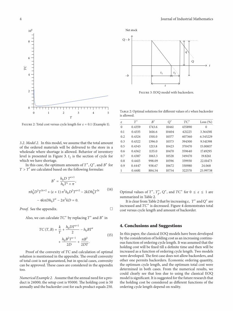
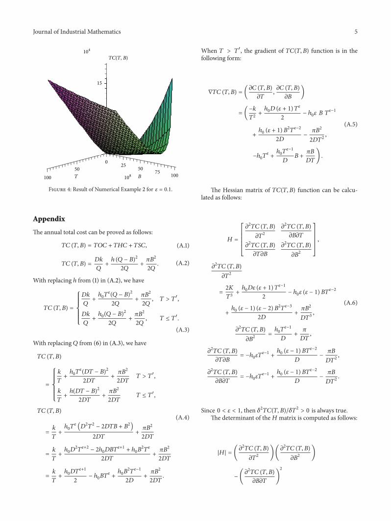