resolving turbulence- chemistry interactions in mixing ... · resolving turbulence-chemistry...

RESOLVING TURBULENCE- CHEMISTRY INTERACTIONS IN MIXING-CONTROLLED COMBUSTION WITH LES AND DETAILED CHEMISTRYConvergent Science White Paper

COPYRIGHT 2018 CONVERGENT SCIENCE.All rights reserved. Rev. August 6,2018

RESOLVING TURBULENCE-CHEMISTRY INTERACTIONS IN MIXING-CONTROLLED COMBUSTION WITH LES AND DETAILED CHEMISTRY

1 Convergent Science

OVERVIEWAlthough the SAGE detailed chemistry solver has demonstrated success in a host of gas

turbine, internal combustion engine, and other applications,1,2,3,4,5 it has been questioned

for not employing a model to account for turbulence-chemistry interaction (TCI). In this

study, we demonstrate that CONVERGE CFD (with LES, detailed chemistry, and suf-

ficient grid resolution) can account for turbulence without explicitly assigning a sub-grid

model to account for those interactions. We simulate the Sandia Flame D 6,7,8,9 case, which

is a canonical turbulent partially premixed flame. Because LES and detailed chemistry can

be computationally expensive, these CONVERGE simulations include Adaptive Mesh

Refinement (AMR) and adaptive zoning as acceleration strategies.

TURBULENCE-CHEMISTRY INTERACTIONThere are two components that comprise TCI: (1) enhanced mixing in momentum,

energy, and species due to turbulence and (2) the commutation error in the reaction rate

evaluation. A good turbulence model, whether RANS or LES, should account for the

enhanced mixing due to turbulence. The commutation error is more difficult to address.

In a RANS simulation, the commutation error is the difference between evaluating the

reaction rates using the ensemble average quantities and evaluating the reaction rates by

ensemble averaging the reactions using un-averaged quantities (the latter is exact and

the former is an approximation). In an LES simulation, the commutation error is the

difference between evaluating the reaction rates using the spatially filtered quantities

and evaluating the reaction rates using spatially filtered reactions that use the un-filtered

quantities. Unfortunately, in a typical CFD simulation, we do not know the un-averaged

or un-filtered values to evaluate the reaction rates correctly. Thus it is convenient to use the

averaged or filtered values to evaluate the reaction rates. Mathematically, the commutation

error can be expressed by

In the above expression, ω is the species reaction rate, T is the temperature, and Ym is the

species mass fraction vector. The overbar indicates an ensemble average for RANS or a

spatial filter for LES.

For LES, the commutation error reduces as the cell size is reduced, and thus, with suffi-

cient grid resolution, the commutation error becomes negligible. In a RANS simulation,

the commutation error does not reduce as the cell size is reduced.

Commutation Error = ω(T,Ym)-ω(T,Ym).. .~~ ~

.

Equation 1. Commutation error


2CONVERGE CFD

There are also sub-grid effects that are a consequence of insufficient grid resolution rather

than true turbulence-chemistry interaction. These sub-grid errors can result in significant

error in combustion simulations, which are often incorrectly attributed to TCI effects.

Combustion models are often tuned using TCI as justification when the true problem

is that the simulation is under-resolved.

CASE SETUPThe Sandia Flame D10 case consists of a main jet with a mixture of 25% methane and

75% air by volume surrounded by a hot pilot jet to stabilize the flow. The Reynolds

number for the main jet is 22,400; the nozzle diameter (D) is 7.2 mm; and the bulk jet

velocity is 49.6 m/s.

The methane-air chemical mechanism11 used in this paper is a 30-species skeletal mecha-

nism based on GRI-Mech 3.0. A dynamic structure LES model12 is used to simulate

sub-grid turbulence.

The inflow variables, including the inlet profiles of mean velocity, temperature, species

mass fraction and turbulent kinetic energy, are set to match the experimental measure-

ments. To excite the jet development in LES, synthesized turbulent fluctuations based

on the Von Karman turbulence spectrum model13 are used to match the turbulence

intensity at the inlet.

DETAILED CHEMISTRY

The finite rate detailed chemistry model employed by the SAGE detailed chemistry

solver14 has several advantages over other combustion models in CONVERGE. First, the

SAGE detailed chemistry solver is directly coupled to the flow solver. Second, SAGE does

not restrict the species to a low-dimensional manifold, which gives the model a broader

applicability to more challenging combustion regimes such as ignition, extinction, and

emissions formation. Third, you can easily include a detailed chemical mechanism, which

may have hundreds or even thousands of species. A well-designed mechanism that is accu-

rate over the full range of conditions in the simulation can allow you to predict complex

chemical kinetics (e.g., to predict soot).

To accurately predict non-premixed turbulent combustion, both turbulent mixing and the

chemical reactions must be solved correctly. Assuming that the burned region is resolved

(see the Grid Convergence section for more detail), accurate results for diffusion flames can

be achieved without a term for the commutation error.



The SAGE detailed chemistry solver evaluates the chemical source term in each cell at

each time-step. The detailed chemistry solver can be computationally expensive, and so

this study includes adaptive zoning15, which accelerates the simulation by grouping similar

cells into zones and then performing detailed chemistry calculations once per zone rather

than once per cell. CONVERGE can group cells based on several flow field variables—

here the adaptive zoning is based on temperature and progress equivalence ratio. The

number of zones for each of these variables changes dynamically, and we specify a fixed

size for each zone (5 K for temperature, 0.05 for progress equivalence ratio). Adaptive

zoning has been shown to reduce computational expense without significantly affecting

simulation results16.

ADAPTIVE MESH REFINEMENT (AMR)

AMR automatically adjusts the grid at each time-step based on curvature (second deriv-

ative) of a field variable such as temperature or velocity. This feature adds cells in areas

with complex phenomena and eliminates cells that are not needed to yield accurate results.

In this study, we use velocity- and temperature-based AMR. In these simulations, AMR

places additional cells at the burning region, which provides a significant reduction of the

commutation error in the LES simulation.

To study the grid convergence of the Sandia Flame D case, we ran simulations with min-

imum cell sizes from 0.25 mm (case A) to 2.0 mm (case E). Refer to the Grid Convergence

section below for more details.

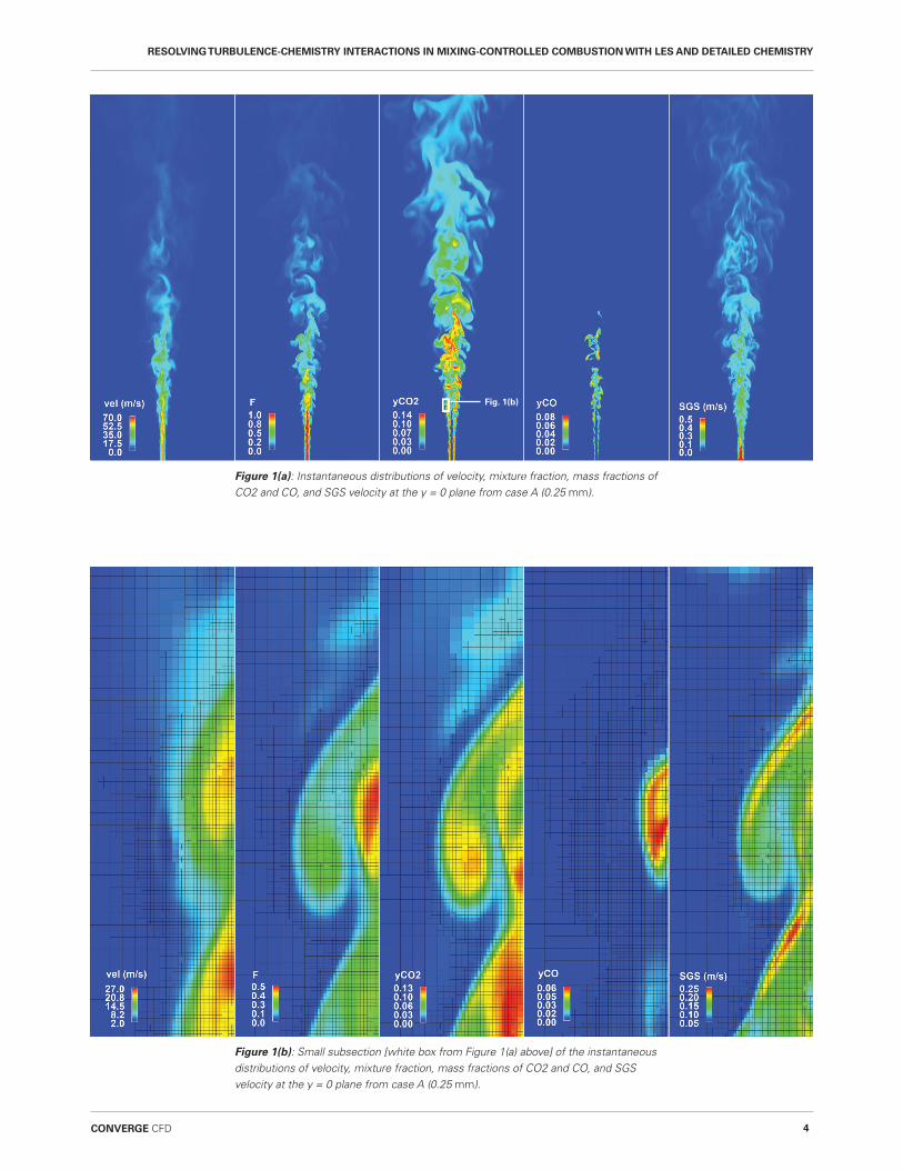
In Figure 1(a), you can see instantaneous distributions of velocity, mixture fraction, mass

fractions of CO2 and CO, and sub-grid scale (SGS) velocity (which is defined as the

square root of sub-grid scale TKE) for the case with a base grid size of 0.25 mm. You can

see spatial fine-scale structures for all of these quantities, which implies that a substantial

range of turbulent scales has been resolved.

With AMR, additional cells are added to the shear layer and to any local regions that have

large velocity gradients resulting in an effective grid size of 0.25 mm, while far away from

the shear layer the grid size remains 2 mm. Figure 1(b) expands the area of the small white

box (12 mm × 36 mm) from Figure 1(a) so that you can see the mesh around the flame.


4CONVERGE CFD

Figure 1(a): Instantaneous distributions of velocity, mixture fraction, mass fractions of CO2 and CO, and SGS velocity at the y = 0 plane from case A (0.25 mm).

Figure 1(b): Small subsection [white box from Figure 1(a) above] of the instantaneous distributions of velocity, mixture fraction, mass fractions of CO2 and CO, and SGS velocity at the y = 0 plane from case A (0.25 mm).

Fig. 1(b)



RESULTSTo obtain sufficient time-averaged statistics, LES is run for 0.35 s since flow through

the domain takes 0.02 s. Time-averaged values for mean and RMS values of velocity,

temperature, mixture fraction, and species mass fractions are calculated. Here we present

the results for the centerline of the jet and at radial positions, and we compare these simu-

lation results to experimental data17,18. Please see Liu et al., 2017 for additional results19.

GRID CONVERGENCE

To study the grid convergence of the Sandia Flame D case, we ran simulations with

minimum grid sizes from 0.25 mm (case A) to 2.0 mm (case E). Table 1 below gives

grid information for these five cases.

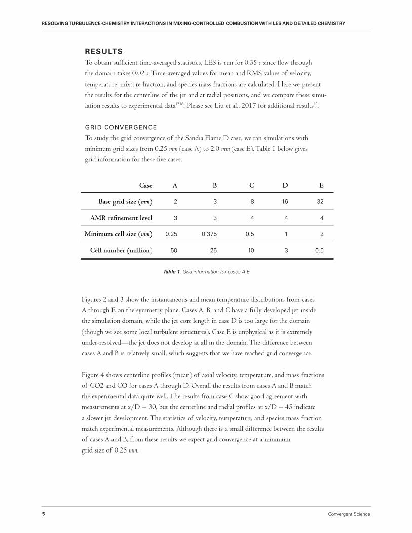
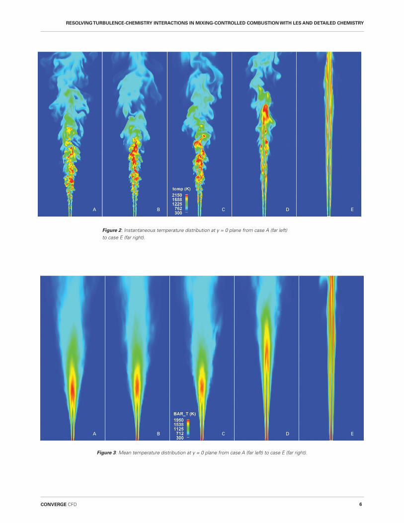
Figures 2 and 3 show the instantaneous and mean temperature distributions from cases

A through E on the symmetry plane. Cases A, B, and C have a fully developed jet inside

the simulation domain, while the jet core length in case D is too large for the domain

(though we see some local turbulent structures). Case E is unphysical as it is extremely

under-resolved—the jet does not develop at all in the domain. The difference between

cases A and B is relatively small, which suggests that we have reached grid convergence.

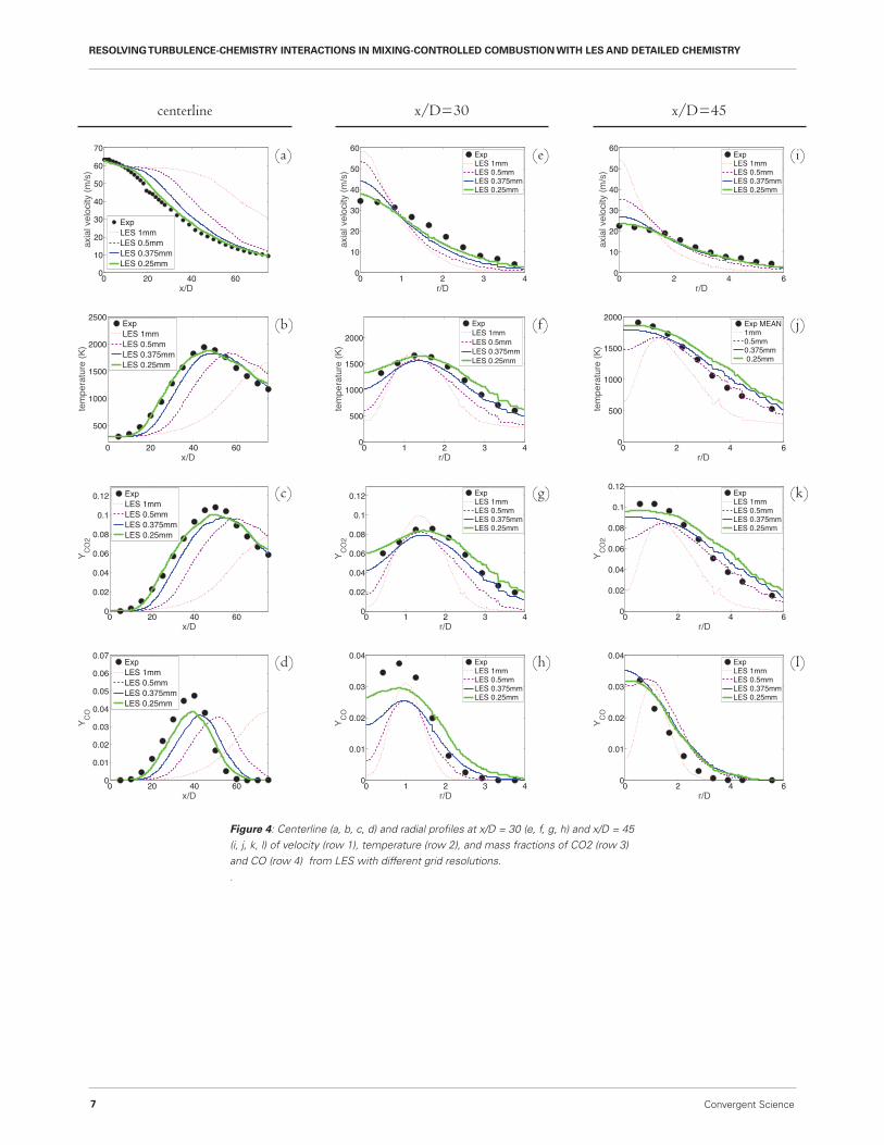
Figure 4 shows centerline profiles (mean) of axial velocity, temperature, and mass fractions

of CO2 and CO for cases A through D. Overall the results from cases A and B match

the experimental data quite well. The results from case C show good agreement with

measurements at x/D = 30, but the centerline and radial profiles at x/D = 45 indicate

a slower jet development. The statistics of velocity, temperature, and species mass fraction

match experimental measurements. Although there is a small difference between the results

of cases A and B, from these results we expect grid convergence at a minimum

grid size of 0.25 mm.

Table 1. Grid information for cases A-E

Case

Base grid size (mm)

AMR refinement level

Minimum cell size (mm)

Cell number (million)

A

2

3

0.25

50

B

3

3

0.375

25

C

8

4

0.5

10

D

16

4

1

3

E

32

4

2

0.5


6CONVERGE CFD

Figure 2: Instantaneous temperature distribution at y = 0 plane from case A (far left) to case E (far right).

Figure 3: Mean temperature distribution at y = 0 plane from case A (far left) to case E (far right).

A

A

B

B

C

C

D

D

E

E



Figure 4: Centerline (a, b, c, d) and radial profiles at x/D = 30 (e, f, g, h) and x/D = 45 (i, j, k, l) of velocity (row 1), temperature (row 2), and mass fractions of CO2 (row 3) and CO (row 4) from LES with different grid resolutions..

0 20 40 600

10

20

30

40

50

60

70

x/D

axia

l vel

ocity

(m/s

)

ExpLES 1mmLES 0.5mmLES 0.375mmLES 0.25mm

(a)

0 20 40 60

500

1000

1500

2000

2500

x/D

tem

pera

ture

(K)


(b)

0 20 40 600

0.02

0.04

0.06

0.08

0.1

0.12

x/D

Y CO

2


(c)

0 20 40 600

0.01

0.02

0.03

0.04

0.05

0.06

0.07

x/D

Y CO


(d)

0 1 2 3 40

10

20

30

40

50

60

r/D

axia

l vel

ocity

(m/s

)


(e)

0 1 2 3 40

500

1000

1500

2000

r/D

tem

pera

ture

(K)


(f)

0 1 2 3 40

0.02

0.04

0.06

0.08

0.1

0.12

r/D

Y CO

2


(g)

0 1 2 3 40

0.01

0.02

0.03

0.04

r/D

Y CO


(h)

0 2 4 60

10

20

30

40

50

60

r/D

axia

l vel

ocity

(m/s

)


(i)

0 2 4 60

500

1000

1500

2000

r/D

tem

pera

ture

(K)

Exp MEAN1mm0.5mm0.375mm 0.25mm

(j)

0 2 4 60

0.02

0.04

0.06

0.08

0.1

0.12

r/D

Y CO

2


(k)

0 2 4 60

0.01

0.02

0.03

0.04

r/D

Y CO


(l)

centerline x/D=30 x/D=45


8CONVERGE CFD

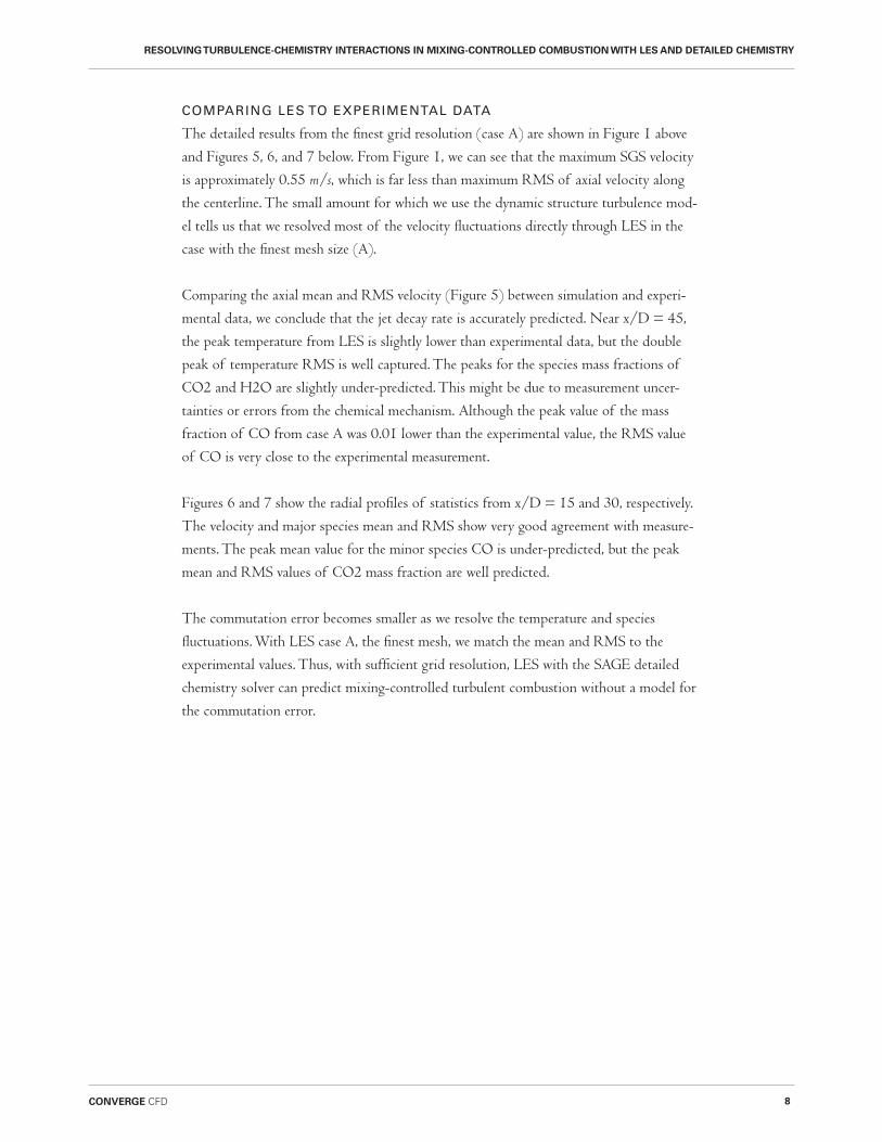
COMPARING LES TO EXPERIMENTAL DATA

The detailed results from the finest grid resolution (case A) are shown in Figure 1 above

and Figures 5, 6, and 7 below. From Figure 1, we can see that the maximum SGS velocity

is approximately 0.55 m/s, which is far less than maximum RMS of axial velocity along

the centerline. The small amount for which we use the dynamic structure turbulence mod-

el tells us that we resolved most of the velocity fluctuations directly through LES in the

case with the finest mesh size (A).

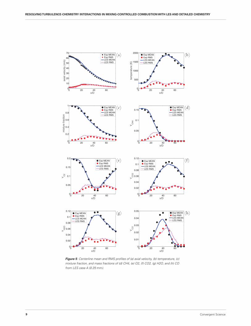
Comparing the axial mean and RMS velocity (Figure 5) between simulation and experi-

mental data, we conclude that the jet decay rate is accurately predicted. Near x/D = 45,

the peak temperature from LES is slightly lower than experimental data, but the double

peak of temperature RMS is well captured. The peaks for the species mass fractions of

CO2 and H2O are slightly under-predicted. This might be due to measurement uncer-

tainties or errors from the chemical mechanism. Although the peak value of the mass

fraction of CO from case A was 0.01 lower than the experimental value, the RMS value

of CO is very close to the experimental measurement.

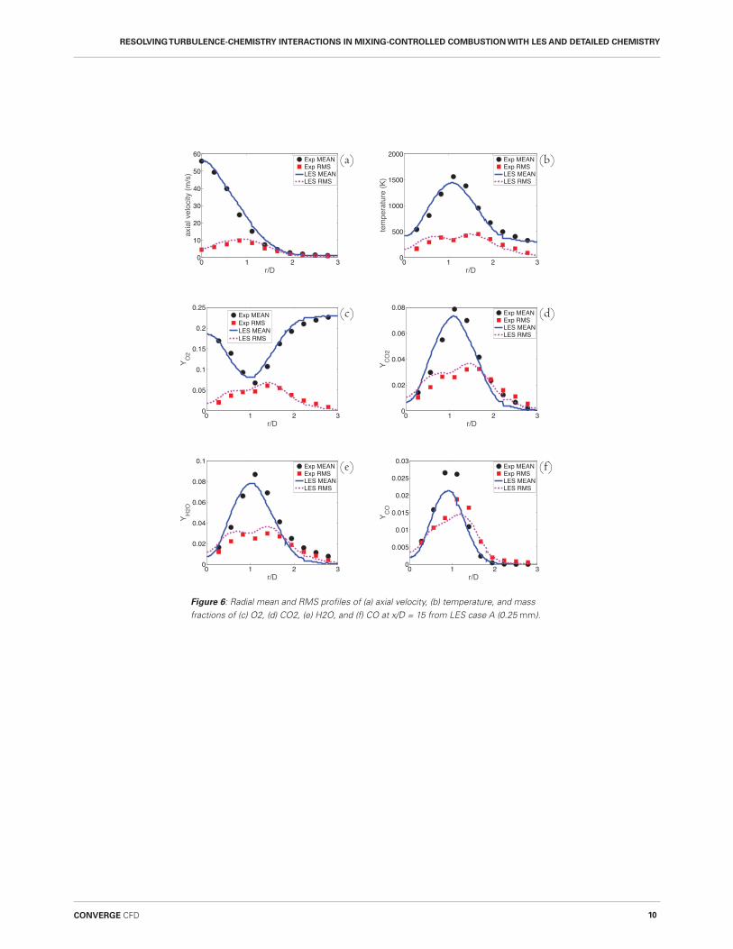
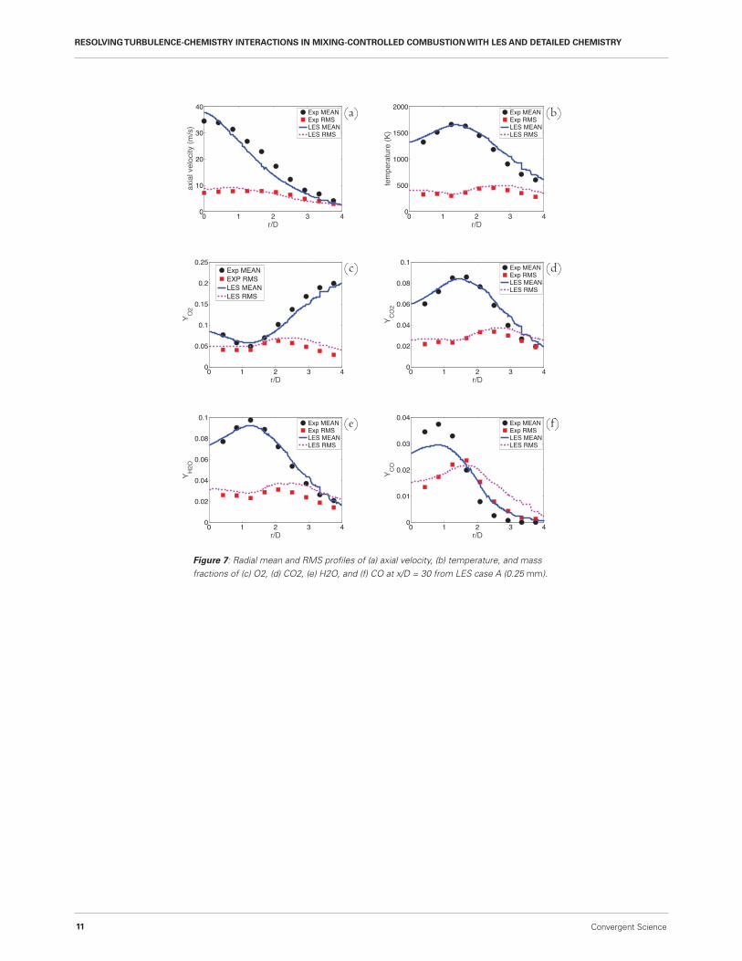
Figures 6 and 7 show the radial profiles of statistics from x/D = 15 and 30, respectively.

The velocity and major species mean and RMS show very good agreement with measure-

ments. The peak mean value for the minor species CO is under-predicted, but the peak

mean and RMS values of CO2 mass fraction are well predicted.

The commutation error becomes smaller as we resolve the temperature and species

fluctuations. With LES case A, the finest mesh, we match the mean and RMS to the

experimental values. Thus, with sufficient grid resolution, LES with the SAGE detailed

chemistry solver can predict mixing-controlled turbulent combustion without a model for

the commutation error.



Figure 5: Centerline mean and RMS profiles of (a) axial velocity, (b) temperature, (c) mixture fraction, and mass fractions of (d) CH4, (e) O2, (f) CO2, (g) H2O, and (h) CO from LES case A (0.25 mm).

0 20 40 600

10

20

30

40

50

60

70

x/D

axia

l vel

ocity

(m/s

)

Exp MEANExp RMSLES MEANLES RMS

(a)

0 20 40 600

500

1000

1500

2000

x/D

tem

pera

ture

(K)


(b)

0 20 40 600

0.05

0.1

0.15

0.2

x/D

Y O2


(e)

0 20 40 600

0.02

0.04

0.06

0.08

0.1

0.12

x/D

Y CO

2


(f)

0 20 40 600

0.2

0.4

0.6

0.8

1

x/D

mix

ture

frac

tion


(c)

0 20 40 600

0.05

0.1

0.15

x/D

Y CH

4


(d)

0 20 40 600

0.02

0.04

0.06

0.08

0.1

0.12

x/D

Y H2O


(g)

0 20 40 600

0.01

0.02

0.03

0.04

0.05

x/D

Y CO


(h)


10CONVERGE CFD

Figure 6: Radial mean and RMS profiles of (a) axial velocity, (b) temperature, and mass fractions of (c) O2, (d) CO2, (e) H2O, and (f) CO at x/D = 15 from LES case A (0.25 mm).

0 1 2 30

10

20

30

40

50

60

r/D

axia

l vel

ocity

(m/s

)


(a)

0 1 2 30

500

1000

1500

2000

r/D

tem

pera

ture

(K)


(b)

0 1 2 30

0.02

0.04

0.06

0.08

0.1

r/D

Y H2O


(e)

0 1 2 30

0.005

0.01

0.015

0.02

0.025

0.03

r/D

Y CO


(f)

0 1 2 30

0.05

0.1

0.15

0.2

0.25

r/D

Y O2


(c)

0 1 2 30

0.02

0.04

0.06

0.08

r/D

Y CO

2


(d)



Figure 7: Radial mean and RMS profiles of (a) axial velocity, (b) temperature, and mass fractions of (c) O2, (d) CO2, (e) H2O, and (f) CO at x/D = 30 from LES case A (0.25 mm).

0 1 2 3 40

10

20

30

40

r/D

axia

l vel

ocity

(m/s

)


(a)

0 1 2 3 40

500

1000

1500

2000

r/D

tem

pera

ture

(K)


(b)

0 1 2 3 40

0.02

0.04

0.06

0.08

0.1

r/D

Y H2O


(e)

0 1 2 3 40

0.01

0.02

0.03

0.04

r/D

Y CO


(f)

0 1 2 3 40

0.05

0.1

0.15

0.2

0.25

r/D

Y O2

Exp MEANEXP RMSLES MEANLES RMS

(c)

0 1 2 3 40

0.02

0.04

0.06

0.08

0.1

r/DY C

O2


(d)


12CONVERGE CFD

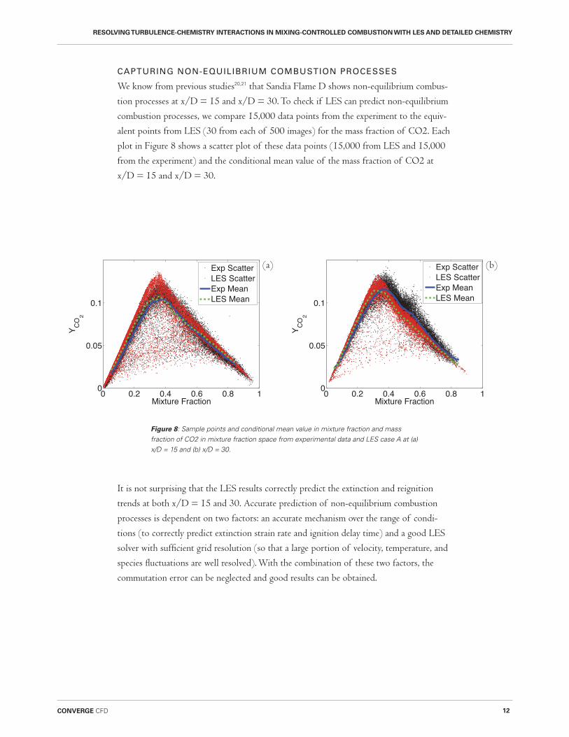
CAPTURING NON-EQUILIBRIUM COMBUSTION PROCESSES

We know from previous studies20,21 that Sandia Flame D shows non-equilibrium combus-

tion processes at x/D = 15 and x/D = 30. To check if LES can predict non-equilibrium

combustion processes, we compare 15,000 data points from the experiment to the equiv-

alent points from LES (30 from each of 500 images) for the mass fraction of CO2. Each

plot in Figure 8 shows a scatter plot of these data points (15,000 from LES and 15,000

from the experiment) and the conditional mean value of the mass fraction of CO2 at

x/D = 15 and x/D = 30.

It is not surprising that the LES results correctly predict the extinction and reignition

trends at both x/D = 15 and 30. Accurate prediction of non-equilibrium combustion

processes is dependent on two factors: an accurate mechanism over the range of condi-

tions (to correctly predict extinction strain rate and ignition delay time) and a good LES

solver with sufficient grid resolution (so that a large portion of velocity, temperature, and

species fluctuations are well resolved). With the combination of these two factors, the

commutation error can be neglected and good results can be obtained.

0 0.2 0.4 0.6 0.8 10

0.05

0.1

Mixture Fraction

Y CO

2

Exp ScatterLES ScatterExp MeanLES Mean

0 0.2 0.4 0.6 0.8 10

0.05

0.1

Mixture Fraction

Y CO

2

Exp ScatterLES ScatterExp MeanLES Mean

Figure 8: Sample points and conditional mean value in mixture fraction and mass fraction of CO2 in mixture fraction space from experimental data and LES case A at (a) x/D = 15 and (b) x/D = 30.

(a) (b)



CONCLUSIONSIn this study, we demonstrate that CONVERGE (with LES, detailed chemistry, and

sufficient grid resolution) can accurately solve a non-premixed flame without an explicit

model for the commutation error that is shown in Equation 1.

In our Sandia Flame D simulations, we find that the 0.25 mm minimum grid size is suffi-

cient to resolve most of the velocity, temperature, and species fluctuations. Adaptive Mesh

Refinement, detailed chemistry, and LES provide the simulation conditions needed to

reduce the commutation error. By resolving most of the velocity, temperature, and species

fluctuations and thereby significantly reducing the commutation error, we negate the need

for an explicit sub-grid model for the commutation error.

REFERENCES1 Drennan, S.A., and Kumar, G., “Demonstration of an Automatic Meshing Approach for Simulation of aLiquid Fueled Gas Turbine with Detailed Chemistry,” 50th AIAA/ASME/SAE/ASEE Joint Propulsion Conference, AIAA 2014-3628, Cleveland, OH, United States, July 28-30, 2014. DOI:10.2514/6.2014-3628

2 Kumar, G., and Drennan, S., “A CFD Investigation of Multiple Burner Ignition and Flame Propagation with Detailed Chemistry and Automatic Meshing,” 52nd AIAA/ SAE/ASEE Joint Propulsion Conference, Propulsion and Energy Forum, AIAA 2016- 4561, Salt Lake City, UT, United States, July 25-27, 2016. DOI:10.2514/6.2016-4561

3 Yang, S., Wang, X., Yang, V., Sun, W., and Huo, H., “Comparison of Flamelet/ Progress-Variable and Finite-Rate Chemistry LES Models in a Preconditioning Scheme,” 55th AIAA Aerospace Sciences Meeting, AIAA SciTech Forum, AIAA 2017-0605, Grapevine, TX, United States, January 9-13, 2017. DOI:10.2514/6.2017-0605

4 Pomraning, E., Richards, K., and Senecal, P.K., “Modeling Turbulent Combustion Using a RANS Model,Detailed Chemistry, and Adaptive Mesh Refinement,” SAE Paper 2014-01-1116, 2014.

5 Pei, Y., Som, S., Pomraning, E., Senecal, P.K., Skeen, S.A., Manin, J., Pickett, L.M., “Large Eddy Simulation of a Reacting Spray Flame with Multiple Realizations under Compression Ignition Engine Conditions,” Combustion and Flame, 162, 4442- 4455, 2015. DOI:10.1016/j.combustflame.2015.08.010

6 Tang, Q., Xu, J., and Pope, S.B., “Probability Density Function Calculations of Local Extinction and No Production in Piloted-jet Turbulent Methane/Air Flames,” Proceedings of the Combustion Institute, 28(1), 133–139, 2000.

7 Xu, J. and Pope, S.B., “PDF Calculations of Turbulent Nonpremixed Flames with Local Extinction,” Combustion and Flame, 123(3), 281–307, 2000.

8 Pitsch, H. and Steiner, H., “Large-Eddy Simulation of A Turbulent Piloted Methane/Air Diffusion Flame (Sandia Flame D),” Physics of Fluids, 12(10), 2541– 2554, 2000.

9 Steiner H. and Bushe, W.K., “Large Eddy Simulation of a Turbulent Reacting Jet with Conditional Source-term Estimation,” Physics of Fluids, 13(3), 754–769, 2001.

10 Barlow, R.S. Sandia National Laboratories, TNF workshop website, 2003.

11 Lu, T., and Law, C.K., “A Criterion Based on Computational Singular Perturbation for the Identification of Quasi Steady State Species: A Reduced Mechanism for Methane Oxidation with No Chemistry,” Combustion and Flame, 154(4), 761–774, 2008.


14CONVERGE CFD

12 Pomraning, E., “Development of Large Eddy Simulation Turbulence Models,” PhD thesis, University of Wisconsin–Madison, 2000.

13 Davidson, L. and Billson, M., “Hybrid LES-RANS using Synthesized Turbulent Fluctuations for Forcing in the Interface Region,” International Journal of Heat and Fluid Flow, 27(6), 1028–1042, 2006.

14 Senecal, P.K., Richards, K.J., Pomraning, E., Yang, T., Dai, M.Z., McDavid, R.M., Patterson, M.A., Hou, S., and Shethaji, T., “A New Parallel Cut-Cell Cartesian CFD Code for Rapid Grid Generation Applied to In-Cylinder Diesel Engine Simula-tions,” SAE Paper 2007-01-0159, 2007. DOI: 10.4271/2007-01-0159

15 Raju, M., Wang, M., Dai, M., Piggott, W., and Flowers, D., “Acceleration of Detailed Chemical Kinetics using Multi-zone Modeling for CFD in Internal Combustion Engine Simulations,” SAE Paper 2012-01-0135, 2012.

16 Babajimopoulos, A., Assanis, D.N., Flowers, D.L., Aceves, S.M., and Hessel, R.P., “A Fully Coupled Computational Fluid Dynamics and Multi-Zone Model with Detailed Chemical Kinetics for the Simulation of Premixed Charge Compression Ignition Engines,” International Journal of Engine Research, 6(5), 497-512, 2005.

17 Barlow R.S. and Frank J.H., “Effects of Turbulence on Species Mass Fractions in Methane/Air Jet Flames,” Symposium (International) on Combustion, 27, 1087–1095. Elsevier, 1998.

18 Nooren, P.A., Versluis, M., van der Meer, T.H., Barlow, R.S., and Frank, J.H., “Raman-Rayleigh-LIF Measurements of Temperature and Species Concentrations in the Delft Piloted Turbulent Jet Diffusion Flame,” Applied Physics B, 71(1), 95–111, 2000.

19 Liu, S., Kumar, G., Wang, M., and Pomraning, E., “Towards Accurate Tempera-ture and Species Mass Fraction Predictions for Sandia Flame-D using Detailed Chemistry and Adaptive Mesh Refinement”, 2018 AIAA Aerospace Science Meeting, AIAA 2018-1428, Kissimmee, FL, United States, January 8-12, 2018. DOI:10.2514/6.2018-1428

20 Liu, S. and Tong, C., “Investigation of Subgrid-Scale Mixing of Reactive Scalar Perturbations from Flamelets in Turbulent Partially Premixed Flames,” Combustion and Flame, 162(11), 4149–4157, 2015.

21 Liu, S. and Tong, C., “Subgrid-Scale Mixing of Mixture Fraction, Temperature, and Species Mass Fractions in Turbulent Partially Premixed Flames,” Proceedings of the Combustion Institute, 34(1), 1231–1239, 2013.

CONVERGENT SCIENCE: WORLD HEADQUARTERS6400 Enterprise LnMadison, WI 53719Tel: +1 (608) 230-1500

CONVERGENT SCIENCE: TEXAS1619 E. Common St., Suite 1204New Braunfels, TX 78130Tel: +1 (830) 625-5005

CONVERGENT SCIENCE: DETROIT21500 Haggerty Rd.Detroit, MI 48167Tel: +1 (248) 465-6005

CONVERGENT SCIENCE: EUROPEHauptstraße 10Linz, Austria 4040Tel: +43 720 010 660

CONVERGENT SCIENCE: INDIAOffice #701, Supreme Headquarters Mumbai-Bangalore Highway Baner, Pune, Maharashtra 411021+91 741-0000-870

Founded in Madison, Wisconsin, Convergent Science is a world leader in computational fluid

dynamics (CFD) software. Its flagship product, CONVERGE, includes groundbreaking technology

that eliminates the user-defined mesh, fully couples the automated mesh and the solver at runtime,

and automatically refines the mesh when and where it is needed. CONVERGE is revolutionizing

the CFD industry and shifting the paradigm toward predictive CFD.

For additional information or to contact us, visit convergecfd.com

resolving turbulence- chemistry interactions in mixing ... · resolving turbulence-chemistry...

Documents