review of probability...

Review of Probability Distributions

CS1538: Introduction to Simulations

Some Well-Known Probability Distributions

Bernoulli

Binomial

Geometric

Negative Binomial

Poisson

Uniform

Exponential

Gamma

Erlang

Gaussian/Normal

Relevance to simulations:• Need to use distributions that

are appropriate for our problem

• The closer the chosen distribution matches the distribution in reality, the more accurate our model

• Why not always make a user-defined distribution specific to our problem?

2

Discrete Distributions

Bernoulli

Binomial

Geometric

Negative Binomial

Poisson

4

The Bernoulli Distribution

5

Bernoulli Trial: an experiment with only two possible

outcomes: Success or Failure

The probability of success is p (where 0 ≤ p ≤ 1)

Let q be the probability of failure. What is q in terms of p?

Examples?

The Bernoulli Distribution

6

Let B be a random variable over the outcome of the

experiment:

B = 1 for a success; B = 0 for a failure

Expectation of B

E[B] = 1*p + 0*(1-p) = p

Variance of B

Var(B) = E[B2]- (E[B])2 = (12 p+02 (1-p)) – p2 = p – p2 = p(1– p)

Binomial Distribution

7

Experiment: Repeat Bernoulli Trial for n times

Good for determining the probability of getting k

defective items in a batch size of n

Let random variable X be the number of successes

Note: the order doesn’t matter

For example: suppose we toss a biased coin 3

times (with heads=success).

X(HHT)=2; X(THH)=2; X(HTH)=2


8

The probability mass function for X:

E[X] = E[B1 + B2 + … Bn] = S E[Bi] = np

Var(X) = Var(B1 + B2 + … Bn) = SVar(Bi) = np(1-p)

Note:

otherwise

nxqpx

n

xp

xnx

,0

,,1,0,)(

𝑛

𝑘=

𝑛!

𝑘! 𝑛 − 𝑘 !

Geometric Distribution

9

Keep on repeating Bernoulli trials until successful

Let r.v. X be the number of trials until the first

success


What is q?

otherwise

xpqxp

x

,0

,2,1,)(

1


10

E[X] = S xq(x-1)p = p S xq(x-1) = 1/p

We know that ∫ S xq(x-1) dq = S qx where x = 1,2,…

We also know that S qy for y = 0,1,2… = 1/(1-q)

So ∫ S xq(x-1) dq = 1/(1-q) – 1 = q/1-q

d/dq q/(1-q) = q/(1-q)2+ 1/(1-q) = 1/(1-q)2 = 1/p2

So p S xq(x-1) = d/dq ∫ S xq(x-1) dq = p (1/p2) = 1/p

Var(X) = q/p2

Example Question

11

Suppose a product has a p% chance of failure. What’s the

chance that it will still be working after 3 uses?

Example Question

13

What’s the chance that the product is still working after 7

uses, given that it works after 3 uses?

Geometric Distribution Properties

Pr(X > t) = qt

Memoryless

Pr(X > s+t | X > s) = Pr(X > t)

15

Negative Binomial Distribution

Keep on running Bernoulli Trials until we get k successes.

Like Geometric, but now k successes instead of 1 success

Let r.v. X be the total number of trials


Expectation: E[X] = k/p

Var(X) = kq/p2

16

otherwise

kkkxpqk

x

xp

kkx

,0

2,1,,1

1

)(

Poisson Distribution

17

Computes the probability of the number of events that

may occur in a period, given the rate of occurrence in

that period

Good for modeling arrivals

Probability mass function:

Where is a fixed value that must be positive. It represents the

average rate of the event of interest occurring.

otherwise

xx

e

xp

x

,0

,1,0,!)(

Example

The Prussian Cavalry/Horse study [Bortkiewicz, 1898; cf. Larsen&Marx]

10 cavalry corps monitored over 20 years.

X = number of fatality due to horse kicks

x = # of

deaths

Observed # of corps-years in

which x fatality occurred

Expected # of corps-year using

Poisson

0 109

1 65

2 22

3 3

4 1

Total 200

18


20

Cumulative distribution function:

Note that when x ∞, F(x) 1

𝑖=0∞ 𝑒−𝛼𝛼𝑖

𝑖!= 𝑒−𝛼 𝑖=0

∞ 𝛼𝑖

𝑖!= 𝑒−𝛼𝑒𝛼 = 1

𝐸 𝑋 = 𝛼

Var(X) =

x

i

i

i

exF

0 !)(

Example

Suppose that I see students at the rate of five per office

hours. What is the chance that I’ll see 4 students at office

hours today?

What is the chance that I’ll see less than 3 students at

office hours today?

What is the chance that I’ll see at least 3 students at

office hours today?

24

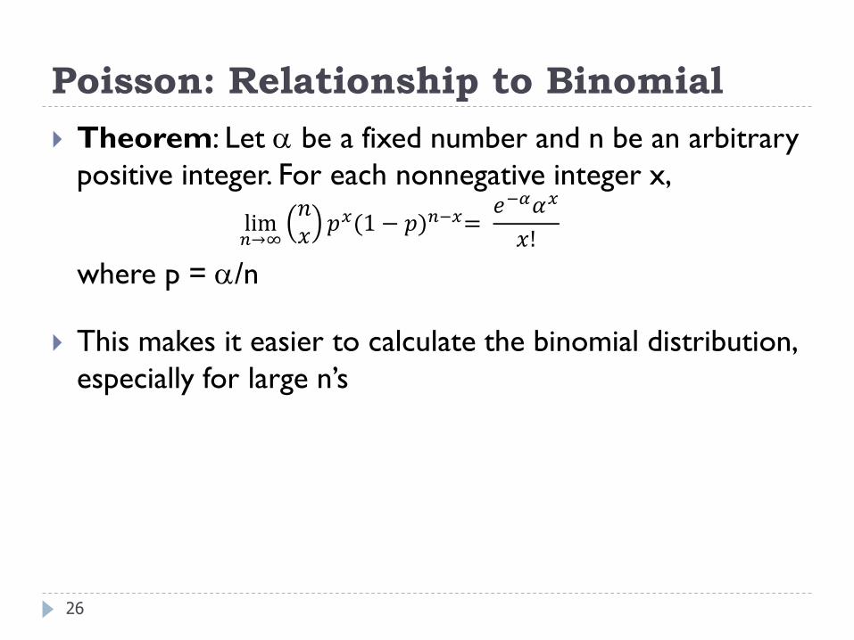
Poisson: Relationship to Binomial

Theorem: Let be a fixed number and n be an arbitrary

positive integer. For each nonnegative integer x,

lim𝑛→∞

𝑛𝑥

𝑝𝑥(1 − 𝑝)𝑛−𝑥=𝑒−𝛼𝛼𝑥

𝑥!

where p = /n

This makes it easier to calculate the binomial distribution,

especially for large n’s

26

Poisson Arrival Process

Recall represents average rate of occurrence

How do we represent time more explicitly?

Let N(t) be a random variable that represents the

number (positive integer) of events that occurred in time

[0, t]

We want to know Pr(N(t) = n)

If we guarantee a few properties, we can use the Poisson

Distribution

27

Poisson Arrival Process

Assumptions:

Arrivals occur one at a time

Arrival rate (l) does not change over time

We’ll see how to relax this

The number of arrivals in given period are independent of each

other

We can now rewrite the Poisson Distribution:

= lt

How does this affect the expectation and variance?

28

otherwise

nn

te

ntNP

nt

,0

,1,0,!

)(

])([

ll

29

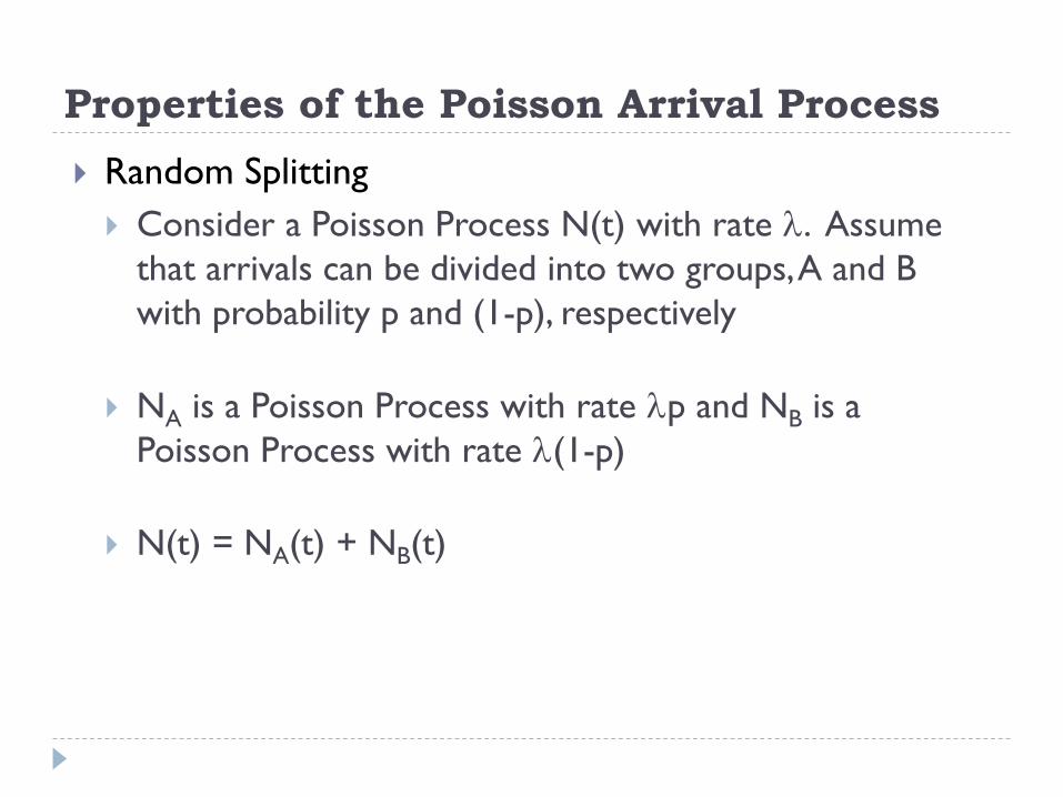
Properties of the Poisson Arrival Process

Random Splitting

Consider a Poisson Process N(t) with rate l. Assume

that arrivals can be divided into two groups, A and B

with probability p and (1-p), respectively

NA is a Poisson Process with rate lp and NB is a

Poisson Process with rate l(1-p)

N(t) = NA(t) + NB(t)

30

Properties of the Poisson Arrival Process

Pooled Process

Consider two Poisson Processes N1(t) and N2(t), with

rates l1 and l2

The sum of the two processes is also a Poisson Process;

it has a rate of l1 + l2

Pooling can be used in situations where multiple arrival

processes feed a single queue

Discrete Probability Summary



Negative Binomial Distribution


These describe experiments based on repeated Bernoulli Trials

Doesn’t have an easy to describe underlying structure, but seems to be a good fit for many real data sets

Continuous Random Variables

32

Random variable X is continuous if its range space is an

interval or a collection of intervals

There exists a non-negative function f(x), called the

probability density function, such that for any set of real

numbers,

f(x) >= 0 for all x in the range space

(i.e., the total area under f(x) is 1)

f(x) = 0 for all x not in the range space

Note that f(x) does not give the probability of X = x

Unlike the pmf for discrete random variables

spacerange

dxxf 1)(


33

The probability that X lies in a given interval [a,b] is

aka "area under the curve"

Note that for continuous random variables,

Pr(X = x) = 0 for any x

Consider the probability of x within a (very small) range

The cumulative distribution function (cdf), F(x) is now the

integral from - to x or

This gives us the probability up to x

b

adxxfbXaP )()(

x

dttfxF )()(


Expected Value for a continuous random variable

Similar to the discrete case, except that we integrate instead

of summing

Variance: same formulation as its discrete counterpart

(though calculating E[X2] will involve integrals again).

Var(X) = E[X2] – (E[X])2

dxxxfXE )(][

Uniform Distribution over range [a,b]

35

Probability density function:

Cumulative distribution function:

What about F(x) when x < a or x > b?

otherwise

bxaifabxf

0

1

)(

x

a

x

abxaif

ab

axdy

abdyyfxF

1)()(

Uniform Distribution over range [a,b]

36

Expectation

What does the expected value of a discrete uniform

distribution look like?

Variance

2)(2

))((

)(2)(2)(

222

ab

ab

abab

ab

ab

ab

x

a

bdx

ab

xXE

b

a

12

)(

)(12

)()(3)(4

4

)(

)(34

)(

)(3

])[(])[(][)(

2233

23323

22

22

ab

ab

ababab

ab

ab

abab

ab

x

a

b

XEdxab

xXEXEXVar

b

a

Normal Distribution

37


𝑓 𝑥 =1

𝜎√2𝜋exp −

1

2

𝑥−𝜇

𝜎

2, -∞ < x < ∞

where we supply the mean and variance:

m: mean

s: square-root of variance

The normal distribution is also denoted as: N(m,s2)

Some of its properties:

)())(max(

)()(

)(lim0)(lim

m

mm

fxf

xfxf

xfxf xx

Normal Distribution

38

F(x) = P(X≤x) =

Doesn’t have a closed form.

Can use numerical methods, but want to avoid evaluating

integrals for each pair (m,s2)

Transform to standard normal distribution

Let z = (t-m)/s then we can rewrite the above as:

F(x) = P(X≤x) = P(Z ≤ (x-m)/s)

=

dttx

2

2

1exp

2

1

s

m

s

dzzx

2/)(

2

1exp

2

1sm

CDF table for N(0,1)

There are a few variants. On the website:

A typical table from a stats book lets you specify z to 2 significant

digits: (z=column1+row1)

Example (from textbook 5.21)

Suppose we have a normal distribution such that:

X is a r.v. from N(50, 9)

What is the chance that X ≤ 56?

We wish to compute F(56) (i.e., P(X≤56)).

Exponential Distribution

Models

Interarrival times

Service times

Lifetime of a component that fails instantaneously

Parameter λ indicates rate



where l >0 is a parameter that we supply

Since the exponent is negative, the pdf will decrease as x increases

otherwise

xexf

x

,0

0,)(

ll


44

2

0

1)(

1][

0,1

0,0)(

l

l

l ll

XVar

XE

xedte

xxF x

xt

Exponential Distribution: l

l represents a rate: number of occurrences per time unit

x: amt. of time it took for some occurrence to take place

F(x): prob. that the event happened during interval [0,x]

1-F(x): prob. that the event doesn’t happen until after x

Example 5.17

Suppose lifespan of a type of lamp is exponentially distributed

with failure rate l = 1/3000 hrs. What’s the chance a particular

lamp will beat the average?

Has a relationship to the Poisson Arrival Process


47

Like the geometric distribution, the exponential

distribution is memoryless

P(X > s+t | X > s) = P(X > t)

The proof is similar to how we showed that the geometric

distribution is memoryless

Relationship between Poisson Distribution and

Exponential Distribution (1/3)

Events occur at a rate of l

Poisson: chance of n events taking place is given by:

Pr[N(t)=n] = e-lt (lt)n/n!

Let E be the first occurrence of an event since the start of

the clock at 0; let t represent the time when E happens

Want to find: distribution for t

Look for CDF F(t) – the probability that E happened some

time within the interval [0,t]

Then we can take the derivative of F(t) to find f(t)

Want to show: F(t) fits Exponential

Relationship between Poisson Distribution

and Exponential Distribution (2/3)

F(t) = The chance that E occurs in some interval [0,t]

= 1 – Pr(E occurred after t) = 1 – Pr(nothing took place in [0,t])

Nothing took place in [0,t] relates counting discrete event occurrences with measuring continuous time duration

Pr(nothing took place in [0,t]) = Pr[N(t)=0]

F(t) = 1 – Pr(E occurred after t) = 1 – Pr[N(t) = 0] = 1 – e–lt

which is the CDF for exponential distribution

So the duration between the 0th and 1st event of a Poisson arrival process follows an exponential distribution

Relationship between Poisson Distribution

and Exponential Distribution (3/3)

More generally, for any two events Ei and Ej that follows

the Poisson arrival process, the duration between them

also follows the exponential distribution

Let i be the time when Ei occurs and j be the time when

Ej occurs

We can use the same analysis as before (just align i with 0

and j with t in the previous case)

This is because Poisson arrival process assumes constant rate

Also makes sense – exponential distribution is memoryless

Exercises with Exponential

Rate: 0.5 arrivals per minute

F(t) = 1-e-0.5t = probability of time elapse between arrivals

What’s the probability that the next customer shows up before

30 seconds have passed?

… within 1 minute?

… within 2 minutes?

What’s the chance that a customer shows up between 5 and 7

minutes?

Relationship between Gamma Distribution

and Poisson Distribution

Suppose some event occurs over time interval of length x

at the average rate of l per unit time. How long would it

take for r events to happen?

Divide up x into small independent subintervals such that the

chance of more than one event happening in the subinterval is

negligibly small

Let W be a r.v. counting the # of occurrences of the event in

the total duration [0,x]. W is a Poisson r.v. w/ params lx

FX(x) = Pr(X≤x) = 1-Pr(X>x)

= 1-FW(r-1) =1 − 𝑘=0𝑟−1 𝑒−𝜆𝑥

(𝜆𝑥)𝑘

𝑘!

fX(x) = F’X(x) = 𝜆𝑟

𝑟−1 !𝑥𝑟−1𝑒−𝜆𝑥

The Gamma function:

If r can be non-integer, then we need to replace (r-1)! with a

continuous function of r.

We’ll call this function Gamma of r: G(r)

For any real number r > 0, the gamma function G(r) is:

Γ 𝛽 = 0

∞

𝑥𝛽−1𝑒−𝑥𝑑𝑥

G(1) = 1

G(1/2) = sqrt()

G(r+1) = r G(r) for any positive real r

G(r+1) = r! if r is a nonnegative integer

𝑛+𝑟−1

𝑛=

G(n+r)G(n+1)G(r)

G(r)G(s)G(r+s)

= 01𝑢𝑟−1(1 − 𝑢)𝑠−1𝑑𝑢

Gamma Distribution (general form) Useful for when waiting times between events is relevant (e.g.

waiting time between Poisson events)

Let X be a random variable such that

𝑓𝑋 𝑥 =

𝛽𝜃

G(β)(𝛽𝜃𝑥)𝛽−1𝑒−𝛽𝜃𝑥, 𝑥 > 0, 𝛽 > 0

0, 𝑜𝑡ℎ𝑒𝑟𝑤𝑖𝑠𝑒

𝛽 is referred to as a shape parameter

𝜃 is referred to as a scale parameter

E[X] = 0∞𝑥 𝑓 𝑥 𝑑𝑥 =

1

𝜃

Var(X) = 1

𝛽𝜃2

CDF: 𝐹𝑋 𝑥 = 0𝑥𝑓 𝑡 𝑑𝑡 = 1 − 𝑥

∞𝑓 𝑡 𝑑𝑡

Erlang Distribution

56

When β is an arbitrary positive integer, the Gamma

Distribution is called the Erlang Distribution of order k

(k= β)

Can simplify the CDF to:

𝐹 𝑋 = 1 − 𝑖=0𝑘−1 𝑒

−𝑘𝜃𝑥(𝑘𝜃𝑥)𝑖

𝑖!𝑥 > 0

0 𝑥 ≤ 0

This is the sum of Poisson terms with mean α = kθx

k is the number of events

θ is the rate of the collection of events

λ = kθ is the rate of one event (events per unit time)

Erlang Example

Suppose a node in a network does not transmit until it has

accumulated 5 messages in its buffer. Suppose messages arrive

independently and are exponentially distributed with a mean of

100 ms between messages.

Suppose a transmission was just made; what’s the probability that more

than 552 ms will pass before the next transmission?

57

review of probability...

Documents