review of the utah snow load study - utah snow load...review of the utah snow load study...
TRANSCRIPT

Review of the Utah Snow Load Study
Brennan Bean, Marc Maguire, and Yan Sun
Utah State University
February 14th, 2018
Bean, Maguire, and Sun Utah Snow Load Study February 14th, 2018 1 / 71
Outline
1 Introduction
2 Data Set Development
3 Spatial MethodsInverse Distance Weighting (IDW)Linear Triangulation Interpolation (TRI)PRISMKriging
4 Visual Comparisons
5 Cross Validation
6 Applications
7 Acknowledgements and References
Bean, Maguire, and Sun Utah Snow Load Study February 14th, 2018 2 / 71

IntroductionThe Snow Load Challenge
Proper consideration of snow loads inbuilding design can be a delicatebalancing act:
Underestimates → structurefailure
Overestimates → increasedconstruction costs
Figure 1: Minneapolis Metrodome, December2010[8].
Bean, Maguire, and Sun Utah Snow Load Study February 14th, 2018 3 / 71
IntroductionThe Snow Load Challenge
Proper consideration of snow loads inbuilding design can be a delicatebalancing act:
Underestimates → structurefailure
Overestimates → increasedconstruction costs
Figure 2: Cost of roof joists built for varioussnow loads. (Courtesy of Vulcraft).
Bean, Maguire, and Sun Utah Snow Load Study February 14th, 2018 4 / 71
IntroductionThe Snow Load Challenge
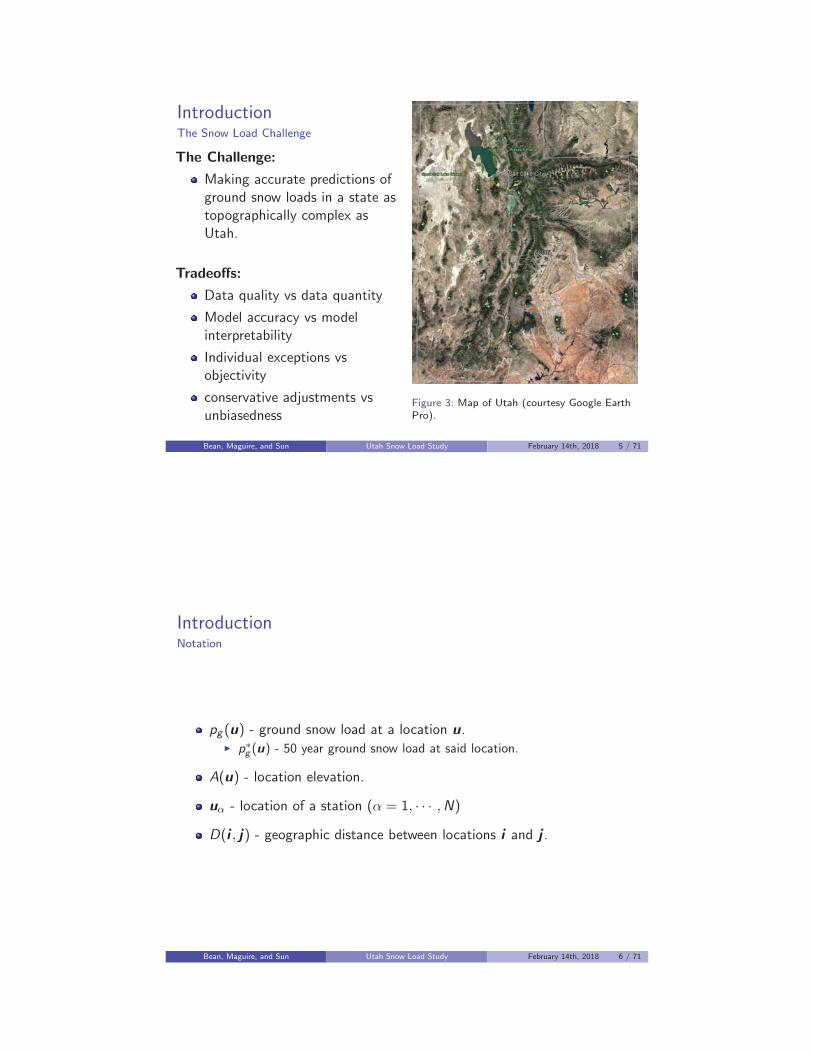
The Challenge:
Making accurate predictions ofground snow loads in a state astopographically complex asUtah.
Tradeoffs:
Data quality vs data quantity
Model accuracy vs modelinterpretability
Individual exceptions vsobjectivity
conservative adjustments vsunbiasedness
Figure 3: Map of Utah (courtesy Google EarthPro).
Bean, Maguire, and Sun Utah Snow Load Study February 14th, 2018 5 / 71
IntroductionNotation
pg (u) - ground snow load at a location u.� p∗g (u) - 50 year ground snow load at said location.
A(u) - location elevation.
uα - location of a station (α = 1, · · · ,N)
D(i , j ) - geographic distance between locations i and j .
Bean, Maguire, and Sun Utah Snow Load Study February 14th, 2018 6 / 71
IntroductionUtah ground snow loads
Most recent Utah snow load report created in 1990 (updated in 1992)[12].
Prediction equations intended to capture a near upper bound forground snow loads at any given elevation within each county.
Pg (u) =
⎧⎨⎩(P20 + S2 (A(u)− A0)
2) 1
2A(u) > A0
P0 A(u) ≤ A0
County specific parameters:
P0 - base ground snow load
S - change in ground snow load with elevation
A0 - (base ground snow elevation)
Bean, Maguire, and Sun Utah Snow Load Study February 14th, 2018 7 / 71
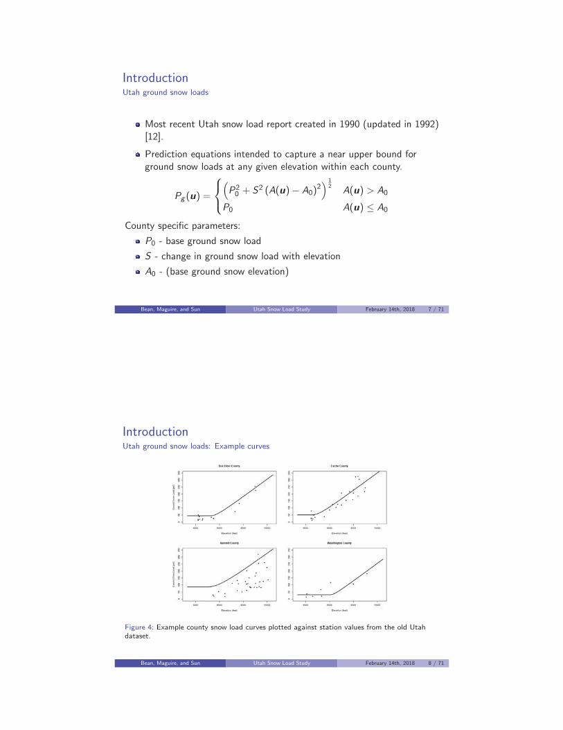
IntroductionUtah ground snow loads: Example curves
Figure 4: Example county snow load curves plotted against station values from the old Utahdataset.
Bean, Maguire, and Sun Utah Snow Load Study February 14th, 2018 8 / 71
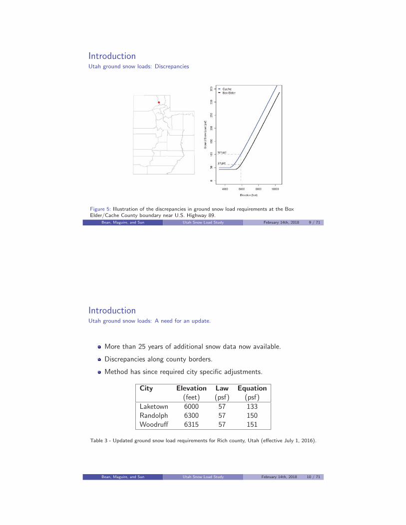
IntroductionUtah ground snow loads: Discrepancies
Figure 5: Illustration of the discrepancies in ground snow load requirements at the BoxElder/Cache County boundary near U.S. Highway 89.
Bean, Maguire, and Sun Utah Snow Load Study February 14th, 2018 9 / 71
IntroductionUtah ground snow loads: A need for an update.
More than 25 years of additional snow data now available.
Discrepancies along county borders.
Method has since required city specific adjustments.
City Elevation Law Equation(feet) (psf) (psf)
Laketown 6000 57 133Randolph 6300 57 150Woodruff 6315 57 151
Table 3 - Updated ground snow load requirements for Rich county, Utah (effective July 1, 2016).
Bean, Maguire, and Sun Utah Snow Load Study February 14th, 2018 10 / 71
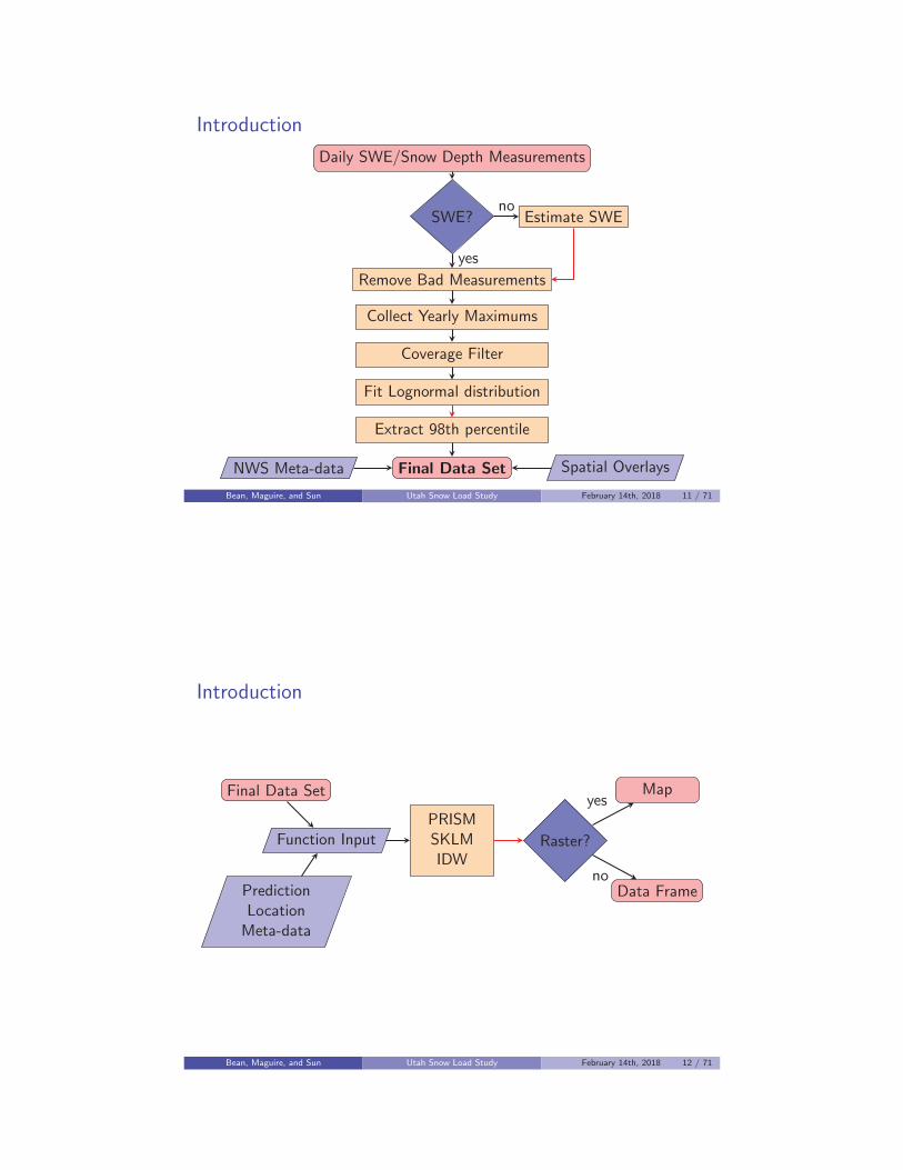
Introduction
Daily SWE/Snow Depth Measurements
SWE? Estimate SWE
Remove Bad Measurements
Collect Yearly Maximums
Coverage Filter
Fit Lognormal distribution
Extract 98th percentile
Final Data SetNWS Meta-data Spatial Overlays
no
yes
Bean, Maguire, and Sun Utah Snow Load Study February 14th, 2018 11 / 71
Introduction
Final Data Set
PredictionLocationMeta-data
Function InputPRISMSKLMIDW
Raster?
Map
Data Frame
yes
no
Bean, Maguire, and Sun Utah Snow Load Study February 14th, 2018 12 / 71
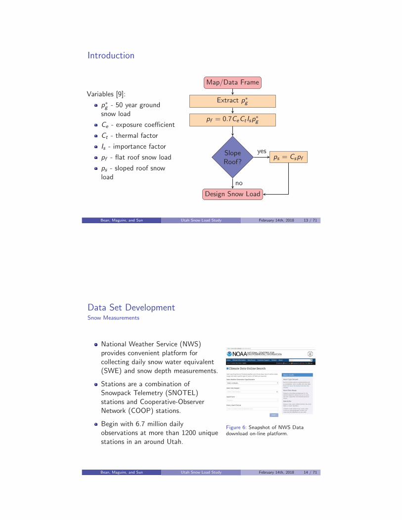
Introduction
Variables [9]:
p∗g - 50 year groundsnow load
Ce - exposure coefficient
Ct - thermal factor
Is - importance factor
pf - flat roof snow load
ps - sloped roof snowload
Map/Data Frame
Extract p∗g
pf = 0.7CeCt Isp∗g
SlopeRoof?
ps = Cspf
Design Snow Load
no
yes
Bean, Maguire, and Sun Utah Snow Load Study February 14th, 2018 13 / 71
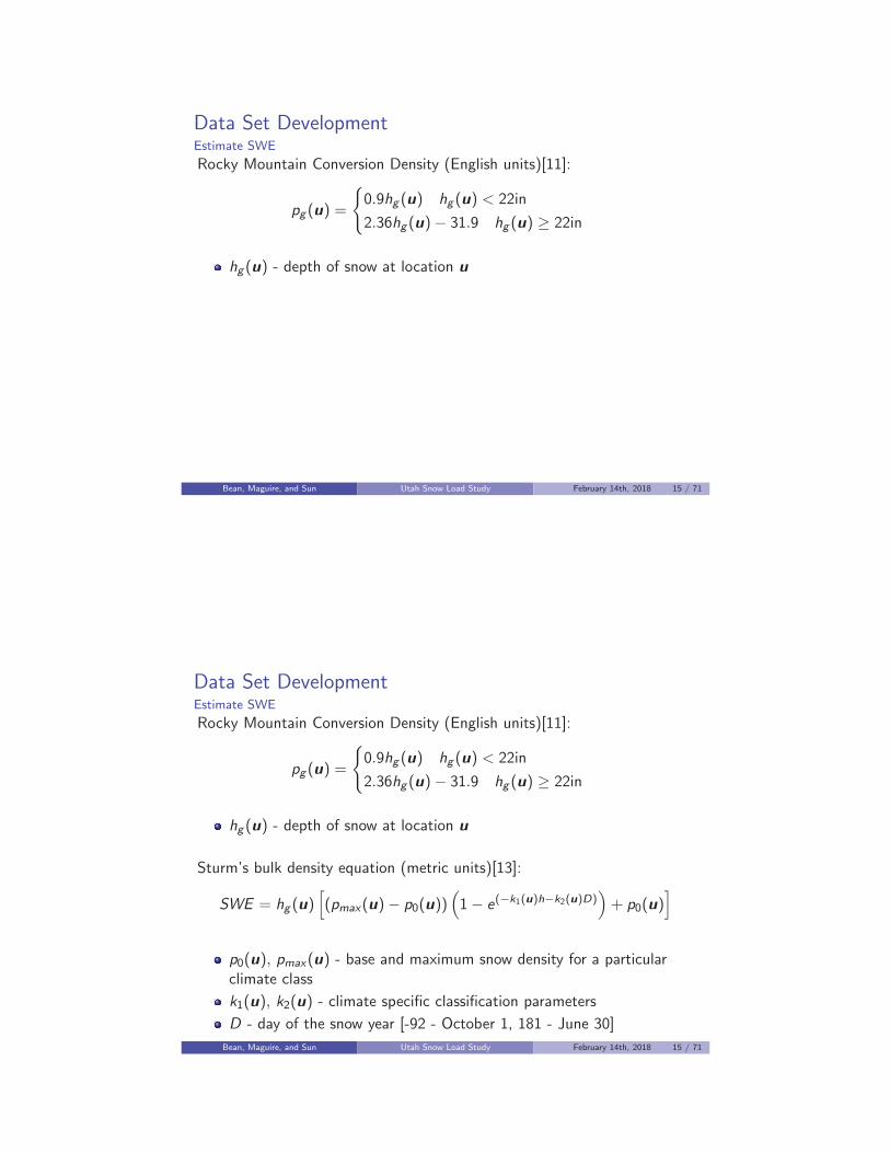
Data Set DevelopmentSnow Measurements
National Weather Service (NWS)provides convenient platform forcollecting daily snow water equivalent(SWE) and snow depth measurements.
Stations are a combination ofSnowpack Telemetry (SNOTEL)stations and Cooperative-ObserverNetwork (COOP) stations.
Begin with 6.7 million dailyobservations at more than 1200 uniquestations in an around Utah.
Figure 6: Snapshot of NWS Datadownload on-line platform.
Bean, Maguire, and Sun Utah Snow Load Study February 14th, 2018 14 / 71
Data Set DevelopmentEstimate SWE
Rocky Mountain Conversion Density (English units)[11]:
pg (u) =
{0.9hg (u) hg (u) < 22in
2.36hg (u)− 31.9 hg (u) ≥ 22in
hg (u) - depth of snow at location u
Bean, Maguire, and Sun Utah Snow Load Study February 14th, 2018 15 / 71
Data Set DevelopmentEstimate SWE
Rocky Mountain Conversion Density (English units)[11]:
pg (u) =
{0.9hg (u) hg (u) < 22in
2.36hg (u)− 31.9 hg (u) ≥ 22in
hg (u) - depth of snow at location u
Sturm’s bulk density equation (metric units)[13]:
SWE = hg (u)[(pmax(u)− p0(u))
(1− e(−k1(u)h−k2(u)D)
)+ p0(u)
]
p0(u), pmax(u) - base and maximum snow density for a particularclimate class
k1(u), k2(u) - climate specific classification parameters
D - day of the snow year [-92 - October 1, 181 - June 30]
Bean, Maguire, and Sun Utah Snow Load Study February 14th, 2018 15 / 71
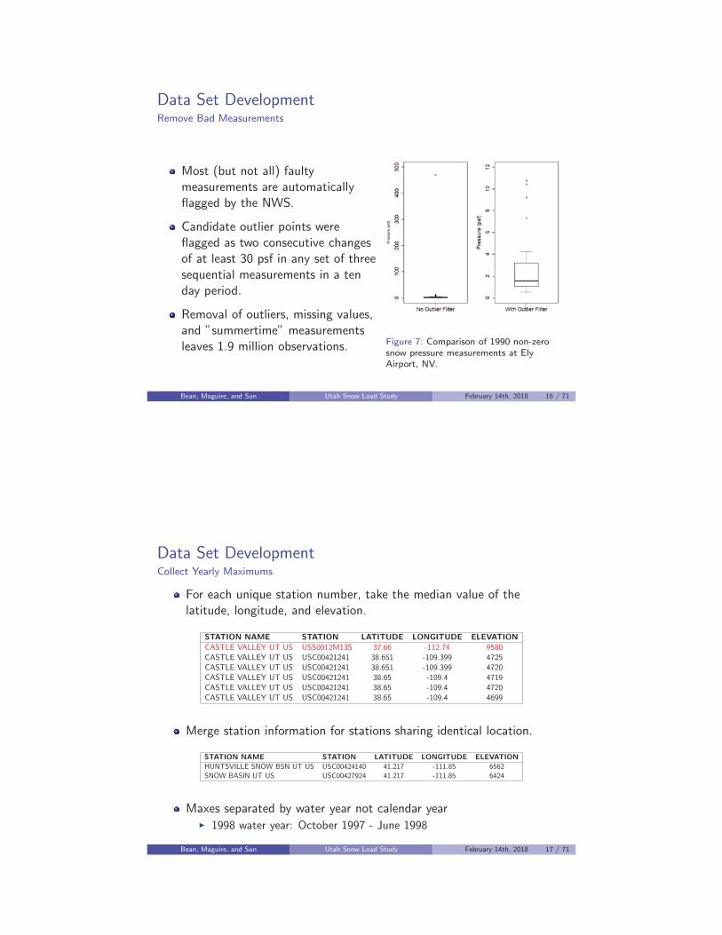
Data Set DevelopmentRemove Bad Measurements
Most (but not all) faultymeasurements are automaticallyflagged by the NWS.
Candidate outlier points wereflagged as two consecutive changesof at least 30 psf in any set of threesequential measurements in a tenday period.
Removal of outliers, missing values,and ”summertime” measurementsleaves 1.9 million observations. Figure 7: Comparison of 1990 non-zero
snow pressure measurements at ElyAirport, NV.
Bean, Maguire, and Sun Utah Snow Load Study February 14th, 2018 16 / 71
Data Set DevelopmentCollect Yearly Maximums
For each unique station number, take the median value of thelatitude, longitude, and elevation.
STATION NAME STATION LATITUDE LONGITUDE ELEVATIONCASTLE VALLEY UT US USS0012M13S 37.66 -112.74 9580CASTLE VALLEY UT US USC00421241 38.651 -109.399 4725CASTLE VALLEY UT US USC00421241 38.651 -109.399 4720CASTLE VALLEY UT US USC00421241 38.65 -109.4 4719CASTLE VALLEY UT US USC00421241 38.65 -109.4 4720CASTLE VALLEY UT US USC00421241 38.65 -109.4 4699
Merge station information for stations sharing identical location.
STATION NAME STATION LATITUDE LONGITUDE ELEVATIONHUNTSVILLE SNOW BSN UT US USC00424140 41.217 -111.85 6562SNOW BASIN UT US USC00427924 41.217 -111.85 6424
Maxes separated by water year not calendar year� 1998 water year: October 1997 - June 1998
Bean, Maguire, and Sun Utah Snow Load Study February 14th, 2018 17 / 71

Data Set DevelopmentApply Coverage Filter
Distribution fitting techniqueassumes all maximums atlocation u come from the samelog-normal distribution.
Inadequate coverage of the snowseason introduces low outliers tothe distribution fitting process.
Low outliers artificially inflatethe standard deviationparameter of the log-normaldistribution.
� In this example, σlog = 0.69 vsσlog = 0.33.
Figure 8: Theoretical log-normal distributionquantiles vs empirical (observed) quantiles for(a) raw yearly maximum snow loads and (b)yearly maximums with coverage filter applied inLevan, UT.
Bean, Maguire, and Sun Utah Snow Load Study February 14th, 2018 18 / 71
Data Set DevelopmentApply Coverage Filter
Coverage filter designed toensure measurements representtrue yearly maximums.
� Low Elevations - December toMarch
� High Elevations - February toMay
Maximum only retained if thereare measurements taken in allfour months specified above ORmaximum is in the upper half ofall yearly maximums for thatstation.
Throwing out bottom 10% ofdata for each station also guardsagainst low outliers.
Figure 9: Month in which yearly maximumground snow load occurred as separated byelevation.
Bean, Maguire, and Sun Utah Snow Load Study February 14th, 2018 19 / 71
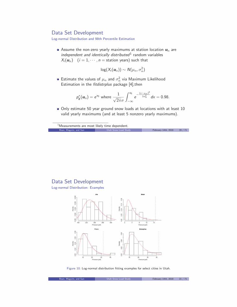
Data Set DevelopmentLog-normal Distribution and 98th Percentile Estimation
Assume the non-zero yearly maximums at station location uα areindependent and identically distributed1 random variablesXi (uα) (i = 1, · · · , n = station years) such that
log(Xi (uα)) ∼ N(μα, σ2α)
Estimate the values of μα and σ2α via Maximum Likelihood
Estimation in the fitdistrplus package [4],then
p∗g (uα) = ex0 where1√2πσ
∫ x0
−∞e− (x−μα)2
2σ2α dx = 0.98.
Only estimate 50 year ground snow loads at locations with at least 10valid yearly maximums (and at least 5 nonzero yearly maximums).
1Measurements are most likely time dependent.Bean, Maguire, and Sun Utah Snow Load Study February 14th, 2018 20 / 71
Data Set DevelopmentLog-normal Distribution: Examples
Figure 10: Log-normal distribution fitting examples for select cities in Utah.
Bean, Maguire, and Sun Utah Snow Load Study February 14th, 2018 21 / 71
Summary of MethodsInverse Distance Weighting (IDW)
p∗g (u) =A(u)∑N
α=1D (uα,u)
n∑α=1
[(1
D (uα,u)
)c p∗g (uα)
A(uα)
].
c - weighting exponent for distance weighting
NGSL =p∗g (uα)
A(uα)is commonly used method to account for elevation in
predictions� ”reduce[s] the entire area to a common base elevation” [10].
� Used in the current snow load reports of Idaho, Montana, andWashington [10].
Bean, Maguire, and Sun Utah Snow Load Study February 14th, 2018 22 / 71
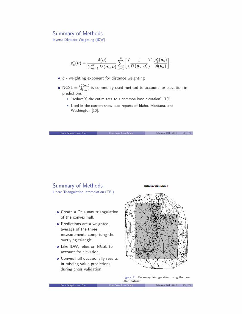
Summary of MethodsLinear Triangulation Interpolation (TRI)
Create a Delaunay triangulationof the convex hull.
Predictions are a weightedaverage of the threemeasurements comprising theoverlying triangle.
Like IDW, relies on NGSL toaccount for elevation.
Convex hull occasionally resultsin missing value predictionsduring cross validation.
Figure 11: Delaunay triangulation using the newUtah dataset
LognBean, Maguire, and Sun Utah Snow Load Study February 14th, 2018 23 / 71
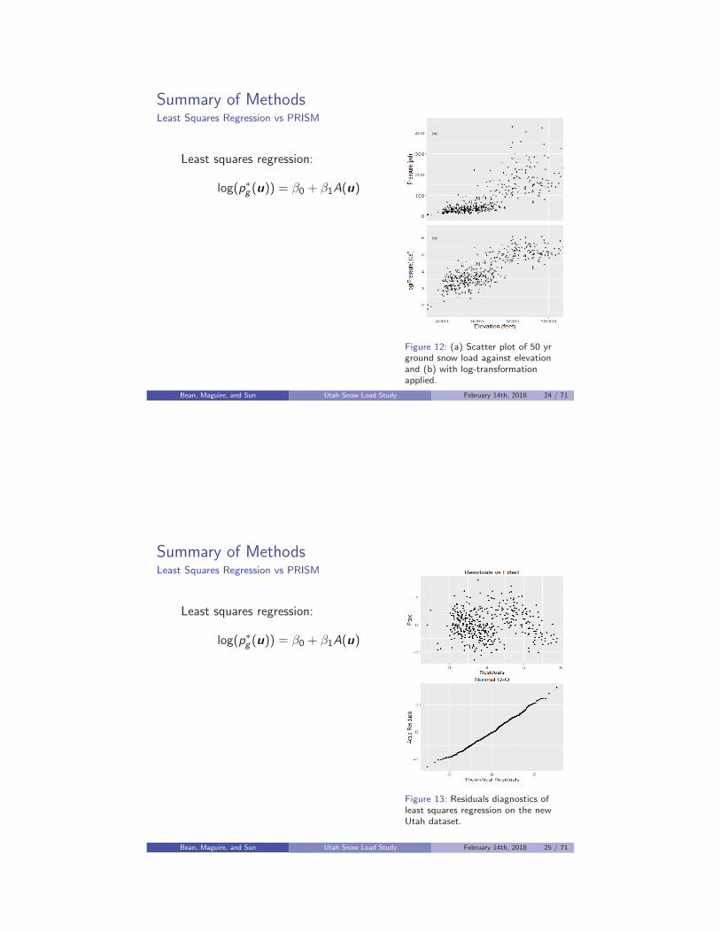
Summary of MethodsLeast Squares Regression vs PRISM
Least squares regression:
log(p∗g (u)) = β0 + β1A(u)
Figure 12: (a) Scatter plot of 50 yrground snow load against elevationand (b) with log-transformationapplied.
Bean, Maguire, and Sun Utah Snow Load Study February 14th, 2018 24 / 71
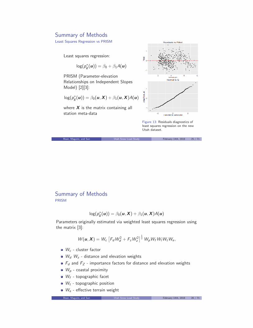
Summary of MethodsLeast Squares Regression vs PRISM
Least squares regression:
log(p∗g (u)) = β0 + β1A(u)
Figure 13: Residuals diagnostics ofleast squares regression on the newUtah dataset.
Bean, Maguire, and Sun Utah Snow Load Study February 14th, 2018 25 / 71
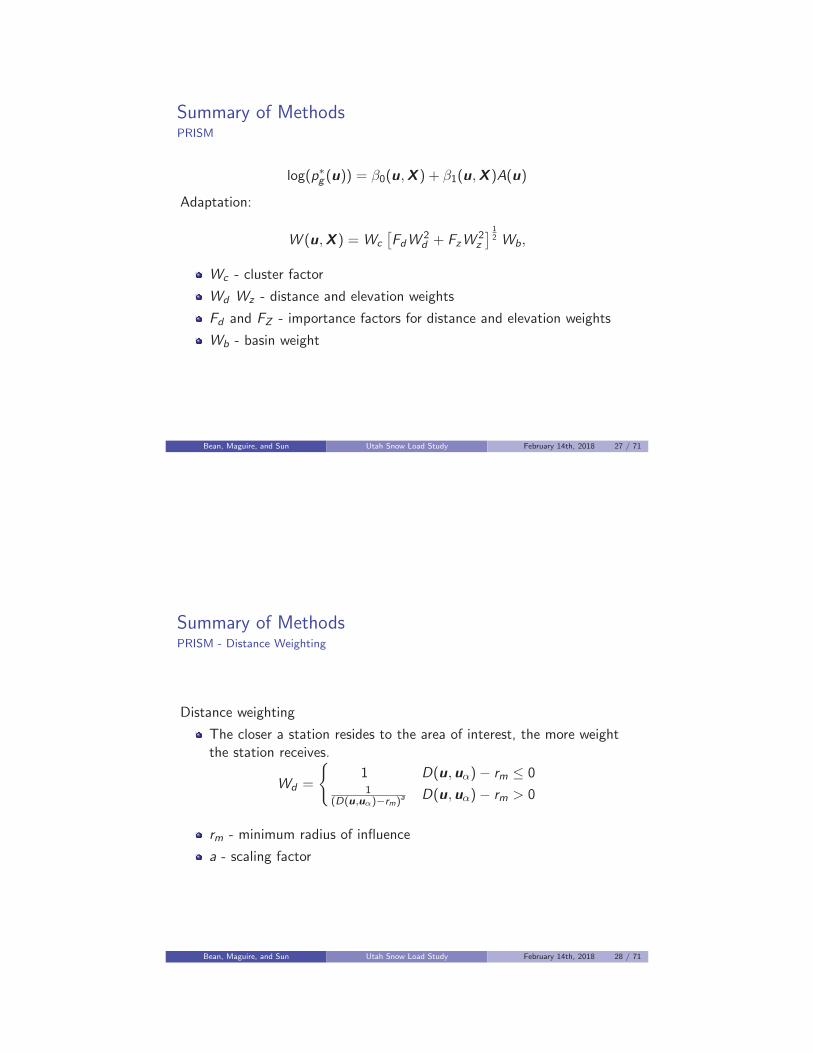
Summary of MethodsLeast Squares Regression vs PRISM
Least squares regression:
log(p∗g (u)) = β0 + β1A(u)
PRISM (Parameter-elevationRelationships on Independent SlopesModel) [2][3]:
log(p∗g (u)) = β0(u,X ) + β1(u,X )A(u)
where X is the matrix containing allstation meta-data
Figure 13: Residuals diagnostics ofleast squares regression on the newUtah dataset.
Bean, Maguire, and Sun Utah Snow Load Study February 14th, 2018 25 / 71
Summary of MethodsPRISM
log(p∗g (u)) = β0(u,X ) + β1(u,X )A(u)
Parameters originally estimated via weighted least squares regression usingthe matrix [3]:
W (u,X ) = Wc
[FdW
2d + FzW
2z
] 12 WpWfWlWtWe ,
Wc - cluster factor
Wd Wz - distance and elevation weights
Fd and FZ - importance factors for distance and elevation weights
Wp - coastal proximity
Wf - topographic facet
Wt - topographic position
We - effective terrain weight
Bean, Maguire, and Sun Utah Snow Load Study February 14th, 2018 26 / 71
Summary of MethodsPRISM
log(p∗g (u)) = β0(u,X ) + β1(u,X )A(u)
Adaptation:
W (u,X ) = Wc
[FdW
2d + FzW
2z
] 12 Wb,
Wc - cluster factor
Wd Wz - distance and elevation weights
Fd and FZ - importance factors for distance and elevation weights
Wb - basin weight
Bean, Maguire, and Sun Utah Snow Load Study February 14th, 2018 27 / 71
Summary of MethodsPRISM - Distance Weighting
Distance weighting
The closer a station resides to the area of interest, the more weightthe station receives.
Wd =
{1 D(u,uα)− rm ≤ 01
(D(u,uα)−rm)a D(u,uα)− rm > 0
rm - minimum radius of influence
a - scaling factor
Bean, Maguire, and Sun Utah Snow Load Study February 14th, 2018 28 / 71

Summary of MethodsPRISM - Elevation Weighting
Elevation weighting
Stations with similar elevations to the area of interest receive moreweight
Wz =
⎧⎪⎪⎨⎪⎪⎩
1(Δzm)
b Δz ≤ Δzm1
(Δz)bΔzm < Δz < Δzx
0 Δz ≥ Δzx
Δz = |A(u)− A(uα)|Δzm,Δzx - minimum and maximum elevation differences (userspecified).
b - scaling factor
Bean, Maguire, and Sun Utah Snow Load Study February 14th, 2018 29 / 71
Summary of MethodsPRISM - Basin Weighting
Basin Weighting
Use water catchments as a replacement fortopographic facet.
USGS Hydro-logic unit code (HUC) are 12-digitnumbers, with every two digits representing a smallerwater catchment (left to right).
Wb =
(sα + 1
5
)c
sα - number of common watersheds (four levelsranging from HUC 2 through 8) shared by uα and uc - scaling factor
Figure 14: Samplewater basins inUtah [16].
Bean, Maguire, and Sun Utah Snow Load Study February 14th, 2018 30 / 71
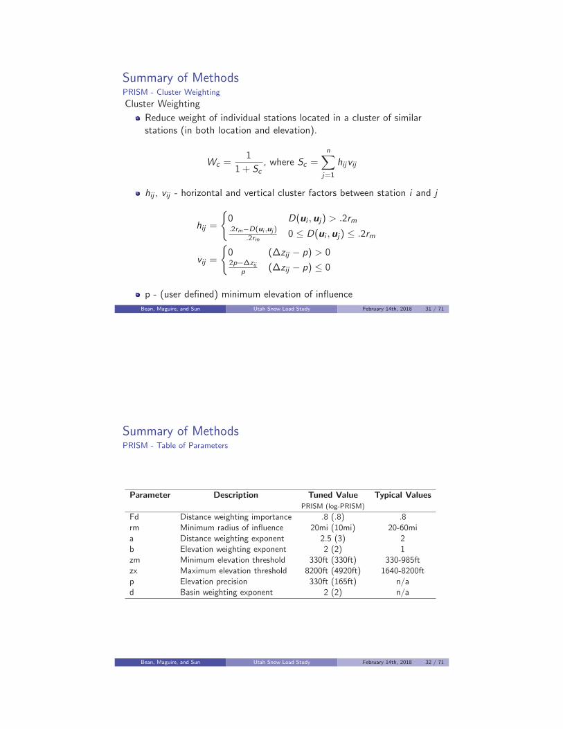
Summary of MethodsPRISM - Cluster Weighting
Cluster Weighting
Reduce weight of individual stations located in a cluster of similarstations (in both location and elevation).
Wc =1
1 + Sc, where Sc =
n∑j=1
hijvij
hij , vij - horizontal and vertical cluster factors between station i and j
hij =
{0 D(ui ,uj) > .2rm.2rm−D(ui ,uj )
.2rm0 ≤ D(ui ,uj) ≤ .2rm
vij =
{0 (Δzij − p) > 02p−Δzij
p (Δzij − p) ≤ 0
p - (user defined) minimum elevation of influence
Bean, Maguire, and Sun Utah Snow Load Study February 14th, 2018 31 / 71
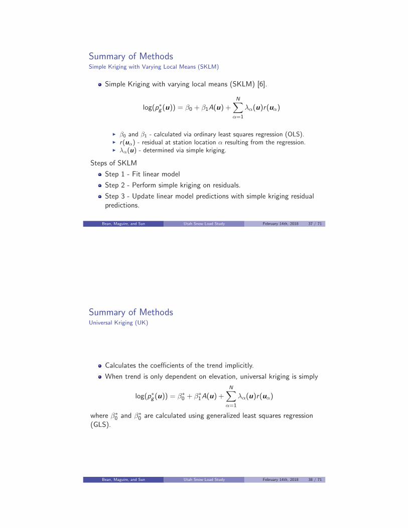
Summary of MethodsPRISM - Table of Parameters
Parameter Description Tuned Value Typical ValuesPRISM (log-PRISM)
Fd Distance weighting importance .8 (.8) .8rm Minimum radius of influence 20mi (10mi) 20-60mia Distance weighting exponent 2.5 (3) 2b Elevation weighting exponent 2 (2) 1zm Minimum elevation threshold 330ft (330ft) 330-985ftzx Maximum elevation threshold 8200ft (4920ft) 1640-8200ftp Elevation precision 330ft (165ft) n/ad Basin weighting exponent 2 (2) n/a
Bean, Maguire, and Sun Utah Snow Load Study February 14th, 2018 32 / 71

Bean, Maguire, and Sun Utah Snow Load Study February 14th, 2018 33 / 71
Summary of MethodsKriging
Considering the random function Z (u), all kriging estimators have theform1
Z (u∗) =N∑
α=1
λαZ (uα), λα ∈ R,
where the λ′i s form the unbiased estimator of Z (u) that minimizes
Q(λ) = E(Z (u∗)− Z (u∗)
)2i.e.
∑α
∑β
λαλβCZ (uα − uβ)− 2∑α
λαCZ (uα − u∗) + CZ (0)
where CZ (ui − uj) = Cov(Z (ui ),Z (uj)).
1references [5] and [7] motivate this notationBean, Maguire, and Sun Utah Snow Load Study February 14th, 2018 34 / 71

Summary of MethodsSimple Kriging
We can minimize Q(u) by ∇Q(λ) = 0 i.e.∑α
λαCZ (uα − uβ) = CZ (uβ − u∗) β = 1, · · · , n.
When the following conditions are met:
1 E (Z (u)) = m is constant over the entire region of interest.
2 C (h) = Cov (Z (u + h),Z (u)) is independent of location u.
Bean, Maguire, and Sun Utah Snow Load Study February 14th, 2018 35 / 71
Summary of MethodsVariograms
Define
γ(h) =1
2Var [Z (u + h)− Z (u)]
Estimated by
γ(h) =1
2Nh
Nh∑αh=1
[Z (uαh+ h)− Z (uαh
)]2
where Nh is the number of stations hdistance apart from each other.
Under certain conditions:γ(h) = C (0)− C (h) Figure 15: Empirical semi-variances for the
residuals of station ground snow loads resultingfrom Ordinary Least Squares Regression (OLS).
Bean, Maguire, and Sun Utah Snow Load Study February 14th, 2018 36 / 71
Summary of MethodsSimple Kriging with Varying Local Means (SKLM)
Simple Kriging with varying local means (SKLM) [6].
log(p∗g (u)) = β0 + β1A(u) +N∑
α=1
λα(u)r(uα)
� β0 and β1 - calculated via ordinary least squares regression (OLS).� r(uα) - residual at station location α resulting from the regression.� λα(u) - determined via simple kriging.
Steps of SKLM
Step 1 - Fit linear model
Step 2 - Perform simple kriging on residuals.
Step 3 - Update linear model predictions with simple kriging residualpredictions.
Bean, Maguire, and Sun Utah Snow Load Study February 14th, 2018 37 / 71
Summary of MethodsUniversal Kriging (UK)
Calculates the coefficients of the trend implicitly.
When trend is only dependent on elevation, universal kriging is simply
log(p∗g (u)) = β∗0 + β∗
1A(u) +N∑
α=1
λα(u)r(uα)
where β∗0 and β∗
0 are calculated using generalized least squares regression(GLS).
Bean, Maguire, and Sun Utah Snow Load Study February 14th, 2018 38 / 71
Summary of MethodsOLS vs GLS
Figure 16: Regression curve estimates for (a) the new Utah dataset and (b) the old Utah dataset.
Bean, Maguire, and Sun Utah Snow Load Study February 14th, 2018 39 / 71
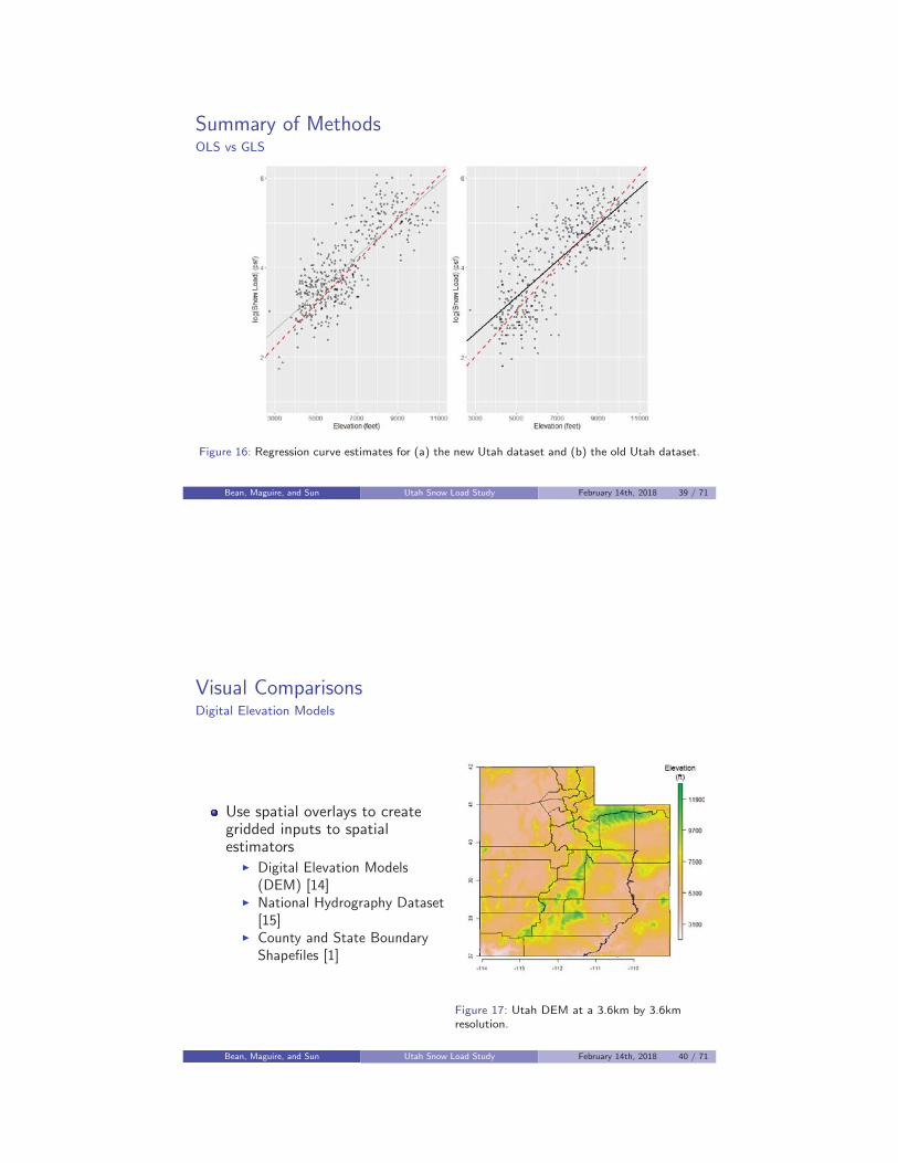
Visual ComparisonsDigital Elevation Models
Use spatial overlays to creategridded inputs to spatialestimators
� Digital Elevation Models(DEM) [14]
� National Hydrography Dataset[15]
� County and State BoundaryShapefiles [1]
Figure 17: Utah DEM at a 3.6km by 3.6kmresolution.
Bean, Maguire, and Sun Utah Snow Load Study February 14th, 2018 40 / 71
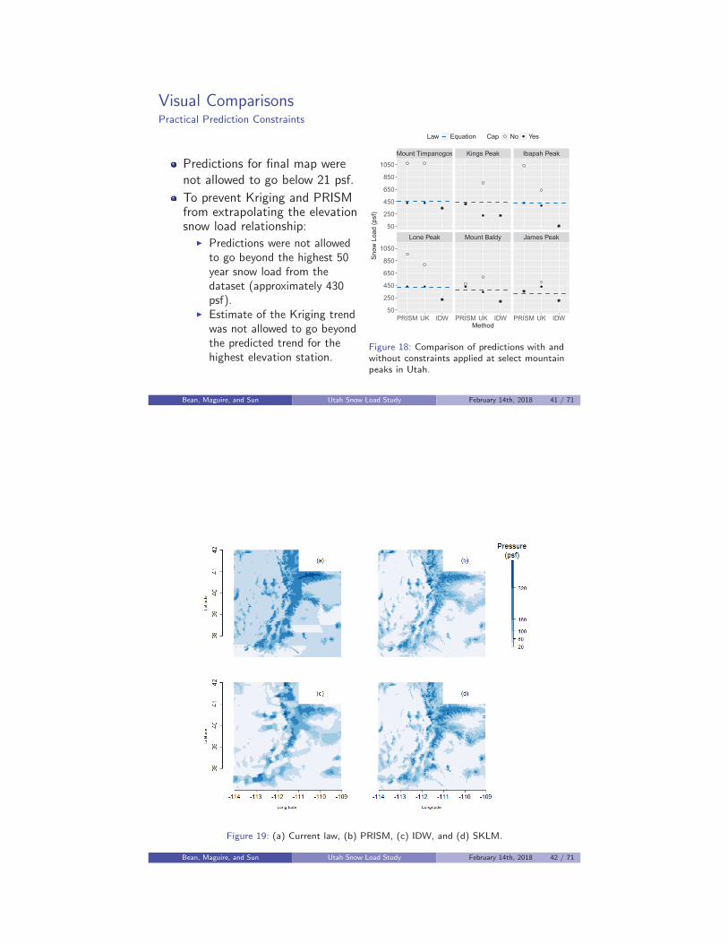
Visual ComparisonsPractical Prediction Constraints
Predictions for final map werenot allowed to go below 21 psf.
To prevent Kriging and PRISMfrom extrapolating the elevationsnow load relationship:
� Predictions were not allowedto go beyond the highest 50year snow load from thedataset (approximately 430psf).
� Estimate of the Kriging trendwas not allowed to go beyondthe predicted trend for thehighest elevation station.
Lone Peak Mount Baldy James Peak
Mount Timpanogos Kings Peak Ibapah Peak
PRISM UK IDW PRISM UK IDW PRISM UK IDW
50
250
450
650
850
1050
50
250
450
650
850
1050
Method
Snow
Loa
d (p
sf)
Law Equation Cap No Yes
Figure 18: Comparison of predictions with andwithout constraints applied at select mountainpeaks in Utah.
Bean, Maguire, and Sun Utah Snow Load Study February 14th, 2018 41 / 71
Figure 19: (a) Current law, (b) PRISM, (c) IDW, and (d) SKLM.
Bean, Maguire, and Sun Utah Snow Load Study February 14th, 2018 42 / 71
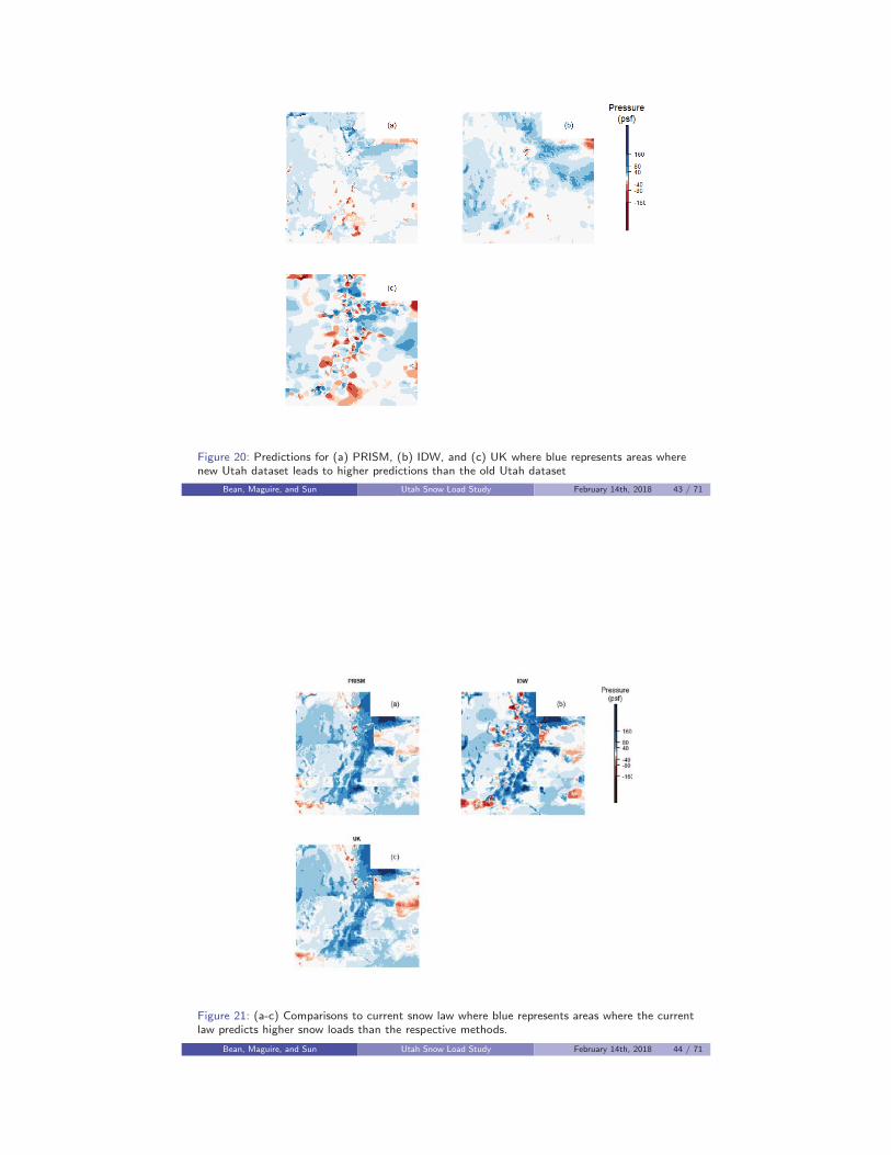
Figure 20: Predictions for (a) PRISM, (b) IDW, and (c) UK where blue represents areas wherenew Utah dataset leads to higher predictions than the old Utah dataset
Bean, Maguire, and Sun Utah Snow Load Study February 14th, 2018 43 / 71
Figure 21: (a-c) Comparisons to current snow law where blue represents areas where the currentlaw predicts higher snow loads than the respective methods.
Bean, Maguire, and Sun Utah Snow Load Study February 14th, 2018 44 / 71
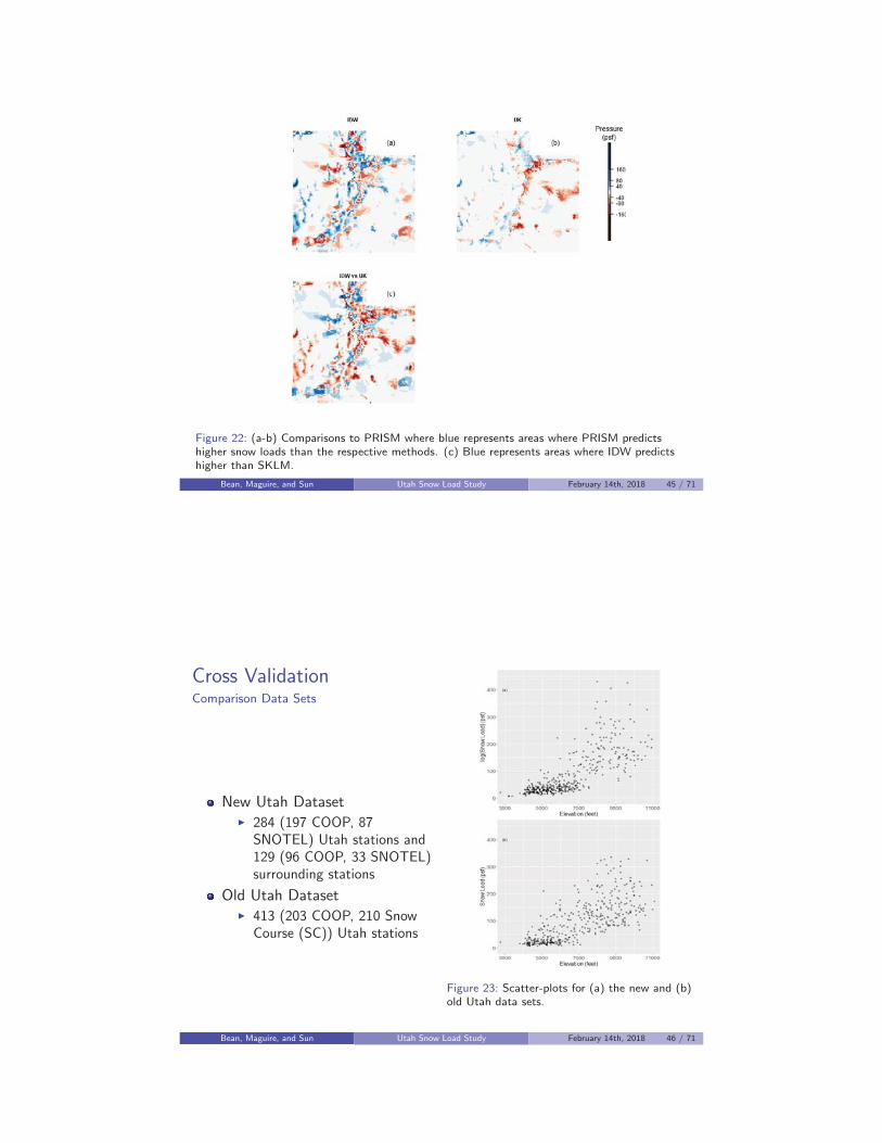
Figure 22: (a-b) Comparisons to PRISM where blue represents areas where PRISM predictshigher snow loads than the respective methods. (c) Blue represents areas where IDW predictshigher than SKLM.
Bean, Maguire, and Sun Utah Snow Load Study February 14th, 2018 45 / 71
Cross ValidationComparison Data Sets
New Utah Dataset� 284 (197 COOP, 87
SNOTEL) Utah stations and129 (96 COOP, 33 SNOTEL)surrounding stations
Old Utah Dataset� 413 (203 COOP, 210 Snow
Course (SC)) Utah stations
Figure 23: Scatter-plots for (a) the new and (b)old Utah data sets.
Bean, Maguire, and Sun Utah Snow Load Study February 14th, 2018 46 / 71
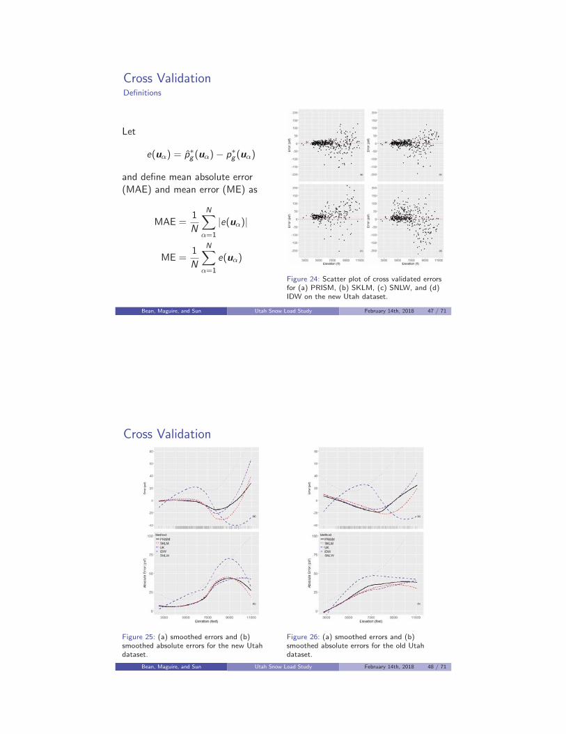
Cross ValidationDefinitions
Let
e(uα) = p∗g (uα)− p∗g (uα)
and define mean absolute error(MAE) and mean error (ME) as
MAE =1
N
N∑α=1
|e(uα)|
ME =1
N
N∑α=1
e(uα)
Figure 24: Scatter plot of cross validated errorsfor (a) PRISM, (b) SKLM, (c) SNLW, and (d)IDW on the new Utah dataset.
Bean, Maguire, and Sun Utah Snow Load Study February 14th, 2018 47 / 71
Cross Validation
Figure 25: (a) smoothed errors and (b)smoothed absolute errors for the new Utahdataset.
Figure 26: (a) smoothed errors and (b)smoothed absolute errors for the old Utahdataset.
Bean, Maguire, and Sun Utah Snow Load Study February 14th, 2018 48 / 71
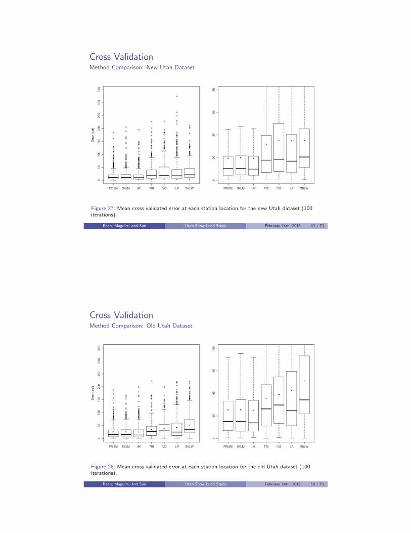
Cross ValidationMethod Comparison: New Utah Dataset
Figure 27: Mean cross validated error at each station location for the new Utah dataset (100iterations).
Bean, Maguire, and Sun Utah Snow Load Study February 14th, 2018 49 / 71
Cross ValidationMethod Comparison: Old Utah Dataset
Figure 28: Mean cross validated error at each station location for the old Utah dataset (100iterations).
Bean, Maguire, and Sun Utah Snow Load Study February 14th, 2018 50 / 71
Cross Validation
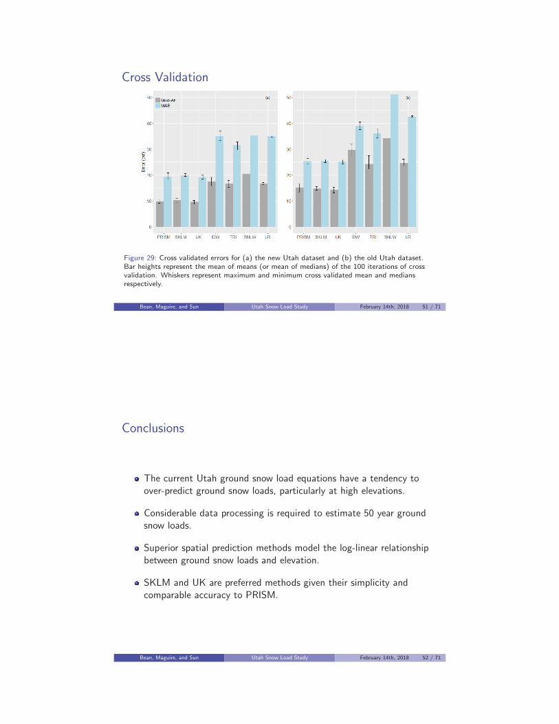
Figure 29: Cross validated errors for (a) the new Utah dataset and (b) the old Utah dataset.Bar heights represent the mean of means (or mean of medians) of the 100 iterations of crossvalidation. Whiskers represent maximum and minimum cross validated mean and mediansrespectively.
Bean, Maguire, and Sun Utah Snow Load Study February 14th, 2018 51 / 71
Conclusions
The current Utah ground snow load equations have a tendency toover-predict ground snow loads, particularly at high elevations.
Considerable data processing is required to estimate 50 year groundsnow loads.
Superior spatial prediction methods model the log-linear relationshipbetween ground snow loads and elevation.
SKLM and UK are preferred methods given their simplicity andcomparable accuracy to PRISM.
Bean, Maguire, and Sun Utah Snow Load Study February 14th, 2018 52 / 71
Applications
City by City Comparisons
Bean, Maguire, and Sun Utah Snow Load Study February 14th, 2018 53 / 71
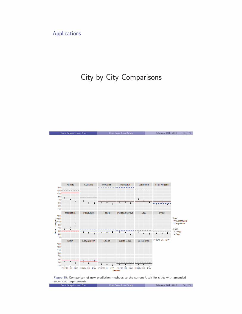
Figure 30: Comparison of new prediction methods to the current Utah for cities with amendedsnow load requirements.
Bean, Maguire, and Sun Utah Snow Load Study February 14th, 2018 54 / 71

Figure 31: Comparison of new prediction methods at northern county seats.
Bean, Maguire, and Sun Utah Snow Load Study February 14th, 2018 55 / 71
Figure 32: Comparison of new prediction methods at southern county seats.
Bean, Maguire, and Sun Utah Snow Load Study February 14th, 2018 56 / 71

Figure 33: Comparison of new prediction methods at locations where predictions are notablyhigher than current law.
Bean, Maguire, and Sun Utah Snow Load Study February 14th, 2018 57 / 71
Applications
County Specific Comparisons
Bean, Maguire, and Sun Utah Snow Load Study February 14th, 2018 58 / 71
Duchesne County
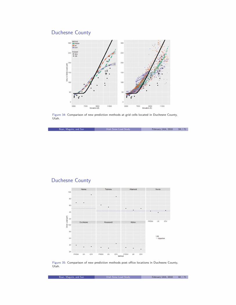
Figure 34: Comparison of new prediction methods at grid cells located in Duchesne County,Utah.
Bean, Maguire, and Sun Utah Snow Load Study February 14th, 2018 59 / 71
Duchesne County
Figure 35: Comparison of new prediction methods post office locations in Duchesne County,Utah.
Bean, Maguire, and Sun Utah Snow Load Study February 14th, 2018 60 / 71

Summit County
Figure 36: Comparison of new prediction methods at grid cells located in Summit County, Utah.
Bean, Maguire, and Sun Utah Snow Load Study February 14th, 2018 61 / 71
Summit County
Figure 37: Comparison of new prediction methods post office locations in Summit County, Utah.
Bean, Maguire, and Sun Utah Snow Load Study February 14th, 2018 62 / 71
Applications
Border Comparisons
Bean, Maguire, and Sun Utah Snow Load Study February 14th, 2018 63 / 71
Applications
0
50
100
150
200
250
300
350
Snow
Loa
d (p
sf)
PRISMIdahoUtah Minimum
0
50
100
150
200
250
300
350
−114 −113 −112 −111Degrees Longitude
Snow
Loa
d (p
sf)
UKIdahoUtah Minimum
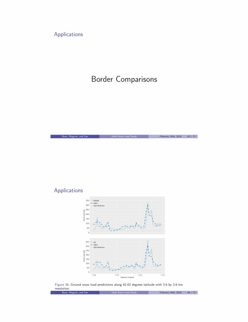
Figure 38: Ground snow load predictions along 42.02 degrees latitude with 3.6 by 3.6 kmresolution.
Bean, Maguire, and Sun Utah Snow Load Study February 14th, 2018 64 / 71
Applications
0
30
60
90
120
Snow
Loa
d (p
sf)
PRISMColoradoUtah Minimum
0
30
60
90
120
37 38 39 40 41Degrees Latitude
Snow
Loa
d (p
sf)
UKColoradoUtah Minimum
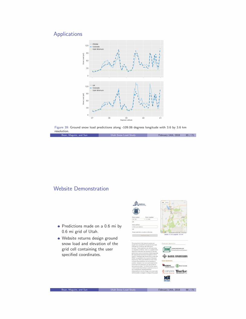
Figure 39: Ground snow load predictions along -109.06 degrees longitude with 3.6 by 3.6 kmresolution.
Bean, Maguire, and Sun Utah Snow Load Study February 14th, 2018 65 / 71
Website Demonstration
Predictions made on a 0.6 mi by0.6 mi grid of Utah.
Website returns design groundsnow load and elevation of thegrid cell containing the userspecified coordinates.
Bean, Maguire, and Sun Utah Snow Load Study February 14th, 2018 66 / 71
Thank YouIn addition to the SEAU, the authors would like to thank the followingsponsors.
Bean, Maguire, and Sun Utah Snow Load Study February 14th, 2018 67 / 71
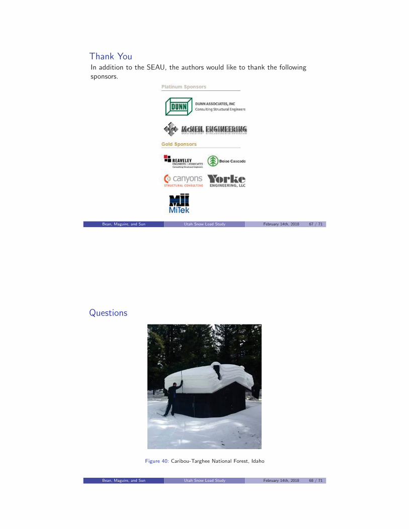
Questions
Figure 40: Caribou-Targhee National Forest, Idaho
Bean, Maguire, and Sun Utah Snow Load Study February 14th, 2018 68 / 71

References I
[1] Utah mapping portal. https://gis.utah.gov/.
[2] Christopher Daly, Wayne P Gibson, George H Taylor, Gregory L Johnson, andPhillip Pasteris. A knowledge-based approach to the statistical mapping of climate.Climate research, 22(2):99–113, 2002.
[3] Christopher Daly, Michael Halbleib, Joseph I. Smith, Wayne P. Gibson, Matthew K.Doggett, George H. Taylor, Jan Curtis, and Phillip P. Pasteris. Physiographicallysensitive mapping of climatological temperature and precipitation across theconterminous united states. International Journal of Climatology,28(15):2031–2064, 2008.
[4] Marie Laure Delignette-Muller and Christophe Dutang. fitdistrplus: An R packagefor fitting distributions. Journal of Statistical Software, 64(4):1–34, 2015.
[5] Pierre Goovaerts. Geostatistics for natural resources evaluation. Oxford UniversityPress, 1997.
[6] Pierre Goovaerts. Geostatistical approaches for incorporating elevation into thespatial interpolation of rainfall. Journal of hydrology, 228(1):113–129, 2000.
Bean, Maguire, and Sun Utah Snow Load Study February 14th, 2018 69 / 71
References II
[7] G. Matheron. The Theory of Regionalized Variables and its Applications. EcoleNationale Superieure des Mines de Paris, Paris, France, 1971.
[8] Jay Michaels. meteorologynews.com.
[9] Andrzej S Nowak and Kevin R Collins. Reliability of structures. CRC Press, 2012.
[10] Ronald L Sack, Richard J Nielsen, and Bruce R Godfrey. Evolving studies of groundsnow loads for several western us states. Journal of Structural Engineering, page04016187, 2016.
[11] Ronald L Sack and Azim Sheikh-Taheri. Ground and roof snow loads for Idaho.University of Idaho, Department of Civil Engineering, 1986.
[12] SEAU. Utah snow load study, 1992.
[13] Matthew Sturm, Brian Taras, Glen E. Liston, Chris Derksen, Tobias Jonas, and JonLea. Estimating snow water equivalent using snow depth data and climate classes.Journal of Hydrometeorology, 11(6):1380–1394, 2010.
[14] USGS. The national map. http://nationalmap.gov/, 2016.
Bean, Maguire, and Sun Utah Snow Load Study February 14th, 2018 70 / 71

References III
[15] USGS. Watershed boundary dataset. https://nhd.usgs.gov/wbd.html, 2016.
[16] Utah Water Science Center.https://ut.water.usgs.gov/infodata/basins.html.
Bean, Maguire, and Sun Utah Snow Load Study February 14th, 2018 71 / 71