Risk and Return models for Equity Markets and

Implied Equity Risk Premium

Enzo Busseti

May 19, 2010

Abstract

Equity risk premium is a central component of every risk and returnmodel in finance and a key input to estimate costs of equity and capitalin both corporate finance and valuation.

The article by Damodaran [1] examines three broad approachesfor estimating the equity risk premium. The first is survey based, itconsists in asking common investors or big players like pension fundmanagers what they require as a premium to invest in equity. Thesecond is to look at the premia earned historically by investing instocks, as opposed to riskfree investments. The third method triesto extrapolate a market-consensus on equity risk premium (ImpliedEquity Risk Premium) by analysing equity prices on the market today.

After having introduced some basic concepts and models, I’ll brieflyexplain the pluses and minuses of the first two methods, and analysemore deeply the third. In the end I’ll show the results of my estimationof ERP on real data, using variants of the Implied ERP (third) method.

1 Introduction

1.1 Equity Risk Premium

Risk aversion is a central notion in modern finance. Put in simple terms, in-vestors require higher returns for risky investments like stocks than safe oneslike Treasuries (Federal Reserve bills and bonds). The difference is called“risk premium”: it is the excess return expected from the risky investmentabove a risk-free return. In the case of stocks in general this difference iscalled the Equity Risk Premium. It refers to the perfomance of the overallmarket (in practice a broad market index like the S&P 500). There is vig-orous debate among experts about the method employed to calculate theequity premium and, of course, the resulting answer.A good estimate of equity risk premium is a key input in both corporatefinance evaluation and asset management. A firm invests in new assets andcapacity only if its managers think they can generate higher return than the

1

arX

iv:1

903.

0773

7v1

[q-

fin.

PR]

18

Mar

201

9

cost of the required capital. If equity risk premium increases, the cost ofraising capital increases, and thus we expect less investment in the overalleconomy.In asset management, equity risk premium is implicitly used when estimat-ing the expected return of the investments in stocks. This determines, forexample, the amount of money invested in the equity market by governmentsand corporations to meet future pension fund or healthcare obligations.In the following, we’ll keep it simple and sidestep a few technical issues. We’llwork with expected returns that are long-term, and pre-tax. By long-term,we mean something like 10 years, as short horizons raise questions of markettiming. (That is, it is understood that markets will be over or under-valuedin the short run.) Moreover, although individual investors should care aboutafter-tax returns, it is convenient to refer to pre-tax returns as do virtuallyall academic studies. Transaction costs and all other “market frictions” arealso neglected.

1.2 Portfolio Theory

In designing a portfolio, investors seek to maximize the expected return fromtheir investment, given some level of risk they are willing to accept. To afirst approximation, an asset’s return is modelled as a normally distributedrandom variable, and risk defined as its standard deviation.A portfolio is a weighted combination of assets, so that its return is theweighted combination of the returns of these assets. By combining differ-ent assets whose returns are not correlated, investors can reduce the totalvariance of the portfolio.Theoretically, if one could find sufficient securities with uncorrelated returns,he could reduce portfolio risk at any level he wants (by the Central LimitTheorem). Unfortunately, this situation is not typical in real financial mar-kets, where returns are positively correlated to a considerable degree becausethey tend to respond to the same set of influences. We can proceed further,and roughly simplify that set of influences to a single factor, to which stock’sreturn are correlated: the market return (as measured by a market indexlike S&P 500).Risk for individual stock returns is then split in two components: systematicand unsystematic risk. The first is the risk involving the whole market,and cannot be reduced through diversification. Business cycles, changes ininterest rate and wars all cause undiversifiable risks. Unsystematic risk isspecific to a single stock or group of stocks. It is not correlated with generalmarket movements: it can be for example a sudden strike by the employeesof a company or some technological innovation that moves value from onecompany (whose business becomes outdated) to another.To quantify the systematic risk of a stock we divide its return R in two parts:one perfectly correlated with and proportional to market return Rm, and a

2

second independent from the market (for simplicity a normally distributedvariable ε). Thus we have:

R = βRm + ε. (1)

The proportionality factor β is a market sensitivity index, indicating howsensitive the security is to changes in the market level. It is usually esti-mated by linear regression on historical data (security returns versus marketreturns). All ε from different stocks are uncorrelated (independent) by theabove assumption, the only source of correlation among stock returns is thegeneral market movement Rm. In addition, the ε mean sould be 0, as itrepresents random umpredictable events.Using this definition of security return (“market model”) the systematicrisk is β times the standard deviation of the market return σm, and theunsystematic risk is simply the std. dev. of the residual return factor σε.We can compute a portfolio’s βp factor as an average of the components’ βweighted by the proportion of each security. The portfolio’s systematic riskis in turn its βp factor times σm. Given the assumptions we made on ε, theCentral Limit Theorem assures that the portfolio’s unsystematic risk tendsinstead to 0 as the number of securities held in the portfolio grows.

1.3 Capital Asset Pricing Model

In the above section two measures of risk for a security have been devel-oped: the total risk (standard deviation of return) and the relative index ofundiversifiable risk β. In the capital asset pricing model (CAPM) only βis used to quantify risk, neglecting the portion of risk that is diversifiable.Securities with higher systematic risk should have higher expected returns.The basic postulate underlying CAPM theory is that assets with the samesystematic risk should have the same expected rate of return: that is, theprices of assets in the capital markets should adjust until equivalent riskassets have identical expected returns.Consider for example an investor who holds a risky portfolio with β = 1(same risk as the market portfolio): he should expect the same return asthat of the market portfolio. Another investor holding a riskless portfolio(β = 0) should instead expect the same rate of return of riskless assets, suchas Federal Reserve Treasury Bills.Now, consider the case of an investor who holds a mixture of these twoportfolios. The fraction of money allocated in the “market” portfolio equalsthe βp of the whole portfolio. We can also allow the investor to borrow atthe risk-free rate and invest the proceeds in the risky portfolio, so that theportofolio β becomes larger than 1.The expected return of the composite portfolio Rp is a weighted average ofthe expected returns on the two portfolios, one with risk-free return Rf and

3

the other with market return Rm:

E(Rp) = (1 − βp) Rf + βp E(Rm)

orE(Rp) = Rf + βp [E(Rm) −Rf ] (2)

We can rewrite this equation in term of risk premia, obtained subtractingthe risk-free rate from the rate of return. The portfolio risk premium andmarket risk premium (ERP) are given by:

rp = E(Rp) −Rf

rm = E(Rm) −Rf

Substituting into equation (2):

rp = βprm. (3)

In this form, CAPM states that the risk premium for a portfolio should beequal to the quantity of risk measured by its βp, times the market price forrisk, or Equity Risk Premium rp.

1.3.1 Beyond CAPM

As written above, one basic assumption of CAPM theory is that the onlyagent correlating different stock’s returns is the overall market movement.In this simplified picture a stock’s performance is linked to the surroundingeconomy only through its β factor, while it’s intuitively clear that manyother agents play important roles in determining a stock’s return. Vari-ous flavours of multifactor CAPM have been developed, basically extendingequation (1) to relate a stock’s return to many external factors:

R = β1F1 + β2F2 + · · · + βnFn + ε. (4)

The Fi can be chosen among macroeconomic indexes like unemployment, in-flation (or better surprises in inflation), interest rates, consumer confidence,etc. In practice every analyst chooses his own set of Fi factors, then a linearregression is used to estimate the βi. The next move is to assign a riskpremium ri to each factor Fi, and so we can write an equation analogous to(3) for the stock’s risk premium rs:

rs =

n∑i=1

βiri. (5)

It should be emphasized that while these models work well when dealingwith a single stock perfomance, the simple CAPM gives good estimate for

4

a broad market portfolio. The equity risk premium that appears in (3) isa market-wide number, affecting expected returns on all risky investments(the market price for risk). Using a larger equity risk premium will increasethe expected returns for all risky investments, and by extension, reduce theirprice.

1.4 Equity Risk Premium Determinants

Economic risk, or the health and predictability of the overall economy, is ofgreat importance. Put in simpler terms, the equity risk premium should belower in an economy with predictable inflation, interest rates and economicgrowth than in one where these variables are volatile.The risk aversion of investors in the markets is a critical factor in ERPevaluation. Higher risk aversion means higher risk premia, and lower equityprices, on the contrary as risk aversion declines, risk premia will fall. Itis the collective risk aversion of investors (across the whole market), thatinfluences equity risk premium. Different groups may have very differentrisk aversion profiles (for example it is understood that risk aversion growswith age).The relationship between information and equity risk premium is complex.More precise information should lead to lower risk premia, since it becomessimpler to forecast future earnings and cash flows. On the other hand, in gen-eral more informations (possibly unprecise) create more uncertainty aboutfuture earnings, since investors disagree about how best to interpret these. Inaddition, information differences may be one reason why investors demandlarger risk premia in some emerging markets than in others: markets varywidely in terms of transparency and information disclosure requirements.

2 Survey Based Evaluation

One method to evaluate equity risk premium is to ask investors what theyrequire as excess return from investments in stock over the risk free rate.Since there are millions of investors in the stock market, one challenge is tofind a representative subset. These are some of surveys used in practice.

• Individual investors are polled about their optimism for future stockprices, and their expected return on stocks. These polls are too muchsensible to recent stock price movements, showing higher investors’confidence after periods of price growth. Psychological effects play alsoan important role, as it seems that survey numbers vary depending onthe framing of the questions.

• Institutional investors and financial professionals are also surveyed.Some services track financial newletters and forums to estimate an

5

advisor sentiment index about the future direction of equities. Othersask the Chief Financial Officers (CFOs) of companies about their ex-pected equity risk premium. These surveys provide values which makemore sense than the indivduals’, but still they show too big standarddeviations to be taken seriously. Expected premia vary from 1.2% atthe first percentile to 12.4% at the tenth.

• Some surveys focus on academics, asking financial economists whatthey think is a good estimate of equity risk premium. The rationalehere is that economists’ opinion is highly influential to both students(who are the future managers) and practitioners, who read papers andbooks. As with the other survey estimates, there is a wide range ofopinion (too high standard deviation) and in general the values arehigher than those proposed by institutional investors.

This method shows therefore serious drawbacks: results vary wildly depend-ing on the set of investors or experts chosen, and even choosing restrictedsets of people with similar market influence and knowledge does not help.

3 Historical Premium Evaluation

This is probably the most widely used approach to estimate equity riskpremium: the returns earned on stocks over a long time period are estimated,and compared to the returns of a default-risk-free asset on the same timeperiod. Again there are large differences between the various estimates: hereare some reasons for these divergences.

• Different time periods used for estimation, i.e. how far back in timewe should go to estimate this premium (in the U.S. market data areavailable from ≈ 1870). Using shorter and recent time periods hasthe advantage of providing an up-to-date estimate, as investors’ andmarket features have changed much over the last century (even inmature markets like the U.S.). On the other hand a longer time periodmeans more points to average on, and therefore lower noise (standarddeviation) in the risk premium estimate. A good compromise mightbe to use an exponential weighted average that gives more weight torecent years, and progressively less to the points further back in time.

• There are many possible choices of risk-free rates. We can choose asrisk-free rate returns earned by every type of treasury security: short-term (treasury bills in the U.S.) or long term (treasury bonds). Thelogic choice here are the treasuries whose time to maturity is mostsimilar to the time horizon on which we are interested. For a medium-long term investment, if we want to avoid problems of market timing,a ten year treasury bond is a good choice.

6

• There are many possible way to measure equity returns, too. A naturalchoice is a popular market index (like Dow Jones), since its historicalvalues are more widely accessible and reliable than individual stocks’.It should be noted however, that if we are interested in the perfo-mance of the whole stock market we should measure returns on thebroadest possible portfolio (Dow Jones consists of only the 30 biggestcompanies) so other indices with shorter history, like S&P 500, may bebetter. A common error that can be caused by the choice of a narrowindex is the so called “survivor bias”, because companies which wentbankrupt are singled out from the index calculation: the returns maybe biased upwards.

• There is some debate about whether it’s better to use nominal returnsor real returns (adjusted for inflation). As long as equity risk premiumis concerned however, we should not bother: inflation rate would addto both risk-free and equity returns, so after taking the difference itvanishes.

• When computing the average risk premium on a given period, for ex-ample over 10 years starting from a series of returns for each quarter,we can opt for a geometric or an arithmetic average. This is an opendebate, a study by Indro and Lee [2] in 1997 concludes that both ap-proaches are biased (the arithmetic upwards, and the geometric down-wards). A well known inequality states that Marithmetic ≥Mgeometric,and the two are equal if and only if all returns averaged are equal.Being the returns very volatile, the difference between the results ofthe two averaging approaches can be substantial. Again, many practi-tionists use a compromise of the two, a weighted average of arithmeticand geometric mean (see [3]).

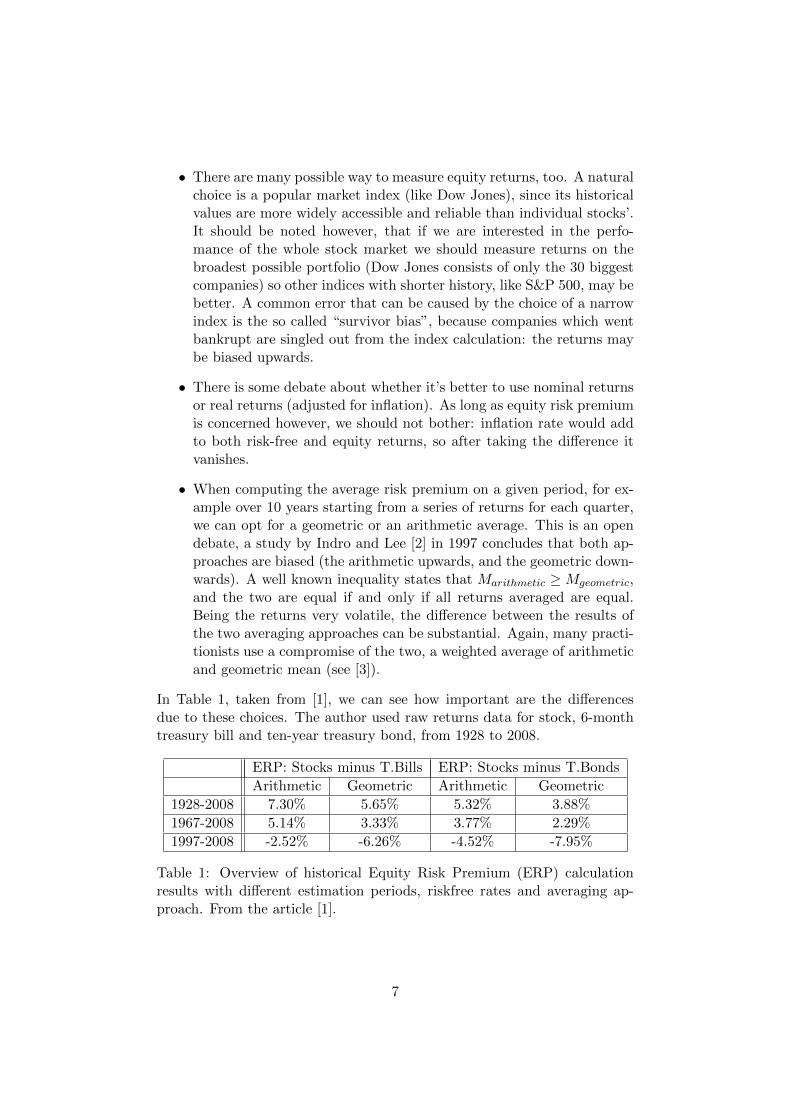
In Table 1, taken from [1], we can see how important are the differencesdue to these choices. The author used raw returns data for stock, 6-monthtreasury bill and ten-year treasury bond, from 1928 to 2008.

ERP: Stocks minus T.Bills ERP: Stocks minus T.Bonds

Arithmetic Geometric Arithmetic Geometric

1928-2008 7.30% 5.65% 5.32% 3.88%

1967-2008 5.14% 3.33% 3.77% 2.29%

1997-2008 -2.52% -6.26% -4.52% -7.95%

Table 1: Overview of historical Equity Risk Premium (ERP) calculationresults with different estimation periods, riskfree rates and averaging ap-proach. From the article [1].

7

4 Implied Equity Risk Premium

Another method widely used in estimates consists in extrapolating requiredrates of return from the market prices of equities. Then, subtracting today’srisk-free rates, we have an up-to-date estimate of equity risk premium.The idea is based on the basic concept that as investors price an assets,they are implicitly telling what they require as an expected return on it.Price is defined as the present value of all asset’s expected future cash flows(Discounted Cash Flow Model):

P =n∑i=0

CFi(r)i

(6)

where P is the price of the security now, CFi is the expected cash flow atthe end of period i, and r the required yield on each period.For an investment in equity the expected cash flows are dividends (one foreach period) and the money received at the end when selling back.

4.1 Dividend Based Approach (Gordon Model)

This model determines the fair value of a stock as the present value ofthe series of its dividend payments, assuming that dividends will grow at aconstant rate. In practice, the fair price P of a stock is a function of thedividend payed out today D, its expected growth rate g and the requiredrate of return k:

P =∞∑t=1

D × (1 + g)t

(1 + k)t=

D1

k − g(7)

where D1 = D(1 + g) is the dividend next period. Solving for k we obtain:

k =D1

P+ g

so in this model the required rate of return on a stock is simply its dividendyield plus the expected growth rate of its dividend payouts.This model assumes that the firm in evaluation will sustain constant growthforever. This is not an acceptable simplification in many practical cases:for example we should allow earnings to grow at extraordinary rates for theshort term, and then settle at the risk-free rate (as extrapolated from theterm structure of Fed. bonds interest rates). So we would split the sum inEq. (7) in different parts for the short and long term dividends/growth.

4.2 Earnings Based Approach

This is a slightly more refined variant of the dividend model, where we focuson earnings instead of dividends. We are addressing a flaw in the Gordon

8

Model, which assumes that companies pay out as much as they can affordto in dividends (and this is generally not true). We make some substitutionin Eq. (7):

• we replace D1 with the Earnings Per Share (EPS) times the payoutratio p (the fraction of earnings distributed in dividends);

• the expected growth rate of dividends g is substituted with the ex-pected rate of return k times the retention ratio (fraction of earningsreinvested, 1 − p). The rationale is that the growth of earnings is dueto the fraction of earnings reinvested, at a rate equal to the expectedrate k (of market consensus).

P =EPS · p

k − k · (1 − p)=EPS

k(8)

The inverse of the PE ratio (also referenced as the earnings yield) becomesthe required return on equity.This model too has the potential flaw of assuming constant growth of thestock. This assumption has two components: constant dividend payout ratioand constant return on investments. The former is not true in the long run,especially for younger firms who reinvest all earnings in the first “growth”years and then start paying dividends. The latter is also questionable, bothbecause growth rates change with time (a correction similar to that dis-cussed above may help), and because managers may not be able to investall earnings at the same rate k.

5 Analysis

I have used the last method described to extrapolate an implied equity riskpremium from the market value of the stocks’ prices. My goal is to see howthe formula (8), for the estimation of equity risk premium, behaves withdaily data.I worked with the S&P 500 index: from their site I got EPS estimation(weighted average for all firms composing the index) for each quarter, from1988 to 2009. I smoothed the data with an exponential moving average ofperiod 50 days (less than the sampling frequency of ≈ 100 days). The resultis shown in Figure 1.Then I downloaded the daily values of the index in those twenty years,reported in Figure 2.Finally I got from the site of the Federal Reserve daily quotations of bondsrates. In Figure 3 we have annual yields for 10 years bonds.The next step was to apply the formula (8) discussed above, and obtain itsestimation of Equity Risk Premium. The result is shown in Figure 4.The first striking result we notice is that the premium estimated in thisway is not always positive, there were two long periods (1989-1994 and

9

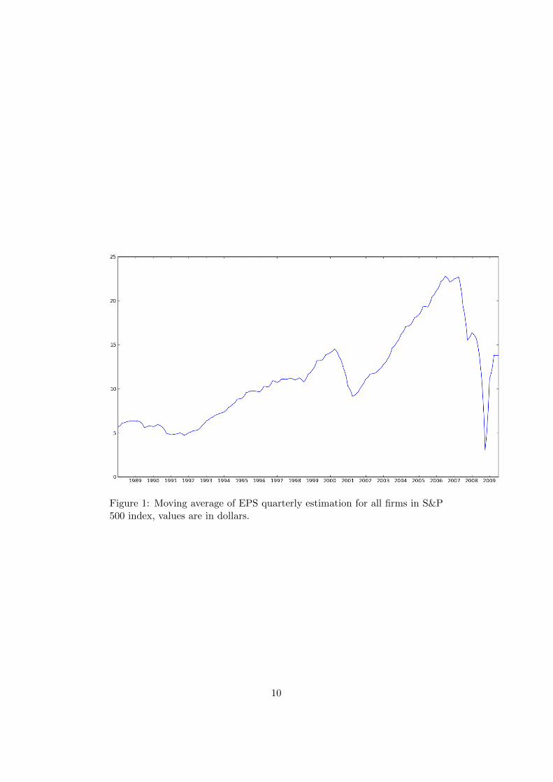
Figure 1: Moving average of EPS quarterly estimation for all firms in S&P500 index, values are in dollars.

10

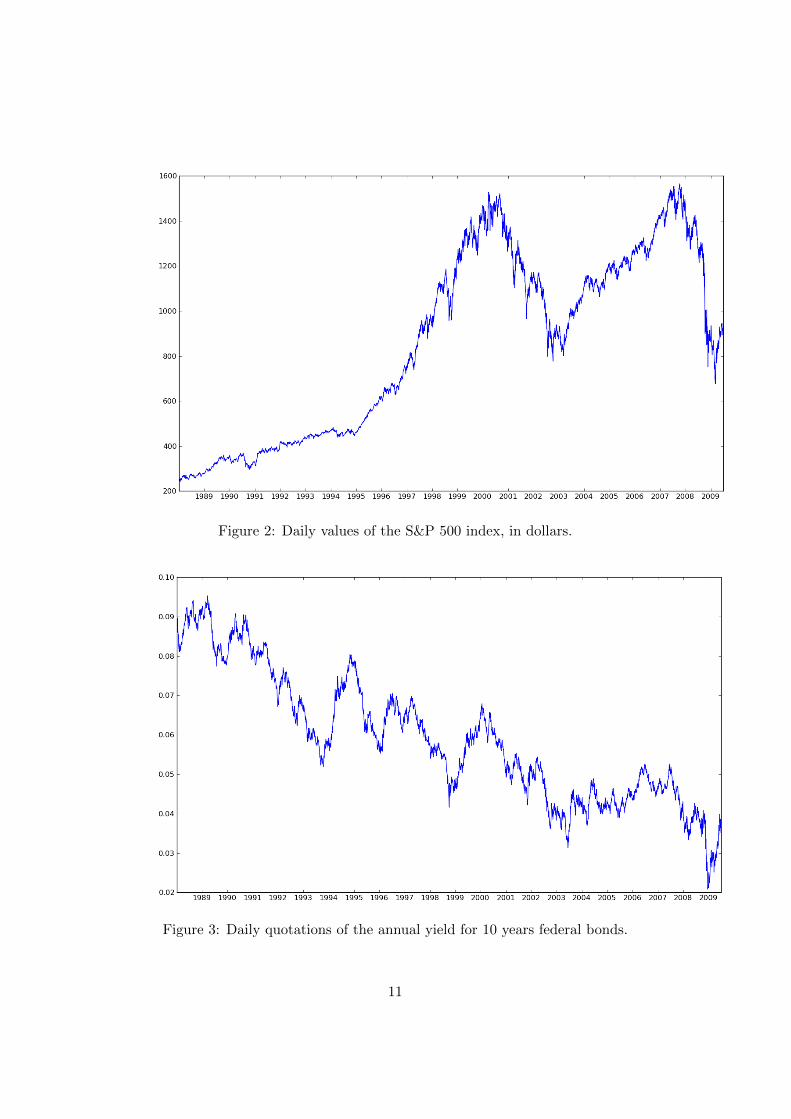
Figure 2: Daily values of the S&P 500 index, in dollars.

Figure 3: Daily quotations of the annual yield for 10 years federal bonds.

11

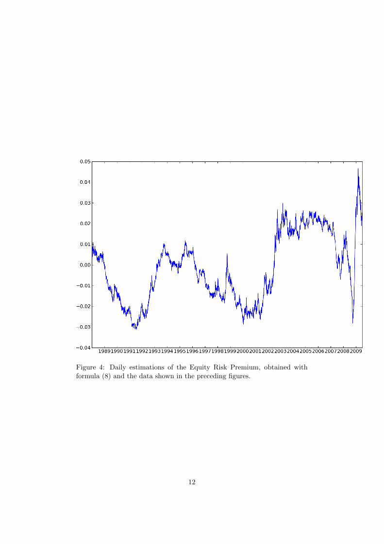
Figure 4: Daily estimations of the Equity Risk Premium, obtained withformula (8) and the data shown in the preceding figures.

12

1996-2002) when it went below zero. We can interpret these as investors’expectations of greater perfomance than a simple growth of earnings. Then,the 2008 crisis shows a sudden decrease in risk premium, as EPS went down,and then the expected big increase when prices fell.In general we can say that Eq. (8) is still too naıf to provide reliable resultover a wide range of data. There’s only a period (2003-2007) in which theresulting premium has meaningful and almost constant value, otherwise itoscillates with the movement of the underlying variables, showing that theremust be hidden complexity ignored by Eq. (8).

13

References

[1] A. Damodaran Equity Risk Premiums (ERP): Determinants, Esti-mation and Implications - A Post-Crisis Update Available at SSRN:http://ssrn.com/abstract=1492717, 2009

[2] D.C. Indro and W.Y. Lee, Biases In Arithmetic And Geometric AveragesAs Estimates Of Long-Run Expected Returns And Risk Premia FinancialManagement, 1997

[3] M.E. Blume, Unbiased Estimates Of Long-Run Expected Rates Of ReturnJournal of the American Statistical Association (September), 1974

[4] F.J. Fabozzi, F.P. Modigliani, F.J. Jones Foundations of Financial Mar-kets and Institutions Prentice Hall, 2009

14