robust model predictive control of cement mill circuits
TRANSCRIPT

Robust Model Predictive control of Cement Mill
circuits
A THESIS
submitted by
M GURUPRASATH
(Roll Number: clk 0603)
for the award of the degree
of
DOCTOR OF PHILOSOPHY
DEPARTMENT OF CHEMICAL ENGINEERING.
NATIONAL INSTITUTE OF TECHNOLOGY,
TIRUCHIRAPPALLI-620015
August 2011

THESIS CERTIFICATE
This is to certify that the thesis titled Robust Model Predictive control of
Cement Mill circuits, submitted by GuruPrasath, to the National Institute
of Technology, Tiruchirappalli, for the award of the degree of Doctor of Phi-
losophy, is a bonade record of the research work carried out by him under my
supervision. The contents of this thesis, in full or in parts, have not been submitted
to any other Institute or University for the award of any degree or diploma.
Tiruchirappalli- 620 015.Date:
M. ChidambaramResearch GuideDepartment of Chemical EngineeringNational Institute of TechnologyTiruchirappalli- 620 015. India

ACKNOWLEDGEMENTS
I would like to thank Prof. M. Chidambaram for his invaluable guidance and
suggestions. The timely completion of this thesis is due to his constant support,
boundless work and planning. Even though he was busy as Director he spent much
time with me for discussions. In the last few months of this thesis, even though,
he is in IIT, Madras, he guided me in completing the thesis in time. Organizing
things in a suitable time frame inspired me to nish many things well before time.
It's my privilege to work with him.
I would like to thank M/s. FLSmidth Private Limited for allowing me to use the
commercial simulation package CEMulator for conducting various experiments to
compare various controllers. Also I would like to thank M/s. UltraTech Cement,
Arakkonam for trusting me and allowing to test the controller online.
I would also like to thank my co-supervisor Dr. John Bagterp Jørgensen without
whom this Ph.D would not have been possible in its current form. Even though he
is busy in DTU, he is providing continuous support and guidance through online
discussions.
I would like to thank Prof. T. K. Radhakrishnan for his constant support during
initial phase of this PhD work and during the last few months of the thesis work.
His initiatives and suggestions inspired me in completing things well before time.
I would like to express my gratitude to Mr. T. R. Hari, Mr. Sudeep Sar and Mr.
Rajendra Bhargava of FLSmidth Private Limited, for their encouragement and
support during the complete research work. It has been privilege to work with
them as they not only provided nancial support but also motivated me in all
possible ways.
My great thanks to Bodil Recke, Jørgen Knudsen, Hassan Yazdi and Bo Frederik-
sen of FLSmidth A/S. who initiated the research contract and kept always open
i

to the ideas that we suggested.
I am extremely thankful to my doctoral committee members, Prof. B. Venkatra-
mani, Dr. SankaraNarayanan, and Prof. T. K. Radhakrishnan for their critical
comments and valuable suggestions in due course of time. Also I would like to
thank Prof. N. Anantharaman for his timely support in completing this research
work.
I thank all the sta members in the Chemical Engineering Department for their
help and Co-operation.
I have no words to thank my colleague and friends Kavitha Stanley, Sridhar. P,
Jose Pinto and Ajit Balaji the way encouraged and motivated me in all possible
ways particularly in doing experimental works in oce and plant.
Finally this work might not have been completed without support of my family.
It is impossible to put in words the way my mother and wife supported me in
completing my thesis in due course of time.
ii

ABSTRACT
KEYWORDS: MPC ; Cement Mill; Moving Horizon; constraints.
The present work considers the control of ball mill grinding circuits which are
characterized by non-linearities and disturbances. The disturbances are due to
large variations and heterogeneities in the feed material. Thus the models obtained
by simple tests on these mills are subject to large uncertainties which may result
in poor performance of conventional control solutions.
A regularized ℓ2-norm based nite impulse response (FIR) predictive controller
with input and input-rate constraints is developed. The estimator used is based
on a simple constant output disturbance lter. The FIR based regulator problem
is solved by convex quadratic program (QP) by converting the objective function
into a standard form. The QP is solved using an algorithm based on interior point
method. The model used here is single input- single output SOPDT with a zero
transfer function model. The performance of the predictive controller in the face
of plant-model mismatch is investigated by simulations.
In order to improve the performance of MPC, a moving horizon constrained reg-
ularized ℓ2 estimator based on impulse response models is developed. Here the
estimator is used to estimate the unknown disturbance by solving the optimization
problem. By using a SOPDT with a zero transfer function model, the performance
of the estimator with measurement noise is provided. Also the closed loop perfor-
mance of a MPC with moving horizon estimator with SISO system is investigated.
The predictive controller is equipped with soft output constraints that are used
to have robustness against plant-model mismatch. Soft output constraints are
the limits around the set point, where the errors are penalized minimum within a
dead band called soft limits and penalized heavily as soon as the error exceeds the
iii
band. By simulation rst with SISO system and then with 2 × 2 MIMO system,
the performance of the proposed controller and conventional predictive controller
is investigated. For MIMO system, the input vectors are Elevator Load, Fineness
and the output vectors are Feed rate, Separator speed. In case of plant-model
mismatch more than 50 %, the conventional MPC response become oscillatory,
whereas the soft MPC provides lesser variations in output resulting in much stable
response.
The Model Predictive Controller (MPC) with soft constraints is used for regula-
tion of a cement mill circuit. The uncertainties in the cement mill model are due to
heterogeneities in the feed material as well as operational variations. The uncer-
tainties are characterized by the gains, time constants, and time delays in a transfer
function model. The controllers are compared using a rigorous cement mill circuit
simulator. The simulations reveal that compared to conventional MPC, soft MPC
regulates cement mill circuits better by reducing the variations in manipulated
variables by 50%.
The performance of MPC with soft constraints is also compared with existing
Fuzzy Logic controller implemented in a real time plant with closed circuit ce-
ment ball mill. The real time results show that the standard deviation of manip-
ulated variables and the controlled variables are reduced with the soft MPC. The
reduction in standard deviation in quality is 23%.
The performance of the same controller (MPC) applied to a cement ball milling
circuit with large measurement sample delay is investigated. Usually neness is
measured hourly by sample analysis in the laboratory. The predictive controller
designed with the model from fast sample data (1 min sample) when applied to
control with hourly sampled measurements, the controller is to be re-tuned. The
parameters needed to be re-tuned are weight for penalties on measurement error
(Qz), weights of penalties on manipulated variables (S) and rate of change of
manipulated variables (R). Also the hard constraints on input- rate movements
are to be re-tuned to reduce the variations in the controller. In this work, the
controller model is added with half the sample delay of measurement to improve
the performance of the controller with one time tuning.
iv

TABLE OF CONTENTS
ACKNOWLEDGEMENTS i
ABSTRACT iii
LIST OF TABLES ix
LIST OF FIGURES xiii
ABBREVIATIONS xiv
NOTATION xv
1 Introduction 1
1.1 Motivation . . . . . . . . . . . . . . . . . . . . . . . . . . . . . . 3
1.2 Objectives . . . . . . . . . . . . . . . . . . . . . . . . . . . . . . 5
2 Literature Survey 7
2.1 Model Predictive Control in Industries . . . . . . . . . . . . . . 7
2.2 Model Predictive Control . . . . . . . . . . . . . . . . . . . . . . 9
2.2.1 Elements of MPC . . . . . . . . . . . . . . . . . . . . . . 10
2.2.2 Dynamic Matrix Control . . . . . . . . . . . . . . . . . . 12
2.2.3 DMC tuning strategy . . . . . . . . . . . . . . . . . . . . 14
2.2.4 Principle of moving horizon MPC . . . . . . . . . . . . . 15
2.3 Review of MPC in industries . . . . . . . . . . . . . . . . . . . . 17
2.3.1 Review on Tuning of MPC . . . . . . . . . . . . . . . . . 22
2.3.2 MPC with Hard constraints . . . . . . . . . . . . . . . . 23
2.3.3 Soft Constrained MPC . . . . . . . . . . . . . . . . . . . 27
2.3.4 Robust Model Predictive controllers . . . . . . . . . . . . 33
2.4 Ball Mill Control . . . . . . . . . . . . . . . . . . . . . . . . . . 36
v

2.4.1 Cement Mill modeling . . . . . . . . . . . . . . . . . . . 41
2.5 Fuzzy Logic Controller in Cement Industries . . . . . . . . . . . 42
3 An evaluation of existing MPC tools 44
3.1 Introduction . . . . . . . . . . . . . . . . . . . . . . . . . . . . . 44
3.2 Dynamic Matrix Control(DMC) . . . . . . . . . . . . . . . . . . 47
3.3 FIR Model Based MPC . . . . . . . . . . . . . . . . . . . . . . . 50
3.3.1 Plant and Sensors . . . . . . . . . . . . . . . . . . . . . . 51
3.3.2 Regulator . . . . . . . . . . . . . . . . . . . . . . . . . . 52
3.3.3 Simple Estimator . . . . . . . . . . . . . . . . . . . . . . 53
3.4 Eect of Parameter Uncertainty in the System . . . . . . . . . . 54
3.4.1 Eect of Uncertainty in Gain . . . . . . . . . . . . . . . 55
3.4.2 Eect of Uncertainty in Time Constant . . . . . . . . . . 57
3.4.3 Eect of Uncertainty in zero β . . . . . . . . . . . . . . 58
3.4.4 Eect of Uncertainty in Time Delay . . . . . . . . . . . . 58
3.4.5 Eect of Measurement Noise and Process Noise . . . . . 60
3.5 Moving Horizon Estimation . . . . . . . . . . . . . . . . . . . . 64
3.5.1 Model used by Regulator and Estimator . . . . . . . . . 64
3.5.2 Regulator . . . . . . . . . . . . . . . . . . . . . . . . . . 65
3.6 Simulation . . . . . . . . . . . . . . . . . . . . . . . . . . . . . . 66
3.7 Soft Constrained MPC . . . . . . . . . . . . . . . . . . . . . . . 73
3.7.1 Soft Constraint Principle . . . . . . . . . . . . . . . . . . 74
3.7.2 Selection of Soft Limits . . . . . . . . . . . . . . . . . . . 76
3.8 Conclusion . . . . . . . . . . . . . . . . . . . . . . . . . . . . . . 77
4 Comparison of Soft MPC with Nominal MPC Using Simula-tion 79
4.1 Introduction . . . . . . . . . . . . . . . . . . . . . . . . . . . . . 79
4.2 Simulation . . . . . . . . . . . . . . . . . . . . . . . . . . . . . . 80
4.3 Soft constraints in MPC . . . . . . . . . . . . . . . . . . . . . . 81
4.3.1 Eect of including noise in the system . . . . . . . . . . 81
4.4 Eect of uncertainties in the model . . . . . . . . . . . . . . . . 82
vi

4.4.1 Eect of uncertainty in Delay . . . . . . . . . . . . . . . 83
4.4.2 Eect of uncertainty in gain . . . . . . . . . . . . . . . . 84
4.4.3 Eect of uncertainty in Time Constant . . . . . . . . . . 85
4.4.4 Eect of uncertainty in Zero . . . . . . . . . . . . . . . . 86
4.5 Eect of Process noise and Measurement noise . . . . . . . . . . 87
4.6 Simulation of MIMO System . . . . . . . . . . . . . . . . . . . . 88
4.6.1 Eect of uncertainty in gain . . . . . . . . . . . . . . . . 91
4.7 Conclusion . . . . . . . . . . . . . . . . . . . . . . . . . . . . . . 92
5 Cement Manufacturing Process 93
5.1 Introduction . . . . . . . . . . . . . . . . . . . . . . . . . . . . . 93
5.2 Cement Ball Mill Process . . . . . . . . . . . . . . . . . . . . . . 97
5.2.1 Tromp Curves . . . . . . . . . . . . . . . . . . . . . . . . 98
5.3 Cement Mill Control Strategy . . . . . . . . . . . . . . . . . . . 99
5.4 Cement Mill Model . . . . . . . . . . . . . . . . . . . . . . . . . 100
5.4.1 Step Test Procedure . . . . . . . . . . . . . . . . . . . . 101
5.5 Conclusion . . . . . . . . . . . . . . . . . . . . . . . . . . . . . . 105
6 Applications of Soft MPC to Cement Mill Circuit 106
6.1 Introduction . . . . . . . . . . . . . . . . . . . . . . . . . . . . . 106
6.2 Cement Mill control Simulation results . . . . . . . . . . . . . . 107
6.3 Real Time implementation . . . . . . . . . . . . . . . . . . . . . 112
6.4 Conclusion . . . . . . . . . . . . . . . . . . . . . . . . . . . . . . 118
7 Implementation of Soft MPC to a Large Sample Delay System 119
7.1 Introduction . . . . . . . . . . . . . . . . . . . . . . . . . . . . . 119
7.2 System Implementation . . . . . . . . . . . . . . . . . . . . . . . 121
7.3 Conclusion . . . . . . . . . . . . . . . . . . . . . . . . . . . . . . 124
8 Summary and Conclusions 126
8.1 An evaluation of existing MPC tools . . . . . . . . . . . . . . . 126
8.2 Comparison of soft MPC with conventional MPC . . . . . . . . 127
8.3 Application of Soft MPC in cement mill circuit . . . . . . . . . 127
vii

8.4 Implementation of Soft MPC to a Large Sample Delay System . 128
8.5 Conclusions . . . . . . . . . . . . . . . . . . . . . . . . . . . . . 129
A Quadratic Program Formulation 132
A.1 Quadratic program for FIR based MPC . . . . . . . . . . . . . . 132
A.2 Quadratic Program formulation for Estimator . . . . . . . . . . 134
A.3 Quadratic Program formulation for Soft MPC . . . . . . . . . . 138
B Flow Diagram for MPC Design 143
C General Form of Quadratic Program 144
C.1 Quadratic Program Formulation . . . . . . . . . . . . . . . . . . 144
D Interior Point Method Algorithm 147
D.1 Interior Point Method Algorithm . . . . . . . . . . . . . . . . . 147
E Matlab Program for Soft MPC design 152
E.1 Initialization of MPC . . . . . . . . . . . . . . . . . . . . . . . . 152
E.2 Soft MPC . . . . . . . . . . . . . . . . . . . . . . . . . . . . . . 158
E.3 MPC Design . . . . . . . . . . . . . . . . . . . . . . . . . . . . . 159
E.4 Closed Loop Simulation . . . . . . . . . . . . . . . . . . . . . . 161
F CEMulator 163
F.1 Application . . . . . . . . . . . . . . . . . . . . . . . . . . . . . 163
F.1.1 Background . . . . . . . . . . . . . . . . . . . . . . . . . 163
F.1.2 Benets . . . . . . . . . . . . . . . . . . . . . . . . . . . 164
F.1.3 Limitations . . . . . . . . . . . . . . . . . . . . . . . . . 164

LIST OF TABLES
2.1 Review of Model Predictive Control in industries. . . . . . . . . 21
2.2 Reported work on design and implementation of MPC with hardconstraints. . . . . . . . . . . . . . . . . . . . . . . . . . . . . . 26
2.3 Reported work on design of soft constraint based MPC. . . . . . 31
2.4 Reported work on MPC based on Second Order Cone ProgrammingTechnique . . . . . . . . . . . . . . . . . . . . . . . . . . . . . . 35
2.5 Reported work on MPC for ball milling processes . . . . . . . . 39
5.1 Cement Plant Variables . . . . . . . . . . . . . . . . . . . . . . 105
7.1 Comparison of Conventional control and Controller with sampleDelay. . . . . . . . . . . . . . . . . . . . . . . . . . . . . . . . . 125
ix

LIST OF FIGURES
2.1 Model Predictive Control Scheme. . . . . . . . . . . . . . . . . . 9
2.2 Generic model predictive control system. . . . . . . . . . . . . . 15
2.3 Principle of Moving Horizon MPC. . . . . . . . . . . . . . . . . 16
2.4 Penalty function and modied penalty function of Range control,yL = −1 yH = 1 . . . . . . . . . . . . . . . . . . . . . . . . . . . 29
3.1 Performance of Dynamic Matrix controller for step responses withdierent control weights λ = 0.1, 1, 10, 100, 1000. . . . . . . . . . 48
3.2 Performance of the DMC with uncertainty in delay with controlweight λ = 10. . . . . . . . . . . . . . . . . . . . . . . . . . . . 49
3.3 The principle of moving horizon estimation and control. . . . . . 53
3.4 Disturbance used for the simulations. . . . . . . . . . . . . . . . 55
3.5 Impulse responses for dierent gains, K, in (3.19a). . . . . . . . 56
3.6 Closed-loop MPC performance with gain uncertainty. . . . . . . 56
3.7 Impulse responses for dierent time constants, τ1, in Equation 3.19a. 57
3.8 Closed-Loop performance with uncertainty in one of the time con-stants, τ1. . . . . . . . . . . . . . . . . . . . . . . . . . . . . . . 57
3.9 Impulse responses for dierent values of β in (3.19a). . . . . . . 58
3.10 Closed-loop MPC response for uncertain values of zero β in theplant (3.19a). . . . . . . . . . . . . . . . . . . . . . . . . . . . . 59
3.11 Impulse responses for dierent time delays, τ , in Equation 3.19a. 59
3.12 Closed-loop MPC performance for uncertainties in plant time de-lays. . . . . . . . . . . . . . . . . . . . . . . . . . . . . . . . . . 60
3.13 Top: Deterministic disturbance function(D) with added processnoise. Bottom: Measurement noise(v). . . . . . . . . . . . . . . 60
3.14 Closed-loop MPC performance for the nominal system - StochasticCase, Top: Output with noise (blue) and Filtered value of out-put(green). . . . . . . . . . . . . . . . . . . . . . . . . . . . . . 61
3.15 Closed-loop MPC performance with plant gain K = 1.5 comparedto nominal gain K = 1.0 with noise included in the process, Top:Output with noise (blue) and Filtered value of output (green). . 61
x

3.16 Closed-loop MPC performance for τ1 = 6.5 with noise included inthe process (nominal value τ1 = 5), Top: Output with noise (blue)and Filtered value of output (green). . . . . . . . . . . . . . . . 62
3.17 Closed-loop MPC performance for β = 4 with noise included in theprocess (nominal value β = 2), Top: Output with noise (blue) andFiltered value of output (green). . . . . . . . . . . . . . . . . . . 62
3.18 Closed-loop MPC performance for uncertainty in delay τd = 7 withnoise included in the process. . . . . . . . . . . . . . . . . . . . 63
3.19 Moving horizon estimation and regulation. . . . . . . . . . . . . 64
3.20 Batch estimation with no measurement noise. Top: Measured Out-put Bottom: Actual and Estimated disturbance Low regularizationweights (Sd = 0.1 and Rw = 0.01). . . . . . . . . . . . . . . . . . 68
3.21 Batch estimation with measurement noise and (Sd = 0.1 , Rw =0.01). Top: Measured Output Z (solid line)and Output with noise Y(Dots). Bottom: Actual Disturbance (Dotted lines), the estimateddeterministic disturbance(blue) and the total disturbance(with thestochastic component added)(green). . . . . . . . . . . . . . . . 68
3.22 Batch estimation with measurement noise. Medium regularizationweights (Sd = 1 and Rw = 0.1), (Legends : As in Figure 3.21). . 69
3.23 Batch estimation with measurement noise. High regularizationweights (Sd = 5 and Rw = 0.5), (Legends : As in Figure 3.21). . 69
3.24 Moving Horizon Estimation with measurement noise (r = 0.2) and(Sd = 1 and Rw = 0.1), (Legends : As in Figure 3.21) . . . . . . 70
3.25 Closed-loop MPC simulation without measurement noise. Bottom:Actual disturbance (red dotted line) and the estimated disturbance(blue). Regularization (Sd = 0.1 and Rw = 0.01). . . . . . . . . 71
3.26 Closed-loop MPC simulation with measurement noise (r = 0.2).Low regularization (Sd = 0.1 and Rw = 0.01), Legends as in Figure3.25. . . . . . . . . . . . . . . . . . . . . . . . . . . . . . . . . . 72
3.27 Closed-loop MPC simulation with measurement noise (r = 0.2).Medium regularization (Sd = 1 and Rw = 0.1), Legends as in Figure3.25. . . . . . . . . . . . . . . . . . . . . . . . . . . . . . . . . . 72
3.28 Closed-loop MPC simulation with measurement noise (r = 0.2).High regularization (Sd = 5 and Rw = 0.5), Legends as in Figure3.25. . . . . . . . . . . . . . . . . . . . . . . . . . . . . . . . . . 73
3.29 The principle of soft constraint MPC and conventional MPC(Error,eVs Penalty Function, ρ). . . . . . . . . . . . . . . . . . . . . . . 75
3.30 Linear (green) and Quadratic term (pink) of the soft constraint. 77
xi

4.1 External signals used in simulation: Disturbance (dk) measurementnoise (v) and process noise(w). . . . . . . . . . . . . . . . . . . . 81
4.2 Comparison of Open loop performance of conventional and softMPC,with nominal models applied to a stochastic system with nodeterministic disturbance (Conventional MPC = blue, Soft MPC =red). . . . . . . . . . . . . . . . . . . . . . . . . . . . . . . . . . 82
4.3 Closed-loop MPC performance with uncertainty in time delay, τd =3, in Equation (4.2a)(Conventional MPC = blue, Soft MPC = red). 83
4.4 Closed-loop MPC performance with higher plant time delay , τd =7, in Equation (4.2a)(Conventional MPC = blue, Soft MPC = red). 84
4.5 Closed-loop MPC performance with gain uncertainty, K = 2, inEquation (4.2a)(Conventional MPC = blue, Soft MPC = red). . 85
4.6 Closed-loop MPC performance with uncertain time constant, τ1, inEquation (4.2a)(Conventional MPC = blue, Soft MPC = red). . 85
4.7 Closed-loop MPC performance with uncertain zero, β, in Equation(4.2a)(Conventional MPC = blue, Soft MPC = red). . . . . . . 86
4.8 Comparison of normal and soft MPC with nominal models appliedto a stochastic system with an unknown deterministic disturbance(Conventional MPC = blue, Soft MPC = red). . . . . . . . . . . 88
4.9 Closed-loop MPC performance with noise and gain uncertainty, Theplant gain isK = 2 and the model gain isK = 1(Conventional MPC= blue, Soft MPC = red). . . . . . . . . . . . . . . . . . . . . . 88
4.10 Disturbance Model as in Equation (4.5) with no process noise andmeasurement noise. . . . . . . . . . . . . . . . . . . . . . . . . . 90
4.11 Variation of controllers Nominal Case, as in Equation (4.4) (Con-ventional MPC = blue, Soft MPC = red). . . . . . . . . . . . . 91
4.12 Comparison of Conventional MPC and Soft MPC in case of Uncer-tainty in Gain, K (MIMO), in Equation (4.4)(Conventional MPC= blue, Soft MPC = red). . . . . . . . . . . . . . . . . . . . . . 92
5.1 Cement plant (FLSmidthA/S (2004)). . . . . . . . . . . . . . . . 94
5.2 Cement mill grinding circuit (FLSmidthA/S (2004)). . . . . . . 97
5.3 Ball mill(FLSmidthA/S (2004)). . . . . . . . . . . . . . . . . . . 98
5.4 Classier(FLSmidthA/S (2004)). . . . . . . . . . . . . . . . . . 99
5.5 Tromp Curve(FLSmidthA/S (2004)). . . . . . . . . . . . . . . . 100
5.6 Step Response results for dierent operating conditions(dierentGrindability factors ) and with dierent step sizes of Feed(+5 %,-5 % ..). . . . . . . . . . . . . . . . . . . . . . . . . . . . . . . . 102
xii

5.7 Step Response results for dierent operating conditions(dierentGrindability factors ) and with dierent step sizes of Separator(+5%, -5 % ..). . . . . . . . . . . . . . . . . . . . . . . . . . . . . . 103
5.8 Model identication based on the plots obtained from the step re-sponse co-ecient(CEMulator data). . . . . . . . . . . . . . . . 104
6.1 Performance of MPC with grindability factor of 36 without mea-surement noise(Sepax Power Changed from 330-360 Kw - Greenline). . . . . . . . . . . . . . . . . . . . . . . . . . . . . . . . . . 108
6.2 Performance of MPC with grindability factor of 28 and sepax powerchanged from 390- 300 KW(Green Line). . . . . . . . . . . . . 110
6.3 Conventional MPC(left) and Soft MPC(right) applied to a rigorousnonlinear cement mill simulator. The disturbances (change in hard-ness of the cement clinker) are introduced at time 1.35 hour (greenline) and the controllers are switched on at time 2 hour (purple line)The soft constraints are indicated by the dashed lines. . . . . . . 111
6.4 Model identication from the plant data from step response tests.The identied model is yellow solid line. The other lines indicateplot of real time data with various step tests conducted. The yellowline is based on the identication of the model with the other dataplotted. . . . . . . . . . . . . . . . . . . . . . . . . . . . . . . . 115
6.5 Comparison of Soft MPC (left) with the High Level controller (right)implemented in a closed loop cement mill Target (Red), Actualvalue (Blue), High and Low Limits(dashed line). . . . . . . . . 116
6.6 Actuator (left) and measurement (right) variations in soft MPCwhen the control parameters are inside and outside the soft con-straint limits (dotted lines) when made online with the cement millrecipe changed to OPC (pink line)(Real Time Results). . . . . 117
7.1 Operator station of High Level Control for closed loop cement millFLSmidthA/S (2004). . . . . . . . . . . . . . . . . . . . . . . . 121
7.2 Variations in MPC with nominal models when applied to measure-ments having large sample delays, Target(Red), Actual Value(Blue). 123
7.3 Variations in MPC with models including sample delay added tocontinuous model and taken online for controlling the large sampledelay parameters(Fineness), Target(Red), Actual Value(Blue). . 123
B.1 Program Flow for MPC Design . . . . . . . . . . . . . . . . . . 143
xiii

ABBREVIATIONS
NITT National Institute of Technology, Tiruchchirappalli
MPC Model Predictive Control
MHE Moving Horizon Estimation
MV Manipulated Variable
CV Controlled Variable
OPC Ordinary Portland Cement
PPC Puzzalona Portland Cement
SISO Single Input- Single Output
MIMO Multi Input - Multi Output
FOPDT First Order Plus Dead Time
SOPDT Second Order Plus Dead Time
xiv

NOTATION
A System matrixB Input matrixBd Input disturbance matrixdk Disturbance vectoryk Outputwk Process noisevk Measurement noiseuk Inputbk Bias EstimateP0, Q Variance of Process noiseR Variance of measurement noiseHi Impulse response coecientsH Hessian matrixg gradientQz Weight on measurement errorS Weight on Actuator movementsN Prediction Horizonn Control Horizonϕ Objective Functionη Soft constraintSη Weight on Soft constraintβ Zero of the systemτ1, τ2 Time constantsτd Time Delay
xv

CHAPTER 1
Introduction
Model predictive control (MPC) has become a standard technology in the high
level control of chemical processes. MPC or receding horizon control is a form of
control in which the control action is obtained by solving on-line, at each sampling
instant, a nite open-loop optimal control problem, using the current state of the
plant as the initial state; the optimization yields an optimal control sequence in
which the rst control move is applied to the plant.
However, only very little guidelines are available regarding tuning methodologies
of such controllers in the face of the inevitable plant-model mismatch. The closed-
loop performance of nominal linear model predictive control can be quite poor
when the models are uncertain. Consequently, some years after commissioning,
many high-level control systems are turned o due to poor closed-loop perfor-
mance. This is often due to changes in the plant dynamics caused by wear and
tear combined with lack of the necessary human resources at the plant to re-tune
and maintain the MPC.
Using soft output constraints along with hard constraints in a novel way, the poor
performance of predictive control in the case of plant-model mismatch can be im-
proved signicantly. Constraints are physical limitations the control system must
take into consideration when implementing control actions. Usually constraints
to the controllers are of two types, hard constraints and soft constraints. Hard
constraints are those which are need to be necessarily satised, whereas soft con-
straints can be violated but penalized heavily whenever violated. A constrained
optimization problem is one in which there are inequality or equality constraints
that are imposed while seeking to maximize an objective function.
Alternatively, a constrained optimization problem can be dened as a regular
constraint satisfaction problem augmented with a number of "local" cost functions.
1

The aim of constrained optimization is to nd a solution to the problem whose
cost, evaluated as the sum of the cost functions, is minimized. Excellent review on
Model predictive control and optimization methods are available on Maciejowski
(2002), Camacho and Bordons (2004) and Rossiter (2003).
The cement mill circuit requires many soft output constraints to be considered
in a MPC formulation of the control problem. It is one of the best examples of
highly non-linear system to be controlled by a linear model. The uncertainties in
the system are large enough to cause the plant-model mismatch quite often.
Further, Comminution is a major unit operation in a cement plant, accounting
for about 50 - 75 % of the total plant energy consumption. Comminution can
be of two types, ball mill grinding and vertical roller mill grinding. Nevertheless
when grinding is required the ball mill is the most accepted element in the cement
grinding. The reasons are high reliability, the good possibility of gypsum dehy-
dration, simple operation (does not necessarily mean ecient) and the easy to
maintain construction. Finish grinding based on ball mill operation in general is
extremely inecient. Just 4 % of energy available is eciently used for grinding.
Loading the cement mill too little results in early wear of the steel balls and a very
high energy consumption per tonnes cement produced. Conversely, loading the
mill too much results in inecient grinding such that the product quality cannot
be met. Cement quality is measured by its chemical composition and its particle
size distribution. Blaine is an aggregate number for the particle size distribution
measuring the specic surface area of the cement powder.
Loading the cement mill too much, may even result in a phenomena called plugging
such that the plant must be stopped and plugged material removed from the mill.
Consequently, optimization and control of their operation are very important for
running the cement plant eciently, i.e. minimizing the specic power consump-
tion and delivering consistent product quality meeting specications. New control
methodologies are proposed for improving the performance of such process. The
improved operation resulting from these controllers can potentially lead to large
energy savings and at the same time provide a more consistent product quality.
2

1.1 Motivation
Extensive research is being conducted for improving the performance of dierent
modules in the cement process. The control of ball mill grinding circuit is con-
sidered as the most important and dicult control problem. Ecient control is
required in order to reduce the specic production costs while maintaining the
product quality, at an acceptable level. The control philosophy for cement mill
thus remains challenging.
Conventionally, the grinding circuits are controlled by multi-loop PID controllers,
but these controllers generally have drawbacks, such as input/output pairing prob-
lems and hard tuning work. For grinding circuits characterized by large time
delays, a predictive control is more suitable in this case (Chen et al., 2009).
Rajamani and Herbst (1991a) have proposed feedback and optimal control meth-
ods for optimizing ball mill grinding circuits. But the controller does not consider
the constraints in the real time system thus the controller may attain unstable
operating ranges quite often.
Van Breusegem et al. (1994) and de Haas et al. (1995) have developed an LQ
controller for the cement mill circuit. This controller was based on a rst order
2×2 transfer function model identied from step response experiments. Ramasamy
et al. (2005) have developed constrained MPC using MATLAB toolbox based on
input/output models for the control of cement mill circuit.
From the above studies, it is evident that the model predictive controller are
commonly used because of its robustness and handling of constraints. But the
performance of the controller mainly depends on model developed in each of the
methods. Normally cement mills have large uncertainties and there will always be
plant mode mismatch. The above works on cement mill control use linear models
and do not take care of uncertainties in the system. Also considering the hard
constraints in the controller the solution becomes infeasible and also the controller
reaches saturation quite often.
When non-linear control algorithms are considered, Magni et al. (1999) and Grog-
3

nard et al. (2001) have developed a Nonlinear Model Predictive Control algorithm
based on a lumped nonlinear model of the cement mill circuit. But these works are
based on neural network modeling and cannot extrapolate the conditions when op-
erating ranges shift. Also they are computationally complex and the models have
to be reduced to be used in control algorithm which results in infeasible control
actions.
Scokaert and Rawlings (1999) have proposed a state based soft constraint ap-
proach for handling the infeasibility with respect to conventional predictive con-
trol approach. They illustrated by using a non- minimum phase system that state
constraints will be included when the solution becomes infeasible. The main draw-
back of such controllers are they require larger QP solutions resulting in slower
response which may not be feasible in real time.
Another method on range control, Roubal and Havlena (2005) have provided a soft
limit band for the output where the controller does not react for change in output
within the region, such methods always leave oset like a normal dead band con-
troller. A hard constrained MPC is converted into soft constrained by introducing
a slack variable (Kerrigan and Maciejowski, 2000), here the slack variable will be
included in the objective function when the controller solutions become infeasible
during the hard constraint approach.
The estimator design for such constrained MPC has been one of the most area of
research as it helps in determining the unknown disturbances for providing ecient
control solutions. Based on linear state space models, Muske and Rawlings (1993a)
have presented a moving horizon estimator and used input or output disturbances
to have steady state oset free control. Here the estimator is used to determine
the unknown disturbances in the system based on state space method.
Boyd and Vandenberghe (2004) have used Finite Impulse Response models for
robust linear programming. The main advantage of using FIR models is that they
are in a form that can be easily applied to robust linear programming like second
order cone programming and also can be useful for parametrization of the system
with missing observations.
4

The research works referred above have been proven theoretically and no steps have
been taken to use the methods in real time. Based on the research works cited
above and by considering the issues involved in the cement mill control because
of uncertainties present, a robust model predictive controller is necessary which
can handle the variations in cement mill control because of such uncertainties and
also computationally simple.
1.2 Objectives
The main objectives of the investigations in this thesis are:
1. (a) To develop a predictive controller based on FIR models with 'ℓ2' regres-sion norm along with input and input-rate constraints with a simpleestimator and to evaluate the performance of the controller related tothe uncertainty of impulse response co-ecients.
(b) To develop a regularized l2 moving horizon estimator based on niteimpulse response (FIR)models with input and input-rate constraintsand to evaluate the closed loop performance of the above estimatorwith a predictive regulator.
2. (a) To develop a robust soft constraints based predictive controller withsimple estimator for linear systems.
(b) To compare the performance of the constrained controller with nominalpredictive controller by simulation.
3. (a) To implement the soft MPC in a real time cement mill circuit andcompare the performance with that of the other controllers
(b) To evaluate by simulation the performance of soft MPC handling thelarge sample delay measurements
The organization of the thesis is as follows:
Chapter 2 provides the basic motivation of the work with a detailed literature
survey on model predictive controllers with hard and soft constraints and control
strategies for cement mill circuit.
Chapter 3 provides the discussion on Model Predictive Control Based on Finite
Impulse Response Models with simple estimator. This chapter also presents the
5

details on deriving a Moving Horizon Estimation. Also this chapter presents the
details on Model Predictive Control with Soft Output Constraints is provided.
Chapter 4 gives Comparison of Soft MPC with conventional MPC using simula-
tion. First the controllers are compared with simple SISO system. Then a model
of cement mill is considered for comparing the closed loop performance of the
controllers using Matlab.
Chapter 5 gives the basics on Cement Manufacturing Process and Cement Milling
circuit. Also the basic control strategy of cement mill circuit is discussed.
In Chapter 6 applications of Soft MPC to Cement Mill Circuit are discussed. A
transfer function model of cement mill obtained and the controller is implemented
in the simulator. The performance of the controller is then compared with con-
ventional MPC in simulator. The soft MPC is then implemented in real plant and
the performance of the controller is compared with already existing Fuzzy Logic
controller.
Chapter 7 provides the detailed study on Implementation of MPC to a Large Sam-
ple Delay System. Here the controller performance is investigated using the cement
mill simulator rst with every minute sample and then with model including the
sample delay.
Summary and Conclusions are given in Chapter 8.
Appendix A gives the formulation of Quadratic program for FIR based MPC,
MHE and Soft Constraints based MPC.
Appendix B gives the ow chart for the MPC execution in MATLAB.
Appendix C gives the generalized form of deriving Quadratic program
Appendix D provides the basic algorithm of Interior point methods.
Appendix E provides the Matlab codes for design of soft MPC and simulation in
closed loop.
Appendix F gives a brief description of ECS/CEMulator system where the per-
formance of the controllers are compared.
6

CHAPTER 2
Literature Survey
In this chapter, the published literature is reviewed on the model predictive con-
trollers generally used in industries and the MPC with hard constraints. A brief
review of soft constraint based MPC and controller for cement industries is also
presented.
Excellent review on model predictive control is available. Reviews on stability of
model predictive control are given by Mayne et al. (2000), Zheng (1998), Zheng and
Morari (1995) and Limon et al. (2006) and a review on tuning methods have been
provided by Garriga and Soroush (2010). Detailed survey reports on industrial
applications of model predictive control are given by Bemporad and Morari (1999)
and Morari and Lee (1999) and Qin and Badgwell (2003) and Bemporad and
Morari (1999). Garcia et al. (1989) have discussed the basic theory on model
predictive control .
2.1 Model Predictive Control in Industries
There are many control strategies in use today like intelligent control, adaptive
control, stochastic control, optimal control etc. Optimal control is such a control
technique in which we minimize certain cost index to achieve desired performance.
The two types of optimal control techniques are
• Linear Quadratic Gaussian (LQG)
• Model Predictive Control (MPC)
Model Predictive Control technique is the most widely used technique in industry
as opposed to LQG based controllers. The LQG controllers were termed as failure
and the reasons for this failure are given by Garcia et al. (1989) and Richalet
7

et al. (1976). They have provided the reasons that the LQG controllers are not
successful because they cannot handle the following:
• constraints
• process nonlinearities
• model uncertainty (robustness)
• unique performance criteria
Further, MPC is classied into Linear MPC and Non-Linear MPC depending on
the specic problem statement. Both linear and nonlinear systems have specic
problem statements and utilize dierent optimization methods. Non- Linear MPC
uses non-linear models for prediction and it requires iterative solution of optimal
control problems on a nite prediction horizon. But non-linear MPC cannot be
solved as convex optimization problem. Some of the work on non-linear MPCs are
given by Miller et al. (2000) and Santos et al. (2008). They have provided a tool
to analyze the stability of constrained non-linear model predictive control.
Linear MPCs are most commonly used techniques in industry because of compu-
tational simplicity and faster solutions in solving real time optimization problems.
Further, linear MPC used in real time applications can be classied into following
types
• Dynamic Matrix Control (DMC)
• IDCOM (Identication- Command)
• General Predictive Control (GPC)
• Moving Horizon Control (MHC)
These major classication of MPC is based on the type of algorithm used for
solving optimization problem. While the MPC paradigm encompasses several
dierent variants, each one with its own special features, all MPC systems rely on
the idea of generating values for process inputs as solutions of an on-line (real-time)
optimization problem.
8

2.2 Model Predictive Control
Model Predictive Control, or MPC, is an advanced method of process control
that has been in use in the process industries such as chemical plants and oil
reneries since the 1980s. MPC as the name suggests use explicit models of the
plant to predict the future behavior of the controlled variables. Based on the
prediction, the controller calculates the future moves on manipulated variables by
solving the optimization problem online. Here the controller tries to minimize the
error between predicted and the actual value over a control horizon and the rst
control action is being implemented. Model predictive controllers rely on dynamic
models of the process, most often linear empirical models obtained by system
identication. MPC is also referred to as receding horizon control or moving
horizon control (Qin and Badgwell, 2003).
Figure 2.1: Model Predictive Control Scheme.
9

Figure 2.1 also makes it clear, that the behavior of an MPC system can be quite
complicated, because the control action is determined as the result of the on-
line optimization problem. The problem is constructed on the basis of a process
model and process measurements. Process measurements provide the feedback
(and, optionally, feed-forward) element in the MPC structure. Figure 2.1 shows
the structure of a typical MPC system. Normally dierent types of MPCs provide
dierent approaches in handling the following.
• Input-output model,
• disturbance prediction,
• objective function,
• measurement,
• constraints, and
• sampling period (how frequently the on-line optimization problem is solved).
Regardless of the particular choice made for the above elements, on-line optimiza-
tion is the common thread tying them together.
2.2.1 Elements of MPC
All the MPC algorithms possess common elements and dierent options can be
chosen for each element giving rise to dierent algorithms. These elements are
• Prediction Model
• Objective Function and
• Control Law
Prediction Model
The model is the cornerstone of MPC; a complete design should include the neces-
sary mechanisms for obtaining the best possible model, which should be complete
enough to fully capture the process dynamics and allow the predictions to be cal-
culated, and at the same time to be intuitive and permit theoretic analysis. The
10

use of the process model is determined by the necessity to calculate the predicted
output at future instants. The dierent strategies of MPC can use various mod-
els to represent the relationship between the outputs and the measurable inputs,
some of which are manipulated variables and others are measurable disturbances
which can be compensated by feed forward actions. Some of the available types
of models are
• Finite impulse response model
• Step response model
• State space model
• Transfer function descriptions like AR(MA)X models
• Auto- Regression with external input (ARX) model
Various types of models are used with MPC, with the FIR (Finite Impulse Re-
sponse) or Step response models and ARX (Auto-Regressive with eXternal inputs)
models being the most common in industrial practice. Step or impulse response
models are non- parametric models that are widely used in industries. The advan-
tage of such models are, they reveal plant time constant, gain and delay directly
from the process graphs. Also FIR models requires less prior information than
transfer function models.Also FIR models need the information of only settling
time which can be easily attained. These are the main advantages of using FIR
models where the plant has many input- output variables and has complicated
dynamic responses due to interactions.
But the disadvantages of FIR models are that they can be used for only stable
systems and is dicult to be used in identifying processes with slow dynamics.
In such cases, transfer functions models are used where the dynamics are slow
and can be converted into any form like ARX for linear systems and ARMAX
model for non-linear applications. But the model mismatch could cause bias in
the estimated parameters.
State space model formulation can be used to augment the model easily with
additional states to represent the eect of disturbances. Also it can be provided
in both linear and non-linear form. These are easy to determine the system both
11
in continuous form and discrete form but it is quite dicult to determine the state
space models in real time.
Objective Function
The various MPC algorithm propose dierent cost functions for obtaining the
control law. The general aim is that the future output on the considered horizon
should follow a determined reference signal and at the particular constraint. The
objective functions are either minimization or maximization problems depending
on the application. Normally cost functions used in process controls are minimiza-
tion functions with some inequality constraints.
Obtaining the Control Law
In order to obtain values it is necessary to minimize the functional part of the ob-
jective function. To do this, the values of the predicted outputs are calculated as
a function of past values of inputs and outputs and future control signals making
use of the model chosen and substituted in the cost function, obtaining an expres-
sion whose minimization leads to the looked for values. An analytical solution
can be obtained for the quadratic criterion if the model is linear and there are no
constraints, otherwise an iterative method of optimization is used.
2.2.2 Dynamic Matrix Control
Dynamic Matrix Control (DMC) was the rst Model Predictive Control (MPC)
algorithm introduced in early 1980s. Nowadays, DMC is available in almost all
commercial industrial distributed control systems and process simulation software
packages. The original work on DMC have been proposed by Cutler and Ramakar
(1980). A detailed review on DMC control techniques have been provided by
Camacho and Bordons (1999, 2004). DMC control is based on a discrete time
step response model that calculates a desired value of the manipulated value that
remains unchanged during the next time step. The new value of the manipulated
variable is calculated to give the smallest sum of squares error between the set
point and the predicted value of the controlled variable. The number of time
12

steps the DMC uses for its prediction is called the "Prediction Horizon".
Prediction:
A brief overview of Dynamic Matrix Control has been given by Chidambaram
(2003). The dynamic model used to predict the future values of the controlled
variable is represented by a vector, A, whose elements are dened as
ai =∆y(ti)∆u(t0)
where ∆y(ti) = y(ti)− y(t0),
y(t) is the value of the controlled variable at time t
∆u(t0) is the change in manipulated variable at t0. The prediction values along
the horizon will be
yk =N∑1
[ai∆u(k − i)] + aNu(k −N − 1) + d(k) (2.1)
The present value of disturbance is estimated by the dierence between present
measurement output and the eects of past inputs is calculated as
d(k) = ymeas(k)−N∑1
[ai∆u(k − i)]− aNu(k −N − 1) (2.2)
Thus the linear estimate of the future output can be written in a matrix notation
ylin = ypast + A∆u+ d
where ylin = [y(k + 1), y(k + 2), . . . y(k + p)]T and
d = [d(k + 1), d(k + 2), . . . d(k + p)]T
Since future values of d(k+i) are not available, the above estimate is used and it is
assumed to the same over the future sampling instants. A more accurate estimate
of the d(k+i) is possible, provided the load disturbance is measured and a reliable
load disturbance to measured output model is available.
The eects of the known past inputs on the future output is dened by the vector
ypast. A is the dynamic matrix composed of step response coecients as explained
above. P denotes the length of prediction horizon and M is the moving horizon
13
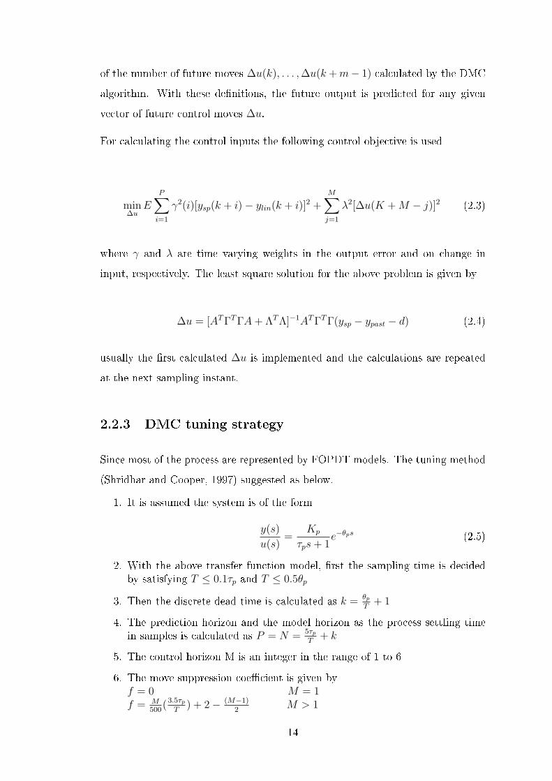
of the number of future moves ∆u(k), . . . ,∆u(k +m− 1) calculated by the DMC
algorithm. With these denitions, the future output is predicted for any given
vector of future control moves ∆u.
For calculating the control inputs the following control objective is used
min∆u
EP∑i=1
γ2(i)[ysp(k + i)− ylin(k + i)]2 +M∑j=1
λ2[∆u(K +M − j)]2 (2.3)
where γ and λ are time varying weights in the output error and on change in
input, respectively. The least square solution for the above problem is given by
∆u = [ATΓTΓA+ ΛTΛ]−1ATΓTΓ(ysp − ypast − d) (2.4)
usually the rst calculated ∆u is implemented and the calculations are repeated
at the next sampling instant.
2.2.3 DMC tuning strategy
Since most of the process are represented by FOPDT models. The tuning method
(Shridhar and Cooper, 1997) suggested as below.
1. It is assumed the system is of the form
y(s)
u(s)=
Kp
τps+ 1e−θps (2.5)
2. With the above transfer function model, rst the sampling time is decidedby satisfying T ≤ 0.1τp and T ≤ 0.5θp
3. Then the discrete dead time is calculated as k = θpT+ 1
4. The prediction horizon and the model horizon as the process settling timein samples is calculated as P = N = 5τp
T+ k
5. The control horizon M is an integer in the range of 1 to 6
6. The move suppression coecient is given byf = 0 M = 1f = M
500(3.5τp
T) + 2− (M−1)
2M > 1
14

7. Implement DMC using the traditional step response matrix of the actualprocess and the following parameters computed in steps 1-5:
• sample time, T
• model horizon (process settling time in samples), N
• prediction horizon (optimization horizon), P
• control horizon (number of moves), M
• move suppression coecient, λ
Tuning of unconstrained SISO DMC is challenging because of the number of ad-
justable parameters that aect closed-loop performance. Practical limitations of-
ten restrict the availability of sample time, T, as a tuning parameter.
Nevertheless moving horizon principle is the widely used technique in real time
control.
2.2.4 Principle of moving horizon MPC
An excellent overview of the state of the art on moving horizon based MPC is
given by Garcia et al. (1989), Camacho and Bordons (2004) and Goodwin et al.
(2004). Model predictive control systems consists of an estimator and a regulator
as illustrated in Figure 2.2. The inputs to the MPC are the target values, r, for
the process outputs, z, and the measured process outputs, y. The output from
the MPC is the manipulated variables, u.
MPC
y
ur
x
Regulator
Estimator
Plant
Sensors,Lab analysis
Figure 2.2: Generic model predictive control system.
The principle of moving horizon is given in Figure 2.3. MPC is based on iterative,
nite horizon optimization of a plant model. At time t the current plant state is
15

sampled and a cost minimizing control strategy is computed via a numerical mini-
mization algorithm as given in Equation (2.6) for a relatively short time horizon in
the future which is called as control horizon Nr. Specically, an online calculation
is used to estimate the projected trajectory over period of prediction horizon Ne
and nd a cost-minimizing control strategy until the length of control horizon.
Only the rst step of the control strategy is implemented, then the plant state
is sampled again and the calculations are repeated starting from the now current
state, yielding a new control and new predicted state path. The prediction hori-
zon keeps shifting forward and for this reason this is called as receding or moving
horizon control.
Figure 2.3: Principle of Moving Horizon MPC.
Normally MPCs are equipped with constraints on the manipulated inputs and
outputs. Constraints can be of two types: Hard constraints and soft constraints.
Hard constraints represent absolute limitations imposed on the system. These
names illustrate that hard constraints are to be necessarily satised and cannot
be violated. Soft constraints only express a preference of some solutions that
can be violated and is normally penalized heavily once they are violated. The
optimization methods for solving predictive control algorithms are described in
Maciejowski (2002).
16
2.3 Review of MPC in industries
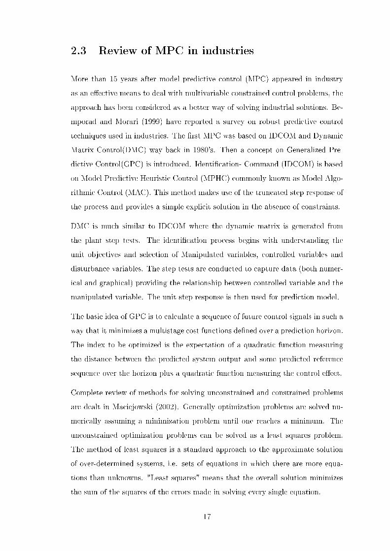
More than 15 years after model predictive control (MPC) appeared in industry
as an eective means to deal with multivariable constrained control problems, the
approach has been considered as a better way of solving industrial solutions. Be-
mporad and Morari (1999) have reported a survey on robust predictive control
techniques used in industries. The rst MPC was based on IDCOM and Dynamic
Matrix Control(DMC) way back in 1980's. Then a concept on Generalized Pre-
dictive Control(GPC) is introduced. Identication- Command (IDCOM) is based
on Model Predictive Heuristic Control (MPHC) commonly known as Model Algo-
rithmic Control (MAC). This method makes use of the truncated step response of
the process and provides a simple explicit solution in the absence of constraints.
DMC is much similar to IDCOM where the dynamic matrix is generated from
the plant step tests. The identication process begins with understanding the
unit objectives and selection of Manipulated variables, controlled variables and
disturbance variables. The step tests are conducted to capture data (both numer-
ical and graphical) providing the relationship between controlled variable and the
manipulated variable. The unit step response is then used for prediction model.
The basic idea of GPC is to calculate a sequence of future control signals in such a
way that it minimizes a multistage cost functions dened over a prediction horizon.
The index to be optimized is the expectation of a quadratic function measuring
the distance between the predicted system output and some predicted reference
sequence over the horizon plus a quadratic function measuring the control eect.
Complete review of methods for solving unconstrained and constrained problems
are dealt in Maciejowski (2002). Generally optimization problems are solved nu-
merically assuming a minimization problem until one reaches a minimum. The
unconstrained optimization problems can be solved as a least squares problem.
The method of least squares is a standard approach to the approximate solution
of over-determined systems, i.e. sets of equations in which there are more equa-
tions than unknowns. "Least squares" means that the overall solution minimizes
the sum of the squares of the errors made in solving every single equation.
17

The big problem with considering minima is that normally there may be many
local minima and the algorithm may stuck in one of the local minimum, unaware
of where the global minimum lies. Hence most of the optimization problems are
solved as convex problem. A convex optimization problem is one in which because
of convexity of the objective function, there is only one minimum or connected to
a set of equally good minima. Thus by solving convex problems global minimum
is always guaranteed.
Good general books and literatures on optimization are available. Fletcher (1987)
and Gill et al. (1981) have provided relevant material on optimization algorithms
especially for LP and QP methods. A whole book on using convex optimization
for control design is given in Boyd and Baratt (1991), however this book only talks
about solutions for convex optimization problems but does not deal with predictive
control. Convex problems are generally solved using quadratic program(QP). The
quadratic program is of the form
minθ
1
2θTΦθ + ϕT θ (2.6a)
s.t. Ωθ ≤ ω (2.6b)
Here the Φ is Hessian and normally θ is referred as error between the actual and
predicted value. If there are no constraints this is clearly convex if Hessian of the
objective function has to be positive semi-denite. Since the constraints are linear
inequalities, the objective function is a convex quadratic function.
A Linear Program (LP) is the special case of QP where the Hessian Φ = 0 in
Equation (2.6), so that the objective function is linear rather than quadratic. It
is also convex when Ω and ϕ are such that a minimum exists. In this case the
minimum always occurs at a vertex (or possibly an edge). Thus the constrained
objective function can be expressed as a convex object with at surface. This is
also known as simplex method. There are large number of standard algorithms
available for solving LP, one of the methods is simplex method.
Morari and Lee (1999) have investigated the evolution of controllers in the in-
dustries with PIDs being the most commonly used as it is well proven and then
18

the unconstrained control problems. When these controllers unable to handle the
complete industrial requirements, knowledge based controls and DMCs are used.
But the DMC formulation is completely deterministic and did not include any
explicit disturbance model. Then GPC is intended to oer a new adaptive control
alternative. But such controllers are not much suitable for multi-variable con-
strained systems which are more common in industries. Thus the work reviews
use of constrained MPCs based on linear MPCs used in industrial applications.
Real time applications of constrained MPC become feasible once the formulations
are solved either by LP or QP resulting in much faster controller response. In
order to improve the stability of such constrained systems works on 'contraction
constraints' are suggested.
Miller et al. (2000) have presented a case study on control of nonlinear systems
subject to constraints. A detailed approach on implementing Lyapunov functions
based control applications on nonlinear systems and the applications with labo-
ratory experiments are dened. The eectiveness of the resulting actions are also
demonstrated.
Brosilow and Joseph (2002) have proposed economic objectives of using con-
strained MPC in the industrial applications. In many of the applications it is
proposed that when the number of manipulated variables are more when com-
pared with the control variables it is desirable from the economic point of view to
have setpoints to the manipulated variables itself. Then a real time optimizer is
used to compute the economic target values for both the output and input vari-
ables, by including a cost term for inputs in the objective function. But this may
cause a steady state error in the system. To avoid such a situation it is proposed
to use multi loop control which provides a extra degree of freedom for moving the
inputs. In this chapter, in order to analyze the performance of conventional MPC
and soft MPC,each of the plant model parameters (gain, time delay, time constant
and zero) considered are varied one by one and the controllers are simulated with
the perturbed model.
The closed-loop performance of nominal linear model predictive control can be
quite poor when the models are uncertain. Consequently, some years after com-
19

missioning, many high-level control systems are turned o due to bad closed-loop
performance. This is often due to changes in the plant dynamics caused by wear
and tear combined with lack of the necessary human resources at the plant to re-
tune and maintain the MPC. Model predictive controllers with robust performance
against model plant mismatch is therefore crucial in long-term maintenance and
success of MPC system. Using soft output constraints in a novel way, the poor
performance of predictive control in the case of plant-model mismatch can be
improved signicantly.
A survey of reviews on model predictive controllers available in the industries is
given in Table 2.1
20

21
Table 2.1 Review of Model Predictive Controllers in Industries
S.No Author Problem Comments
1 Bemporad and Morari
(1999)
Reported survey of robust predictive control techniques in industries. Advantages and disadvantages of difference controllers(DMC, IDCOM, GPC) discussed
Complete review of different MPCs available in industries are discussed.
2 Morari and Lee (1999)
Reviews use of constrained MPCs based on linear MPCs used in industrial applications. Difference between unconstrained MPC and constrained MPC provided. Contraction constraints to improve stability.
Become feasible only if solved through LP or QP.
3. Miller et al., (2000)
Study of non linear systems subject to constraints. Detailed approach on Lyapunov functions implemented on non-linear systems. Laboratory experiments conducted to study the effectiveness in the control.
Complexity in calculation makes it least preferred in industrial applications.

2.3.1 Review on Tuning of MPC
Garriga and Soroush (2010) have provided a review of tuning guidelines for model
predictive control from theoretical and practical perspectives. A detailed review of
available methods to tune on DMC, GPC and state space representations and other
formulations such as MPL-MPC. General steps involved in tuning for increasing
the controller performances are discussed. Based on the formulation of control law
the tuning parameters have been discussed. O-line tuning methods are suggested
in which each parameters are individually tuned as given below.
• prediction horizon,
• control horizon,
• model horizon
• Weights on Outputs
• Weights on Rate of Change of Inputs
• Weights on the Magnitude of the Inputs
• Reference Trajectory Parameters
• Constraint Parameters
• Covariance Matrix and Kalman Filter Gain
Also review on auto tuning methods have been provided. The advantage of us-
ing an auto tuning is that the control engineer is not required to have a great
amount of system knowledge to initialize the tuning procedure. Also tuning pa-
rameters are update along with the optimization algorithm and thus they are set
to optimal values. Advances in covariance least- squares technology are expected
to make Kalman ltering much more accessible by automatically identifying the
main tuning parameters.
The challenges in process control and choosing an appropriate control strategy
for the respective applications have been discussed by Rhinehart et al. (2011).
This work is an editorial based on a presentation "Advanced classical or Model
predictive control?". Some of the important factors that attribute diculty in
industrial control like constraints, individuality of process, sensors, cause and eect
22

relations, initial capital const are discussed in detail. Also economic benets of
each controllers and usage of dierent applications like PID, PFC, ADRC, GMC
or PMBC for each processes depending on the operating conditions are provided.
The rst step involved in tuning is to develop an accurate process model. In all the
MPC frameworks development of perfect model will make the tuning procedure
much easier as it can be straight forward. If the controller performance is poor
then it must be considered the model is poor until proven otherwise.
2.3.2 MPC with Hard constraints
One of the advantages of using MPC over other controllers is it allows operation
closer to constraints compared with conventional controls, which leads to more
protable operation. Often these constraints are associated with direct costs, fre-
quently energy costs. For instance, in a manufacturing unit the power consumption
must be kept as minimum as possible with same level of production, this is a con-
straint on manufacturing process. Constraints can be present in both input as well
as output. Most commonly the input constraints on the control signals, that is
to the process or manipulated variables and rate constraints are hard constraints.
This may be because of various reasons like saturation, physical limitations etc.,
These constraints can never be violated.
For example in Equation (2.6), the inequality constraints
"Ωθ ≤ ω"
is called hard constraints as the condition needs to be strictly satised when cal-
culating the optimization solution. The best example of hard constraints in real
time is the high and low limit of the manipulated variables which cannot be varied
beyond the limits because of the physical restrictions like vibrations etc.,
Clarke (1988) has proposed a generalized model predictive controller with hard
input constraints. The controller is based on the minimization of long-range cost
function. The model used for controller is CARIMA model. The closed loop
performance of the controller is investigated using simulation.
23

Iino et al. (1993) have proposed a new method by modifying the Generalized
predictive control. Firstly, a Kalman lter based predictor is introduced in order to
improve the robustness of the predictor against noises. Secondly, a time-dependent
weighting factor is introduced into the MPC's quadratic type cost function, in
order to improve the transient response characteristics. Thirdly, a parameter
tuning method is proposed that adjusts the weighting factors in the cost function
considering robust stability of the control system. Finally, the proposed MPC
method with and without constraint conditions that are the upper/lower limits
and rate limits for both manipulation variables and process control variables, is
formulated. The controller is tested in an ethylene plant's dynamic simulator. The
models are obtained by simple step tests in the plant. ARMA types of models are
used for prediction.
A design method of LQ optimal control law is considered for constrained continuous-
time systems by Kojima and Morari (2004). Here the control laws are obtained
based on quadratic programming. The control law converges to exact solutions
by introducing singular value decomposition for nite-time horizon linear systems.
By employing the control problem to a double integrator with constraints it is clar-
ied that the receding horizon control is equivalent to that of the state feedback
control where the gain is calculated by a piecewise ane state functions.
Guzman et al. (2009) have provided a solution for output tracking problem for
uncertain systems subject to input saturation. In order to tackle constraints and
modeling errors an external supervisory control method is proposed. Thus a cas-
cade loop with any type of inner control and a GPC for outer loop is considered.
A robust constrained Linear Matrix Inequality (LMI) based approach is developed
as a solution to control such systems. The existing control loop is rst converted
into state space representation and LMI is used to provide state space feed back
for the inner loop controller. The controller is then tested in an integrator plant
with delay with a inner loop PI controller. The inner control loop is studied with
PI controller in the presence of uncertainties and it is found that stability prob-
lems occur. Then the controller is included with the GPC for controlling the inner
loop considering input saturation and it is found that the performance results also
24

ensuring constrained robust stability.
A survey of some of the reported work on the model predictive controllers with
hard constraints relevant to the present work is given in Table 2.2
25
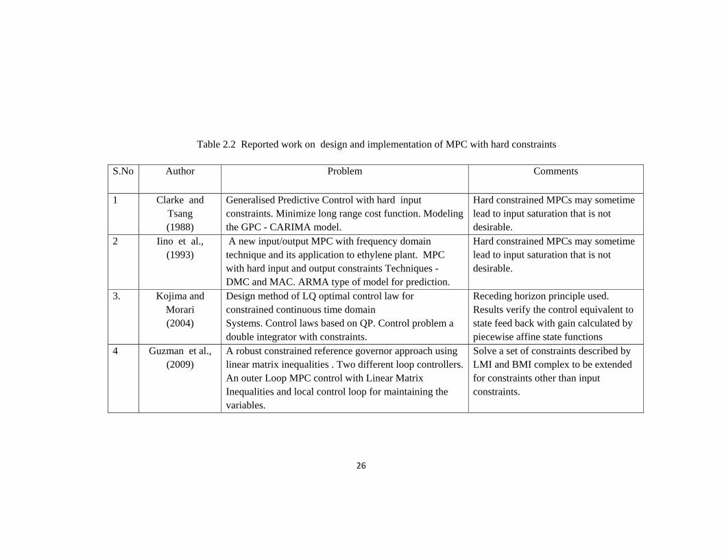
26
Table 2.2 Reported work on design and implementation of MPC with hard constraints
S.No Author Problem Comments
1 Clarke and Tsang (1988)
Generalised Predictive Control with hard input constraints. Minimize long range cost function. Modeling the GPC - CARIMA model.
Hard constrained MPCs may sometime lead to input saturation that is not desirable.
2 Iino et al., (1993)
A new input/output MPC with frequency domain technique and its application to ethylene plant. MPC with hard input and output constraints Techniques - DMC and MAC. ARMA type of model for prediction.
Hard constrained MPCs may sometime lead to input saturation that is not desirable.
3. Kojima and Morari (2004)
Design method of LQ optimal control law for constrained continuous time domain Systems. Control laws based on QP. Control problem a double integrator with constraints.
Receding horizon principle used. Results verify the control equivalent to state feed back with gain calculated by piecewise affine state functions
4 Guzman et al., (2009)
A robust constrained reference governor approach using linear matrix inequalities . Two different loop controllers. An outer Loop MPC control with Linear Matrix Inequalities and local control loop for maintaining the variables.
Solve a set of constraints described by LMI and BMI complex to be extended for constraints other than input constraints.

2.3.3 Soft Constrained MPC
In many of the constraint control problems the controller solutions become infea-
sible because of the hard constraint violation problems which may be result of
various factors in real time. State and output constraints may lead to infeasibility
of the optimization problem. For example, an output disturbance may push the
output out the feasible region such that no feasible input trajectory is able to
bring in back in the constraint region. In that case the hard output constraints
can no longer be maintained. The soft constrained MPC explained above mostly
take care of the eects due to the disturbances of the system.
One systematic strategy for dealing with infeasibility is to soften the constraints.
That is, rather than regard the constraints as hard boundaries which can never
be crossed, to allow them to be crossed occasionally but only if necessary. Usually
input constraints are hard constraints and there is no way in which they can
be softened, like actuator limits. Maciejowski (2002) has provided a detailed
explanation of how to use soft constraints in the optimization problem. A possible
way to proceed is to discard the output constraints that cause the infeasibility.
A more subtle way that tries to bring the output back in the feasible region is the
use of a slack variable ϵ.
The slack variable is introduced to relax the constraints that cause the infeasib-
lity according to the normal hard constraint formulation Ax.b + ϵ. Additionally,
a term ϵTQ3ϵ is added to the cost function where Q3 > 0 is some positive def-
inite weighting matrix. The slack variables are treated as free variables and are
optimized such that on the one hand the infeasible constraints are relaxed and
on the other hand the constraint violation is minimized. The optimization prob-
lem remains a quadratic programming problem because the new variables ϵ are
introduced quadratically in the cost function and linearly in the constraints.
Scokaert and Rawlings (1999) have proposed a state based soft constraint approach
for handling the infeasibility with respect to conventional predictive control ap-
proach. Two types of solutions are provided for such systems, a minimal time ap-
proach and a soft constraint approach. It is illustrated by using a non- minimum
27

phase system that state constraints will be included when the solution becomes
infeasible. In the rst approach the control algorithm identies the smaller time
in which the state constraint can be satised and in the second method a soft
constraint approach where the controller penalizes for state constraints violation.
The closed loop and open loop responses of both the approaches are investigated.
It is found that in both the cases the controller performance are close to Pareto
optimal. Also soft-constraint MPC formulations are nominally exponentially sta-
bilizing and asymptotically stabilizing under decaying perturbations. The main
drawback of such controllers are they require larger QP solutions resulting in
slower response which may not be feasible in real time.
Kerrigan and Maciejowski (2000) have proposed a MPC method, in which the
hard constrained MPC is converted into soft constrained by introducing a slack
variable on the states. A slack variable is included in the objective function with
moving horizon principle when the controller solutions become infeasible during
the hard constraint approach. The MPC problem is treated as a multi-parametric
quadratic program (mp-QP) and exact penalty functions are introduced in order to
nd a condition on the lower bound for the violation weight. By introducing slack
variables the non-smooth, exact penalty function can be converted into a smooth,
soft-constrained QP problem. It is shown from examples that if the constraint
violation weight that is used in the soft-constrained cost function is larger than
the maximum norm, the solution is guaranteed to be equal to the hard-constrained
solution for all feasible conditions that were considered.
Bemporad et al. (2002) have proposed a feedback control law to minimize a
quadratic performance criterion. Here the control law is piecewise linear and
continuous for both the nite horizon problem with model predictive control and
innite time measure for constrained linear regulation. A LQ regulator algorithm
is developed with hard constraints. But in order to avoid feasibility problem out-
put constraints are softened /relaxed. The stability of the controller is analyzed
and found satisfactory as MPC. One advantage of such technique is that it can
be implemented without any online computations, but cannot be applied for large
scale applications.
28

Another method on range control explained by Roubal and Havlena (2005) and
Havlena and Lu (2005) provide a soft limit band for the output where the controller
does not react for change in output within the region. The basic idea of range
control approach is to replace the set point of controlled variable Y by a set range
which is dened by the sequence of low and high limits yL and yH as given in Figure
2.4. Then the optimality criterion can be expressed as a quadratic programming
Figure 2.4: Penalty function and modied penalty function of Range control, yL =−1 yH = 1 .
problem as given by Equation 2.7.
minθ
1
2∥yk − Suk − wk∥2Qy
+ ∥∆u∥2Qu(2.7a)
s.t. yL ≤ wk ≤ yH (2.7b)
Thus the controller acts only when the controlled variables are beyond the range
of constraints. In order to avoid steady state oset because of no action within
the band the controller is solved by least squares solution whenever the controlled
variables are within the band. The controller is implemented in distributed pa-
rameters system which is described by a linear two-dimensional (dependent on
two spatial directions) parabolic partial dierential equation.This partial dieren-
tial equation is transformed to the discrete state space description using the nite
dierence approximation. A model with a large dimension is obtained and has to
be reduced for an advanced control design. The balanced truncation method is
used for the model dimension reduction. The challenges faced when using range
29

control methods are discussed and such methods always leave oset like a normal
dead band controller. So a modied penalty function is included. Most of the soft
constraints are for state constraints where the internal state of the system gets
disturbed because of the various disturbances A detailed study on the real time
implementation of the control method in industries is made.
A survey of important work on the model predictive controllers with soft con-
straints is given in Table 2.3
30

31
Table 2.3 Reported work on design of soft constraint based Model Predictive Controllers
S.No Author Problem Comments
1 Scokaert and Rawlings
(1999)
State soft constraint based MPC. For achieving feasibility two approaches are provided.
1. Minimal time approach 2. Soft constraints approach.
A minimal time approach and soft-constraints approach are provided. A penalty term for compensating the violations.
Only if the model of the system reflects the state perfectly. Require larger QP solutions resulting in slower response which may not be feasible in real time.
2 Kerrigan and Maciejowski
(2000)
Soft constraints based on the range of penalty function. Behaves as soft constrained MPC and hard constrained MPC on constrained violations. MPC to discrete-time LTI state space model, soft constraint as slack variable
QP dependent on both current state, previous control input and reference trajectory. This may not be feasible all solutions.
3 Bemporad, Morari et al.,
(2002)
A LQ regulator algorithm with hard constraints. To avoid feasibility problem hard output constraints are softened or relaxed. A piecewise linear solution is provided for the linear QP. The feasibility of the control mainly depends on initial state.
Cannot replace the large scale MPC as it cannot handle all the situations satisfactorily.

32
Table 2.3 (contd.. )
4 Roubal and Havlena (2005)
The control objective include simple range control objective along with other hard constraints. The controlled variable setpoint replaced by sequence of low and high limits.
A dead band controller based on QP. Can leave offset as there is no action for outputs within the band
5 Havlena and Lu
(2005)
Range control for disturbance adsorption problem. A penalty function for the outputs within a specified range. Implemented in distributed parameter system described by two dimensional parabolic partial differential equation.
Power and chemical/ refining industries need such integration for providing long term production and energy efficiencies.

2.3.4 Robust Model Predictive controllers
A controller is said to be robust which are designed for a particular set of param-
eters if it would also work well with dierent sets of parameters. Thus a robust
controller is one which can handle systems with uncertainties or disturbances ef-
fectively. Robust methods aim to achieve robust performance and/or stability in
the presence of bounded modeling errors.
Warren and Marlin (2004) have proposed controller solves a second-order cone
program (SOCP) at each execution in order to determine the set of control moves
that will optimize the expected performance of the closed-loop system while main-
taining the uncertain process outputs and inputs within their allowable bounds.
The proposed formulation uses a probabilistic, closed-loop description of system
uncertainty that is calculated o-line. On-line, the MPC requires the solution of
a convex second-order cone program that can be eciently solved with existing
interior-point algorithms. The controller discussed avoids this limiting assumption
while maintaining robust output constraint handling. The process is assumed
to be linear time-invariant (LTI) within the prediction horizon. The controller
deals with plant-model uncertainty by replacing deterministic constraints. Here a
method for eectively handling probabilistic input constraints is proposed. Also
the system uncertainty is split into several uncertainty regions. The uncertainty
associated with each region is smaller than the total system uncertainty, allowing
each subset to approach the input constraint more quickly. This reduces the "
back-o" caused by the probabilistic input constraints. Case studies illustrate the
improved dynamic performance of the multi-region method. The experimental
results are veried using a 1st order, isothermal CSTR along with modeling error.
From experimental methods it is proven that the robust controller can handle
uncertainties quite eectively.
Kassmann et al. (2000) have presented a new formulation of the steady-state tar-
get calculation that explicitly accounts for model uncertainty. When model uncer-
tainty is incorporated, the linear program associated with the steady-state target
calculation can be recast as a second order cone program. Also the advantages
33

of primal-dual interior-point methods in the resulting structure is discussed. The
mathematical parameterizations of possible plants is known as the uncertainty
description. It can take many dierent forms and can be given parametrically or
statistically. A heavy oil fractionator with 2 × 2 model is taken for simulation
comparison. The closed loop comparison is made between nominal LP and robust
LP. This SOCP can greatly improve control by rigorously accounting for modeling
uncertainty. The resulting SOCP structure can be exploited to develop ecient
numerical solutions based on primal-dual interior-point methods.
A survey of some of the important work on robust model predictive controllers
available for handling uncertainties is given in Table 2.4
34

35
Table 2.4 Reported work on Robust MPC based on Second Order Cone Programming Technique
S.No Author Problem Comments
1 Warren and Marlin
(2004)
SOCP based MPC for handling uncertainty has been proposed. Deals with probabilistic output constraints solved in offline. SOCP solved using efficient interior-point algorithms. A 1st order , isothermal CSTR considered along with modeling error. Case studies illustrate the improved dynamic performance of the multi-region method
A robust MPC using SOCP implemented by simulation and need to be modified to match the industrial approach.
2 Kassmann and
Badgwell (2004)
The MPC algorithm is steady-state target for accounting model uncertainty using SOCP calculation followed by dynamic optimization. A heavy oil fractionator with 2 x 2 model taken for simulation comparison.
SOCP can greatly improve control by rigorously accounting for modeling uncertainty.
2.4 Ball Mill Control
Researchers have been working in optimizing the ball mill grinding process along
with the separation process. Various studies have been done for analyzing the
dynamics of the ball milling circuit. The electrical energy consumed in the cement
production is approximately 90 kWh/tonne. 30% of the electrical energy is used for
raw material crushing and grinding while around 40% of this energy is consumed
for grinding clinker to cement powder as given by Fujimoto (1993); Jankovic et al.
(2004). Global cement production use approximately 2% of the worlds primary
energy consumption and 5% of the total industrial energy consumption as reviewed
by Concil (1995) and Austin et al. (1984). Also ball mill is one of the dicult
Rajamani and Herbst (1991a) have proposed feedback and optimal control meth-
ods for optimizing ball mill grinding circuits. Here the ball mill considered was an
semi-autogenous mill which is a wet method of grinding compared to normal dry
grinding circuits. Rajamani and Herbst (1991b); Herbst et al. (1992) have devel-
oped dynamic and simplied models of the cement mill circuit. Based on these
modeling, two PI controllers were tuned and an optimal control was designed. The
model was developed by introducing step changes in the real time system. The pa-
rameters considered are online particle size distribution with respect to fresh feed
rate and sump level. First a feedback control based on maximization principle is
designed for increasing the feed rate and an optimal control based on minimizing
the integral square error was developed. Both the controllers were tested rst in
simulator and then in real plant. From the real time results it was shown that the
settling time of optimal controller was around 6 min when compared with feed
back controller (26 min). Also the Feed back control exhibited oscillations with
an ISE value of particle size is 16.6 whereas optimal control had an ISE value of
8.5 which is almost half that of the Feed back control.
Van Breusegem et al. (1994) and Van Breusegem et al. (1996a) have proposed a
model based algorithm for the regulation of cement mill circuit. The controller
was based on Linear Quadratic algorithm. Here a black-box model was developed
based on the experimental data collected from the simulation. The dynamic model
36

in the form of four rst order dierential equations were converted into state space
to be used in LQ control. Integral actions were added for making the control oset
free. A dynamic simulator was developed based on the models and the controller
performance was compared with PI controller and from the results it was shown
that the standard deviation of quality had been reduced and also the variation in
tailings were also less.
Boulvin et al. (2003) have developed a grey box model with algebraic and par-
tial dierential equation with unknown parameters for cement grinding process .
Through experimental data the unknown parameters were estimated and a dy-
namic simulator was developed to analyze the control and process behavior in real
time operation. Two controllers PI and LQ control developed by Van Breusegem
et al. (1994) were compared with the simulated model. Then a cascaded control
for regulating mill ow rate and simple PI control for neness control was ap-
plied. Incase of online measurement of recirculation ow a Feed forward controller
was proposed. Here the feed-forward provide best results in terms of mill ow
regulation. But since the diculty in online measurement cascade control was
considered as best solution.
Ramasamy et al. (2005) have developed input/output models through step re-
sponse tests in simulator. Multi loop PI was designed and decoupled to account
for interaction between the control loops. The de-tuning factor was based on IAE
of output variables. The model predictive control from MATLAB was compared
with PI and from the results it was shown that the MPC achieves better decou-
pling. Then constraints were included in the model using MATLAB toolbox. From
the results it was conrmed that the constrained MPC provides sluggish operation
than unconstrained but it provides a much better decoupling. Also the MPC was
compared with decoupled PI controllers and the results showed that PI controller
results in more oscillations and longer settling time.
Conventionally, the grinding circuits are controlled by multi-loop PID controllers,
but these controllers generally have drawbacks, such as input/output pairing prob-
lems and hard tuning work. Chen et al. (2009) have provided an adaptive DMC for
handling ball mill grinding circuit with multiple model developed based on three
37

dierent SOPDT transfer function models. The 3 × 3 MIMO transfer function
system was developed using step response test. A simple DMC objective function
was considered and the models were switched depending on the input variation
ranges. The performance of DMC compared with PI and it was found that the
quality variations were reduced by 3%
Chen et al. (2008) have developed constrained DMC for controlling ball mill pro-
cess. The real time implementation of 3× 3 MIMO transfer function model based
on step response tests. In addition to normal DMC objective function, hard con-
straints on manipulated variable, rate of change of manipulated variable and con-
trolled variable were included. The prediction horizon was selected as P = 20
and control Horizon as M = 5. From the results it was shown that the online
measurement of quality is improved from 88% to 95%.
Martin and McGarel (2001) have proposed Nonlinear MPC for controlling the real
time cement mill circuit. Here the NMPC process gains were calculated based on
model from neural networks. Data from plant was obtained to train the neural
network model and this provide non-linear process gain for NMPC. Also maxi-
mum and minimum gains were also calculated. Hard constraints on manipulated
variable and rate of change in manipulated variables were also included. From the
results it was reported with such type of control the product quality consistency
was close to 95%.
A summary of reported work on Survey on model predictive controllers available
for control of ball mill circuits is given in Table 2.5
38

39
Table 2.5 Reported work on Model Predictive Controllers for ball milling processes
S.No Author Problem Comments
1 Rajamani and Herbst (1991a)
Feedback and optimal control methods for optimizing ball mill grinding circuits.Semi-autogenous mill considered for control. Models developed by Rajamani and Herbst (1991a) used. Optimal control based on minimization of ISE tested with Feedback control based on maximization principle.
Optimal control perform better than Feedback control. Constraints not considered in the controllers.
2 Van Breusegem et al. (1994) and Van Breusegem
et al. (1996a)
Model based algorithm for the regulation of cement mill circuit. Controller based on LQ algorithm. Black-box model based on simulation data reduced to first order differential equations.
Controller compared with PI control and standard deviation in quality is reduced.
3
Boulvin et al. (2003)
Agrey box model with algebraic and partial differential equation with unknown parameters for cement grinding process. Unknown parameters estimated through simulation data. PI and LQ controllers compared with simulated model.
feed-forward provide best results in terms of mill flow regulation. Diffculty in online measurement, so cascade control considered as best solution.

40
Table 2.5 (contd.. )
4
Ramasamy et al.
(2005)
Developed input/output models through step response tests in simulator. Multi loop PI designed and decoupled. MPC compared with PI controller in MATLAB toolbox .
Constrained MPC sluggish in operation but provides much better decoupling. PI controller results in more oscillations.
5
Chen et al. (2009)
An adaptive DMC for handling ball mill grinding circuit with multiple model developed based on three different SOPDT transfer function models. This avoid input/output pairing problem.
Unconstrained DMC is better than PI control but cannot be used interms of constraints and uncertainties.
6. Chen et al. (2008)
Constrained DMC for controlling ball mill process. real time implementation of 3×3 MIMO transfer function model. Hard constraints on MVs, rate of change in MVs and CVs along with objective function
Results compared with unconstrained DMC and found to increase the standard deviation in quality variations. Can be implemented only with online measurement of quality.
7. Martin and McGarel (2001)
Nonlinear MPC for controlling the real time cement mill circuit. NMPC process gains calculated based on model from neural networks. Data from plant obtained to train the neural network model and this provide non-linear process gain for NMPC. . Hard constraints on MVs, rate of change in MVs included.
Quality consistency improved with such controllers. But difficult to be used in real time because of computational complexity and modeling

2.4.1 Cement Mill modeling
The main problem with such control techniques are that the controller performance
degrades with plant-model mismatch. Researches have been working in the area
of modeling to improve the performance of such controls.
The closed loop ball mill-classier grinding circuit has been described by lumped
model (Benzer et al., 2001). Here the lumped model specically includes the mill
load (amount of material inside the mill) as a state variable. Another way of
modeling the cement milling circuit is based on the input/output characteristics
of the milling process which can be considered as a black-box model as presented
by Lepore et al. (2002, 2003, 2004, 2007a,b) in their various works.
Discrete-element model techniques have been developed by Cleary (2006), Powell
and McBride (2006) and Jayasundara et al. (2008) which can be used to provide
information on the radial dynamics of the materials and also the axial distribution
of the dierent particle sizes within the discharging ball mill. This facilitates the
clear understanding on the estimation of power draw and of liner wear inside the
ball mill.
Neural network is one of the methodology used for determining the black-box
model, the cement mill modeling based on neural networks has been developed by
Martin and McGarel (2001) and Topalov and Kaynak (2004). The main advan-
tage of using black-box model is the occurrence of non-linear behavior with the
input/output parameters considered for modeling. The non-linear behavior can be
made just complex enough for the description of the main process dynamics while
remaining tractable for control design as given by Huusom et al. (2005), Efe and
Kaynak (2002) and Grognard et al. (2001). But these models are quite dicult
to be implemented in the real time systems, because of the complexity in design
and diculty to be coupled with control algorithm. Thus it is required to reduce
the models to lower order to be used in control applications which will result in
loss of important dynamics in the system.
41
2.5 Fuzzy Logic Controller in Cement Industries
In general, the most widely used technique in cement industries for optimization
is based on Fuzzy Logic. The control rules of the fuzzy controller are obtained
from the knowledge of the operators. These types of controllers are used in cement
plant widely because they do not require mathematical/ empirical model of the
plant and can be easily congured even for non-linear systems.
ZimmerMann (1996) has given an overview of current applications of Fuzzy control
to real world problems. A brief discussion of Fuzzy control systems for rotary
cement kiln has been provided. The main problem in mathematical modeling
control strategy is that the relationships between input and output variables are
complex, nonlinear. The control variables chosen are exhaust gas temperature,
burning zone temperature, oxygen percentage and liter weight. The manipulated
variables are coal feed rate, kiln fuel and induced draught fan speed. The aim
of the kiln control is to automate the routine control strategy of an experienced
operator. After discussions with operators, 75 operating conditions as fuzzy are
dened as drastically low, low, slightly low, ok, slightly high, high and drastically
high. Fuzzy rules are written to change the drive load, fan speed and fuel for
maintaining the above control variables.
Cao et al. (2008) have proposed a high precision sampling fuzzy logic controller
with self-optimizing to the cement ball mill circuit. This controller, based on fuzzy
control strategy, improves the control precision by a fuzzy interpolation algorithm.
The fuzzy logic controller and the self optimizing algorithm along with sampling
and interpolation algorithm are implemented in a MATLAB simulator with a
second order plus dead-time model which demonstrates the ball mill circuit. Fuzzy
rules are altered to make the control parameter reach steady state without steady
state error. In addition, the high precision sampling fuzzy logic controller has been
put into practice in the clinker cement production workshop of a cement mill. The
rules are altered as per real time and it is found that the power consumption is
decreased and the particle size distribution becomes standard.
Wardana (2004) has proposed a Fuzzy-PID controller for maintaining the under
42

grate pressure by varying the grate speed. Here the classic representation of
Mamdani logic operations are applied, a 7×7 rule of fuzzy algorithm and centre of
area for defuzzication are implemented. The performance of the FLC is compared
with conventional PID controller. It has been found that the standard deviation
of under grate pressure has been reduced from 50 mmH2O to 5 mmH2O and also
the temperature of clinker output is reduce from around 150oC to around 90oC.
Lin and Chin (1996) have proposed an application of fuzzy logic inference tech-
nique on a cement grinding roller control. The control of cement grinding roller is
that the oil-pressure is commanded to follow a desired setting pressure. A neural
network scheme is applied to identify the system model for establishing the sim-
ulation program for evaluating the derived control algorithm and the fuzzy rules
are proposed to infer the desired setting pressure to replace the original PI-like
method. The controller is applied in real time cement plant and it is found that the
stability of operation has been improved signicantly with the proposed control
technique.
The Fuzzy Logic Controller used for comparing the performance of soft MPC is
a commercial package available in FLSmidth's Process EXpert system(Automation
(2008)). It has been widely used in industries for controlling various cement plant
applications over the years. The controller is already available in the cement plant
and has been used directly for comparing the soft MPC.
From the above literatures it can be viewed that the control strategies used for
cement mill circuit are based on the models obtained from the plant and there is
no detailed study on plant-model parameter mismatch. Normally, cement circuits
are characterized by large uncertainties because of input material variations and
mechanical wear and tear over the period of time. Also the controllers consider
only online measurements and infer the quality parameters for control, which is
quite uncommon in real plant. This will aect the success of such controllers in real
time.The work on robust MPCs provided in the literatures have not been tried in
controlling real time cement mill circuit. Thus there is a need for design of robust
MPC and develop MPC based on soft constraints to address the uncertainties
present in the cement mill.
43

CHAPTER 3
An evaluation of existing MPC tools
In this chapter, the eect of uncertainties on an unconstrained Dynamic ma-
trix Controller similar to the one proposed by Cutler and Ramakar (1980) is
investigated. Prasath and Jorgensen (2008) have proposed a predictive con-
troller based on FIR models with 'ℓ2' regression norm, including the regulariza-
tion weights (R and S)(denoted as regularized l2 nite impulse response (FIR)
predictive controller) along with input and input-rate constraints. Feedback from
estimator is based on a simple constant output disturbance lter. Prasath and
Jørgensen (2009) have proposed a moving horizon constrained regularized ℓ2 es-
timator (MHE) based on nite impulse response models (FIR). The performance
of the controller with both the simple estimator and Moving horizon estimator
in the face of plant-model mismatch is simulated using a SOPDT with a zero
transfer function model. Then the work by GuruPrasath and Jorgensen (2009)
on the controller equipped with soft output constraints that are used to have ro-
bustness against model plant mismatch is investigated. The simulations can be
used to benchmark ℓ2 MPC against FIR based robust MPC as well as to estimate
the maximum performance improvements by robust MPC. The bench mark study
includes
• The performance of the controllers in the presence of uncertainties in thesystem and the disturbances in the system
• Handling the infeasibility involved in solving the constraint problem.
3.1 Introduction
Dynamic Matrix Control (DMC) was the rst Model Predictive Control (MPC)
algorithm introduced in early 1980s. Nowadays, DMC is available in almost all
44

commercial industrial distributed control systems and process simulation software
packages.
DMC based on step response coecients for blast furnace has been dealt by Cutler
and Ramakar (1980). The DMC is represented with a set of numerical co-ecients
based on step test. The technique is conjunction with minimizing the integral
of error/time curve. The controller developed is compared with existing PID
controller in the plant for handling dead time. Future moves on actuator and
the corresponding future measurements are predicted using a method similar to
moving horizon principle. Here the step response co-ecients are used to update
the dynamic matrix and the feed back is taken from real data, but not based on
estimation.
In Prasath and Jorgensen (2008), FIR based MPC is developed for industrial
control purpose (especially with cement plant application) where the system in-
cludes both process and measurement noise, the analysis on performance of the
controllers in a stochastic system is made. Maraoti et al. (2010) have proposed
a recursive least squares based persistently exciting MPC by referring this work
on FIR based MPC.
The eect of uncertain models on the performance of a regularized ℓ2 model pre-
dictive controller with input constraints, input-rate constraints and soft output
constraints have been investigated by Maciejowski (2002), Goodwin et al. (2005)
and Qin and Badgwell (2003).
In contrast to state space parameterizations, the FIR model is in a form that
can easily be applied in robust predictive control, i.e. predictive control based on
robust linear programming or second-order cone programming, the work on such
programming have been explained by Hansson (2000) and Vandenberghe et al.
(2002). The predictive control based on second-order cone programming have
been investigated by Ben-Tal and Nemirovski (2001) and Boyd and Vandenberghe
(2004).
The controller performance can be improved by using a FIR based moving hori-
zon estimator where the unmeasured disturbances are estimated based on the
45

measured outputs and fed back into the controller.
The advantage of FIR parametrization is that it is both linear in parameters (im-
pulse response coecients) and the decision variables. In the regulation problem,
decision variables are the manipulated variables, while the decision variables in
the estimation problem are the known process disturbances. In addition, the -
nite impulse response parametrization also yields a band structured Hessian in the
resulting quadratic program that can be used for its ecient solution.
Based on linear models Muske and Rawlings (1993b) have used a moving hori-
zon estimator and used input or output disturbances to have a steady state oset
free control. Robertson and Lee (1995) and Robertson et al. (1996) have pre-
sented moving horizon estimators for nonlinear systems and relate the optimization
based approach of moving horizon estimation to a probabilistic state estimation
approach. Rao et al. (2001) have proposed sucient conditions for the stability
of moving horizon state estimation with linear models subject to constraints on
the estimate. Rao and Rawlings (2002) have illustrated using a series of example
monitoring problems, the practical advantages of MHE by demonstrating how the
addition of constraints can improve and simplify the process monitoring problem.
All these methods cited above are based on state space approach. In Prasath
and Jørgensen (2009), a method based on convolution approach is adopted for
the estimation of unknown disturbances from the measurement outputs. The
estimator produces non-smooth disturbance estimates upon which the regulator
reacts and introduces real output variations by its manipulation of the process
inputs. The simulations are used to critically address the performance limitations
in case of measurement noise.
In most of the literatures reported,the soft constraints are included in the system
when the hard constrained optimization problem has no solution because of ei-
ther process conditions or disturbances in the system. The soft constraints are
introduced as a slack variable and they become active only if the original hard
constrained solution becomes infeasible. In GuruPrasath and Jorgensen (2009),
the slack variables on soft constraints are included in the regular objective func-
46

tion and the optimization is solved in real time. Here the slack variables are used
as dead band across the reference variable, which improves the robustness of the
controller by providing two dierent solutions one within the dead-band and the
other outside the band. This technique is similar to the technique that have been
proposed by Honeywell technologies in RMPC (Qin and Badgwell, 2003; Havlena
and Lu, 2005; Havlena and Findejs, 2005) where a funnel type objective func-
tion is solved. Compared to classical control, the use of soft constraints has some
similarities to PID control with dead zone as given by Shinskey (1988).
In this chapter, initially the performance of the controllers are simulated using a
generic SOPDT with zero transfer function model of the system for SISO case.
MIMO simulation system the model is obtained from the available cement mill
circuit simulation for which the details are given in later chapters.
3.2 Dynamic Matrix Control(DMC)
The major elements of DMC are (i) the model, (ii) estimation of the disturbance
and projection into the future and (iii) computation of control inputs. The model
used is a discrete truncated step response model. The basic formulation of DMC
has been given by Camacho and Bordons (1999). The DMC reported in section
2.2.2 is implemented on a FOPDT transfer function.
Based on the tuning methods suggested, the control parameters formulated for
the DMC are Sampling Time - 0.1, Prediction Horizon - 20, Moving Horizon
- 10, Simulation Length - 200, the smoothing factor is varied between 0.0 and
0.7 to smoothen the prediction values based on moving average and to analyze
the performance of the controller for dierent ranges of smoothing factors. The
smoothing factors are used to smoothen the prediction, based on the moving
average principle and two values of smoothing factor α = 0 and α = 0.7 are used
to provide variations in the prediction.
First the performance of the DMC is analyzed by tuning the control weights
λ = 0.1, 1, 10, 100, 1000 as given in Figure 3.2. This is done to nd the optimum
47

0 50 100 150 200−0.5
0
0.5
1
1.5Control Weight λ=0.1
α=0
α=0.7
Out
put
0 50 100 150 200−0.5
0
0.5
1
1.5
time, min
Inpu
t
0 50 100 150 200−0.5
0
0.5
1
1.5Control Weight λ=1
α=0
α=0.7
Out
put
0 50 100 150 200−0.5
0
0.5
1
1.5
time, min
Inpu
t
0 50 100 150 200−0.5
0
0.5
1
1.5Control Weight λ=10
α=0
α=0.7
Out
put
0 50 100 150 200−0.5
0
0.5
1
1.5
time, min
Inpu
t
0 50 100 150 200−0.5
0
0.5
1
1.5Control Weight λ=100
α=0
α=0.7
Out
put
0 50 100 150 200−0.5
0
0.5
1
1.5
time, min
Inpu
t
0 50 100 150 200−0.5
0
0.5
1
1.5Control Weight λ=1000
α=0
α=0.7
Out
put
0 50 100 150 200−0.5
0
0.5
1
1.5
time, min
Inpu
t
Figure 3.1: Performance of Dynamic Matrix controller for step responses with dif-ferent control weights λ = 0.1, 1, 10, 100, 1000.
48

0 50 100 150 200
0
1
2
MPC− Model with Nominal Delay
α=0
α=0.5
Out
put
0 50 100 150 200
0
1
2
time, sec
Inpu
t
0 50 100 150 200
0
1
2
MPC− Model with Uncertain Delay(τd = 3)
α=0
α=0.5
Out
put
0 50 100 150 200
0
1
2
time, sec
Inpu
t
0 50 100 150 200
0
1
2
MPC− Model with Uncertain Delay(τd = 9)
α=0
α=0.5
Out
put
0 50 100 150 200
0
1
2
time, sec
Inpu
t
Figure 3.2: Performance of the DMC with uncertainty in delay with control weightλ = 10.
weight for nominal model and the same weight is used for analysis of performance
of the controller during plant-model mismatch. Here the DMC is made online in
a closed loop based on the state space model obtained from the FOPDT transfer
function as in Equation 3.1.
G(s) =1
(5s+ 1)e−5s (3.1)
The step response coecients for the controller are also extracted from the same
transfer function (Equation 3.1).
From Figure 3.1, it can be observed that when the control weight is 0.1 the con-
troller is quite unstable as there is no restriction in input moves resulting in huge
variations in the output, and when the control weight is increased the input moves
of the controller are restricted and thus reduces the oscillations in the output. But
49
as the control weights are extremely high the control moves become sluggish and
the output never settles when the control weight is 1000. Thus from the Figure
3.1 it is clear that when the optimum control weight for smooth performance of
DMC with the FOPDT model is λ = 10.
The performance of the DMC is then studied for the system with model uncer-
tainty. As a case study, the DMC is tested with models with time delay uncer-
tainty. Figure 3.2 shows the performance of the controller when the time delay of
plant model is same as nominal model for optimum tuning conditions. When the
time delay of plant model is dierent from the controller model the behavior of
the MPC is seen in the Figure 3.2. For nominal model the settling time is around
60s. When the time delay of plant model is higher than the nominal model the
performance of controller completely deteriorates and the control actions become
oscillatory and the MPC becomes unstable when the plant delay becomes almost
double the time delay in nominal model. Although DMCs are quite simpler in
approach and less complex, since the extension of DMC cannot be used for robust
programming techniques and does not have constraints included in the controller,
the Model predictive control based on moving horizon principle using FIR based
models is proposed.
3.3 FIR Model Based MPC
In this section, model predictive control based on Finite Impulse Response (FIR)
models is derived and converted into standard quadratic form. The advantage
of using FIR based model is that it can be applied for getting models from ap-
plications with missing observations or lab measurements and also can be easily
used with higher order models. FIR models can only be applied to stable system.
Here the MPC with FIR based model is formulated assuming the system is lin-
ear. The cost function used is a quadratic function on measurement error and the
input-rate variations with hard constraints on input and input-rate in the form
of linear inequalities. Also it is considered that the controller and the system are
time-invariant. FIR models normally have the advantage that they can be eas-
50

ily used for parameterizing system with missing observations. Also FIR models
are directly estimated from plant test data. In addition, FIR model structure re-
quires lesser prior information than the transfer function models, like FIR models
need only information of settling time in contrast to the other models where the
information about time delay, model order are required.
3.3.1 Plant and Sensors
The plant considered here is assumed to be a linear state space system
xk+1 = Axk +Buk +Bddk +Gwk (3.2a)
zk = Cxk (3.2b)
with x being the states, u being the manipulated variables (MVs), d being unmea-
sured disturbances, and w being stochastic process noise. z denotes the controlled
variables (CVs). The measured outputs, y, are the controlled outputs, z, corrupted
by measurement noise, v. Consequently
yk = zk + vk (3.3)
The initial state, the process noise, and the measurement noise are assumed to be
normally distributed stochastic vectors
x0 ∼ N(x0, P0) (3.4a)
wk ∼ Niid(0, Q) (3.4b)
vk ∼ Niid(0, R) (3.4c)
The measured output, y, is the signal available for feedback and used by the
estimator. u is the signal generated by the control system and implemented on
the plant. The subscript 'iid' stands for independent and identically distributed
(Shao, 2003), it is used to represent the variance of process and measurement
noise.
51

3.3.2 Regulator
Stable processes can be represented by the nite impulse response (FIR) model
zk = bk +n∑
i=1
Hiuk−i (3.5)
in which Hini=1 are the impulse response coecients (Markov parameters). bk
is a bias term generated by the estimator. bk accounts for discrepancies between
the predicted output and the actual output. The output predictions used by the
regulator are based on the FIR model (Equation 3.5). Consequently, using the
FIR model in Equation 3.5, the regularized l2 output tracking problem with input
constraints may be formulated as
minz,u
ϕ =1
2
N−1∑k=0
∥zk+1 − rk+1∥2Qz+ ∥∆uk∥2S (3.6a)
s.t. zk = bk +n∑
i=1
Hiuk−i k = 1, . . . , N (3.6b)
umin ≤ uk ≤ umax k = 0, . . . , N − 1 (3.6c)
∆umin ≤ ∆uk ≤ ∆umax k = 0, . . . , N − 1 (3.6d)
in which ∆uk = uk − uk−1 and Qz, S and R are the regularization weights and
∥zk+1 − rk+1∥2Qzis the general representation of least square norms with weight.
This can be understood as
∥zk+1 − rk+1∥2Qz= ∥zk+1 − rk+1∥Qz ∥zk+1 − rk+1∥T .
In this formulation, the control and the prediction horizon are identical. If desired,
a prediction horizon longer than the control horizon could be included in the for-
mulation. However, it is preferred instead to select the control horizon suciently
long such that any boundary eects at the end of the horizon has no inuence on
the solution in the beginning of the horizon. Equation 3.6 can be converted to a
constrained linear-quadratic optimal control problem. Ecient algorithms exists
for the solution of such problems with long prediction horizons, N as explained by
Jørgensen et al. (2004). In this work a dense quadratic program is formulated in
52

standard form that is equivalent with Equation 3.6. The derivation for formulat-
ing QP for FIR based regulator is given in Appendix A.1. Various optimization
techniques are available for solving such quadratic programs and here an opti-
mization algorithm based on interior point method is used. The ow chart for the
MATLAB execution program and the closed loop simulation of the controller is
given in Appendix B and the interior point method algorithm for solving the QP
is given in Appendix D
The principle of moving horizon estimation and control process is illustrated in
Figure 3.3.
Process time
u Estimation Regulation
Estimation Regulation
Estimation Regulation
Data handling / computations
Horizon index
k-2
k-1
k
injected u
Figure 3.3: The principle of moving horizon estimation and control.
3.3.3 Simple Estimator
To have oset free steady state control when unknown step responses occur, there
must be integrators in the feedback loop. This may be achieved using a FIR model
in dierence variables. Assume that the relation between the inputs and outputs
may be represented as
∆yk = ∆zk = ek +n∑
i=1
Hi∆uk−i (3.7)
in which ∆ is the backward dierence operator, i.e. ∆yk = yk − yk−1, ∆zk =
zk − zk−1, and ∆uk = uk − uk−1. This representation is identical with the FIR
53

model (Equation 3.5)
yk = zk = bk +n∑
i=1
Hiuk−i (3.8)
if bk is computed by
ek = ∆yk −n∑
i=1
Hi∆uk−i (3.9a)
bk = bk−1 + ek (3.9b)
Note that in the regulator optimization problem b1 = b2 = . . . = bN = bk at each
time instant. This is based on the assumption that the disturbances enter the
process as constant output disturbances. Of course this may not be how the dis-
turbances enter the process in practice, and signicant performance deterioration
may result as a consequence of this representation.
3.4 Eect of Parameter Uncertainty in the System
In this Section the plant is considered of the form
Z(s) = Y (s) = G(s)U(s) +Gd(s)D(s) (3.10)
with the transfer functions
G(s) =K(βs+ 1)
(τ1s+ 1)(τ2s+ 1)e−τs (3.11a)
(3.11b)
Gd(s) =Kd(βds+ 1)
(τd1s+ 1)(τd2s+ 1)e−τds (3.11c)
The disturbance model, Gd(s), is kept xed at its nominal value, while the transfer
function, G(s), from U(s) varies around its nominal value. This is used to illustrate
the consequence of model uncertainty on the MPC closed-loop performance. The
nominal system considered here is K = Kd = 1, τ1 = τ2 = τd1 = τd2 = 5,
β = βd = 2, and τ = τd = 5. The system is converted to discrete time using a
54

sample time of Ts = 1 and a zero-order-hold assumption on the inputs.
The predictive controller is based on the impulse response coecients of the fol-
lowing system
Z(s) = Y (s) = G(s)U(s) (3.12)
in which G(s) is equal to the nominal system of G(s). The simple estimator
described in Section 3.3.3 is used for bias estimation. The input limits are umin =
−1, umax = 1, ∆umin = −0.2, and ∆umax = 0.2. The horizon of the impulse
response model is n = 40 and the control horizon is N = 120. The MPC is tuned
with Qz = 1 and S = 10−3.
0 50 100 150 200−0.2
0
0.2
0.4
0.6
0.8
time
D
Figure 3.4: Disturbance used for the simulations.
The performance of the controller on the dierent plants, G(s), is evaluated using
the disturbance function in Figure 3.4. This is an unmeasured disturbance and it
is unknown to the controller.
3.4.1 Eect of Uncertainty in Gain
The eect of uncertainty in the gain, K is considered. The uncertainty in gain is
provided by varying the plant gain as K = 0.5 and K = 1.5 to the nominal gain
K = 1. The impulse responses of the system with the with dierent gains are
illustrated in Figure 3.5. The corresponding closed-loop performance of the MPC
is illustrated in Figure 3.6.
55

0 10 20 30 40 50 600
0.02
0.04
0.06
0.08
0.1
0.12
0.14
Time
Out
put
K=0.5K=1.0K=1.5
Figure 3.5: Impulse responses for dierent gains, K, in (3.19a).
0 50 100 150 200−0.4
−0.3
−0.2
−0.1
0
0.1
0.2
0.3
0.4
0.5
time
Y
K=0.5K=1.0K=1.5
0 50 100 150 200
−1
−0.5
0
0.5
1
time
U
K=0.5K=1.0K=1.5
Figure 3.6: Closed-loop MPC performance with gain uncertainty.
In Figure 3.5, it is evident that the gain uncertainty aect the impulse responses
signicantly. Consequently, there is a performance degradation of the closed-loop
MPC response. This is evident in Figure 3.6. The steady state oset for the case
K = 0.5 in the period 50− 100 is due to an infeasible set point. The MV rides its
lower limit and is too small (in an absolute sense) to reject the disturbance. For
the case K = 1.5, the peak overshoot value is 0.32 when compared with nominal
model where the peak overshoot is 0.35. The settling time for the gains K = 1.0
and K = 1.5 are same i.e., 40 s, but the manipulated variable oscillates more in
case of K = 1.5, as it is more aggressive which is not desirable in real time control.
56
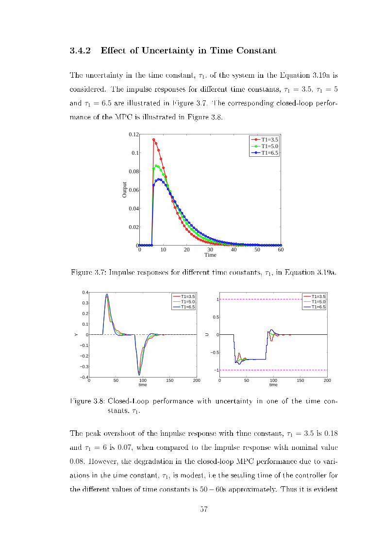
3.4.2 Eect of Uncertainty in Time Constant
The uncertainty in the time constant, τ1, of the system in the Equation 3.19a is
considered. The impulse responses for dierent time constants, τ1 = 3.5, τ1 = 5
and τ1 = 6.5 are illustrated in Figure 3.7. The corresponding closed-loop perfor-
mance of the MPC is illustrated in Figure 3.8.
0 10 20 30 40 50 600
0.02
0.04
0.06
0.08
0.1
0.12
Time
Out
put
T1=3.5T1=5.0T1=6.5
Figure 3.7: Impulse responses for dierent time constants, τ1, in Equation 3.19a.
0 50 100 150 200−0.4
−0.3
−0.2
−0.1
0
0.1
0.2
0.3
0.4
time
Y
T1=3.5T1=5.0T1=6.5
0 50 100 150 200
−1
−0.5
0
0.5
1
time
U
T1=3.5T1=5.0T1=6.5
Figure 3.8: Closed-Loop performance with uncertainty in one of the time con-stants, τ1.
The peak overshoot of the impulse response with time constant, τ1 = 3.5 is 0.18
and τ1 = 6 is 0.07, when compared to the impulse response with nominal value
0.08. However, the degradation in the closed-loop MPC performance due to vari-
ations in the time constant, τ1, is modest, i.e the settling time of the controller for
the dierent values of time constants is 50−60s approximately. Thus it is evident
57

that the closed loop performance of the controller with varying time constants are
almost equal.
3.4.3 Eect of Uncertainty in zero β
The impulse responses for dierent values of β are illustrated in Figure 3.9. This is
related to an uncertainty in the zero of the system. It is evident that the impulse
response with β = 4 is 0.15 which is much more dierent from the nominal impulse
response (β = 2) where amplitude of the response is 0.08. The impulse response
with β = 0 is 0.07 which is much closer to nominal response. From Figure 3.10, it
is seen that β = 0 has higher overshoot of 0.35 when compared with β = 4 where
amplitude is 0.25, but has lesser oscillations and settles with a settling time of
75. It is evident from Figure 3.10, the closed loop performance for the case β = 4
becomes oscillatory and variations in U are quite high when compared with the
performance of the controller having β = 0.
0 10 20 30 40 50 600
0.02
0.04
0.06
0.08
0.1
0.12
0.14
0.16
Time
Out
put
Beta=0Beta=2.0Beta=4
Figure 3.9: Impulse responses for dierent values of β in (3.19a).
3.4.4 Eect of Uncertainty in Time Delay
The eect of variations in the time delay, τ , of Equation 3.19a on the impulse
responses is illustrated in Figure 3.11. The nominal value of time delay is τ = 5.0
and the time delay considered in plant model are τ = 3.0 and τ = 7.0. The
58

0 50 100 150 200−0.5
0
0.5
time
Y
Beta=0Beta=2.0Beta=4
0 50 100 150 200
−1
−0.5
0
0.5
1
time
U
Beta=0Beta=2.0Beta=4
Figure 3.10: Closed-loop MPC response for uncertain values of zero β in the plant(3.19a).
peak amplitude of the impulse response are shifted horizontally which occurs ar
dierent time instants. However, the closed loop response degrades considerably
with τ = 3.0 and τ = 7.0, as both the responses reach sustained oscillations when
compared with nominal delay. Accordingly, this situation with variations in the
time delay corresponds to signicant impulse response uncertainty.
0 10 20 30 40 50 600
0.01
0.02
0.03
0.04
0.05
0.06
0.07
0.08
0.09
Time
Out
put
Delay=3.0Delay=5.0Delay=7.0
Figure 3.11: Impulse responses for dierent time delays, τ , in Equation 3.19a.
From the variations in impulse response coecients it is seen that the degradation
of the closed-loop MPC performance is signicant as shown in Figure 3.12. The
controller response becomes oscillatory when the uncertainty in the time delay of
the system becomes more than 40 % of the nominal value and the actuator reaches
sustained oscillations and even with τ = 3.0, it reaches the saturation limit.
59

0 50 100 150 200−0.5
0
0.5
time
Y
Delay=3.0Delay=5.0Delay=7.0
0 50 100 150 200
−1
−0.5
0
0.5
1
time
U
Delay=3.0Delay=5.0Delay=7.0
Figure 3.12: Closed-loop MPC performance for uncertainties in plant time delays.
Thus it can be seen that the uncertainty of the impulse response coecients are
well suited to measure the resulting closed-loop MPC performance degradation.
3.4.5 Eect of Measurement Noise and Process Noise
The eect of process noise and measurement noise as well as model uncertainty
on the closed-loop MPC performance is investigated in this section.
0 20 40 60 80 100 120 140 160 180 200−0.4
−0.2
0
0.2
0.4
0.6
0.8
1
D
0 20 40 60 80 100 120 140 160 180 200−0.2
−0.1
0
0.1
0.2
0.3
V
time
Figure 3.13: Top: Deterministic disturbance function(D) with added process noise.Bottom: Measurement noise(v).
It is assumed that the process noise enters the system in the same way as the
unmeasured disturbance, i.e. G = Bd. The simulations in this section are based
on the process noise and measurement noise illustrated in Figure 3.13. The signals
are generated using a process noise variance of Q = 0.012 and a measurement noise
60

0 20 40 60 80 100 120 140 160 180 200−0.6
−0.4
−0.2
0
0.2
0.4
0.6
Y
0 20 40 60 80 100 120 140 160 180 200
−1
−0.5
0
0.5
1
U
time
Figure 3.14: Closed-loop MPC performance for the nominal system - Stochas-tic Case, Top: Output with noise (blue) and Filtered value of out-put(green).
0 20 40 60 80 100 120 140 160 180 200−0.6
−0.4
−0.2
0
0.2
0.4
0.6
Y
0 20 40 60 80 100 120 140 160 180 200
−1
−0.5
0
0.5
1
U
time
Figure 3.15: Closed-loop MPC performance with plant gain K = 1.5 comparedto nominal gain K = 1.0 with noise included in the process, Top:Output with noise (blue) and Filtered value of output (green).
variance of R = 0.0052. The steady state (x0 = 0) is used as the initial state for
the simulations.
The closed-loop MPC performance in the case, when the process model equals the
nominal model used for controller design is illustrated in Figure 3.14. Obviously,
the performance is degraded compared to the deterministic case. As is evident in
Figure 3.15, the closed-loop performance degrades and becomes quite oscillatory
in the case when there is a gain mismatch (K = 1.5). This is because of the
actuator reactions for smaller variations in the output which is actually because
of the noise present in the system and when the plant gain becomes 1.5 times
61

0 20 40 60 80 100 120 140 160 180 200−0.6
−0.4
−0.2
0
0.2
0.4
0.6
Y
0 20 40 60 80 100 120 140 160 180 200
−1
−0.5
0
0.5
1
U
time
Figure 3.16: Closed-loop MPC performance for τ1 = 6.5 with noise included in theprocess (nominal value τ1 = 5), Top: Output with noise (blue) andFiltered value of output (green).
greater than the controller gain, the performance of the controller still degrades
and becomes unstable.
0 20 40 60 80 100 120 140 160 180 200−0.6
−0.4
−0.2
0
0.2
0.4
0.6
Y
0 20 40 60 80 100 120 140 160 180 200
−1
−0.5
0
0.5
1
U
time
Figure 3.17: Closed-loop MPC performance for β = 4 with noise included in theprocess (nominal value β = 2), Top: Output with noise (blue) andFiltered value of output (green).
The eect of a time constant mismatch (τ1 = 6.5) is illustrated in Figure 3.16.
In this case the performance degradation compared to the nominal case is less
pronounced. Thus the closed loop performance does not degrade signicantly
with uncertainty in time constant as in the deterministic case but the controller
provides variation in the actuator because of the noise present in the process.
As provided in Figure 3.17, the closed-loop response degrades signicantly and
62
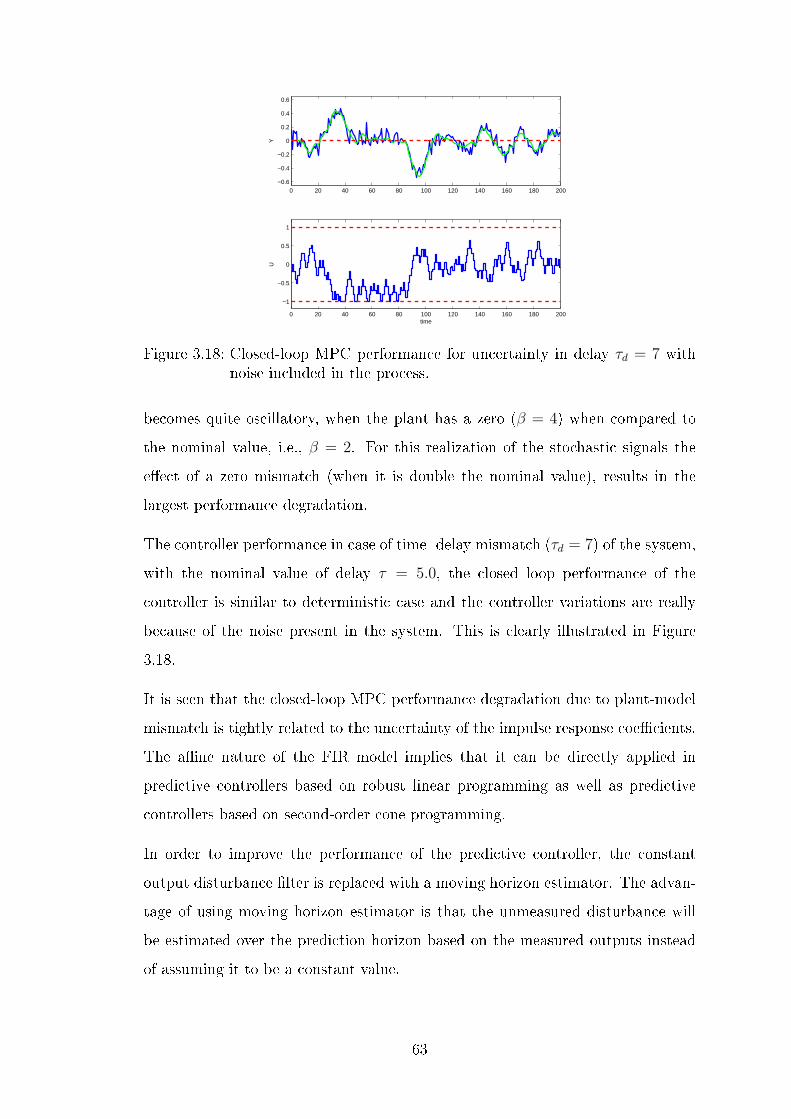
0 20 40 60 80 100 120 140 160 180 200−0.6
−0.4
−0.2
0
0.2
0.4
0.6
Y
0 20 40 60 80 100 120 140 160 180 200
−1
−0.5
0
0.5
1
U
time
Figure 3.18: Closed-loop MPC performance for uncertainty in delay τd = 7 withnoise included in the process.
becomes quite oscillatory, when the plant has a zero (β = 4) when compared to
the nominal value, i.e., β = 2. For this realization of the stochastic signals the
eect of a zero mismatch (when it is double the nominal value), results in the
largest performance degradation.
The controller performance in case of time- delay mismatch (τd = 7) of the system,
with the nominal value of delay τ = 5.0, the closed loop performance of the
controller is similar to deterministic case and the controller variations are really
because of the noise present in the system. This is clearly illustrated in Figure
3.18.
It is seen that the closed-loop MPC performance degradation due to plant-model
mismatch is tightly related to the uncertainty of the impulse response coecients.
The ane nature of the FIR model implies that it can be directly applied in
predictive controllers based on robust linear programming as well as predictive
controllers based on second-order cone programming.
In order to improve the performance of the predictive controller, the constant
output disturbance lter is replaced with a moving horizon estimator. The advan-
tage of using moving horizon estimator is that the unmeasured disturbance will
be estimated over the prediction horizon based on the measured outputs instead
of assuming it to be a constant value.
63

3.5 Moving Horizon Estimation
Figure 3.19 illustrates the estimation and regulation problem.The estimator must
select a disturbance sequence such that historical measurements are reconciled,
while regulator must select manipulated variables such that the distance of the
predicted outputs to the set-points is minimized. This control law is implemented
in a moving horizon such that only the rst MV in this sequence is implemented
on the plant. At the next sample time the procedure is repeated.
Figure 3.19: Moving horizon estimation and regulation.
3.5.1 Model used by Regulator and Estimator
The plant and sensors are assumed as in section 3.3 to be a linear state space
system. The model used in the estimation problem is a nite impulse response
(FIR) model
zk = bk +n∑
i=1
Hu,iuk−i +n∑
i=0
Hd,idk−i (3.13)
in which Hu,ini=1 are the impulse response coecients from the manipulated
variables(or known process inputs) to the outputs, while Hd,ini=0 are the impulse
response coecients from the unknown process disturbances denoted by dk. The
process disturbances, dk, are assumed to consist of a deterministic and a stochastic
component, i.e. dk =[d′k w′
k
]′. It is assumed that there is no immediate eect
from the control inputs to the outputs, i.e. Hu,0 = 0. In contrast, the unknown
disturbances may have a direct inuence on the outputs i.e. in general Hd,0 = 0.
64

This parametrization allows unknown input as well as output disturbances. bk is
the bias term that may be used to account for the mean of zk.
In this work, the moving horizon estimator is based on the FIR model as in Equa-
tion 3.13. The simple estimator in section (3.3.3) used by the model predictive
controller in the previous chapter, is replaced by the following set of equations,
the controller part of the calculation is similar to Equation 3.6a.
minz,d
ϕ =1
2
Ne∑k=0
∥zk − yk∥2Qz+ ∥∆dk∥2S + ∥dk∥2R (3.14a)
s.t. zk = bk +n∑
i=0
Hd,idk−i (3.14b)
dmin ≤ dk ≤ dmax k = 0, . . . , Ne (3.14c)
∆dmin ≤ ∆dk ≤ ∆dmax k = 0, . . . , Ne (3.14d)
where bk = bk +n∑
i=1
Hu,iuk−i k = 1, . . . , Ne (3.14e)
It is assumed that di−ni=−1 are disturbance values xed at their previous estimates
such that the real decision variables in Equation (3.14e), are dkNe
k=0. The decision
variables are normally split into a slow varying component (level), dk and a rapid
varying component (process noise), wk, thus the unknown disturbance can be
given as dk = dk + wk.
3.5.2 Regulator
For the regulator the current time is indexed as k = 0 as in Figure 3.19. The out-
put predictions used by the regulator are based on the FIR model with the past un-
known disturbances xed at their last estimated values,
dk = dk =
[ˆ ′dk wk
′]′0
k=−Ne
,
and the predicted future disturbances are equal to the estimated current mean dis-
turbance value, i.e.
dk =
[ˆ ′d0 0′
]′Nr
k=1
. This implies that the output prediction
65

in the regulator becomes
zk = bk +n∑
i=1
Hi,uuk−i (3.15)
with
bk = bk +n∑
i=0
Hd,idk−i (3.16)
in which Hini=1 are the impulse response coecients (Markov parameters). bk is
a bias term generated by the estimator. bk accounts for discrepancies between the
predicted output and the actual output. In this paper, the output predictions used
by the regulator are based on the FIR model as in Equation (3.15). Consequently,
using the FIR model in Equation (3.15), the regularized l2 output tracking problem
with input constraints may be formulated as
minz,u
ϕ =1
2
Nr−1∑k=0
∥zk+1 − rk+1∥2Qz+ ∥∆uk∥2S (3.17a)
s.t. zk = bk +n∑
i=1
Hiuk−i k = 1, . . . , N (3.17b)
umin ≤ uk ≤ umax k = 0, . . . , N − 1 (3.17c)
∆umin ≤ ∆uk ≤ ∆umax k = 0, . . . , N − 1 (3.17d)
in which∆uk = uk−uk−1. Here we are more concerned with the design of estimator
rather than a regulator, so we adopt a standard approach for formulation of moving
horizon estimation as in Appendix A.2.
3.6 Simulation
In this Section the plants are considered of the form
Z(s) = Y (s) = G(s)U(s) +Gd(s)D(s) (3.18)
66

with the transfer functions
G(s) =K(βs+ 1)
(τ1s+ 1)(τ2s+ 1)e−τs (3.19a)
(3.19b)
Gd(s) =Kd(βds+ 1)
(τd1s+ 1)(τd2s+ 1)e−τds (3.19c)
The disturbance model, Gd(s), is kept xed at its nominal value, while the transfer
function, G(s), from U(s) varies around its nominal value. This is used to illustrate
the consequence of model uncertainty on the MPC closed-loop performance. The
nominal system considered here is K = Kd = 1, τ1 = τ2 = τd1 = τd2 = 5,
β = βd = 2, and τ = τd = 5. The system is converted to discrete time using
a sample time of Ts = 1 and a zero-order-hold assumption on the inputs and
corrupted by normally distributed measurement noise.
y(tk) = z(tk) + v(tk)v(tk) ∼ Niid(0, r2) (3.20)
The nominal model used by estimator and regulator is
Z(s) = G(s)U(s) + Gd(s)(D(s) +W (s)) (3.21)
with G(s) = G(s) and Gd(s) = Gd(s) for the nominal parameters.
Here the performance of regulator is evaluated with MHE by introducing an un-
known step disturbance and try to estimate the disturbance and use it as a feed
back to the MPC. The output are measured at discrete times ( Sample Interval
Ts = 1 ) and corrupted by normally distributed measurement noise.
The constraint limits are dmin = −10, dmax = 10, ∆dmin = −1, ∆dmax = 1,
wmin = −0.5, wmax = 0.5, ∆wmin = −2 and ∆wmax = 2. The horizon of the FIR
model is n = 50 and the estimation window has size Ne = 200.
A. Batch Estimation :
In batch estimation, the outputs are generated by disturbance scenario. The
67

manipulated inputs are zero in this scenario. The disturbance is given as step
up and step down, this disturbance is unknown to the estimator. The measured
outputs are corrupted by measurement noise.
0 50 100 150 200−0.2
0
0.2
0.4
0.6
0.8
Out
put
0 50 100 150 200−0.2
0
0.2
0.4
0.6
0.8
Dis
turb
ance
Time
Figure 3.20: Batch estimation with no measurement noise. Top: Measured Out-put Bottom: Actual and Estimated disturbance Low regularizationweights (Sd = 0.1 and Rw = 0.01).
0 50 100 150 200−0.5
0
0.5
1
Out
put
0 50 100 150 200−1
−0.5
0
0.5
1
1.5
Dis
turb
ance
Time
Figure 3.21: Batch estimation with measurement noise and (Sd = 0.1 , Rw =0.01). Top: Measured Output Z (solid line)and Output with noise Y(Dots). Bottom: Actual Disturbance (Dotted lines), the estimateddeterministic disturbance(blue) and the total disturbance(with thestochastic component added)(green).
In Figure 3.20, the upper plot is the measured output Z (solid line) and output with
measurement noise Y(dots), generated by the unknown disturbance. The lower
plot is the actual disturbance(red dotted line) and the estimated disturbance(blue
solid line). In the simulation of stochastic disturbance, it is considered that the
68

measured output is corrupted by normally distributed measurement noise that
has a standard deviation, r = 0.2. The most important tuning parameters in the
estimator are the regularization weights Sd and Rw.
0 50 100 150 200−0.5
0
0.5
1
1.5
Out
put
0 50 100 150 200−2
−1
0
1
2
Dis
turb
ance
Time
Figure 3.22: Batch estimation with measurement noise. Medium regularizationweights (Sd = 1 and Rw = 0.1), (Legends : As in Figure 3.21).
0 50 100 150 200−0.5
0
0.5
1
1.5
Out
put
0 50 100 150 200−1
−0.5
0
0.5
1
Dis
turb
ance
Time
Figure 3.23: Batch estimation with measurement noise. High regularizationweights (Sd = 5 and Rw = 0.5), (Legends : As in Figure 3.21).
The task of the estimator is to reconstruct the unknown disturbance, D, from the
measured outputs. It can also be called as the smoother. In case of the system with
no measurement noise, the estimated disturbance can be reconstructed arbitrarily
accurately by lowering the regularization weights. This is illustrated in Figure
3.20. Figure 3.21 provides the details of both deterministic component of the
estimated disturbance and the sum of the estimated deterministic and stochastic
component. The blue curve in the lower part of the gure is the deterministic
69

component of the estimated disturbance and the green curve is the sum of the
estimated and stochastic disturbance.
From Figures 3.21, 3.22 and 3.23, it can be noted that the inclusion of measure-
ment noise disturbs the estimation to a large extent. It can be seen that with lower
regularization the variations of the estimated unknown disturbance exactly follows
the measurement noise. In the Figure it can be seen that the measurement noise
has a standard deviation r = 0.2 and with low regularization the standard devia-
tion of estimated disturbance is 0.18. The frequency variations in the estimated
disturbance components can be attenuated only by increasing the regularization
weights in the estimation as shown in Figures 3.21- 3.23. But the increase in
regularization will aect the estimator performance.
B. Moving Horizon Estimation:
When the estimator in Equation A.13, is implemented in a moving horizon manner
for the unknown disturbance with the inclusion of measurement noise that has a
standard deviation r = 0.2, the result illustrated in Figure 3.24 is obtained.
0 50 100 150 200−1
−0.5
0
0.5
1
1.5
Out
put
0 50 100 150 200−2
−1
0
1
2
Time
Dis
turb
ance
Figure 3.24: Moving Horizon Estimation with measurement noise (r = 0.2) and(Sd = 1 and Rw = 0.1), (Legends : As in Figure 3.21)
By increasing the regularization weights, high frequency variations in the esti-
mated disturbance is attenuated. But this will result in the slower adjustment
in estimating the deterministic change in the real disturbance. The estimated
disturbance lags the real disturbance due to the time delay in the model. Thus
it is seen from the gures that by determining the proper regularization weights
70

on the parameters a better disturbance estimate can be provided. This estimated
disturbance can then be used as a feed back to the regulator.
C. Closed Loop Simulation:
Let Qz = 1, S = 0.1, umin = −1, umax = 1, ∆umin = −0.2, ∆umax = 0.2 and Nr =
200 in the predictive regulator. The closed loop performance of MPC with moving
horizon estimator is shown in Figures 3.26 - 3.28. Figure 3.25 shows the response
obtained in the case of no measurement noise. This response illustrates the ideal
behavior of the system. In particular, the achievable estimated disturbance. The
actuator variations in the controller are also quite smoother but still provides
delayed settling time because of the time delay in the model.
0 50 100 150 200−0.5
0
0.5
Out
put
0 50 100 150 200−1
0
1
Inpu
t (M
V)
0 50 100 150 200−0.5
0
0.5
1
Time
Dis
turb
ance
Figure 3.25: Closed-loop MPC simulation without measurement noise. Bottom:Actual disturbance (red dotted line) and the estimated disturbance(blue). Regularization (Sd = 0.1 and Rw = 0.01).
As a case study, the closed loop performance of the estimator is analyzed when
MHE is made in closed loop with the MPC with measurement noise. The mea-
surement noise is included with the standard deviation r = 0.2. The performance
of the estimator is investigated with dierent regularization from the objective
function as in Equation A.13. When the regularization weight of the MHE has
been made very low, the estimation just follows the measurement noise and the
actuator reacts following the measurement noise providing real output variations
by manipulating the process input as shown in Figure 3.26. From Figure 3.28,
it is observed that as the regularization weight is increased the estimation does
not follow the measurement noise but the estimation becomes sluggish. Thus the
71

0 50 100 150 200−1
0
1
Out
put
0 50 100 150 200−1
0
1
Inpu
t (M
V)
0 50 100 150 200−2
0
2
Time
Dis
turb
ance
Figure 3.26: Closed-loop MPC simulation with measurement noise (r = 0.2). Lowregularization (Sd = 0.1 and Rw = 0.01), Legends as in Figure 3.25.
0 50 100 150 200−1
0
1
Out
put
0 50 100 150 200−1
0
1
Inpu
t (M
V)
0 50 100 150 200−1
0
1
2
Time
Dis
turb
ance
Figure 3.27: Closed-loop MPC simulation with measurement noise (r = 0.2).Medium regularization (Sd = 1 and Rw = 0.1), Legends as in Figure3.25.
controller manipulates the process input with regards to slower variations in the
disturbances. But the output variations become sluggish, along with variations
because of measurement noise and hence the closed loop performance becomes
poor.
The results obtained from closed loop performance of MPC with MHE show that
the MHE produces non-smooth disturbance estimates upon which the regulator
reacts and introduces real output variations by its manipulation of the process
input. By increasing the regularization weights in the estimator, the introduced
process variations are slightly reduced at the expense of slower disturbance rejec-
72

0 50 100 150 200−1
0
1
Out
put
0 50 100 150 200−1
0
1
Inpu
t (M
V)
0 50 100 150 200−0.5
0
0.5
1
Time
Dis
turb
ance
Figure 3.28: Closed-loop MPC simulation with measurement noise (r = 0.2). Highregularization (Sd = 5 and Rw = 0.5), Legends as in Figure 3.25.
tion. These results indicate that MHE is no panacea to MPC. The improvements
can be made by considering other norms, convex formulations (e.g. l1 or l2 with
dead zone). In an unconstrained case a nite horizon LQG controller can be repre-
sented with an unstructured disturbance model in the present work. For the case
Nr = Ne → ∞ it approaches a stationary LQG controller with an unstructured
disturbance model for oset free control. In the next chapter, in order to improve
the robustness incase of plant-model mismatch, a soft constraint is included in the
predictive controller with a simple estimator. It is assumed that the same results
would be obtained using a state- space model based predictive control system, but
the advantage of FIR based model is that future predictions are governed by past
disturbances, which results in better closed loop performance.
3.7 Soft Constrained MPC
The soft constraints can be used to tune and improve the performance of linear
model predictive control. Specically, the eect of uncertain models on the per-
formance of a regularized l2 model predictive controller with input constraints,
input-rate constraints and soft output constraints is investigated in this chapter.
The estimator used here is simple estimator. The reason for using simple estima-
tion instead of MHE is that, the moving horizon estimator are computationally
73

complex and the algorithm needs to solve both regulation and estimation problem
simultaneously.
Here the objective function of the MPC is similar to that of FIR based MPC, but
it includes quadratic and linear weights on soft output constraints with respect
to the reference parameter along with normal deviation and actuator objective
functions as given below
minz,u,η
ϕ =1
2
N−1∑k=0
∥zk+1 − rk+1∥2Qz+ ∥∆uk∥2S
+N∑k=1
1
2∥ηk∥2Sη
+ s′ηηk (3.22a)
subject to the constraints
zk = bk +n∑
i=1
Hiuk−i k = 1, . . . N (3.22b)
umin ≤ uk ≤ umax k = 0, . . . N − 1 (3.22c)
∆umin ≤ ∆uk ≤ ∆umax k = 0, . . . N − 1 (3.22d)
zk ≤ zmax,k + ηk k = 1, . . . N (3.22e)
zk ≥ zmin,k − ηk k = 1, . . . N (3.22f)
ηk ≥ 0 k = 1, . . . N (3.22g)
in which ∆uk = uk − uk−1 and ηk is the slack for soft limits around the reference
variable. Sη and s′η are weights on the slack variables. The derivation for formu-
lating QP from the Equation 3.22 is given in Appendix A.3. The general form of
the derivation for all the Quadratic program equations is given in Appendix C.
3.7.1 Soft Constraint Principle
The basic principle of soft constraint based MPC is shown in Figure 3.29. This
illustrates the basic stage cost function for ℓ2 model predictive control (conven-
74
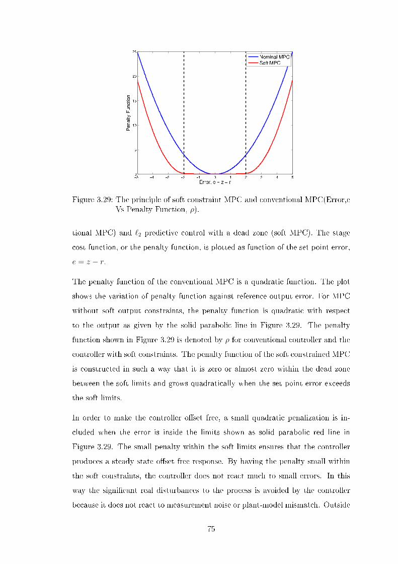
Figure 3.29: The principle of soft constraint MPC and conventional MPC(Error,eVs Penalty Function, ρ).
tional MPC) and ℓ2 predictive control with a dead zone (soft MPC). The stage
cost function, or the penalty function, is plotted as function of the set point error,
e = z − r.
The penalty function of the conventional MPC is a quadratic function. The plot
shows the variation of penalty function against reference output error. For MPC
without soft output constraints, the penalty function is quadratic with respect
to the output as given by the solid parabolic line in Figure 3.29. The penalty
function shown in Figure 3.29 is denoted by ρ for conventional controller and the
controller with soft constraints. The penalty function of the soft constrained MPC
is constructed in such a way that it is zero or almost zero within the dead zone
between the soft limits and grows quadratically when the set point error exceeds
the soft limits.
In order to make the controller oset free, a small quadratic penalization is in-
cluded when the error is inside the limits shown as solid parabolic red line in
Figure 3.29. The small penalty within the soft limits ensures that the controller
produces a steady state oset free response. By having the penalty small within
the soft constraints, the controller does not react much to small errors. In this
way the signicant real disturbances to the process is avoided by the controller
because it does not react to measurement noise or plant-model mismatch. Outside
75

the soft limits, it is assumed that the deviation from target is due to a real process
disturbance, and the soft MPC may be designed to react in the same way as the
conventional MPC. The standard form of Quadratic algorithm for solving the soft
constraint formulation is given in Appendix A.3
The matlab codes for designing a soft MPC and closed loop simulation of the
system in given in Appendix E.
3.7.2 Selection of Soft Limits
The soft output limits considered in the controller is a limit or band around the
reference target of the controlled variable. The performance of the MPC is deter-
mined based on the selection of limits around the reference target. Too wide limit
can cause the controller performance sluggish and even it may lead to steady state
oset. Selecting the soft limits very close to the reference can cause the controller
behave like a conventional MPC and will reduce the robustness of the controller.
Figure 3.30 provides the method for choosing the soft limits. The two curves in
the gure are the linear and quadratic term of the soft constraint. The upper plot
in the gure is the measurement noise over a time horizon and the lower plot is the
response of the linear and quadratic term of the soft constraints for the system
with measurement noise. It is seen from the gure, that the controller almost
rejects the noise and acts only with respect to the process variations.
The soft limits must be selected in a way, such that the controller does not react to
the unnecessary parameter variations because of the measurement noise, process
noise and also the real process variation is considered. In Figure 3.30 it is seen
that for the measurement noise with variance σ2 = 2.5, the soft limits chosen here
is zmax = 2, zmin = −2, so that the controller reacts very less on noise and control
aggressively for real disturbance in the process parameter. Thus the soft limits
must be chosen by considering the variance of the noise (measurement noise as
well as process noise) in the system. In this way the controller can be made to
react only to the real process disturbance and avoid unnecessary actions for the
noise or plant-model mismatch. Thus as a thumb rule it can be dened that when
76

Figure 3.30: Linear (green) and Quadratic term (pink) of the soft constraint.
the variance of the measurement noise in the system σ2 = N . Then the soft limits
to be chosen for the process zmax, zmin must be 0.8− 0.9N . In the next chapter,
the performance of the developed soft MPC is compared with the conventional
MPC to analyze the robustness of the controllers during plant-model mismatch.
3.8 Conclusion
Based on nite impulse response predictions, a regularized l2 predictive controller
with input and input-rate constraints is analyzed. It is veried by simulations
that the closed-loop MPC performance degradation due to plant-model mismatch
is tightly related to the uncertainty of impulse response coecients. The closed
loop performance of the controller is good when the uncertainty in each of the
parameters (separately in gain, zero and time delay) are smaller(upto 40 % incase
of time delay, 50 % in gain and twice incase zero) with the nominal model. The
controller performance reaches sustained oscillations when the uncertainty in each
of these parameters exceeds the above these values. Also presence of noise in
the system further degrades the closed loop performance of the controller. By
MATLAB simulations, the closed loop behavior of moving horizon estimation and
model predictive control for a system with measurement noise is provided. It is
77

evaluated that the closed loop response of the model predictive controller has a
strong correlation to the magnitude of the measurement noise i.e., the quality of
the sensor. However, signicant process variations results from the control systems
due to non-smooth disturbance estimates. These results are not due to the fact
that the regulator and estimator are based on a FIR model.
Then the model predictive controller equipped with soft output constraints along
with input and input - rate constraints is developed. The prediction is based on
the Finite impulse response model, and the feedback is based on simple constant
output disturbance lter.
78
CHAPTER 4
Comparison of Soft MPC with Nominal MPC
Using Simulation
In this chapter, the controllers with and without soft constraints are compared
both for SISO and MIMO cases. By MATLAB simulation, the performance of
the new robust constrained predictive controller is compared with a conventional
predictive controller both in nominal case and in uncertainty conditions. The
model considered here is a SOPDT transfer function model with a zero. It is
assumed that the disturbance in the model enters in the same way as the plant
model. The performance of the controllers with process noise and measurement
noise is also studied.
4.1 Introduction
Model predictive controllers with robust performance against plant-model mis-
match is crucial in long-term maintenance and success of MPC system. Using
soft output constraints in a novel way, it is demonstrated that the poor perfor-
mance of predictive control in the case of plant-model mismatch can be improved
signicantly. The soft constraints create a dead zone around the set point and
by simulation it is demonstrated, that the performance of such an MPC does not
degrade much in the nominal case but improves signicantly in the case of plant-
model mismatch. This technique is similar but not identical to the funnels used
by Honeywell in RMPC (Qin and Badgwell, 2003; Havlena and Lu, 2005; Havlena
and Findejs, 2005). Normally in classical process control, PID control with dead
zones (Shinskey, 1988) have been used in a similar way like soft output constraints
based MPC. The soft output constraint included in the MPC acts as a dead zone
to the controller to reduce its sensitivity to noise and uncertainty when the process
79
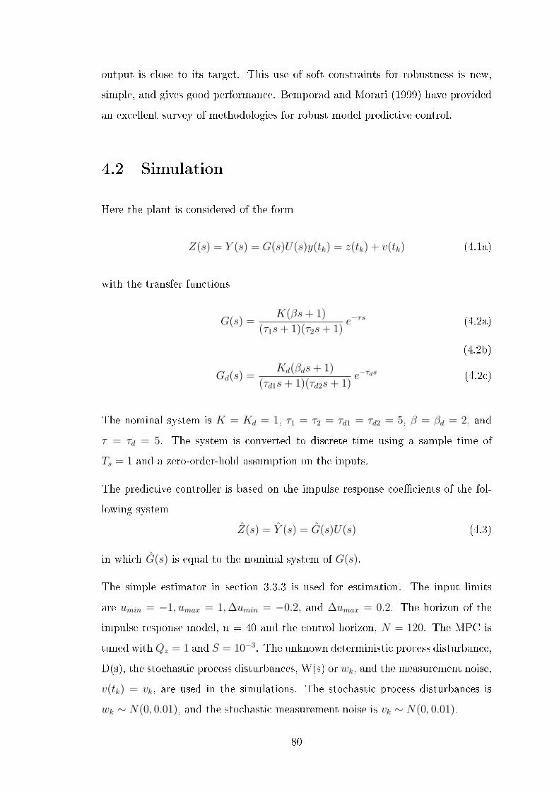
output is close to its target. This use of soft constraints for robustness is new,
simple, and gives good performance. Bemporad and Morari (1999) have provided
an excellent survey of methodologies for robust model predictive control.
4.2 Simulation
Here the plant is considered of the form
Z(s) = Y (s) = G(s)U(s)y(tk) = z(tk) + v(tk) (4.1a)
with the transfer functions
G(s) =K(βs+ 1)
(τ1s+ 1)(τ2s+ 1)e−τs (4.2a)
(4.2b)
Gd(s) =Kd(βds+ 1)
(τd1s+ 1)(τd2s+ 1)e−τds (4.2c)
The nominal system is K = Kd = 1, τ1 = τ2 = τd1 = τd2 = 5, β = βd = 2, and
τ = τd = 5. The system is converted to discrete time using a sample time of
Ts = 1 and a zero-order-hold assumption on the inputs.
The predictive controller is based on the impulse response coecients of the fol-
lowing system
Z(s) = Y (s) = G(s)U(s) (4.3)
in which G(s) is equal to the nominal system of G(s).
The simple estimator in section 3.3.3 is used for estimation. The input limits
are umin = −1, umax = 1,∆umin = −0.2, and ∆umax = 0.2. The horizon of the
impulse response model, n = 40 and the control horizon, N = 120. The MPC is
tuned withQz = 1 and S = 10−3. The unknown deterministic process disturbance,
D(s), the stochastic process disturbances, W(s) or wk, and the measurement noise,
v(tk) = vk, are used in the simulations. The stochastic process disturbances is
wk ∼ N(0, 0.01), and the stochastic measurement noise is vk ∼ N(0, 0.01).
80

4.3 Soft constraints in MPC
A comparison on the performance of the MPC with soft constraints and the con-
ventional MPC is made in deterministic case as well as when the process is per-
turbed by stochastic noises. In cases where noise variance is large, the MPC
without soft constraints reacts to the noise variations resulting in oscillatory per-
formance of the system. So the soft limit is included to penalize heavily only when
it violates the limit and a very little action to drive the output to target with zero
oset within the limit. This way of control relatively gives much stable operation
avoiding unnecessary uctuations in the input.
4.3.1 Eect of including noise in the system
To study the eectiveness of soft constraints, a simple case of second order system
with a zero and input delay is considered as given in Equation (4.2a). The model
used by the controller is identical to the deterministic part of the plant model.
However, the plant has in addition to the deterministic part stochastic process
disturbances and stochastic measurement noise as illustrated in Figure 4.1.
0 50 100 150 200 250 3000
0.5
D
0 50 100 150 200 250 300−0.5
0
0.5
v
0 50 100 150 200 250 300−0.5
0
0.5
w
time
Figure 4.1: External signals used in simulation: Disturbance (dk) measurementnoise (v) and process noise(w).
First, a case is considered, in which the system is perturbed by measurement
noise with variance Qv = 0.01 and process noise with variance Qw = 0.01 and it
is assumed that there is no external disturbance D(s) = 0. The normal weight
81

on measurement error Qz = 0.001 incase of soft MPC and Qz = 1.0 in case of
conventional MPC. The comparison on the open loop performance of MPC for
stochastic system with and without soft constraints is given in Figure 4.2. In
this Figure, the variations of controller input when there is noise in the output is
studied, but the values are not given back to the plant for control actions.
0 50 100 150 200 250 300−1
−0.5
0
0.5
1
Y
0 50 100 150 200 250 300
−1
−0.5
0
0.5
1
U
time
Figure 4.2: Comparison of Open loop performance of conventional and softMPC,with nominal models applied to a stochastic system with nodeterministic disturbance (Conventional MPC = blue, Soft MPC =red).
Though the output variations in both the controller are similar, the input varia-
tions shows the MPC without soft constraints acts even for noise variation. Thus
the input variance of the soft MPC is much smaller than the input variance of
the nominal MPC. Due to the low penalties within the soft limits, the soft MPC
does not react to measurement noise and do not need to compensate such previous
erroneous measurement noise induced input moves. The closed loop performance
further degrades when there is a plant-model mismatch. Further, this can be illus-
trated clearly the system is simulated with plant-model mismatch to be discussed
in the following sections.
4.4 Eect of uncertainties in the model
A deterministic system without process noise or measurement noise is considered.
However, the model used by the controllers is dierent from the plant model. The
82

process is perturbed by an unknown deterministic disturbance, D(s), as illustrated
in Figure 4.1. The performance of the conventional MPC and the soft MPC
for model-plant mismatches dened by the time delay, τd, the gain K, the time
constant τ1, and the zero β are compared.
4.4.1 Eect of uncertainty in Delay
The eect of uncertainty in Delay τd is considered for comparing the performances
of conventional MPC and soft MPC. The performance of both the MPCs and
their corresponding input variations for the deterministic case are illustrated in
Figure 4.3 and Figure 4.4. When the delay τd of the plant model varies with the
controller model there is a reasonable performance degradation in the close loop
control. Here when the plant delay is either higher or lower than the model delay,
it aects the performance considerably.
0 50 100 150 200 250 300−0.4
−0.2
0
0.2
0.4
Y
0 50 100 150 200 250 300
−1
−0.5
0
0.5
1
U
time
Figure 4.3: Closed-loop MPC performance with uncertainty in time delay, τd = 3,in Equation (4.2a)(Conventional MPC = blue, Soft MPC = red).
The uncertainty in time delay, τd = 3.0 and τd = 7.0 is considered here. It
can be seen that when compared to the controller variations with nominal delay
τd = 5.0 the MPC without soft constraints manipulates the control input for small
variations in output, resulting in instability, where as soft MPC does not react to
the small output variations resulting in faster stabilization. It can be seen that
in case of soft MPC, the controller settles within a period of 30s where as the
83

conventional MPC results in sustained oscillations.
0 50 100 150 200 250 300−0.4
−0.2
0
0.2
0.4
Y
0 50 100 150 200 250 300
−1
−0.5
0
0.5
1
U
time
Figure 4.4: Closed-loop MPC performance with higher plant time delay , τd = 7,in Equation (4.2a)(Conventional MPC = blue, Soft MPC = red).
4.4.2 Eect of uncertainty in gain
The eect of uncertainty in the gain, K is considered. The comparison on the
performance of both the MPCs and their corresponding input variations for the
deterministic case is illustrated in Figure 4.5.
When the gain of the process is on the higher side, i.e., K = 2 or more when
compared with the controller model gain K = 1 the closed loop performance of
MPC without soft constraints degrades as it starts acting to variations in output
aggressively, resulting in sustained oscillations. This again makes the output os-
cillatory as shown in the Figure 4.5. But in case of soft MPC the controller does
not react to small variations within the soft limits providing better stability. Here
even the soft MPC has output variations getting oscillatory but settles faster (in
60s) , whereas MPC without soft constraints oscillates the manipulated variable
continuously resulting in continuous oscillations. Incase of plant gain on the lower
side or slightly higher than the controller model gain, the controller will normally
behave sluggish both in conventional MPC and soft MPC, so both the controllers
behave in similar way resulting in stable operation.
84

0 50 100 150 200 250 300−1
−0.5
0
0.5
1
Y
0 50 100 150 200 250 300
−1
−0.5
0
0.5
1
U
time
Figure 4.5: Closed-loop MPC performance with gain uncertainty, K = 2, in Equa-tion (4.2a)(Conventional MPC = blue, Soft MPC = red).
4.4.3 Eect of uncertainty in Time Constant
In case of uncertainty in time constant, τ1 of the system.
When one of the time constants of the system, τ = 2.0 or less when compared to
the nominal time constant τ = 5, the output performance degrades as the input
starts reacting to the variations resulting in sustained oscillations. As referred in
chapter 4, the eect of time constant in all the other cases will remain same as
they do not have signicant impact on the stability.
0 50 100 150 200 250 300−1
−0.5
0
0.5
Y
0 50 100 150 200 250 300
−1
−0.5
0
0.5
1
U
time
Figure 4.6: Closed-loop MPC performance with uncertain time constant, τ1, inEquation (4.2a)(Conventional MPC = blue, Soft MPC = red).
85

The comparison on performance of both the MPCs with the uncertainty in time
constant is illustrated in Figure 4.6. It can be seen that when the time constant
of the plant is close to the sampling time i.e., 2s or less the controller performance
degrades in case of conventional MPC as it provides continuous oscillations, but
soft MPC provides stable variation even with time constants closer to the sampling
time.
4.4.4 Eect of uncertainty in Zero
The uncertainty in the zero β of the system is considered as given in the Figure
4.7.
The plant having the value of zero β = 4.5 or more when considered with nominal
model β = 2 the performance of the conventional MPC degrades with increased
oscillation in the output, where as the soft MPC performs in a much stabilized
way as shown. This behavior is almost similar to that of the uncertain gain model,
but soft MPC settles much faster in this case (settling time of 40s).
0 50 100 150 200 250 300−0.5
0
0.5
Y
0 50 100 150 200 250 300
−1
−0.5
0
0.5
1
U
time
Figure 4.7: Closed-loop MPC performance with uncertain zero, β, in Equation(4.2a)(Conventional MPC = blue, Soft MPC = red).
In all of these cases only the deterministic part of the process is considered, the
closed loop performance can be aected considerably when process noise and mea-
surement noise are included into the system.
86

4.5 Eect of Process noise and Measurement noise
From the previous section, on comparing the performance of MPC with and with-
out soft output constraints for a deterministic model, it is observed that the un-
certainty in any of the parameters of the model degrades the performance of con-
ventional MPC considerably than the MPC with soft constraints.
The eect of process noise and the measurement noise on the closed loop perfor-
mance is investigated. It is assumed that the process noise enters the same way
as the unmeasured disturbance, i.e. G = Bd.
For simulation purpose, we generate the signals with the process noise variance of
Qw = 0.012 and the measurement noise variance of Qv = 0.012. The steady state
(x0 = 0) is used as the initial state for the simulations.
The closed loop performance of the conventional MPC and the soft MPC is com-
pared with the nominal model and inclusion of the measurement noise . The
closed loop performance is as shown in Figure 4.8. It can be seen that the con-
ventional MPC reacts for small variations in output which is because of the noise
perturbations in the system. This makes the inputs from the controller oscillatory
resulting in unstable operation. In this case, the controlled variable, Y (or Z), of
the two controllers are similar while the manipulated variable, U, of the soft MPC
has signicantly less variance than the manipulated variable, U, of the nominal
MPC.
The closed loop performance of a conventional MPC and a soft MPC applied to
the system with the external signals in Figure 4.1 and a plant-model mismatch in
the gain is compared. The plant gain is K = 2 and the controller gain is K = 1.
As evident in Figure 4.9, the closed-loop performance of the conventional MPC
degrades and becomes quite oscillatory in the case when there is a gain mismatch
(K = 2.0). It is seen that the performance of the soft MPC is signicantly
better than the performance of the conventional MPC. The superior performance
is achieved by having a small set point deviation penalty within the soft constraints
such that the controller does not react aggressively when close to the set point.
87

0 50 100 150 200 250 300−1
−0.5
0
0.5
1
Y
0 50 100 150 200 250 300
−1
−0.5
0
0.5
1
U
time
Figure 4.8: Comparison of normal and soft MPC with nominal models applied toa stochastic system with an unknown deterministic disturbance (Con-ventional MPC = blue, Soft MPC = red).
In this way it avoids perturbing the system due to stochastic measurement noise
and plant-model mismatch.
0 50 100 150 200 250 300−1
0
1
2
Y
0 50 100 150 200 250 300
−1
−0.5
0
0.5
1
U
time
Figure 4.9: Closed-loop MPC performance with noise and gain uncertainty, Theplant gain is K = 2 and the model gain is K = 1(Conventional MPC= blue, Soft MPC = red).
4.6 Simulation of MIMO System
The performance of the controllers for MIMO case is simulated using Matlab. The
model considered here is taken from the cement mill circuit from the chapter 5.4.
88
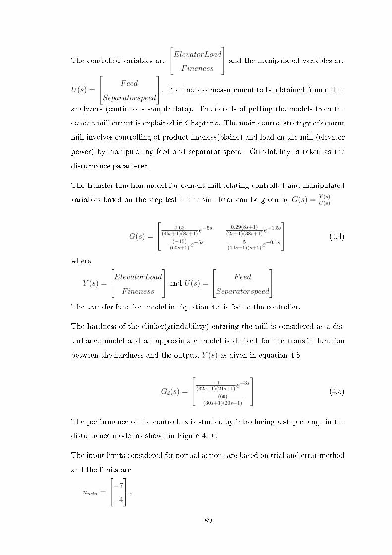
The controlled variables are
ElevatorLoadFineness
and the manipulated variables are
U(s) =
Feed
Separatorspeed
. The neness measurement to be obtained from online
analyzers (continuous sample data). The details of getting the models from the
cement mill circuit is explained in Chapter 5. The main control strategy of cement
mill involves controlling of product neness(blaine) and load on the mill (elevator
power) by manipulating feed and separator speed. Grindability is taken as the
disturbance parameter.
The transfer function model for cement mill relating controlled and manipulated
variables based on the step test in the simulator can be given by G(s) = Y (s)U(s)
G(s) =
0.62(45s+1)(8s+1)
e−5s 0.29(8s+1)(2s+1)(38s+1)
e−1.5s
(−15)(60s+1)
e−5s 5(14s+1)(s+1)
e−0.1s
(4.4)
where
Y (s) =
ElevatorLoadFineness
and U(s) =
Feed
Separatorspeed
The transfer function model in Equation 4.4 is fed to the controller.
The hardness of the clinker(grindability) entering the mill is considered as a dis-
turbance model and an approximate model is derived for the transfer function
between the hardness and the output, Y (s) as given in equation 4.5.
Gd(s) =
−1(32s+1)(21s+1)
e−3s
(60)(30s+1)(20s+1)
(4.5)
The performance of the controllers is studied by introducing a step change in the
disturbance model as shown in Figure 4.10.
The input limits considered for normal actions are based on trial and error method
and the limits are
umin =
−7−4
,89
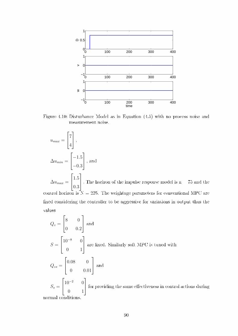
0 100 200 300 4000
0.5
1
D0 100 200 300 400
−1
0
1
v
0 100 200 300 400−1
0
1w
time
Figure 4.10: Disturbance Model as in Equation (4.5) with no process noise andmeasurement noise.
umax =
74
,∆umin =
−1.5−0.3
, and∆umax =
1.50.3
. The horizon of the impulse response model is n = 75 and the
control horizon is N = 225. The weightage parameters for conventional MPC are
xed considering the controller to be aggressive for variations in output thus the
values
Qz =
8 0
0 0.2
and
S =
10−8 0
0 1
are xed. Similarly soft MPC is tuned with
Qzs =
0.08 0
0 0.01
and
Ss =
10−2 0
0 1
for providing the same eectiveness in control actions during
normal conditions.
90

The performance of the conventional MPC is slightly better than the MPC with
soft constraints for nominal cases as shown in Figure 4.11. This is because the
soft MPC does not react aggressively when the outputs are within the soft limits.
0 100 200 300 400−0.5
0
0.5
Y1
0 100 200 300 400−5
0
5
10
Y2
0 100 200 300 400
−5
0
5
U1
0 100 200 300 400−4
−2
0
2
4
U2
time
Figure 4.11: Variation of controllers Nominal Case, as in Equation (4.4) (Conven-tional MPC = blue, Soft MPC = red).
4.6.1 Eect of uncertainty in gain
The cement mill model is simulated using MATLAB by introducing uncertainty
in the model gain using single value decomposition (SVD) method. The original
gain of the system are decomposed using SVD as Gain,
K =
1.6866 1.4240
−14.9812 5.0200
and then fed as a new model to the controller.
The comparison of the controllers with the new gain is given in Figure 4.12. As the
uncertainty in gain increases, the normal controller becomes aggressive resulting
in oscillatory behavior. Since the weight on deviation of Y1 is more than Y2 the
controller reacts more for maintaining the parameter(Y1) resulting in sustained
oscillations, when compared to Y2. In case of soft MPC it can be seen that
both the control parameters settle before 75% of the control horizon resulting
in stable operation. These features are expected to contribute to better closed
loop performance, easier maintenance, easier tuning, and longer lifetime of model
predictive controllers for chemical processes.
In the next chapter, the performance of both the controllers when applied to a
cement mill circuit which is subjected to large number of uncertainties is studied.
91

0 100 200 300 400−0.5
0
0.5
Y1
0 100 200 300 400−5
0
5
10
Y2
0 100 200 300 400
−5
0
5
U1
0 100 200 300 400−4
−2
0
2
4
U2
time
Figure 4.12: Comparison of Conventional MPC and Soft MPC in case of Uncer-tainty in Gain, K (MIMO), in Equation (4.4)(Conventional MPC =blue, Soft MPC = red).
4.7 Conclusion
It is veried by simulations that the soft MPC provides much robust performance
in the face of plant-model mismatch than conventional MPC. In nominal case,
it can be seen that the performance of conventional MPC is slightly better than
the soft MPC. This is because in soft MPC, the controller actions are very small
whenever the error is closer to target(within the soft band) resulting in sluggish
performance. In SISO case with uncertain system, it can be seen that soft MPC
stabilizes the system faster than conventional MPC. The performance of both the
controllers are similar, with the uncertainty condition when the plant gain and
zero is lesser than the controller gain and zero, also with plant having higher time
constant values than the controller model. When there is uncertainty in time delay
(both higher and lower values) of the system the soft MPC settles in 50s. But in
case of uncertainty in gain it can be seen that the soft MPC is little oscillatory
and settles much slower. For the MIMO case, with uncertainty in the model gain,
the conventional MPC results in sustained oscillations where as in soft MPC the
oscillations are suppressed completely and the system settles before 75% of the
control horizon.
92

CHAPTER 5
Cement Manufacturing Process
In this chapter, a brief overview of the cement plant architecture is given, in
which the developed robust MPC is to be implemented. Also the importance of
cement mill operation in the cement plant a and the need for control of cement
mill circuit is discussed. A transfer function model for the cement mill circuit is
developed from the data obtained from the cement mill simulation system through
step response tests. The transfer function of the system is a 2 × 2 system with
Feed rate and separator speed as manipulated variables and Elevator load and
Fineness as controlled variables.
5.1 Introduction
The annual world consumption of cement is around 1.7 billion tonnes and is in-
creasing at about 1% a year. The electrical energy consumed in the cement produc-
tion is approximately 110 kWh/tonne. 30% of the electrical energy is used for raw
material crushing and grinding while around 40% of this energy is consumed for
grinding clinker to cement powder (Fujimoto, 1993; Jankovic et al., 2004). Hence,
global cement production uses 18.7 TWh which is approximately 2% of the worlds
primary energy consumption and 5% of the total industrial energy consumption.
The cement manufacturing process is illustrated in Figure 5.1.
PROCESS DESCRIPTION
Cement industries typically produce portland cement, although they also produce
masonry cement (which is also manufactured at portland cement plants). Portland
cement is a ne, typically gray powder comprised of dicalcium silicate, tricalcium
silicate, tricalcium aluminate, and tetracalcium aluminoferrite, with the addition
of forms of calcium sulfate. Dierent types of portland cements are created based
93

Quary Crusher Transport Mixing bed
Raw Mill
Dust filter
Preheater / calciner
Kiln Clinker cooler
Clinker silo
Cement mill
Cement silos / Packaging
Figure 5.1: Cement plant (FLSmidthA/S (2004)).
on the use and chemical and physical properties desired. Portland cement types
I - V are the most common. Portland cement plants can operate continuously for
long time periods (i.e., 6 months) with minimal shut down time for maintenance.
The air pollution problems related to the production, handling, and transporta-
tion of portland cement are caused by the very ne particles in the product. The
stages of cement production at a portland cement plant are:
a. Procurement of raw materials
b. Raw Milling - preparation of raw materials for the pyroprocessing system
c. Pyroprocessing - pyroprocessing raw materials to form portland cement clinker
d. Cooling of portland cement clinker
e. Storage of portland cement clinker
f. Finish Milling
g. Packing and loading
a. Raw Material Acquisition
Most of the raw materials used are extracted from the earth through mining and
quarrying and can be divided into the following groups: lime (calcareous), silica
(siliceous), alumina (argillaceous), and iron (ferriferous). Since a form of calcium
carbonate, usually limestone, is the predominant raw material, most plants are
situated near a limestone quarry or receive this material from a source via inex-
pensive transportation. The plant must minimize the transportation cost since
one third of the limestone is converted to CO2 during the pyroprocessing and
94

is subsequently lost. Quarry operations consist of drilling, blasting, excavating,
handling, loading, hauling, crushing, screening, stockpiling, and storing.
b. Raw Milling
Raw milling involves mixing the extracted raw materials to obtain the correct
chemical conguration, and grinding them to achieve the proper particle-size to
ensure optimal fuel eciency in the cement kiln and strength in the nal concrete
product. Three types of processes may be used: the dry process, the wet process,
or the semidry process. If the dry process is used, the raw materials are dried
using impact dryers, drum dryers, paddle-equipped rapid dryers, air separators,
or autogenous mills, before grinding, or in the grinding process itself. In the wet
process, water is added during grinding. In the semidry process the materials are
formed into pellets with the addition of water in a pelletizing device.
c. Pyroprocessing
In pyroprocessing, the raw mix is heated to produce portland cement clinkers.
Clinkers are hard, gray, spherical nodules with diameters ranging from 0.32 - 5.0
cm (1/8 - 2") created from the chemical reactions between the raw materials.
The pyroprocessing system involves three steps: drying or preheating, calcining
(a heating process in which calcium oxide is formed), and burning (sintering).
The pyroprocessing takes place in the burning/kiln department. The raw mix
is supplied to the system as a slurry (wet process), a powder (dry process), or
as moist pellets (semidry process). All systems use a rotary kiln and contain
the burning stage and all or part of the calcining stage. For the wet and dry
processes, all pyroprocessing operations take place in the rotary kiln, while drying
and preheating and some of the calcination are performed outside the kiln on
moving grates supplied with hot kiln gases.
d. Clinker Cooling
The clinker cooling operation recovers up to 30% of kiln system heat, preserves
the ideal product qualities, and enables the cooled clinker to be maneuvered by
conveyors. The most common types of clinker coolers are reciprocating grate,
planetary, and rotary. Air sent through the clinker to cool it is directed to the ro-
95

tary kiln where it nourishes fuel combustion. The fairly coarse dust collected from
clinker coolers is comprised of cement minerals and is restored to the operation.
Based on the cooling eciency and desired cooled temperature, the amount of air
used in this cooling process is approximately 1-2 kg/kg of clinker. The amount of
gas to be cleaned following the cooling process is decreased when a portion of the
gas is used for other processes such as coal drying.
e. Clinker Storage
Although clinker storage capacity is based on the state of the market, a plant can
normally store 5 - 25% of its annual clinker production capacity. Equipment such
as conveyors and bucket elevators is used to transfer the clinkers from coolers to
storage areas and to the nish mill. Gravity drops and transfer points typically
are vented to dust collectors.
f. Finish Milling
During the nal stage of portland cement production known as nish milling, the
clinker is ground with other materials (which impart special characteristics to the
nished product) into a ne powder. Up to 5% gypsum and/or natural anhydrite
is added to regulate the setting time of the cement. Other chemicals, such as
those which regulate ow or air entrainment, may also be added. Many plants use
a roll crusher to achieve a preliminary size reduction of the clinker and gypsum.
These materials are then sent through ball or tube mills (rotating, horizontal steel
cylinders containing steel alloy balls) which perform the remaining grinding. The
grinding process occurs in a closed system with an air separator that divides the
cement particles according to size. Material that has not been completely ground
is sent through the system again.
g. Packing and Loading
Once the production of portland cement is complete, the nished product is trans-
ferred using bucket elevators and conveyors to large, storage silos in the shipping
department. Most of the portland cement is transported in bulk by railway, truck,
or barge, or in 43 kg (94 pound) multiwalled paper bags. Bags are used primarily
to package masonry cement. Once the cement leaves the plant, distribution ter-
96

Figure 5.2: Cement mill grinding circuit (FLSmidthA/S (2004)).
minals are sometimes used as an intermediary holding location prior to customer
distribution. The same types of conveyor systems used at the plant are used to
load cement at distribution terminals.
5.2 Cement Ball Mill Process
The nish milling circuit consumes signicant amounts of energy: throughput is
high (generally in the range 120 t/h to 150 t/h) and the target particle size is
relatively ne. Typically, nished cement is produced using ceramic ball mills,
although roller mills are becoming increasingly popular. With either mill it is
common for a dynamic separator to take a ne product cut, coarse material being
recycled to the mill for further grinding.
Figure 5.2 illustrates a rotating cement ball mill in a closed loop with a separator.
The ball mills used for grinding cement have usually two chambers separated by
a metallic diaphragm as shown in Figure 5.3. The rst compartment is lled
with bigger balls and lifting liners and is supposed to do coarse grinding. The
second compartment is the ne grinding chamber and is equipped with a smaller
ball charge and classifying liners. Classifying liners ensure, that the ball charge is
segregated and bigger balls accumulate at the beginning of the compartment and
smaller balls toward the end. The feed materials (Clinker,Gypsum and Fly Ash)
are fed to the rst chamber of the mill where they are broken into smaller powder
by the impact of falling balls. Then the particles pass through metallic diaphragm
97

Mill inlet
Mill discharge
Ball filling 2. compartment
Ball filling 1. compartment
Drive
Intermediate diaphragm
Discharge diaphragm
Figure 5.3: Ball mill(FLSmidthA/S (2004)).
into the second chamber. The second chamber consists of much smaller balls for
making the particles ner.
The ne ground particles are then lifted by a bucket elevator and sent to a air
classier shown in Figure 5.4. A classier is essential to the clicker grinding process
in order to remove coarse particles, which require further grinding, from the ne
particles, which meet specication.
In the classier, the milled powder is suspended in the air stream. Air is sucked
from the bottom of the classier forcing coarse particles impact on the walls of
the classier. These coarse particles can then be collected as they drop down due
to gravity through cone shaped cyclones; whereas nes particles are transported
away in the air stream towards the center of the classier. The rejects are then
recirculated to the mill for further grinding. The ner particles then are collected
as nal product in cement silos. The classier and the ball mill eciency can
be improved by maintaining a constant recirculation ratio (rejects to main feed
ratio), which in-turn provide a consistent product quality.
5.2.1 Tromp Curves
The eciency of a classier must be determined to make sure that no oversized
particles are present in the nal product and that ne particles are not processed
98

Figure 5.4: Classier(FLSmidthA/S (2004)).
any further. This can be measured by plotting Tromp curves as shown in Figure
5.5. These plots show the probability that a particle of a particular size is sepa-
rated into coarse (overow) fraction. Exact critical examination of the classier
eciency (sharpness of separation) takes place on the basis of the Tromp curve.
This curve is calculated from the percentages by weight of the individual grain
size fractions in the three classier material ows: feed, tailings and nes. The
result of the calculation is a selectivity factor (weight by %) for a specic grain
fraction. From the entered quantity of points, the function shown in the diagram:
"selectivity factor (%) as a function of the grain size (m)" is obtained.
5.3 Cement Mill Control Strategy
The ball mill control is considered to be a very dicult control problem. The main
reason for this is the presence of non-linearities and uncertainties in the system.
The model predictive control without soft constraints is more eective when the
plant model matches with the controller model. Physical and chemical properties
99

Figure 5.5: Tromp Curve(FLSmidthA/S (2004)).
of the raw material, mechanical wear and tear and various other factors deterio-
rates the model in long run. This model mismatch is considered for designing a
controller which neglects the small variations and acts only to the large process
disturbances. Stabilizing cement ball mill involves maintaining load on the mill
and the neness of the product. The mill loading can be represented by dier-
ent parameters like Sound inside the mill created by collision of metal balls, mill
main motor drive power and bucket elevator power. Normally elevator power is
considered as the most reliable parameter as it indicates exact amount of ground
material coming out of the mill. The amount of feed entering the mill and classi-
er speed for separating the ne and coarse particles are varied for controlling the
above parameters.
5.4 Cement Mill Model
The transfer function model for cement mill relating controlled and manipulated
variables is obtained using a simulation software called ECS/CEMulator. The
ECS/CEMulator, reects most of the real time conditions and hence the model
100

can be considered to match a real plant. A detailed description of CEMulator
is given in Appendix F. The models are obtained by varying the manipulated
variables in step and observe the variations of controlled variables with respect
to the step change. Dierent step sizes in each of the manipulated variables are
given in order to get the exact impact on the controlled variables on the actuators.
Also the variations in the controlled variables are obtained for dierent step sizes
of Feed and Separator speed in the CEMulator as given in Figures 5.6 and 5.7.
In the gure it can be seen that the step disturbances on Feed rate and Elevator
load are given in both the directions with 5 % and 10 % variations and also for
dierent operating conditions (Grindability of 28 and 36).
5.4.1 Step Test Procedure
The test procedures specied in the following sections describes the experiments
needed obtain the data used for construction of a nite impulse response (FIR)
model. Ideally, a model should be established for each operating point
The general principle in the model construction phase is to stabilize the system
around its desired operating point and then perturb the system with a step change
of each of the process inputs. The responses of the output (measurement) variables
are recorded. The process inputs must be perturbed individually. By the data
obtained by this procedure a model describing the inuence of the process inputs
on the process outputs can be constructed. The controller uses this model for
computation of the control actions
The cement mill has to process inputs that must be perturbed. The fresh feed
ow rate and the separator speed. In principle all possible variables should be
recorded. Of particular importance are the Blaine (or residue, on-line as well
as lab measurements), Folaphone, Elevator Power (or current), Mill Power and
Reject Flow Rate as given in Table 5.1.
Based on these step response results an approximate model is identied, by plot-
ting a step response curve with the transfer function models in the MATLAB as
shown in Figure 5.8.
101

0 20 40 60 80 100 120 140 160 180 200−0.1
0
0.1
0.2
0.3
0.4
0.5
0.6
0.7Feed Vs Elev
time
Ste
pCoe
ff
10%−5%5%−10%10%(G28)−10%(G28)5%(G36)−5%(G36)
0 20 40 60 80 100 120 140 160 180 200−16
−14
−12
−10
−8
−6
−4
−2
0
2Feed Vs Fine
time
Ste
pCoe
ff
10%−5%5%−10%10%(G28)−10%(G28)5%(G36)−5%(G36)
Figure 5.6: Step Response results for dierent operating conditions(dierentGrindability factors ) and with dierent step sizes of Feed(+5 %, -5 % ..).
102

0 20 40 60 80 100 120 140 160 180 200−0.05
0
0.05
0.1
0.15
0.2
0.25
0.3
0.35Sep Vs Elev
time
Ste
pCoe
ff
10%−5%5%−10%10%(G28)−10%(G28)5%(G36)−5%(G36)
0 20 40 60 80 100 120 140 160 180 200−2
0
2
4
6
8
10
12
14Sep Vs Fine
time
Ste
pCoe
ff
10%−5%5%−10%10%(G28)−10%(G28)5%(G36)−5%(G36)
Figure 5.7: Step Response results for dierent operating conditions(dierentGrindability factors ) and with dierent step sizes of Separator(+5%, -5 % ..).
103

0 20 40 60 80 100 120 140121
122
123
124
125
126
127
Fee
d R
ate
time (hours)
FeedRate vs Elevator Load
0 20 40 60 80 100 120 14024
24.5
25
25.5
26
26.5
27
time (hours)
Ele
vato
r Lo
ad
MeasurementTrial
0 20 40 60 80 100 120 140126
128
130
132
134
136
Fee
d R
ate
time (hours)
FeedRate vs Fineness
0 20 40 60 80 100 120 1403000
3050
3100
3150
time (hours)
Fin
enes
s
MeasurementTrial
0 20 40 60 80 100 120 14060
62
64
66
68
70
Sep
arat
or S
peed
time (hours)
Separator Speed vs Elevator Load
0 20 40 60 80 100 120 14024
24.5
25
25.5
26
26.5
27
27.5
time (hours)
Ele
vato
r Lo
ad
MeasurementTrial
0 20 40 60 80 100 120 14060
62
64
66
68
70
Sep
arat
or S
peed
time(hours)
Separator Speed vs Fineness
0 20 40 60 80 100 120 1403000
3050
3100
3150
time (hours)
Fin
enes
s
MeasurementTrial
Figure 5.8: Model identication based on the plots obtained from the step responseco-ecient(CEMulator data).
104

Table 5.1: Cement Plant Variables
Process Inputs Process OutputsFresh Feed Rate Blaine (lab or online analyzer)Separator Speed Elevator Power
- Folaphone- Mill Power- Reject Flow Rate
The transfer function model for cement mill relating controlled and manipulated
variables based on the step test in the simulator can be given by G(s) = Y (s)U(s)
G(s) =
0.62(45s+1)(8s+1)
e−5s 0.29(8s+1)(2s+1)(38s+1)
e−1.5s
(−15)(60s+1)
e−5s 5(14s+1)(s+1)
e−0.1s
(5.1)
where
Y (s) =
ElevatorLoadFineness
and U(s) =
Feed
Separatorspeed
The transfer function model in Equation 5.1 is fed to the controller. The time
constants and time delay values are in minutes. The model developed is used as
the case study for controller performances using rst the Matlab simulation and
by running the controller online in the CEMulator. The main control strategy of
cement mill involves controlling of product neness(blaine) and load on the mill
(elevator power) by manipulating feed and separator speed.
5.5 Conclusion
The need for control of cement ball mill grinding circuit and the diculties involved
in control are discussed. Also the cement mill transfer function model is obtained
using ECS/CEMulator tool by conducting step tests on the manipulated variables
and get the response of the controlled variables. A 2×2 transfer function model is
developed in which Feed rate and Separator speed are the manipulated variables
and Elevator load and Fineness are the controlled variables.
105

CHAPTER 6
Applications of Soft MPC to Cement Mill Circuit
In this chapter, the robust MPC developed in chapter 3.7 is used for regulation
of a cement mill circuit. The MPC uses soft constraints (soft MPC) to robustly
address the large uncertainties present in models that can be identied for cement
mill circuits. First the robust MPC is compared with the conventional MPC in a
CEMulator system. The soft MPC is also implemented in a real time cement ball
mill grinding circuit. The model is obtained from the real plant by conducting step
tests in the plant in the same way as done in simulation system. The controller
performance is compared with that of the Fuzzy logic control already running in
the plant.
6.1 Introduction
In the cement industry, the clinker grinding step consumes about one-third of the
power required to produce 1 ton of cement (Touil et al., 2008). Grinding is a
high-cost operation consuming approximately 60% of the total electrical energy
expenditure in a typical cement plant. 30% of the electrical energy is used for raw
material crushing and grinding while around 40% of this energy is consumed for
grinding clinker to cement powder (Fujimoto, 1993; Jankovic et al., 2004). Hence,
global cement production uses 18.7 TWh which is approximately 2% of the worlds
primary energy consumption and 5% of the total industrial energy consumption.
Consequently, optimization and control of their operation are very important for
running the cement plant eciently, i.e. minimizing the specic power consump-
tion and delivering consistent product quality meeting specications.
The MPC algorithm uses soft constraints to create a piecewise quadratic penalty
function in such a way that the closed loop system is less sensitive to model un-
certainties than conventional MPC with a quadratic penalty function. Predictive
106

models for cement mills are very uncertain. Variations and heterogeneities of the
cement clinker feed aects the gains, time constants, and time delays of the cement
mill circuit. To avoid the MPC being turned o shortly after commissioning due
to bad closed-loop behavior, it is important that these unmeasurable uncertainties
are accounted for. The developed soft MPC controls elevator power and blaine
of the cement (product quality) by manipulating the fresh feed ow rate and the
separator speed. The elevator power can be measured in almost all cement mill
circuits. Blaine can either be measured by online particle size analyzers or esti-
mated using soft sensors. The models relating the manipulated variables to the
controlled variables are identied from step response experiments on the cement
mill circuit.
Van Breusegem et al. (1994, 1996b,a) and de Haas et al. (1995) have developed
an LQG controller for the cement mill circuit. This controller was based on a
rst order 2×2 transfer function model identied from step response experiments.
Magni et al. (1999), Wertz et al. (2000), and Grognard et al. (2001) have developed
a Nonlinear Model Predictive Control algorithm based on a lumped nonlinear
model of the cement mill circuit. All these controllers controlled the product
and recycle ow rate by manipulating the fresh feed ow rate and the separator
speed. Efe and Kaynak (2002) have used the same lumped nonlinear model for
nonlinear model reference control. Lepore et al. (2002, 2003, 2004, 2007a) as well
as Boulvin et al. (1998, 1999, 2003) have applied a distributed reduced order model
for Nonlinear Model Predictive Control of a cement mill circuit. They controlled
the particle size distribution of the cement product by manipulating the fresh feed
ow rate and the separator speed. Martin and McGarel (2001) have used a neural
network model for Nonlinear Model Predictive Control of the cement mill circuit.
6.2 Cement Mill control Simulation results
The controllers are being compared by simulating using a tool called CEMulator,
which represents the real time cement plant. FLSmidth Automation has developed
the product which is an absolute realistic simulator of cement plant processes. The
107

models are obtained by conducting step tests on the manipulated variables in the
CEMulator as given in chapter 5.
The controllers are simulated in the CEMulator in the same way as MATLAB
simulation as given in chapter 4.6. The major dierence in CEMulator simulation
is that the process reaction time in the CEMulator are similar to the real plant
and hence the simulation has to be carried out for a longer period (in hours). Also
the CEMulator model is a non-linear model in which the linear controller is tested.
In case of MATLAB simulations, the controller is simulated at much faster rate
(in seconds) and the plant model assumed is a linear state space model. Also the
disturbances in the MATLAB simulations are given as simple step disturbances.
These disturbances are deterministic, simpler and is assumed to have the same
transfer function as the plant model. In case of CEMulator, the disturbances are
uncertain as in the real plant. Thus the simulation environment for comparing
both the controllers are entirely dierent in CEMulator with respect to MATLAB
simulation.
Figure 6.1: Performance of MPC with grindability factor of 36 without measure-ment noise(Sepax Power Changed from 330-360 Kw - Green line).
108

Initially the performance of the MPC is tested by varying the grindability of the
material fed into the cement mill. Grindability is the measure of hardness of
the clinker used as the raw material for grinding. Increasing the grindability will
make the clinker soft and can be easily ground. Also this will change the operating
conditions of the cement mill as the eciency of the grinding will be increased with
increase in grindability and also the reverse case. First as a study of robustness
the model obtained from step response test from the simulator as explained in
the previous chapter is taken as the controller model. The grindability factor
of clinker for the model in the previous chapter is 33, which is considered to be
the nominal value. In Figure 6.1, the controller is made online by increasing the
grindability factor from 33 to 36. Also the measurement noise is removed from
the simulation. It can be seen that even with dierent operating conditions the
controller performance remains almost constant stabilizing the system within 30
min from the disturbance.
In order to analyze the performance of the controller with lower grindability or
hard clinker and also with measurement noise, the controller is made online with
grindabilty factor of 28. Along with such a disturbance the sepax separator fan
power is varied from 390 Kw to 300 Kw and again brought back to 300 Kw. This
will in-turn directly aect the neness of the nal product as the fan power is
used to lift the material from the separator. It can be seen from Figure 6.2 the
controller stabilizes the system without much variation in the output for dierent
operating conditions.
The simulation is carried for a minimum of 8 hours to observe the exact variations
in the system when the controllers are running. This provides a very good compar-
ison. The disturbances and the measurement noise are included in the simulation
in the same way as it occurs in the real time system.
As discussed earlier, the performance of the controller in real time situations pro-
vide signicant comparison. Here a case of uncertainty is considered for comparing
the performance of the controller. The uncertainties of the system can be repre-
sented in terms of gain and time delay of the system. Thus based on experiments
109

Figure 6.2: Performance of MPC with grindability factor of 28 and sepax powerchanged from 390- 300 KW(Green Line).
the system transfer function in Equation 4.4 is modied as
G(s) =
0.2(45s+1)(8s+1)
e−5s 0.12(8s+1)(2s+1)(38s+1)
e−1.5s
(−8)(60s+1)
e−5s 2(14s+1)(s+1)
e−0.1s
(6.1)
The time constants and time delay values are in minutes. A normal MPC with an
ℓ2 penalty function and a Soft MPC using an ℓ2 penalty function with an almost
dead zone as illustrated in Figure 3.29 are designed. The control targets are same
for both the controllers. The target for Elevator Load is 30 and Fineness is 3100.
The soft limits for Elevator Load are Zmin = 28 and Zmax = 32, and for Fineness
the soft limits are Zmin = 3000 and Zmax = 3200. Also both the controllers start
from the same steady state operating point as seen in Figure 6.3. The steady state
values for the manipulated variables are Feed = 126 tonnes/hour, Separator speed
= 70 % and for the controlled variables are Elevator Load = 26 and Fineness
= 3100. Thus both the controllers are kept in same operating conditions to have
110

a fair comparison.
0 2 4 6 8 10 12 14 1625
30
35
time (hours)
Ele
vato
r lo
ad
0 2 4 6 8 10 12 14 162900
3000
3100
3200
3300
time (hours)
Fine
ness
0 2 4 6 8 10 12 14 1625
30
35
time (hours)
Ele
vato
r lo
ad
0 2 4 6 8 10 12 14 162900
3000
3100
3200
3300
time (hours)
Fine
ness
0 2 4 6 8 10 12 14 16110
120
130
140
150
time (hours)
Feed
(TPH
)
0 2 4 6 8 10 12 14 1665
70
75
80
85
time (hours)
Sepa
rato
r Sp
eed(
%)
0 2 4 6 8 10 12 14 16110
120
130
140
150
time (hours)
Feed
(TPH
)
0 2 4 6 8 10 12 14 1665
70
75
80
85
time (hours)
Sepa
rato
r Sp
eed(
%)
Figure 6.3: Conventional MPC(left) and Soft MPC(right) applied to a rigorousnonlinear cement mill simulator. The disturbances (change in hardnessof the cement clinker) are introduced at time 1.35 hour (green line) andthe controllers are switched on at time 2 hour (purple line) The softconstraints are indicated by the dashed lines.
The plant is considered to be stable, except the mismatch in the model parameters
with reference to the controller model. This enables to compare the performance
of the controllers with reference to only the model uncertainty. Using ECS/CEM-
ulator from a steady state, a signicant change in hardness of the cement clinker
(as disturbance) is introduced at time 1.35 hr, and the controllers are switched
on at time 2.0 hr. The resulting closed loop proles for the Normal MPC and
Soft MPC are illustrated in Figure 6.3. It is evident by the simulations that the
variation of the output variables are more or less comparable for the two MPCs,
but the Soft MPC manipulates the MVs in a more plant friendly manner than the
111
Normal MPC. The unnecessary actuator variations are reduced to large extent in
case of MPC with soft constraints resulting in better stability of the system. Also
the variance of feed rate and separator speed seems to be high incase of MPC
without soft constraints when compared with soft MPC. It can be seen from Fig-
ure 6.3, the variation of Feed rate is from 140 tonnes/hour to 110 tonnes/hour in
case of conventional MPC , whereas in case of soft MPC the maximum variation
in Feed rate is 138 tonnes/hour and minimum 125 tonnes/hour which is almost
15 tonnes/hour (approximately 10%) lesser than conventional MPC. In case of
separator speed it is up to 84% in conventional MPC whereas the separator speed
varies only a little around the steady state value in soft MPC. Thus, these varia-
tions in manipulated variables will disturb the process signicantly in real time.
The optimization of the cement mill circuit with minimum separator variation is
considered as ecient. This is because frequent variation in separator will disturb
the recycle load, which will in-turn aect the eciency of the ball mills. Also fre-
quent variation in separator motor can cause mechanical/ electrical wear reducing
the rate of separation. This will result in huge variation in Final product residue.
(based on 22 micron sieve). Consequently, most practitioners would prefer the
Soft MPC to the Normal MPC as it gives rise to less plant wear.
6.3 Real Time implementation
The controller is tested in a real time plant and compared with that of the already
running high level controller based on Fuzzy logic principle.
The cement mill present in the plant is a closed circuit ball mill with two chambers.
The cement ball mill has a design capacity of 150 tonnes/hour with sepax separa-
tor. The recirculation ratio of the circuit is 1.5 %. The nal product recipes are
Ordinary Portland Cement (OPC) and Puzzalona Portland cement (PPC). Since
the plant where the controller is implemented in an independent grinding unit,
the clinker produced from various other plants are transported through wagon
for grinding. Thus the quality variations in the clinker are very large depending
on the supplier. This results in continuous operational variations in the cement
112

mill circuit. Also depending on the dispatch requirements the cement mill grind-
ing recipes of nal products need to be changed resulting in frequent shifting of
operating points of the controller.
All the signals coming from the sensors of the grinding process are collected in a
ECS SCADA (Supervisory Control And Data Acquisition of FLSmidth) system.
The measurement data is obtained from PLC and logged every 10 seconds in the
system. The quality measurement data (Fineness/Blaine) is sampled every hour
using the samples collected through Auto- Sampling system.
The real time implementation of soft MPC application is done using a high level
expert system tool developed by FLSmidth. The execution interval of MPC will
be 1 min and the data update in the expert tool will be 30 seconds.
To have a common platform for comparison, the FLC and soft MPC are made
online in similar operating conditions and the adaptive feature was made common
for both the controllers. Here the adaptive controller changes the target on Ele-
vator load which is considered to be the primary controlled variable, based on the
quality variations in the output. Here Fuzzy calculation engine also executes every
30 seconds. The measurement data obtained from the PLC through input/output
modules in the eld is ltered, scaled and validated before used in the controller.
The output from the controller is also scaled and congured for bumpless transfer
when it is made online, this is important in order to have smoother transition of
set points when the controller is shifted from manual to auto control loop. Inter-
locks are included incase of emergency shut down during abnormal conditions like
power failure etc.
The models of the system are taken by doing step response tests in the real time
system open loop. The main dierence between the models obtained in real time
with that of the ECS/CEMulator system as in chapter 5 is that the model from
the real plant are uncertain and it is quite dicult to obtain a proper response
on input and output. So a number of step tests are conducted with each of the
manipulated variables and the responses are plotted to obtain an approximate
model.
113

The general principle in the model construction phase is to stabilize the system
around its desired operating point and then perturb the system with a step change
of each of the process inputs. The responses of the output (measurement) variables
are recorded. The process inputs must be perturbed individually. By the data
obtained by this procedure a model describing the inuence of the process inputs
on the process outputs can be constructed. The controller uses this model for
computation of the control actions.
Here, the feed, separator speed are perturbed and all the possible values of mea-
surements are obtained. The lab measurement (Fineness) is modeled by increasing
the frequency of sample collection i.e., collecting samples for every 15min and then
generating a model based on the data. Based on these step response results an ap-
proximate model is identied, by plotting a step response curve with the transfer
function models in the MATLAB as shown in Figure 5.8
We consider 2× 2 MPC controllers based on the models Y (s) = G(s)U(s) with Y
(s) = [Elevator Load; Fineness] and U(s) = [Feed Rate; Separator Speed]. Based
on the tests we identify the system transfer function as in (Equation 6.2)
G(s) =
(0.47)(2s+1)(17s+1)(15s+1)
e−4s 112s+1
e−3s
(−0.9)(10s+1)(12s+1)
e−5s 2.5(4s+1)
(6.2)
Since the quality of the feed material vary frequently, we include target adaptation
for improving the grinding eciency of the ball mill. Thus the target of elevator
load considered for controlling will be changing depending on the quality of the
ne material. This is mainly to achieve optimum production while achieving the
desired neness.
The controller is made online with Feed and Separator Speed controlling Elevator
Load and Fineness. First the system is made online with Fuzzy controller and
then with soft MPC when the cement mill was running continuously in a single
recipe, here it was producing PPC where Gypsum, Clinker and Fly Ash are the
feed materials. This is just to have a basic comparison to be in same operating
conditions. The following tuning and weighting factors are used while applying
114

0 50 100 150 200 250−0.2
0
0.2
0.4
0.6
0.8FeedRate Vs Elevator Load
0 50 100 150 200 250−1.5
−1
−0.5
0
0.5
1
1.5
2
2.5FeedRate Vs Fineness
0 50 100 150 200 250−0.5
0
0.5
1
1.5Separator Speed Vs Elevator Load
0 50 100 150 2000
1
2
3
4
5
6Separator Speed Vs Fineness
Figure 6.4: Model identication from the plant data from step response tests. Theidentied model is yellow solid line. The other lines indicate plot ofreal time data with various step tests conducted. The yellow line isbased on the identication of the model with the other data plotted.
115

0 5 1020
25
30
35Variations with Soft MPC
Ele
vloa
d
0 5 10
340
350
Fine
ness
0 5 1065
70
75
Sep
Spee
d(%
)
0 5 10140
150
160
time (hours)
Feed
(t/h
)0 5 10 15
20
25
30
35Variations with Fuzzy Controller
0 5 10 15
340
350
0 5 10 1565
70
75
0 5 10 15140
150
160
time (hours)
Figure 6.5: Comparison of Soft MPC (left) with the High Level controller (right)implemented in a closed loop cement mill Target (Red), Actual value(Blue), High and Low Limits(dashed line).
the soft MPC scheme to control the grinding circuit: Prediction horizon Np = 300,
control horizon N = 100, The weights on the errors are
Qz =
0.005 0
0 0.000025
, the weights on the manipulated variables
S =
500 0
0 250000
and the quadratic soft constraint weights are
Sη =
9000 0
0 500
. Here we consider the linear soft constraint weight to be
zero.
The weight on Fineness is small when compared to elevator load, as the neness is
a hourly sampled data and less reliable when compared with elevator load. Also
the weight on separator speed is set to a large value because it is not permitted
to move too freely in order to maintain a relatively stable operation.
From Figure 6.5, it is seen that the above soft MPC has the abilities of prediction
116

and coordination, which could lead to much smoother responses of manipulated
variables while maintaining the controlled variables stable. However in Figure
6.5, the controller runs at its high limits and hence the actuator movements are
restricted to move on the higher side. These conditions occur because of the
conditions in the plant where there is inconsistency in quality variations of the
raw material fed into the mill . Even then, because of the smaller variations in the
separator speed the standard deviation of the neness has improved signicantly
incase of soft MPC when compared with the Fuzzy logic control. This is achieved
because of the smoother variations in both the actuators.
Separator speed has been given higher priority in the soft MPC, the main reason
is, that the separator cannot be varied frequently because it's a LT motor device,
frequent variations in separator will result in reduced life time, also it results higher
variation in residue of the nal product which is not measured frequently but has
to be maintained within the band as per the quality norms. The variations in
separator speed also aect the recycle load which has a very big impact on the
performance of the ball mill. Thus such variations in separator will reduce the
eciency of the ball mill in longer time.
0 0.5 1 1.5 2 2.5 358
60
62
64
Sep
Spee
d(%
)
0 0.5 1 1.5 2 2.5 3135
140
145
time (hours)
Feed
(t/h
)
0 0.5 1 1.5 2 2.5 3
20
25
30
Ele
vato
r Po
wer
(kW
)
0 0.5 1 1.5 2 2.5 3285
290
295
300
time (hours)
Bla
ine(
m2/
kg)
Figure 6.6: Actuator (left) and measurement (right) variations in soft MPC whenthe control parameters are inside and outside the soft constraint limits(dotted lines) when made online with the cement mill recipe changedto OPC (pink line)(Real Time Results).
Figure 6.6 gives the performance of soft MPC, where there is large margin for
the controller to adjust its actuator to maintain the desired target of controlled
variables. Here the soft MPC controller moves the actuator very little within the
117

soft constraints and takes aggressive actions outside the soft limit band resulting
in better stability and optimization of the cement mill circuit. The performance
of the soft MPC has been signicantly better for the changes in operating regions
and also the quality variations.
The main dierence in controlling the cement mill through a CEMulator and
real plant is, the CEMulator is a non-linear simulation tool that includes all the
dynamics of the system but the disturbances can be xed and recorded. Also there
is no uncertainty considered in the simulation and the system behavior is similar
in all the situations. In real plant, the uncertainty in the process is common.
This is because of the changes in operating conditions due to variations in the raw
materials, wear and tear of the mechanical devices and various other reasons. In
the next chapter, the performances of such controllers when applied to a cement
mill with large sample delay in the neness measurement is studied.
6.4 Conclusion
By simulation, using a rigorous process simulator and also implementing the con-
troller in a real time plant, it is demonstrated how the Soft MPC is used to im-
plement this control strategy despite the signicant plant-model mismatch which
is unavoidable in the control of cement mill circuits. When the controllers are
compared with the cement mill simulation system it is seen that variations in
output variables are similar in both the controllers, but the soft MPC achieves
the variation with smaller actuator moves. The standard deviation of feed rate in
conventional MPC is 4.4258 and separator speed is 2.4149.The standard deviation
of feed rate in soft MPC is 3.269 and separator speed is 0.0878. Also the initial
variation in feed rate and separator speed are high in case of conventional MPC
when compared with soft MPC. It is observed that when both the controllers are
made online in a real time cement mill circuit with similar process conditions and
in the same recipe, the standard deviation in the quality parameter (i.e Fineness
of the product) is reduced by around 23% with soft MPC when compared with
that of FLC in the plant.
118
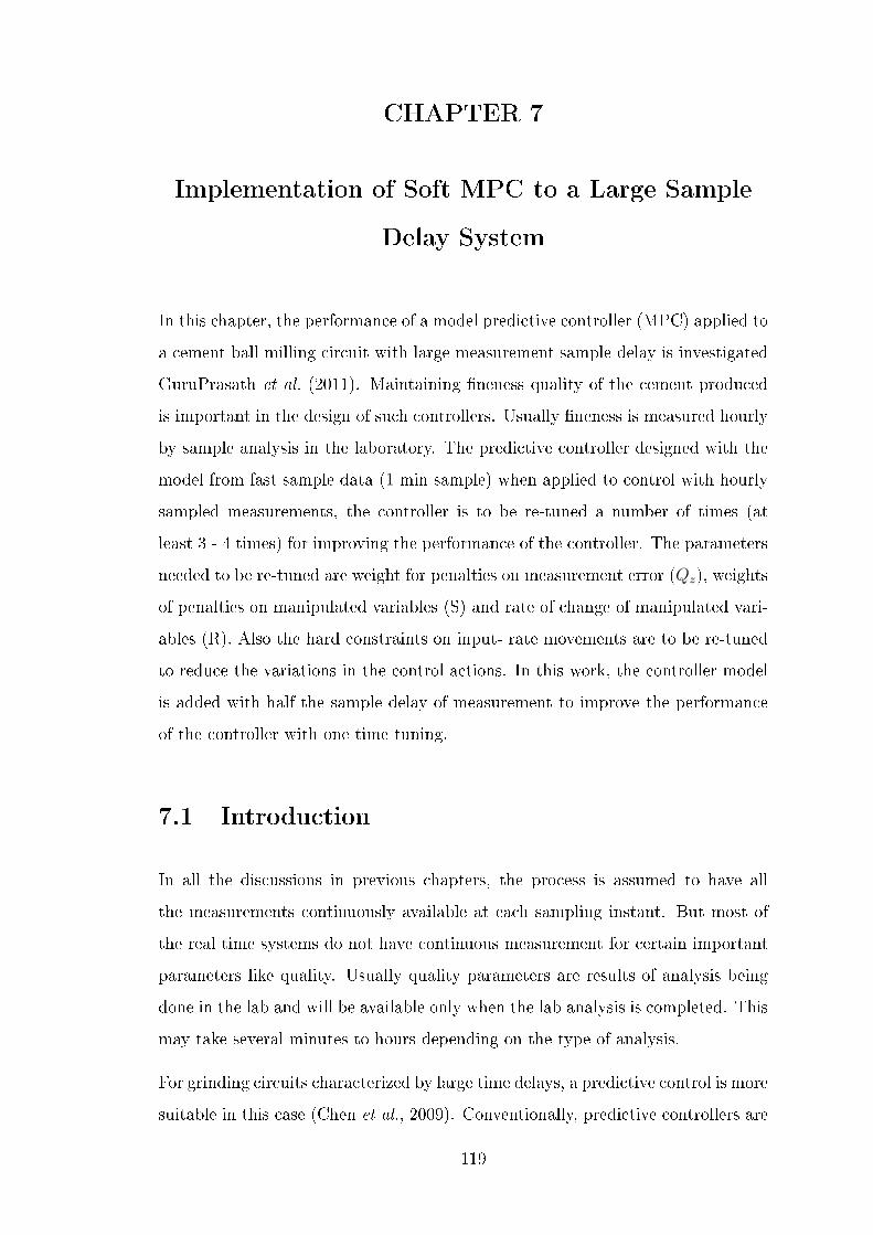
CHAPTER 7
Implementation of Soft MPC to a Large Sample
Delay System
In this chapter, the performance of a model predictive controller (MPC) applied to
a cement ball milling circuit with large measurement sample delay is investigated
GuruPrasath et al. (2011). Maintaining neness quality of the cement produced
is important in the design of such controllers. Usually neness is measured hourly
by sample analysis in the laboratory. The predictive controller designed with the
model from fast sample data (1 min sample) when applied to control with hourly
sampled measurements, the controller is to be re-tuned a number of times (at
least 3 - 4 times) for improving the performance of the controller. The parameters
needed to be re-tuned are weight for penalties on measurement error (Qz), weights
of penalties on manipulated variables (S) and rate of change of manipulated vari-
ables (R). Also the hard constraints on input- rate movements are to be re-tuned
to reduce the variations in the control actions. In this work, the controller model
is added with half the sample delay of measurement to improve the performance
of the controller with one time tuning.
7.1 Introduction
In all the discussions in previous chapters, the process is assumed to have all
the measurements continuously available at each sampling instant. But most of
the real time systems do not have continuous measurement for certain important
parameters like quality. Usually quality parameters are results of analysis being
done in the lab and will be available only when the lab analysis is completed. This
may take several minutes to hours depending on the type of analysis.
For grinding circuits characterized by large time delays, a predictive control is more
suitable in this case (Chen et al., 2009). Conventionally, predictive controllers are
119

more accepted in real time control of cement mill circuits because of their proven
control methodology and robustness. Usually, the models used in the controller are
obtained from continuous measurements obtained by step tests on the cement mill
system. In the real plant, the elevator load is a continuous measurement where as
the quality measurement Fineness or Blaine is collected every 1 hour using auto
sampler, analyzed and entered as o-line measurement. This may result in getting
a measurement every hour after the sample is analyzed and this will be available
for control. Thus, when conventional controller applied to such measurement the
controller parameters need to be re-tuned quite often to improve the controller
performance.
A nite impulse response (FIR) model based MPC is considered for controlling the
cement mill circuit. The cement mill control involves the control of mill loading
and neness. The main measure of neness is specic surface. Because cement
particles react with water at their surface, the specic surface area is directly re-
lated to the cement's initial reactivity. By adjusting the neness of grind, a range
of products can be produced from a single clinker. Tight control of neness is
necessary in order to obtain cement with the desired consistent day-to-day perfor-
mance. Thus neness control is one of the most important parameter in cement
mill control circuit. Fineness values can be obtained approximately once in an
hour as it is measured in lab by sample analysis. But the models on elevator load
representing the loading on the mill and neness for the controller are obtained at
each sampling instant from step response experiments conducted on the cement
mill simulation circuit. When such controllers are taken online to control hourly
sampled measurements the control performance becomes poor and the control pa-
rameters need to be re-tuned as discussed above. These kind of problems can
be solved as an multi-rate control problem. But here the problem is considered
as a sample measurement delay problem and a method is proposed to eectively
address the large sample delay measurements which signicantly improve the per-
formance of the controllers without much eort on tuning the system.
A method is proposed, in which the controller model is added with half the sample
delay of the measurement and the performance of the controller is analyzed.
120

Figure 7.1: Operator station of High Level Control for closed loop cement millFLSmidthA/S (2004).
7.2 System Implementation
The schematic diagram of ball mill control is shown in Figure 7.1.
The controllers are designed for handling dierent recipes where the operating
parameters/ targets will be changed depending on the type of recipe. The main
control loops considered are Feed rate and Fineness control. In addition for im-
proving the performance of cement mill operation and to achieve better stability
in the system, some of the control variables like dierential pressure across the
diaphragm, outlet temperature of the material and load on the separator fan are
to be controlled. These variables even though do not contribute in cement mill
performance signicantly, the uctuations in these variables cause the mill to be
unstable. Such control variables can be handled by simple SISO control/ PID
loops.
As discussed, the most important parameters that determine the performance of
the mill is the amount of material loading inside the mill and the quality of cement
being produced. Quality of nal product in the cement ball mill remains one of the
challenging and important parameter to be controlled. The quality is measured in
121

terms of neness of the cement by collecting samples from the nal product and
entered manually every hour in the supervisory system. A 2 × 2 MPC system is
considered based on the models as given in section 5.4. The controller actions can
be tuned from the tool available in the SCADA, called as Process Expert tool.
This is a visual basic programming environment interfaced with other tools like
Matlab, Excel etc., In this tool the tuning parameters can be directly entered from
the available ECS/SCADA and the values can be taken to the PLC for overwriting
the manual actions. Most important tuning parameters in the MPC are penalty
on the actuator movements to restrict the amount of control actions and weight
on the measurements to make the controlled variables to reach the desired targets.
The controller with model obtained from continuous sample data is made online in
the ECS/CEMulator system with Feed and Separator Speed controlling Elevator
Load and Fineness. Fineness of the cement controlled here is assumed to be hourly
sample collected from the nal product belt through an auto- sampler or manual
spot collection and the samples are analyzed and entered from the quality lab.
Thus the neness value is updated in the system with a delay of one hour.
The following tuning and weighting factors are used, while applying the MPC to
control the grinding circuit when the neness measured using an online analyzer:
Prediction horizon Np = 250, control horizon N = 50, The penalties on the errors
are
Qz =
0.5 0
0 0.015
, the penalties on the manipulated variables are
S =
100 0
0 1000
.When the above tuning parameters are used for controlling, the hourly neness
data the performance of the controller degrades, thus for improving the perfor-
mance of the MPC the control weights are needed to be re-tuned by trial and error
after a number of times (here the stable operating parameters are obtained after
4 trials) as
122

Qz =
0.1 0
0 0.001
, the weights on the manipulated variables
S =
100 0
0 10000
.
0 0.5 1 1.5 2 2.5 3 3.5 4 4.524
26
28
30
32
34
Ele
vato
r L
oad(
Kw
)
0 0.5 1 1.5 2 2.5 3 3.5 4 4.5
3000
3100
3200
3300
3400
Time(hrs)
Fine
ness
(cm
2/g)
0 0.5 1 1.5 2 2.5 3 3.5 4 4.5
70
80
90
Sepa
rato
r Sp
eed(
%)
0 0.5 1 1.5 2 2.5 3 3.5 4 4.5100
120
140
160
Time(hrs)
Feed
(t/h
)
Figure 7.2: Variations in MPC with nominal models when applied to measure-ments having large sample delays, Target(Red), Actual Value(Blue).
0 1 2 3 4 5 6 724
26
28
30
32
34
Ele
vato
r lo
ad(K
w)
0 1 2 3 4 5 6 7
3000
3100
3200
3300
3400
Time(hrs)
Fine
ness
(cm
2/g)
0 1 2 3 4 5 6 7
70
80
90
Sepa
rato
r Sp
eed(
%)
0 1 2 3 4 5 6 7100
120
140
160
Time(hrs)
Feed
(t/h
)
Figure 7.3: Variations in MPC with models including sample delay added to con-tinuous model and taken online for controlling the large sample delayparameters(Fineness), Target(Red), Actual Value(Blue).
These tuning values are obtained by trial and error method, depending on the
control actions of the controller. It can be seen that the penalty on Fineness is
very small, this is because the neness is a hourly sampled data and less reliable
when compared with elevator load. Also the penalty on separator speed moves is
set to a large value because varying the separator continuously causes wear in the
separator blades thus reducing the separation eciency in the long time. Thus the
control actions become less aggressive as the penalty on the actuator movement
123

(especially separator speed) is increased. This results in slower control actions on
both neness and elevator load making the controller sluggish. From Figure 7.2,
it is seen that the controlled variable Elevator load settles at approximately 3.5
hours and there is an steady state oset in case of Fineness measurement. The
actuator variations are also undesirable as it is quite oscillatory.
In order to avoid such a situation, the controller model for Fineness versus Feed and
separator speed are added with time delay which is considered to be approximately
half the sample delay of Fineness measurement. For example, with an hourly
sample measurement of neness we include a delay of 30 min in the neness model
of the controller as in Equation 7.1
G(s) =
0.62(45s+1)(8s+1)
e−5s 0.29(8s+1)(2s+1)(38s+1)
e−31.5s
(−15)(60s+1)
e−35s 5(14s+1)(s+1)
e−0.1s
(7.1)
When the predictive controller uses the model as in Equation 7.1, the performance
of the controller signicantly improve. The comparison of the controller with inclu-
sion of half the sample delay in the model with that of the conventional controller
is shown in Table 7.1. Also the proposed controller stabilizes the process much
faster when compared to the conventional predictive controller. The penalties on
the actuator and the control weights are kept the same that is used for nominal
model. Thus the tuning of the control weights is done only once in this case. From
Figure 7.3 it is seen that the Elevator load settles approximately in an hour and
the standard deviation of Fineness is close to zero. Thus it is observed that the
inclusion of half the sample delay in the controller model signicantly reduces the
tuning of system and also improves the stabilization of the process.
7.3 Conclusion
A method to use the MPC in an ecient way, for handling the large sample
delay cement mill systems is provided. When both the controllers are applied for
the control on cement mill using CEMulator with large delay measurements, the
124

Conventional Control(MPC) MPC with Sample Delay1. Model from CEMulator used forreal-time control
1. Model is added with approxi-mately half the sample delay
2. Controller need to be retuned forparameters like actuator movementweight(S), weight on measurementerror (Qz) etc., for each of the con-trolled variables and the parametersare to be re-tuned based on trial anderror method
2. Only the transfer function to bechanged and no further tuning re-quired. This alters the bias term inthe estimator used as controller feed-back
3. Provide sluggish operation or actevery hour
3. Changes in model aect the FIRco-ecients and prediction calcula-tions GuruPrasath and Jorgensen(2009), by altering the hessian ma-trix values in the optimization solu-tion.
Table 7.1: Comparison of Conventional control and Controller with sample Delay.
controller with continuous sample model needs to be re-tuned a number of times (
3−4 times in this case) in order to improve the controller performance on dierent
conditions. The settling time is approximately 3.5 hours in case of Elevator load
and results in steady state oset of Fineness. By applying the proposed method
in which half the sample delay is included with the existing delay in the model, a
signicant performance improvement is obtained in terms of stability and settling
time of the process(a settling time of around 1 hour for Elevator load and almost
zero standard deviation for Fineness) with little tuning (the tuning is done only
once in this case).
125

CHAPTER 8
Summary and Conclusions
This work focusses on design of Finite Impulse Response based MPC for uncer-
tain systems. Further, a simple moving horizon estimator is designed to improve
the performance of the controller. Finally a soft constraint based MPC is devel-
oped and experimentally implemented on a cement mill circuit. Also an improved
method of MPC design for large sample delay systems is proposed and imple-
mented in a simulator. The results obtained in each section are summarized as
below
8.1 An evaluation of existing MPC tools
Based on nite impulse response predictions, a regularized l2 predictive controller
with input and input-rate constraints is analyzed. An estimator based on a simple
constant output disturbance lter is developed for the feed back. The FIR based
regulator problem is solved by convex quadratic program (QP) by converting the
objective function into a standard form. The QP is solved using an algorithm
based on interior point method. Illustrative examples are given to understand the
eect of uncertainties in the model based controllers. The results are veried by
testing the controller with scalar SOPDT with a zero transfer function model.
A moving horizon estimator based on Finite impulse response models is developed.
The estimator is used to estimate the unknown disturbance by solving the objective
function. The estimated disturbance is then used as a feedback to the controller.
The objective function solved for estimation is convex QP similar to the regulator
problem. To improve the performance of the MPC, the estimator is then made
closed loop with the regulator by replacing the simple integrator developed in
the previous section. By using a SOPDT with a zero transfer function model
126

the performance of the estimator with measurement noise is provided. Also the
closed loop performance of a model predictive controller consisting of a predictive
regulator and estimator with SISO system is investigated.
A ℓ2 regularized predictive controller with soft output constraints along with hard
input and input-rate constraints is developed and the ecient application of this
controller to uncertain stochastic systems is demonstrated. The predictive con-
troller is equipped with soft output constraints that are used in a novel way to
have robustness against model plant mismatch. The QP is solved similar to the
standard form. The estimator used here is the simple output disturbance lter.
The control algorithm designed is then solved using interior point algorithm.
8.2 Comparison of soft MPC with conventional
MPC
By simulation, rst with SISO system and then with 2X2 MIMO system, the
performance of the new robust constrained predictive controller to a conventional
predictive controller is investigated. Finite impulse response coecients for the
models are obtained with step tests conducted on a simulated cement mill circuit.
Improved performances are obtained with the soft MPC developed than that of
the conventional MPC when the controllers are taken in closed loop simulation.
8.3 Application of Soft MPC in cement mill circuit
The proposed model predictive controller which includes the soft output con-
straints is made online with the cement mill circuit using a simulator. The con-
troller is mainly used to control elevator power and neness of the cement mill as
they contribute to production and quality. Step response tests are conducted in
the cement mill circuit and a SOPDT with a zero transfer function model is de-
veloped. Grindability is taken as the disturbance parameter. Uncertainties in the
simulator are generated by changing the grindability of the input feed material.
127

The controller performance is compared in the simulator by running the controllers
online for 16 hours each. The conditions for the simulations are kept similar both
in conventional MPC and soft MPC to have a perfect comparison. This is done by
creating simulation tutorials where the disturbances are given exactly at the same
time for both the controllers after taken online. The performance of the soft MPC
is better than the conventional MPC with uncertainties present in the system.
Real time implementation
The proposed controller is applied to a real time cement plant. The controller is
compared with Fuzzy logic controller available in plant. The controller is interfaced
with the real time ECS/SCADA so that the set points generated by the controller
are directly entered into the eld PLC. The controllers are designed for handling
dierent recipes where the operating parameters will be changed depending on
the type of recipe. The main control loops considered are Feed and Fineness
control. The simple loops in the circuit are controlled with the PIDs available in
the PLC. This is to improve the stability of the circuit and have same conditions
for comparing both the controllers. Quantitative performance improvements of
soft MPC over the fuzzy logic controller are obtained.
8.4 Implementation of Soft MPC to a Large Sam-
ple Delay System
A method to design the MPC more robust in handling the large sample delay ce-
ment mill systems is provided. By simulation for MIMO systems the performance
of soft MPC and conventional MPC with models obtained from continuous sam-
pling of data are compared. The controllers are tested in cement mill simulator
circuit as in the previous section. Elevator power and Fineness are the controlled
variables. Feed rate and separator speed are the manipulated variables. The pre-
dictive controller designed with the model from fast sample data (1 min sample)
when applied to control with hourly sampled measurements, the controller is to be
re-tuned. The parameters needed to be re-tuned are weight for penalties on mea-
128

surement error (Qz), weights of penalties on manipulated variables (S) and rate
of change of manipulated variables (R). Also the hard constraints on input- rate
movements are to be re-tuned to reduce the variations in the controller. In this
work, the controller model is added with half the sample delay of measurement to
improve the performance of the controller with one time tuning.
8.5 Conclusions
The following conclusions are drawn based on the above investigations:
1. It is veried by simulations that the closed-loop MPC performance degrada-
tion due to plant-model mismatch is tightly related to the uncertainty of impulse
response coecients. The closed loop performance of the controller is good when
the uncertainty in each of the parameters (separately in gain, zero and time delay)
are smaller(upto 40 % incase of time delay, 50 % in gain and twice incase zero)
with that of the nominal model. The controller performance reaches sustained
oscillations when the uncertainty in each of these parameters exceeds the above
these values. Also presence of noise in the system further degrades the closed loop
performance of the controller. The simulations in the present work provide as the
potential as well as expected limits on the performance improvement that can be
achieved by robust MPC, i.e. an upper limit on the potential performance is the
performance of the nominal model.
2. The performance of soft MPC is compared with conventional MPC through
simulations. From the simulations it is observed that with the uncertainties of the
model parameters, the conventional MPC provides sustained oscillations when the
model mismatch becomes twice(in-terms of gain, time delay and time constants at
each instant) that of the nominal model. In case of soft MPC the oscillations are
suppressed completely and the system settles before 75% of the control horizon.
Thus the soft MPC provides much better performance improvement in the face of
plant-model mismatch than the conventional MPC.
3. The performance of the proposed controllers are evaluated by simulation using
129

the transfer functions on MIMO models. It is observed that the soft MPC varies
the actuator very little when the controlled variables are within the soft limits. In
case of conventional MPC the controller makes aggressive moves on the actuator
for settling the output variables which is an undesirable action especially in real
time plants. The variations in the output variables are similar in both the con-
trollers, but soft MPC achieves the variation with smaller actuator moves. The
standard deviation of feed rate in conventional MPC is 4.4258 and separator speed
is 2.4149.The standard deviation of feed rate in soft MPC is 3.269 and separator
speed is 0.0878. Also the initial variation in feed and separator speed are high in
case of conventional MPC when compared with soft MPC. Thus soft MPC pro-
vides lesser actuator variations which is mostly preferred in plant when compared
with the conventional MPC.
4. The proposed controller with soft output constraints for handling the uncer-
tainties of the cement mill circuit is implemented in a real plant. The predictive
controller is compared with the high level Fuzzy Logic controller existing in the
plant. It is observed that when both the controllers are made online with similar
process conditions and in the same recipe, the standard deviation in the quality
parameter (i.e Fineness of the product) is reduced by around 23% with soft MPC
when compared with that of FLC in the plant. Also the stability of the system
is improved with much simpler and smaller actuator variations in soft MPC when
compared with the FLC.
5. The proposed controller is tested with cement mill simulator with large sample
delay. It is observed that incase of plant-model mismatch, the soft MPC sup-
presses the sustained oscillations by smaller actuator moves when compared to
the conventional MPC. The same MPC when applied for cement mill control with
large sample delay measurements the regularization weights (R and S)need to be
re-tuned a number of times (at least 3 to 4 times in this case) to improve the
performance of the controller. In this case the regularization weights are increased
for making the controller actions sluggish. This results in longer settling time (ap-
proximately 3.5 hours in case of Elevator load and steady state oset of Fineness)
of the controlled variables. By simulations, it is demonstrated that the proposed
130

method gives a signicant improvement in the stability of the process, (a settling
time of around 1 hour for Elevator load and almost zero standard deviation for
Fineness).
Future Scope
The estimation in the MPC proposed can be further improved by using standard
time series models like ARMA, ARMAX etc., which can be obtained using stan-
dard identication techniques and the controller performance can be investigated
with the inclusion of such estimators.
In real time comparison of the soft MPC with other controllers, the performance
of both the controllers can be done by keeping certain operating conditions like
comparison with respect to same settling time of output etc., This will provide a
platform in which the best tuned controllers are compared for a given condition.
The research can be further extended in developing a robust controller based on
Second Order Cone Programming (SOCP) technique which can inherently handle
uncertainties and disturbances in the system.
131

APPENDIX A
Quadratic Program Formulation
A.1 Quadratic program for FIR based MPC
Dene the vectors Z, R, and U as
Z =
z1
z2...
zN
R =
r1
r2...
rN
U =
u0
u1...
uN−1
(A.1)
Then the predictions by the impulse response model in Equation 3.6b may be
expressed as
Z = c+ ΓU (A.2)
For the case N = 6 and n = 3, Γ is assembled as
Γ =
H1 0 0 0 0 0
H2 H1 0 0 0 0
H3 H2 H1 0 0 0
0 H3 H2 H1 0 0
0 0 H3 H2 H1 0
0 0 0 H3 H2 H1
(A.3)
and c is
c =
c1
c2
c3
c4
c5
c6
=
b1 + (H2u−1 +H3u−2)
b2 + (H3u−1)
b3
b4
b5
b6
(A.4)
132

Similarly, for the case N = 6, dene the matrices Λ and I0 by
Λ =
I 0 0 0 0 0
−I I 0 0 0 0
0 −I I 0 0 0
0 0 −I I 0 0
0 0 0 −I I 0
0 0 0 0 −I I
I0 =
I
0
0
0
0
0
(A.5)
and
Qz =
Qz
Qz
. . .
Qz
S =
S
S. . .
S
(A.6)
The objective function in Equation 3.6a may be expressed as
ϕ =1
2
N−1∑k=0
∥zk+1 − rk+1∥2Qz+ ∥∆uk∥2S
=1
2∥Z −R∥2Qz
+1
2∥ΛU − I0u−1∥2S
=1
2∥c+ ΓU −R∥2Qz
+1
2∥ΛU − I0u−1∥2S
=1
2U ′ (Γ′QzΓ + Λ′SΛ)U
+ (Γ′Qz(c−R)− Λ′SI0u−1)′U
+
(1
2∥c−R∥2Qz
+1
2∥I0u−1∥2S
)=
1
2U ′HU + g′U + ρ
(A.7)
in which
H = Γ′QzΓ + Λ′SΛ (A.8a)
g = Γ′Qz(c−R)− Λ′SI0u−1 (A.8b)
ρ =1
2∥c−R∥2Qz
+1
2∥u−1∥2S (A.8c)
133

Consequently, the FIR based MPC regulator problem in Equation 3.6 can be
solved by nding the solution of the following convex quadratic program
minU
ψ =1
2U ′HU + g′U (A.9a)
s.t. Umin ≤ U ≤ Umax (A.9b)
bl ≤ ΛU ≤ bu (A.9c)
in which
Umin =
umin
umin
...
umin
Umax =
umax
umax
...
umax
(A.10)
and
bl =
∆umin + u−1
∆umin
...
∆umin
bu =
∆umax + u−1
∆umax
...
∆umax
(A.11)
In a model predictive controller only the rst vector, u∗0, of U∗ =
[(u∗0)
′ (u∗1)′ . . . (u∗N−1)
′]′,
is implemented on the process. At the next sample time the open-loop optimiza-
tion is repeated with new information due to a new measurement.
A.2 Quadratic Program formulation for Estimator
Estimation problem can be formulated by considering a nite impulse response
(FIR) model
zk = bk +n∑
i=0
Hiuk−i +n∑
i=1
Hiddk−i (A.12)
in which Hini=0 are the impulse response coecients. Here the moving horizon
estimator are based on the FIR model.
Using the transfer function model, the estimation problem can be formulated as
134

minz,d
ϕ =1
2
Ne∑k=0
∥zk − yk∥2Qz+ ∥∆dk∥2S + ∥dk∥2R (A.13a)
s.t. zk = bk +n∑
i=0
Hd,idk−i (A.13b)
dmin ≤ dk ≤ dmax k = 0, . . . , Ne (A.13c)
∆dmin ≤ ∆dk ≤ ∆dmax k = 0, . . . , Ne (A.13d)
where bk = bk +n∑
i=1
Hu,iuk−i k = 1, . . . , Ne (A.13e)
It is assumed that di−ni=−1 are disturbance values xed at their previous estimates
such that the real decision variables in Equation A.13e are dkNe
k=0. The decision
variables are normally split into a slow varying component (level), dk and a rapid
varying component (process noise), wk, the constraints will have the following
interpretation,
dk =
dkwk
, dmin =
dmin
wmin
, dmax =
dmax
wmax
∆dmin =
∆dmin
∆wmin
and ∆dmax =
∆dmax
∆wmax
Typically ∆wmin = −∞, ∆wmax =∞ and ∆wk is not penalized in the objec-
tive function in order not to restrict the movements of rapid varying component
of the unknown disturbance. However the size of wk may be constrained and pe-
nalized in the objective function. Oppositely only the rate of movement of the
slowly varying component is penalized. Consequently the weight matrices S and
R have the structure
S =
Sd 0
0 0
, R =
0 0
0 Rw
(A.14)
The typical case with Hd,i =[Hd,i Hw,i
]and Hd,i = Hw,i corresponds to an
unknown disturbance of the form dk = dk + wk.
135

Here an approach to formulate a dense quadratic program in standard form equiva-
lent with Equation (A.13a) is provided. This is done by elimination of the outputs,
zkNe
k=0 from the optimization problem (Equation A.13a).
Dene the vectors Z, Y , and D as
Z =
z1
z2...
zN
Y =
y1
y2...
yN
D =
d0
d1...
dN−1
(A.15)
Then the predictions by the impulse response model (Equation A.13b) may be
expressed as
Z = c+ ΓD (A.16)
For the case N = 6 and n = 3, Γ is assembled as
Γ =
Hd,0 0 0 0 0 0 0
Hd,1 Hd,0 0 0 0 0 0
Hd,2 Hd,1 Hd,0 0 0 0 0
Hd,3 Hd,2 Hd,1 Hd,0 0 0 0
0 Hd,3 Hd,2 Hd,1 Hd,0 0 0
0 0 Hd,3 Hd,2 Hd,1 Hd,0 0
0 0 0 Hd,3 Hd,2 Hd,1 Hd,0
(A.17)
and c is
c =
c0
c1
c2
c3
c4
c5
c6
=
b0 +∑3
i=1Hu,iu0−i +∑3
i=1Hd,id0−i
b1 +∑3
i=1Hu,iu1−i +∑3
i=2Hd,id1−i
b2 +∑3
i=1Hu,iu2−i +∑3
i=3Hd,id2−i
b3 +∑3
i=1Hu,iu3−i
b4 +∑3
i=1Hu,iu4−i
b5 +∑3
i=1Hu,iu5−i
b5 +∑3
i=1Hu,iu6−i
(A.18)
136
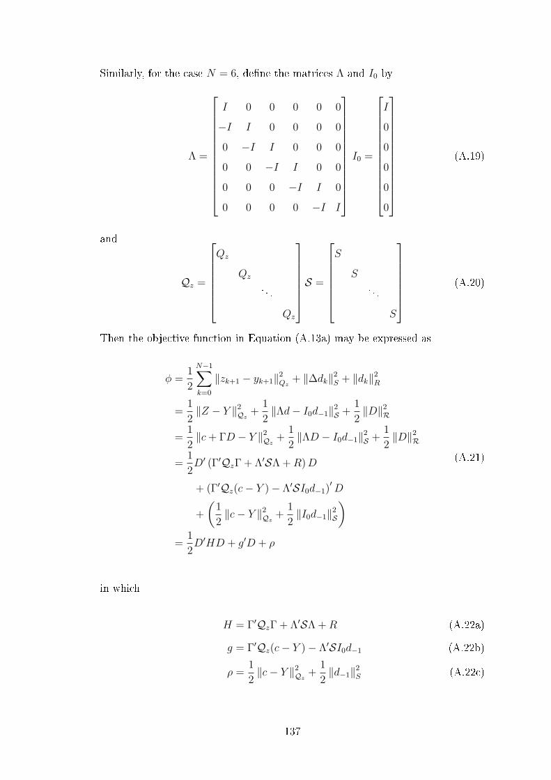
Similarly, for the case N = 6, dene the matrices Λ and I0 by
Λ =
I 0 0 0 0 0
−I I 0 0 0 0
0 −I I 0 0 0
0 0 −I I 0 0
0 0 0 −I I 0
0 0 0 0 −I I
I0 =
I
0
0
0
0
0
(A.19)
and
Qz =
Qz
Qz
. . .
Qz
S =
S
S. . .
S
(A.20)
Then the objective function in Equation (A.13a) may be expressed as
ϕ =1
2
N−1∑k=0
∥zk+1 − yk+1∥2Qz+ ∥∆dk∥2S + ∥dk∥2R
=1
2∥Z − Y ∥2Qz
+1
2∥Λd− I0d−1∥2S +
1
2∥D∥2R
=1
2∥c+ ΓD − Y ∥2Qz
+1
2∥ΛD − I0d−1∥2S +
1
2∥D∥2R
=1
2D′ (Γ′QzΓ + Λ′SΛ +R)D
+ (Γ′Qz(c− Y )− Λ′SI0d−1)′D
+
(1
2∥c− Y ∥2Qz
+1
2∥I0d−1∥2S
)=
1
2D′HD + g′D + ρ
(A.21)
in which
H = Γ′QzΓ + Λ′SΛ +R (A.22a)
g = Γ′Qz(c− Y )− Λ′SI0d−1 (A.22b)
ρ =1
2∥c− Y ∥2Qz
+1
2∥d−1∥2S (A.22c)
137

Consequently, the FIR based Estimator problem can be solved by the solution of
the following convex quadratic program
minD
ψ =1
2D′HD + g′D (A.23a)
s.t. Dmin ≤ D ≤ Dmax (A.23b)
bl ≤ ΛD ≤ bu (A.23c)
in which
Dmin =
dmin
dmin
...
dmin
Dmax =
dmax
dmax
...
dmax
(A.24)
and
bl =
∆dmin + d−1
∆dmin
...
∆dmin
bu =
∆dmax + d−1
∆dmax
...
∆dmax
(A.25)
A.3 Quadratic Program formulation for Soft MPC
Dene the vectors Z, R, and U as
Z =
z1
z2...
zN
R =
r1
r2...
rN
U =
u0
u1...
uN−1
(A.26)
Then the predictions by the impulse response model in Equation (3.22) may be
expressed as
Z = c+ ΓU (A.27)
138

For the case N = 6 and n = 3, Γ is assembled as
Γ =
H1 0 0 0 0 0
H2 H1 0 0 0 0
H3 H2 H1 0 0 0
0 H3 H2 H1 0 0
0 0 H3 H2 H1 0
0 0 0 H3 H2 H1
(A.28)
and c is
c =
c1
c2
c3
c4
c5
c6
=
b1 + (H2u−1 +H3u−2)
b2 + (H3u−1)
b3
b4
b5
b6
(A.29)
Similarly, for the case N = 6, dene the matrices Λ and I0 by
Λ =
I 0 0 0 0 0
−I I 0 0 0 0
0 −I I 0 0 0
0 0 −I I 0 0
0 0 0 −I I 0
0 0 0 0 −I I
I0 =
I
0
0
0
0
0
(A.30)
Dene sη =[sη1
′ sη1′ . . . sηN
′]′and
Qz =
Qz
Qz
. . .
Qz
S⟩ =Si
Si
. . .
Si
(A.31)
139

with i = u, η. Then the objective function in Equation (3.22) may be expressed
as
ϕ =1
2
N−1∑k=0
∥zk+1 − rk+1∥2Qz+ ∥∆uk∥2S +
1
2∥ηk+1∥2Sη
+ s′ηk+1ηk+1
=1
2∥Z −R∥2Qz
+1
2∥ΛU − I0u−1∥2S +
1
2∥η∥2Sη
+ s′ηη
=1
2∥c+ ΓU −R∥2Qz
+1
2∥ΛU − I0u−1∥2S
+1
2∥η∥2Sη
+ s′ηη
=1
2U ′ (Γ′QzΓ + Λ′SΛ)U
+ (Γ′Qz(c−R)− Λ′SI0u−1)′U
+
(1
2∥c−R∥2Qz
+1
2∥I0u−1∥2S
)+
1
2η′Sηη + s′ηη
=1
2U ′HU + g′U + ρ+
1
2η′Sηη + s′ηη
=1
2x′Hx+ g′x+ ρ
(A.32)
140

in which
H = Γ′QzΓ + Λ′SΛ (A.33a)
g = Γ′Qz(c−R)− Λ′SI0u−1 (A.33b)
ρ =1
2∥c−R∥2Qz
+1
2∥u−1∥2S (A.33c)
x =
Uη
(A.33d)
H =
H 0
0 Sη
(A.33e)
g =
gsη
(A.33f)
Consequently, we may solve the FIR based MPC regulator problem in Equation
(3.22) by solution of the following convex quadratic program
minx
ψ =1
2x′Hx+ g′x (A.34a)
s.t. xmin ≤ x ≤ xmax (A.34b)
bl ≤ Ax ≤ bu (A.34c)
in which
A =
Λ 0
Γ −I
Γ I
(A.35a)
xmin =
Umin
0
xmax =
Umax
∞
(A.35b)
where
Umin =
umin
umin
...
umin
Umax =
umax
umax
...
umax
(A.36)
141
and
bl =
∆Umin
−∞
Zmin − c
bu =
∆Umax
Zmax − c
∞
(A.37)
In a model predictive controller only the rst vector,
u∗0, of U∗ =
[(u∗0)
′ (u∗1)′ . . . (u∗N−1)
′]′, is implemented on the process. At the
next sample time the open-loop optimization is repeated with new information
due to a new measurement.
142
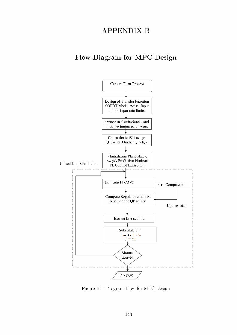
APPENDIX B
Flow Diagram for MPC Design
Figure B.1: Program Flow for MPC Design
143

APPENDIX C
General Form of Quadratic Program
C.1 Quadratic Program Formulation
Dene the vectors Z, R, and U as
Z =
z1
z2...
zN
R =
r1
r2...
rN
U =
u0
u1...
uN−1
(C.1)
Then the predictions by the impulse response model in Equation (3.22) may be
expressed as
Z = c+ ΓU (C.2)
In the general form Γ is assembled as
Γ =
H1 0 0 0 0 0
H2 H1 0 0 0 0... H2 H1 0 0 0
H(N − n) . . . H2 H1 0 0
0 H(N − n) . . . H2 H1 0
0 0 H(N − n) . . . H2 H1
(C.3)
144

and c is
c =
c1
c2
c3
c4
c5...
cN
=
b1 + (H2u−1 +H3u−2)
b2 + (H3u−1)
b3
b4...
b5
bN
(C.4)
Similarly, dene the matrices Λ and I0 by
Λ =
I 0 0 0 0 0
−I I 0 0 0 0
0 −I I 0 0 0
0 0 −I I 0 0
0 0 0 −I I 0
0 0 0 0 −I I
N×N
I0 =
I
0
0
0
0
0
N×1
(C.5)
Dene sη =[sη1
′ sη1′ . . . sηN
′]′and
Qz =
Qz
Qz
. . .
Qz
S⟩ =Si
Si
. . .
Si
(C.6)
with i = u, η. Then the objective function in Equation (3.22) may be derived
as in Appendix A.3, then converted to the general convex quadratic program
minx
ψ =1
2x′Hx+ g′x (C.7a)
s.t. xmin ≤ x ≤ xmax (C.7b)
bl ≤ Ax ≤ bu (C.7c)
145

in which
A =
Λ 0
Γ −I
Γ I
(C.8a)
xmin =
Umin
0
xmax =
Umax
∞
(C.8b)
where
Umin =
umin
umin
...
umin
Umax =
umax
umax
...
umax
(C.9)
and
bl =
∆Umin
−∞
Zmin − c
bu =
∆Umax
Zmax − c
∞
(C.10)
In a model predictive controller only the rst vector,
u∗0, of U∗ =
[(u∗0)
′ (u∗1)′ . . . (u∗N−1)
′]′, is implemented on the process. At the
next sample time the open-loop optimization is repeated with new information
due to a new measurement.
146
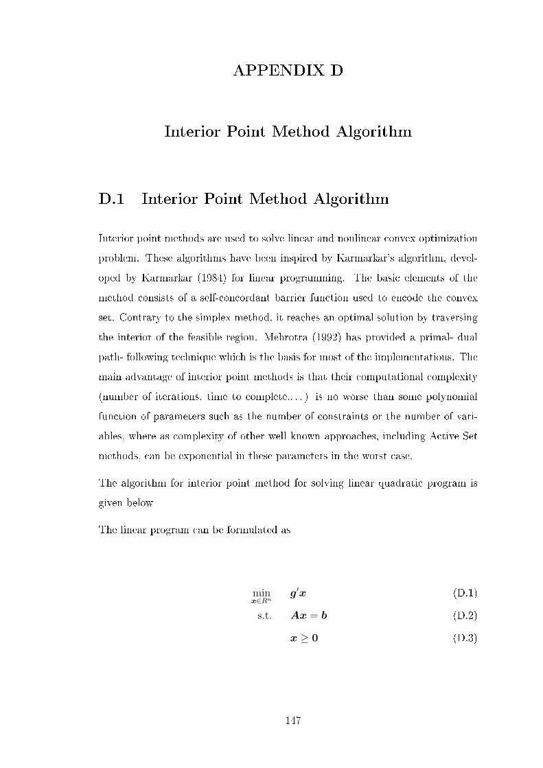
APPENDIX D
Interior Point Method Algorithm
D.1 Interior Point Method Algorithm
Interior point methods are used to solve linear and nonlinear convex optimization
problem. These algorithms have been inspired by Karmarkar's algorithm, devel-
oped by Karmarkar (1984) for linear programming. The basic elements of the
method consists of a self-concordant barrier function used to encode the convex
set. Contrary to the simplex method, it reaches an optimal solution by traversing
the interior of the feasible region. Mehrotra (1992) has provided a primal- dual
path- following technique which is the basis for most of the implementations. The
main advantage of interior point methods is that their computational complexity
(number of iterations, time to complete,. . . ) is no worse than some polynomial
function of parameters such as the number of constraints or the number of vari-
ables, where as complexity of other well known approaches, including Active Set
methods, can be exponential in these parameters in the worst case.
The algorithm for interior point method for solving linear quadratic program is
given below
The linear program can be formulated as
minx∈Rn
g′x (D.1)
s.t. Ax = b (D.2)
x ≥ 0 (D.3)
147

The Lagrangian function can be given as
L(x,µ,λ) = g′x− µ′(Ax− b)− λ′x (D.4)
The optimality conditions are
∇xL(x,µ,λ) = g −A′µ− λ = 0 (D.5)
Ax = b (D.6)
x ≥ 0 (D.7)
λ ≥ 0 (D.8)
xiλi = 0, i = 1, 2, . . . ,mC (D.9)
These can be expressed as
rL = ∇xL = g −A′µ− λ = 0 (D.10a)
rA = Ax− b = 0 (D.10b)
XΛe = 0 (D.10c)
x ≥ 0 (D.10d)
λ ≥ 0 (D.10e)
Thus the optimality conditions in matrix form is
F (x,µ,λ) =
g −A′µ− λ
Ax− b
XΛe
=
0
0
0
= 0 (D.11a)
These conditions can thus be solved using Newton like method after forming the
matrix as shown below
148

F(x, µ, λ) =
0 −A′ −I
A 0 0
Λ 0 X
∆x
∆µ
∆λ
= −
rL
rA
rC
,x ≥ 0, λ ≥ 0.
where: x
µ
λ
←
x
µ
λ
+ α
∆x
∆µ
∆λ
For solving the above matrix rst we have to dene the ane direction (∆xaff ,∆µaff ,∆λaff)T
by solving0 −A′ −I
A 0 0
Λ 0 X
∆xaff
∆µaff
∆λaff
= −
g −A′µ− λ
Ax− b
XΛe
= −
rL
rA
rC
(D.12)
Then we have to nd the largest ane step
αaff and βaff such that
x+ αaff∆xaff ≥ 0, λ+ βaff∆λaff ≥ 0 (D.13)
Compute the aned duality gap
saff = (x+ αaff∆xaff)′(λ+ βaff∆λaff)/n (D.14)
where n is the dimension of x.
Thus for center step we have to introduce a duality measure :
s =x′λ
n,
and the centering parameter
149

σ = (saff/s)3,
We solve the nal equation after improving it by a corrector step and computing
the centering parameter as
0 −A′ −I
A 0 0
Λ 0 X
∆x
∆µ
∆λ
= −
rL
rA
rC +∆Xaff∆Λaffe− σse
,
Further we compute the largest step length α and β such that
x+ α∆x ≥ 0, λ+ β∆λ ≥ 0 (D.15)
and update x, µ and λ by x
µ
λ
←
x+ ηα∆x
µ+ ηβ∆µ
λ+ ηβ∆λ
(D.16)
Thus by improving corrector step and computing the centering parameter, the
total step for solving next iteration is obtained.
The algorithm is specied here as below:
150

Predictor-Corrector Algorithm for QP
Compute (x0, µ0, λ0)
for k = 0, 1, 2, . . .
Set (x, µ, λ) = (xk, µk, λk) and solve (D.12)
for (∆xaff ,∆µaff ,∆λaff);
Calculate αaffandβaff as in (D.13);
Calculate saff = (x+ αaff∆xaff)T (λ+ βaff∆λaff)/n;
Set centering paramenter to σ = (saff/s)3;
Solve (D.1) for (∆x,∆µ,∆λ);
Calculate αaffandβaff as in (D.15);
Set (xk+1) = (xk) + α(∆x);
Set (µk+1, λk+1) = (µk, λk) + β(∆µ,∆λ);
end
151

APPENDIX E
Matlab Program for Soft MPC design
E.1 Initialization of MPC
%echo on
% Program f o r gene ra t ing the Simulat ion response f o r the
% So f t MPC with F in i t e Impulse Response Methods f o r
%second order Trans fe r Function with de lay time
%
% System De f i n i t i o n :
%
%Trans fe r Function Parameters
%
% K− Gain o f the system
% T1 ,T2− Time cons tant s
% beta − zero o f the system
% Td − Time delay o f the system
%
% Ts− Sampling Time
% Nsim − Simulat ion hor i zon
%
% Normal_MPC − Function f o r computing the con t r o l sequence
% us ing MPC without i n c l ud ing s o f t c on s t r a i n t l im i t s
% Soft_MPC − Function f o r MPC with s o f t Const ra in t s
%
% U − c on t r o l input to the system
% D − Disturbance in the system
% Y − Output o f the system inc l ud ing s t o c h a s t i c n o i s e s
152

% v − Measurement Noise
% w − Process Noise
% System De f i n i t i o n
c l o s e a l l
c l e a r a l l
c l c
% Parameters
K = [ 0 . 6 2 0.29;−15 5 ]
T1 = [45 2 ;60 14 ]
T2 = [8 38 ;0 1 ]
Td = [5 3 1 . 5 ; 5 3 0 . 1 ]
beta = [0 8 ;0 0 ]
t o l=1e−12;
%%%%
% K = [ 1 . 0 0 ;0 1 ]
% T1 = [5 0 ;0 5 ]
% T2 = [5 0 ;0 5 ]
% Td = [5 0 ;0 5 ]
% beta = [2 0 ;0 2 ]
%%%%
[ nz , nu]= s i z e (K)
dTs = 1 . 0 ;
n = 50 ;
Fs=18;
%% Design and Simulat ion o f MPC Parameters
Nsim = 500 ;
N = 2∗n ;
% Noise sequence
153

Qv=[0.00 0 ; 0 0 . 0 0 ] ;
Qw=[0.00 0 ;0 0 . 0 0 ] ;
%% Input Limits
umin = [−15;−30] ;
umax = [ 1 5 ; 3 0 ] ;
dumin = [ −1 .5 ; −0 .3 ] ;
dumax = [ 1 . 5 ; 0 . 3 ] ;
%%%%%%%%%%%%%%%%%%%%%%%%%%%%%%%%%%%%%%%%%%%%%%%%%%%%%%%
% Normal MPC Parameters
Qz = [8 0 ;0 1 . 0 ]
S = [ 1 . 0 e−8 0 ;0 1 .0 e−1]
%%%%%%%%%%%%%%%%%%%%%%%%%%%%%%%%%%%%%%%%%%%%%%%%%%%%%%%
% Sof t MPC Parameters
Qzs = [ 1 . 8 0 ; 0 0 .0000000002 ] ;
Ss = [8000 0 ;0 40000 ] ;
Sn =[9000 0 ;0 250 ] ; % Quadratic weight on So f t Limits
s n l i n = [ 0 ; 0 ] ; % Linear Weight on So f t Limits
%% System Model
[Uk, Sk ,Vk]= svd (K)
Skmod= [1∗ Sk ( 1 , : ) ; 1 . 0 ∗ Sk ( 2 , : ) ]
Knew=Uk∗Skmod∗Vk'
[ Ut , St , Vt]= svd (T1)
154

Stmod= [ 1 . 0 ∗ St ( 1 , : ) ; 1 . 0 ∗ St ( 2 , : ) ]
T1new=Ut∗Stmod∗Vt '
[Ud, Sd ,Vd]= svd (Td)
Sdmod= [1∗Sd ( 1 , : ) ; 1 . 0 ∗ Sd ( 2 , : ) ]
Tdnew=Ud∗Sdmod∗Vd'
%%
Knew=K
K1 = Knew%+[ 0 .4 0 .3 ;−8 4 ]
T11 = T1%+[ −15 −2 ; 0 0 ]
T21 = T2
Td1 = Td +[0 0 ; 0 0 ] %[ 5 −0.5 ; 6 1]%Tdnew
beta1 = beta%+[−0 ; 0 ]
%%
[A,B,C,D,H1]=MIMOSSModel( nz , nu ,N, Nsim ,K1, T11 , T21 , beta1 ,
Td1 , dTs , t o l ) ;
Bd=B;
Nx = s i z e (A, 1 ) ;
Nu = s i z e (B, 2 ) ;
Ny = s i z e (C, 1 ) ;
Nd= s i z e (Bd , 2 ) ;
%% MPC d e f i n i t i o n
% Parameters
Khat = K∗1 ;
T1hat = T1∗1 ;
T2hat = T2∗1 ;
Tdhat = Td∗1 ;
155

betahat = beta ∗1 ;
% Extract Impulse Response C o e f f i c i e n t s (SISO) f o r system
[ Ahat , Bhat , Chat , Dhat ,Himp]=MIMOSSModel( nz , nu ,N, Nsim , Khat ,
T1hat , T2hat , betahat , Tdhat , dTs , t o l ) ;
%% Noise and d i s turbance Generation
R = ones (Ny, Nsim+1)∗0;
[ v ,w] =MPC_noise(Qv,Qw,Nd,Ny, Nsim ) ;
D= 0∗ ones (Nd, Nsim ) ;
D( : , 2 1 : end ) = 3∗ ones ( 2 , 480 )∗1 ;
Dw = D +w;
x0 = ze ro s (Nx, 1 ) + 0∗ ones (Nx , 1 ) ;
%%% Sof t Limits
zmin = [0 −0 .8 ;0 −50 .0 ] ;
zmax = [0+0 . 8 ; 0+50 . 0 ] ;
%% Sof t MPC
[Y2 ,U2 ,R,FIRMPC2]=Soft_MPC_MIMO(Himp ,A,B,Bd ,C, Qzs , Ss ,
Sn , sn l i n ,R,Dw, v , x0 , umin , umax ,
dumin , dumax , zmin , zmax ,N,Nx,Nu,Ny, Nsim ) ;
%% Plot Resu l t s
f i g u r e (1 )
subplot (211)
s e t ( gca , ' FontName ' , ' Times ' , ' FontSize ' , Fs ) ;
p l o t ( 0 : Nsim ,Y2 ( 1 , : ) , ' r ' , ' l inewidth ' , 2 )
156
hold on
s t a i r s ( 0 : Nsim ,R( 1 , : ) , 'm−− ' , ' l inewidth ' , 2 )
p l o t ( [ 0 Nsim ] , [ zmax ( 1 , : ) zmax ( 1 , : ) ] , 'm−− ' , ' l inewidth ' , 1 ) ;
p l o t ( [ 0 Nsim ] , [ zmin ( 1 , : ) zmin ( 1 , : ) ] , 'm−− ' , ' l inewidth ' , 1 ) ;
y l ab e l ( 'Y1 ' )
% x l ab e l ( ' time ' )
subplot (212)
s e t ( gca , ' FontName ' , ' Times ' , ' FontSize ' , Fs ) ;
p l o t ( 0 : Nsim ,Y2 ( 2 , : ) , ' r ' , ' l inewidth ' , 2 )
hold on
s t a i r s ( 0 : Nsim ,R( 2 , : ) , 'm−− ' , ' l inewidth ' , 2 )
p l o t ( [ 0 Nsim ] , [ zmax ( 2 , : ) zmax ( 2 , : ) ] , 'm−− ' , ' l inewidth ' , 1 ) ;
p l o t ( [ 0 Nsim ] , [ zmin ( 2 , : ) zmin ( 2 , : ) ] , 'm−− ' , ' l inewidth ' , 1 ) ;
y l ab e l ( 'Y2 ' )
f i g u r e (2 )
subplot (211)
s e t ( gca , ' FontName ' , ' Times ' , ' FontSize ' , Fs ) ;
s t a i r s ( 0 : Nsim , [ U2 ( 1 , : ) U2(1 , end ) ] , ' r ' , ' l inewidth ' , 2 )
hold on
p lo t ( [ 0 Nsim ] , [ umin ( 1 , : ) umin ( 1 , : ) ] , 'm−− ' , ' l inewidth ' , 2 ) ;
p l o t ( [ 0 Nsim ] , [ umax ( 1 , : ) umax ( 1 , : ) ] , 'm−− ' , ' l inewidth ' , 2 ) ;
ax i s ( [ 0 Nsim 1.2∗umin ( 1 , : ) 1 .2∗umax ( 1 , : ) ] )
y l ab e l ( 'U1 ' )
subplot (212)
s e t ( gca , ' FontName ' , ' Times ' , ' FontSize ' , Fs ) ;
s t a i r s ( 0 : Nsim , [ U2 ( 2 , : ) U2(2 , end ) ] , ' r ' , ' l inewidth ' , 2 )
hold on
p lo t ( [ 0 Nsim ] , [ umin ( 2 , : ) umin ( 2 , : ) ] , 'm−− ' , ' l inewidth ' , 2 ) ;
p l o t ( [ 0 Nsim ] , [ umax ( 2 , : ) umax ( 2 , : ) ] , 'm−− ' , ' l inewidth ' , 2 ) ;
ax i s ( [ 0 Nsim 1.2∗umin ( 2 , : ) 1 .2∗umax ( 2 , : ) ] )
y l ab e l ( 'U2 ' )
157

x l ab e l ( ' time ' )
f i g u r e (3 )
subplot (311)
s e t ( gca , ' FontName ' , ' Times ' , ' FontSize ' , Fs ) ;
s t a i r s ( 0 : Nsim , [D( 1 , : ) D(1 , end ) ] , ' b ' , ' l inewidth ' , 2 )
s t a i r s ( 0 : Nsim , [D( 2 , : ) D(2 , end ) ] , ' r ' , ' l inewidth ' , 2 )
y l ab e l ( 'D' )
subplot (312)
s e t ( gca , ' FontName ' , ' Times ' , ' FontSize ' , Fs ) ;
p l o t ( 0 : Nsim , v ( 1 , : ) , ' b ' , ' l inewidth ' , 2 )
y l ab e l ( ' v ' )
subplot (313)
s e t ( gca , ' FontName ' , ' Times ' , ' FontSize ' , Fs ) ;
p l o t ( 1 : Nsim ,w( 1 , : ) , ' b ' , ' l inewidth ' , 2 )
y l ab e l ( 'w' )
x l ab e l ( ' time ' )
E.2 Soft MPC
f unc t i on [Y,U,R,FIRMPC]=Soft_MPC_MIMO(Himphat ,A,B,Bd ,C,Qz ,
S , Sn , sn l i n ,R,Dw, v , x0 , umin , umax ,
dumin , dumax , zmin , zmax ,N,Nx,Nu,Nz ,Np)
%Soft_MPC− Program f o r computation and s imu la t i on o f MPC
% with s o f t c on s t r a i n t s
% The func t i on i s used to des ign , compute and s imulate MPC with
%s o f t c on s t r a i n t s us ing F in i t e Impulse Response co−e f f i c i e n t s
%
%
% Himp − Impulse Response Co e f f i c i e n t
%
% MPC_noise − Function f o r gene ra t ing measurement and proce s s n o i s e s
158

% DesignConstMPC − Function f o r i n i t i a l i s i n g and de s i gn ing the
% weightage matr i ce s used f o r MPC computation
% ClosedLoopSimulationConstMPC − Function f o r s imu la t ing the
% c l o s ed loopper formance o f the system f o r MPC with s o f t
% output c on s t r a i n t s
% U − c on t r o l input to the system
% D − Disturbance in the system
% Z− Output o f the system without no i s e
% Y − Output o f the system inc l ud ing s t o c h a s t i c n o i s e s
% v − Measurement Noise
% w − Process Noise
%% Design and Simulat ion o f the MPC system %%%%%
MPCDataRegSpec=s t r u c t ( 'Q' ,Qz , ' S ' , S , 'A' ,A, 'B' ,B, 'C' ,C, 'Himp ' , Himphat , . . .
' umin ' , umin , ' umax ' , umax , ' dumin ' , dumin , ' dumax ' , dumax , . . .
' zmin ' , zmin , ' zmax ' , zmax , ' Sn ' , Sn , ' sn l i n ' , sn l i n , . . .
'N' ,N, 'Np' ,Np, ' nx ' ,Nx, ' nu ' ,Nu, ' nz ' , Nz ) ;
[FIRMPC,FIRMPCmem] = DesignConstMPC_MIMO(Himphat ,Qz , S , Sn , sn l i n ,N,
umin , umax , dumin , dumax , zmin , zmax ) ;
[Y, Z ,U,dU]= ClosedLoopSimulationConstMPC_MIMO(R,Dw, x0 ,A,B,Bd ,C,
v ,FIRMPC,FIRMPCmem) ;
E.3 MPC Design
f unc t i on [FIRMPC,FIRMPCmem]=DesignConstMPC_MIMO(Himp ,Qz , S , Sn , sn l i n ,
N, umin , umax , dumin , dumax , zmin , zmax)
[ nz , nu , n]= s i z e (Himp ) ;
Gamma = ze ro s ( nz∗N, nu∗N) ;
159

f o r i =1:n
A = diag ( ones (N+1−i ,1) ,1− i ) ;
B = Himp ( : , : , i ) ;
Gamma = Gamma + kron (A,B) ;
end
Qzcal = kron ( diag ( ones (N, 1 ) , 0 ) ,Qz ) ;
Sncal = kron ( diag ( ones (N, 1 ) , 0 ) , Sn ) ; % Weight Matrix on So f t l im i t s
v = 2∗ ones (N, 1 ) ;
v (N, 1 ) = 1 ;
Hs = kron ( diag (v , 0 ) , S ) . . .
− kron ( diag ( ones (N−1 ,1) ,−1) , S ) . . .
− kron ( diag ( ones (N−1 ,1) , 1 ) , S ) ;
Mr = Gamma'∗Qzcal ;
H = Mr∗Gamma + Hs ;
%% Inc l u s i o n o f s o f t c on s t r a i n t weights in H matrix
Hn = [H ze ro s ( l ength (H( : , 1 ) ) ) ; z e r o s ( l ength (H( 1 , : ) ) ) Sncal ] ;
Hn = 0 .5∗ (Hn+Hn) ;
sizHn=s i z e (Hn) ;
Lambda = kron ( diag ( ones (N, 1 ) , 0 ) , eye (nu ) )
−kron ( diag ( ones (N−1 ,1) ,−1) , eye (nu ) ) ;
s i z lam=s i z e (Lambda ) ;
Abar = [ Lambda ze ro s (N∗nu ,N∗nz ) ; Gamma −eye (N∗nz ) ;
Gamma eye (N∗nz ) ] ;
s izAb=s i z e (Abar ) ;
%% s t ru c tu r i n g the va lue s
FIRMPC = s t ru c t ( . . .
160

'H' , H, . . .
'Hn' , Hn, . . .
'Mr' , Mr, . . .
'Lambda ' , Lambda , . . .
' umin ' , umin , . . .
'umax ' , umax , . . .
' zmin ' , zmin , . . .
' zmax ' , zmax , . . .
' dumin ' , dumin , . . .
'dumax ' , dumax , . . .
'Himp ' , Himp , . . .
'Qz ' , Qz , . . .
'S ' , S , . . .
' Sn ' , Sn , . . .
' sn l i n ' , sn l i n , . . .
'N' , N, . . .
' nz ' , nz , . . .
' nu ' , nu , . . .
'Abar ' , Abar , . . .
'n ' , n ) ;
FIRMPCmem = s t r u c t ( . . .
'U0 ' , z e r o s (nu ,N) , . . .
' Uold ' , z e r o s (nu , n+1) , . . .
'um1' , z e r o s (nu , 1 ) , . . .
'ym1 ' , z e r o s ( nz , 1 ) , . . .
' b0 ' , z e r o s ( nz , 1 ) , . . .
'E0 ' , z e r o s (nu ,N) ) ;
E.4 Closed Loop Simulation
f unc t i on [Y, Z , Uarray , dUarray ]= ClosedLoopSimulationConstMPC_MIMO
161

(R,D, x0 ,A,B,Bd ,C, v ,FIRMPC,FIRMPCmem)
Nsim = s i z e (D, 2 ) ;
Z = ze ro s (FIRMPC. nz , Nsim+1);
Y = ze ro s (FIRMPC. nz , Nsim+1);
Uarray = ze ro s (FIRMPC. nu , Nsim ) ;
b i gva l = 1e21 ;
x = x0 ;
dUarray = ze ro s (FIRMPC. nu , Nsim ) ;
um1 = FIRMPCmem.um1 ;
UFlagGui=1;
yFlagVec=1;
f o r i =1:Nsim
Z ( : , i ) = C∗x ;
Y( : , i ) = Z ( : , i )+v ( : , i ) ;
rArray = repmat (R( : , i ) , 1 ,FIRMPC.N) ;
[ u0 , in fo ,FIRMPCmem] = ComputeFIRMPC_MIMO(Y( : , i ) ,um1,
rArray , b igva l ,FIRMPC,FIRMPCmem) ;
dU=u0−um1 ;
um1 = u0 ;
Uarray ( : , i ) = u0 ;
dUarray ( : , i ) = dU;
x = A∗x+B∗u0+Bd∗D( : , i ) ;
end
Z ( : , Nsim+1) = C∗x ;
Y( : , Nsim+1) = Z ( : , Nsim+1)+ v ( : , Nsim+1);
162
APPENDIX F
CEMulator
F.1 Application
ECS/CEMulator is a high technological breakthrough in development of an ad-
vanced environment for training of process operators and engineers in the ce-
ment industry. Combining decades of process design and operation experience of
FLSmidth, an extensive theoretical insight on process dynamics, and the latest
software technology, FLSmidth Automation has developed an absolute realistic
simulator of cement plant processes. The complete details of the ECS/CEMulator
package has been given in FLSmidth.
F.1.1 Background
Contrary to most cement process simulators, ECS/CEMulator is developed on
a full functional control systems platform enabling the complete set of functions
and features of a modern control system environment for the users. Having a
skilled team of operators plays a crucial role in benecial and safe operation of
industrial plants. Especially in the cement industry, with the signicant high
cost of investment, practical knowledge and experience of plant operation have
a direct eect on production economy. Insucient insight in process dynamics
and interactions, high stress factors in real time operation conditions, and lack of
adequate experience in utilizing the existing control system are typical reasons for
incorrect operator actions. The consequences of this may result in low production
quality, production interrupts, and equipment damage, in worst case risk on human
safety. The increasing demand on production sustainability in the recent years has
resulted in requirements of which the degree of fulllment is eected by the level
of skills of plant operators and engineers.
163

F.1.2 Benets
ECS/CEMulator is an advanced and user-friendly cement process simulator which
aims at:
• Process operator training in an absolutely realistic and risk-free environment
• Increasing operator skills in reaching pre-dened production quantity andquality targets
• Operator performance evaluation
• Increasing operator skills for optimal utilisation of a modern control system
• Enabling process engineers and designers to test their ideas before practicalimplementations
ECS/CEMulator combines two main data-engines for complete process unit
simulation: I) thousands of mathematical model equation are solved to visualize
the process dynamics and evolutions, and II) an actual Soft PLC containing a
complete process unit PLC program is utilized to enable full digital I/O and
sequence control and interlocking in the various groups of the process unit.
F.1.3 Limitations
• CEMulator data engine can be simulated only upto 20 times the real timespeed, thus the immediate results on the simulation cannot be obtained
• Since its a property of FLSmidth its not possible to get the internal modeldesign of the software
• The simulation can be only used with ECS SCADA package and cannot beused independently
164

REFERENCES
1. Austin, L. G., R. R. Klimpel, and P. T. Luckie, Process Engineering of SizeReduction: Ball Milling . Society of Mining Engineers, New York, 1984.
2. Automation (2008). ECS/Process EXpert brochure. FLSmidth Private Limited.
3. Bemporad, A. and M. Morari, Robust model predictive control: A survey.In A. Garulli, A. Tesi, and A. Vicino (eds.), Robustness in Identicationand Control , volume 245 of Lecture Notes in Control and Information Sciences.Springer-Verlag, 1999, 207226.
4. Bemporad, A., M. Morari, V. Dua, and E. N. Pistikopoulos (2002). Theexplicit linear quadratic regulator for constrained systems. Automatica, 38, 320.
5. Ben-Tal and Nemirovski, Lectures on modern convex optimization. Philadel-phia, 2001.
6. Benzer, H., L. Ergun, A. Lynch,M. Oner, A. Gunlu, I. Celik, and N. Ay-dogan (2001). Modeling cement grinding circuits. Minerals Engineering , vol 14,14691482.
7. Boulvin, Renotte, V. Wouver, Remy, Tarasiewicz, and César (1999). Mod-eling, simulation and evaluation of control loops for a cement grinding process.European Journal of Control , 5, 1018.
8. Boulvin, M., A. V. Wouwer, R. Lepore, C. Renotte, andM. Remy (2003).Modeling and control of cement grinding processes. IEEE Transactions on ControlSystems Technology , vol 11, 715725.
9. Boulvin, M., A. V. Wouwer, C. Renotte, M. Remy, and R. Lepore, Someobservations on modeling and control of cement grinding circuits. In Proceedingsof the American Control Conference. AACC, Philadelphia, Pennsylvania, 1998.
10. Boyd, S. and C. Baratt, Linear Controller Design, Limits of Performance.Prentice Hall, 1991.
11. Boyd, S. and L. Vandenberghe, Convex Optimization. Cambridge UniversityPress, Cambridge, UK, 2004.
12. Brosilow, C. and B. Joseph, Techniques of Model based Control . Prentice Hall,2002.
13. Camacho and Bordons, Model Predictive Control . Springer-Verlag, 1999.
14. Camacho and Bordons, Model Predictive Control . Springer, 2004.
165

15. Cao, H., G. Si, Y. Zhang, X. Ma, and J. Wang (2008). Load control of ballmill by a high precision sampling fuzzy logic controllerwith self-optimizing. AsianJournal of Control , 10, 621631.
16. Chen, X.-S., Q. Li, and S.-M. Fei (2008). Constrained model predictive controlin ball mill grinding process. Powder Technology , vol 186, 3139.
17. Chen, X.-S., S.-H. Li, J.-Y. Zhai, and Q. Li (2009). Expert system basedadaptive dynamic matrix control for ball mill grinding circuit. Expert Systemswith Applications , Vol.36,, 716723.
18. Chidambaram, M., Computer Control of Processes . Narosa Publishing House,2003.
19. Clarke, D. W. (1988). Application of generalized predictive control to industrialprocesses.
20. Cleary, P. W. (2006). Axial transport in dry ball mills. Applied MathematicalModelling , 30, 13431355.
21. Concil, W. E., Ecient Use of Energy Utilizing High Technology: An Assess-ment of Energy Use in Industry and Buildings . World Energy Council, London,United Kingdom, 1995.
22. Cutler and Ramakar (1980). Dynamic matrix control - computer control algo-rithm. Proceedings of the Joint Automatic Control Conference.
23. de Haas, B., V. Werbrouck, G. Bastin, and V. Wertz, Cement mill opti-mization: Design parameters selection of the LQG controller. 1995.
24. Efe, M. Ö. and O. Kaynak, Multivariable nonlinear model reference control ofcement mills. In IFAC 15th World Congress . IFAC, Barcelona, Spain, 2002.
25. Fletcher, R., Practical Methods of Optimization. wiley, 1987, second editionedition.
26. FLSmidth (). ECS/CEmulator - the most realistic environment for operatortraining in the cement industry . FLSmidth A/S- Automation.
27. FLSmidthA/S (2004). FLSmidth Manual . FLSmidthPrivate Limited.
28. Fujimoto, S. (1993). Reducing specic power usage in cement plants. WorldCement , vol 7, 2535.
29. Garcia, Prett, and Morari (1989). Model predictive control: theory and prac-tice. Automatica, 25, 335348.
30. Garriga, J. L. andM. Soroush (2010). Model predictive control tuning methods: A review. Ind. Engg. Chem. Res., 49, 35053515.
31. Gill, P.,W. Murray, andM. Wright, Practical Optimization. Academic Press,London, 1981.
166

32. Goodwin, G. C., H. Haimovich, D. E. Quevedo, and J. S. Welsh (2004). Amoving horizon approach to networked control system design. IEEE transactionson Automatic control , 49(9), 14271445.
33. Goodwin, G. C., M. M. Seron, and J. A. De Dona, Constrained Controland Estimation. An Optimization Approach. Springer, New York, 2005.
34. Grognard, F., F. Jadot, L. Magni, G. Bastin, R. Sepulchre, and V. Wertz(2001). Robust stabilization of a nonlinear cement mill model. IEEE Transactionson Automatic Control , vol 46, 618623.
35. GuruPrasath and Jorgensen, Soft constraints for robust MPC of uncertainsystems. In ADCHEM 2009 . IFAC, Koc University, Istanbul, Turkey, 2009.
36. GuruPrasath, J. B. Jorgensen, andChidambaram (2011). Control of cementball mill circuit with large sample delay using mpc. Powder Technology .
37. Guzman, Alamo, Berenguel, Dormido, and Camacho (2009). A robust con-strained reference governor approach using linear matrix inequalities. Journal ofProcess Control , 19, 773784.
38. Hansson, A. (2000). A primal-dual interior-point method for robust optimalcontrol of linear discrete-time systems. IEEE Transactions on Automatic Control ,45, 16391655.
39. Havlena, V. and J. Findejs (2005). Application of model predictive control toadvanced combustion control. Control Engineering Practice, 13, 671680.
40. Havlena, V. and J. Lu, A distributed automation framework for plant-widecontrol, optimisation, scheduling and planning. In 16th IFAC World Congress inPrague. 2005.
41. Herbst, J., W. Pate, and A. Oblad (1992). Model-based control of mineralprocessing operations. Powder Technology , vol 69, 2132.
42. Huusom, J. K., A. D. Jensen, S. B. Jørgensen, M. Michelsen, J. Knud-sen, B. Recke, and J. B. Jørgensen, Modelling of cement grinding circuits forpredictive control. In IFAC World Congress 2005 . IFAC, Prague, Czech Republic,2005.
43. Iino, Y. Tomida, K. Fujiwara, H. Takagi, Y. Shigemasa, and T. Ya-mamoto (1993). A new input/output mpc with frequency domain techniqueand its application to ethylene plant. Industrial Electronics, Control and Instru-mentation, 1, 457462.
44. Jankovic, A.,W. Valery, and E. Davis (2004). Cement grinding optimisation.Minerals Engineering , vol 17, 10751081.
45. Jayasundara, Yang, Yu, and Curry (2008). Discrete particle simulation ofparticle ow in IsaMill - eect of grinding media properties. Chemical EngineeringJournal , vol 135, 103112.
167

46. Jørgensen, J. B., J. B. Rawlings, and S. B. Jørgensen, Numerical methodsfor large scale moving horizon estimation and control. DYCOPS -7, Cambridge,MA, 2004.
47. Karmarkar, N. (1984). A new polynomial time algorithm for linear program-ming. Combinatorica, 4, 373395.
48. Kassmann, D. E., T. A. Badgwell, and R. B. Hawkins (2000). Robuststeady-state target calculation for model predictive control. AIChE Journal ,46(5), 10071024.
49. Kerrigan, E. and J. M. Maciejowski (2000). Soft constraints and exact penaltyfunctions in MPC. Control Conference, Cambridge.
50. Kojima, A. and M. Morari (2004). Lq control for constrained continuous-timesystems. Automatica, 40, 11431155.
51. Lepore, R., A. Wouwer, and M. Remy, Nonlinear model predictive control ofcement grinding circuits. In ADCHEM 2003 . IFAC, Hong-Kong, 2003.
52. Lepore, R., A. V. Wouwer, andM. Remy, Modeling and predictive control ofcement grinding circuits. In 15th IFAC World Congress . IFAC, Barcelona, Spain,2002.
53. Lepore, R., A. V. Wouwer,M. Remy, and P. Bogaerts, State and parameterestimation in cement grinding circuits - practical aspects. In DYCOPS-7 . IFAC,Cambridge, Massachussets, 2004.
54. Lepore, R., A. V. Wouwer, M. Remy, and P. Bogaerts, Receding-horizonestimation and control of ball mill circuits. In R. Findeisen, F. Allgöwer,and L. T. Biegler (eds.), Asssessment and Future Directions of Nonlinear ModelPredictive Control . Springer, Berlin, 2007a, 485493.
55. Lepore, R., V. Wouwer, M. Remy, and P. Bogaerts, Receding-horizon esti-mation and control of ball mill circuits. In R. Findeisen, F. Allgöwer, and L. T.Biegler (eds.), Assessment and Future Directions of Nonlinear Model PredictiveControl . Springer, New York, 2007b, 485493.
56. Limon, D., T. Alamo, F. Salas, and E. Camacho (2006). On the stabilityof constrained mpc without terminal constraint. IEEE transactions on Automaticcontrol , 51(5), 832836.
57. Lin, C.-M. and P.-N. Chin (1996). Cement roller press control by fuzzy logicreasoning. Industrial Electronics , 1, 384389.
58. Maciejowski, J., Predictive Control with Constraints. Prentice Hall, Harlow,England, 2002.
59. Magni, B. G, and W. V (1999). Multivariable nonlinear predictive control ofcement mills. IEEE. Transactions on Control System Technologies , vol 7, 502508.
168
60. Maraoti, G., R. Bitmead, and M. Hovd, Persistently exciting model pre-dictive control using r models. In International conference on Cybernatics andInformatics . 2010.
61. Martin, G. and S. McGarel (2001). Nonlinear mill control. ISA Transactions ,vol 40, 369379.
62. Mayne, D., J. Rawlings, C. Rao, and P. Scokaert (2000). Constrained modelpredictive control: Stability and optimality. Automatica, 36, 789814.
63. Mehrotra, S. (1992). On the implementation of a primal-dual interior pointmethod. SIAM Journal on Optimization, 2, 575601.
64. Miller, R. H., I. kolmanovsky, E. G. Gilbert, and P. D. Washabaugh(2000). Control of constrained nonlinear systems: A case study. IEEE ControlSystems Magazine.
65. Morari, M. and J. Lee (1999). Model predictive control: past, present andfuture. Computers and Chemical Engineering , 23, 667682.
66. Muske, K. R. and J. B. Rawlings (1993a). Model predictive control with linearmodels. AIChE Journal , 39, 262287.
67. Muske, K. R. and J. B. Rawlings (1993b). Model predictive control with linearmodels. AIChE Journal , 39, 262287.
68. Powell, M. and A. McBride (2006). What is required from DEM simulationsto model breakage in mills? Minerals Engineering , 19, 10131021.
69. Prasath and Jorgensen, Model predictive control based on nite impulse re-sponse models. In ACC2008 . American Control Conference, Seattle, Washington,2008.
70. Prasath, G. and J. B. Jørgensen, Moving horizon estimation based on niteimpulse response models. In Proceedings of the European Control Conference2009 . 2009.
71. Qin, S. J. and T. A. Badgwell (2003). A survey of industrial model predictivecontrol technology. Control Engineering Practice, 11, 733764.
72. Rajamani and J. A. Herbst (1991a). Optimal control of a ball mill grindingcircuit - II. feedback and optimal control. Chemical Engineering Science, vol 46,871879.
73. Rajamani, R. K. and J. A. Herbst (1991b). Optimal control of a ball millgrinding circuit - i. grinding circuit modeling and dynamic simulation. ChemicalEngineering Science, vol 46, 861870.
74. Ramasamy, M., S. Narayanan, and C. Rao (2005). Control of ball millgrinding circuit using model predictive control scheme. Journal of Process Control ,vol 15, 273283.
169
75. Rao, C. V., J. . B. Rawlings, and J. H. Lee (2001). Constrained linear stateestimation - a moving horizon approach. Automatica, 37, 16191628.
76. Rao, C. V. and J. B. Rawlings (2002). Constrained process monitoring: Amoving horizon approach. AIChE Journal , 48, 97109.
77. Rhinehart, R., M. Darby, and H. Wade (2011). Editorial- choosing advancedcontrol. Editorial/ ISA Transactions, 50, 210.
78. Richalet, Rault, Testud, and Papon (1976). Algorithmic control of industrialprocesses. 4th IFAC symposium on identi?cation and system parameter estimation,11191167.
79. Robertson and Lee (1995). A least squares formulation for state estimation.Journal of Process Control , 5, 291299.
80. Robertson, Lee, and Rawlings (1996). A moving horizon based approach forleast-squares estimation. AIChE Journal , 42, 22092224.
81. Rossiter, J., Model based Predictive Control - A practical approach. CRC Press,2003.
82. Roubal, J. and V. Havlena (2005). Range control MPC approach for two-dimensional system. IFAC World Congress 2005 , vol 16.
83. Santos, L., L. Biegler, and J. Castro (2008). A tool to analyze robust stabilityfor constrained nonlinear mpc. Journal of Process Control , 18, 383390.
84. Scokaert, P. O. M. and J. B. Rawlings (1999). Feasibility issues in linearmodel predictive control. AIChE Journal , vol 45, 16491659.
85. Shao, J., Mathematical Statistics . Springer, 2003.
86. Shinskey, F. G., Process Control Systems. Application, Design, and Tuning .McGraw-Hill, New York, 1988.
87. Shridhar, R. and D. Cooper (1997). A tuning strategy for unconstrained sisomodel predictive control. Industrial Eng. Chemical Res.,, 36, 729746.
88. Topalov, A. V. and O. Kaynak (2004). Neural network modeling and controlof cement mills using a variable structure systems theory based on-line learningmechanism. Journal of Process Control , vol 14, 581589.
89. Touil, Belaadi, and Frances (2008). The specic selection function eect onclinker grinding eciency in a dry batch ball mill. International Journal of MineralProcessing , 87, 141145.
90. Van Breusegem, V., L. Chen, G. Bastin, V. Wertz, V. Werbrouck,and C. de Pierpont (1996a). An industrial application of multivarible linearquadratic control to a cement mill circuit. IEEE Transactions on Industry Appli-cations , vol 32, 670677.
170

91. Van Breusegem, V., L. Chen, G. Bastin, V. Wertz, V. Werbrouck,and C. de Pierport (1996b). An industrial application of multivariable linearquadratic control to a cement mill. International Journal of Mineral Processing ,44-45, 405412.
92. Van Breusegem, V., L. Chen, V. Werbrouck, G. Bastin, and V. Wertz(1994). Multivariable linear quadratic control of a cement mill: An industrialapplication. Control Engineering Practice, vol 2, 605611.
93. Vandenberghe, L., S. Boyd, and M. Nouralishadi, Robust linear program-ming and optimal control. In 15th IFAC World Congress 2002 . IFAC, Barcelona,Spain, 2002.
94. Wardana, A. N., Pid-fuzzy controller for grate cooler in cement plant. In AsianControl Conference. 2004.
95. Warren, A. L. and T. E. Marlin, Constrained mpc under closed loop uncer-tainty. In Proceedings of American Control Conference. Boston, 2004.
96. Wertz, Magni, and Bastin, Multivariable nonlinear control of cement mills.In F. Allgöwer and A. Zheng (eds.), Nonlinear Model Predictive Control .Birkhäuser, Basel, Switzerland, 2000, 433447.
97. Zheng and M. Morari (1995). Stability of model predictive control with mixedconstraints. Automatic control , 40(10), 18181823.
98. Zheng, A. (1998). Robust stability analysis of constrained model predictivecontrol. Proceedings of American Control Conference, 786790.
99. ZimmerMann, H., Fuzzy Set Theory and its Applications . Allied PublishersLimited, 1996.
171

RELATED PUBLICATIONS
1. M. GuruPrasath and John Bagterp Jørgensen, Model predictivecontrol based on nite impulse response models, American ControlConference 2008, Seattle, Washington, USA, June 11-13, 2008 ISBN978-1-4244-2079-7.
2. M. GuruPrasath and John Bagterp Jørgensen, Soft constraints forrobust MPC of uncertain systems", ADCHEM 2009 Istanbul, Turkey:International Federation of Automatic Control (IFAC), Koc University,2009.
3. M. GuruPrasath and John Bagterp Jørgensen, Moving HorizonEstimation based on Finite Impulse Response Models, Proceedings of ECC2009, Budapest, Hungary, August 23-26, 2009 ISBN 978-963-311-369-1.
4. M. GuruPrasath, Bodil Recke, M. Chidambaram and JohnBagterp Jørgensen, Application of Soft Constrained MPC to a CementMill Circuit,Dynamic control of Process Systems (DYCOPS 2010), (July5-7, 2010), Leuven , Belgium.
5. M. GuruPrasath, Bodil Recke, M. Chidambaram and JohnBagterp Jørgensen, Robust MPC for a Cement GrindingCircuit,Submitted to European Symposium on Computer-Aided ProcessEngineering -21,( Abstract has been conditionally accepted for full paper),[ Special issue to be published in Computer Aided Chemical Engineering,Elsevier Science in 2011]
6. M. GuruPrasath, Bodil Recke, M. Chidambaram and JohnBagterp Jørgensen, Soft Constrained MPC to a Cement MillCircuit,Manuscript submitted to Journal of Process Control.
7. M. GuruPrasath, John Bagterp Jørgensen and M. Chidambaram, Control of cement ball mill circuit with large sample delay usingMPC,Manuscript submitted to Powder Technology.
172