rrs modeling and brdf correction zhongping lee 1, bertrand lubac 1, deric gray 2, alan weidemann 2,...

Rrs Modeling and BRDF Correction

ZhongPing Lee1, Bertrand Lubac1, Deric Gray2, Alan Weidemann2, Ken Voss3, Malik Chami4

1Northern Gulf Institute, Mississippi State University2Naval Research Laboratory

3University of Miami4Laboratoire Oce´anographie de Villefranche

Ocean Color Research Team Meeting, May 4 – 6, 2009, New York.

Acknowledgement:

The support from NASA Ocean Biology and Biogeochemistry Program and NRL is greatly appreciated.

Michael TwardowskiScott FreemanDavid McKee

Outline:

1. Background

2. Decision on particle phase function shape

3. Rrs model

4. IOP-centered BRDF correction & validation

5. Summary

1. Background

Water-leaving radiance, Lw, is a function of angles.

BRDF correction: Correct this angular dependence

Ω(10, 20, 30) measured photons going further away from Sun (~forward scatter)

Ω(10, 20, 150) measured photons going closer to Sun (~backscatter)

θS θv ψ

Why BRDF Correction?

Bidirectional Reflectance Distribution Function

Rrs is a function of angles, too.

Define subsurface remote-sensing reflectance as

1. Background (cont.)

)0(

)()(

d

wrs E

LR

)0(

)0,()(

d

urs E

Lr

)()()( rsrs rR

Cross-surface parameter


further

From radiative transfer equation (Zaneveld 1995)

b

b

b

brs ba

bg

ba

b

Q

fr

)()()(

odfLL

drs E

ddL

bfkc

Dr

2

0

2

0'')'sin()','()'(


The angular component:

Phase function shape is the key on the model parameter!

odbfLL

bd

E

ddL

bbfkc

baDg

2

0

2

0'')'sin()','()'(

)(

)()(

Wavelength [nm]

Rrs

[s

r-1]

But not necessarily the bb/b number!

bb/b = 0.01 0.015 0.02 0.025

Only two ideal condidtions can we “precisely” correct BRDF effects:

1. Completely diffused distribution (Lambertian).

2. The phase function shape and IOPs are known exactly.

Remote sensing is not in ideal conditions: BRDF correction is an approximation!



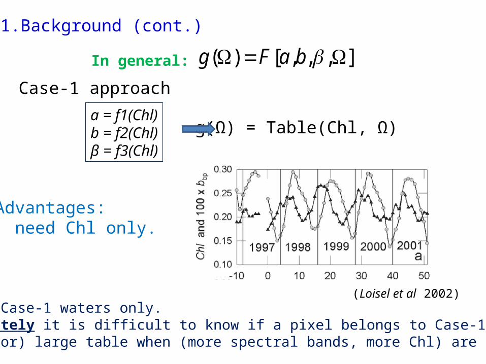
Case-1 approach

a = f1(Chl)b = f2(Chl)β = f3(Chl)

g(Ω) = Table(Chl, Ω)

Caveats: 1. For Case-1 waters only. 2. Remotely it is difficult to know if a pixel belongs to Case-1 or not. 3. (minor) large table when (more spectral bands, more Chl) are required.

Advantages: need Chl only.

],,,[)( baFgIn general:

(Loisel et al 2002)


Objectives of IOP-based BRDF Correction: 1. reduce or minimize the dependency on empirical bio-optical relationships.

2. avoid the Case-1 assumption.

3. coefficients vary with angular geometry only.

bbp [m-1]

rela

tive

dis

trib

utio

n

[%]

0.001 0.01 0.1

0

5

10

15

20

25

440 nm555 nm

2. Decision on particle phase function shape

Locations of VSF measurements

Distribution of bbp (wide range)

2. Decision on particle phase function shape (cont.)

0 50 100 150

1e-1

1e+0

1e+1

1e+2

1e+3

1e+4

1e+5

1e+6

80 100 120 140 160 180

0.0

0.5

1.0

1.5

2.0

2.5

3.0

Scattering angle [deg]

Pha

se f

unct

ion

norm

aliz

ed a

t 12

0o

Examples of newly measured phase function shape

scattering angle [deg]

1 10 100

120o -n

orm

aliz

ed s

catt

eri

ng

fun

ctio

n (a

t 44

0nm

)

1e+0

1e+1

1e+2

1e+3

1e+4

1e+5

1e+6

GOMBlack SeaAOPEXMont. BayHudson (5)Hudson (11)S. Ocean

scattering angle [deg]

80 100 120 140 160 180

120o -n

orm

aliz

ed s

catt

erin

g fu

nctio

n (a

t 44

0 nm

)

0.5

1.0

1.5

2.0

2.5

3.0

GOMBlack SeaAOPEXMont. BayHudson (5)Hudson (11)S. Ocean


Cruise average of measured shape

They are not the same!But very similar.

rela

tive

dis

trib

utio

n

[%]

β(160o)/β(120o)0.0 0.5 1.0 1.5 2.0 2.5 3.0

0

10

20

30

40

440 nm555 nm

bbp [m-1]

rela

tive

dis

trib

utio

n

[%]

0.001 0.01 0.1

0

5

10

15

20

25

440 nm555 nm


Distribution of the shapes

Apparently there is a dominant appearance for wide range of bbp!

0 20 40 60 80 100 120 140 160 180

1e-1

1e+0

1e+1

1e+2

1e+3

1e+4

1e+5

1e+6

1e+7

Petzold avgnew avg

80 100 120 140 160 180

0.0

0.5

1.0

1.5

2.0

2.5

3.0


An average shape is determined from the measurements


Pha

se f

unct

ion

norm

aliz

ed a

t 12

0o

θS

ψ

θv

Lw(Ω)

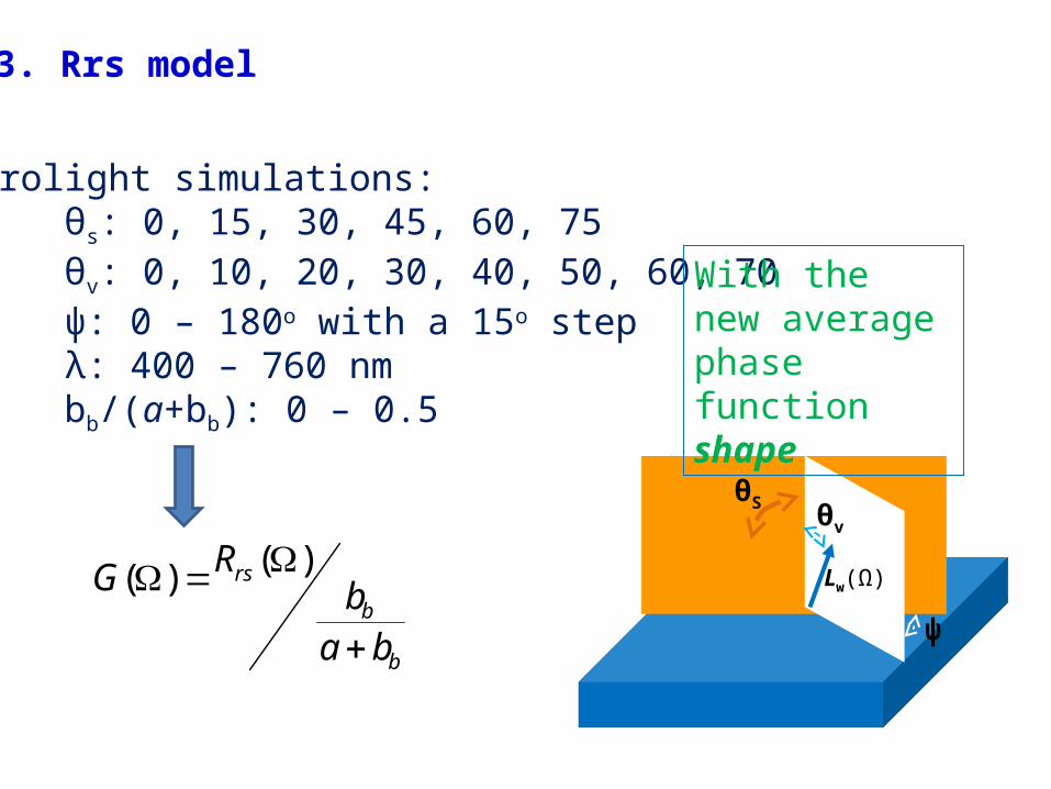
3. Rrs model

Hydrolight simulations: θs: 0, 15, 30, 45, 60, 75 θv: 0, 10, 20, 30, 40, 50, 60, 70 ψ: 0 – 180o with a 15o step λ: 400 – 760 nm bb/(a+bb): 0 – 0.5

b

b

rs

bab

RG

)()(

With the new average phase function shape

3. Rrs model (cont.)

)()()( gG

(Gordon 2005)

Model parameters for g[Ω] are also available.

Note: This G includes the cross-surface effect and the subsurface model parameter.

bb/(a+bb)

G f

rom

HL

sim

ulat

ion

[sr

-1]

(Ω: 60,40,90)

1. G is not a monotonic function of bb/(a+bb)2. G flats out when bb/(a+bb) gets large (saturation)

3. Rrs model (cont.): Example of G parameter variation

b

b

ba

bGGG

)()()( 10

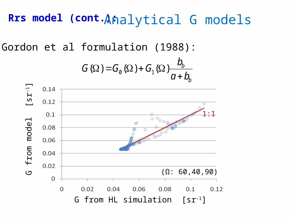
3. Rrs model (cont.):

Gordon et al formulation (1988):

Analytical G models

G from HL simulation [sr-1]

G fr

om

mo

del

[sr

-1]

1:1

(Ω: 60,40,90)

Other formulations

Van Der Woerd and Pasterkamp (2008)


4

1

),()(i

i

b

bbirs ba

bGR

4

1

4

0

)ln()ln()()(lnj

jiij

irs baPR

4

1

),,()(i

i

b

bivSrs ba

bpwqR

Albert and Mobley (2003)

Park and Ruddick (2005)

1. Not resolving the non-monotonic dependency (contribution of molecular scattering)2. High-order polynomials do not behave smoothly outside the range …

Caveats:

Lee et al (2004)

b

bp

b

bpppp

b

bwwrs ba

b

ba

bGGG

ba

bGR

)(exp()(1)()()( 210


Cannot invert a&bb algebraically.Caveats:


G fr

om

mo

del

[sr

-1]

1:1

(Ω: 60,40,90)

G ~ 0.07

Rrs443 [sr-1]

b

bp

b

bppp

b

bwwrs ba

b

ba

bGG

ba

bGR

)()()()( 10


A practical choice for algebraic inversion

Global distribution of Rrs(443)


G f

rom

mod

el

[sr-1

]

1:1

(Ω: 60,40,90)

0.04 0.05 0.06 0.07 0.08 0.09 0.10 0.11 0.12

0.0004

0.0006

0.0008

0.0010

0.0012

0.0014

0.0016

0.0018

Huot 2008No-separationAfter separation

Chl [mg/m3]

b bp(

555)

[m

-1]

After the separation of molecular and particle scatterings on the model parameter, derived bbp compared much better with in situ measurements.


Retrieved Chl and bbp(555) of North Pacific Gyre (from SeaWiFS)

Distribution of Rrs difference between 0 m/s and 10 m/sdi

strib

utio

n

94.4% within 5%!

Impact of wind speed


impact of wind speed is small (consistent with earlier studies).

Difference =2/)( 21

21

wrs

wrs

wrs

wrs

RR

RR

Table ((7x13+1)x4x6) array, 2208 elements) of {G(Ω)}

0.0593 0.0584 0.0586 0.0585 0.0588 0.0583 0.0586 0.0583 …0.012 0.0177 0.0177 0.0176 0.0176 0.0163 0.0169 0.0131 …

0.0529 0.0502 0.0504 0.0503 0.0506 0.0502 0.0504 0.05 …0.1277 0.1402 0.14 0.14 0.1404 0.1392 0.1398 0.1397 …0.0581 0.0601 0.06 0.0598 0.06 0.059 0.0587 0.0577 …0.0178 0.0157 0.0177 0.0176 0.0113 0.0123 0.0146 0.0178 …0.0483 0.0527 0.0525 0.0514 0.0504 0.0489 0.0482 0.047 …0.1511 0.1324 0.1342 0.138 0.1445 0.1481 0.1535 0.1569 …0.0575 0.0598 0.0599 0.0598 0.0596 0.0584 0.0581 0.057 …0.0178 0.0176 0.0176 0.0123 0.0137 0.0178 0.0158 0.0179 …0.0463 0.0506 0.0505 0.0496 0.0488 0.0474 0.0466 0.0455 …0.1642 0.1438 0.1456 0.1488 0.1547 0.1578 0.165 0.1709 …

… … … … … … … … …

(if based on Chl, it is 6x13x7 = 546 elements per band per Chl)

3. Rrs model (cont.)(with 5 m/s wind)

Angular-dependent model coefficients for Rrs(Ω) are now available.

4. IOP-centered BRDF correction & validation

Rrs(Ω) {a&bb} G[0] Rrs[0]

IOP approach

QAA, optimization, linear matrix, etc.

Algebraic algorithm (e.g., QAA, linear matrix)(Lee et al. 2002, Hoge and Lyon 1996)

Y

bb

0

0bpbp )()(

Rrs()

)()()( 00w0 aaa

)(),(),(F)( 0bw0020bp baRb rs

)(),(),(F)( bwbp3 bbRa rs

Y

4. IOP-centered BRDF correction & validation (cont.)

Optimization algorithm (e.g. GSM01, HOPE)

(Roesler and Perry 1996, Lee et al. 1996, Maritorena et al. 2001)

)}({)}({)()( 21w dgph aFaFaa

)}({)()( 3bw bpb bFbb

bpbwrs bbaFR ,,

),,(modbpbwrs bbaFR

)( modrs

mears RRFerror

.0 onoptimizatiRrs.0 QAARrsInput-model focusInput-data focus


0.01 0.1 1

0.01

0.1

1

Known a [m-1]

Der

ived

a

from

Rrs(Ω

) [m

-1]

0.0001 0.001 0.01 0.1

0.0001

0.001

0.01

0.1

Known bbp [m-1]

Der

ived

bbp

fr

om R

rs(Ω

) [m

-1]

HL simulated data: Sun at 60o, 10-70o view angles and 0-180o azimuth Wavelength: 400 – 760 nm

Comparison of IOPs (via QAA)

Retrieval and correction examples

Before correction: 63% & 38% are within 10% and 5%, respectively.After correction: 99% & 95% are within 10% and 5%, respectively

0 10 20 30 40 50

0

10

20

30

40

50

60

before BRDF correctionafter BRDF corrrection

Dis

trib

utio

n [%

]

100]0[

]0[]0[

known

rs

knownrs

derivedrs

R

RR


Comparison of Rrs[0]

Dis

trib

utio

n [

%]

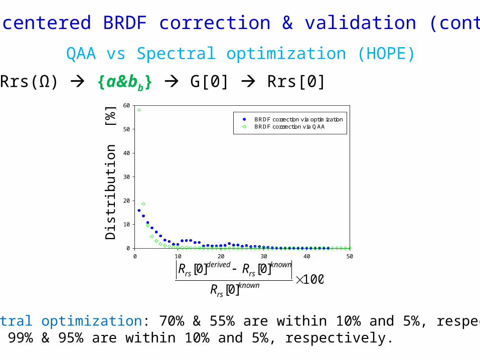
Via spectral optimization: 70% & 55% are within 10% and 5%, respectively.Via QAA: 99% & 95% are within 10% and 5%, respectively.


0 10 20 30 40 50

0

10

20

30

40

50

60

BRDF correction via optimizationBRDF corrrection via QAA

QAA vs Spectral optimization (HOPE)

Rrs(Ω) {a&bb} G[0] Rrs[0]

100]0[

]0[]0[

known

rs

knownrs

derivedrs

R

RR

0.0001 0.001 0.01

0.0001

0.001

0.01

0.01 0.1 1

0.01

0.1

1

0.00 0.02 0.04 0.06 0.08 0.10

0.00

0.02

0.04

0.06

0.08

0.10

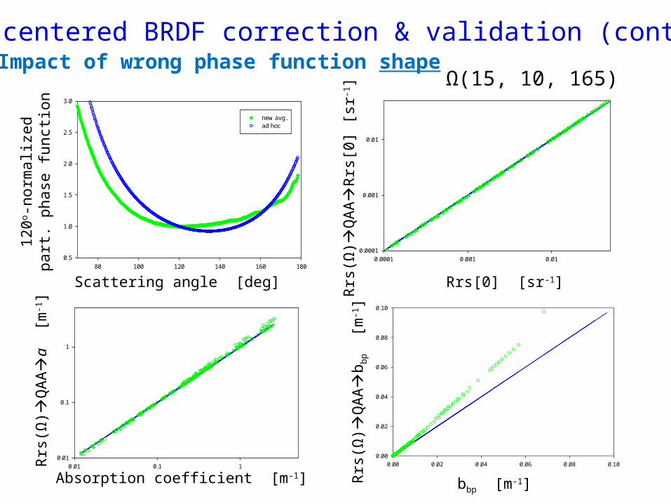
4. IOP-centered BRDF correction & validation (cont.)Impact of wrong phase function shape

80 100 120 140 160 180

0.5

1.0

1.5

2.0

2.5

3.0

new avg.ad hoc

Ω(15, 10, 165)


120o -

norm

aliz

edpa

rt. p

hase

func

tion

Absorption coefficient [m-1]

Rrs

(Ω)

QA

A

a [

m-1]

Rrs[0] [sr-1]

Rrs

(Ω)

QA

A

Rrs

[0] [

sr-1]

Rrs

(Ω)

QA

A

b bp

[m-1]

bbp [m-1]

Wavelength [nm]

400 500 600 700 800

Rrs

[s

r-1 ]

0.000

0.002

0.004

0.006

0.008

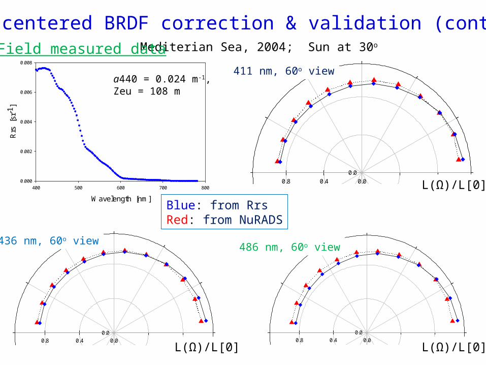
a440 = 0.024 m-1,Zeu = 108 m

Mediterian Sea, 2004; Sun at 30o

4. IOP-centered BRDF correction & validation (cont.)Field measured data

Blue: from RrsRed: from NuRADS

0.00.40.8

0.0

0.4

0.8

Col 2 vs Col 1 Col 5 vs Col 1 Col 35 vs Col 1

411 nm, 60o view

L(Ω)/L[0]

0.00.40.8

0.0

0.4

0.8

L(Ω)/L[0]0.00.40.8

0.0

0.4

0.8

436 nm, 60o view

L(Ω)/L[0]

486 nm, 60o view

Mont. Bay 20060915; Sun at 60o


Wavelength [nm]

400 500 600 700 800

Rrs

[s

r-1 ]

0.000

0.001

0.002

0.003

0.004

0.005

0.006

Blue: from RrsRed: from NuRADSBlack: Hydrolight

a440 = 1.1 m-1,Zeu = 6.8 m

0.00.40.81.21.6

0.0

0.4

0.8

1.2

1.6

411 nm, 60o view

L(Ω)/L[0]

0.00.40.81.21.6

0.0

0.4

0.8

1.2

1.6

436 nm, 60o view

L(Ω)/L[0]


Remote-sensing domain

5. Summary

A. Angular distribution of remote-sensing reflectance (Rrs) highly depends on particle phase function shape (PPFS).

B. PPFS is not a constant, but generally varies within a limited range. An average PPFS (and particle phase function) is derived based on recent measurements.

C. Without known PPFS precisely, BRDF correction is an approximation.

D. The model parameter for Rrs is not a monotonic function of bb/(a+bb). Separating the angular effects of molecule and particle scatterings are important for deriving particle scattering coefficient in oceanic waters.

5. Summary (cont.)

E. Models and procedures to derive IOPs from angular Rrs, and then to correct the angular dependence, are now developed. This approach can be applied to both multi-band and hyperspectral data, and not need to assume Case-1 waters.

F. Excellent results (99% are within 10% error after BRDF correction) are achieved with HL simulated data.

G. Reasonable results are achieved with field measured data, but more tests/evaluation are necessary.

H. Impacts of wrongly assumed PPFS are mainly on the retrieval of particle backscattering coefficient, with minor impact on the retrieval of absorption coefficient. The total absorption coefficient is the least affected parameter from angles/PPFS!

Thank you!

(Mobley et al 2002)


0 10 20 30 40 50 60

0

10

20

30

40

Δβ [%]

Dis

trib

utio

n [

%]

(compared with average shape)

Measurement of shape difference

548 nm, 60o view

AOPEX 081404; Sun at 70o

Wavelength [nm]

400 500 600 700 800

Rrs

[s

r-1]

0.000

0.002

0.004

0.006


486 nm, 60o view

Blue: from RrsRed: from NuRADS

a440 = 0.035 m-1,Zeu = 82 m

rrs modeling and brdf correction zhongping lee 1, bertrand lubac 1, deric gray 2, alan weidemann 2,...

Documents