s emiactive d amping of s tay c ables - university of...
TRANSCRIPT
Semiactive Damping of Stay Cables 1
S
EMIACTIVE
D
AMPING
OF
S
TAY
C
ABLES
By Erik A. Johnson,
1
Associate Member, ASCE, Greg A. Baker,
2
B.F. Spencer, Jr.,
3
Member, ASCE, and Yozo Fujino,
4
Member, ASCE
A
BSTRACT
:
Stay cables, such as are used in cable-stayed bridges, are prone to vibration due to their lowinherent damping characteristics. Transversely-attached passive viscous dampers have been implementedin many bridges to dampen such vibration. Several studies have investigated optimal passive linear viscousdampers; however, even the optimal passive device can only add a small amount of damping to the cablewhen attached a reasonable distance from the cable/deck anchorage. This paper investigates the potentialfor improved damping using semiactive devices. The equations of motion of the cable/damper system arederived using an assumed modes approach and a control-oriented model is developed. The control-ori-ented model is shown to be more accurate than other models and facilitates low-order control designs. Theeffectiveness of passive linear viscous dampers is reviewed. The response of a cable with passive, activeand semiactive dampers is studied. The response with a semiactive damper is found to be dramaticallyreduced compared to the optimal passive linear viscous damper for typical damper configurations, thusdemonstrating the potential benefits using a semiactive damper for absorbing cable vibratory energy.
INTRODUCTION
Long steel cables, such as are used in cable-stayed bridges and other structures, are prone tovibration induced by the structure to which they are connected and by weather conditions. In par-ticular, light-to-moderate wind combined with light-to-moderate rain has been observed to inducesignificant cable motion in cables of various cable-stayed bridges; this phenomenon is generallytermed “rain-wind induced vibration” (
e.g.
, Hikami 1986; Hikami and Shiraishi 1988; Matsumoto1998; Main and Jones 1999). The extremely low damping inherent in such cables, typically onthe order of a fraction of a percent (Yamaguchi and Fujino 1998), is insufficient to eliminate thisvibration, causing reduced cable and connection life due to fatigue and/or breakdown of corrosionprotection (Watson and Stafford 1988; Poston 1998), as well as the risk of losing public confi-dence in such structures.
Several methods have been proposed and/or implemented to mitigate this problem, thougheach has its limitations (
e.g.
, Yamaguchi and Fujino 1998). Tying multiple cables together is asensible approach, but detracts from the aesthetics of the bridge. Changes to cable roughness orother aerodynamic measures have been effective only for certain classes of vibration, are difficultto implement for retrofit, and have disadvantages at high wind velocities. Active transverse and/oraxial control of cable vibration (
e.g.
, Fujino
et al.
1993; Yamaguchi and Dung 1992) may requirepower sources beyond practical limits, given the number of cables on a typical cable-stayedbridge and the isolated locations at which they are often placed. Discrete passive viscous dampersattached perpendicular to the cables have been used on a number of bridges, such as the BrotonneBridge in France (Gimsing 1983), the Sunshine Skyway Bridge in Florida (Watson and Stafford
1. Assoc. Prof., Dept. of Civil Engrg., Univ. of Southern California, Los Angeles, CA 90089. [email protected] 2. Formerly, Grad. Rsrch. Asst., Dept. of Civil Engrg. & Geo. Sci., Univ. of Notre Dame, IN 46556.3. Newmark Endowed Chair in Civil Engineering, Univ. of Illinois, Urbana IL 61801 [email protected] 4. Prof., Dept. of Civil Engrg., University of Tokyo, Bunkyo-ku, Tokyo 113, Japan. [email protected]
Key words: smart damping, stay cables, structural control, semiactive dampers, rain-wind induced vibration
ASCE
Journal of Engineering Mechanics
,
133
(1), 2007.This draft version at http://rcf.usc.edu/~johnsone/papers/smartdamping_tautcable_jem.html
Semiactive Damping of Stay Cables 2
1988) and the Aratsu Bridge in Japan (Yoshimura
et al.
1989), though the damper attachmentlocation is typically restricted to be within 5% (of the cable length) from the cable anchorage.
For an attached discrete linear viscous damper, it has been demonstrated (
e.g.
, Kovacs 1982;Sulekh 1990; Pacheco
et al.
1993; Krenk 2000) that an optimal damper size exists for a givencable configuration. This is easily understood when one considers that approaching a zerodamping constant in the viscous damper, the cable vibrates nearly unimpeded, and approaching aninfinite damping constant, the cable again vibrates nearly unimpeded but in the span beyond thelocation of the attached damper; the optimum, then, must fall somewhere in between. Fujino andcolleagues (Sulekh 1990; Pacheco
et al.
1993) derived an approximate relationship that may beused to estimate the optimal damper design for a given cable configuration and attachment loca-tion.
Several studies (
e.g.
, Kovacs 1982; Pacheco
et al.
1993; Krenk 2000; Main and Jones 2002a)have shown that the maximum amount of damping added to the cable with a transverse passivelinear damper is approximately proportional to the distance, relative to the cable length, betweenthe damper and the cable/deck anchorage. Similar damping levels are also achieved by nonlinearpassive dampers (Main and Jones 2002b; Krenk and Høgsberg 2005). Further, any device rigidityreduces passive damper performance and while adding mass can increase damping (Krenk andHøgsberg 2005), it is still likely to be on the same order as that of a linear passive damper.Modern cable-stayed bridges are using longer and longer cables, such as cables on the Tatara andNormandie Bridges which are more than 450 meters long (Endo
et al.
1991; Virloguex
et al.
1994) (a planned 1100 meter main-span bridge in Hong Kong (Russell 1999) would require evenlonger stay cables). With such long cables, approaching a 5% connection point may be infeasiblewithout significant changes to the aesthetics of the structure. Rather, a 1% to 2% location is morelikely. In such a case, passive dampers may add insufficient damping to the cables. Therefore,other methods of mitigating excessive cable vibration must be explored.
Semiactive dampers, whether of the variable orifice, controllable friction, or controllablefluid varieties, have proven to be of significant interest in many applications (Housner
et al.
1997;Spencer and Sain 1997) and can potentially achieve performance levels nearly the same as compa-rable active devices with few of the detractions. This paper investigates the efficacy of employinga semiactive damper as an alternative to a transverse passive viscous damper for reducing cablemotion. It will be demonstrated via simulation that a semiactive device may provide dramaticreductions in cable response over the optimal linear viscous damper and achieve nearly the sameperformance as a comparable active damper.
CABLE DYNAMICS
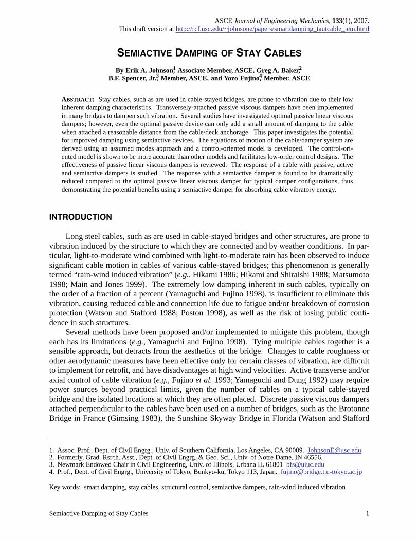
Stay cables typically have small sag (on the order of 1% sag-to-length ratio) with hightension-to-weight ratios. With small sag, the inclination, the static deflection due to gravity, andthe flexural rigidity may be neglected since they are second order effects. Consequently, themotion of the cable may be modeled by the motion of a taut string (Irvine 1981). Consider thetransverse motion of a
cable with a damper attached transverse to the cable as shown in Fig. 1.For small deflection, this system has the following nondimensional partial differential equation ofmotion
Semiactive Damping of Stay Cables 3
, (1)
with boundary conditions
for all
t
(2)
where is the transverse deflection of the cable, is the viscous damping per unit length, and denote partial derivatives with respect to and , respectively, is the distrib-
uted load on the cable, is a transverse damper force at location , and is the Diracdelta function. The nondimensional quantities are related to their dimensional counterparts,shown with overbars, according to the following relations
(3)
where
L
is the length of the cable, is the fundamental natural frequency of the undampedcable,
T
is the cable tension, and is the cable mass per unit length. (Note that, unless otherwisespecified, all quantities in the remainder are nondimensional.)
The excitation is assumed to be a stochastic process. For convenience, assume theexcitation may be approximated by
(4)
where the are deterministic functions of position along the cable and the are the com-ponents of a stationary, ergodic, zero-mean stochastic vector process.
Approximation using Series
The transverse deflection may be approximated using a finite series
(5)
Figure 1: Cable with Attached Damper (parameters here are dimensional).
L
xdT, ρ, c
F (t)d
v(x,t)
x-
---
- - -
-
v̇̇ x t,( ) cv̇ x t,( ) 1π2-----v″ x t,( )–+ f x t,( ) Fd t( )δ x xd–( )+= 0 x 1≤ ≤
v 0 t,( ) v 1 t,( ) 0= =
v x t,( ) c ( )′ ̇( ) x t f x t,( )
Fd t( ) x xd= δ ·( )
t ω0t= x x L⁄= c c ρω0⁄= v x t,( ) v x t,( ) L⁄= ω02 T π2 ρL2⁄=
δ x xd–( ) Lδ x xd–( )= f x t,( ) L f x t,( ) π2T⁄= Fd t( ) Fd t( ) π2T⁄=
ω0ρ
f x t,( )
f x t,( ) αi x( )βi t( )i 1=
n
∑=
αi x( ) βi t( )
v x t,( ) qj t( )φj x( )j 1=
m
∑=
Semiactive Damping of Stay Cables 4
where the are generalized displacements and the are a set of shape functions that arecontinuous with piecewise continuous slope and that satisfy the geometric boundary conditions
. Substituting (5) into the nondimensional equation of motion (1), using astandard Galerkin approach (Craig 1981) (i.e., assume the truncation error is orthogonal to theshape functions retained), multiplying by and integrating over the length of the cable gives
(6)
(7)
with mass , damping , and stiffness matrices, generalized dis-placement vector , externally applied load vector ,and damper load vector .
Solution by Sine Series Approximation
Pacheco et al. (1993) assumed sinusoidal shape functions, , identical to themode shapes of the cable without the damper, to compute the damping with attached viscousdampers. Since these sinusoidal shape functions are mutually orthogonal, the mass, damping andstiffness matrices are diagonal. Using a linear viscous damper, , the cable/damper system may be posed in state space form as
(8)
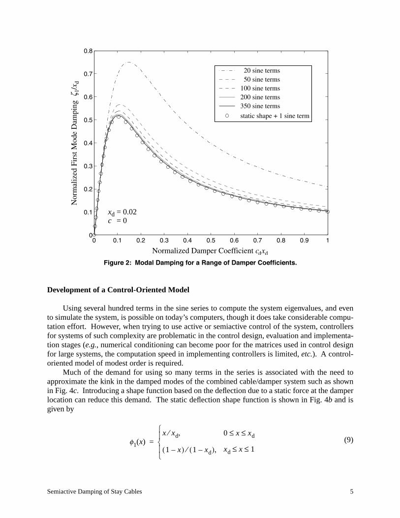
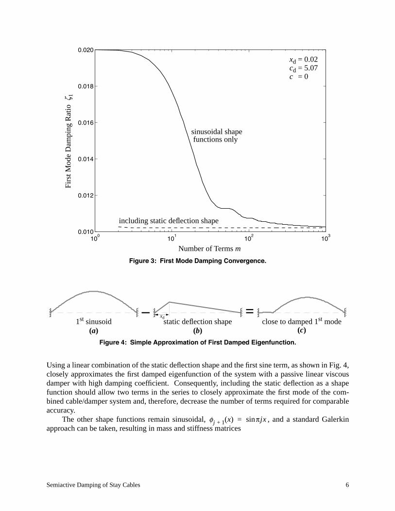
where is the Kronecker delta. (Note: the cd used here is nondimensional; the correspondingdimensional term is given by .) A simple eigenvalue analysis of the state matrix in(8) may be used to compute the damping in the system. Figure 2 shows the normalized modaldamping as a function of the damper coefficient cd; this particular graph was generated using thefirst mode with a damper location xd = 0.02, but is similar for other damper locations and othermodes (Pacheco et al. 1993). Additionally, the inherent cable damping c was assumed here to bezero; typical values of c for real cables are sufficiently small that the graph would change insignif-icantly. Two important observations may be drawn from Fig. 2. First, there is a linear viscousdamper that maximizes the damping in the first mode, as was observed in a number of previousstudies (e.g., Kovacs 1982; Sulekh 1990; Pacheco et al. 1993). Second, as was also noted byPacheco et al. (1993), the number of terms required to accurately compute the optimal damping isquite large. This observation may also be seen in Fig. 3, which shows the computed value of ζ1,the damping ratio in the first mode, as a function of the number of terms used in the series approx-imation for the optimal damper coefficient (cd = 5.07) at location xd = 0.02. The series using sinu-soidal shape functions converges rather slowly, requiring hundreds of shape functions forconvergence of ζ1.
qj t( ) φj x( )
φj 0( ) φj 1( ) 0= =
φi x( )
mij φi x( )φj x( ) xd0
1
∫= cij c φi x( )φj x( ) xd0
1
∫=
kij1π2----- φi
′ x( )φj′ x( ) xd
0
1
∫= fi t( ) f x t,( )φi x( ) xd0
1
∫=
Mq̇̇ Cq̇ Kq+ + f ϕϕϕϕ Fd t( )+=
M mij[ ]= C cij[ ]= K kij[ ]=q qi t( )[ ]= f f t( ) f1 f2 … fm[ ]T= =
ϕϕϕϕ φφφφ xd( ) φ1 xd( ) φ2 xd( ) … φm xd( )[ ]T= =
φi x( ) πixsin=
Fd t( ) c– dv̇ xd t,( )=
q̇
q̇̇⎩ ⎭⎨ ⎬⎧ ⎫ 0 I
i2δij[ ]– cI– 2cdϕϕϕϕϕϕϕϕT–
q
q̇⎩ ⎭⎨ ⎬⎧ ⎫ 0
2If+=
δijcd ρω0Lcd=
Semiactive Damping of Stay Cables 5
Development of a Control-Oriented Model
Using several hundred terms in the sine series to compute the system eigenvalues, and evento simulate the system, is possible on today’s computers, though it does take considerable compu-tation effort. However, when trying to use active or semiactive control of the system, controllersfor systems of such complexity are problematic in the control design, evaluation and implementa-tion stages (e.g., numerical conditioning can become poor for the matrices used in control designfor large systems, the computation speed in implementing controllers is limited, etc.). A control-oriented model of modest order is required.
Much of the demand for using so many terms in the series is associated with the need toapproximate the kink in the damped modes of the combined cable/damper system such as shownin Fig. 4c. Introducing a shape function based on the deflection due to a static force at the damperlocation can reduce this demand. The static deflection shape function is shown in Fig. 4b and isgiven by
(9)
0 0.1 0.2 0.3 0.4 0.5 0.6 0.7 0.8 0.9 10
0.1
0.2
0.3
0.4
0.5
0.6
0.7
0.8
Normalized Damper Coefficient cdxd
Nor
mal
ized
Fir
st M
ode
Dam
ping
ζ1/
x d 20 sine terms 50 sine terms100 sine terms200 sine terms350 sine terms
static shape + 1 sine term
Figure 2: Modal Damping for a Range of Damper Coefficients.
xd = 0.02 c
d = 0
φ1 x( )x xd⁄ , 0 x xd≤ ≤
1 x–( ) 1 x– d( )⁄ , xd x 1≤ ≤⎩⎪⎨⎪⎧
=
Semiactive Damping of Stay Cables 6
Using a linear combination of the static deflection shape and the first sine term, as shown in Fig. 4,closely approximates the first damped eigenfunction of the system with a passive linear viscousdamper with high damping coefficient. Consequently, including the static deflection as a shapefunction should allow two terms in the series to closely approximate the first mode of the com-bined cable/damper system and, therefore, decrease the number of terms required for comparableaccuracy.
The other shape functions remain sinusoidal, , and a standard Galerkinapproach can be taken, resulting in mass and stiffness matrices
100
101
102
103
0.010
0.012
0.014
0.016
0.018
0.020
Number of Terms m
Firs
t Mod
e D
ampi
ng R
atio
ζ1
Figure 3: First Mode Damping Convergence.
x
d = 0.02
sinusoidal shape
including static deflection shape
c
d = 5.07 c
d = 0
functions only
Figure 4: Simple Approximation of First Damped Eigenfunction.
– =1st sinusoid close to damped 1st modestatic deflection shape
(a) (b) (c)
xd
φj 1+ x( ) πjxsin=
Semiactive Damping of Stay Cables 7
(10)
and damping matrix . The state-space representation can be formulated as
(11)
where is the state vector, is a vector of quantities to be reg-ulated (includes the generalized displacements, velocities, and terms related tothe generalized accelerations), is a vector of noisy sensor measure-ments (includes the displacement and acceleration at the damper location), is a vector of sto-chastic sensor noise processes, and
(12)
Assessment of Control-Oriented Cable Model
A control-oriented model of the cable should, with only a few terms, adequately describe thedynamic characteristics of the cable, including the natural frequency
ω
i
, damping ratio
ζ
i
, andeigenfunction for each mode. To investigate the convergence rate for the two series approx-imations, consider the passive linear viscous damper located at
x
d
= 0.02 that maximizes thedamping in the first mode (
i.e.
,
c
d
= 5.07). Figure 3 shows that the damping in the first mode con-verges
very
fast when using the static deflection shape compared to without it. In fact, the relativeerror in the damping estimate computed using only the static deflection shape and the first sinu-soid is less than 0.001, compared to over 1000 sinusoids alone for the same accuracy. Similartrends occur for higher modes as well.
M[ ]ij
12---δij , i > 1 j > 1,
13--- , i = 1 j = 1,
kπxdsin
xd 1 xd–( )k2π2------------------------------------ , otherwise
where k = max i j,{ } 1–⎩⎪⎪⎪⎪⎨⎪⎪⎪⎪⎧
= K[ ]ij
12--- i 1–( )2δij , i > 1 j > 1,
1xd 1 xd–( )π2------------------------------ , i = 1 j = 1,
kπxdsin
xd 1 xd–( )π2------------------------------ , otherwise
where k = max i j,{ } 1–⎩⎪⎪⎪⎪⎨⎪⎪⎪⎪⎧
=
C cM=
ηηηη̇ = Azηηηη + BzFd t( ) + Gzf
z = Czηηηη + DzFd t( ) + Hzf
y = Cyηηηη + DyFd t( ) + Hyf + v
ηηηη qT q̇T[ ]T= z qT q̇T q̇̇˜
T[ ]T=q̇̇˜
q̇̇ M 1– f–=y v xd t,( ) v̇̇ xd t,( )[ ]T v+=
v
Az 0 I
M 1– K– M 1– C–
= Bz 0
M 1– ϕϕϕϕ
= Gz 0
M 1–
=
Cz
I 0
0 I
M 1– K– M 1– C–
= Dz
0
0
M 1– ϕϕϕϕ
= Hz
0
0
0
=
CyϕϕϕϕT 0
ϕϕϕϕTM 1– K– ϕϕϕϕTM 1– C–= Dy
0
ϕϕϕϕTM 1– ϕϕϕϕ= Hy
0
ϕϕϕϕTM 1–=
φ̃i x( )
Semiactive Damping of Stay Cables 8
A second test of the convergence of the cable model is to examine the convergence of thedamping as a function of the viscous damper coefficient. Figure 2 shows the normalized modaldamping with and without the static deflection shape function for several numbers of terms in theseries. Again, including the static deflection shape allows the same accuracy with only a fewterms as would be attained with hundreds of terms in the sine-only series.
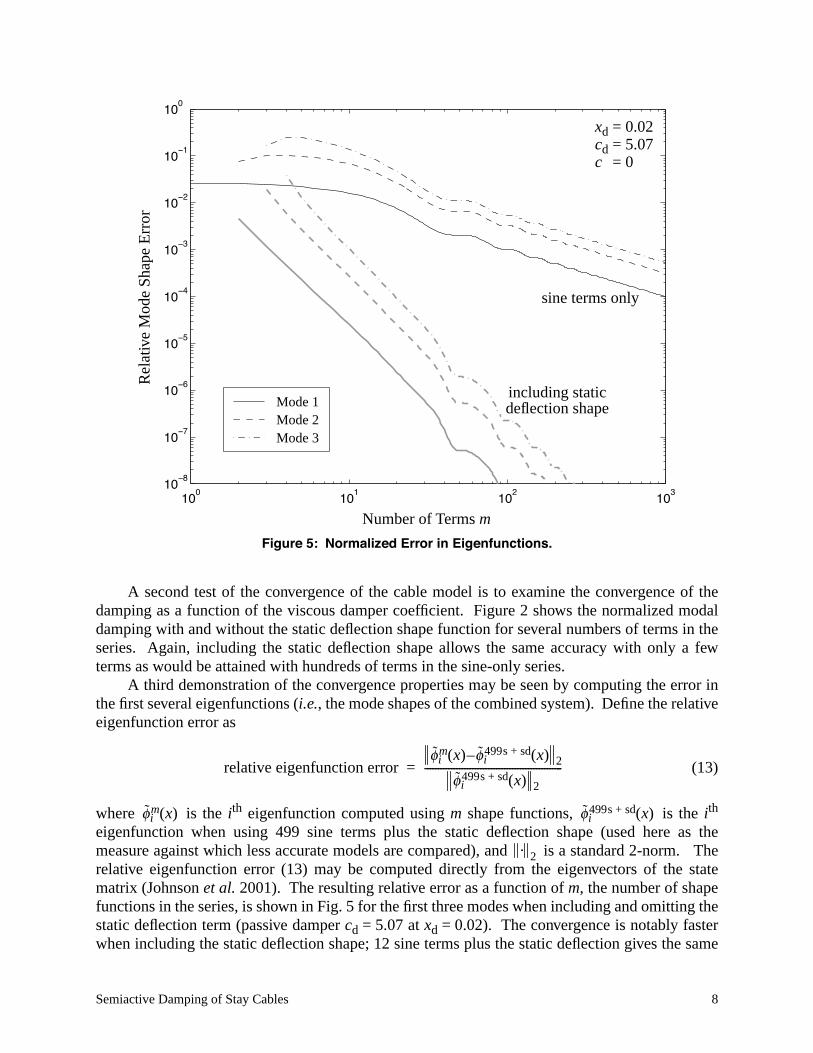
A third demonstration of the convergence properties may be seen by computing the error inthe first several eigenfunctions (i.e., the mode shapes of the combined system). Define the relativeeigenfunction error as
(13)
where is the ith eigenfunction computed using m shape functions, is the ith
eigenfunction when using 499 sine terms plus the static deflection shape (used here as themeasure against which less accurate models are compared), and is a standard 2-norm. Therelative eigenfunction error (13) may be computed directly from the eigenvectors of the statematrix (Johnson et al. 2001). The resulting relative error as a function of m, the number of shapefunctions in the series, is shown in Fig. 5 for the first three modes when including and omitting thestatic deflection term (passive damper cd = 5.07 at xd = 0.02). The convergence is notably fasterwhen including the static deflection shape; 12 sine terms plus the static deflection gives the same
relative eigenfunction errorφ̃i
m x( ) φ̃i499s sd+ x( )– 2
φ̃i499s sd+ x( ) 2
----------------------------------------------------=
φ̃im x( ) φ̃i
499s sd+ x( )
· 2
100
101
102
103
10−8
10−7
10−6
10−5
10−4
10−3
10−2
10−1
100
Number of Terms m
Rel
ativ
e M
ode
Shap
e E
rror
Mode 1 Mode 2 Mode 3
Figure 5: Normalized Error in Eigenfunctions.
including staticdeflection shape
sine terms only
xd = 0.02 c
d = 5.07 c
d = 0
Semiactive Damping of Stay Cables 9
accuracy as 1000 sine terms alone for the first three eigenfunctions. Similar trends exist forhigher modes as well.
Thus, using the static deflection shape function will provide a low-order control-orientedmodel with accuracy sufficient to capture the salient dynamics of the combined cable/dampersystem.
CONTROL OF CABLE VIBRATION
Three types of dampers are considered in this study. The damper of primary interest is ageneral semiactive device, one that may exert any required
dissipative
force. However, compari-son with passive linear viscous dampers, similar to the oil dampers that have been installed innumerous cable-stayed bridges, is vital to demonstrate the improvements that may be possiblewith semiactive damping technology. Additionally, comparison with active control devices isuseful as they bound the achievable performance.
Passive Viscous Damper
If the damping device is a passive linear viscous damper, then the damper force is where is a nondimensional damping constant and is the nondi-
mensional velocity at the damper location . The resulting state-space equations are
(14)
where
(15)
As noted above, the modal damping may be determined for this system via a straightforwardeigenvalue analysis. When the distributed viscous damping is negligible, which is typically thecase for long stay cables, Fig. 2 shows the damping ratio for various levels of viscous damping
. It may be noted that the shape of the curve this curve is similar for higher modes but with thepeak at different locations; consequently, the optimal choice of is different for maximizing themodal damping for different modes of the combined system.
Alternate Measures of Damper Performance
Modal damping ratios provide a useful means of determining the effectiveness of linearviscous damping strategies. However, using a semiactive damper introduces a nonlinearity intothe combined system. Consequently, performance measures other than modal damping must beused for judging the efficacy of nonlinear damping strategies in comparison with linear (passive oractive) dampers.
Fd t( ) cdv̇ xd t,( )–= cd v̇ xd t,( )v̇ xd t,( ) ϕϕϕϕTq̇ 0T ϕϕϕϕT[ ]ηηηη= =
ηηηη̇ = APηηηη + Gzf
z = CPηηηη + Hzf
AP A 0 0
0 cdM 1– ϕϕϕϕϕϕϕϕT–+= CP Cz
0 00 0
0 cdM 1– ϕϕϕϕϕϕϕϕT–
+=
cdcd
Semiactive Damping of Stay Cables 10
Using the root mean square (RMS) or peak response of the cable at some particular location(or several locations) is one possible measure of damper performance. However, it may be possi-ble for one control strategy to decrease the motion significantly in some regions of a structure butallow other parts to vibrate relatively unimpeded. Thus, the primary measure of damper perfor-mance considered herein is the root mean square (RMS) cable deflection defined by
(16)
The corresponding RMS cable velocity and a term related to the cable acceleration may be com-puted using
(17)
where (i.e., the generalized acceleration minus the effect of the external load). Ofcourse, if the focus is on the stationary response — which is the case herein — then all three ofthese performance measures are constant and not functions of time.
For the linear systems (passive linear viscous dampers and active dampers), these quantitiesmay be computed by solving a Lyapunov equation. For example, if the excitation vector f is azero-mean Gaussian white noise vector process with where isthe spectral density matrix, and the damper is a passive linear viscous damper, maybe computed from (16) where and where is the solu-tion of the Lyapunov equation .
Active Damper
The optimal passive viscous damper provides one benchmark against which to judge semi-active dampers. The other end of the spectrum of control possibilities is an ideal active damper,which may exert any desired force. The performance of the actively controlled systems give aperformance target for semiactive control.
Four LQR (linear quadratic regulator) control designs are considered in this study. Thesestate feedback controllers use force proportional to the state of the system, ,where is the feedback gain that minimizes one of four cost functions. The first controller,using cost , weights the cable displacement , the second the velocity , thethird a combination of displacement and velocity , and the fourth a term
related to the acceleration. These cost functions can be written in general form
, (18)
where
σdisplacement
σdisplacement2 t( ) E v2 x t,( ) xd
0
1
∫ trace M1 2/ E q t( )qT t( )[ ]M1 2/{ }= =
σvelocity2 t( ) E q̇T t( )Mq̇ t( )[ ] trace M1 2/ E q̇ t( )q̇T t( )[ ]M1 2/{ }= =
σa2 t( ) E q̇̇
˜T t( )Mq̇̇
˜t( )[ ] trace M1 2/ E q̇̇
˜t( ) q̇̇
˜T t( )[ ]M1 2/{ }= =
q̇̇˜
q̇̇ M 1– f–=
E f t( )fT t τ+( )[ ] 2πS0δ τ( )= S0σdisplacement
E qqT[ ] I 0[ ]ΣΣΣΣ I 0[ ]T= ΣΣΣΣ E ηηηηηηηηT[ ]=APΣΣΣΣ ΣΣΣΣAP
T G2πS0GT+ + 0=
Fdactive t( ) Lkηηηη–=
LkJ1 σdisplacement
2 σvelocity2
12---σdisplacement
2 12---σvelocity
2+σa
2
Jk E1T--- zTQkz R Fd
2+( ) td0
T
∫T ∞→lim= k 1 2 3 4, , ,=
Semiactive Damping of Stay Cables 11
(19)
The feedback gain that minimizes the cost (18) is where satisfies the algebraic Riccati equation
(20)
Varying the control weight R will then give four families of state feedback controllers. Note thatbecause of the certainty equivalence principle (e.g., Stengel 1986), the zero-mean external excita-tion vector drops out of the state feedback control design.
Of course, it is unreasonable to assume that one has perfect full state information for a cablesystem. Consequently, some of the designs in this study use a Kalman filter to estimate the statesof the system based on (noisy) sensor measurements of displacement and acceleration at thedamper location. (These two measurements are likely to be the easiest to use in a full-scale imple-mentation as they could be packaged as a part of the damper system.) The resulting estimator isdynamic with order equal to that of the cable state space model, and is given by
(21)
where is an estimate of the states , , , , is the estimator gain and is computed from
the Riccati equation
(22)
where is the magnitude of the excitation spectral density , the magnitude ofnoise spectral density , , , and excitation and sensor noise areuncorrelated. The force, then, is given by .
Semiactive Damper
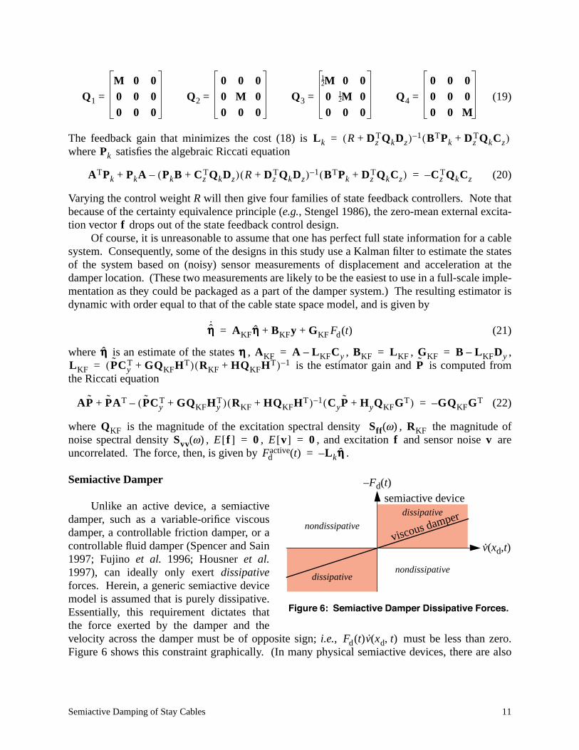
Unlike an active device, a semiactivedamper, such as a variable-orifice viscousdamper, a controllable friction damper, or acontrollable fluid damper (Spencer and Sain1997; Fujino et al. 1996; Housner et al.1997), can ideally only exert dissipativeforces. Herein, a generic semiactive devicemodel is assumed that is purely dissipative.Essentially, this requirement dictates thatthe force exerted by the damper and thevelocity across the damper must be of opposite sign; i.e., must be less than zero.Figure 6 shows this constraint graphically. (In many physical semiactive devices, there are also
Q1
M 0 00 0 0
0 0 0= Q2
0 0 00 M 0
0 0 0= Q3
M 0 00 M 0
0 0 0= 1
2---
12---
Q4
0 0 00 0 0
0 0 M=
Lk R DzTQkDz+( ) 1– BTPk Dz
TQkCz+( )=Pk
ATPk PkA PkB CzTQkDz+( ) R Dz
TQkDz+( ) 1– BTPk DzTQkCz+( )–+ Cz
TQkCz–=
f
ηηηη̇̂ AKFηηηη̂ BKFy GKF Fd t( )+ +=
ηηηη̂ ηηηη AKF A LKFCy–= BKF LKF= GKF B LKFDy–=LKF P̃Cy
T GQKFHT+( ) RKF HQKFHT+( ) 1–= P̃
AP̃ P̃AT P̃CyT GQKFHy
T+( ) RKF HQKFHT+( ) 1– CyP̃ HyQKFGT+( )–+ GQKFGT–=
QKF Sff ω( ) RKFSvv ω( ) E f[ ] 0= E v[ ] 0= f v
Fdactive t( ) Lkηηηη̂–=
–Fd(t)
v(xd,t)viscous damper
semiactive device
.
Figure 6: Semiactive Damper Dissipative Forces.
dissipative
nondissipative
nondissipative
dissipative
Fd t( )v̇ xd t,( )
Semiactive Damping of Stay Cables 12
maximum force levels; this limit is neglected here.) This generic semiactive device model gives afirst approximation of the performance potential possible with smart dampers.
In previous studies of the control of semiactive dampers (e.g., Dyke et al. 1996a,b; Johnsonet al. 1999a,b), a clipped optimal strategy, employing a two-stage control design, has performedwell. The control algorithm considered here falls into this category. The primary controller is oneof the same LQR or LQG control designs used for the active damper. The secondary controller,which accounts for the nonlinear nature of the semiactive device, may be given by
(23)
Primarily, this secondary controller ensures that the control system does not command non-dissi-pative damper forces. Of course, in a physical device (as opposed to simulation), this restriction isenforced by the nature of the device. (However, one would still need a secondary controller forthe physical device since most semiactive devices are not linear in the relationship betweencommand input and force exerted. Herein, it is assumed that as long as the force is dissipative, itcan be commanded directly.)
The second purpose of this secondary controller is to modulate the force, via the function, when the velocity at the damper location is near zero; this is motivated by both physical and
numerical reasons. In simulations with no modulation function, the following scenario oftenoccurs: in one time step, the velocity has changed sign making the desired damper force dissipa-tive, so the damper force is turned on; during the following time step, the large damper forcedrives the velocity back across zero but with the damper force still on and some displacementoccurs so energy is incorrectly dissipated; the damper force is subsequently turned back off,which will make the velocity change sign again in the third time step. This cycle tends to repeatitself, resulting in many narrow but tall dissipation loops that cannot be repeated in a real semi-active device. Essentially, the damper is trying to lock up and make the cable velocity exactlyzero at the damper location. This numerical dissipation can be reduced only by using extremelysmall time steps (on the order of 10–8 natural periods), which renders response simulation compu-tationally intractable. Further, physical semiactive damping devices, such as MR dampers, cannotproduce large damping forces for near-zero velocities (Spencer et al., 1997; Yang et al., 2002).Thus, in this study, the modulation function is used. Large causes toapproach the function, modulating only when the velocity is very small, and requiring anextremely small integration time step again. In contrast, small accommodates larger integrationtime step but can reduce the control effectiveness since it modulates the forces even at largervelocities. An extensive parameter study found that is an acceptable trade off of controlstrategy performance and simulation tractability.
NUMERICAL RESULTS
A series of numerical studies were conducted to compare and contrast semiactive damperperformance with that of optimal passive linear viscous dampers and linear active dampers. Theinherent distributed viscous damping was chosen to be nearly negligible: c = 0.0001 (which, inthe absence of any other damping device, gives a damping ratio of % in the first mode).Using 20 shape functions (19 sine terms plus the static deflection term) gives less than 0.01%
Fd t( )α v̇ xd t,( )( )Fd
active t( ) , Fdactive t( )v̇ xd t,( ) 0<
0 , otherwise⎩⎨⎧
=
α ·( )
α v̇d( ) µv̇dtanh= µ α ·( )sign ·( )
µ
µ 10=
c0.005
Semiactive Damping of Stay Cables 13
error in the first three combined system eigenfunctions (compared to 499 sine terms plus the staticdeflection term), and gave RMS response nearly identical (less than one percent error) to usingmore terms; consequently, all results shown below use these 20 shape functions. A range ofdamper locations was studied; the results discussed here are primarily for but similarbehavior may be observed for other small .
The phenomena that cause rain-wind induced vibration, including the aerodynamic forces,motion of water rivulets, the nonlinear coupling with the cable motion, and so forth, are not wellunderstood (Main and Jones 1999); consequently, there are no well established models of thisbehavior (Scanlon 1999). However, it has been observed that the response tends to be dominatedby the first few modes. Here, the excitation is assumed to be a subset of the series in (4) using justone term
(24)
where is a zero-mean Gaussian white noise process with . In theabsence of a damper, this excitation would result in first-mode response.
The results for the active and passive strategies are computed exactly (eigenvalue analysis formodal parameters and Lyapunov solutions for stationary response). Computing the statistics ofthe response for the semiactive system requires simulation due to the nonlinear nature of semi-active dampers. The RMS responses with a semiactive damper are determined from simulationtime histories (generated using SIMULINK®) of duration 1600 to 4000 periods of the fundamentalmode of the cable alone (systems with less damping require longer time histories for accurate esti-mation of the RMS response). The sensor noise vector is taken to be a zero-mean Gaussianwhite noise vector process with diagonal spectral density magnitude matrix. The magnitudes arechosen such that using band-limited white noise (nondimensional sampling time of 0.01) in thesimulation (for sensor noise and excitation) gives a certain level of RMS error in each of the twosensor signals. Two different noise levels are studied here: 1% RMS sensor noise, typical of whatone might expect in practice, and 10% RMS sensor noise, included to better understand the sensi-tivity of the semiactive damper results to sensor noise.
Damping Ratio for Linear Control Strategies
The damping ratio in the first several modes was computed for the linear strategies, that is,for passive linear viscous dampers and for active dampers with the four state feedback controllaws. Varying the damper coefficient for the passive designs and the control weight for theactive designs results in five families (one passive, four active) of combined cable/damper sys-tems.
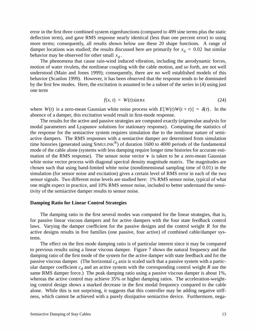
The effect on the first mode damping ratio is of particular interest since it may be comparedto previous results using a linear viscous damper. Figure 7 shows the natural frequency and thedamping ratio of the first mode of the system for the active damper with state feedback and for thepassive viscous damper. (The horizontal cd axis is scaled such that a passive system with a partic-ular damper coefficient cd and an active system with the corresponding control weight R use thesame RMS damper force.) The peak damping ratio using a passive viscous damper is about 1%,whereas the active control may achieve 35% or higher damping ratios. The acceleration-weight-ing control design shows a marked decrease in the first modal frequency compared to the cablealone. While this is not surprising, it suggests that this controller may be adding negative stiff-ness, which cannot be achieved with a purely dissipative semiactive device. Furthermore, nega-
xd 0.02=xd
f x t,( ) W t( ) πxsin=
W t( ) E W t( )W t τ+( )[ ] δ τ( )=
v
R
Semiactive Damping of Stay Cables 14
tive stiffness should tend to increase displacements. Consequently, as will be shown in the nextsection, the acceleration-weighting control design performs poorly in simulations of the semi-active system.
RMS Cable Response
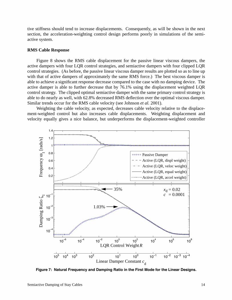
Figure 8 shows the RMS cable displacement for the passive linear viscous dampers, theactive dampers with four LQR control strategies, and semiactive dampers with four clipped LQRcontrol strategies. (As before, the passive linear viscous damper results are plotted so as to line upwith that of active dampers of approximately the same RMS force.) The best viscous damper isable to achieve a significant response decrease compared to the case with no damping device. Theactive damper is able to further decrease that by 76.1% using the displacement weighted LQRcontrol strategy. The clipped optimal semiactive damper with the same primary control strategy isable to do nearly as well, with 62.8% decreased RMS deflection over the optimal viscous damper.Similar trends occur for the RMS cable velocity (see Johnson et al. 2001).
Weighting the cable velocity, as expected, decreases cable velocity relative to the displace-ment-weighted control but also increases cable displacements. Weighting displacement andvelocity equally gives a nice balance, but underperforms the displacement-weighted controller
Linear Damper Constant cd
105 104 103 102 101 100 10−1 10−2 10−3 10−4
10−6
10−4
10−2
100
102
104
106
108
10−4
10−3
10−2
10−1
Dam
ping
Rat
io ζ
1
LQR Control Weight R
0.2
0.4
0.6
0.8
1
1.2
1.4
Freq
uenc
y ω
1 [ra
ds/s
]
Passive Damper
Active (LQR, displ weight)
Active (LQR, veloc weight)
Active (LQR, equal weight)
Active (LQR, accel weight)
xd = 0.02 c
d = 0.000135%
1.03%
Figure 7: Natural Frequency and Damping Ratio in the First Mode for the Linear Designs.
Semiactive Damping of Stay Cables 15
(though the latter uses larger damper forces). As expected, the semiactive damper with accelera-tion weighting performs poorly, mostly due to the primary controller commanding predominantlynon-dissipative forces.
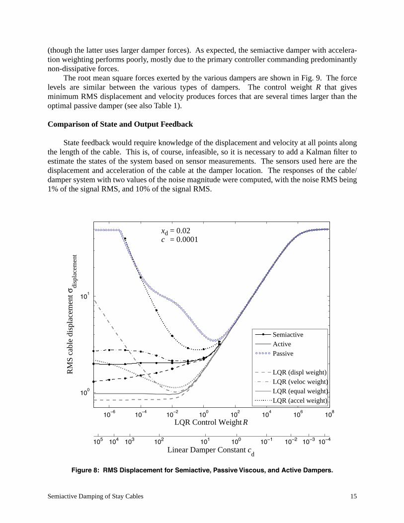
The root mean square forces exerted by the various dampers are shown in Fig. 9. The forcelevels are similar between the various types of dampers. The control weight
R
that givesminimum RMS displacement and velocity produces forces that are several times larger than theoptimal passive damper (see also Table 1).
Comparison of State and Output Feedback
State feedback would require knowledge of the displacement and velocity at all points alongthe length of the cable. This is, of course, infeasible, so it is necessary to add a Kalman filter toestimate the states of the system based on sensor measurements. The sensors used here are thedisplacement and acceleration of the cable at the damper location. The responses of the cable/damper system with two values of the noise magnitude were computed, with the noise RMS being1% of the signal RMS, and 10% of the signal RMS.
Linear Damper Constant cd
105 104 103 102 101 100 10−1 10−2 10−3 10−4
10−6
10−4
10−2
100
102
104
106
108
100
101
LQR Control Weight R
RM
S ca
ble
disp
lace
men
t σdi
spla
cem
ent
SemiactiveActivePassive
LQR (displ weight)LQR (veloc weight)LQR (equal weight)LQR (accel weight)
Figure 8: RMS Displacement for Semiactive, Passive Viscous, and Active Dampers.
x
d = 0.02 c
d = 0.0001
Semiactive Damping of Stay Cables 16
Using the displacement-weighted control (cost in the previous section) of a semiactivedamper, the RMS response using state feedback (LQR) and output feedback (LQG) with bothnoise magnitudes was computed for a range of damper locations. At each damper location, thecontrol weight
R
was chosen so as to minimize RMS cable displacement. Figure 10 shows thatusing output feedback control achieves nearly the same responses as the state feedback controller.
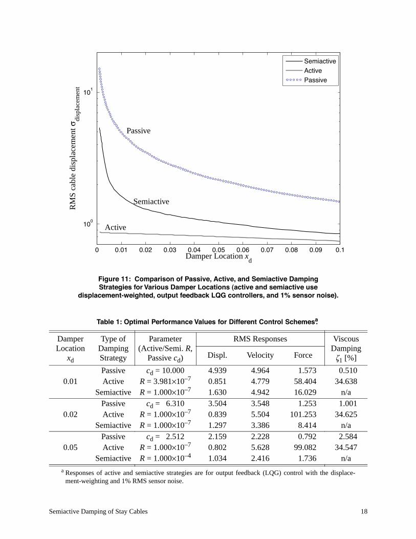
Performance of Damping Strategies over a Range of Damper Locations
The achievable performance of semiactive dampers, in comparison with active and passivedevices, may be seen in Fig. 11 and in Table 1. The active and semiactive strategies here both usethe displacement-weighting controller with output feedback and 1% sensor noise, and the passivedamper is the linear viscous damper giving minimum response for the excitation given above in(24). At each damper location, the displacement-weighted LQG controller that best reduced theRMS displacement is used. (Due to the computational intensity required for finding the controlweight
R
that results in the best semiactive damper performance for a particular damper location,a limited number of values of
R
were used; consequently, the true optimal semiactive perfor-mance may be slightly better (
i.e.
, lower response) than reported here.) For damper locations
Linear Damper Constant cd
105 104 103 102 101 100 10−1 10−2 10−3 10−4
10−6
10−4
10−2
100
102
104
106
108
10−3
10−2
10−1
100
101
LQR Control Weight R
RM
S da
mpe
r fo
rce
σ forc
e
SemiactiveActivePassive
LQR (displ weight)LQR (veloc weight)LQR (equal weight)LQR (accel weight)
Figure 9: RMS Damper Force for Semiactive, Passive Viscous, and Active Dampers.
x
d = 0.02 c
d = 0.0001
J1
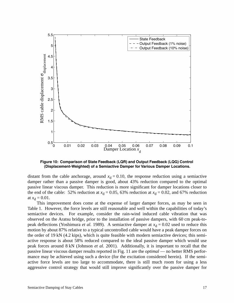
Semiactive Damping of Stay Cables 17
distant from the cable anchorage, around
x
d
= 0.10, the response reduction using a semiactivedamper rather than a passive damper is good, about 43% reduction compared to the optimalpassive linear viscous damper. This reduction is more significant for damper locations closer tothe end of the cable: 52% reduction at
x
d
= 0.05, 63% reduction at
x
d
= 0.02, and 67% reductionat
x
d
= 0.01.This improvement does come at the expense of larger damper forces, as may be seen in
Table 1. However, the force levels are still reasonable and well within the capabilities of today’ssemiactive devices. For example, consider the rain-wind induced cable vibration that wasobserved on the Aratsu bridge, prior to the installation of passive dampers, with 60 cm peak-to-peak deflections (Yoshimura
et al.
1989). A semiactive damper at
x
d
= 0.02 used to reduce thismotion by about 87% relative to a typical uncontrolled cable would have a peak damper forces onthe order of 19 kN (4.2 kips), which is quite feasible with modern semiactive devices; this semi-active response is about 58% reduced compared to the ideal passive damper which would usepeak forces around 8 kN (Johnson
et al.
2001). Additionally, it is important to recall that thepassive linear viscous damper results reported in Fig. 11 are the
optimal
— no better RMS perfor-mance may be achieved using such a device (for the excitation considered herein). If the semi-active force levels are too large to accommodate, there is still much room for using a lessaggressive control strategy that would still improve significantly over the passive damper for
0 0.01 0.02 0.03 0.04 0.05 0.06 0.07 0.08 0.09 0.10.5
1
1.5
2
2.5
3
3.5
4
4.5
5
5.5
Damper Location xd
RM
S ca
ble
disp
lace
men
t σdi
spla
cem
ent
State FeedbackOutput Feedback (1% noise)Output Feedback (10% noise)
Figure 10: Comparison of State Feedback (LQR) and Output Feedback (LQG) Control (Displacement-Weighted) of a Semiactive Damper for Various Damper Locations.
Semiactive Damping of Stay Cables 18
0 0.01 0.02 0.03 0.04 0.05 0.06 0.07 0.08 0.09 0.1
100
101
Damper Location xd
RM
S ca
ble
disp
lace
men
t σdi
spla
cem
ent
SemiactiveActivePassive
Figure 11: Comparison of Passive, Active, and Semiactive DampingStrategies for Various Damper Locations (active and semiactive use
displacement-weighted, output feedback LQG controllers, and 1% sensor noise).
Passive
Semiactive
Active
Table 1: Optimal Performance Values for Different Control Schemesa.
a Responses of active and semiactive strategies are for output feedback (LQG) control with the displace-ment-weighting and 1% RMS sensor noise.
Damper Location
xd
Type of Damping Strategy
Parameter(Active/Semi. R,
Passive cd)
RMS Responses Viscous Damping
ζ1 [%]Displ. Velocity Force
0.01Passive cd = 10.000 4.939 4.964 1.573 0.510Active R = 3.981×10⁻⁷ 0.851 4.779 58.404 34.638
Semiactive R = 1.000×10⁻⁷ 1.630 4.942 16.029 n/a
0.02Passive cd = 6.310 3.504 3.548 1.253 1.001Active R = 1.000×10⁻⁷ 0.839 5.504 101.253 34.625
Semiactive R = 1.000×10⁻⁷ 1.297 3.386 8.414 n/a
0.05Passive cd = 2.512 2.159 2.228 0.792 2.584Active R = 1.000×10⁻⁷ 0.802 5.628 99.082 34.547
Semiactive R = 1.000×10⁻⁴ 1.034 2.416 1.736 n/a
Semiactive Damping of Stay Cables 19
small xd. For example, with a damper location xd = 0.02, the displacement-weighted, output feed-back, semiactive damping strategy that gave the minimum RMS displacement response used acontrol weight R = 10–7, and achieved a 63% decrease in RMS displacement compared to theoptimal passive damper with RMS force 6.7 times that of the passive device. By using a slightlyless aggressive control design, with a control weight R = 10–4, the RMS response is still 57%lower than the optimal passive damper but with a force only 2.5 times that of the passive device;with R = 10–2, the RMS displacement is 50% smaller than that with a passive viscous damper butonly 1.7 times the force.
Table 1 also shows the first-mode viscous damping ratio for the passive and active systemscomputed from the eigenvalues of the closed-loop system. Since the semiactive damper is nonlin-ear, no viscous damping ratio may be computed. However, since the optimal semiactive damperprovides RMS response reduction similar to that of the fully active system, it may be inferred thatan “equivalent” damping ratio on the order of 8% is achievable with a semiactive device.
CONCLUSIONS
The potential of using semiactive dampers to control stay cable vibration has been demon-strated through an analysis of RMS responses and comparison with both passive linear viscousdampers and active dampers with several control designs. The limitations of the response reduc-tions with a passive damper were reviewed. A control-oriented model using an assumed modesmethod with a static deflection shape was developed. This model was shown to be quite accurate,requiring only a few terms for accuracy comparable to that with hundreds of sine-only terms.Consequently, this control-oriented model facilitates low-order control design, evaluation andimplementation. Several families of controllers for the active and semiactive devices weredesigned. Response of the passive and active systems were computed exactly via a Lyapunovequation, whereas semiactive system responses were computed using simulation.
A semiactive damper located 2% of the distance from the end of the cable, using a clippedoptimal control algorithm with output feedback, weighting cable RMS displacement, was seen todecrease RMS responses to 63% lower than that of an optimal viscous damper, nearly the 76%achieved by fully active devices. Similar improvements may be observed at other damper loca-tions. The equivalent modal damping of the first mode with a semiactive damper is significantlyhigher — about 8% of critical — than the optimal passive device, which can only add 1%damping for a damper location at xd = 0.02. Thus, semiactive dampers have the potential toprovide significantly improved mitigation of stay cable vibration.
There are several additional issues, such as the complexity of the cable model, not discussedherein that have been studied elsewhere. While the level of sag in cables of cable-stayed bridgesis typically small (Irvine 1981), passive damper performance is reduced some by cable sag (e.g.,Sulekh 1990; Xu and Yu 1998; Krenk and Nielsen 2002); a study by the authors of the perfor-mance of semiactive damping for inclined flat-sag cables with axial flexibility is reported inJohnson et al. (2003). Additionally, Irvine (1981) also indicates that the flexural rigidity presentin most cables is small, but cable bending stiffness is known to decrease the performance of theoptimal passive damper; while this has not been extensively studied for semiactive control, theperformance of active control was shown in Christenson (2001) to be relatively unaffected bycable flexural rigidity. Christenson (2001) also investigates more realistic models of semiactivedampers, such as magnetorheological fluid dampers, for cable vibration mitigation. Finally, a lab-
Semiactive Damping of Stay Cables 20
oratory experiment is discussed in Christenson (2001) and Christenson et al. (2006), and full-scale applications in Duan et al. (2005).
ACKNOWLEDGMENTS
The authors gratefully acknowledge the partial support of this research by the NationalScience Foundation, under grants CMS 95-00301, CMS 95-28083 and CMS 99-00234 (Dr. S.C.Liu, Program Director), and the LORD Corporation.
The genesis of this work occurred while Prof. Fujino was the visiting Melchor Chaired Pro-fessor of Civil Engineering at the University of Notre Dame, Fall 1997, and while Prof. Johnsonwas a Visiting Research Assistant Professor of Civil Engineering at the University of Notre Dame,Fall 1997 – Summer 1999.
APPENDIX I. REFERENCES
Craig, R., Jr. (1981). Structural Dynamics: An Introduction to Computer Methods, John Wiley & Sons, New York,350–353.
Christenson, R.E. (2001). “Semiactive Control of Civil Structures for Natural Hazard Mitigation: Analytical andExperimental Studies.” Ph.D. dissertation, University of Notre Dame, Notre Dame, Indiana.
Christenson, R.E., Spencer, B.F., Jr., and Johnson, E.A. (2006). “Experimental Verification of Smart CableDamping.” Journal of Engineering Mechanics, ASCE, 132(3), 268–278.
Duan, Y.F., Ni, Y.Q., and Ko, J.M. (2005). “State-Derivative Feedback Control of Cable Vibration using SemiactiveMagnetorheological Dampers.” Computer-Aided Civil and Infrastructure Engineering, 20(6), 431–449.
Dyke, S.J., Spencer, B.F., Jr., Sain, M.K., and Carlson, J.D. (1996a). “Seismic Response Reduction Using Magne-torheological Dampers.” Proc. IFAC World Congress, San Francisco, CA, Vol. L, 145–150.
Dyke, S.J., Spencer, B.F., Jr., Sain, M.K., and Carlson, J.D. (1996b). “Modeling and Control of MagnetorheologicalDampers for Seismic Response Reduction.” Smart Materials and Struct., 5(5), 565–575.
Endo, T., Iijima, T., Okukawa, A., and Ito, M. (1991). “The Technical Challenge of a Long Cable-Stayed Bridge —Tatara Bridge”. In M. Ito, Y. Fujino, T. Miyata, and N. Narita (eds.), Cable-stayed Bridges — Recent Develop-ments and their Future, Elsevier, 417–436.
Fujino, Y., Soong, T.T., and Spencer, B.F., Jr. (1996). “Structural Control: Basic Concepts and Applications.”Proceedings of the ASCE Structures Congress XIV, Chicago, Illinois, April 15–18, 1996, 1277–1287.
Fujino, Y., Warnitchai, P., and Pacheco, B.M. (1993). “Active Stiffness Control of Cable Vibration.” Journal ofApplied Mechanics, ASME, 60(4), 948–953.
Gimsing, N.J. (1983). Cable-Supported Bridges, John Wiley & Sons, Chichester, England.Hikami, Y. (1986). “Rain Vibrations of Cables of Cable Stayed Bridge.” Journal of Wind Engineering, JAWE, no. 27,
17–28 (in Japanese).Hikami, Y. and Shiraishi, N. (1988). “Rain-Induced Vibrations of Cables in Cable-Stayed Bridges.” Journal of Wind
Engineering and Industrial Aerodynamics, 29(1–3), 409–418.Housner, G.W., Bergman, L.A., Caughey, T.K., Chassiakos, A.G., Claus, R.O., Masri, S.F., Skelton, R.E.,
Soong, T.T., Spencer, B.F., Jr., and Yao, J.T.P. (1997). “Structural Control: Past and Present.” Journal of Engi-neering Mechanics, ASCE, 123(9), 897–971.
Irvine, H.M. (1981). Cable Structures, MIT Press, Cambridge, Massachusetts.Johnson, E.A., Ramallo, J.C., Spencer, B.F., Jr., and Sain, M.K. (1999a). “Intelligent Base Isolation Systems.” Proc.
Second World Conf. on Struct. Control, Kyoto, Japan, Vol.1, 367–376. Johnson, E.A., Baker, G.A., Spencer, B.F., Jr., and Fujino, Y. (2001). “Semiactive Damping of Stay Cables
Neglecting Sag.” Technical Report No. USC-CE-01-EAJ1, Dept. of Civil and Environmental Engineering,University of Southern California. Available online at http://rcf.usc.edu/~johnsone/papers/smartdamping_tautcable_rpt.html
Semiactive Damping of Stay Cables 21
Johnson, E.A., Christenson, R.E., and Spencer, B.F., Jr. (2003). “Semiactive Damping of Cables with Sag.”Computer Aided Civil and Infrastructure Engineering, 18(2), 132–146.
Johnson, E.A., Spencer, B.F., Jr., and Fujino, Y. (1999b). “Semiactive Damping of Stay Cables: A PreliminaryStudy.” Proceedings of the 17th International Modal Analysis Conference (IMAC XVII), Society for ExperimentalMechanics, Bethel, Connecticut, 417–423.
Kovacs, I. (1982). “Zur Frage der Seilschwingungen und der Seildämpfung.” Die Bautechnik, 59(10), 325–332, (inGerman).
Krenk, S. (2000). “Vibrations of a Taut Cable with an External Damper.” Journal of Applied Mechanics, ASME,67(4), 772–776.
Krenk, S., and Nielsen, S.R.K. (2002). “Vibrations of a Shallow Cable with a Viscous Damper.” Proceedings of theRoyal Society of London, Ser. A, 458(2018), 339–357.
Krenk, S., and Høgsberg, J.R. (2005). “Damping of Cables by a Transverse Force.” Journal of EngineeringMechanics, ASCE, 131(4), 340–348.
Main, J.A. and Jones, N.P. (1999). “Full-Scale Measurements of Stay Cable Vibration.” In A. Larsen, G.L. Laroseand F.M. Livesey (eds.), Wind Engineering into the 21st Century, Balkema, Rotterdam, 963–970.
Main, J.A., and Jones, N.P. (2002a). “Free Vibrations of Taut Cable with Attached Damper. I: Linear ViscousDamper.” Journal of Engineering Mechanics, ASCE, 128(10), 1062–1071.
Main, J.A., and Jones, N.P. (2002b). “Free Vibrations of Taut Cable with Attached Damper. II: Nonlinear Damper.”Journal of Engineering Mechanics, ASCE, 128(10), 1072–1081.
Matsumoto, M. (1998). “Observed Behavior of Prototype Cable Vibration and its Generation Mechanism.” In A.Larsen and S. Esdahl, eds., Bridge Aerodynamics, Balkema, Rotterdam, 189–211.
Pacheco, B.M., Fujino, Y., and Sulekh, A. (1993). “Estimation Curve for Modal Damping in Stay Cables with ViscousDamper.” Journal of Structural Engineering, ASCE, 119(6), 1961–1979.
Poston, R.W. (1998). “Cable-Stay Conundrum.” Civil Engineering, 68(8), 58–61.Russell, H. (1999). “Hong Kong Bids for Cable-Stayed Bridge Record.” Bridge Design and Engineering, No. 15
(second quarter), 7.Scanlon, R.H. (1999). Personal communication with Erik A. Johnson, February 22, 1999.Spencer, B.F., Jr., Dyke, S.J., Sain, M.K., and Carlson, J.D. (1997). “Phenomenological Model for Magnetorheolog-
ical Dampers.” ASCE Journal of Engineering Mechanics, 123(3), 230–238.Spencer, B.F., Jr. and Sain, M.K. (1997). “Controlling Buildings: A New Frontier in Feedback.” IEEE Control
Systems Magazine, 17(6), 19–35. Stengel, R.F. (1986). Stochastic Optimal Control: Theory and Application, John Wiley & Sons, New York.Sulekh, A. (1990). Non-dimensionalized Curves for Modal Damping in Stay Cables with Viscous Dampers, Master’s
Thesis, Department of Civil Engineering, University of Tokyo, Tokyo, Japan.Virloguex, M., et al. (1994). “Design of the Normandie Bridge”. Proceedings of the International Conference on
Cable-Stayed and Suspension Bridges, IABSE, Deauville, France, Vol. 1, 605–630.Watson, S.C. and Stafford, D. (1988). “Cables in Trouble.” Civil Engineering, ASCE, 58(4), 38–41.Xu, Y.L., and Yu, Z. (1998). “Vibration of Inclined Sag Cables with Oil Dampers in Cable-Stayed Bridges.” Journal
of Bridge Engineering, 3(4), 194–203.Yamaguchi, H. and Dung, N.N. (1992). “Active Wave Control of Sagged-Cable Vibration.” Proceedings of the First
International Conference on Motion Vibration Control, Yokohama, Japan, 134–139.Yamaguchi, H. and Fujino, Y. (1998). “Stayed Cable Dynamics and its Vibration Control.” In A. Larsen and S.
Esdahl, eds., Bridge Aerodynamics, Balkema, Rotterdam, 235–253.Yang, G., Spencer, B.F., Jr., Carlson, J.D., and Sain, M. K. (2002). “Large-scale MR Fluid Dampers: Modeling and
Dynamic Performance Considerations.” Engineering Structures, 24(3), 309–323.Yoshimura, T., Inoue, A., Kaji, K., and Savage, M. (1989). “A Study on the Aerodynamic Stability of the Aratsu
Bridge.” Proceedings of the Canada-Japan Workshop on Bridge Aerodynamics, Ottawa, Canada, 41–50.
APPENDIX II. NOTATION
The following symbols are used in this paper:
Semiactive Damping of Stay Cables 22
, partial derivatives with respect to and
dimensional quantity
eigenfunction L2 norm
, , matrices in state equation
, , estimator state equation matrices
cable damping per unit length
viscous damping coefficient of attached passive linear viscous damper
, , matrices in regulated outputs equation
, , matrices in sensor equation
, modified state and output matrices for passive damper
expectation operator
force commanded by primary controller
, external load coefficient on ith generalized displacement, external load vector
external distributed load on the cable
kth cost function
, , cable length, tension, mass per unit length (dimensional)
state feedback gain for the kth cost function
Kalman filter estimator gain
, , mass, damping, and stiffness matrices
number of shape functions used in expansion of
, , elements of mass, damping, and stiffness matrices
solution to estimator algebraic Riccati equation
solution to control design algebraic Riccati equation
weight on output for the kth cost function
, covariance (or spectral density magnitude) of excitation and sensor noise
, ith generalized displacement and generalized displacement vector
control weight in cost function
excitation spectral density magnitude matrix
sensor noise vector
transverse deflection of the cable
, displacement and acceleration at the damper location
, velocity at the damper location
zero-mean Gaussian white noise excitation process
, damper location and its force
vector of noisy sensor measurements
( )′ ̇( ) x t
·( )· 2
A B G
AKF BKF GKF
c
cd
Cz Dz Hz
Cy Dy Hy
AP CP
E ·[ ]Fd
active t( )
fi f
f x t,( )
Jk
L T ρ
Lk
LKF
M C K
m v x t,( )
mij cij kij
P̃
Pk
Qk
QKF RKF
qi t( ) q t( )
R
S0
v
v x t,( )
v xd t,( ) v̇̇ xd t,( )
v̇ xd t,( ) v̇d
W t( )
xd Fd t( )
y
Semiactive Damping of Stay Cables 23
vector of generalized coordinates and their derivatives
, variables used in expansion of external distributed load
force modulation function
Dirac delta function
Kronecker delta
state vector
estimate of the state vector
the solution to a Lyapunov equation
RMS cable acceleration
RMS cable displacement
RMS cable velocity
, ith shape function and shape function vector
ith mode computed using shape functions
ith mode computed using 499 sine shapes plus the static deflection shape
, damper load coefficient on ith generalized displacement, damper load vector
fundamental natural frequency of the undamped cable
ωi, ζi, natural frequency, damping ratio, and eigenfunction of the ith mode
z qT q̇T q̇̇˜
T[ ]T
αi x( ) ββββ t( )
α v̇( )
δ ·( )
δij
ηηηη qT q̇T[ ]T
ηηηη̂ ηηηηΣΣΣΣσacceleration
σdisplacement
σvelocity
φi x( ) φφφφ x( )
φ̃im x( ) m
φ̃i499s sd+ x( )
ϕi ϕϕϕϕ
ω0
φ̃i x( )