Western Region

SALT LAKE CITY,

UTAH

July, 1970

ESSA WBTM. WR 52

ESSA Technical Memorandum WBTM WR 52 U.S. DEPARTMENT OF COMMERCE ENVIRONMENTAL SCIENCE SERVICES ADMINISTRATibN

Weather Bureau

Sacramento Weather Radar Climatology

R. G. PAPPAS AND C. M. VELIQUETTE

WESTERN· REGION TECHNICAL MEMORANDA

The Technical Memoranda series provide an informal medium for the documentation and quick dis­semination of results not appropriate, or not yet ready, for formal publication in the standard journals. The series are used to report on work in progress, to describe technical procedures and practices, or to report to a limited audience. These Technical Memoranda will report on investigations devoted primarily to Regional and local problems of interest mainly to Western Region personnel, and hence will not be widely distributed.

These Memoranda are available from the Western Region Headquarters at the following address: Weather Bureau Western Region Headquarters, Attention SSD, P. 0. Box 11188, Federal Building, Salt Lake City, Utah 84111.

The Western Region subseries of ESSA Technical Memoranda, No. 5 (revised edition), No. 10 and all others beginning with No. 24, are available also from the Clearinghouse for Federal Scien­tific and Technical Information, U. S. Department of Commerce, Sills Building, Port Royal Road, Springfield, Va. 22151. Price: $3.00 paper copy; $0.65 microfiche. Order by accession number shown in parentheses at end of each entry.

Western Region Technical Memoranda:

No. 1* No. 2

No. 3 No. 4 No. 5**

No. 6 No. 7 No. 8 No. 9 No. 10* No. 11 No. 12*

No. 13

No. 14

No. 15

No. 16 No. 17

No. 18 No. 19

No. 20

No. 21

No. 22 No. 23

No, 24

No. 25

No. 26

Some Notes on Probability Forecasting. Edward D. Diemer. September 1965. Climatological Precipitation Probabilities. Compiled by Lucianne Miller.

December 1965. Western Region Pre- and Post-FP-3 Program. Edward D. Diemer. March 1966. Use of Meteorological Satellite Data. March 1966. Station Descriptions of Local Effects on Synoptic Weather Patterns. Philip Williams.

October 1969 (Revised). (PB-178 000) Improvement of Forecast Wording and.Format. C. L. Glenn. May 1966. Final Report on Precipitation Probability Test Program. Edward D. Diemer. May 1966. Interpreting the RAREP. Herbert P. Benner. May 1966. (Revised January 1967.) A Collection of Papers Related to the 1966 NMC Primitive-Equation Model. June 1966. Sonic Boom. Loren Crow (6th Weather Wing, USAF, Pamphlet). June 1966. (AD-479 366) Some Electrical Processes in the Atmosphere. J, Latham. June 1966. A Comparison of Fog Incidence at Missoula, Montana, with Surrounding Locations.

Richard A. Dightman. August 1966. A Collection of Technical Attachments on the 1966 NMC Primitive-Equation Model.

Leonard W. Snellman. August 1966. Applications of Net Radiometer Measurements to Short-Range Fog and Stratus Forecast­

ing at Los Angeles. Frederick Thomas. September 1966. The Use of the Mean as an Estimate of "Normal" Precipitation in an Arid Region.

Paul c. Kangieser. November 1966. Some Notes on Acclimatization in Man. Edited by Leonard w. Snellman. November 1966. A Digitalized Summary of Radar Echoes Within lOC Miles of Sacramento, California.

J, A. Youngberg and L. B. Overaas. December 1966. Limitations of Selected Meteorological Data. December 1966. A Grid Method for Estimating Precipitation Amounts by Using the WSR-57 Radar.

R. Granger. December 1966. Transmitting Radar Echo Locations to Local Fire Control Agencies for Lightning Fire

Detection. Robert R. Peterson. March 1967. An Objective Aid for Forecasting the End of East Winds in the Columbia Gorge. D. John

Coparanis. April 1967. Derivation of Radar Horizons in Mountainous Terrain. Roger G. Pappas. April 1967. "K" Chart Application to Thunderstorm Forecasts Over the Western United States,

Richard E. Hambidge. May 1967.

Historical and Climatological Study of Grinnell Glacier, Montana. Richard A. Dightman. July 1967. (PB-178 071)

Verification of Operational Probability of Precipitation Forecasts, April 1966 -March 1967. W. W. Dickey. October 1967. (PB-176 240)

A Study of Winds in the Lake Mead Recreation Area. R. P. Augulis. January 1968. (PB-177 830)

IIIQut of Print **Revised

A western Indian symbol for rain. It also symbolizes man's dependence on weather and environment in the .West.

I ·i

WESTERN REGION

U. S. DEPARTMENT OF COMMERCE ENVIRONMENTAL SCIENCE SERVICES ADMINISTRATION

WEATHER BUREAU

Weather Bureau Technical Memorandum WR-52

SACRAMENTO WEATHER RADAR CLIMATOLOGY

R. G •. Pappas Weather Bureau Office Sacramento, California

C. M. Veliquette Weather Bur.eau Office Sacramento, California

TECHNICAL MEMORANDUM NO. 52

SALT LAKE CITY, UTAH JULY 1970

TABLE OF CONTENTS

List of Figures iii

Abstract

I. Introduction

II. Data 2

I II. Limitations 2-4

IV. Annua I, Seasonal, and Monthly Echo Frequency Distributions 5-6

v. Conclusions 6-7

VI. References 7

i i.

Figure I (a)

Figure I (b)

Figure 2

Figure 3

Figure 4

Figure 5

Figure 6

Figure 7

Figure 8

Figure 9

Figure 10

Figure II

Figure 12

Figure 13

Figure 14

Figure 15

Figure 16

Figure 17

Figure 18

Figure 19

Figure 20

Figure 21

Table I

LIST OF FIGURES AND TABLE

Example of Radar Climatology Computer Output in Map Format

Example of Radar Climatology Computer Output in Map Format

Average Annual Precipitation (Inches) Map Deter­mined from Radar Integer Data

Average Annual Gauge Precipitation During Period of Radar Record

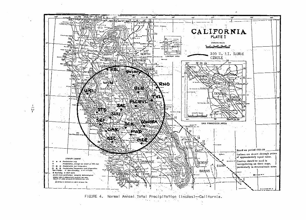
Normal Annual Total Precipitation (lnches)-­Ca I i torn i a

Average Annual Hourly Echo Frequencies

Average "Wet" Season <October-Apr i I ) Hour I y Echo Frequencies

Average "Wet" Season Gauge Precipitation During Period of Radar Record

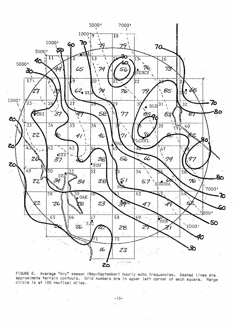
Average "Dry" Season (May-September) Hourly Echo Frequencies

Average "Dry" Season Gauge Precipitation During Period of Radar Record

Average January Hourly Echo Frequencies

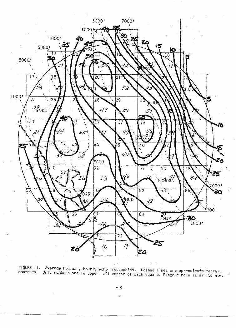
Average February Hourly Echo Frequencies

Average March Hourly Echo Frequencies

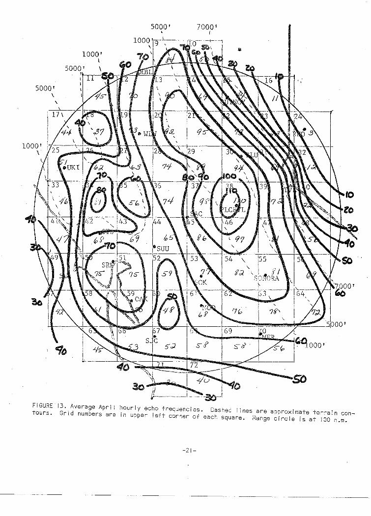
Average Apri I Hourly Echo Frequencies

Average May Hourly Echo Frequencies

Average June Hourly Echo Frequencies

Average July Hourly Echo Frequencies

Average August Hourly Echo Frequencies

Average September Hourly Echo Frequencies

Average October Hourly Echo Frequencies

Average November Hourly Echo Frequencies

Average December Hourly Echo Frequencies

Precipitation Stations

iii

8

9

10

II

12

13

15

16

17

18

19

20

21

22

23

24

25

26

27

28

29

4

SACRAMENTO WEATHER RADAR CLIMATOLOGY

ABSTRACT

A climatology of weather radar echoes within 100 nautical miles (n.m.) of Sacramento, California is derived by transferring hourly overlay data onto a coarse grid system. While the program is capable of summarizing rainfal I intensities and amounts, I imitations in reflecti­vity--rainfal I intensity relationships, particularly for the precipita­tion climatology of the Sacramento coverage area, severely restrict the uti I ity of such data. However, occurrences of weather echoes, without regard to intensity, do correlate wei I with normal and observed areal precipitation patterns. The relatively short period of record precludes application of the data in a true climatological sense.

I. INTRODUCTION

An earlier report by Youngberg and Overaas (1966) presented a detailed account of the Sacramento radar climatology program. The Sacramento study and others (e.g., Parrish and Lopez, 1968, or Landers, 1969) have usually summarized only a smal I amount of data and were aimed primarily at describing techniques and capabi I ities of the program. Subsequent to the earlier Sacramento report, the avai !able data bank has grown to about seven years of hourly radar data in digitized form, probably one of the longest periods of record for this type of data. Approximately six years (74 months) of the data have now been tabulated, beginning with July 1962 and extending through December 1968, except for the period September-December 1964, when the radar was being moved. Data tor 1969 has not yet been processed. A total of 74 months was used in the tabulation.

II. DATA

The earlier work by Youngberg and Overaas (1966) presented a complete explanation of the data base and technique used. In brief: the data base consists of hourly radar overlays which are traced from the Sacramento WSR-57 PPI scope. These overlays include contours of echo intensity in the operational c~tegories specified in the Weather Radar Manual (1967). They a·re'dstehn·ined frbrh a sHmdard rainfall intensity-­reflectivity relationship, Ze = 200rl.6, where Ze is reflectivity in mm6/m3 and I is rainfal I in mm/hr. The various intensity levels, very weak, weak, moderate, strong, and very strong, are color coded on the overlay for ease of interpretatfon~--This overlay is an operational too I l n the Sacramento .rad:CJr :prograll), b~t a IS() serves: as{ an. i nva I uab I e radar data source,,: inc Lud i.ng its us.e i.n the, c l;i rna.tq logy study. I nfe.n­siti'es 'wi,thin appro~irnc:~tely 100 ,n.m. o(:t8e.radar qre digiti.zed b'0 p lac i,ng. a grLpqed te~p.l a_te .qv(3r:: thE) over l,ay. and coding the lntens;ity tor. ea~h ~rid' sqL(a,re

1qnfo -~ ... Pu,nch,qard. ::he gr;~d ,Js ;coa)r.se., 64 squares

each 22!15 by 2?.15 .n.ty~ .. ,, but allow? al.l. lntens.1:ty da.ta ,from :an overlay to}e punc~E:ld on one s:ar:d. The gridde.d t.empi.;;Jte,c:onsists of cutout "wi ndow~", a~outone;n i nth th_e -a re?l of. the square.s.; in · . .thel ~s.nter of ·e.ach gr;id sq~Jare, a:n9.,.the high(:l,st int131:1sity. ob..serve:d ,in the "window'' 'i's the 'intensity_ E?~.GodeQ •. .--::·:·, ·: · ! ~~ •. · I.

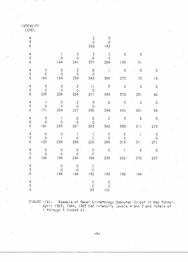
The data may then be computer processed in a variety of ways, the most common uti I izing a program th~t: prints .. ;1-he,. hourly frequency of each integer in a map format for any time period desired--day, storm, month, etc. F.]gu.t;'~S I Ca -~ and 11( b) are ,a su,mm,ar,y. of :Ap rJ I data for ·three : · years and al.so an,e>xample pf the, map forrn.at .. The l0cw.est three, i.ntensity jnte'gers, I, 2,_and'j, are SUmriJE;ld for each·,gl7id,sqwar.e·ir:J Fi.gur,e:.l,(a.); whiie .. Jhtegers 4'and .~.and th~ tq;tals of. l,:t.hrough 5 (toded .6). are. in Figure. l(b) •.. · · · · · .. · ...

. ' ' '···' II I .

I

LIMITATIONS , : . • • 1 , , • ~ • · r J ·! r ' \.'

Lfrnl'ts tnorerestrlcfiye tha~ those us~a.lly plac<i~Jd on the reiJabllity.,of radar d~ta (Baftan~ 1~59.; Hiser and Fry~.emc;~n,,19,59;. WlJsc::>n, ·1964).:mu~t b'e app I 'i ed to the SacrCJmento radar dat~, (,V'{F?a:v,e,r ,

1 I 966 ).. , AI though the

antenna is located 'on top of a tal I building, moderately,·high terraith in the Coast Ranges to the west and high ranges of the Sierra Nevada to the east causes severe blocking over much of the coverage area, in addition to the usual range I imitations caused by beam divergence and earth's curvature (Pappas, 1967, 1969). Complete overshooting of pre­cipitation echoes results mostly at ranges more distant than those used in this radar climatology project (i.e., beyond 100 n.m.), but partic;~l

blocking combined with strong low level orographic effects causes sig­nificant underestimation of intensities during the "wet" season (Pappas, 1969). Convective thunderstorm activity, which occurs almost entirely over the higher ranges of the Sierra Nevc;~da and in Nevada in summer, is detected much more readily due to the high tops attained by these echoes.

-2-

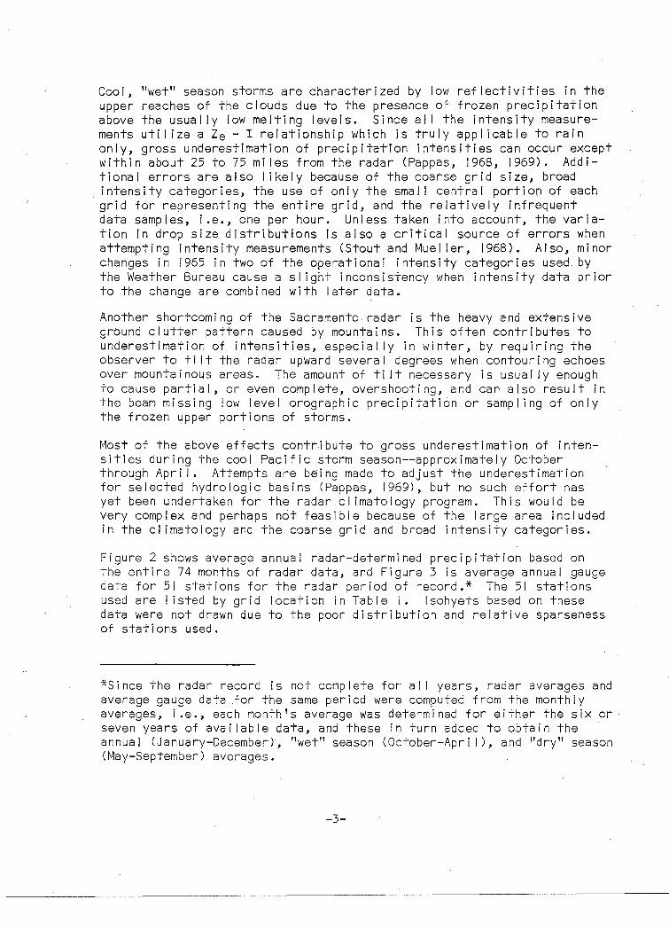
Cool, "wet" season storms are characterized by low reflectivities in the upper reaches of the clouds due to the presence of frozen precipitation above the usually low melting levels. Since alI the intensity measure­ments uti I ize a Ze- I relationship which is truly appl !cable to rain only, gross underestimation of precipitation intensities can occur except within about 25 to 75 miles from the radar (Pappas, 1968, 1969). Addi­tional errors are also I ikely because of the coarse grid size, broad intensity categories, the use of only the smal I central portion of each grid for representing the entire grid, and the relatively infrequent data samples, i.e., one per hour. Unless taken into account, the varia­tion in drop size distributions is also a critical source of errors when. attempting intensity measurements (Stout and Mueller, 1968). Also, minor changes in 1965 in two of the operational intensity categories used by the Weather Bureau cause a slight inconsistency when intensity data prior to the change are combined with later data.

Another shortcoming of the Sacramento radar is the heavy and extensive ground clutter pattern caused by mountains. This often contributes to underestimation of intensities, especially in winter, by requiring the observer to ti It the radar upward several degrees when contouring echoes over mountainous areas. The amount of ti It necessary is usually enough to cause partial, or even complete, overshooting, and can also result in the beam missing low level orographic precipitati6n or sampling of only the frozen upper portions of storms.

Most of the above effects contribute to gross underestimation of inten­sities during the cool Pacific storm season--approximately October through Apri I, Attempts are being made to adjust the underestimation for selected hydrologic basins (Pappas, 1969), but no such effort has yet been undertaken for the radar climatology program. This would be very complex and perhaps not feasible because of the large area included in the climatology and the coarse grid and broad intensity categories.

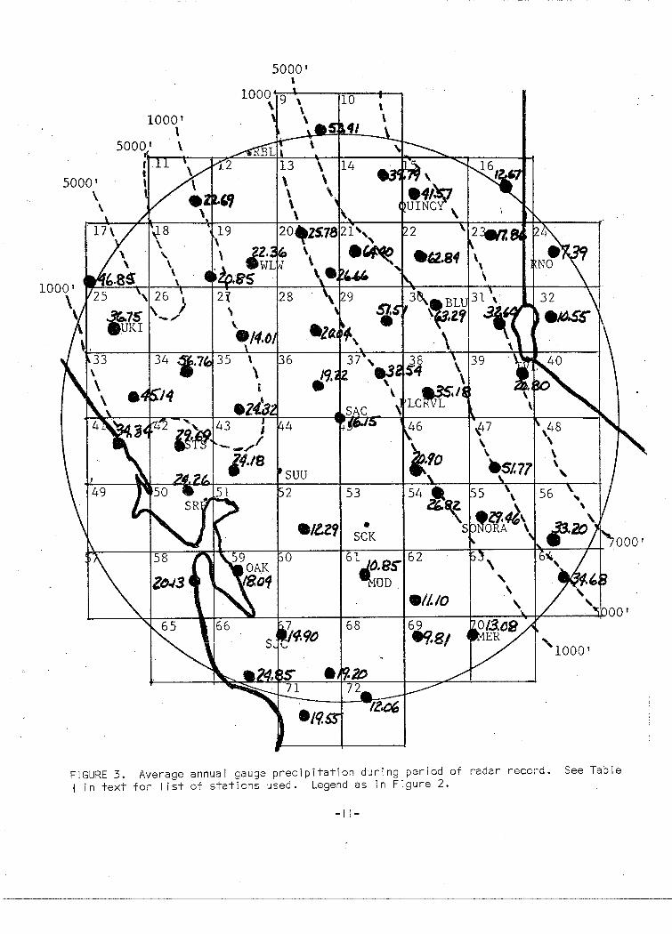
Figure 2 shows average annual radar-determined precipitation based on the entire 74 months of radar data, and Figure 3 is average annual gauge data for 51 stations for the radar period of record.* The 51 stations used are I isted by grid location in Table I. lsohyets based on these data were not drawn due to the poor distribution and relative sparseness of stations used.

*Since the radar record is not complete for alI years, radar averages and average gauge data for the same period were computed from the monthly averages, i.e., each month's average was determined for either the six or seven years of available data, and these in turn added to obtain the · annua I (January-December), "wet" season COctober-Apri I), and "dry" season (May-September) averages.

-3-

:

T~SLE I

PRECIPfTATibN STATlONS

GRID GRlD GRID NO .• ' STATION' No: '':'

STATION STATtON NO. , . ,

: ;-.. .. 9 Mineral 29

•' Grass Valley 50 Peta I t.lma

'II Pe~skenta 30 Blue Canyon 52 Antioch .14 '8reenvi lie: 31 Tahoe ~ity 54 San Andreas 15: :ouincy 32 ·carson City % Sonora . ,

.Doyle Cloverdale· 56 Hefch Hetchy 16 3_3 17· ' .. Wi I lets 34 Hobergs 58 San Francisco 18 Stc;>nyford 35 Lake Berryessa 59 Oak I and

'19 Wi I lows 36 Nicolaus 61 Modesto 20 Orovi II e '31 Auburn 62 Turlock 20 Chico 38 PI acervi I I e 64 Yosemite 2r . .BrLJsh Cre.ek 39 Wood fords 66 Davenport '\!

22 Downievi I le 41. Fort Ros~ 67 ,San Jose 2.3 Loyalton 42 Santa Rosa 67 Gi I roy

. 24' Reno 43 Napa 69 ,Newman 25 Ukiah 44 Sacramento 70 Merced 27 Wi I I lams 46 ·lone 71 Wc;Jtsonv i I I e 28 Yuba City 47 Calaveras R~S. 72 · Ho IIi ster

Ex2ep:t for:. grids' immed'iately adjacent to Sacra~en,to, which ?.lre remar,kably near both clih)atol\).gical normals(Figure-4) and average a,nnual precip:ita­tloni (Figure 3), radar determined precipitation in Figl.!re 2 appe,ars to Under:esfi.mate by -~ factor fan_g in'g. f,,rom l.ess than t,WO: to as much as fifteen. l,r) .Figure" 2, th!'l fact that the northernmost grid~ iare indicated to have tonsideral:>ly more precipitation than those furthest southis realistic, but amounts a·re still gross underestimates. The overall radar-determined pre~ipitation distribution is one of decreasing amoun'ts with distance· in all directions from Sacramento, which is, of course, true only to the southeast e>ver the· Saq Joaquin Va '11 ey, and to the northwest over the I ower Sai:::r?.lmehto 'y~ i. I ey.. . , ,

A ltholigh not shown here, the sam~ deficiency is demons.trated in tabu I at ions of the frequency of each integer for the "wet" season. These tabulations show the heavier integers (3, 4, and 5) occurring almost exclusively in the grids nearest to Sacramento. Contributing to this, and also very I i~ely c~~sing some,overestimation of intensitfes.near the radar, is· the effect of the rada'r beam samp I i ng the me It i ng I ayer or bright band at close ranges (Weather Rada~ Manual, 1967). A~ would be ~~pected for rea­s6hs ~iven above, no such. deficiency is indicated for the~ summer convec-tive ~~asoh. ·

Limitations due to the short period of record are significant, particularly for so highly variable a parameter as precipitation. Therefore, appl !ca­tions of the technique must be made with caution and conclusions reached considered as only tentative.

-4-

IV. ANNUAL, SEASONAL, AND MONTHLY ECHO FREQUENCY DISTRIBUTIONS

The tabulation of average annual echo frequency for each grid square, without regard to intensities, for alI 74 months of data is presented in Figure 5. The 500-echo frequency isopleth in the Coast Range and the 600 isopleth in the Sierra Nevada correspond fairly wei I with areas of maximum normal (Figure 4) and sample period average (figure 3) pre­cipitation, with orographic effects playing a major role in the distri­bution. However, the primary maximum, shown by the 650 isopleth, is shifted southward from its normal or sample period position. This is probably due mostly to the ranging I imitations discussed in Section I I I. The overal I decrease in frequencies from north to south is realistic; however, some of the rapid decrease near grid edges is due to range and blocking I imitations.

Figure 6 is the echo frequency tabulation for the lfwetlf season months, October through Apri I. Again, a slight southward shift of the Sierra Nevada maximum is indicated if compared with the averages in Figure 7. The maximum in the Coast Range at grid 34 also corresponds with maximum in Figure 7. However, high values shown in grids 33 and 17 of Figure 7 are not indicated in the radar analysis, Figure 6, probably due to range I imitations. The rapid decrease in echo frequencies in the lee of the Sierra is due most I y to the norma I I ee rain-shadow effect and agrees we I I with the gauge averages (Figures 4 and 7). This decrease also results to some degree from range I imitations and blocking.

I!Drylf season (May through September) totals are presented in Figure 8. In this case, echo maximum areas enclosed by the 90 isopleths are in two different portions of the Sierra Nevada. These compare favorably with gauge averages in Figure 9, which indicate maxima in grtds 30 and 56 (unfortunately, no gauge data were computed for grid. 4~). The minimum in the northern Sierra at grid 14 (60 isopleth in Figure 8) reflects a minimum gauge precipitation area in the same grid in Figure 9. More about the "dry" season distributions wi II be included in the discussion of monthly averages.

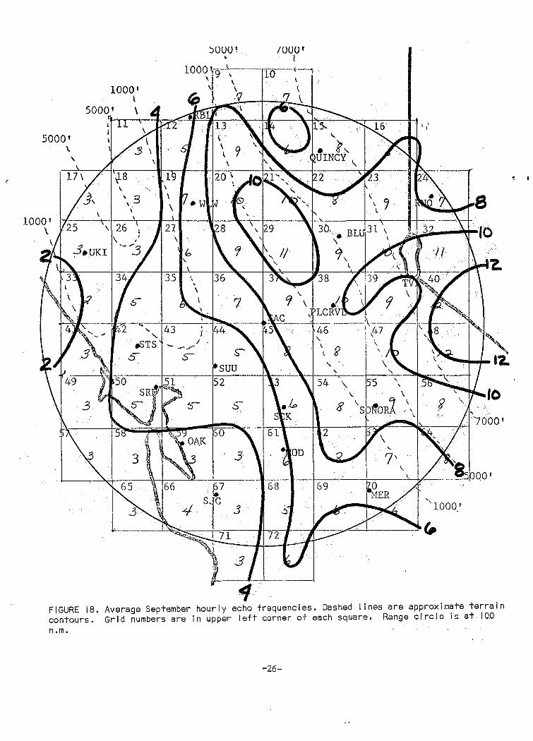
Monthly frequency averages are presented in Figures 10 through 21. Generally, the rapid decrease in echo frequency between the "wet" and "dry" seasons is indicated by comparing Apri I (Figure 13) and May (Figure 14). The reverse transition from October (Figure 19) to November (figure 20) is also very pronounced.

Beginning in May, an eastward to southeastward shift in echo frequency maximum occurs. In May, the evidence is only a submaximum (30 isopleth) in grid 48. By July the maximum has shifted east of the Sierra Nevada crest and continues there through September. This shift is attributed to the waning influence of westerly disturbances during summer months and the increasing effect of moist unstable air masses penetrating the coverage area from the southeast, with orographic I ifting and surface heating helping to trigger further instabi I ity. Additionally, nondetec­tion of much of the distant cool, "wet" season precipitation contrasted with enhanced summertime detection capabi I ity, as discussed in section

-5-

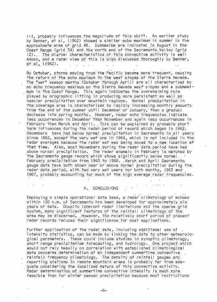
Ill, probably influences t_hli3 magnitude of t~is shift. An earlier study by Benrier, et al, (1962) showed a similar echo maximum i~ summer in the approxi.mat·e area of, gr iq 48. Submax i ma .are indIcated in August in the Coast Range (grid34) and the north end of the Sacrament9Valley (gri.d 12) .. ·The diurnal characteristics of. this convE;Jctive activity is. well kriown, and a radar view of this is al£;6 discussed thoroughly by Benner, et a I '· ( I 962) • ·

By October, storms moving from the Pacific become more frequent~ causing the r.eturn of the echo m<:lx i mum to the west s I opes of the Sierra Nevada. The ''wet" season months (October t,hrough Apri I) are a II character I ;zed by an echo frequency maximum on the Sierra NE;Jvada west· slopes and a submaxi­

.mum in fhe Coast Range. This again indicates the overwhelming role ~layed by orographic lifting in producing more persistent as wei I ~s heavier precipitation over mountain regions. Normal precipitation in thecoverage area is characterized by rapidly increasing monthly f.Jmounts 'from the end of the summer unti I December or January, then a gradua I decrease intospring months. However, radar echo frequencies indicate I ess occurrences In Qecember. than November and agaIn I ess occurrences In February fhan Marc;h and Apri I. This can be explained by p,robi:lble short term influences durlng the radar period of record which began in 1962. Decembers have had below normal precipitation in Sqcrqmento in all years since 1962, 'except the very wet one in 1964, which is not included in the ~adar averages because the radar set ~as being moved to a -~~w location at that time. Also, most Novembers during the radar data period have bad above normal precipitation. The radar anomaly in February is matched by the Sacramento gauge record which shows significantly below normal . Februar:y precipitation from 1963.~o 1968·. March and .April Sacrament?: gauge data have both shown ,near or ab()Ve norma I precipitation duri ~g the rad~r data period, with two very wet years for both months, 1963 an~ 1967, probab I y accounti 11g. for much of the high average ra9.ar frequencies.

V. CONCLUSIONS

Employing a simple operational data base, a radar climatology of ech~es within 100 n.m. o;f Sacramento has been developed tor approximately six years of.data. DespJte inherent radar I imitations and the coarse grid system, many significant +eatures of the rc:linfal I climatology of the area may be discerned~ However, t~e relatively short 'peripd pf p~esent radar records reduces their significance for most appl !cations.

Further <:lpplication of the radar data, including additional use of , 1ntensit~ statistics, can be made by I i.nking the data' to other meteorolo­gical parameters. Theie could include _studies in synoptic climatology, sho~t ·range precipitation forec~sting• and hydrology. pn~ ~roject which would not rely heavily on correlation with. established cl imatologic<:ll data concerns determi~atJon of an independent summertime co~vective ra I nfa II frequency c I I mato logy~ The density of ra i nfa II gau,ges and report. I ng stations ·in remote mountain areas is probab I y far from ade­quate considering the local I zed nature q{ this convectivE:)' activity~

·Radar determinatlo~ ot.summertime con~ective intensity is_ much more. feasible than for winter season precipitation because most restrictions

-6-

mentioned in section I I I, ar~ not significant for summer rainfal I. How­ever, other I imitations, e.g., the presence of hai I and virga causing overestimation of rainfal I, short period records, and coarse grid size would have to be considered.

V I • REFERENCES

Battan, L. J., Radar Meteorology, The University of Chicago Press, 1959, I 61 pp.

Benner, H. B., et al, "Summer Convective Cel I Radar Patterns Over Northern and Centra I Ca I i forn i a," Month I y Weather Review, Vo I ume 90, No. I 0, October 1962, pp. 425-430.

Hiser, H. W., and Freseman, W. L., Radar Meteorology, The Marine Labora­tory, University of Miami, Coral Gables, Florida, 1959, 267 pp.

Landers, H., "South Carol ina Radar Climatology Apri !-November 1968," Climatic Research Series No. 6, Clemson University Agricultural Experiment Station in Cooperation with U. S. Department of Commerce, ESSA, Weather Bureau, October 1969, 8 pp.

Pappas, R. G., "Derivation of Radar Horizons In Mountainous Terrain," Western Region Techn i ca I Memorandum No. 22, Apr i I 1967, 6 pp.

Pappas, R. G., "Melting Level and Topographic Influences on Weather Radar's Effectiveness," unpublished report, January 1968, 6 pp.

Pappas, R. G., "Radar Assessment of Areal Precipitation Over Northern California," unpublished report, March 1969, 7 pp.

Parrish, S. K., and Lopez, M.A., "A Study of the Areal Distribution of Radar Detected Precipitation at Charleston, South Carol ina," ESSA Technical Memorandum WBTM-ER-31, October 1968, 4 pp.

Stout, G. E., and Mueller, E. A., "Survey of Relationships Between Rain­fa! I Rate and Radar Reflectivity in the Measurement of Precipita­tion," Journal of Applied Meteorology, Volume 7, No.3, June 1968, pp. 465-474.

Weather Radar Manual, WBAN, Washington, D. C., August 1967, Part B, p. 5-5.

Weaver, R. L., "Ca I i forn i a Storms as Viewed by Sacramento Radar," Month I y Weather Review, Volume 94, No. 7, July 1966, pp. 466-474.

Wilson, J. W., "Evaluation of Precipitation Measurements with the WSR-57 Weather Radar," Journal of Applied Meteorology, Volume 3, No. 2, Apr i I 1964, p p. 164-17 4.

Youngberg, J. A., and Overaas, L. B., "A Digitalized Summary of Radar Echoes Within 100 Miles of Sacramento," Western Region Techni­cal Memorandum No. 17, December 1966, 10 pp.

-7-

INTENSlTY LEVEL

I 14 4 2 270 189 3 6 0

I 4 16 9 I I 0 2 158 213 304 260 192 41 3 I 9 21 3 2 0

I 7 5 15 II 4 2 0 0 2 138 147 228 288 348 268 73 14 3 I 2 14 38 27 3 0 0

I 20; 16 12 3 3 2 3 0 2 184 201 199 224 307 344 247 40 3 I 9 20 ·33 34 22 I 0

I 22 21 II. 7 4 3 I· 0 2 148 27.1. IS.B 243 339 390 255 95 3 0 17 29 37 45 35 5 0

I 26 23 . L6 4 2 3 I I 2 154 215 231 210 290 345 303 211 3 I II 34 43· ' 46 39 7 3

I 22 25 17 5 2 6 4 4 2 99 218 222' 188 ·245 274 293 263 3 2 14 49 35 47. 33 13 4

,, I 19 17' 13· 5' I 3 I I 2 125 176 '215 165' ' 224 256 ' 255 223 3 2 5 1.8 18 14 22 14 3

I 1·0 : 6 4 I I 3 2 13.5 ' 185 ' 181 192 192 188 ' 3 3 3 7 6 ·3 3

I I 0 2 83 103 3 I 0

FIGURE I (a). Example of Radar Climatology Computer Output in Map Format. · , Apri I 1963, 1964, 1965 for Intensity Leve Is · I , 2, and 3 .•

INTENSITY LEVEL .

4 2 0 5 0 0 6 292 193

4 I 3 3 0 0 0 5 0 0 0 0 6 164 241 337 264 195 41

4 0 0 2 6 0 0 0 5 0 0 0 0 6 146 154 259 343 380 273 73 14

4 0 0 3 II 5 2 0 0 5 0 0 0 0 6 205 226 234 271 349 370 251 40

4 I 0 2 9 6 5 0 0 5 0 0 0 0 6 171 309 227 296 394 433 261 95

4 0 I 0 6 2 3 0 0 5 0 0 0 0 6 181 250 281 263 340 390 311 215

4 0 0 I I 5 6 0 5 0 I 0 0 0 0 0 6 123 258 289 229 299 319 311 271

4 0 0 0 0 0 0 0 5 0 0 0 0 6 146 198 246 188 239 282 270 227

4 0 0 0 5 0 0 0 6 148 194 192 199 196 194

4 0 0 5 0 0 6 85 103

FIGURE I C b) . Example of Radar Climatology Computer Output in Map Format. Apri I I 963, 1964, I 965 for Intensity Levels 4 and 5 and Totals of I through 5 (coded 6).

-9-

5000 1

\

5000 1

rooo J--<r·7-. ----.-:1o-+--1 \ ~ l

19

\ q,d'l \ . .

27.

j34 35

f/,:; I

\ ?,~'i, C) l. 0 f\ \ \

\

'.7. 31o \

• 0

FIGURE _2. Average annual precipitation Cinches) map determined from radar integer data. Dashed I ines are approximate terrain contours. Grid numbers are in upper left corner of each square. Range circle is at 100 nautical miles.

-10-

5000' \

\

5000'

' 1000\ 9 10

6 l.J(J. 8S" 6 2

~OD. e11.1o

68 69 e9.8!

FIGURE 3. Average annual gauge precipitation during period of radar record. See Table 1 In text for I 1st of stations used. Legend as In Figure 2.

-1 1-

N I

••·r-- I _, ___ ___,4,<m-tt- Tr~, .. \~

40ll 16~

... 1 I \ 2

"T r I ~-~-:.~·' I · -- ....;;:; •!:: .. ,,i};: ,.~ ~::~._. ... ~-•• ; , ' .. \ - . ·- \ ~ I \/ J"L 0"•i• 7 ° 01 ... ··~· ., ... ,~.

SrATION LEGEND

0 e 0 Prrclplfallan only

ID Pr~clplltJIIDII,.Sitm:tg~ nat tho,n an this map ..()- + + p,clpltatlan and T~mp~rotur~

-4} .-f- + P,clpifotlon,'r,mprrtJiurr and EVf!porallon TfPI ofgoflr. 0 Nan-rrcardlng;--• ,.n '""""'")~~~:

3&•}- e Rrcordlnll; ., Both typrs.

ODublr clrclt' ct~m/JihtJIIons: Compfrfl Mrtraro/oglcol.

J>Df,.LC CIIICLC CD¥6/I(ATIOit$ llftJICATC THC .WAIL. 11./LITr IW MOll£ DCTAILCD ltCT£01101.0fiiCAL DATA.

Atl •'•"-•• I• C•Hft~rlll• ••• 1101/1 -rl~/•11 ""'•·

nG• u5>• u4• I - 1 ...

STATUTE MILES

10 0 10 20 30 40 50 1-------t--J··· ~ =·

~ -- 100 N. U. RANGE cmcLE

I tl""

SAN FRANCISC·o .AREA_ 1--~~,..----t sn•

'-----"-'-1-__ Based on period 1931-60 __j.,. hotincS. 2rc dr2'Q.'n through points

.• of approximately equal value. I

I"" ! \ 1\'.J

"'" "... '--FIGURE 4. Norma I Anno a I Tota I Prec i pi tatl§>ll (I ncffes ).:;--Ca I i forn i a.

5000' \

''

FIGURE 5. Average annual hourly echo frequencies. Dashed I ines are approximate terrain contours. Grid numbers are in upper left corner of each square. Range circle is at 100 n.m.

-13-

5000' \

1000' l \

5000' •

zoo----~~~--~~­

IGt I. I

FIGURE 6. Average "wet" season (October-Apri I) hourly echo frequencies. Dashed I ines are approximate terrain contours. ~rid numbers are in upper left corner of each square. R~nge

·circle is at 100 nautical miles.

-14-

5000' \

1000' l \

5000' •

1000 1--9---1----r.;-1"0 ----t---, ' .. \ ' \

53

• SCK

54 • ~5 \ 56 zs.z.~ I_ .Z7.s4

S tr"ORA , a-M ' ~7.0

6l 62

~go

68 69

fKJ.f7

FIGURE 7. Average 11wet 11 season gauge precipitation during period of radar record. See Table I In text for I ist of stations used. Dashed I ines are approximate terrain contours. Grid numbers are in upper left corner of each square. Range circle is at 100 n.m.

-15-

5000' '

Zo . ·

7000' I

23

FIGURE 8. Average "dry" season <May-September) hourly echo frequencies. Dashed I ines are approximate terrain contours. Grid numbers are in upper left corner of each square. Range circle is at 100 nautical miles.

-16-

5000' \

1000' \

1000' l \

\

5000' •

28

\ eo.94 36

\

I

53

• SCK

61 62

e9a~S

68 lio.34 .1000'

FIGURE 9. Average "dry" season gauge precipitation during period of radar record. See Table I in text for I ist of stations used. Dashed I ines are approximate terrain contours. Grid numbers are in upper lett corner of each square. Range circle is at 100 n.m.

-17-

5000' \

1000 1

\'

5000' •

7000' (

. ' '

FIGURE 10. Av~rage J~nuary Hourly echo frequencies. Dashed lines are approximate terrain contours. Grid numbers are in upper left corner of each square. Range circle is at 100 n.m.

-18-

5000.' \

5000' •

7000' j

FIGURE I I. Average February hourly echo frequencies. Dashed I ines are approximate terrain contours. Grid numbers are in upper left corner of each square. Range circle is at 100 n.m.

-19-

5000' \

'0 I

10

FIGURE 12. Average March hourly echo frequencies. Dashed I ines are approximate terrain contours. Grid numbers are in upper left corner of each square. Range circle is at 100 n.m.

-20-

5000' \

5000' •

7000 1

FIGURE 13. Average Apri I hourly echo frequencies. Dashed I ines are approximate terrain con­tours. Grid numbers are in upper left corner of each square. Range circle is at 100 n.m.

-21-

5000' \

1000' l \

5000 1 . •

7000' (

FIGURE 14. Average May hourly echo frequencies. Dashed I ines are approximate terrain con­tours. Grid numbers are in upper left corner of each square. Range circle is at 100 n.m.

-22-

1000' l \

5000' •

'-,_1000'

3 !

FIGURE 15. Average June hourly echo frequencies. Dashed I ines are approximate terrain con­tours. Grid numbers are in upper left corner of each square. Range circle is at 100 n.m.

-23-

5000' \

1000' l \

5000' •

3

7000' I

3

5 4

· "'1000 I

FIGURE 16. Average July hourly echo frequencies. Dashed lines are approximate terrain con­toyrs. Grid numbers are in upper left corner of each square. Range circle is at 100 n.m.

-24-

' I

5000' \

' 26 I

7

36

6

" 9 '

\ 29 '

[?

' ' 37 '

' g \

' 1

53

~D

tJ

30- • \

fP '

38

.6' , LCRVL

46 \.

I.

' 6 ' '

54 \

6

62

~~

69

FIGURE \7. Average August hourly echo frequencies. Dashed I ines are approximate terrain contours. Grid numbers are in upper left corner of each square. Range circle is at \00 n.m.

-25-

5000' \

1000 1

l

\

I.

)000 1 ~ '

/000 1

I . 1 0-;-------,

·. l

l ~

FIGURE 18. Average September hourly echo frequencies. Dashed I ines are approximate terrain .contour$. Grid numbers are In upper left corner of each square. Range circle is at 100 n.m.

-26-

t I

~

5000' \

" 1/ " tJ 1000'

\ \ 29 30-

ld· ' \.

7 f? ~ " ' ' ~

36 37 \. 38 \ ' e " '7' 6

\

43

b 1 6 '

53 54 \

6

62

~D ~~

69

FIGURE 17. Average August hourly echo frequencies. Dashed I ines are approximate terrain contours. Grid numbers are in upper left corner of each square. Range circle is at 100 n.m.

-25-

5000' \

1000' l \

JUUU'. •

/UUU' 1

\ g

' '" \ 5"5

8

FIGURE 18. Average September hourly echo frequencies. Dashed I ines are approximate terrain contours. Grid numbers are in uppe'r left corner of each square. Range circle is at 10.0 n.m.

-26-

~ I

1000' l

5000 I \

:rn ~ 5000 1 ~ 20 \

\

FIGURE 19. Average October hourly echo frequencies. Dashed I ines are approximate terrain contours. Grid numbers are in upper left corner of each square. Range circle is at 100 n.m.

-27-

5000 1 :I \

\.

5000' ' '

7000' I

'' • i

FIGURE 20. Average November hourly echo frequencies. Dashed I ines are approximate terrain contours. Grid numbers are in upper left corner of each square. Range circle is at 100 n.m.

-28-

5000 1

\

5000' 7000 1

' 1oo~ ~~9--~-'9r-0 ,0~ ~3 i. _..::::.:=:;.-t-~._:...:::

~

I .. ~-------'

30 . FIGURE 21. Average December hourly echo frequencies. Dashed I ines are approximate terrain contours. Grid numbers are in upper left corner of each square. Range circle is at 100

n.m.

-29-

~·:

Western Region Technical Memoranda (Continued):

No. 27 Objective Minimum Temperature Forecasting for Helena, Montana. D. E. Olsen. February 1968. (PB-177 827)

No. 28** Weather Extremes. R. J, Schmidli. April 1968. (PB-178 928)

No. 29

No. 30

No. 31*

No. 32

No. 33

No. 34

No. 35**

No. 36*

No. 37

No. 38

No. 39

No. 40

No. 41

No. 42

No. 43

No. 44

No. 45/1

No. 45/2

No. 45/3

No. 45/4

No. 46

No. 47

No. 48

No. 49

No. 50

No. 51

Small-Scale Analysis and Prediction. Philip Williams, Jr. May 1968. (PB-178 425)

Numerical Weather Prediction and Synoptic Meteorology. Capt. Thomas D. Murphy, U.S.A.F. May 1968. (AD-673 365)

Precipitation Detection Probabilities by Salt Lake ARTC Radars. Robert K. Belesky. July 1968. (PB-179 084)

Probability Forecasting in the Portland Fire Weather District. Harold s. Ayer. July 1968. (PB-179 289)

Objective Forecasting. Philip Williams, Jr. August 1968. (AD-680 425)

The WSR-57 Radar Program at Missoula, Montana. R. Granger. October 1968. (PB-180 292)

Joint ESSA/FAA ~~TC Radar Weather Surveillance Program. Herbert P. Benner and DeVon B. Smith. December 1968. (AD-681 857)

Temperature Trends in Sacramento--Another Heat Island. Anthony D. Lentini. February 1969. (PB-183 055)

Disposal of Logging Residues Without Damage to Air Quality. Owen P. Cramer. March 1969. (PB-183 057)

Climate of Phoenix, Arizona. R. J. Schmidli, P. C. Kangieser, and R. S. Ingram. April 1969. (PB-184 295)

Upper-Air Lows Over Northwestern United States. A. L. Jacobson. April 1969. (PB-184 296)

The Man-Machine Mix in Applied Weather Forecasting in the 1970s. L. W. Snellman. August 1969. (PB-185 068)

High Resolution Radiosonde Observations. W. W. Johnson. August 1969. (PB-185 673)

Analysis of the Southern California Santa Ana of January 15-17, 1966. Barry B. Aronovitch. August 1969. (PB-185 670)

Forecasting Maximum Temperatures at Helena, Montana. David E. Olsen. October 1969. (PB-187 762)

Estimated Return Periods for Short-Duration Precipitation in Arizona. Paul C. Kangieser. October 1969. (PB-187 763)

Precipitation Probabilities in the Western Region Associated with Winter 500~b Map Types. Richard P. Augulis. Dec. 1969. (PB-188 248)

Precipitation Probabilities in the Western Region Associated with Spring SOO~b Map Types. Richard P. Augulis. Jan. 1970. (PB-184 434)

Precipitation Probabilities in the Western Region Associated with Summer SOO~b Map Types. Richard P. Augulis. Jan. 1970. (PB-189 414)

Precipitation Probabilities in the Western Region Associated with Fall 500-mb Map Types. Richard P. Augulis. Jan. 1970. (PB-189 435)

Applications of the Net Radiometer to Short-Range Fog and Stratus Fore­casting at Eugene, Oregon. L. Yee and E. Bates. Dec. 1969. (PB-190 476)

Statistical Analysis as a Flood Routing Tool. Robert J, c. Burnash. December 1969. (PB-188 744)

Tsunami. Richard P. Augulis. February 1970. (PB-190 157)

Predicting Precipitation Type. Robert J, c. Burnash and Floyd E. Hug. March 1970. (PB-190 962)

Statistical Report of Aeroallergens (Pollens and Molds) Fort Huachuca Arizona 1969. Wayne S. Johnson. April 1970. (PB-191 743) '

Western Region Sea State and Surf Forecaster's Manual. Gordon c. Shields and Gerald B. Burdwell. July 1970.

*Out of Print **Revised