sara cools, jon h. fiva and lars johannessen kirkebøen · sara cools, jon h. fiva and lars...

Discussion Papers No. 657, July 2011 Statistics Norway, Research Department

Sara Cools, Jon H. Fiva and Lars Johannessen Kirkebøen

Causal effects of paternity leave on children and parents

Abstract: In this paper we use a parental leave reform directed towards fathers to identify the causal effects of paternity leave on children's and parents' outcomes. We document that paternity leave causes fathers to become more important for children's cognitive skills. School performance at age 16 increases for children whose father is relatively higher educated than the mother. We find no evidence that fathers' earnings and work hours are affected by paternity leave. Contrary to expectation, mothers' labor market outcomes are adversely affected by paternity leave. Our findings do therefore not suggest that paternity leave shifts the gender balance at home in a way that increases mothers' time and/or effort spent at market work.

Keywords: parental leave, labor supply, child development

JEL classification: J13, J22, J24, I21

Acknowledgements: We are grateful to Tarjei Havnes, Timo Hener, John Kennes, Shelly Lundberg, Kalle Moene, Magne Mogstad, Hessel Oosterbeek, Mari Rege, Marte Rønning, Ingeborg Solli, Kjetil Storesletten, Kjetil Telle and several seminar participants for helpful comments and suggestions. This paper is part of the research activities at the center of Equality, Social Organization, and Performance (ESOP) at the Department of Economics at the University of Oslo, in collaboration with the Ragnar Frisch Centre for Economic Research. ESOP is supported by the Research Council of Norway. Data made available by Statistics Norway have been essential for the research project.

Address: Sara Cools: University of Oslo. E-mail: [email protected]

Jon Fiva: BI Norwegian Business School. E-mail: [email protected]

Lars Johannessen Kirkebøen: Statistics Norway, Research Department. E-mail: [email protected]

Discussion Papers comprise research papers intended for international journals or books. A preprint of a Discussion Paper may be longer and more elaborate than a standard journal article, as it may include intermediate calculations and background material etc.

© Statistics Norway Abstracts with downloadable Discussion Papers in PDF are available on the Internet: http://www.ssb.no http://ideas.repec.org/s/ssb/dispap.html For printed Discussion Papers contact: Statistics Norway Telephone: +47 62 88 55 00 E-mail: [email protected] ISSN 0809-733X Print: Statistics Norway

3

Sammendrag

I denne artikkelen bruker vi innføringen av fedrekvoten 1. april 1993 til å studere hvilken betydning

fødselspermisjon tatt av fedre har for barn og foreldre. Vi finner at fedrepermisjon kan øke fars

betydning for barnas senere resultater. Eksamenskarakteren ved avslutningen av grunnskolen øker for

barn i de familiene der far har lengre utdanning enn mor når far tar fødselspermisjon. Vi finner ingen

klare endringer i fars inntekt og arbeidsdeltakelse i de påfølgende årene. I strid med hva en kunne

forvente finner vi at mødre jobber og tjener mindre når far tar permisjon. Dermed tyder ikke våre

resultater på at fedrepermisjon påvirker arbeidsfordelingen i hjemmet på en måte som får mor til delta

mer i arbeidslivet.

1 Introduction

Paternity leave is often discussed as a policy measure to encourage greater gender equality

both in the family and in the labor market. Politicians and policymakers in Northern

Europe are strong believers that paternity leave strengthens women’s position in the labor

market, reduce the gender wage gap and give children a chance to bond with their fathers

- and vice versa.1

Wishing to alter the traditional household specialization, politicians like to provide

incentives to increase men’s involvement in the home. Even a few weeks of paternity

leave, the argument goes, may result in substantial changes.2 Thus recently Finland,

Iceland, Norway and Sweden have all reserved a share of the parental leave for fathers.

Similar proposals are also popular and highly debated in other European countries.

In this paper we challenge the popular view. Our paper investigates how paternity

leave impacts a broad range of outcomes, using Norwegian register data. To handle

the selection problem we use the introduction of the paternal quota in Norway on April

1, 1993, to evaluate the causal effects of paternity leave on children and parents. We

find that children’s school performance benefits from paternity leave in families where

the father is relatively higher educated than the mother. Consistent with this finding,

fathers’ earnings and working hours seem to be negatively affected by paternity leave,

but the effects are not statistically significant. Contrary to expectation, there are strong

and statistically significant negative effects on women’s labor market outcomes of their

spouse taking paternity leave. Furthermore, paternity leave has no significant effect on a

set of family outcomes such as fertility and divorce rates.

Time allocation data from the United States show that fathers of sons spend more time

with their children than fathers of daughters (see survey by Lundberg (2005)). Fathers

1These views are articulated in a series of white papers, cp. ‘Likestilling for Likelønn’ (Stortingsmeld-ing nr. 6 (2010-2011)) and ‘Reformerad Foraldraforsakring - Karlek, Omvardnad, Trygghet’ (SOU2005:73).

2“To strengthen the father’s role in his child’s life, it is important for him to participate in childcareduring the child’s first year. A portion of the parental leave period should therefore be reserved for thefather”. (The Norwegian Government’s Long term program for 1990-1993 (Stortingsmelding nr. 4), ourtranslation.)

4

of sons are also found to be more involved in school work than fathers of daughters

(Morgan et al. (1988)). In Scandinavia, however, fertility decisions indicate a preference

for daughters rather than sons (Andersson et al. (2006)). Furthermore, several studies

(surveyed in (Almond and Currie, 2010)) indicate that interventions can have different

long-term effects on boys and girls. For instance, girls seem to be more responsive to

preschool interventions (Cascio (2009), Havnes and Mogstad (2011)).

Accordingly, one should expect the effects of fathers spending more time with their

children to differ according to the child’s gender. Indeed, our estimated effect on school

performance is driven by an effect on girls’ outcomes. For boys the estimates are smaller

and statistically insignificant. The difference persists for the other outcomes as well: The

fathers and mothers that work and earn less due to paternity leave are the ones that get

daughters. The estimated impacts on family outcomes consistently have opposite signs

in families who had girls and in families who had boys.

While several papers have investigated how maternity leave (or general parental leave)

impacts parent (e.g. Lalive and Zweimuller (2009)) and child outcomes (see Baker and

Milligan (2011) for a review), there are few studies that have considered the particular

effects of paternity leave. Using paternal quota reforms in Sweden, Ekberg et al. (2005)

find no evidence that paternity leave affects the extent to which fathers care for children

when they are sick, whereas Johansson (2010) finds no causal effect on mothers’ and

fathers’ earnings. However, the precision in the estimates of both of these studies is very

low. Using Norwegian data, Rege and Solli (2010) find a negative effect of paternity leave

on fathers’ earnings. We are not aware of any previous studies of how children’s outcomes

are affected by paternity leave.

The rest of the paper is organized as follows: Section 2 discusses the institutional

setting and the reform. Section 3 presents our empirical strategy. In Section 4 we

describe our data and the various outcome measures that we use. In Section 5 we present

the results. Section 6 concludes.

5

2 Paternity leave in Norway

In Norway, wage compensated parental leave has been extended continually since the

1970s, from 18 weeks leave with full wage compensation in 1977 to 46 weeks in 2009.3

Although the parental leave scheme offers full (or 80%) wage compensation, eligibility

for wage compensated leave is contingent on the mother having worked 50% or more

during at least six out of the last ten months before the child’s birth.4 This applies to

both parents: Norwegian fathers have no independent right to paid parental leave. If

the mother works part time (between 50 and 100%), the father’s compensation rate is

reduced accordingly. In addition, the father must himself have worked at least six out of

the last ten months in order to be eligible for wage compensated leave.5

Historically, men have taken very little of the leave period that can be freely shared

between the parents.6 This fact was debated in Norway during the 1980’s, and various

measures that would induce men to take part of the leave were called for. In the autumn

of 1992, the labor party government included in their suggestion for the national budget

of 1993 a seven-week extension of the (100%) compensated parental leave period, of which

four weeks would be reserved for fathers.

The reform was passed in parliament in December 1992. Following implementation

on April 1, 1993, four of the 42 weeks of paid leave were reserved for the child’s father.

Except under special circumstances, families would lose the right to these four weeks

unless taken by the father. In addition, the mother had to resume work for the father to

be eligible for the paternal quota.7 All subsequent extensions of the parental leave period

3See Appendix Table 15 for a full description.4Sick leave from employment, unemployment with right to benefits, and paid parental leave all count

as work.5Income compensation also reaches an upper bound of six times the basic amount (G) (“Folketrygdens

grunnbeløp”) of the Norwegian social security system. This amount is adjusted yearly (or more often)in accordance with changes in the general income level. From January 1 2010, G is NOK 72 881(apprioximately USD 12 500). Until 2008, when self-employed were granted rights to full compensation,the compensation rate for self-employed was at 65% of their income.

6The parental leave period can be shared between the mother and father, except for the first six weeksafter birth, which have been reserved for the mother. In 1991, women were obliged to start their leaveperiod two weeks before expected delivery. From 1993 this is extended to three weeks.

7This requirement was relaxed in July 1994 (Brandth and Øverli (1998))

6

Figure 1: Share of fathers taking leave in families eligible for parental leave, 1992-2005.

have been put into the paternal quota.

As is evident from Figure 1, the 1993 reform dramatically increased the number of

fathers taking paternity leave. In our sample of families eligible for parental leave, the

fraction taking paternity leave immediately increased from 4% in March 1993 to 39% in

April 1993. The fraction has increased steadily over time, to above 80% of eligible fathers

in 2005.

Figure 2 gives the distribution of paternity leave spells in our sample of fathers of

children born in a 26 week period surrounding April 1, 1993, in families who are eligible

for parental leave. The 40% percent of the fathers eligible for the paternal quota take

on average about 25 days of leave (five weeks), with almost three quarters taking exactly

the four weeks of the quota.8 Most fathers only have one spell of paternity leave - if any

(90%). On average, their leave period starts when the child is nine months old. Less

8Only 10% of leave-taking fathers took more leave than the paternal quota until 1999. The fractionrose to to 18% in 2004.

7

Figure 2: Fraction of eligible fathers by number of leave days taken (working days).

Note: The sample is fathers of children born in a 26 week period surrounding April 1, 1993, who wereeligible for parental leave. A small number of fathers have very many leave days, for ease of exposurethe number of leave days have been truncated at 100.

than 5% take leave after the child has turned one year.

3 Identification

Estimating the causal effects of paternity leave on parent, family and child outcomes

is complicated by a selection problem. In families where fathers take parental leave,

both parents tend to be older, more educated and have higher income than in families

where fathers do not take parental leave. These families are also likely to differ along

unobservable characteristics as well. We handle the selection problem by exploiting the

introduction of the paternal quota at April 1, 1993.

8

3.1 Reform as exogenous variation

Our empirical strategy is based on the idea that when looking at births closely surrounding

April 1, 1993, the paternal quota reform provides quasi-experimental variation in the

uptake of paternity leave, since only families with children born after April 1, 1993 are

eligible for the paternal quota.

As mentioned in Section 2, not all of these families were actually covered by the

reform: Parents must be eligible for wage compensated parental leave for the reform to

represent an actual change in incentives. Therefore, in all of our analyses, our samples

are restricted to eligible families. How eligibility status is defined and determined will be

discussed in Section 3.4.

To eliminate inherent differences between families with children born at different times

of the year9, we rely on a difference-in-differences approach, comparing the difference be-

tween the 1993 pre-reform and post-reform cohorts in 1993 to that between corresponding

cohorts from 1992.

Families of children born during the same calendar month in the previous year con-

stitute a natural comparison group. Using 1992 as our comparison year is particularly

useful to us, as there was a reform extending general parental leave rights by three weeks

on April 1, 1992. As mentioned in Section 2, the 1993 reform was not a clean paternal

quota reform: For parents of children born after April 1, the compensated parental leave

period was extended by a total of seven weeks, and, from this date on, four (of the now

42) weeks of parental leave were reserved for fathers. Since our interest in the 1993 reform

lies with the impact of only the paternal quota, we use the 1992 reform to remove the

9The children in our post-reform cohort will of course on average be somewhat younger than thosein our pre-reform cohort. This may matter for the child outcomes we consider, as several studies havedocumented an association between season of birth and school performance (e.g. Strøm (2004) providesevidence for Norway). It is widely believed that this relationship is caused by differences in age at schoolentry, but it may also simply reflect that children born at different times of the year are conceived bywomen with different socioeconomic characteristics (Buckles and Hungerman (2008)). This age differencemay also matter for some of the parental outcomes, as they are generally measured annually. Becausemothers of children born before the reform, all else equal, will have a higher probability of a full year’sincome even several years later, one might spuriously attribute to the reform what is in reality a merechild age effect.

9

effect of the increase in general parental leave typically taken by the mother.10

We thus have four groups of parents: The 1992 pre- and post-reform cohorts, and the

1993 pre- and post-reform cohorts. Their respective parental leave rights are given in

Table 1.

Table 1: Parental leave scheme in Norway 1992-1993

Before April 1 After April 1 Difference1992 32w, 0w pat. quota 35w, 0w pat. quota 3w gen. leave1993 35w, 0w pat. quota 38w, 4w pat. quota 3w gen. leave + 4w pat. quota

3.2 Strategic timing of births

The 1993 reform was a large reform in the history of the Norwegian parental leave scheme.

With the exception of the 1977 reform, all previous parental leave reforms meant an

extension of four weeks or less. Seven weeks leave with full wage compensation is a

considerable benefit at a time when childcare slots were rationed and many parents went

on unpaid leave to care for small children. The 1993 reform therefore provided parents

with strong incentives to have children born after April 1 rather than just before.

We see little reason to suspect that parents could time conception in anticipation of the

reform. The national budget where the paternal quota was introduced became publicly

available at October 7, 1992. At this time mothers who gave birth close to April 1, 1993

were already pregnant. Admittedly the reform itself was probably not very surprising to

followers of the policy debate in Norway at the time, but there is little reason to expect

that future parents knew the exact date of its implementation.11 Searches in newspaper

archives also suggest that the date of implementation was not publicly available before

the national budget was presented.

Even if conception was not timed strategically, expecting parents with due dates close

10The 1992 reform was also announced during the autumn prior to its implementation; accordingly,there is little reason to fear that parents anticipated it and planned conception in order to fit the reform.

11Of the previous 7 parental leave reforms in Norway, implementation dates varied between April 1(in 1989 and 1992), May 1 (in 1987 and 1990) and July 1 (in 1977, 1988 and 1991).

10

Table 2: Birth rate effects

(1) (2) (3) (4)± 1 week ± 2 weeks ± 3 weeks ± 4 weeks

Panel A: Dependent variable is daily number of birthsReform 18.0** 19.5*** 9.00** 6.41*

(7.54) (5.39) (4.39) (3.79)cons 192.7*** 202.6*** 179.4*** 181.7***

(11.8) (9.71) (6.67) (5.94)Number of births moved 63 136.5 94.5 89.7Observations 406 812 1218 1624R2 0.863 0.760 0.723 0.696

Panel B: Dependent variable is ln(daily number of births)Reform 0.099** 0.11*** 0.051** 0.035

(0.043) (0.031) (0.025) (0.022)cons 5.27*** 5.32*** 5.18*** 5.19***

(0.067) (0.055) (0.038) (0.034)Share of births moved 5.1% 5.7% 2.6% 1.8%Observations 406 812 1218 1624R2 0.866 0.766 0.730 0.706

Note: Sample is daily births within the relevant window (always centered around April 1), for the years1975-2005. “Reform” is a dummy taking the value 1 for days in April 1993.

to April 1 could possibly postpone induced births or planned cesarean sections. Although

the scope for strategic birth timing is limited since the vast majority of births in Norway

are spontaneous vaginal deliveries, we investigate this claim empirically.12 Following Gans

and Leigh (2009), we run a regression where we relate the daily number of births to the

reform (a dummy taking the value 1 for days after April 1 in 1993). We control for day

of year fixed effects and for day of week fixed effects interacted with year fixed effects. In

addition we add dummies for 10 days during Easter.13 Our sample is daily births during

the relevant time window (surrounding April 1) for the period 1975-2005, excluding 1989

and 1992 when parental leave reforms were implemented on April 1.

The analysis shows that day of week effects are considerable. This indicates that

12In 1993 the fraction of children born by cesarean section was around 12.4 percent, and of these deliv-eries, 59.4 percent were emergency operations. On average 12 percent of vaginal deliveries in 1993 wereinduced, while 88 percent were spontaneous (Folkehelseinstituttet, http://mfr-nesstar.uib.no/mfr/).

13In Norway, the Thursday and Friday before and Monday after Easter day are public holidays.

11

there is scope for non-medical reasons to affect the time at which children are born. As

is reported in Table 2, we do find statistically significant evidence of strategic timing of

births. The reform seems to have increased the daily number of births by 19.5 on average

for the first two weeks of April relative to the last two weeks of March. This estimate

implies that a total number of 137 births, or about 5.7% of the births predicted to have

occurred in the last two weeks of March, were moved from somewhere in the latter half of

March to somewhere in the first half of April 1993.14 That the 1993 parental leave reform

seems to have induced some parents to strategically time births is also documented by

Brenn and Ytterstad (1997).

If strategic timing of births is related to (unobservable) characteristics that matter

for the outcomes that we consider, this will bias our estimates of paternity leave. We

address this potential problem by excluding births occurring during the two last weeks

of March and the two first weeks of April.

3.3 Empirical specification

We estimate the following relationship based on data from families with children born in

1992 and 1993:

Yi = αPaternityLeavei + βXi + δWWeeki + δY 1993i + εi, (1)

where i is the child/household/parent indicator. Y denotes the parent, family or child

outcome of interest to be discussed in Section 4, and X is a vector of pre-birth controls.

Week is a vector of dummies indicating during which week of the year the child was born.

By including this vector we eliminate inherent differences between families with children

born at different times of the year. 1993 is a dummy indicating whether the child was

born in 1993 or in 1992. ε is the error term. α is the parameter of interest. For α to be

14Following Gans and Leigh (2009), the total number of births moved is calculated by dividing dailynumber of births by two (as one birth moved means one birth less in March and one more in April) andthen multiplying by the number of days in the window. Similarly, the share of births moved is calculatedby dividing the coefficient by two before converting log points to percentage points.

12

Figure 3: Daily births residuals

Note: Daily births residuals for the eight weeks centered around April 1, 1993 from a regression on dayof year fixed effects, day of week fixed effects interacted with year fixed effects, and dummies for 10 daysduring Easter. Sample is based on data from daily births during eight-week time windows around April1 for the period 1975-2005 (excluding 1989 and 1992).

given a causal interpretation we instrument PaternityLeave with whether the child was

born before or after the introduction of the paternal quota. The identifying assumption

is that - other than the four weeks of paternal quota - there are no differences between

the 1993 pre- and post-reform cohorts that do not also appear between the 1992 pre- and

post-reform cohorts.

Our first stage is given by:

PaternityLeavei = ρReformi + ηXi + γWWeeki + γY 1993i + νi, (2)

where Reform is a dummy variable taking the value 1 if the child was born after April

1, 1993. ρ is the regression adjusted compliance rate and ν is the error term.

13

Following Imbens and Angrist (1994), α is the local average treatment effect (LATE).

This is the average treatment effect for compliers : that is the families whose treatment

status (paternity leave) is affected by the paternal quota reform. An empirical description

of this group is given in Section 5.4.

3.4 Eligibility and sample criteria

As mentioned in Section 2, both parents’ right to paid parental leave is contingent on the

child’s mother having worked at least 50% during six out of the last ten months before

the child’s birth. Hence, families where mothers did not work the required amount were

not covered by the paternal quota reform.

Since we do not perfectly observe eligibility status, we rely on parents’ income history

to capture this. In order to be considered eligible, both parents need to have an income

above twice the ‘basic amount’ of the Norwegian social security system the year before

the child was born (see footnote 5). 57% of all families fulfill this criterion. As our income

criterion is rather strict, we may be excluding families that were actually eligible. With

the strict criterion we are fairly confident, however, that our sample consists of families

that were truly eligible for the paternal quota if they had children born after April 1,

1993. This is similar for the 1992 reform, as the rules for eligibility did not change with

either reform.15

3.5 Time window

We face a trade-off between low bias and high precision when choosing the time window

on which to estimate (1). In a narrow time window there is less chance that our main

estimates are contaminated by omitted variables. A broader window would provide more

precision by increasing the number of observations.

15Since information on both the 1992 and 1993 reforms became public in October of the previous year,and we use income data from that calender year to capture eligibility status, parents may have somescope to select into eligibility. In the data this does not seem to be a problem, all of our results arebasically unaltered if we lag the eligibility criteria one year.

14

To balance these concerns we use a ±13 week window as our baseline in all specifica-

tions. We also report results on a ±7 week window. In line with the discussion of parents’

strategic timing of births, we exclude observations from the two weeks before and the

two weeks after April 1. But we also report results for our baseline window where these

weeks are included.

4 Data

4.1 Child outcomes

Given their young age, there is limited register information on these children. We do

however have data on school performance from administrative registers. In Norway,

primary and lower secondary school (in total 10 years of schooling) are mandatory. At

the end of lower secondary school students are graded. These grades matter for admission

to upper secondary schools. Most grades are set by the student’s own teachers; however,

every student is also required to take a written exam, which is anonymous and graded by

teachers from another school. To get an unbiased measure of student ability, e.g. avoid

problems with relative grading, we focus on these latter exam scores. The exam subject

is chosen randomly from the core subjects Norwegian, English and mathematics. Grades

take integer values from one to six. For ease of interpretation grades are standardized

and measured in units of standard deviations.16

The school performance sample is not identical to the samples for parental and family

outcomes. The main reason is that for some children we do not observe an exam score.17

The two samples are similar in terms of observables, both in terms of distribution and in

terms of change around the introduction of the paternal quota.

16Exam grades have a standard deviation close to one, such that this standardization has limitedimpact, and the coefficients are close to the estimated effects also in units of grade points.

17Almost all children who continue to live in Norway will end up in the lower secondary school data.However, a small minority leave school early or late, these are excluded from our analysis, and about 4percent of the students have no written exam score. In addition, families having multiple births will berepresented with more than one observation in the analysis of children’s outcomes.

15

Table 3: Summary statistics, labor market outcomes.

Mean SDFathers- earnings, 2-5 294371.1 (124846.6)- earnings, 6-9 343035.1 (164772.1)- full time, 2-5 0.78 (0.34)- full time, 6-9 0.79 (0.35)- part time, 2-5 0.80 (0.33)- part time, 6-9 0.80 (0.34)Mothers- earnings, 2-5 159553.8 (78809.2)- earnings, 6-9 184908.3 (99916.3)- full time, 2-5 0.41 (0.41)- full time, 6-9 0.43 (0.42)- part time, 2-5 0.57 (0.40)- part time, 6-9 0.60 (0.40)N 28344

Note: Sample is children born during the 26 weeks surrounding April 1, 1993, excluding two weeks beforeand after April 1, divided into those born during the 13 weeks preceding the reform and those born duringthe first 13 weeks after the reform. 20 hours of work or more per week is classified as part-time, 30 hoursor more is classified as full-time. Earnings are given in constant 1998 NOK.

4.2 Labor market outcomes

Statistics Norway provides data on yearly income going back to 1967 for the entire Nor-

wegian population. Earnings are given in constant 1998 NOK, and are truncated above

the 99th percentile. Data on employment status are obtained from Statistics Norway

Employment register (“Arbeidstakerregisteret”), which contains data on all Norwegian

employees.18 This time series starts in 1993. Work hours are only reported in three

broad categories: 1-19 hours, 20-29 hours and 30 or more hours. To measure labor

supply we construct dummy variables capturing whether the individual work at least 20

hours (which we classify as part-time) or at least 30 hours (which we classify as full-time).

If an individual is not registered with any employment or is defined as self-employed19,

18This data set is used in several previous studies of the Norwegian labor market. Bratsberg andRaaum (2010), for example, use this data set to analyze how immigrant employment affect wages in theconstruction sector.

19If we observe that the individual has income from work that exceeds 1G, and in addition the in-dividual’s entrepreneurial income exceeds her income from employment, the individual is classified asself-employed.

16

his or her hours are set to zero.

To facilitate interpretation we rely on averages of labor market outcomes based on

earnings and labor supply for multiple years. Such aggregation is also useful since it

improves statistical power to detect effects that go in the same direction within a domain,

without increasing the probability of a Type I error (Kling et al. (2007), Deming (2009),

Almond and Currie (2010)). The averages are constructed by normalizing all outcome

variables to have a zero mean and a standard deviation of one, and then averaging over

these outcomes.

Table 3 shows the variation in the labor market data based on averages from when

the child is 2-5 years old and 6-9 years old.20 For families with children born in 1993

(1992) ‘earnings 2-5’ refer to average yearly earnings in the period 1995 through 1998

(1994 through 1997). We do not report results for earnings based on data from when

the child is one year old, since most parents will be taking part of their leave during this

year.

In our sample, 78% of fathers work full time, and an additional 2% work part time.

These numbers are constant across child ages. Mothers work less: When the child is 2-5

years old, 41% work full time, while an additional 15% work part time. The numbers

increase slightly at later child ages.

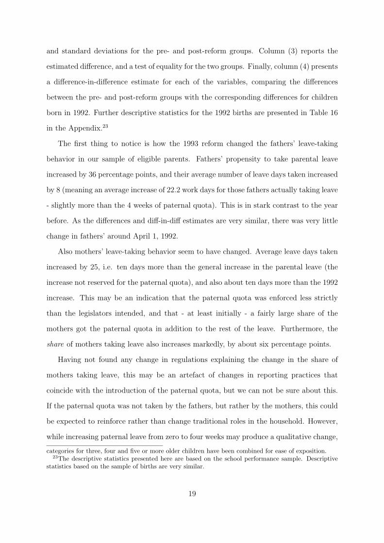
4.3 Family outcomes

Data on marriage, divorce and parity come from Statistics Norway’s family and demogra-

phy files. We investigate the impact of paternity leave on the following family outcomes:

parents’ total number of children 15 years after the reform (2008), their probability of

divorce, the probability that the father has his next child with the same woman (condi-

tional on having another child), child spacing and the number of days parent take leave

if they have another child. Table 4 provide descriptive statistics.

For the family outcomes we also construct an index. Following Deming (2009), we

20This is a natural division as compulsory schooling in Norway starts at age six.

17

Table 4: Summary statistics, family outcomes.

Mean SDMother’s parity 2.54 (0.85)Father’s parity 2.63 (0.96)Prob(Divorced by child age 14) 0.21 (0.41)Prob(Next child together) 0.87 (0.34)Child spacing (years) 3.51 (1.80)Father’s leave next child (days) 24.8 (26.4)N 17257

Note: Sample is children born during the 26 weeks surrounding April 1, 1993, excluding two weeksbefore and after April 1, divided into those born during the 13 weeks preceding the reform and thoseborn during the first 13 weeks after the reform.

decide whether an outcome is to be considered positive or negative and change the sign of

negative outcomes. Hence, completed fertility (measured as parity in 2008) for mothers

and fathers and the probability of the couple having their next child together enter

positively, whereas the probability that the couple is registered with divorce 14 years

later and the distance in time to their next child enter negatively.21

4.4 Control variables

We include control variables for parents’ age at birth of their child and level of education

and annual income the year before birth. We also control for birth order. Education is

measured (October, 1) the year before birth, and is divided into four mutually exclusive

categories; lower secondary education or less, upper secondary education, higher educa-

tion lower degree and higher education higher degree. Birth order is controlled for by

dummies for the number of children each parent already has, with six categories ranging

from zero to five or more.

Table 5 give descriptive statistics for pre-birth characteristics for eligible parents whose

children were born within a thirteen-week window prior or subsequent to April 1, 1993,

excluding two weeks before and after April 1.22 Columns (1) and (2) present averages

21Outcomes that, for obvious reasons, cannot be observed for a given family are excluded when gen-erating the index.

22The characteristics are the same as those we control for in the regression. However, in Table 5 the

18

and standard deviations for the pre- and post-reform groups. Column (3) reports the

estimated difference, and a test of equality for the two groups. Finally, column (4) presents

a difference-in-difference estimate for each of the variables, comparing the differences

between the pre- and post-reform groups with the corresponding differences for children

born in 1992. Further descriptive statistics for the 1992 births are presented in Table 16

in the Appendix.23

The first thing to notice is how the 1993 reform changed the fathers’ leave-taking

behavior in our sample of eligible parents. Fathers’ propensity to take parental leave

increased by 36 percentage points, and their average number of leave days taken increased

by 8 (meaning an average increase of 22.2 work days for those fathers actually taking leave

- slightly more than the 4 weeks of paternal quota). This is in stark contrast to the year

before. As the differences and diff-in-diff estimates are very similar, there was very little

change in fathers’ around April 1, 1992.

Also mothers’ leave-taking behavior seem to have changed. Average leave days taken

increased by 25, i.e. ten days more than the general increase in the parental leave (the

increase not reserved for the paternal quota), and also about ten days more than the 1992

increase. This may be an indication that the paternal quota was enforced less strictly

than the legislators intended, and that - at least initially - a fairly large share of the

mothers got the paternal quota in addition to the rest of the leave. Furthermore, the

share of mothers taking leave also increases markedly, by about six percentage points.

Having not found any change in regulations explaining the change in the share of

mothers taking leave, this may be an artefact of changes in reporting practices that

coincide with the introduction of the paternal quota, but we can not be sure about this.

If the paternal quota was not taken by the fathers, but rather by the mothers, this could

be expected to reinforce rather than change traditional roles in the household. However,

while increasing paternal leave from zero to four weeks may produce a qualitative change,

categories for three, four and five or more older children have been combined for ease of exposition.23The descriptive statistics presented here are based on the school performance sample. Descriptive

statistics based on the sample of births are very similar.

19

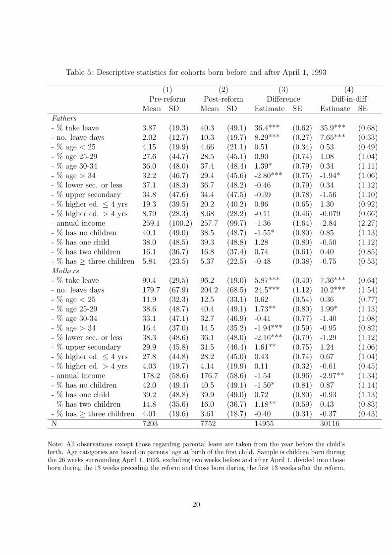
Table 5: Descriptive statistics for cohorts born before and after April 1, 1993

(1) (2) (3) (4)Pre-reform Post-reform Difference Diff-in-diff

Mean SD Mean SD Estimate SE Estimate SEFathers- % take leave 3.87 (19.3) 40.3 (49.1) 36.4*** (0.62) 35.9*** (0.68)- no. leave days 2.02 (12.7) 10.3 (19.7) 8.29*** (0.27) 7.65*** (0.33)- % age < 25 4.15 (19.9) 4.66 (21.1) 0.51 (0.34) 0.53 (0.49)- % age 25-29 27.6 (44.7) 28.5 (45.1) 0.90 (0.74) 1.08 (1.04)- % age 30-34 36.0 (48.0) 37.4 (48.4) 1.39* (0.79) 0.34 (1.11)- % age > 34 32.2 (46.7) 29.4 (45.6) -2.80*** (0.75) -1.94* (1.06)- % lower sec. or less 37.1 (48.3) 36.7 (48.2) -0.46 (0.79) 0.34 (1.12)- % upper secondary 34.8 (47.6) 34.4 (47.5) -0.39 (0.78) -1.56 (1.10)- % higher ed. ≤ 4 yrs 19.3 (39.5) 20.2 (40.2) 0.96 (0.65) 1.30 (0.92)- % higher ed. > 4 yrs 8.79 (28.3) 8.68 (28.2) -0.11 (0.46) -0.079 (0.66)- annual income 259.1 (100.2) 257.7 (99.7) -1.36 (1.64) -2.84 (2.27)- % has no children 40.1 (49.0) 38.5 (48.7) -1.55* (0.80) 0.85 (1.13)- % has one child 38.0 (48.5) 39.3 (48.8) 1.28 (0.80) -0.50 (1.12)- % has two children 16.1 (36.7) 16.8 (37.4) 0.74 (0.61) 0.40 (0.85)- % has ≥ three children 5.84 (23.5) 5.37 (22.5) -0.48 (0.38) -0.75 (0.53)Mothers- % take leave 90.4 (29.5) 96.2 (19.0) 5.87*** (0.40) 7.36*** (0.64)- no. leave days 179.7 (67.9) 204.2 (68.5) 24.5*** (1.12) 10.2*** (1.54)- % age < 25 11.9 (32.3) 12.5 (33.1) 0.62 (0.54) 0.36 (0.77)- % age 25-29 38.6 (48.7) 40.4 (49.1) 1.73** (0.80) 1.99* (1.13)- % age 30-34 33.1 (47.1) 32.7 (46.9) -0.41 (0.77) -1.40 (1.08)- % age > 34 16.4 (37.0) 14.5 (35.2) -1.94*** (0.59) -0.95 (0.82)- % lower sec. or less 38.3 (48.6) 36.1 (48.0) -2.16*** (0.79) -1.29 (1.12)- % upper secondary 29.9 (45.8) 31.5 (46.4) 1.61** (0.75) 1.24 (1.06)- % higher ed. ≤ 4 yrs 27.8 (44.8) 28.2 (45.0) 0.43 (0.74) 0.67 (1.04)- % higher ed. > 4 yrs 4.03 (19.7) 4.14 (19.9) 0.11 (0.32) -0.61 (0.45)- annual income 178.2 (58.6) 176.7 (58.6) -1.54 (0.96) -2.97** (1.34)- % has no children 42.0 (49.4) 40.5 (49.1) -1.50* (0.81) 0.87 (1.14)- % has one child 39.2 (48.8) 39.9 (49.0) 0.72 (0.80) -0.93 (1.13)- % has two children 14.8 (35.6) 16.0 (36.7) 1.18** (0.59) 0.43 (0.83)- % has ≥ three children 4.01 (19.6) 3.61 (18.7) -0.40 (0.31) -0.37 (0.43)N 7203 7752 14955 30116

Note: All observations except those regarding parental leave are taken from the year before the child’sbirth. Age categories are based on parents’ age at birth of the first child. Sample is children born duringthe 26 weeks surrounding April 1, 1993, excluding two weeks before and after April 1, divided into thoseborn during the 13 weeks preceding the reform and those born during the first 13 weeks after the reform.

20

the marginal effect of maternity leave, when it already is over 30 weeks, is likely to be

much smaller.

Other than parental leave, there are few statistically significant differences in the

pre-birth characteristics between the pre- and post-reform 1993 cohorts. Furthermore,

these are largely matched in the 1992 data, such that there is only one variable which

has a difference-in-difference significant at he 5% level, and two more at the 10% level.

With 26 variables tested, this is about what we would expect if there were no systematic

differences. Thus, on the whole Table 5 gives support to the idea of the reform providing

exogenous variation along the relevant dimension (and only this one): Parental leave.

5 Results

We now present our estimates of the causal effects of paternity leave, instrumented by

the Norwegian 1993 paternal quota reform. For brevity, we present only the LATE in

question (α in Equation 1). Tables including the coefficients on covariates are available

upon request.

Our first stage results (see Appendix Table 17) show that the excluded instrument

(Reform) is a strong predictor of paternity leave: The regression adjusted compliance

rate is 0.37 for our baseline specification.

Although the compliance rate is high and our instrument strong, 4 weeks of paternity

leave may not be considered enough time to really impact long run outcomes. In so far

as our point estimates point to zero effects, or no precise effects, this may not be taken

as proof that paternity leave does not at all have an impact on these outcomes; it may

also be that the reform is too small.

Yet, the perceived mechanism is not merely a direct link from 4 weeks spent at home

by fathers to a change in children’s school performance 15 years later, or to a penalization

by employers for the time taken off from work. Rather, in line with Becker (1985, 1991)

and the stated intentions of Norwegian policy makers, the relatively short period of

21

paternity leave is assumed to affect the evolution of household roles and labor sharing,

with a small change in initial comparative advantages yielding a larger impact on the

degree of specialization in the longer run.

For every outcome, we run four different specifications. In Tables 6 through 11, column

(1) shows the results from regressions on equation (1) on a ±13 week window (excluding

the ±2 weeks that are affected by birth timing) without controls. In column (2) we have

added the full set of family background variables available. This is our most preferred

specification. Column (3) shows results when the time window is reduced to ±7 weeks.

Lastly, in column (4) we have included the ±2 weeks affected by birth timing in the ±13

week window.

When results are discussed without explicit reference to one particular specification,

the specification in column (2) is the one in question.

5.1 Children’s school performance

There is a rapidly growing literature on the importance of early childhood development

for long term outcomes. Cunha and Heckman (2007) argue that skill formation early in

life is determinant of skill development later on. Almond and Currie (2010), who have

recently reviewed the literature in this field, state that child and family characteristics

measured at the age of five ”do as much to explain future outcomes as factors that

labor economists have more traditionally focused on, such as years of education”. Using

Norwegian data, Carneiro et al. (2010) find that maternity leave significantly increases

the probability that the child finishes high school. It is therefore of great interest to see

how children are affected by paternity leave.

For the children born at the time of the 1993 paternal quota reform, there is naturally

still a limited set of variables available. To measure cognitive skills we rely on pupils

exam scores at the end of 10th grade (in 2009). 10th grade is the last year of mandatory

schooling in Norway.

Table 6 presents the regression results for exam scores at the end of 10th grade.

22

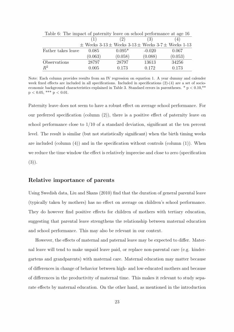
Table 6: The impact of paternity leave on school performance at age 16(1) (2) (3) (4)

± Weeks 3-13± Weeks 3-13± Weeks 3-7± Weeks 1-13Father takes leave 0.085 0.095* -0.020 0.067

(0.063) (0.058) (0.088) (0.053)Observations 28797 28797 13613 34256R2 0.005 0.173 0.172 0.173

Note: Each column provides results from an IV regression on equation 1. A year dummy and calenderweek fixed effects are included in all specifications. Included in specifications (2)-(4) are a set of socio-economic background characteristics explained in Table 3. Standard errors in parentheses. * p < 0.10,**p < 0.05, *** p < 0.01.

Paternity leave does not seem to have a robust effect on average school performance. For

our preferred specification (column (2)), there is a positive effect of paternity leave on

school performance close to 1/10 of a standard deviation, significant at the ten percent

level. The result is similar (but not statistically significant) when the birth timing weeks

are included (column (4)) and in the specification without controls (column (1)). When

we reduce the time window the effect is relatively imprecise and close to zero (specification

(3)).

Relative importance of parents

Using Swedish data, Liu and Skans (2010) find that the duration of general parental leave

(typically taken by mothers) has no effect on average on children’s school performance.

They do however find positive effects for children of mothers with tertiary education,

suggesting that parental leave strengthens the relationship between maternal education

and school performance. This may also be relevant in our context.

However, the effects of maternal and paternal leave may be expected to differ. Mater-

nal leave will tend to make unpaid leave paid, or replace non-parental care (e.g. kinder-

gartens and grandparents) with maternal care. Maternal education may matter because

of differences in change of behavior between high- and low-educated mothers and because

of differences in the productivity of maternal time. This makes it relevant to study sepa-

rate effects by maternal education. On the other hand, as mentioned in the introduction

23

Table 7: The impact of paternity leave on school performance at age 16: Interactioneffects with parental educational groups

(1) (2) (3) (4)± Weeks 3-13 ± Weeks 3-13 ± Weeks 3-7 ± Weeks 1-13

Father takes leave- father highest educ (F > M) 0.33*** 0.26** 0.17 0.21**

(0.11) (0.10) (0.16) (0.092)- equal educ (F = M) 0.015 0.030 -0.13 0.0092

(0.12) (0.11) (0.17) (0.10)- mother highest educ (F < M) -0.080 -0.0014 -0.11 -0.019

(0.098) (0.089) (0.14) (0.083)Observations 28797 28797 13613 34256R2 0.003 0.173 0.171 0.173p-value (F > M) = (F = M) 0.055 0.13 0.19 0.15p-value (F > M) = (F < M) 0.0054 0.053 0.18 0.063p-value (F = M) = (F < M) 0.55 0.83 0.91 0.83


to this section, paternity leave may impact the evolution of household roles and labor

sharing in the home. If paternity leave sets off a dynamic where the father is more in-

volved in his child and the mother becomes relatively less important, i.e. that motherly

care to some extent is replaced by fatherly care, we should expect the effect of paternity

leave to depend on parents’ relative “skill levels” as parents. More specifically, we may

expect to find a positive effect on cognitive skills when care from a highly educated father

displaces that of a less educated mother.24

Table 7 reports heterogeneous effects of paternity leave according to whether the

father has higher education than the mother, the parents have equally high education, or

the mother has higher education than the father. The results are obtained by interacting

one dummy for each possibility.25 In our sample, 35.8% of students belong to the first

24If relative education is indeed what matters, we may also expect to find some sign of a more positiveeffect for highly-educated fathers, irrespective of the mother’s education. However, this approach is likelyto severely understate the potential effect of parental leave, because of the high correlation in parents’education.

25An alternative way of addressing this question is to estimate group-specific equations, which providessimilar estimates. We prefer to interact the group indicators, as this increases precision and facilitates

24

group (F>M), 27.6% to the second (F=M), and 36.6% of students belong to the third

group (F<M). Table 18 in the Appendix shows that the first stage results are fairly

similar across the three groups - although the regression adjusted compliance rate seems

to increase with the mother being relatively higher educated.

In the families where the fathers have the highest education level we find that pater-

nity leave increases school performance with 0.26 of a standard deviation (statistically

significant at the 5% level). The effect is fairly stable across samples, but it is not statis-

tically significant at conventional levels with the ±7 weeks time window. The estimated

effect in families where mother’s education is the longest is consistently negative, but

not statistically significant. The last three rows of table 7 provide p-values from tests of

equality of the estimated coefficients. For our most preferred specification, the hypothesis

that the effect is the same for families where the father has higher education than the

mother as for families where the mother has higher education than the father, is rejected

at the 10% level. Our results are thus similar to the findings of Liu and Skans (2010), in

that the effect of parental leave differ by the parents’ education.

Daughters and sons

Tables 8 and 9 show the results from regressions run on separate samples according to the

child’s gender. We see that the effect of paternity leave on daughters’ school performance

is strong - 0.38 of a standard deviation - and statistically significant at the 5% level in

families where the father is relatively higher educated. The corresponding effect on sons’

school performance is much weaker - and not statistically significant.

There are several potential explanations for the differential gender effects. Different

uptake is not one of them: The first stage results for the subsamples show that uptake

does not differ between the groups. Fathers of sons are just as likely to take paternity

leave as fathers of daughters.26 Therefore, either paternity leave spurs a different dynamic

comparison of the group-specific coefficients.26See Tables 19 and 20 in the Appendix.

25

Table 8: The impact of paternity leave on daughters’ school performance at age 16:Interaction effects with parental educational groups


Father takes leave- father highest educ (F > M) 0.47*** 0.38** 0.26 0.33**

(0.16) (0.15) (0.22) (0.13)- equal educ (F = M) -0.033 -0.0012 -0.28 0.032

(0.17) (0.16) (0.23) (0.15)- mother highest educ (F < M) -0.048 0.012 0.040 -0.0080



Table 9: The impact of paternity leave on sons’ school performance at age 16: Interactioneffects with parental educational groups


Father takes leave- father highest educ (F > M) 0.20 0.14 0.070 0.11

(0.15) (0.14) (0.22) (0.13)- equal educ (F = M) 0.065 0.017 -0.043 -0.046

(0.17) (0.16) (0.25) (0.15)- mother highest educ (F < M) -0.12 -0.025 -0.23 -0.038



26

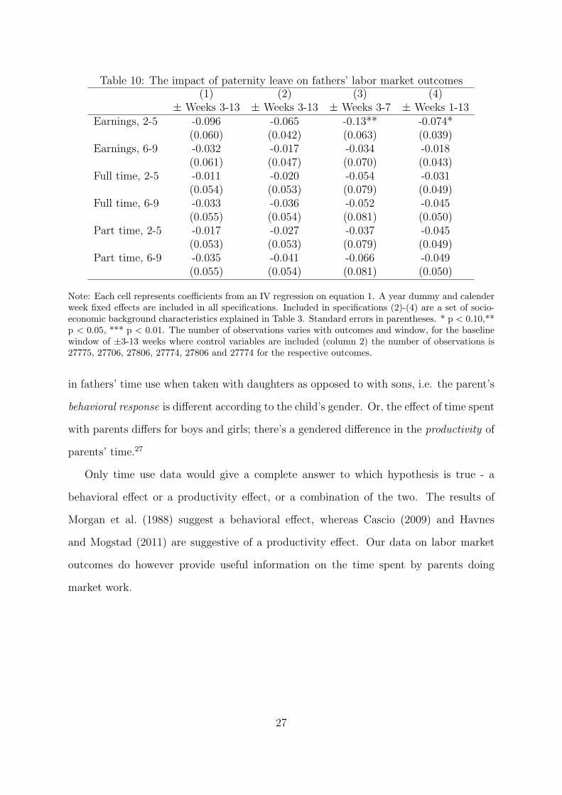
Table 10: The impact of paternity leave on fathers’ labor market outcomes(1) (2) (3) (4)

± Weeks 3-13 ± Weeks 3-13 ± Weeks 3-7 ± Weeks 1-13Earnings, 2-5 -0.096 -0.065 -0.13** -0.074*

(0.060) (0.042) (0.063) (0.039)Earnings, 6-9 -0.032 -0.017 -0.034 -0.018

(0.061) (0.047) (0.070) (0.043)Full time, 2-5 -0.011 -0.020 -0.054 -0.031

(0.054) (0.053) (0.079) (0.049)Full time, 6-9 -0.033 -0.036 -0.052 -0.045

(0.055) (0.054) (0.081) (0.050)Part time, 2-5 -0.017 -0.027 -0.037 -0.045

(0.053) (0.053) (0.079) (0.049)Part time, 6-9 -0.035 -0.041 -0.066 -0.049

(0.055) (0.054) (0.081) (0.050)

Note: Each cell represents coefficients from an IV regression on equation 1. A year dummy and calenderweek fixed effects are included in all specifications. Included in specifications (2)-(4) are a set of socio-economic background characteristics explained in Table 3. Standard errors in parentheses. * p < 0.10,**p < 0.05, *** p < 0.01. The number of observations varies with outcomes and window, for the baselinewindow of ±3-13 weeks where control variables are included (column 2) the number of observations is27775, 27706, 27806, 27774, 27806 and 27774 for the respective outcomes.

in fathers’ time use when taken with daughters as opposed to with sons, i.e. the parent’s

behavioral response is different according to the child’s gender. Or, the effect of time spent

with parents differs for boys and girls; there’s a gendered difference in the productivity of

parents’ time.27

Only time use data would give a complete answer to which hypothesis is true - a

behavioral effect or a productivity effect, or a combination of the two. The results of

Morgan et al. (1988) suggest a behavioral effect, whereas Cascio (2009) and Havnes

and Mogstad (2011) are suggestive of a productivity effect. Our data on labor market

outcomes do however provide useful information on the time spent by parents doing

market work.

27

Table 11: The impact of paternity leave on mothers’ labor market outcomes(1) (2) (3) (4)

± Weeks 3-13 ± Weeks 3-13 ± Weeks 3-7 ± Weeks 1-13Earnings, 2-5 -0.25*** -0.15*** -0.16** -0.13***

(0.061) (0.046) (0.068) (0.042)Earnings, 6-9 -0.22*** -0.14*** -0.17** -0.12***

(0.061) (0.050) (0.075) (0.046)Full time, 2-5 -0.060 -0.014 0.0014 -0.0069

(0.055) (0.050) (0.074) (0.046)Full time, 6-9 -0.077 -0.041 0.0046 -0.011

(0.055) (0.052) (0.078) (0.048)Part time, 2-5 -0.12** -0.087* -0.14* -0.079*

(0.053) (0.050) (0.075) (0.046)Part time, 6-9 -0.15*** -0.12** -0.15** -0.091*

(0.054) (0.052) (0.077) (0.047)

Note: Each cell represents coefficients from an IV regression on equation 1. A year dummy and calenderweek fixed effects are included in all specifications. Included in specifications (2)-(4) are a set of socio-economic background characteristics explained in Table 3. Standard errors in parentheses. * p < 0.10,**p < 0.05, *** p < 0.01. The number of observations varies with outcomes and window, for the baselinewindow of ±3-13 weeks where control variables are included (column 2) the number of observations is28307, 28271, 28320, 28289, 28320 and 28289 for the respective outcomes.

5.2 Labor market outcomes

Table 10 shows the results from regressions on equation (1), where the dependent variables

are the normalized averages of earnings and labor supply for fathers over the years when

the child is 2-5 years old and 6-9 years old, respectively.

Our estimated effects of paternity leave on fathers’ labor market outcomes are negative

for every outcome and across all time windows. This is consistent with the hypothesis

that paternity leave increases fathers’ involvement at home, but the estimates are (with

a few exceptions) not statistically significant. The point estimates we document are

however in line with the ones found by Rege and Solli (2010), indicating that the lack

of any statistical significant effects in our analysis may be due to low statistical power.

The identification strategy of Rege and Solli (2010) is based on the assumption that time

trends in the earnings of fathers of children of different ages through the 1990s would be

equal in the absence of the reform.

27We are thankful to Shelly Lundberg for pointing out this distinction to us.

28

Table 11 shows the corresponding results on mothers’ labor market outcomes. Con-

trary to what would be expected in a simple Beckerian framework, mothers’ earnings are

negatively affected by paternity leave, both in the short run (child age 2-5) and in the

long run (child age 6-9). In the baseline window, the effect is 0.15 of a standard deviation

reduction in earnings, statistically significant at the one percent level. Point estimates

and precision are fairly stable across time windows.

The estimated average reduction in earnings seems to be driven by a negative effect of

paternity leave on mothers’ working hours, more specifically the probability that mothers

work part time or more. Though less precise, the estimated effects on work hours are

comparable in size to the effects on earnings.

Our results on working hours, thus, provide no support for the hypothesis that pa-

ternity leave will cause households to specialize less in line with traditional gender roles:

It seems, rather, that traditional household specialization is intensified. Furthermore,

the conjecture that paternity leave causes general earning differentials between men and

women to decrease is not substantiated empirically.

The adverse effects of paternity leave on women’s labor market outcomes may be due

to complementarities in mothers’ and fathers’ time. If fathers choose to spend more time

at home and less in the market due to a family policy that strengthens the ties between

fathers and children, so do mothers.

Daughters and sons

The results on children’s school performance showed that paternity leave increased the

importance of fathers’ education for the school performance of daughters. In Table 12

we report the effects on parents’ labor market outcomes in separate samples for families

who had daughters and families who had sons. Again, the effects are much stronger in

families who had daughters. For fathers’ labor market outcomes, the point estimates are

even positive (but far from statistically significant at conventional levels) in families who

had boys. The results on mothers’ labor market outcomes reported above, are driven by

29

Table 12: The impact of paternity leave on parents’ labor market outcomes by child’sgender

(1) (2) (3) (4)Fathers of girls Fathers of boys Mothers of girls Mothers of boys

Earnings, 2-5 -0.088 -0.033 -0.26*** -0.057(0.062) (0.057) (0.066) (0.063)

Earnings, 6-9 -0.047 0.015 -0.25*** -0.032(0.069) (0.064) (0.072) (0.069)

Full time, 2-5 -0.093 0.050 -0.046 0.017(0.077) (0.073) (0.072) (0.069)

Full time, 6-9 -0.13 0.051 -0.086 -0.00077(0.078) (0.075) (0.076) (0.072)

Part time, 2-5 -0.11 0.053 -0.13* -0.046(0.077) (0.072) (0.072) (0.069)

Part time, 6-9 -0.11 0.029 -0.21*** -0.048(0.078) (0.075) (0.075) (0.071)

Note: Each cell represents coefficients from an IV regression on equation 1. A year dummy and calenderweek fixed effects are included in all specifications. Included in specifications (2)-(4) are a set of socio-economic background characteristics explained in Table 3. Standard errors in parentheses. * p < 0.10,**p < 0.05, *** p < 0.01.

the sample of families who had girls.

Our results are indicative of a gender difference in parents’ behavioral response to pa-

ternity leave, which again may contribute to the effect on daughters’ school performance

in families where fathers are relatively higher educated than mothers. As gender is unre-

lated to unobserved pre-birth characteristics, it is unlikely that the estimated differences

reflect differences in unobservables.

5.3 Family outcomes

Our analysis is completed by looking at how paternity leave affects a set of outcomes

more directly connected to family life. In light of the somewhat surprising results found

on labor market outcomes, family outcomes may be informative. For instance, if parents’

time investment in family life are complementarities, this could show up in fertility and

divorce rates.

Table 13 provides our results on family outcomes. In the baseline specification none of

30

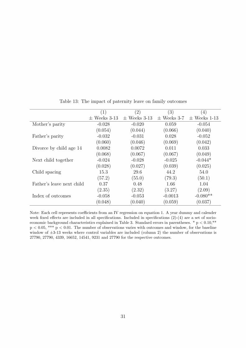
Table 13: The impact of paternity leave on family outcomes


Mother’s parity -0.028 -0.020 0.059 -0.054(0.054) (0.044) (0.066) (0.040)

Father’s parity -0.032 -0.031 0.028 -0.052(0.060) (0.046) (0.069) (0.042)

Divorce by child age 14 0.0082 0.0072 0.011 0.033(0.068) (0.067) (0.067) (0.049)

Next child together -0.024 -0.028 -0.025 -0.044*(0.028) (0.027) (0.039) (0.025)

Child spacing 15.3 29.6 44.2 54.0(57.2) (55.0) (79.3) (50.1)

Father’s leave next child 0.37 0.48 1.66 1.04(2.35) (2.32) (3.27) (2.09)

Index of outcomes -0.058 -0.053 -0.0013 -0.080**(0.048) (0.040) (0.059) (0.037)

Note: Each cell represents coefficients from an IV regression on equation 1. A year dummy and calenderweek fixed effects are included in all specifications. Included in specifications (2)-(4) are a set of socio-economic background characteristics explained in Table 3. Standard errors in parentheses. * p < 0.10,**p < 0.05, *** p < 0.01. The number of observations varies with outcomes and window, for the baselinewindow of ±3-13 weeks where control variables are included (column 2) the number of observations is27790, 27790, 4339, 16652, 14541, 9231 and 27790 for the respective outcomes.

31

these are statistically significant. The lack of effects on family outcomes affects the scope

for potential mechanisms through which paternity leave influences other outcomes. For

example, the negative effects on mothers’ earnings and employment could have followed

from an increase in subsequent fertility. Our results indicate that this is not the case.

As referred in Lundberg and Rose (2004), several authors have reported that, in the

United States, having a son relative to a daughter increases the likelihood that a marriage

will remain intact. In light of this, it may be that our finding no average effects may

conceal heterogeneous effects according to gender. Indeed, it turns out that the point

estimates consistently have opposite signs in the two samples, although the differences

are mostly statistically insignificant.28

5.4 Characterizing compliers

Since any instrumental variable strategy identifies effects only for the subpopulation af-

fected by the instrument, external validity is always a concern (Moffitt (2005)). It is

therefore useful to characterize families whose behavior was actually affected by the pa-

ternal quota reform - ‘compliers’ in the terminology of Imbens and Angrist (1994). If the

compliant subpopulation is similar to the general population, the case for extrapolating

estimated causal effects to the general population is stronger.

Table 14 presents the likelihood that a complier has a particular characteristic relative

to the population of eligible families. This is obtained by taking the ratio of the first stage

across a particular covariate group to the overall first-stage (Angrist and Pischke (2009),

Angrist and Fernandez-Val (2010)).29

Fathers in the compliant subpopulation have somewhat higher education and age than

the average for fathers in our sample of eligible families. When it comes to income and

work experience, there are slightly fewer compliant fathers in both the lowest and highest

28The results can be seen in Table 21 in the Appendix.29We report results for all covariates we use in our regression analysis. While ’annual income’ and

’years of employment’ enters linearly in our regression analysis, we have split them in quartiles for thepurpose of characterizing the complier group.

32

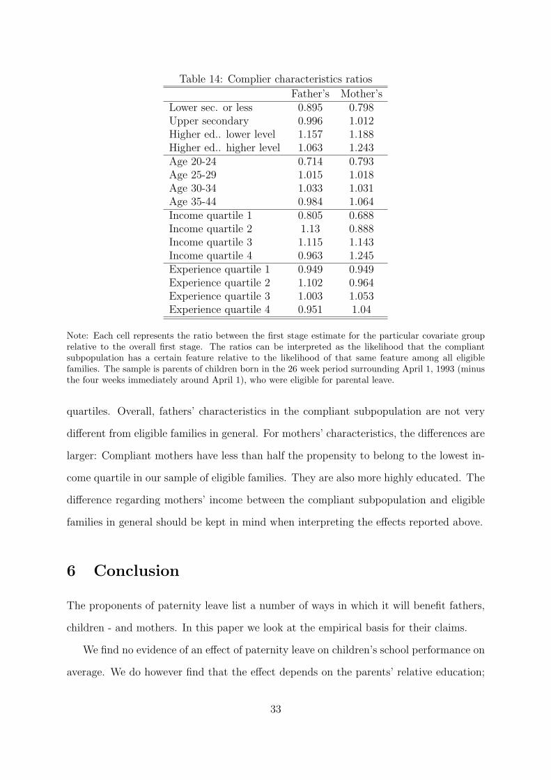
Table 14: Complier characteristics ratios

Father’s Mother’sLower sec. or less 0.895 0.798Upper secondary 0.996 1.012Higher ed.. lower level 1.157 1.188Higher ed.. higher level 1.063 1.243Age 20-24 0.714 0.793Age 25-29 1.015 1.018Age 30-34 1.033 1.031Age 35-44 0.984 1.064Income quartile 1 0.805 0.688Income quartile 2 1.13 0.888Income quartile 3 1.115 1.143Income quartile 4 0.963 1.245Experience quartile 1 0.949 0.949Experience quartile 2 1.102 0.964Experience quartile 3 1.003 1.053Experience quartile 4 0.951 1.04

Note: Each cell represents the ratio between the first stage estimate for the particular covariate grouprelative to the overall first stage. The ratios can be interpreted as the likelihood that the compliantsubpopulation has a certain feature relative to the likelihood of that same feature among all eligiblefamilies. The sample is parents of children born in the 26 week period surrounding April 1, 1993 (minusthe four weeks immediately around April 1), who were eligible for parental leave.

quartiles. Overall, fathers’ characteristics in the compliant subpopulation are not very

different from eligible families in general. For mothers’ characteristics, the differences are

larger: Compliant mothers have less than half the propensity to belong to the lowest in-

come quartile in our sample of eligible families. They are also more highly educated. The

difference regarding mothers’ income between the compliant subpopulation and eligible

families in general should be kept in mind when interpreting the effects reported above.

6 Conclusion

The proponents of paternity leave list a number of ways in which it will benefit fathers,

children - and mothers. In this paper we look at the empirical basis for their claims.

We find no evidence of an effect of paternity leave on children’s school performance on

average. We do however find that the effect depends on the parents’ relative education;

33

where children of fathers with higher education than the mother benefit from paternity

leave. This is an indication that paternity leave causes a shift from motherly to fatherly

care at home.

This shift is not mirrored in the parents’ labor market outcomes, however. That

mothers seem to respond to paternity leave by reducing labor supply is at odds with

the standard economic framework emphasizing specialization in household vs. market

work. Our analysis suggests that family-oriented policies, even if directed towards fathers,

may be ill suited to reducing earnings differentials between men and women. Further

investigation into the mechanisms behind the negative effects on mothers’ earnings and

labor supply is needed. One possible explanation is that mothers’ and fathers’ time at

home are complements.

This paper also shows that family policies may work differently according to the child’s

gender, because parents respond differently to the policy depending on whether they have

a son or a daughter. We have shown that the difference is not in terms of compliance

with the policy, but rather that it lies in how the policy makes parents behave. This

finding needs to be further investigated.

References

Almond, D. and Currie, J. (2010). Human capital development before age five. In

Ashenfelter, O. and Card, D. E., editors, Handbook of Labor Economics, volume 4.

North Holland.

Andersson, G., Hank, K., Rønsen, M., and Vikat, A. (2006). Gendering family compo-

sition: Sex preferences for children and childbearing behavior in the nordic countries.

Demography, 43(2):255 – 267.

Angrist, J. and Fernandez-Val, I. (2010). Extrapolate-ing: External validity and overi-

dentification in the late framework. NBER working paper 16566.

34

Angrist, J. D. and Pischke, J.-S. (2009). Mostly Harmless Econometrics: An Empiricist’s

Companion. Princeton University Press, NJ: Princeton.

Baker, M. and Milligan, K. S. (2011). Maternity leave and children’s cognitive and

behavioral development.

Becker, G. (1991). A Treatise on the Family. Harvard University Press, MA: Cambridge.

Becker, G. S. (1985). Human capital, effort, and the sexual division of labor. Journal of

Labor Economics, 3(1):pp. S33–S58.

Brandth, B. and Øverli, B. (1998). Omsorgspermisjon med ”kjærlig tvang”: en kartleg-

ging av fedrekvoten. Rapport. Trondheim: Allforsk.

Bratsberg, B. and Raaum, O. (2010). Immigration and wages: Evidence from construc-

tion. CReAM Discussion Paper Series no. 06/10.

Brenn, T. and Ytterstad, E. (1997). Daglige fødselstall for norge 1989-93. Tidsskrift for

den norske legeforening, 117:1098–101.

Buckles, K. and Hungerman, D. M. (2008). Season of birth and later outcomes: Old

questions, new answers. NBER working paper 14573.

Carneiro, P., Løken, K., and Salvanes, K. G. (2010). A flying start? long term conse-

quences of time investments in infants in their first year of life. Memo University of

Bergen.

Cascio, E. U. (2009). Do investments in universal early education pay off? long-term

effects of introducing kindergartens into public schools. NBER working paper 14951.

Cunha, F. and Heckman, J. (2007). The technology of skill formation. American Eco-

nomic Review, 97(2):31–47.

Deming, D. (2009). Early childhood intervention and life-cycle skill development: Evi-

dence from head start. American Economic Journal: Applied Economics, 1(3):111–34.

35

Ekberg, J., Eriksson, R., and Friebel, G. (2005). Parental leave - a policy evaluation of

the swedish ’daddy month’ reform. IZA Discussion Paper No. 1617.

Gans, J. S. and Leigh, A. (2009). Born on the first of july: An (un)natural experiment

in birth timing. Journal of Public Economics, 93(1-2):246 – 263.

Havnes, T. and Mogstad, M. (2011). No child left behind: Subsidized child care and

children’s long-run outcomes. American Economic Journal: Economic Policy, 3(2):97–

129.

Imbens, G. W. and Angrist, J. D. (1994). Identification and estimation of local average

treatment effects. Econometrica, 62(2):467–475.

Johansson, E.-A. (2010). The effect of own and spousal parental leave on earnings. IFAU

working paper 2010:4.

Kling, J. R., Liebman, J. B., and Katz, L. F. (2007). Experimental analysis of neighbor-

hood effects. Econometrica, 75(1):83–119.

Lalive, R. and Zweimuller, J. (2009). How does parental leave affect fertility and return

to work? evidence from two natural experiments. Quarterly Journal of Economics,

124(3):1363–1402.

Liu, Q. and Skans, O. N. (2010). The duration of paid parental leave and children’s

scholastic performance. The B.E. Journal of Economic Analysis and Policy, 10(1).

Lundberg, S. (2005). Sons, daughters, and parental behaviour. Oxford Review of Eco-

nomic Policy, 21(3):340–356.

Lundberg, S. and Rose, E. (2004). Investments in sons and daughters: Evidence from the

consumer expenditure survey. In Kalil, A. and DeLeire, T., editors, Family Investments

in Children: Resources and Behaviors that Promote Success, pages 163–180. Erlbaum.

Moffitt, R. (2005). Remarks on the analysis of causal relationships in population research.

Demography, 42(1):pp. 91–108.

36

Morgan, S. P., Lye, D. N., and Condran, G. A. (1988). Sons, daughters, and the risk of

marital disruption. The American Journal of Sociology, 94(1):pp. 110–129.

Rege, M. and Solli, I. (2010). The impact of paternity leave on long-term father involve-

ment. CESifo Working Paper No. 3130.

Strøm, B. (2004). Student achievement and birthday effects. Memo Norwegian University

of Science and Technology.

37

7 Appendix

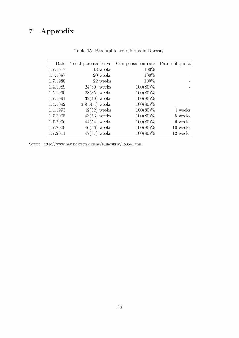
Table 15: Parental leave reforms in Norway

Date Total parental leave Compensation rate Paternal quota1.7.1977 18 weeks 100% -1.5.1987 20 weeks 100% -1.7.1988 22 weeks 100% -1.4.1989 24(30) weeks 100(80)% -1.5.1990 28(35) weeks 100(80)% -1.7.1991 32(40) weeks 100(80)% -1.4.1992 35(44.4) weeks 100(80)% -1.4.1993 42(52) weeks 100(80)% 4 weeks1.7.2005 43(53) weeks 100(80)% 5 weeks1.7.2006 44(54) weeks 100(80)% 6 weeks1.7.2009 46(56) weeks 100(80)% 10 weeks1.7.2011 47(57) weeks 100(80)% 12 weeks

Source: http://www.nav.no/rettskildene/Rundskriv/183541.cms.

38

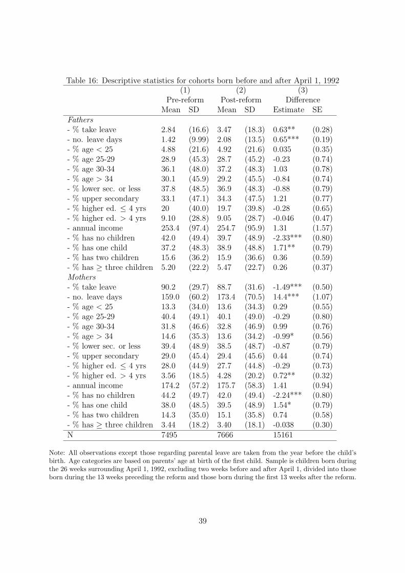
Table 16: Descriptive statistics for cohorts born before and after April 1, 1992(1) (2) (3)

Pre-reform Post-reform DifferenceMean SD Mean SD Estimate SE

Fathers- % take leave 2.84 (16.6) 3.47 (18.3) 0.63** (0.28)- no. leave days 1.42 (9.99) 2.08 (13.5) 0.65*** (0.19)- % age < 25 4.88 (21.6) 4.92 (21.6) 0.035 (0.35)- % age 25-29 28.9 (45.3) 28.7 (45.2) -0.23 (0.74)- % age 30-34 36.1 (48.0) 37.2 (48.3) 1.03 (0.78)- % age > 34 30.1 (45.9) 29.2 (45.5) -0.84 (0.74)- % lower sec. or less 37.8 (48.5) 36.9 (48.3) -0.88 (0.79)- % upper secondary 33.1 (47.1) 34.3 (47.5) 1.21 (0.77)- % higher ed. ≤ 4 yrs 20 (40.0) 19.7 (39.8) -0.28 (0.65)- % higher ed. > 4 yrs 9.10 (28.8) 9.05 (28.7) -0.046 (0.47)- annual income 253.4 (97.4) 254.7 (95.9) 1.31 (1.57)- % has no children 42.0 (49.4) 39.7 (48.9) -2.33*** (0.80)- % has one child 37.2 (48.3) 38.9 (48.8) 1.71** (0.79)- % has two children 15.6 (36.2) 15.9 (36.6) 0.36 (0.59)- % has ≥ three children 5.20 (22.2) 5.47 (22.7) 0.26 (0.37)Mothers- % take leave 90.2 (29.7) 88.7 (31.6) -1.49*** (0.50)- no. leave days 159.0 (60.2) 173.4 (70.5) 14.4*** (1.07)- % age < 25 13.3 (34.0) 13.6 (34.3) 0.29 (0.55)- % age 25-29 40.4 (49.1) 40.1 (49.0) -0.29 (0.80)- % age 30-34 31.8 (46.6) 32.8 (46.9) 0.99 (0.76)- % age > 34 14.6 (35.3) 13.6 (34.2) -0.99* (0.56)- % lower sec. or less 39.4 (48.9) 38.5 (48.7) -0.87 (0.79)- % upper secondary 29.0 (45.4) 29.4 (45.6) 0.44 (0.74)- % higher ed. ≤ 4 yrs 28.0 (44.9) 27.7 (44.8) -0.29 (0.73)- % higher ed. > 4 yrs 3.56 (18.5) 4.28 (20.2) 0.72** (0.32)- annual income 174.2 (57.2) 175.7 (58.3) 1.41 (0.94)- % has no children 44.2 (49.7) 42.0 (49.4) -2.24*** (0.80)- % has one child 38.0 (48.5) 39.5 (48.9) 1.54* (0.79)- % has two children 14.3 (35.0) 15.1 (35.8) 0.74 (0.58)- % has ≥ three children 3.44 (18.2) 3.40 (18.1) -0.038 (0.30)N 7495 7666 15161

Note: All observations except those regarding parental leave are taken from the year before the child’sbirth. Age categories are based on parents’ age at birth of the first child. Sample is children born duringthe 26 weeks surrounding April 1, 1992, excluding two weeks before and after April 1, divided into thoseborn during the 13 weeks preceding the reform and those born during the first 13 weeks after the reform.

39

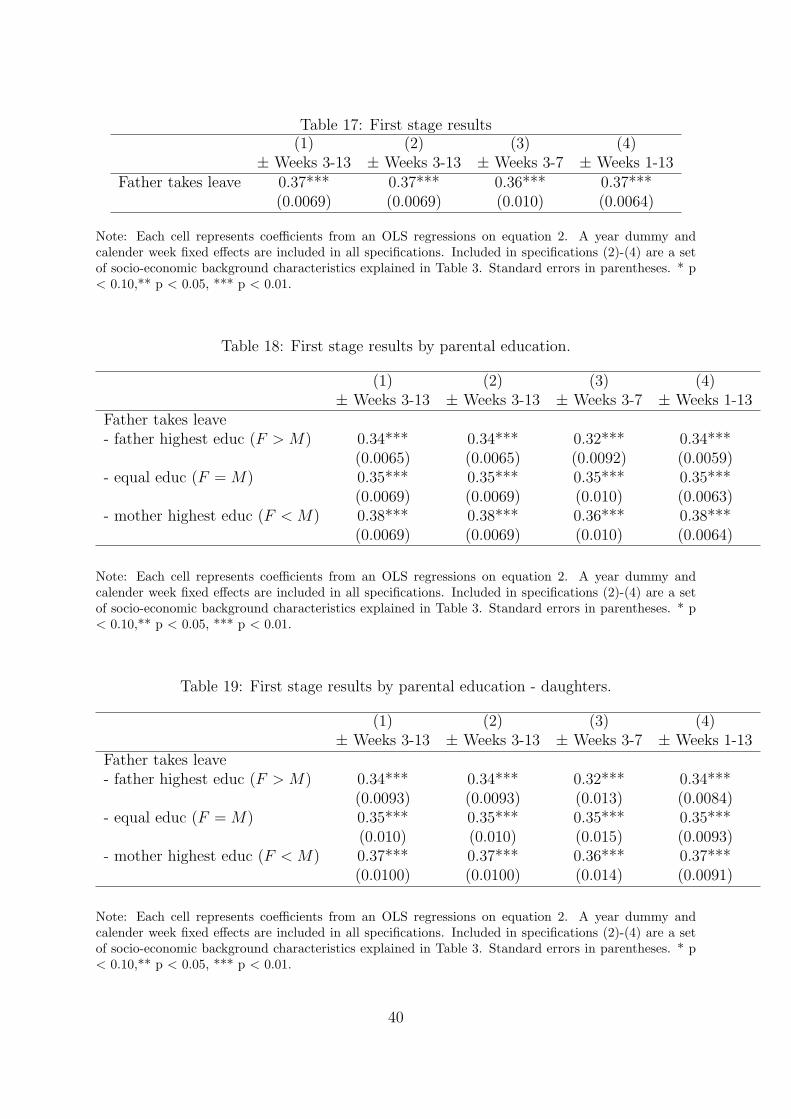
Table 17: First stage results(1) (2) (3) (4)

± Weeks 3-13 ± Weeks 3-13 ± Weeks 3-7 ± Weeks 1-13Father takes leave 0.37*** 0.37*** 0.36*** 0.37***

(0.0069) (0.0069) (0.010) (0.0064)

Note: Each cell represents coefficients from an OLS regressions on equation 2. A year dummy andcalender week fixed effects are included in all specifications. Included in specifications (2)-(4) are a setof socio-economic background characteristics explained in Table 3. Standard errors in parentheses. * p< 0.10,** p < 0.05, *** p < 0.01.

Table 18: First stage results by parental education.


Father takes leave- father highest educ (F > M) 0.34*** 0.34*** 0.32*** 0.34***

(0.0065) (0.0065) (0.0092) (0.0059)- equal educ (F = M) 0.35*** 0.35*** 0.35*** 0.35***

(0.0069) (0.0069) (0.010) (0.0063)- mother highest educ (F < M) 0.38*** 0.38*** 0.36*** 0.38***

(0.0069) (0.0069) (0.010) (0.0064)


Table 19: First stage results by parental education - daughters.



(0.0093) (0.0093) (0.013) (0.0084)- equal educ (F = M) 0.35*** 0.35*** 0.35*** 0.35***


(0.0100) (0.0100) (0.014) (0.0091)


40

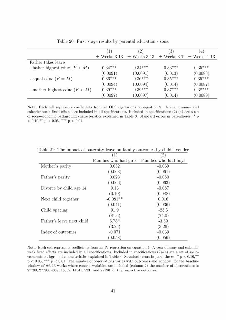
Table 20: First stage results by parental education - sons.



(0.0091) (0.0091) (0.013) (0.0083)- equal educ (F = M) 0.36*** 0.36*** 0.35*** 0.35***


(0.0097) (0.0097) (0.014) (0.0089)


Table 21: The impact of paternity leave on family outcomes by child’s gender(1) (2)

Families who had girls Families who had boysMother’s parity 0.032 -0.069

(0.063) (0.061)Father’s parity 0.023 -0.080

(0.066) (0.063)Divorce by child age 14 0.13 -0.087

(0.10) (0.088)Next child together -0.081** 0.016

(0.041) (0.036)Child spacing 91.9 -23.5

(81.6) (74.0)Father’s leave next child 5.78* -3.59

(3.25) (3.26)Index of outcomes -0.071 -0.039

(0.058) (0.056)

Note: Each cell represents coefficients from an IV regression on equation 1. A year dummy and calenderweek fixed effects are included in all specifications. Included in specifications (2)-(4) are a set of socio-economic background characteristics explained in Table 3. Standard errors in parentheses. * p < 0.10,**p < 0.05, *** p < 0.01. The number of observations varies with outcomes and window, for the baselinewindow of ±3-13 weeks where control variables are included (column 2) the number of observations is27790, 27790, 4339, 16652, 14541, 9231 and 27790 for the respective outcomes.

41

sara cools, jon h. fiva and lars johannessen kirkebøen · sara cools, jon h. fiva and lars...

Documents